Diagrammatic auxiliary particle Diagrammatic auxiliary particle impurity solvers - SUNCAimpurity solvers - SUNCA

• Auxiliary particle method• How to set up perturbation theory?• How to choose diagrams?• Where Luttinger Ward functional comes in?• How to write down end evaluate Bethe-

Salpeter equation?• How to solve SUNCA integral equations?• Some results and comparison• Summary

Advantages/DisadvantagesAdvantages/Disadvantages

Advantages:Advantages:•Fast (compared to QMC) IS with no additional time cost for large NFast (compared to QMC) IS with no additional time cost for large N•Defined and numerically solved on real axis (more information)Defined and numerically solved on real axis (more information)

Disadvantages:Disadvantages:•Not exact and needs to be carefully tested and benchmarked Not exact and needs to be carefully tested and benchmarked (breaks down at low temperature T<<Tk – but gets (breaks down at low temperature T<<Tk – but gets

better with increasing N)better with increasing N)•No straightforward extension to a non-degenerate AIM No straightforward extension to a non-degenerate AIM (relays on(relays on

degeneracy of local states)degeneracy of local states) – but straightforward extension to – but straightforward extension to out-of-equilibrium AIMout-of-equilibrium AIM

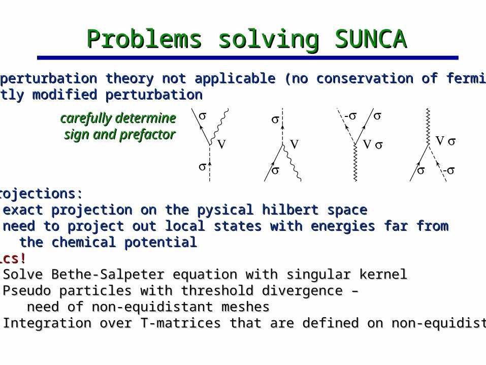
Problems solving SUNCAProblems solving SUNCA

•Usual perturbation theory not applicable (no conservation of fermions)Usual perturbation theory not applicable (no conservation of fermions) slightly modified perturbationslightly modified perturbation

carefully determine carefully determine sign and prefactorsign and prefactor

•Two projections:Two projections:•exact projection on the pysical hilbert spaceexact projection on the pysical hilbert space•need to project out local states with energies far from need to project out local states with energies far from

the chemical potentialthe chemical potential•Numerics!Numerics!

•Solve Bethe-Salpeter equation with singular kernelSolve Bethe-Salpeter equation with singular kernel•Pseudo particles with threshold divergence –Pseudo particles with threshold divergence –

need of non-equidistant meshesneed of non-equidistant meshes•Integration over T-matrices that are defined on non-equidistant meshIntegration over T-matrices that are defined on non-equidistant mesh

Diagrammatic auxiliary particle Diagrammatic auxiliary particle impurity solversimpurity solvers

• Exact diagonalization of the interacting region (impurity site or cluster)

• Introduction of auxiliary particles

# electrons in even is boson # electrons in odd is fermion

• Local constraint (completeness relation) for pseudo particles:

Local constraint and HamiltonianLocal constraint and Hamiltonian

Hamiltonian in auxiliary representationHamiltonian in auxiliary representation

Representation of local operators

local hamiltonian quadratic (solved exactly)local hamiltonian quadratic (solved exactly)

bath hamiltonian is quadraticbath hamiltonian is quadratic

perturbation theory in coupling between both possibleperturbation theory in coupling between both possible

RemarksRemarks

•Why do we introduce “unnecessary” new degrees of freedom? Why do we introduce “unnecessary” new degrees of freedom? (auxiliary particles)(auxiliary particles)

Interaction is transferred from term U to term VInteraction is transferred from term U to term VCoulomb repulsion U is usually large and V is smallCoulomb repulsion U is usually large and V is smallBut the perturbation in V is singular!But the perturbation in V is singular!

Unlike the Hubbard operator, the auxiliary particles are Unlike the Hubbard operator, the auxiliary particles are fermions and bosons and the Wick’s theorem is validfermions and bosons and the Wick’s theorem is validPerturbation expansion is possiblePerturbation expansion is possible

Example: 1band AIMExample: 1band AIM

Diagrammatic solutionsDiagrammatic solutions

•Since the perturbation expansion in V is singular it is desirable toSince the perturbation expansion in V is singular it is desirable to sum infinite infinite number of diagrams (certain subclass). This is sum infinite infinite number of diagrams (certain subclass). This is necessary to get correct low energy manybody scale Tnecessary to get correct low energy manybody scale TK K . . •Definition of the approximation is done by defining the Luttinger-Ward Definition of the approximation is done by defining the Luttinger-Ward functional :functional :

Fully dressed pseudoparticle Green’s functionsFully dressed pseudoparticle Green’s functions

•Procedure guarantees that the approximation is conservingProcedure guarantees that the approximation is conservingfor example:for example:

Infinite U AIM within NCAInfinite U AIM within NCA

Gives correct energy scale Gives correct energy scale Works for T>0.2 TWorks for T>0.2 TKK

Below this temperature Abrikosov-Suhl resonance Below this temperature Abrikosov-Suhl resonance exceeds unitarity limitexceeds unitarity limitGives exact non-Fermi liquid exponents in the case Gives exact non-Fermi liquid exponents in the case

of 2CKMof 2CKM

Naive extension to finite U very badly failsNaive extension to finite U very badly failsTTKK several orders of magnitude too small several orders of magnitude too small

How to extend to finite U?How to extend to finite U?

Schrieffer-Wolff transformationSchrieffer-Wolff transformation

Luttinger-Ward functional for SUNCALuttinger-Ward functional for SUNCA

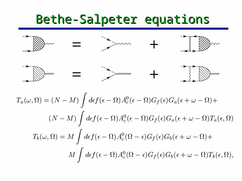
Bethe-Salpeter equationsBethe-Salpeter equations

Pseudo-fermion self-energyPseudo-fermion self-energy

Light pseudo-boson self-energyLight pseudo-boson self-energy

Heavy pseudo-boson self-energyHeavy pseudo-boson self-energy

Physical spectral function (bath self-Physical spectral function (bath self-energy)energy)

Physical spectral functionPhysical spectral function

Scaling of TScaling of TKK

Comparison with NRGComparison with NRG

Comparison with QMC and IPTComparison with QMC and IPT

Comparison with QMC T=0.5Comparison with QMC T=0.5

Comparison with QMC T=0.0625Comparison with QMC T=0.0625

Comparison with QMC T=0.0625Comparison with QMC T=0.0625

T-dependence for t2g DOST-dependence for t2g DOS

Doping dep. for t2g DOSDoping dep. for t2g DOS

SummarySummary

• To get correct energy scale for infinite U AIM, self-consistent method is needed

• Infinite series of skeleton diagrams is needed to recover correct low energy scale of the AIM at finite Coulomb interaction U

• The method can be extended to multiband case (with no additional effort)

• Diagrammatic method can be used to solve the cluster DMFT equations.

Exact projection onto Q=1 subspaceExact projection onto Q=1 subspace•Hamiltonian commutes with Q Q constant in timeHamiltonian commutes with Q Q constant in time•Q takes only integer values (Q=0,1,2,3,...)Q takes only integer values (Q=0,1,2,3,...)•How to project out only Q=1?How to project out only Q=1?

Add Lagrange multiplierAdd Lagrange multiplier

IfIf thenthen

Proof:Proof:

Exact projection in practiceExact projection in practice

How can we impose limit analytically?How can we impose limit analytically?

Only integral around branch-cut of bath Green’s function survives Only integral around branch-cut of bath Green’s function survives (bath=Green’s functions of quantities with nonzero expectation value in Q=0 subspace)(bath=Green’s functions of quantities with nonzero expectation value in Q=0 subspace)

Exact projection is done analytically!Exact projection is done analytically!

Physical quantitiesPhysical quantities

Exact relation:Exact relation:

Dyson equation:Dyson equation:

In grand-canonical ensembleIn grand-canonical ensemble