Embed Size (px)
Citation preview

DEVELOPMENT OF PHASE RETRIEVAL
TECHNIQUES IN OPTICAL MEASUREMENT
BY
NIU HONGTAO
(M. Eng.)
A THESIS SUBMITTED
FOR THE DEGREE OF DOCTOR OF PHILOSOPHY
DEPARTMENT OF MECHANICAL ENGINEERING
NATIONAL UNIVERSITY OF SINGAPORE
2011

ACKNOWLEDGEMENTS
i
ACKNOWLEDGEMENTS
The author would like to take this opportunity to gratefully acknowledge his
supervisors A/Prof. Quan Chenggen and A/Prof. Tay Cho Jui for their favorable
suggestions and technical discussions throughout the research. It is their inspiration,
guidance and support that enable him to complete this work.
The author would like to acknowledge all staffs of the Experimental Mechanics
Laboratory and the Strength of Materials Lab for their helps with experimental setup
and general advice during his study. The author would like to thank Dr. Basanta
Bhaduri for his invaluable suggestions.
The author would also like to thank his peer research students for their favorable
discussions and helps in the Laboratory.
Finally, the author is forever indebted to his parents for their understanding, endless
patience and encouragement when it was most required.

TABLE OF CONTENTS
ii
TABLE OF CONTENTS
ACKNOWLEDGEMENTS i
TABLE OF CONTENTS ii
SUMMARY v
LIST OF TABLES vii
LIST OF FIGURES viii
NOMENCLATURE xii
CHAPTER 1 INTRODUCTION 1
1.1 Optical measurement techniques 1
1.2 Challenges in optical measurement 4
1.2.1 Phase retrieval 5
1.2.2 Phase unwrapping 6
1.3 Work scope 7
1.4 Outline of thesis 8
CHAPTER 2 LITERATURE REVIEW 10
2.1 Review of optical techniques for measurement 10
2.1.1 Incoherent optical measurement techniques 10
2.1.1.1 Shadow moiré interferometry 10
2.1.1.2 Fringe projection technique 13
2.1.2 Coherent optical measurement techniques 14
2.1.2.1 Electronic speckle pattern interferometry (ESPI) 14
2.1.2.2 Digital speckle shearing interferometry (DSSI) 19
2.1.2.3 Multiple-wavelength interferometry 22
2.1.3 Phase retrieval techniques 25

TABLE OF CONTENTS
iii
2.1.3.1 Phase shifting techniques 25
2.1.3.2 Fourier transform method 26
2.2 Continuous wavelet transform (CWT) in optical measurement 31
2.3 Windowed Fourier transform (WFT) in optical measurement 39
CHAPTER 3 DEVELOPMENT OF THEORY 45
3.1 Two-dimensional (2D) CWT for phase retrieval 45
3.1.1 Limitations of previous 2D CWT 47
3.1.2 Advanced 2D Gabor CWT 50
3.2 Improved WFT for fringe demodulation 55
3.2.1 Limitations of WFT with convolution algorithm 55
3.2.2 Phase retrieval using improved WFT 56
3.2.3 Suppression of boundary effect 60
3.3 Phase fringe denoising using windowed Fourier filtering 62
3.3.1 Phase retrieval for relatively large deformation measurement 63
3.3.1.1 Windowed Fourier filtering 63
3.3.1.2 Iterative sine-cosine average filtering 65
3.3.2 Combined filtering technique for noise reduction 66
3.3.2.1 Phase error correction algorithm 68
CHAPTER 4 EXPERIMENTAL WORK 72
4.1 ESPI with carriers 72
4.2 DSSI with carriers 74
4.3 ESPI with temporal phase shifting 75
4.4 Two-wavelength DSSI system 77
CHAPTER 5 RESULTS AND DISCUSSION 80
5.1 Two-dimensional CWT for phase retrieval in ESPI 80
5.1.1 Simulation results 80

TABLE OF CONTENTS
iv
5.1.2 Experimental results 85
5.2 Improved WFT for fringe demodulation in DSSI 89
5.2.1 Simulated analysis 89
5.2.2 Experimental results 96
5.3 Relatively large deformation measurement 100
5.3.1 Phase fringe denoising in ESPI 100
5.3.1.1 Simulated results 100
5.3.1.2 Experimental results 103
5.3.2 Phase fringe denoising in DSSI 106
5.4 Two-wavelength DSSI using combined filter 111
CHAPTER 6 CONCLUSIONS AND RECOMMENDATIONS 117
6.1 Concluding remarks 117
6.2 Recommendations 119
REFERENCES 121
APPENDICES 131
Appendix A. Code for 2D Gabor and 2D fan CWT 131
Appendix B. Code for improved WFT 136
Appendix C. List of publications 141

SUMMARY
v
SUMMARY
Optical measurement techniques are very important in industry for their widely
varying applications such as nondestructive testing and phase retrieval. In this thesis,
time-frequency analysis based algorithms for optical phase retrieval in digital speckle
interference measurement were studied. To improve the noise reduction capability of
the phase retrieval techniques, two-dimensional (2D) Gabor continuous wavelet
transform (CWT) and advanced windowed Fourier transform (WFT) were developed
for phase retrieval and noise reduction for noisy fringe patterns.
A new algorithm of 2D Gabor CWT for speckle noise reduction and phase
retrieval was developed for speckle fringe pattern demodulation with carriers.
Experiment using electronic speckle pattern interferometry (ESPI) was conducted to
measure the deformation on an object surface with sub-wavelength sensitivity.
Compared with other time-frequency analysis based algorithms, such as Fourier
transform, one-dimensional (1D) CWT and 2D fan CWT, the proposed 2D Gabor
CWT has better noise immunity for speckle fringe demodulation. In addition, the
proposed 2D Gabor CWT overcomes the problem of previous 2D fan CWT which
fails to reduce speckle noise or show correct phase values in some speckle fringe
patterns due to the narrow bandwidth of 2D fan wavelet. The experimental results
obtained have validated the proposed algorithm.

SUMMARY
vi
Another new algorithm of improved WFT for phase retrieval from speckle
fringe patterns was also proposed in this thesis. Windowed Fourier transform is an
important time-frequency analysis algorithm based on Fourier transform in fringe
analysis. Unlike CWT which has a variable resolution, WFT has a fixed time and
frequency resolution in the processing of fringe patterns. The appropriate window size
in both space and frequency domain is favorable in noise reduction and phase
retrieval. Windowed Fourier transform has promising potential in fringe analysis and
the highly efficient algorithm of WFT can reduce computation time. The proposed
advanced WFT which employs fast Fourier transform reduces the computation time
significantly compared with the previous WFT with convolution method. The
experimental results obtained on out-of-plane displacement derivative measurement
using digital speckle-shearing interferometry (DSSI) have also shown a good noise
reduction capability of the proposed method. It is observed that the proposed CWT
and WFT have a good noise reduction capability in phase retrieval and subsequently
better phase fringe patterns can be obtained.
A two-wavelength DSSI using simultaneous red and green lights illumination
was also proposed. Windowed Fourier transform was employed for phase retrieval of
the speckle phase fringe patterns obtained by phase shifting method and it shows
better results than the sine-cosine average filtering method. Furthermore, a phase error
correction algorithm was also proposed to improve the sensitivity of the proposed
technique.
A list of publications arising from this research is shown in Appendix C.

LIST OF TABLES
vii
LIST OF TABLES
Table 5.1 Comparison between the proposed method and the WFF with convolution method
94
Table 5.2 Comparison of RMSE between the Fourier transform, 2D Gabor CWT and proposed WFF method
95
Table 5.3 Parameters used for the fast WFF algorithm 113

LIST OF FIGURES
viii
LIST OF FIGURES
Fig. 2.1 Shadow moiré fringe pattern on a coin’s surface
11
Fig. 2.2 Schematic diagram of shadow moiré technique
12
Fig. 2.3 Phase shifting ESPI setup
18
Fig. 2.4 A schematic drawing of DSSI
22
Fig. 2.5 (a) A simulated intensity signal with a normally distributed random noise; (b) Fourier spectrum of the signal; (c) selected positive first order spectrum from (b); (d) retrieved wrapped phase; (e) unwrapped phase
30
Fig. 2.6 (a) A 1D Morlet wavelet and its spectrum; (b) a scalogram of ( , )Wf q m for the signal shown in Fig. 2.5(a) and the dash line
represents the ridge of CWT; (c) unwrapped phase using CWT
38
Fig. 2.7 Basis of transform for time-frequency analysis
39
Fig. 3.1 (a) Real part of a 2D Morlet wavelet; (b) imaginary part of a 2D Morlet wavelet; (c) Fourier spectrum of a 2D Morlet wavelet
47
Fig. 3.2 (a) Real part of a 2D fan wavelet; (b) imaginary part of a 2D fan wavelet; (c) Fourier spectrum of a 2D fan wavelet
49
Fig. 3.3 Flow chart of the Gerchberg extrapolation method
61
Fig. 3.4 An example of fringe extrapolation
62
Fig. 3.5 A flow chart of the phase error correction algorithm
70
Fig. 3.6 (a) Subroutine 1; (b) Subroutine 2
71
Fig. 4.1 ESPI setup for deformation measurement
73
Fig. 4.2 DSSI for deformation derivative measurement with carriers
75
Fig. 4.3 ESPI for deformation measurement with phase shifting
76
Fig. 4.4 Two-wavelength DSSI for deformation derivative measurement
78

LIST OF FIGURES
ix
Fig. 5.1 (a) Original phase values ( ) X ; (b) simulated phase values with a carrier; (c) simulated fringe pattern with WGN
81
Fig. 5.2 (a) Wrapped phase map retrieved using 2D Gabor CWT; (b) wrapped phase map retrieved using advanced 2D fan CWT
82
Fig. 5.3 (a) Error map by 2D Gabor CWT; (b) error map by advanced 2D fan CWT
83
Fig. 5.4 Error on the 256th row of phase maps obtained using the two methods: the solid line denotes the 2D Gabor CWT errors and the dash line denotes the advanced 2D fan CWT errors
84
Fig. 5.5 Speckle fringe pattern with spatial carriers
85
Fig. 5.6 (a) Wrapped phase map by advanced 2D fan CWT; (b) wrapped phase map by 2D Fourier transform; (c) wrapped phase map by 2D Gabor CWT
86
Fig. 5.7 Unwrapped phase map with carriers removed using 2D Gabor CWT
87
Fig. 5.8 (a) 3D phase map using advanced 2D fan CWT; (b) 3D phase map using 2D Fourier transform; (c) 3D phase map using 2D Gabor CWT
88
Fig. 5.9 (a) Simulated phase map; (b) simulated speckle-shearing fringe pattern
92
Fig. 5.10 Extrapolated fringe pattern
93
Fig. 5.11 (a) Retrieved phase map using the proposed WFF method; (b) retrieved phase map using the WFF with convolution method
93
Fig. 5.12 (a) Error map by the proposed WFF method; (b) error map by the WFF with convolution method
94
Fig. 5.13 (a) A simulated speckle fringe pattern with both dense and sparse fringe patterns; (b) error map using the proposed WFF method without using boundary extension
95
Fig. 5.14 (a) Speckle fringe pattern indicating displacement derivative; (b) carrier fringe pattern; (c) extrapolated speckle fringe pattern based on (a)
97
Fig. 5.15 (a) Retrieved phase map using fast Fourier transform method; (b) retrieved phase map using proposed WFF method; (c) retrieved phase map using WFF with convolution method
98

LIST OF FIGURES
x
Fig. 5.16 (a) Unwrapped phase map after carrier removal using proposed WFF method; (b) unwrapped phase map after carrier removal using WFF with convolution method; (c) unwrapped phase values along central line CC in (a) and (b)
99
Fig. 5.17 Simulated wrapped phase map with speckle noise
101
Fig. 5.18 (a) Phase values along the first row of pixels in Fig. 5.17; (b) filtered phase fringe pattern using fast WFF technique
102
Fig. 5.19 A plot of speckle size versus the RMSE
103
Fig. 5.20 Phase difference map retrieved using Carré phase shifting method
104
Fig. 5.21 (a) Filtered phase fringe pattern by fast WFF technique; (b) filtered phase fringe pattern by conventional sine-cosine average filtering technique
105
Fig. 5.22 (a) Unwrapped phase map by fast WFF technique; (b) unwrapped phase map by conventional sine-cosine average filtering technique
106
Fig. 5.23 (a) Phase difference retrieved for red light; (b) phase difference retrieved for green light
107
Fig. 5.24 (a) Filtered phase of Fig. 5.23(a) obtained with ISCAF; (b) raw phase difference of the synthetic wavelength obtained by subtracting the phase difference maps between the red and green lights
108
Fig. 5.25 (a) Filtered phase difference of the synthetic wavelength obtained with ISCAF; (b) filtered phase of Fig. 5.23(a) using fast WFF
109
Fig. 5.26 Unwrapped phase map of Fig. 5.25(a)
110
Fig. 5.27 Unwrapped phase map of Fig. 5.25(b)
110
Fig. 5.28 Phase values along cross-section A-A from the unwrapped phase maps using two filtering techniques
111
Fig. 5.29 (a) Wrapped phase r for red light; (b) wrapped phase g for
green light; (c) filtered wrapped phase r ; (d) filtered wrapped
phase g
112
Fig. 5.30 (a) Phase s for synthetic wavelength 3.3398 s µm;
(b) filtered phase s
113
Fig. 5.31 (a) Unwrapped phase gu without combined filter;
(b) corresponding 3D plot
115

LIST OF FIGURES
xi
Fig. 5.32 (a) Phase values (Line 1) and corresponding values of _Coef diff (Line 2) on cross-section A-A in Fig. 5.31(a); (b) initial values of Fig. 5.32(a) (from 1 to 120 pixels); (c) phase map gu with
combined filter
116

NOMENCLATURE
xii
NOMENCLATURE
a Background intensity
Oa Amplitude of object beam
Ra Amplitude of reference beam
angle Taking argument operation
arctan Arc tangent operation
A Fourier transform of a
b Modulation factor
tb Translation parameter of ( , )x yb b
xb Translation along the x -axis
yb Translation along the y -axis
D Windowed Fourier element
D Fourier spectrum of a windowed Fourier element
f Carrier frequency in the x direction
1df A periodic signal
F Fourier transform
1F Inverse Fourier transform
g Gaussian function
G Fourier spectrum of a Gaussian function
h Height

NOMENCLATURE
xiii
i Square root of -1
I Intensity of a fringe pattern
lI A local speckle fringe pattern
0lI Background intensity of a local fringe pattern
1lI Modulation factor of a local fringe pattern
Im Operation for taking imaginary part
1mI Intensity of an interferogram by phase shifting
SI Intensity of a resultant speckle fringe pattern
I Fourier transform of I
'I Intensity of an interferogram after object deformation
0k Central frequency along the x -axis
K Frequency coordinates of ( , )x y
0K Central frequency of a 2D Morlet wavelet
m Translation variable on the x -axis
1m Number of phase shifted frames
p Grating period
P Local fringe period
1P Phase in a complex form
q Scale
r Rotation matrix
Re Operation for taking real part
Sf Coefficients of windowed Fourier transform

NOMENCLATURE
xiv
u Displacement along the x -axis
u
x
Displacement derivative of u
OU Object beam
RU Reference beam
zU Wavefront of light
w Out-of-plane deformation
w
x
Displacement derivative of w
Wf Coefficients of 1D wavelet transform
WT 2D wavelet transform
X Spatial coordinates of ( , )x y
Dirac function
1 Phase shifting value
Angular frequency variable in the x -axis
l Lower integral limit of
h Upper integral limit of
Phase
' Phase derivative
Phase difference
a Phase after object deformation
b Phase before object deformation
O Phase of object beam
R Phase of reference beam

NOMENCLATURE
xv
Local fringe direction
Angular frequency variable in the y -axis
l Lower integral limit of
h Upper integral limit of
Wavelength
Parameter for a Gaussian window
A rotation angle
1 Illumination angle
2 View angle
3 Angle between illumination direction and view direction
Angular frequency coordinate
0 A fixed frequency
x Frequency along the x -axis
y Frequency along the y -axis
Wavelet function
Fourier spectrum of
Fan 2D fan wavelet
ˆFan Fourier spectrum of a 2D fan wavelet
G 2D Gabor wavelet
ˆG Fourier spectrum of a 2D Gabor wavelet
M 2D Morlet wavelet
x Shearing distance in the x direction

NOMENCLATURE
xvi
Filtering operator
Complex conjugation operator
^ Fourier spectrum

CHAPTER ONE INTRODUCTION
1
CHAPTER ONE
INTRODUCTION
Optical measurement techniques are among the most sensitive known today apart
from being noncontact, noninvasive, and fast. In recent years, the use of optical
measurement techniques has dramatically increased, and applications range from
determining the topography of landscapes to checking the roughness of polished
surfaces. Further, they have been widely used in the industry, such as manufacturing,
aircraft industry and biomedical engineering.
1.1 Optical measurement techniques
Any of the characteristics of a light wave, such as amplitude, phase, length, frequency,
polarization, and direction of propagation, can be modulated by the measurand. On
demodulation, the value of the measurand at a spatial point and at a particular time
instant can be obtained. Optical measurement techniques can effect measurement at
discrete points or over the whole field with extremely fine spatial resolution. These
techniques have been greatly developed with the development of electronic and
software technology. The fundamental system of optical measurement techniques
currently includes advanced computer, analysis software, optical source, optical
components and high resolution charge coupled device (CCD) camera. In general,
optical measurement techniques can be categorized into two types, namely coherent

CHAPTER ONE INTRODUCTION
2
light measurement and incoherent light measurement. Both measurements have some
similarities and differences. The main similarity is that the light intensity recorded by
CCD camera is utilized to retrieve the measurand in both measurements. The
difference is that for the former the recorded intensity is generated by interference
light, while for the latter it is generated by non-interference light. The commonly used
methods of coherent light measurement include heterodyne interferometry (Massie et
al, 1979), speckle interferometry (Dainty, 1975; Ennos, 1975; Goodman, 1976),
holographic interferometry (Vest, 1979; Kreis, 2005) and white light interferometry
(Sandoz, 1997), while for incoherent light measurement there are fringe projection
profilometry (Huang et al, 2003), moiré fringe interferometry (Jin et al, 2000; Jin et al,
2001; Yokozeki et al, 1975) and digital image correlation techniques (Chu et al, 1985;
Bruck et al, 1989).
Optical measurement techniques have received a great deal of attention
nowadays and been widely applied in semiconductor manufacturing industry,
automotive industry, medical industry and bioengineering. With the applications of
computer and CCD camera instead of the traditional photographic film, the digital
image processing techniques (Funnell, 1981) of the optical interference images have
played a dominant role in optical measurement. To extract the phase information
directly from the intensity distribution recorded has become an important technique in
optical measurement called the phase retrieval (Robinson and Reid, 1993; Dorrío and
Fernández, 1999; Malacara et al, 1998). The commonly used methods of quantitative
phase evaluation include temporal phase shifting method, spatial phase shifting

CHAPTER ONE INTRODUCTION
3
method and Fourier transform method. In the methods, the principal value of the
optical phase is computed by an arctan function whose argument is related to intensity
values.
Optical interference measurement such as holography interferometry, can
produce special fringe patterns recording the amplitude and phase information of a
detected object. After reconstruction of the object wavefront, a three-dimensional (3D)
image of the object can be obtained. With the development of digital holography,
holographic interferometry technology has been used for high-precision measurement
due to its quantitative measurement. Similar to holographic interferometry, ESPI, also
known as TV holography, is a development of two-beam speckle interference for
deformation measurement. Unlike holographic interferometry, ESPI uses correlation
fringe patterns obtained from speckle interference to detect phase change of an object
wavefront. Electronic speckle pattern interferometry can be used for deformation
measurements with high accuracy, non-contact and real-time display. As a
development from single wavelength interferometry, two-wavelength interferometry
was also proposed for profile and deformation measurement of relatively large
dimension. Two wavelengths are used to generate two different interferograms of the
single wavelength and the phase maps of the two interferograms are then extracted
using phase shifting techniques. The subtraction of two phase maps generates a phase
map of a synthetic wavelength representing the profile of the object. This technique is
able to extend the measurement range due to the longer synthetic wavelength.
Advanced 3D topography measurement methods also include moiré (Takasaki, 1973)

CHAPTER ONE INTRODUCTION
4
and fringe projection techniques (Takeda et al, 1982). Moiré and fringe projection
techniques used as tools for measuring object profile and displacement have had a
history of several decades because of the advantages of simplicity, low costs and non-
contact and non-destructive measurement.
Nowadays, the main focuses in the phase evaluation technology are mostly on
the improvement of accuracy of phase retrieval and phase unwrapping. Since the
principal phase values retrieved by the phase retrieval techniques range from to
, phase unwrapping is required to remove the discontinuity of the wrapped phase
map in order to obtain correct phase values. Spatial phase unwrapping becomes a
complex issue when a wrapped phase map is corrupted by heavy speckle noise.
Besides, breakpoints in a wrapped phase map may appear due to noise or physical
breakpoints on the surface of a test object and the correct integral multiples of 2 at
these locations will be lost. It is a challenge for spatial phase unwrapping techniques
to automatically distinguish and unwrap this type of wrapped phase maps without
human intervention. Other important issues are noise reduction and improvement in
accuracy and computational speed for phase retrieval in optical measurement.
1.2 Challenges in optical measurement
There are still many challenges in optical measurement, such as improvements in
accuracy and stability. However, two issues are of fundamental importance, namely
phase retrieval and unwrapping.

CHAPTER ONE INTRODUCTION
5
1.2.1 Phase retrieval
Phase retrieval is an improvement from fringe tracking (Judge and Bryanston-Cross,
1994) to determine phase values of an interferogram. The accuracy of optical
measurement based on fringe tracking has been greatly improved since phase retrieval
technique was developed. Furthermore, phase retrieval is normally a simple
processing technique. There are several commonly used phase retrieval techniques,
such as Fourier transform method (Takeda and Mutoh, 1983; Su and Chen, 2001),
phase shifting technique (Creath, 1985; Kong and Kim, 1995; Yamaguchi and Zhang,
1997), CWT method (Watkins et al, 1997; Durson et al, 2004; Gdeisat et al, 2006)
and WFT method (Qian, 2004; Qian, 2007a; Qian, 2007b). Among these phase
retrieval methods, phase shifting technique has a relatively higher accuracy. It
requires at least three image patterns for phase retrieval, overcoming phase-ambiguity
problem. Phase shifting technique is basically used in static measurements. However,
dynamic measurements can be also achieved by using the phase shifting technique
when a special phase mask polarizer and sensor array are employed (Wyant, 2003).
Unlike phase shifting technique, Fourier transform method requires only one fringe
pattern with carriers introduced for phase extraction, and therefore, this technique can
be easily applied to dynamic measurement. Wavelet transform method is one of the
most important time-frequency analysis methods in signal processing and can be
applied to extract phase information from an optical fringe pattern. It also has a better
noise reduction capability than the Fourier transform method. Another important
time-frequency analysis method is called WFT method. It can be considered as a local

CHAPTER ONE INTRODUCTION
6
Fourier transform of the fringe patterns, and therefore it has a better noise reduction
capability than the Fourier transform method in optical measurement. Since the WFT
method can produce better accuracy than the CWT method, it has received much
attention in recent years.
1.2.2 Phase unwrapping
Phase unwrapping technique is a necessary post-processing technique after phase
retrieval technique has been applied to retrieve a wrapped phase pattern. Speckle
noise and breakpoints in a wrapped phase map are two major factors affecting the
unwrapping process. It is necessary to overcome these problems. Phase unwrapping
techniques can be categorized as spatial phase unwrapping (Macy, 1983; Ghiglia et al,
1987; Xu and Cumming, 1996; Ghiglia and Pritt, 1998) and temporal phase
unwrapping (Huntley and Saldner, 1993; Saldner and Huntley, 1997a; Saldner and
Huntley, 1997b; Huntley and Saldner, 1997a; Huntley and Saldner, 1997b). Spatial
phase unwrapping is simple and requires only one wrapped phase map, while
temporal phase unwrapping which was proposed to measure the surface profile of a
discontinuous object requires a series of wrapped phase maps with different fringe
periods. There are several commonly used spatial phase unwrapping techniques, such
as branch cut algorithm (Goldstein et al, 1988; Xiao et al, 2007), quality-guided path
following algorithm (Bone, 1991; Quiroga et al, 1995; Lim et al, 1995), mask cut
algorithm (Flynn, 1996), Flynn’s minimum discontinuity approach (Flynn, 1997),
unweighted least-squares phase unwrapping algorithm (Ghiglia and Romero, 1994),

CHAPTER ONE INTRODUCTION
7
weighted least-squares phase unwrapping algorithm (Lu et al, 2007) and minimum Lp-
Norm algorithm (Ghiglia and Romero, 1996). The first four algorithms perform the
path-following method for phase unwrapping while the last three perform the path-
independent method. Obviously, spatial phase unwrapping methods are based on 2D
phase unwrapping and temporal phase unwrapping method is based on 1D phase
unwrapping along the temporal axis. Therefore, temporal phase unwrapping method is
employed to unwrap the wrapped phase maps pixel by pixel and the adjacent pixels
will not affect each other. One advantage of the temporal phase unwrapping method is
that it has a good noise immune capability than the spatial phase unwrapping.
However, it requires more wrapped phase maps with different fringe periods.
1.3 Work scope
The work scope of the study is focused on developing advanced phase retrieval
techniques to reduce speckle noise in optical measurement. In this thesis, the time-
frequency analysis algorithms for phase retrieval are studied. The applications of 1D
CWT and 2D CWT in optical techniques are studied. Two-dimensional Gabor CWT
for speckle noise reduction and phase retrieval is developed for deformation
measurement using ESPI. Furthermore, another important time-frequency analysis
algorithm, namely 2D WFT is studied in detail due to its better noise reduction
capability for phase retrieval. An improved algorithm of WFT is proposed to reduce
the computation time significantly compared with the conventional convolution
algorithm of WFT. The same is applied to retrieve phase of the fringe patterns from
CHAPTER ONE INTRODUCTION
8
DSSI for displacement derivative measurement. Meanwhile, two-wavelength DSSI
with simultaneous illumination is also proposed for displacement derivative
measurement. A phase error correction algorithm is also proposed to improve the
sensitivity of the two-wavelength DSSI.
1.4 Outline of thesis
The thesis is organized into six chapters.
In Chapter 1, various optical measurement techniques and the importance of
phase retrieval are briefly introduced. The work scope is also included.
In Chapter 2, a literature review on optical measurement is presented. Optical
measurement techniques including fringe projection, shadow moiré interferometry,
ESPI and DSSI, as well as phase retrieval techniques are reviewed. In addition, the
application of CWT to optical measurement for phase retrieval is reviewed. The
important time-frequency analysis technique, WFT in optical measurement for phase
retrieval is reviewed.
In Chapter 3, the theory of 2D Gabor CWT for phase retrieval is presented.
The limitation of 2D fan CWT is also shown and the selection of wavelet functions is
discussed. Furthermore, an improved WFT to reduce the computation time for fringe
demodulation is also proposed and a theoretical derivation is presented. Windowed
Fourier filtering (WFF) method in DSSI for noise reduction of phase fringe patterns is
proposed. A theory of two-wavelength DSSI using WFT and a phase error correction
algorithm for noise reduction is presented.

CHAPTER ONE INTRODUCTION
9
In Chapter 4, experimental work based on ESPI and DSSI with carriers, ESPI
with temporal phase shifting and two-wavelength DSSI system is presented.
In Chapter 5, simulation and experimental results are presented. The
limitations and accuracy of the proposed methods are discussed. The novelties of the
proposed methods are stressed.
In Chapter 6, conclusions of this study are made and the recommendations for
future research works are discussed.

CHAPTER TWO LITERATURE REVIEW
10
CHAPTER TWO
LITERATURE REVIEW
2.1 Review of optical techniques for measurement
Modern optical measurement techniques have two important parts, optical theory of
measurement and image processing. This section provides a review on the principle of
optical methods and the applications of time-frequency analysis for phase retrieval.
2.1.1 Incoherent optical measurement techniques
The commonly used incoherent optical measurement techniques include shadow
moiré interferometry and fringe projection technique, which provide structured light
pattern for quantitative measurement.
2.1.1.1 Shadow moiré interferometry
Shadow moiré interferometry is a commonly used method for 3D profile
measurement in the early period, as proposed by Takasaki (1970, 1973) and Meadows
et al (1970). The principle of this technique is to use the mechanical interference of a
grating and its shadow projected on the surface of a test object to measure the surface
profile. The so called mechanical interference can produce a fringe pattern with lower
frequency than the grating used. As shown in Fig. 2.1 is a moiré fringe pattern on a
coin’s surface. The wide fringe pattern is moiré fringe pattern representing the surface

CHAPTER TWO LITERATURE REVIEW
11
information of the coin and the dense fringe pattern is generated by the grating which
needs to be filtered out. Moiré fringe pattern can be represented by cosine function
which is similar to the fringe pattern generated in laser interferometry and therefore,
phase retrieval techniques can be employed to extract the phase information
representing the measurand for the measurement. In addition, Choi and Kim (1998)
proposed a phase shifting projection moiré method to measure 3D fine objects at a
high measurement speed. This method is capable of removing undesirable high-
frequency original grating patterns using a time-integral fringe capturing scheme. Jin
et al (2001) implemented a frequency-sweeping technique to measure the spatially
separated surfaces of objects with rotation of a grating. This technique utilizes
Fourier-transform technique to analyze the intensity signal of moiré fringe patterns in
temporal domain using the temporal carrier frequency. Therefore, moiré effect has an
important impact in optical measurement.
Fig. 2.1 Shadow moiré fringe pattern on a coin’s surface

CHAPTER TWO LITERATURE REVIEW
12
The schematic diagram of shadow moiré technique is shown in Fig. 2.2.
According to the principle of moiré technique, the intensity of a moiré fringe pattern
recorded by the CCD camera is given by (Robinson and Reid, 1993)
( , ) cos[ ( , )]I x y a b x y (2.1)
where a is background intensity, b is the modulation factor. The relation between the
measured height ( , )h x y and the phase ( , )x y is given as
1 21 2
( , )( , ) 2 2 (tan tan )
u u h x yx y
p p
(2.2)
where 1 and 2 are the illumination angle and view angle respectively, p is the
grating period.
Fig. 2.2 Schematic diagram of shadow moiré technique
1 2
1M
0M 2M
1u 2u
h
Grating

CHAPTER TWO LITERATURE REVIEW
13
2.1.1.2 Fringe projection technique
Fringe projection technique has an important application in 3D surface contouring.
Takeda et al (1982) first employed a fast Fourier transform method to a noncontour
type of fringe pattern, which showed a better accuracy than the previous methods and
had an advantage of simpleness over fringe-scanning techniques (Bruning, 1978).
This study proposed an automatic fringe analysis technique using time-frequency
algorithm, Fourier transform method, for phase retrieval. Furthermore, Takeda and
Mutoh (1983) applied this technique to the automatic 3D shape measurement and
verified it by experiments. The projected fringe pattern of a grating was processed in
both spatial frequency domain and space-signal domain. A much higher sensitivity
than the conventional moiré technique can be obtained and this technique is capable
of application to dynamic deformation measurement. Huang et al (1999) proposed a
special fringe projection technique using a color fringe pattern with RGB three colors
for high-speed 3D surface profile measurement. Phase shifting method was employed
and therefore, it had the potential for dynamic deformation measurement. Later,
Huang et al (2003) proposed a high-speed 3D shape measurement technique using
phase shifting of a color fringe pattern which had a potential measurement speed up to
100 Hz. In addition, Guo et al (2004) proposed a Gamma correction algorithm to
reduce the gamma nonlinearity of the video projector for digital fringe projection
profilometry, which can improve the accuracy and resolution of the measurement.
Later, Guo et al (2005) applied a least-squares calibration method in fringe projection
profilometry to retrieve the related parameters. Zhang and Yau (2007) proposed a

CHAPTER TWO LITERATURE REVIEW
14
generic nonsinusoidal phase error correction algorithm using a digital video projector
for 3D shape measurement. A small look-up table was utilized to reduce the phase
error for a three-step phase shifting algorithm. Because of the advantages of accuracy
and portability using fringe projection technique, it has been applied to reverse
engineering as well. Burke et al (2002) employed a calibrated LCD matrix for fringe-
pattern generation in the reverse engineering for profile retrieval.
2.1.2 Coherent optical measurement techniques
Coherent optical measurement techniques for high precision measurement normally
utilize light interference of two beams, one for the object beam and the other for the
reference beam. This section provides a review on the various coherent optical
measurement techniques, viz ESPI, DSSI and multiple-wavelength interferometry.
2.1.2.1 Electronic speckle pattern interferometry (ESPI)
Electronic speckle pattern interferometry has been widely used to nondestructive
evaluation (NDE) since 1970’s. Due to its versatility, ESPI has replaced many of the
film-based methods. Løkberg and Høgmoen (1976) proposed a simple approach using
phase modulation with time-average ESPI for vibration measurement. This technique
is able to produce a phase contour map of a vibrating object for the measurement. In
1977, Høgmoen and Løkberg (1977) employed phase modulation in time-average
ESPI for real-time detection and measurement of small vibrations. Slettemoen (1980)
proposed an ESPI system based on a reference beam which would not be affected by

CHAPTER TWO LITERATURE REVIEW
15
dust and scratches on optical components. Later, Løkberg and Malmo (1988)
employed ESPI for the detection of defects in composite materials. This technique is
able to reveal extremely small abnormal surface behavior of composite materials.
The phase shifting method is normally incorporated in ESPI due to its high
inherent accuracy. A computerized phase shifting speckle interferometer (PSSI) was
developed by Johansson and Predko (1989) for deformation measurement.
Furthermore, Joenathan and Khorana (1992) also introduced a phase stepping method
by stretching a fiber wrapped around a piezoelectric transducer in PSSI. Minimization
methods of a phase drift caused by temperature fluctuation were also studied. In 1993,
Kato et al (1993) proposed a phase shifting method in ESPI using the frequency
modulation capability of a laser diode for automatic deformation measurement and
achieved an accuracy of better than / 30 . In addition, Wang et al (1996) compared
three different image-processing methods using ESPI technique for vibration
measurement. In 2003 Trillo et al (2003) also employed a spatial Fourier transform
method to measure the complex amplitude of a transient surface acoustic wave using
ESPI.
Unlike digital holography, ESPI does not require an image reconstruction. It
only requires a CCD camera with a relatively lower resolution for deformation
measurement (Yamaguchi and Zhang, 1997; Cuche et al, 1999; Yamaguchi, 2006). A
commonly used phase shifting ESPI setup is shown in Fig. 2.3. In this setup, a laser
beam from a He-Ne laser is expanded by a beam expender for illumination. A beam
splitter is employed to separate the illumination beam into an object and a reference

CHAPTER TWO LITERATURE REVIEW
16
beam. The object beam illuminates the test object and is reflected back through the
beam splitter to the CCD camera, while the reference beam illuminates a reference
plane and is reflected back through the beam splitter to the CCD camera. Both object
and reference beams interfere at the CCD plane. The object beam is given by
( , ) ( , ) exp[ ( , )]O O OU x y a x y i x y (2.3)
where ( , )Oa x y represents the amplitude and ( , )O x y represents the phase of the
object beam and 1i . Similarly, the reference beam is given by
( , ) ( , ) exp[ ( , )]R R RU x y a x y i x y (2.4)
where ( , )Ra x y and ( , )R x y represent amplitude and phase of the reference beam,
respectively. The intensity of an interferogram is given by
*
2 2
[ ] [ ]
2 cos( )
O R O R
O R O R O R
I U U U U
a a a a
(2.5)
where ( , )x y is omitted for simplicity and symbol represents a conjugate operation.
The interferogram appears as a speckle pattern due to the diffused reflection of the
object and reference beams. Intensity of the interferogram captured after the object
deformation is given by

CHAPTER TWO LITERATURE REVIEW
17
' 2 2 2 cos( )O R O R O RI a a a a (2.6)
where represents the phase difference introduced by the object deformation. By
subtraction of the intensities recorded before and after the deformation, the resultant
speckle fringe pattern is given by
' 4 sin( )sin( )2 2S O R O RI I I a a
(2.7)
When the illumination angle between the illumination direction of the object beam
and the normal line perpendicular to the object surface is approximately zero, the
relationship between the phase difference and out-of-plane deformation is given by
4 w
(2.8)
where w and represent the out-of-plane deformation of the object surface and the
wavelength of the illuminating beam, respectively.

CHAPTER TWO LITERATURE REVIEW
18
In addition, ESPI can also be applied to measure in-plane displacement. In
1990, Moore and Tyrer (1990) devised an ESPI setup to measure in-plane
displacement which can measure two in-plane interferograms at the same time. Later,
Fan et al (1997) presented a work on whole field in-plane displacement measurement
using ESPI with optical fiber phase shifting technique. Electronic speckle pattern
interferometry can also be applied to profile measurement. Ford et al (1993)
conducted surface profile measurement using ESPI with a sinusoidal frequency
modulation and Ettemeyer (2000) applied ESPI to measure the shape and 3D
deformation of an object for quantitative 3D strain analysis.
Computer
Diffused Reference Plane Mounted on a
PZT Mirror Beam Splitter
CCD Camera
Beam Expender
PZT Controller
ObjectLoading
He-Ne Laser
Fig. 2.3 Phase shifting ESPI setup

CHAPTER TWO LITERATURE REVIEW
19
2.1.2.2 Digital speckle shearing interferometry (DSSI)
As in ESPI, DSSI is a technique for the measurement of displacement derivative on
the surface of deformed object (Rastogi, 2001). In 1973, Hung and Taylor (1973)
introduced digital speckle-pattern shearing interferometry as a tool to measure
derivative of surface-displacement. This technique can reduce the stringent
requirement for environmental stability during testing. It is not that sensitive to
vibration and has been applied to various in-situ inspections, such as aircraft tire
inspection. In 1979, Hung and Durelli (1979) developed a setup using a multiple
image-shearing camera to simultaneously measure the derivatives of surface
displacement in three directions. Since shearography has an advantage over
holography of less requirement for vibration isolation, it has an important application
in the factory environment. Nakadate et al (1980) applied a digital image processing
technique to measurement of surface strain and slope during vibration using
shearography. Iwahashi et al (1985) introduced a single- and double-aperture method
in speckle shearing interferometry for in-plane displacement measurement. Mohan
and Sirohi (1996) also introduced a three-aperture configuration with various
locations in speckle shearing interferometry to measure in-plane displacement.
Furthermore, Pedrini et al (1996) also applied spatial carrier fringes to DSSI to extract
phase information for gradient measurement. In addition, Shang et al (2000a)
proposed a method to measure the profile of a 3D object using shearography
technique. Shang et al (2000b) also conducted research work on the formation of
shearographic carrier fringes. Hung (1982, 1998) also introduced some applications

CHAPTER TWO LITERATURE REVIEW
20
for cracks detection using shearography.
Although DSSI is similar to ESPI, the optical setups and the measurands of
both techniques are different in principle. A common schematic drawing of DSSI is
shown in Fig. 2.4. As can been seen, a prism which covers half of a convex lens is
used for generating a sheared image of the object at the CCD plane while the other
uncovered half of the lens generates an image of the object without shearing. An
interferogram is generated by the two sheared images of the object surface. The
wavefront of a non-sheared image is given by
( , ) exp[ ( , )]z OU x y a i x y (2.9)
where Oa denotes the amplitude and ( , )x y represents the phase information. The
wavefront of a sheared image (in the x direction with a shearing distance x ) is
given by
( , ) exp[ ( , )]z x O xU x y a i x y (2.10)
Therefore, the wavefront from a point ( , )Q x y on the object surface will interfere with
the wavefront from a neighbouring point ( , )xQ x y in the image plane, and thus
the intensity captured by the CCD camera is given by

CHAPTER TWO LITERATURE REVIEW
21
22 1 cos[ ( , ) ( , )]O xI a x y x y (2.11)
After the object is deformed, another speckle pattern captured by the CCD camera is
given by
' 22 1 cos[ ( , ) ( , ) ]O xI a x y x y (2.12)
where represents the phase difference introduced by the object deformation. Two
speckle patterns captured before and after deformation are subtracted to produce a real
time speckle fringe pattern, which is given by
' 24 sin[ ( , ) ( , ) ]sin( )2 2S O xI I I a x y x y
(2.13)
The relationship between the phase difference and the displacement derivatives
can be given by (Robinson and Reid, 1993)
3 3
2(1 cos ) sin x
w u
x x
(2.14)
where w
x
and u
x
represents the displacement derivatives of w and u along the x -
axis, respectively. w and u represents the displacement along the z -axis and x -axis,
respectively. 3 represents the angle between the illumination and view direction to

CHAPTER TWO LITERATURE REVIEW
22
the object. When 3 is very small, Eq. (2.14) becomes
4x
w
x
(2.15)
Therefore, the out-of-plane displacement derivative can be obtained.
2.1.2.3 Multiple-wavelength interferometry
Multiple-wavelength interferometry is useful for large scale measurement due to its
lower sensitivity for a longer synthetic wavelength. Multiple-wavelength
interferometry includes two- and three-wavelength technique. Wyant (1971) has
studied two-wavelength holography using both single and double exposure. Using the
two-wavelength technique, an interferogram identical to that of a longer invisible
wavelength can be obtained, and hence disadvantages of invisibility and limitations of
ordinary refractive elements in using a longer wavelength in the interferometer can be
Object View direction
Illumination direction
z
CCD plane
Prism and lens
( , )Q x y
( , )xQ x y
3
x
Fig. 2.4 A schematic drawing of DSSI
y

CHAPTER TWO LITERATURE REVIEW
23
overcome. Polhemus (1973) reviewed a simplified two-wavelength technique for
interferometry under static conditions and extended it to real-time dynamic testing.
The phase shifting method is useful for two-wavelength interferometry and has been
used to extend the phase measurement range of the single wavelength method (Cheng
and Wyant, 1984). Cheng and Wyant (1985) proposed to use a three-wavelength
imterferometry to enhance the capability of the two-wavelength technique for surface
height measurement. A better repeatability can be obtained using their method. In
1987, Creath (1987) proposed to use the two-wavelength technique for step height
measurement. The variable measurement sensitivity can be obtained by changing the
wavelengths. A correction of 2 ambiguities for a single wavelength phase map
using a two-wavelength phase map was realized to increase the precision of the two-
wavelength measurement. Furthermore, the three-wavelength technique (Wang et al,
1993) can be applied to white-light interferometry to simplify the central fringe
identification, and hence the minimum requirement of signal-to-noise ratio can be
reduced. In 2003, Decker et al (2003) developed a multiple-wavelength technique to
perform step height measurement unambiguously with only one measurement
sequence.
Multi-wavelength interferometry, also known as synthetic wavelength
technique, has recently been studied since it has advantages over the single
wavelength interferometry in ambiguity-free measurement (Kumar et al, 2009a;
Kumar et al, 2009b). A synthetic wavelength longer than the individual wavelengths
can be obtained in multi-wavelength interferometry and hence, the measurement

CHAPTER TWO LITERATURE REVIEW
24
range is extended. The synthetic wavelength technique which has important
applications in surface profile and slope measurements (Huang et al, 1997; Hack et al,
1998), does not require the conventional spatial phase unwrapping if the optical path
difference of the measurands is less than the synthetic wavelength (Warnasooriya and
Kim, 2009). However, a disadvantage of the synthetic wavelength technique is that
the phase noise is amplified.
In two-wavelength interferometry, the phase difference of a synthetic
wavelength is given by
4 4 4s g r
g r s
w w w
(2.16)
where g , r , s and g , r , s represent phase difference and wavelength of
the green, red, and effective wavelength, respectively, while s is given by
r gs
r g
(2.17)
In multi-wavelength interferometry, the optical path for each wavelength must be the
same, which means the light beams with different wavelengths should propagate in
the same path.

CHAPTER TWO LITERATURE REVIEW
25
2.1.3 Phase retrieval techniques
Phase retrieval techniques are an improvement of the fringe tracking technique. The
techniques do not require tracking the intensity maxima and minima in a fringe
pattern and are able to avoid the disadvantages of the fringe tracking technique (Judge
and Bryanston-Cross, 1994). Phase retrieval techniques include phase shifting,
Fourier transform, CWT and WFT methods.
2.1.3.1 Phase shifting techniques
Phase shifting techniques have been widely applied in many kinds of optical
interferometers due to their high accuracy in phase evaluation and different phase
shifting techniques have been proposed. Phase retrieval using a phase shifting
algorithm normally requires at least three interferograms with different phase shifted
values. The commonly used algorithms are three-step phase shifting (Huang and
Zhang, 2006) and four-step phase shifting algorithm (Robinson and Reid, 1993). In
1966, Carré (1966) presented a four-step phase shifting method with a constant phase
shifted value. Multiple-step phase shifting algorithms have also been reported for
phase retrieval and phase shifting error reduction. In a phase shifting algorithm, the
intensity 1mI of an interferogram is expressed as
1 1 1cos[ ( 1) ]mI a b m (2.18)
where a and b are the background intensity and modulation factor of the

CHAPTER TWO LITERATURE REVIEW
26
interferogram, respectively, is an unknown phase for retrieval, 1m is the number of
phase shifted frame and 1 is a phase shift which is achieved by moving a
piezoelectric transducer (PZT). In Carré phase shifting algorithm, 1 (1, 2,3,4)m and
the phase value is given by (Robinson and Reid, 1993)
1 2 3 1 41
2 3 1 4
tan( / 2) ( ) 3
( ) 2
I I I Iarctan
I I I I
(2.19)
where arctan represents an arc tangent operation. The phase values retrieved from Eq.
(2.19) are in the range from to and need to be unwrapped to obtain a
continuous phase map.
2.1.3.2 Fourier transform method
Unlike the phase shifting technique, Fourier transform method is another important
technique for phase retrieval. Takeda et al (1982) first applied Fourier transform to
retrieve phase values in fringe patterns for computer-based topography. The main
difference between the phase shifting and the Fourier transform method is that, for the
former, at least three interferograms are needed for phase retrieval, while for the latter
only one interferogram is needed. Therefore, Fourier transform method can be applied
to dynamic measurement. The Fourier transform method has received more and more
attention for fringe pattern analysis and Fourier transformation profilometry has also
been developed for 3D non-contact profile measurement (Su and Chen, 2001).

CHAPTER TWO LITERATURE REVIEW
27
Furthermore, not only been applied to the spatial fringe analysis, Fourier transform
has also been applied to temporal phase retrieval for out-of-plane displacement
measurement (Kaufmann and Galizzi, 2002; Kaufmann, 2003). Unlike the processing
in the spatial domain, temporal Fourier transform is applied to process a temporal
intensity signal with a cosine variation in the time domain. This technique has an
advantage in avoiding the propagation of spatial unwrapping errors in dynamic
displacement measurement. The principle of Fourier transform method involves
transforming the fringe pattern to a frequency domain and the positive first order
spectrum is used in an inverse Fourier transform for phase retrieval. This technique
requires the positive first order spectrum which must be separable from the zero order
and negative first order spectrum. The Fourier transform is defined as
-i1-
( ) ( ) xdF f x e dx
(2.20)
where represents an angular frequency coordinate in the x direction, while 1 ( )df x
is a periodic signal and ( )F is its spectrum. An Inverse Fourier transform is used to
reconstruct the original signal and is defined as
1 -
1( ) ( )
2i x
df x F e d
(2.21)
To make Fourier transform applicable in fringe analysis, a carrier is generally
required in a fringe pattern (Takeda et al, 1982). The intensity of a fringe pattern with
CHAPTER TWO LITERATURE REVIEW
28
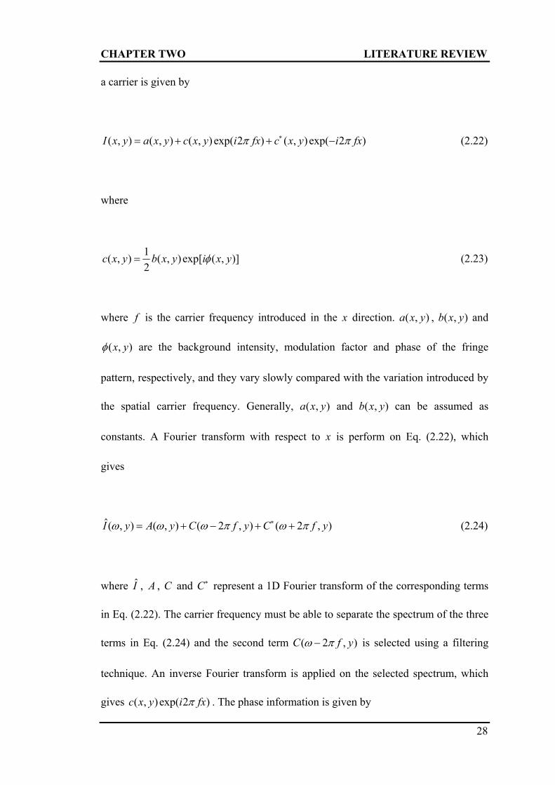
a carrier is given by
( , ) ( , ) ( , ) exp( 2 ) ( , ) exp( 2 )I x y a x y c x y i fx c x y i fx (2.22)
where
1( , ) ( , ) exp[ ( , )]
2c x y b x y i x y (2.23)
where f is the carrier frequency introduced in the x direction. ( , )a x y , ( , )b x y and
( , )x y are the background intensity, modulation factor and phase of the fringe
pattern, respectively, and they vary slowly compared with the variation introduced by
the spatial carrier frequency. Generally, ( , )a x y and ( , )b x y can be assumed as
constants. A Fourier transform with respect to x is perform on Eq. (2.22), which
gives
ˆ( , ) ( , ) ( 2 , ) ( 2 , )I y A y C f y C f y (2.24)
where I , A , C and C represent a 1D Fourier transform of the corresponding terms
in Eq. (2.22). The carrier frequency must be able to separate the spectrum of the three
terms in Eq. (2.24) and the second term ( 2 , )C f y is selected using a filtering
technique. An inverse Fourier transform is applied on the selected spectrum, which
gives ( , ) exp( 2 )c x y i fx . The phase information is given by

CHAPTER TWO LITERATURE REVIEW
29
2 ( , ) ( , ) exp( 2 )
1( , ) exp [2 ( , )]
2
fx x y angle c x y i fx
angle b x y i fx x y
(2.25)
where angle indicates taking the argument of the complex function.
Figure 2.5 shows the process of phase retrieval of a 1D signal fringe pattern
using Fourier transform method. Figure 2.5(a) shows a simulated cosine signal with a
normally distributed random noise whose variance is 0.2. Figure 2.5(b) shows its
Fourier spectrum and Fig. 2.5(c) shows a selected positive first order spectrum. Figure
2.5(d) shows the phase information of the selected positive first order spectrum
retrieved using an inverse Fourier transform. The wrapped phase values need to be
unwrapped since they are in modulus of 2 . Figure 2.5(e) shows the unwrapped
phase values which have been shifted by a specific value and the theoretical phase
values. Due to the poor noise filtering capability, fluctuations in the wrapped and
unwrapped phase values are observed in Figs. 2.5(d) and 2.5(e), respectively. In
addition, the Fourier transform is unable to provide the instantaneous frequency of a
signal, and hence more advanced methods are required to reduce the errors caused by
noise. Time-frequency analysis techniques such as CWT and WFT, which are based
on Fourier transform, with a better noise reduction capability for phase retrieval are
discussed in the following sections.

CHAPTER TWO LITERATURE REVIEW
30
Fig. 2.5 (a) A simulated intensity signal with a normally distributed random noise; (b) Fourier spectrum of the signal; (c) selected positive first order
spectrum from (b); (d) retrieved wrapped phase; (e) unwrapped phase
(a)
(c)
(b)
(d)
(e)
0 100 200 300 400 500-3
-2
-1
0
1
2
3
Pixel
Am
plit
ud
e
0 100 200 300 400 5000
50
100
150
200
250
Pixel
Am
plit
ud
e
0 100 200 300 400 5000
50
100
150
200
250
Pixel
Am
plit
ud
e
0 100 200 300 400 500-4
-2
0
2
4
Pixel
Ph
ase
(Rad
)
0 100 200 300 400 500-10
0
10
20
30
40
50
60
Pixel
Ph
ase
(Rad
)
Line 2
Line 1
Line 1: Theoretical values Line 2: Retrieved values

CHAPTER TWO LITERATURE REVIEW
31
2.2 Continuous wavelet transform (CWT) in optical measurement
The Fourier transform has the advantage that only one fringe pattern is required for
phase retrieval so that it has the potential for dynamic deformation measurement.
However, The Fourier transform is a global transform of a signal and therefore, signal
values at different points will affect each other in the processing and thus is non-
robust in noise reduction.
Unlike the Fourier transform method, CWT is a local transform with different
resolution for a signal. Therefore, CWT acts as a filter during processing and has a
better noise reduction capability than Fourier transform method (Zhong and Weng,
2005; Huang et al, 2010). Continuous wavelet transform can provide space-frequency
information synchronously while Fourier transform does not. One-dimensional
continuous wavelet transform has been widely applied to fringe analysis in optical
measurement. In 1997, Watkins et al (1997) first used CWT to accurately reconstruct
surface profiles from interferograms and compared CWT to the standard phase-
stepping method. Later, Watkins et al (1999) applied CWT to directly extract phase
gradients from a fringe pattern. Continuous wavelet transform of a fringe pattern is
able to produce the maximum modulus of wavelet transform when a daughter wavelet
is most similar to a signal in a local area. Using this method, the phase gradient of a
fringe pattern can be found and integration of the gradient will produce the phase
information. This will avoid the need for phase unwrapping. Federico and Kaufmann
(2002) applied 1D CWT method to the fringe patterns of ESPI. However this method
produces noisy phase maps if the signal to noise ratio is low and the method is not

CHAPTER TWO LITERATURE REVIEW
32
suitable for analyzing fringe patterns with horizontal and vertical spatial carriers.
Dursun et al (2004) applied Morlet wavelet to determine the phase distribution of
fringes for 3D profile measurement using a fringe projection technique. Zhong and
Weng (2004a) used CWT to retrieve the phase of the spatial carrier-fringe pattern for
3D shape measurement and overcome the limitation of Fourier transform. Watkins
(2007) also proposed a theory of the maximum modulus of a wavelet ridge for the
retrieval of an instantaneous fringe frequency, while Afifi et al (2002) employed
another wavelet, Paul wavelet, for phase retrieval from a single fringe pattern without
using phase unwrapping. The theoretical analysis of Paul wavelet algorithm was also
presented.
In addition to 1D CWT, 2D CWT has also received much attention for phase
retrieval. Compared to 1D CWT, 2D CWT has a rotation parameter in addition to the
scale parameter. The 1D CWT is able to retrieve phase values correctly from a fringe
pattern with high signal to noise ratio. For a noisy fringe pattern (for example, a fringe
pattern with speckle noise), 1D CWT will produce a noisy wrapped phase map which
will affect the success rate of the phase unwrapping algorithms and may fail to
produce a continuous phase map. It is unable to obtain the correct integral multiples
of 2 for the wrapped phase map in this case. Furthermore, 1D CWT is not suitable
for analyzing a fringe pattern with spatial frequencies in the vertical and horizontal
directions, while the 2D CWT is suitable since processing is in two dimensions.
Kadooka et al (2003) first employed 2D CWT for analyzing a moiré interference
fringe pattern. This technique overcame the difficulty of phase retrieval encountered

CHAPTER TWO LITERATURE REVIEW
33
by the Fourier transform method. In 2006, Gdeisat et al (2006) proposed to use a 2D
fan CWT algorithm to demodulate phase values from a noisy fringe pattern.
Compared to the 1D CWT, the 2D fan CWT algorithm showed an improvement of
noise reduction. However, there were still fluctuations affected by noise in the phase
map and the method failed to show correct phase values from some speckle fringe
patterns due to the narrow bandwidth of the 2D fan wavelet. In 2006, Wang and Ma
(2006) also proposed an advanced CWT algorithm for phase retrieval from a fringe
pattern using microscopic moiré interferometry. This method produces better results
than the 1D CWT.
Two approaches, namely phase estimation from wavelet coefficients and
frequency estimation from the ridge of wavelet transform are used for phase retrieval.
In the former case, the CWT is used to calculate the correlation between the fringe
pattern and the wavelet functions with different scale parameters. When the wavelet
function is most similar to the signal in a local area of the fringe pattern, the modulus
of the wavelet transform coefficient will reach a maximum value. The phase
information can thus be retrieved from the real and imaginary part of the wavelet
transform coefficient when its modulus reaches a maximum value. Phase retrieval
from the former approach is more accurate, but phase unwrapping is required to
remove 2 jumps in a wrapped phase map. For the latter approach, since phase is
retrieved from integration of an instantaneous frequency of the fringe pattern, phase
unwrapping is avoided. However, the accuracy of this technique depends on the scale
resolution. A high scale resolution will increase the computation time. Furthermore,

CHAPTER TWO LITERATURE REVIEW
34
integration of the instantaneous frequency will propagate phase error from one pixel
to its adjacent pixel. Therefore, the former approach is more commonly used.
Complex wavelet such as Morlet wavelet is commonly used in optical
measurement for phase retrieval. Figure 2.6(a) shows a plot of a 1D Morlet wavelet
and its spectrum. The scale of the Morlet wavelet is 1 and 0 is 2 . The upper half
of Fig. 2.6(a) shows the real and imaginary parts of the Morlet wavelet which are
represented by the solid and dash lines, respectively. The lower half shows its Fourier
spectrum. Since a complex Morlet wavelet contains the phase information in its real
and imaginary parts, it is used for phase retrieval of the signal from their similarity.
The 1D CWT of a signal is defined as (Mallat, 2001; Zhong and Weng, 2005;
Watkins, 2007)
1
21( , ) ( ) ( )d
x mWf q m q f x dx
q
(2.26)
where 1 ( )df x represents a signal and the symbol represents complex conjugation.
( )x m
q
denotes a wavelet function with translation on the x -axis by m and
dilation by scale q ( 0q ) of the mother wavelet ( )x , which is usually a complex
Morlet wavelet function given by
1 24
0( ) exp( )exp( )2
xx i x
(2.27)

CHAPTER TWO LITERATURE REVIEW
35
where 0 is a fixed frequency and can be set as 2 to meet the admissibility
condition. As can been seen, the coefficients ( , )Wf q m of wavelet transform is able to
provide spatial and frequency information simultaneously. A wavelet ridge is a path
that follows the maximum values of ( , )Wf q m from which the phase and
instantaneous frequency can be obtained. To use a 1D CWT for phase retrieval from a
fringe pattern, the 1D signal of a fringe pattern described by Eq. (2.22) is given by
1 1( ) exp [ ( ) 2 ] exp [ ( ) 2 ]
2 2I x a b i x fx b i x fx (2.28)
where the background intensity a and the modulation factor b are considered as
constants. Assuming that the 1D intensity signal has a linear phase change, which can
be easily achieved in the experiment, the phase term may be expanded using Taylor
series of the first order and given by
( ) ( ) '( )( )x m m x m (2.29)
hence the 1D CWT of Eq. (2.28) is given by
1
2
1 2 3
( , ) ( ) ( )
( , ) ( , ) ( , )
x mWf q m q I x dx
q
Wf q m Wf q m Wf q m
(2.30)
where

CHAPTER TWO LITERATURE REVIEW
36
1 204
1
2104
2
2104
3
( , ) 2 exp( )2
[2 '( )]( , ) exp [ ( ) 2 ] exp
2 2
[2 '( )]( , ) exp [ ( ) 2 ] exp
2 2
Wf q m qa
f m qqWf q m b i m fm
f m qqWf q m b i m fm
(2.31)
From Eq. (2.31) it can be seen that when the scale parameter q of the CWT satisfies
the following equation
0
2 '( )q
f m
(2.32)
the modulus of CWT becomes
2( , ) ( , )Wf q m Wf q m (2.33)
since 1( , ) 0Wf q m and 3( , ) 0Wf q m . The normalized scalogram represented by
2( , )Wf q m
q will yield a maximum value. For phase retrieval, the maximum value of
( , )Wf q m is used to determine the wavelet ridge. Therefore, instantaneous frequency
of the fringe pattern can be retrieved from Eq. (2.32). Furthermore, phase information
can be retrieved from 2 ( , )Wf q m which is given by

CHAPTER TWO LITERATURE REVIEW
37
( , )( ) 2
( , )
Im Wf q mm fm arctan
Re Wf q m
(2.34)
where Im represents the imaginary part of ( , )Wf q m , Re represents the real part of
( , )Wf q m . As can be seen from Fig. 2.6(b), a scalogram of ( , )Wf q m for the signal
shown in Fig. 2.5(a) can be obtained. The dash line represents the ridge of CWT. As
can be seen from this scalogram, both spatial and frequency information of the signal
can be obtained from CWT. Therefore, CWT has the advantage over Fourier
transform which can only provide the frequency information of the signal. Figure
2.6(c) shows the unwrapped phase using CWT. The top line shows the theoretical
phase values and the bottom line shows the phase values obtained from Eq. (2.34)
after unwrapping. For clarity, the calculated phase values are shifted by a certain
offset. As can be seen, the retrieved phase values closely approximates to the
theoretical values. The noise of an intensity signal is suppressed using the 1D CWT
and the result obtained is smoother than that of the Fourier transform. The reason is
that the modulus of the wavelet transform coefficient of the noise is less than that of
the signal and can be suppressed during the processing.
Two-dimensional wavelet transform has also been proposed for phase retrieval
from a fringe pattern in 3D profile measurement. The processing is in two dimensions
and the theory is presented in detail in Chapter three.

CHAPTER TWO LITERATURE REVIEW
38
Morlet wavelet: 1scale , 0 2
-10 -5 0 5 10-1
0
1
-10 -5 0 5 100
1
2Spectrum
Real part
Imaginary part
(a)
Fig. 2.6 (a) A 1D Morlet wavelet and its spectrum; (b) a scalogram of
( , )Wf q m for the signal shown in Fig. 2.5(a) and the dash line represents the
ridge of CWT; (c) unwrapped phase using CWT
(b)
(c)
0 100 200 300 400 500-10
0
10
20
30
40
50
60
Pixel
Ph
ase
(Rad
)
Line 2
Line 1
Line 1: Theoretical values Line 2: Retrieved values

CHAPTER TWO LITERATURE REVIEW
39
2.3 Windowed Fourier transform (WFT) in optical measurement
Unlike CWT, which has a variable resolution for time-frequency analysis, WFT has a
fixed resolution in both time and frequency domain during processing once a window
size is selected, according to the uncertainty principle. Figure 2.7 shows different
basis for different time-frequency transform. As can be seen, for different frequencies,
the Fourier basis is always continuous which means it is a transform for a global
signal, while the wavelet basis is dilated or compressed with different resolutions in
both time and frequency domain and the transform is applied on a local signal within
a window. As for the WFT, the transform has a fixed resolution for all the frequency
components and it is also a transform of a local signal within a window.
Fig. 2.7 Basis of transform for time-frequency analysis
Wavelet basis
Fourier basis
Windowed Fourier basis

CHAPTER TWO LITERATURE REVIEW
40
In 2002, Wang and Asundi (2002) applied the Gabor filter for strain
contouring and employed the theory of WFT for phase retrieval. In addition, Qian
(2004, 2007b) proposed WFT and 2D WFT as an alternative method for phase
retrieval and fringe demodulation and obtained satisfactory results. However, the
algorithm was employed using the convolution theory which resulted in a long
computational time. Other researchers such as Zhong and Weng (2004b) have
proposed a dilating Gabor transform for 3D shape measurement. Multi-scale WFT for
phase extraction was also proposed by Zhong and Zeng (2007). An adaptive WFT for
3D shape measurement was also proposed by Zheng et al (2006). Gao et al (2009)
employed a real-time 2D parallel system for WFT to show the potential of WFT for
real-time phase retrieval.
Similar to CWT, phase can also be retrieved from either coefficient or
instantaneous frequency of WFT. However, phase retrieved from the integration of
instantaneous frequency, namely phase derivative, normally results in a larger error
compared with the phase retrieved from the coefficient of WFT. In WFT, there are
two most frequently used methods called WFF method and windowed Fourier ridges
method (Qian, 2004; Qian, 2007b). Both methods can be applied to a fringe pattern
with speckle noise for noise reduction and phase retrieval. Using WFT for fringe
demodulation, both spatial and frequency information can be simultaneously obtained
and the parameters of WFT should also be correctly selected.
The 1D WFT and 1D inverse WFT of Eq. (2.28) are given by
CHAPTER TWO LITERATURE REVIEW
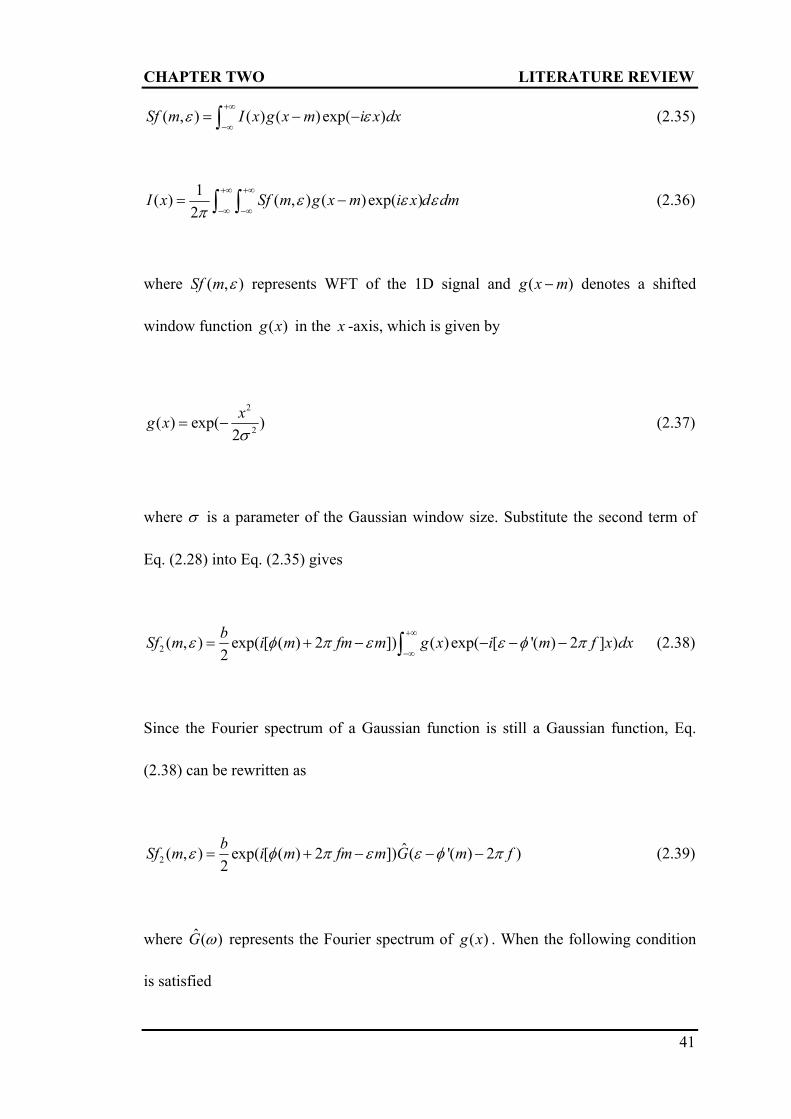
41
( , ) ( ) ( ) exp( )Sf m I x g x m i x dx
(2.35)
1( ) ( , ) ( ) exp( )
2I x Sf m g x m i x d dm
(2.36)
where ( , )Sf m represents WFT of the 1D signal and ( )g x m denotes a shifted
window function ( )g x in the x -axis, which is given by
2
2( ) exp( )
2
xg x
(2.37)
where is a parameter of the Gaussian window size. Substitute the second term of
Eq. (2.28) into Eq. (2.35) gives
2 ( , ) exp( [ ( ) 2 ]) ( )exp( [ '( ) 2 ] )2
bSf m i m fm m g x i m f x dx
(2.38)
Since the Fourier spectrum of a Gaussian function is still a Gaussian function, Eq.
(2.38) can be rewritten as
2ˆ( , ) exp( [ ( ) 2 ]) ( '( ) 2 )
2
bSf m i m fm m G m f (2.39)
where ˆ ( )G represents the Fourier spectrum of ( )g x . When the following condition
is satisfied

CHAPTER TWO LITERATURE REVIEW
42
'( ) 2m f (2.40)
the WFT modulus ( , )Sf m of Eq. (2.28) can be approximated as 2 ( , )Sf m , since
the WFT modulus of the first and third term of Eq. (2.28) are approximate to zero.
The WFT modulus ( , )Sf m will reach the maximum value when Eq. (2.40) is
satisfied. Therefore, the filtered phase information is retrieved as
2( ) 2 exp( ) ( , )m fm angle i m Sf m (2.41)
where symbol ‘ ’ represents a filtering operation. This method is the windowed
Fourier ridges method for phase retrieval. Another method, WFF can also be used for
phase retrieval and is given by
1( ) [ ( ) ( , )] ( , )
2
h
lI x I x D x D x d
(2.42)
where
( , ) ( ) exp( )D x g x i x (2.43)
Symbol represents a convolution operation and [ ( ) ( , )]I x D x denotes the
filtered value of ( ) ( , )I x D x using a threshold value, while ( )I x denotes the
filtered value of ( )I x with integration limits from l to h . The filtered phase value

CHAPTER TWO LITERATURE REVIEW
43
can be retrieved using
( ) 2 ( )x fx angle I x (2.44)
Similar to CWT, the windowed Fourier ridges method is able to retrieve the
instantaneous frequencies of a fringe pattern and provide phase information without
phase unwrapping by integration of the instantaneous frequencies. However, this
approach also has a limitation as the accuracy of the retrieved phase is restricted by
the integration step and phase values retrieved from instantaneous frequencies
normally incur a large error. In addition, the phase values can be directly retrieved
from the coefficients of the windowed Fourier ridges and this approach is more
accurate than the integration of the instantaneous frequencies. Besides, the WFF
method is also an important method of WFT for phase retrieval. The principle of WFF
is similar to the filtering using Fourier transform. The intensity of a fringe pattern is
transform to a windowed Fourier domain and a threshold is used to filter the
windowed Fourier spectrum. Then the filtered spectrum is transformed back using an
inverse WFT and the filtered phase information can be retrieved by taking the
argument of the result.
Two-dimensional windowed Fourier transform which has the advantages over
1D CWT and 1D WFT for fringe demodulation because the processing is in both the
x and y directions of a fringe pattern has received more attention recently. It is
suitable for phase retrieval since fringe patterns normally have variations in both the

CHAPTER TWO LITERATURE REVIEW
44
x and y directions. Since WFT is a local transform of a signal, the advantage is that
signals within the window will not be affected by other signals outside the window.
Therefore, WFT has been widely applied in fringe demodulation obtained from
interferometry. Moreover, unlike CWT, the temporal and frequency resolution of
WFT is always the same during processing once the window size is selected and the
resolution can be selected according to the spectrum of a fringe pattern even at very
low frequencies. In CWT, the resolution at very low frequencies is very high which
means the wavelet window in frequency domain is very narrow around that frequency,
it will not be possible to acquire enough information for phase retrieval at the low
frequency and may result in failure for phase retrieval. Moreover, a large wavelet
scale is required for low frequency and this will incur a large amount of processing
time for a wide scale range. Therefore, CWT is not suitable for demodulation of low
frequency fringe patterns. Previous WFT method using convolution algorithm
requires a large amount of computation time due to the integration step and window
size. This is a limitation of the WFT and therefore, the present study is focused on
improving its computation efficiency.

CHAPTER THREE DEVELOPMENT OF THEORY
45
CHAPTER THREE
DEVELOPMENT OF THEORY
This chapter focuses on the theoretical development of the proposed optical phase
retrieval algorithms. The first section covers theoretical development of 2D Gabor
CWT. Limitations of previous 2D CWT are discussed. Previous 2D fan CWT is
compared and the advantage of the proposed wavelet transform algorithm is discussed.
In the second section, an improved WFT algorithm is proposed for phase retrieval and
noise reduction of a speckle fringe pattern. Limitations of the WFT with convolution
algorithm are emphasized. The Gerchberg extrapolation method is used to suppress
the boundary effect. The last section is devoted to phase fringe denoising using the
WFF method. A single wavelength DSSI based on WFF and a two-wavelength DSSI
based on sine-cosine filtering are compared. A two-wavelength technique with a
combined filtering method for phase retrieval in DSSI is also proposed. The method
exploits the advantages of a two-wavelength technique as an alternative to phase
unwrapping.
3.1 Two-dimensional (2D) CWT for phase retrieval
Two-dimensional continuous wavelet transform has been applied to digital image
analysis (Antoine et al, 1993). Since an interference pattern can be presented in a
digital format, digital image processing techniques, such as 2D CWT, can be

CHAPTER THREE DEVELOPMENT OF THEORY
46
employed for fringe demodulation. The 2D CWT of a fringe pattern ( )I X with
respect to a 2D wavelet ( ) X is given by (Wang and Ma, 2006; Antoine et al, 1993)
2 2 1( , , ) [ ( )] ( )WT q q d q r I t tb X X b X (3.1)
where the symbol “ ” represents an operation of complex conjugate, ( , )x yX
represents the spatial coordinates of the fringe pattern, ( , )x yb btb denotes a
translation parameter along two coordinate axes, q is a scale dilation parameter, r
is a rotation matrix of size 22 and is a rotation angle. The rotation matrix r
which acts on ( , )x yX is given by
( cos sin , sin cos )r x y x y X (3.2)
In addition, the 2D CWT can also be defined in the frequency domain as
2 ˆˆ( , , ) exp( ) ( )WT q d i qr I t tb K b K K K (3.3)
where ( , )x y K denotes the frequency coordinates, x x y yb b tb K is an
Euclidean scalar product, and “ ^ ” denotes a Fourier spectrum. Using Eq. (3.3), the
computation efficiency can be improved significantly since fast Fourier transform is
introduced.

CHAPTER THREE DEVELOPMENT OF THEORY
47
3.1.1 Limitations of previous 2D CWT
In fringe pattern analysis, a commonly used mother wavelet for phase retrieval and
fringe filtering is a complex Morlet wavelet. In fact, the complex Morlet wavelet is a
special case of a complex Gabor wavelet. Figure 3.1 shows a 2D complex Morlet
wavelet. The real part, imaginary part and Fourier spectrum of the 2D complex Morlet
wavelet with a rotation angle 2
are shown in Figs. 3.1(a), 3.1(b) and 3.1(c),
respectively.
The mathematical expression of 2D Morlet wavelet is given by
21( ) exp( )exp
2M i
0X K X X (3.4)
where 0( ,0)k0K is the central frequency of a 2D Morlet wavelet, and therefore
0k x 0K X . As can be seen, the complex Morlet wavelet has a Gaussian envelop.
Fig. 3.1 (a) Real part of a 2D Morlet wavelet; (b) imaginary part of a 2D Morlet wavelet; (c) Fourier spectrum of a 2D Morlet wavelet
(a) (b) (c)

CHAPTER THREE DEVELOPMENT OF THEORY
48
The real and imaginary parts vary in the form of a cosine and sine function,
respectively. Therefore, the complex Morlet wavelet can be used to analyze the fringe
variation for phase retrieval. However, in CWT, the frequency resolution for a low
frequency component is very high and would result in a narrow frequency window,
while for a high frequency component it would result in a wide frequency window.
Therefore, the 2D complex Morlet wavelet has a narrow spectrum for a low frequency
component (Gdeisat et al, 2006; Kadooka et al, 2003). It is only suitable for phase
retrieval from a fringe pattern with a narrow bandwidth and will fail to demodulate
fringe patterns with wide bandwidths in the spectrum.
Besides the 2D complex Morlet wavelet, 2D fan CWT has also been used for
fringe analysis (Gdeisat et al, 2006). A 2D fan wavelet is constructed by superposing
a number of complex Morlet wavelets. Similar to the 2D complex Morlet wavelet, it
fails to demodulate fringe patterns with a wide bandwidth and high speckle noise. To
overcome this problem, one possible solution is to introduce a window extension
parameter in a 2D fan wavelet. An advanced 2D fan wavelet with a rotation angle
is given by
1
2 202
0
1exp ( ) [ cos( ) sin( )]
2
N
Fan t tt
r x y ik x y
X (3.5)
The Fourier transform of Fan r X is given by

CHAPTER THREE DEVELOPMENT OF THEORY
49
1
2 2 20 0
0
1ˆ exp [ cos( )] [ sin( )]
2
N
Fan x t y tt
r k k
K (3.6)
where tt , 30 and N=6 is the number of superposed Morlet wavelets (Kirby,
2005). Figure 3.2 shows a 2D fan wavelet. The real part, imaginary part and Fourier
spectrum of the 2D fan wavelet with a rotation angle 3
are shown in Figs.
3.2(a), 3.2(b) and 3.2(c), respectively. As can be seen from the spectrum, there are six
bumps which represent six Morlet wavelets.
With an advanced 2D fan wavelet, the frequency window for processing the
low frequency components can be enlarged, however, because of the superposition of
several complex Morlet wavelets, the spectrum in the frequency domain is wider and
thus results in more spatial noise which will degrade the retrieved phase.
Fig. 3.2 (a) Real part of a 2D fan wavelet; (b) imaginary part of a 2D fan wavelet; (c) Fourier spectrum of a 2D fan wavelet
(a) (b) (c)

CHAPTER THREE DEVELOPMENT OF THEORY
50
3.1.2 Advanced 2D Gabor CWT
To overcome this problem, a suitable wavelet function should be selected. A 2D
complex Gabor wavelet can be used since it has a controllable Gaussian window in
both the spatial and frequency domains. This character makes its frequency resolution
for the low frequency components adjustable using a parameter for window size
control. A 2D complex Gabor wavelet is given by
2
2
1( ) exp( )exp
2G i
0X K X X (3.7)
where is a parameter for controlling the window size. is 0.5 (Wang and Ma,
2006) and 0k is 5.336 (Gdeisat et al, 2006) in this study. 0k and are able to control
the window size in both the spatial and frequency domain. The parameter 0k controls
the central frequency and determines the window size at that frequency. The
Fourier transform of 2D Gabor wavelet is given by
22ˆ ( ) exp
2G
0K K K (3.8)
The 2D Gabor wavelet shows similar images with those of the 2D Morlet wavelet
shown in Fig. 3.1. Unlike the 2D Morlet wavelet, the 2D Gabor wavelet is suitable for
analyzing a fringe pattern with a narrow or wide bandwidth in the frequency domain.
This is because the window size of a 2D Gabor wavelet for a low frequency

CHAPTER THREE DEVELOPMENT OF THEORY
51
component can be extended using the parameter . Thus more useful information
can be obtained since the low frequency region contains most of the energy of the
signal. A suitable value of should be selected to obtain useful information and
reduce the spatial noise in a noisy fringe pattern. The 2D Gabor wavelet
1[ ( )]G q r tX b with a translation parameter tb , a dilation parameter q (q > 0) and
a rotation angle is given by
2 21
2 2
0
[( ) ( ) ]1[ ( )] exp
2
[( ) cos ( )sin ]
x yG
x y
x b y bq r
q
x b y bik
q
tX b
(3.9)
hence ˆG qr
K is given as
2 2 20 0
1ˆ exp [( cos ) ( sin ) ]
2G x yqr q k q k
K (3.10)
The following section discusses the use of 2D Gabor CWT for phase retrieval from a
speckle fringe pattern with a spatial carrier. A local speckle fringe pattern with a
spatial carrier is given by (Wang and Ma, 2006)
0 1
( ) cos ( )sin( ) cos 2 x yl
l l
x b y bI I I
P
X (3.11)

CHAPTER THREE DEVELOPMENT OF THEORY
52
where xb and yb denote translation parameters of tb in the fringe pattern, P is a local
fringe period, is a local fringe direction, is an unknown phase to be retrieved, 0lI
and 1lI considered as constants are background intensity and modulation factor,
respectively. The Fourier spectrum of Eq. (3.11) is given by
20
21
21
[ ( )] 4 ( , )
22 exp( )exp ( cos sin )
2 2cos , sin
22 exp( )exp ( cos sin )
2 2cos , sin
ll x y
l x y
x y
l x y
x y
F I I
I i i b bP
P P
I i i b bP
P P
X
(3.12)
where F denotes the Fourier transform, is the Dirac function. In Eq. (3.12) the
direct current term (zero-frequency term) and two side-frequency components are
separated by the carrier. Therefore, the direct current term and the left side-frequency
component in the frequency domain are first removed for phase extraction to remove
their interference. Eq. (3.12) then becomes
21
2[ ( )] 2 exp( )exp ( cos sin )
2 2cos , sin
lremoved l x y
x y
F I I i i b bP
P P
X
(3.13)
The 2D Gabor CWT is then employed to process the right side-frequency component.

CHAPTER THREE DEVELOPMENT OF THEORY
53
Substitute Eq. (3.10) and Eq. (3.13) into Eq. (3.3), the 2D Gabor CWT becomes
21
2 22
0 0
( , , ) 2 exp( )
1 2 2exp cos cos sin sin
2
llWT q I i
q k q kP P
tb
(3.14)
where ( , , ) ( , , )lWT q WT q t tb b denotes the wavelet transform of the whole fringe
pattern for a translation tb . This is equivalent to the wavelet transform of the local
fringe pattern for a translation tb . In Eq. (3.12), a rectangular window is employed to
select the second term from the spectrum of the fringe pattern and an inverse Fourier
transform is performed. The phase value can then be obtained by removing the spatial
noise outside the rectangular window. However, this method is only suitable for a
fringe pattern with less noise. In addition, the rectangular window used is not optimal
for a circular spectrum and it is not easy to determine the window size automatically.
Using a maximum modulus algorithm of the 2D Gabor CWT, Eq. (3.14) becomes
21max
2 2 20 0
( , , ) max 2 exp( )
1 2 2exp ( cos cos ) ( sin sin )
2
llWT q I i
q k q kP P
tb
(3.15)
In Eq. (3.15), when the local fringe direction and period are respectively equal to the
wavelet direction and period multiplied by a constant, i.e. and 0( / 2 )q k P ,
the modulus in Eq. (3.15) will reach its maximum value and is much greater than the

CHAPTER THREE DEVELOPMENT OF THEORY
54
modulus of the wavelet transform of the noise, hence the phase value can be
retrieved from Eq. (3.14) using the maximum modulus method of the wavelet
transform. In the 2D Gabor CWT, the integration in Eq. (3.1) analyzes the local
similarity between the 2D Gabor wavelets and the fringe pattern. The wavelets are
dilated and rotated during processing. Wavelet transform is a local transform to
measure the similarity between a daughter wavelet and the fringe pattern in a local
region. When the wavelet and the fringe pattern are locally most similar, the modulus
of the 2D CWT reaches its maximum value for a particular value of translation along
the horizontal and vertical axis in the fringe pattern. Using the complex wavelet,
phase information of the fringe pattern can be obtained from the real and imaginary
parts of the wavelet transform.
Therefore, the 2D Gabor CWT algorithm shows a better speckle noise
reduction capability than the 2D Fourier transform with a rectangular window filter.
In this study, Eq. (3.14) is multiplied by the scale dilation parameter q and then the
maximum modulus algorithm is employed to retrieve the phase. The parameter q
does not affect the maximum modulus algorithm due to the exponential function of
Eq. (3.14). This approximation shows a better noise reduction capability in the 2D
Gabor CWT.
It should be noted that in the 2D Gabor CWT, the frequency window of the
wavelet transform for a high frequency component is larger than that for a low
frequency component, hence more noise will be introduced for a large frequency

CHAPTER THREE DEVELOPMENT OF THEORY
55
window even though it is able to obtain more useful signals. A suitable window
extension parameter should be selected to provide an optimal window. Normally,
is recommended as an initial value of 0.5 (Wang and Ma, 2006).
3.2 Improved WFT for fringe demodulation
Unlike CWT, WFT has a fixed resolution for signal processing once a window size is
selected. Therefore, the frequency window of a windowed Fourier element remains
constant for either a high or low frequency component. It is a suitable method for
demodulating a fringe pattern with either a wide or narrow spectrum due to the
controllable time-frequency resolution.
3.2.1 Limitations of WFT with convolution algorithm
Windowed Fourier transform applied to phase retrieval has shown a good noise
reduction capability. However, the WFT with convolution algorithm which is affected
by the window size, image size and interval of the integration is time consuming. The
intensity ),( yxI of an interference fringe pattern can be expressed by Eq. (2.1).
Similar to the 1D WFT, the 2D WFT and 2D inverse WFT of a fringe pattern using a
convolution operation are given by
,( , , , ) [ ( , ) ( , )]exp( )Sf m n I m n D m n i m i n (3.16)
, ,2
1( , ) [ ( , ) ( , )] ( , )
4I x y I x y D x y D x y d d
(3.17)

CHAPTER THREE DEVELOPMENT OF THEORY
56
where
2 2
, 2( , ) exp exp
2
x yD x y i x i y
(3.18)
and , ( , )D x y represents the window element of the WFT. A filtered phase value can
be retrieved using 2D windowed Fourier ridges or 2D WFF method (Qian, 2007b).
Using the WFF with convolution algorithm, the computation time for phase retrieval
from a fringe pattern of 512 512 pixels will be a few minutes and hence, the
computation efficiency should be enhanced.
3.2.2 Phase retrieval using improved WFT
To reduce the computation time for phase retrieval, an improved algorithm of WFT is
proposed. The algorithm is based on the introduction of a fast Fourier transform in
WFT and able to avoid the window size effect on computation time. Windowed
Fourier transform method includes windowed Fourier ridges method and WFF
method. Theoretical analysis of the improved windowed Fourier ridges method and
WFF method is proposed.
In Eq. (3.18), the window element of the WFT shows a Gaussian envelop and
the Fourier spectrum of Eq. (3.18) is given by

CHAPTER THREE DEVELOPMENT OF THEORY
57
2 2 22
,
[( ) ( ) ]ˆ ( , ) 2 exp2
x yx yD
(3.19)
where “ ^ ” denotes the Fourier spectrum. x and y are frequencies along the x - and
y -axis, respectively. The constant factor 22 can be ignored for the given factor
since it only affects the amplitude of the WFT except the phase. According to the
convolution theorem (Mallat, 2001), convolution can easily be performed using
frequency-domain multiplication by the fast Fourier transform, hence Eq. (3.16) can
be written as
1,
ˆ ˆ( , , , ) exp( ) [ ( , ) ( , )]x y x ySf m n i m i n F I D (3.20)
where ),(ˆ yxI is the Fourier transform of ),( yxI and 1F denotes an inverse
Fourier transform operation. Thus, Eq. (3.17) can be re-written as
1 1, ,2
1 ˆ ˆ ˆ( , ) { [ ( , ) ( , )]} ( , )4 x y x y x yI x y F F F I D D d d
(3.21)
where F denotes a Fourier transform operation. Furthermore, the phase ( , )x y can
be expressed as
1 2( , ) ( , ) ( , )( ) ( , )( )x y m n m n x m m n y n (3.22)

CHAPTER THREE DEVELOPMENT OF THEORY
58
where ( , )m n , ),(1 nm and ),(2 nm are respectively the phase value, frequency
along the x - and y -axis at a point 0 ( , )M m n . The coordinate ( , )m n is omitted for
simplification. Thus ),(ˆ yxI is given as
2
21 2 1 2
21 2 1 2
ˆ( , ) 4 ( , )
2 exp[ ( )] ( , )
2 exp[ ( )] ( , )
x y x y
x y
x y
I a
b i m n
b i m n
(3.23)
where is a Dirac function. In Eq. (3.23) the direct current term and two side-
frequency components are separated by the carrier. The direct current and the left
side-frequency components in the frequency domain are first removed to reduce their
effect on phase retrieval from the right side-frequency component, and hence Eq.
(3.23) becomes
21 2 1 2
ˆ ( , ) 2 exp[ ( )] ( , )r x y x yI b i m n (3.24)
Substituting Eq. (3.24) into Eq. (3.20), we have
2, 1 2
ˆ( , , , ) exp[ ( )]2 exp( ) ( , )Sf m n i m n b i D (3.25)
The phase values are contained in Eq. (3.25) and can be retrieved from the
following equation

CHAPTER THREE DEVELOPMENT OF THEORY
59
1 2,
exp[ ( )] ( , , , )angle i m n Sf m n
(3.26)
The modulus of ),,,( nmSf would reach a maximum value when 21, is
satisfied. The phase value for the coefficient of ),,,( nmSf with a maximum
modulus is equal to the phase of the fringe pattern. Phase retrieval from the ridges of
the ),,,( nmSf is termed windowed Fourier ridges method. In Eq. (3.20), the fast
Fourier transform is employed and the computation efficiency is improved for the
windowed Fourier ridges method. In the WFF method, the phase can be obtained
by substituting Eq. (3.24) into Eq. (3.21). The filtered values of ),( yxI using the
WFF method is given by
1 1, ,2
1 ˆ ˆ ˆ( , ) [ ( , ) ( , )] ( , )4
h h
r x y x y x yl lI x y F F F I D D d d
(3.27)
where l , h and l , h are the integration limits of and , respectively, and
1,
1 1, ,
1,
ˆ ˆ[ ( , ) ( , )]
ˆ ˆ ˆ ˆ[ ( , ) ( , )] if [ ( , ) ( , )] threshold
ˆ ˆ0 if [ ( , ) ( , )] threshold
r x y x y
r x y x y r x y x y
r x y x y
F I D
F I D F I D
F I D
(3.28)
where 1,
ˆ ˆ[ ( , ) ( , )]r x y x yF I D denotes the filtered values of
1,
ˆ ˆ[ ( , ) ( , )]r x y x yF I D using a threshold value. Only the modulus of
1,
ˆ ˆ[ ( , ) ( , )]r x y x yF I D which is greater than or equal to the threshold value is

CHAPTER THREE DEVELOPMENT OF THEORY
60
retained, otherwise it is set as zero. Using this method, speckle noise can be
suppressed. The phase values are given by
( , )angle I x y (3.29)
where ( , )I x y denotes a filtered fringe pattern, hence with the fast Fourier transform
employed, the computation time using the WFF method is reduced significantly.
3.2.3 Suppression of boundary effect
With the introduction of fast Fourier transform in the WFT, the computation time for
fringe demodulation can be reduced significantly. However, the Fourier transform of
the fringe pattern is influenced by the boundary effect. To overcome this problem, the
Gerchberg extrapolation method (Gerchberg, 1974; Roddier C. and F. Roddier, 1987;
Chen et al, 2007) is employed to extrapolate the fringe pattern at each boundary
(using 20 pixels). After applying the proposed WFT to the extrapolated fringe pattern,
the desired area on a retrieved phase map can be obtained by removing the boundary.
Before the Gerchberg method is employed, a fringe pattern is pre-processed to retain
its grey value in the range of [-v, +v], where v is the maximum grey value (chosen as
127.5 in this study). Figure 3.3 shows a flow chart of the Gerchberg extrapolation
method. The processed fringe pattern is padded with zeros at each boundary (with 20
pixels) and the fast Fourier transform is then applied to obtain the Fourier spectrum.
The zero frequency and two-side lobes are then selected. Frequencies outside the

CHAPTER THREE DEVELOPMENT OF THEORY
61
selected areas in the Fourier spectrum are set to zeros. An inverse Fourier transform
of this Fourier spectrum would produce a fringe pattern with the extrapolated fringes.
The values within the extrapolated fringe pattern are replaced by the original values.
Another fast Fourier transform is then performed on the newly generated fringe
pattern and the whole procedure is repeated. After N iterations, the desired
extrapolated fringe pattern is obtained. In this study, ten iterations are required to
obtain a satisfactory fringe pattern.
An example of the fringe extrapolation using this technique is shown in Fig.
3.4. After 10 iterations, an extrapolated speckle fringe pattern from the original
speckle fringe pattern is obtained. It should be noted that the Gerchberg extrapolation
method requires a proper selection of the Fourier spectrum.
Extrapolated interferogram
Interferogram (average value is removed and the
interferogram is padded with zeros at the boundaries)
Fast Fourier transform
Values outside the selected areas in the Fourier spectrum are
set to zeros
Inverse fast Fourier transform
Original values are put back into the interferogram
After N iterations
Fig. 3.3 Flow chart of the Gerchberg extrapolation method

CHAPTER THREE DEVELOPMENT OF THEORY
62
3.3 Phase fringe denoising using windowed Fourier filtering
Speckle noise reduction is an important aspect in the WFF method. Since speckle
noise always appears in laser interferograms, it is necessary to suppress the speckle
noise for accurate measurement. Moreover, speckle noise reduction in a phase fringe
pattern is often necessary since the noise will affect the spatial phase unwrapping
techniques to obtain a correct continuous phase map. For relatively large deformation
measurement, wrapped phase maps are usually dense and conventional sine-cosine
average filtering technique is difficult to reduce the noise in such a case. In this
Fig. 3.4 An example of fringe extrapolation
Fast Fourier transform Zero padding after
subtracting average value
Inverse fast Fourier transform
Frequency selection
Final extrapolated fringe pattern
10 iterations

CHAPTER THREE DEVELOPMENT OF THEORY
63
section, the WFF method is proposed to reduce speckle noise in wrapped phase maps
for deformation measurement.
3.3.1 Phase retrieval for relatively large deformation measurement
Digital speckle shearing interferometry is widely employed to determine the
deformation derivative. However, for relatively large deformation measurement using
single wavelength illumination, the iterative sine-cosine average filtering (ISCAF)
method, which is a commonly used filtering technique for noise reduction, is no
longer suitable to filter the wrapped phase pattern correctly. The ISCAF technique
only works well in phase fringe patterns which are relatively less dense, hence the
measurement range is limited especially when a single wavelength is used. Since the
WFF technique shows a good potential in noise reduction for phase retrieval from a
noisy fringe pattern, it is proposed to reduce speckle noise of a dense phase fringe
pattern for relatively large deformation measurement using single wavelength
illumination in DSSI.
3.3.1.1 Windowed Fourier filtering
Using Carré algorithm, four interferograms are recorded with the phase between two
consecutive interferograms shifted by a constant amount. The phase is retrieved using
Eq. (2.19). The phase value at each point in the interferogram before and after the
object deformation ( b and a ) can be obtained and the phase difference is given
by

CHAPTER THREE DEVELOPMENT OF THEORY
64
4 xa b
w
x
(3.30)
where is the wavelength used, x is a shear value in the x-direction, w is the out-
of-plane deformation and xw / is the derivative of out-of-plane deformation. As
is in modulo of 2 , it needs to be unwrapped. However, speckle noise contained
in the phase map of requires to be suppressed before phase unwrapping. The
phase deference obtained from Eq. (3.30) can be represented using the complex form
by
1( , ) exp[ ( , )]P x y i x y (3.31)
where 1( , )P x y represents the unfiltered complex phase values. Applying the WFF
method using Eqs. (3.27) and (3.28), the filtered phase difference is given by
1( , ) ( , )x y angle P x y (3.32)
while 1( , )P x y indicates the filtered values of 1( , )P x y . The filtered phase fringe
pattern ( , )x y representing the measurand can then be unwrapped correctly using
spatial phase unwrapping (Ghiglia and Pritt, 1998).

CHAPTER THREE DEVELOPMENT OF THEORY
65
3.3.1.2 Iterative sine-cosine average filtering
Since the WFF method requires correct parameters for noise reduction and phase
retrieval, it is complicated to use compared with the ISCAF method. The ISCAF
technique was employed by Aebischer and Waldner (1999) for speckle noise
suppression in phase retrieval due to its simplicity. It is a suitable technique for
filtering a phase fringe pattern with low fringe density when combined with the
multiple-wavelength technique, which can provide a longer synthetic wavelength and
less dense phase fringe pattern compared with the single wavelength technique for
relatively large deformation measurement (Wagner et al, 2000; Patil and Rastogi,
2007; Kumar et al, 2009a; Kumar et al, 2009c). In two-wavelength DSSI, the phase
difference ( , )s x y of the synthetic wavelength s is given by
4( , ) ( , ) ( , ) x
s g rs
wx y x y x y
x
(3.33)
where ( , )g x y and ( , )r x y are the phase difference of a green and red lights,
respectively, and the synthetic wavelength s is given by Eq. (2.17). Since the phase
can be represented as a complex datum using Eq. (3.31), ( , )s x y is given by
exp[ ( , )]si x y Re iIm (3.34)
where cos[ ( , )]sRe x y and sin[ ( , )]sIm x y are respectively the real and

CHAPTER THREE DEVELOPMENT OF THEORY
66
imaginary parts of the complex phase. In the ISCAF technique, the real and imaginary
parts are individually filtered iteratively by an average filtering with a rectangular
window. The speckle noise is suppressed and the filtered phase map is retrieved by an
arctangent operation as
( , )s
Imx y arctan
Re
(3.35)
where the symbol “ ” indicates a filtering operation.
3.3.2 Combined filtering technique for noise reduction
The multi-wavelength interferometry, also known as synthetic wavelength
interferometry, has advantages over single wavelength interferometry for ambiguity-
free measurement (Cheng and Wyant, 1984; Kumar et al, 2009a; Kumar et al, 2009b;
Kumar et al, 2009c). It has also been applied to surface profile and slope
measurements (Huang et al, 1997; Hack et al, 1998). However, a disadvantage of the
multi-wavelength technique is that the phase noise is amplified (Warnasooriya and
Kim, 2009). A novel technique to suppress the noise in a two-wavelength
interferometry using simultaneous red and green lights illumination for small
displacement derivative measurement is proposed. The proposed method can also
avoid the conventional spatial phase unwrapping if the optical path difference of the
measurands is less than the synthetic wavelength. In addition, to achieve the same

CHAPTER THREE DEVELOPMENT OF THEORY
67
level of sensitivity as the single wavelength method, the phase map obtained by the
synthetic wavelength is used to guide the phase unwrapping for either of the
individual wavelength. A combined filtering technique consisting of WFF and a phase
error correction algorithm is proposed for noise reduction and phase retrieval.
In DSSI using two-wavelength simultaneous illumination, the red ( 632.8r
nm) and green ( 532g nm) lights are employed. The phase difference, which is
obtained by subtraction of the phase values retrieved using Carré phase shifting
method before and after the object deformation, indicates the slope of a test object for
a particular wavelength. However, the resulting phase map is normally very noisy due
to the speckles. For speckle noise reduction of a phase fringe pattern, the fast WFF
algorithm is employed. Let r and g be the filtered phase values for the red and
green lights, respectively, using the fast WFF technique. The difference between these
two filtered phase values produces a phase value s of the synthetic wavelength s
given by Eq. (2.17) and is expressed as
4 xs g r
s
w
x
(3.36)
As the phase difference s still contains noise, it is again filtered by fast WFF to
obtain a noise reduced phase s which is in principle an unwrapped phase as long
as the optical path difference of the measurands is less than the synthetic wavelength.
The phase s can thus be used to evaluate the derivative xw / . However, due to

CHAPTER THREE DEVELOPMENT OF THEORY
68
error amplification, the derivatives obtained directly from s contain relatively
large error compared with those obtained from a spatially unwrapped phase map of
the green light. To improve the accuracy and avoid the conventional spatial phase
unwrapping, integral multiples of 2π obtained from s are used to guide the
unwrapping of g (assuming s s gu g where gu is an unwrapped phase of
the green light). However, spikes arise in some values of gu due to incorrect integral
multiples of 2π. A phase error correction algorithm is introduced to remove the spikes
in gu . It is worth mentioning that the WFF technique is first employed to suppress
the speckle noise in the phase map which can not be removed by the proposed phase
error correction algorithm.
3.3.2.1 Phase error correction algorithm
This section describes a phase error correction algorithm for removing incorrect
integral multiples of 2π in gu . Figure 3.5 shows a flow chart of the phase error
correction algorithm. Figures 3.6(a) and 3.6(b) show respectively subroutines 1 and 2
in Fig. 3.5. In Fig. 3.5, ‘round()’ indicates rounding off of values to the nearest integer
and ‘diff()’ indicates an operation to calculate the phase difference between adjacent
pixels along the x -axis. There are five steps in the algorithm. In step 1, the values of
Coef are first obtained from s and in step 2, the values of gu are subsequently
determined from g and Coef, where gu represents the filtered values of
gu and is assigned the values of gu before phase error correction is carried out. In
step 3, the phase difference 1_ ( , )P diff i j between adjacent pixels of gu along the

CHAPTER THREE DEVELOPMENT OF THEORY
69
x -axis is calculated as
1 1 1 _ ( , ) ( , 1) ( , )gu guP diff i j i j i j (3.37)
where 1 1, 2,3...,i Row , 1, 2,3..., 1j Col , Row and Col are respectively the row
and column numbers of gu . In the flowchart, step 4 calculates the values of
_Coef diff to the nearest integer which are then used to remove any spike in gu .
_Coef diff can either be positive, zero or negative integers. In step 5, line scanning
of _Coef diff is performed to detect any errors shown as an upward or downward
spike in the phase map gu . The errors in the phase values of gu due to upward or
downward spikes are corrected by subtracting (for upward spike) or adding (for
downward spike) 2π. As shown in Figs. 3.6(a) and 3.6(b), Subroutine 1 and
Subroutine 2 are applied to correct the phase values due to the downward and upward
spikes, respectively. A pair of positive and negative numbers in each line of
_Coef diff indicates a spike in the same line of gu . A positive number followed
by a negative number indicates an upward spike in the same line of gu (zeros may
appear in between), therefore, a 2π value would need to be subtracted to the phase
values of gu and vice versa. After the correction, if spikes still exist in the phase
map, steps 3 to 5 would be repeated. The processed gu is taken as the final
unwrapped phase.

CHAPTER THREE DEVELOPMENT OF THEORY
70
2gu g Coef
gu gu
1( )
2s
sg
Coef round
1_ ( _ )
2Coef diff round P diff
1 1i
_ ( )guP diff diff
Output
gu 1 Rowi
j=1
No
Yes
j<Col
No
1_ ( , ) 0Coef diff i j
Subroutine 1
Yes
Yes
No
1_ ( , ) 0Coef diff i j
Subroutine 2
Yes
No
j=j+1
1 1 1i i
Step 1
Step 2
Step 3
Step 4
Step 5
Fig. 3.5 A flow chart of the phase error correction algorithm

CHAPTER THREE DEVELOPMENT OF THEORY
71
(a)
(b)
Yes
1 1( , 1) ( , 1) 2gu gui j i j
j<Col-1 and
1 1( , 2) ( , 2) 2gu gui j i j
j=j+2
No
input
output
1_ ( , 1) 0Coef diff i j
1j j
Yes
1 1( , 1) ( , 1) 2gu gui j i j
j<Col-1 and
1 1( , 2) ( , 2) 2gu gui j i j
j=j+2
No
input
output
1_ ( , 1) 0Coef diff i j
1j j
Fig. 3.6 (a) Subroutine 1; (b) Subroutine 2

CHAPTER FOUR EXPERIMENTAL WORK
72
CHAPTER FOUR
EXPERIMENTAL WORK
This chapter details the experimental work carried out to verify the proposed methods.
The experimental work consists of ESPI with carriers for deformation measurement,
DSSI with carriers for deformation derivative measurement, ESPI with temporal
phase shifting for deformation measurement, and two-wavelength DSSI with temporal
phase shifting for deformation derivative measurement.
4.1 ESPI with carriers
Figure 4.1 shows a Michelson type ESPI setup for deformation measurement. The
specimen used in this experiment is a circular aluminum plate fully clamped at the
boundary and has a diffused surface. The diameter and thickness of the circular plate
are respectively 65.4mm and 1.66mm. A load is applied to the center of the plate by a
micrometer screw and a He–Ne laser (30mW, = 632.8nm) is used for illumination.
The expanded beam from the laser is divided into two beams by a beam splitter: one
is an object beam and the other is a reference beam. The object beam illuminates the
surface of the specimen and the reflected beam is imaged at a CCD camera (Pulnix
TM-62EX) through the beam splitter. The reference beam illuminates a reference
plate and the reflected beam is recorded at the image plane of the CCD camera after
passing through the beam splitter. The object and reference beams interfere on the

CHAPTER FOUR EXPERIMENTAL WORK
73
image plane of the camera and produce a speckle interferogram. This interferogram is
used to extract the phase information due to any change on the object surface.
In the experiment, a speckle pattern is first captured before the object plate is
deformed. A carrier is then introduced by tilting the reference plate by a small angle
and the second speckle pattern is captured. The object plate is then deformed by
applying a central load with a micrometer screw and the third speckle pattern is
captured. Subtraction of the first and second images by Eq. (2.7) produces a speckle
fringe pattern due to the carrier. Subtraction of the first and third images by Eq. (2.7)
produces a speckle fringe pattern of the carrier modulated by the object deformation.
Fig. 4.1 ESPI setup for deformation measurement
He-Ne Laser Computer
Loading
Reference Plate Mounted on the Rod
Mirror Beam Splitter
CCD Camera
Beam Expender
Object

CHAPTER FOUR EXPERIMENTAL WORK
74
With the introduction of the carrier, the spectrum of the speckle fringe pattern can be
separated. The Fourier transform and 2D wavelet transform methods are employed for
phase retrieval from the noisy speckle fringe patterns and the object deformation is
obtained using Eq. (2.8). The size of the image captured by the CCD camera is
768576 pixels.
4.2 DSSI with carriers
Figure 4.2 shows a DSSI setup for out-of-plane displacement derivative measurement.
The test specimen used is also a circular plate with a diffused surface and is fully
clamped at the boundary. The plate, which has a diameter of 5cm, is loaded at the
center by a micrometer head. A He–Ne laser (50 mW, 632.8 nm ) beam is
directed through an optical fiber and illuminates the specimen at a small illumination
angle ( 3 ), which is less than 10 . The output connector of the optical fiber is
mounted on a translation stage which is used to introduce carrier fringes by translation
of the fiber along the direction of illumination. The distance between the plate and the
beam splitter cube is 57 cm. The magnitude of the shear in the x direction is 1 cm
and the resulting speckle pattern is captured by a CCD camera (Pulnix TM-62EX
CCD with a Nikon Micro-Nikkor 55 mm lens). The image size captured by the CCD
camera is 768576 pixels.
Similar to the ESPI system, three speckle interferograms are captured. One is
before the object deformation, a second one is after introduction of the carrier and a
third is captured after the object deformation. The carrier fringe pattern is obtained by

CHAPTER FOUR EXPERIMENTAL WORK
75
subtraction between the first and the second interferograms. Subtraction of the first
and third interferograms produces a modulated carrier speckle fringe pattern due to
the object deformation. The phase of the carrier fringe pattern and the modulated
carrier fringe pattern are obtained by the fast WFF method as explained in Section 3.2.
Subtraction of the two phase maps results in a phase map representing the
deformation derivative of the object.
4.3 ESPI with temporal phase shifting
An experiment is carried out using the ESPI technique with temporal phase shifting to
measure the deformation of a fully clamped circular plate. The resulting phase fringe
Specimen
He-Ne Laser
Mirror
Tilt Mirror
Computer
CCD Camera
Beam Splitter
Translation Stage
3
x
Frame z
Micrometer Head
Fig. 4.2 DSSI for deformation derivative measurement with carriers

CHAPTER FOUR EXPERIMENTAL WORK
76
patterns are processed using the proposed WFF method. Figure 4.3 shows the
experimental setup of ESPI with temporal phase shifting for deformation
measurement. A diffused surface circular plate with a diameter of 6.54 cm is
illuminated by a He-Ne laser (wavelength 632.8r nm) and is loaded at the center
by a micrometer head. A beam splitter is employed to separate the expanded beam
into an object and a reference beams. The object beam illuminates the plate, while the
reference beam illuminates a diffused reference plate. The reference plate is mounted
on a PZT transducer, which moves the reference plate by a constant distance in order
to introduce a phase shift before and after the object is deformed. A 3-CCD color
camera (JAI CV-M9CL) is used to capture four phase shifted images each before and
He-Ne Laser
Computer
Diffused Reference Plate Mounted on a PZT
Mirror Beam Splitter
3-CCD Color Camera
Beam Expender
Object
PZT Controller
Loading
Fig. 4.3 ESPI for deformation measurement with phase shifting

CHAPTER FOUR EXPERIMENTAL WORK
77
after the object is deformed. As the red light is used, the speckle interferograms are
recorded by the red channel of the 3-CCD camera. The phase difference of the
speckle interferograms are obtained by subtracting the phase maps obtained before
and after the object deformation. The deformation of the object is then obtained from
the phase difference.
4.4 Two-wavelength DSSI system
Figure 4.4 shows the experimental setup of a two-wavelength DSSI for deformation
derivative measurement of a centrally loaded fully clamped circular plate of diameter
6.54 cm with a diffused surface. The experiment is carried out on a vibration isolation
table (MELLES GRIOT). Both single and two-wavelength techniques are investigated.
Illumination is carried out using red and green beams generated by a He-Ne laser
(wavelength 632.8r nm) and a diode pumped solid state laser (wavelength
532g nm), respectively. The red and green beams are combined by a beam splitter
and then expanded by a beam expander for simultaneously illuminating the test object
at a small incident angle, as shown in Fig. 4.4. Shearing is carried out by a beam
splitter and two mirrors. One of the mirrors is tilted to introduce a shear of 5 mm in
the x -direction while another mirror is mounted on a computer controlled PZT to
introduce a phase shift. A 3-CCD color camera (JAI CV-M9CL) is used to capture the
interference patterns before and after the object is deformed. Two different speckle
shearing interference patterns of red and green beams are captured separately at the
red and green channels of the CCD camera in one single exposure. The constant but

CHAPTER FOUR EXPERIMENTAL WORK
78
different phase shifting values for red and green beams are achieved by moving the
mirror mounted on the PZT by a constant distance. Four phase shifted images each
before and after the object is deformed are recorded. The phase shift values for red
and green beams are 1.1424r rad and 1.3594g rad, respectively.
From the phase shifted images the phase values for the two wavelengths are
retrieved using the Carré phase shifting algorithm. For each wavelength the phase
difference due to the object deformation is obtained by subtraction of the phases
before and after the object deformation. In this experiment, both the single and two-
wavelength technique can be used to measure a relatively large deformation and the
proposed WFF can be employed to retrieve the phase values using the single
Fig. 4.4 Two-wavelength DSSI for deformation derivative measurement
Micrometer Head
Specimen
He-Ne Laser Tilted
Mirror
Computer
3-CCD Camera
Beam Splitter
DiodeLaser
Mirror Mounted on PZT
Beam Splitter
Beam Expander
PZT Controller
x
z
y
Mirror

CHAPTER FOUR EXPERIMENTAL WORK
79
wavelength technique. As a comparison, the ISCAF method is used on a noisy sparse
phase fringe pattern obtained by the two-wavelength technique. The measurements
are also verified using strain gauge measurement. The proposed combined filtering
method is also verified using this experimental setup.

CHAPTER FIVE RESULTS AND DISCUSSION
80
CHAPTER FIVE
RESULTS AND DISCUSSION
5.1 Two-dimensional CWT for phase retrieval in ESPI
The novel 2D Gabor CWT for phase retrieval and fringe filtering of a speckle fringe
pattern with a spatial carrier is employed. Both the computer simulation and
experimental results are shown. The computer program of the 2D Gabor CWT is also
shown in Appendix A.
5.1.1 Simulation results
The phase values of a speckle fringe pattern of 512512 pixels can be simulated by
2 2 1/2( ) 0.15[( 256) ( 256) ]x y X (5.1)
The intensity of a point on the speckle fringe pattern is given by
( ) cos 2 ( )xI f x WGN X X (5.2)
where WGN represents white Gauss noise and xf is the carrier in the x direction (set
to 1/16). The white Gauss noise is set to a zero mean with a variance of 0.3. Figure
5.1(a) shows the phase values ( ) X . Figure 5.1(b) shows the simulated phase values

CHAPTER FIVE RESULTS AND DISCUSSION
81
Fig. 5.1 (a) Original phase values ( ) X ; (b) simulated phase values with
a carrier; (c) simulated fringe pattern with WGN
(a)
(b)
(c)

CHAPTER FIVE RESULTS AND DISCUSSION
82
with a carrier added and Fig. 5.1(c) shows a simulated fringe pattern with WGN .
Before applying the 2D Gabor CWT, the Gerchberg method which can reduce the
boundary effect is employed to extrapolate the fringe pattern at each boundary. The
zero-frequency term and left side-frequency component are subsequently removed
from the spectrum of the extrapolated fringe pattern and the 2D CWT method is used
to extract the CWT coefficients with maximum modulus, and the phase values of the
fringe pattern are obtained from the coefficients. Figures 5.2(a) and 5.2(b) show
wrapped phase maps retrieved using 2D Gabor CWT and advanced 2D fan CWT,
respectively. The wrapped phase map retrieved by the advanced 2D fan CWT is more
susceptible to the noise than that retrieved by the 2D Gabor CWT. Figures 5.3(a) and
5.3(b) show the error maps of the retrieved phase maps. The root mean square error
Fig. 5.2 (a) Wrapped phase map retrieved using 2D Gabor CWT; (b) wrapped phase map retrieved using advanced 2D fan CWT
(a) (b)

CHAPTER FIVE RESULTS AND DISCUSSION
83
(RMSE) for the 2D Gabor CWT is 0.1013 (Fig. 5.3a) and the RMSE for the advanced
2D fan CWT is 0.1695 (Fig. 5.3b).
Figure 5.4 shows the errors on the 256th row of the phase maps obtained using
the two methods: the solid line denotes the 2D Gabor CWT errors and the dash line
Fig. 5.3 (a) Error map by 2D Gabor CWT; (b) error map by advanced 2D fan CWT
(a)
(b)

CHAPTER FIVE RESULTS AND DISCUSSION
84
denotes the advanced 2D fan CWT errors. As can been seen from Fig. 5.4, there is
larger fluctuation in the errors of the advanced 2D fan CWT due to the wider
spectrum of the advanced 2D fan wavelet. The wider spectrum of a wavelet is helpful
for obtaining the useful signal simultaneously with more noise introduced. However,
if the wavelet spectrum width is narrow, insufficient signal may be obtained and
phase demodulation may be unsuccessful. Since wavelet transform acts as a filter in
the frequency domain of a fringe pattern, there is a tradeoff in the spectrum size of the
wavelet between obtaining useful signal and a noise reduction. As can be seen from
the simulated results, the 2D Gabor CWT has a better noise immunity than the
advanced 2D fan CWT.
Fig. 5.4 Error on the 256th row of phase maps obtained using the two methods: the solid line denotes the 2D Gabor CWT errors and the dash line denotes the
advanced 2D fan CWT errors

CHAPTER FIVE RESULTS AND DISCUSSION
85
5.1.2 Experimental results
The speckle fringe patterns are obtained from the ESPI with carriers for deformation
measurement. The image size of the speckle fringe pattern used for processing is
571576 pixels. Figure 5.5 shows a speckle fringe pattern with spatial carriers on a
deformed plate. The carriers require to be introduced by the reference plate for phase
retrieval using the proposed 2D CWT method. The speckle fringe pattern appears
more noise than the simulated speckle fringe pattern. The Gerchberg method is first
employed to extrapolate the fringe pattern at the boundary. The zero-frequency term
and the left side-frequency component of the speckle fringe pattern are then removed
in the frequency domain for further processing. The advanced 2D fan CWT, 2D
Fourier transform with a small rectangular filtering window and 2D Gabor CWT are
subsequently employed to the spectrum of the fringe pattern after the pre-processing.
Figures 5.6(a), 5.6(b) and 5.6(c) show respectively wrapped phase obtained using the
advanced 2D fan CWT, 2D Fourier transform and 2D Gabor CWT. As can be seen,
Fig. 5.5 Speckle fringe pattern with spatial carriers

CHAPTER FIVE RESULTS AND DISCUSSION
86
(c)
(b)
(a)
Fig. 5.6 (a) Wrapped phase map by advanced 2D fan CWT; (b) wrapped phase map by 2D Fourier transform; (c) wrapped phase map by 2D Gabor CWT

CHAPTER FIVE RESULTS AND DISCUSSION
87
the proposed 2D Gabor CWT produces better results than the other two methods in
terms of speckle noise reduction. Although the 2D Fourier transform method can be
used to directly retrieve the phase values, the noise in the window would still affect
the results and thus the window size should be selected carefully. In contrast, the
proposed 2D Gabor CWT has removed most of the speckle noise using the maximum
modulus algorithm. When the local fringe direction angle is equal to the rotation angle
of the 2D Gabor wavelet and the local fringe period satisfies the condition
0( / 2 )q k P , the modulus of the 2D CWT coefficient reaches a maximum value.
Using the maximum modulus algorithm the phase values can be extracted with the
speckle noise suppression effectively. Figure 5.7 shows an unwrapped phase map
with carriers removed using the 2D Gabor CWT and Fig. 5.8 shows the 3D phase
maps obtained using the advanced 2D fan CWT, 2D Fourier transform and 2D Gabor
CWT, respectively. As can be seen, the speckle noise is effectively suppressed using
the proposed 2D Gabor CWT and the deformation of the plate can be obtained.
Fig. 5.7 Unwrapped phase map with carriers removed using 2D Gabor CWT

CHAPTER FIVE RESULTS AND DISCUSSION
88
(a)
(b)
Fig. 5.8 (a) 3D phase map using advanced 2D fan CWT; (b) 3D phase map using 2D Fourier transform; (c) 3D phase map using 2D Gabor CWT
(c)

CHAPTER FIVE RESULTS AND DISCUSSION
89
5.2 Improved WFT for fringe demodulation in DSSI
An improved algorithm of WFT for fringe demodulation in DSSI has been proposed.
The algorithm is able to reduce the computation time efficiently. The program of the
proposed algorithm is made using the Matlab platform and shown in Appendix B.
5.2.1 Simulated analysis
The phase value of a simulated speckle fringe pattern of 512512 pixels is given by
2 2
( 257, 257) 50 exp96 96 96
x x yx y
(5.3)
where the values of x and y range from -256 to 255 with an interval of 1, and
50 / 96 is a coefficient of the simulated phase values and should be suitably selected
for the modulation by a carrier. A simulated phase map using the above equation is
shown in Fig. 5.9(a). The speckle fringe pattern with a carrier and white Gaussian
noise is given by
( 257, 257) cos ( 257, 257)10
xI x y x y WGN
(5.4)
where ( ) /10x represents a carrier phase in the x direction and WGN denotes white
Gaussian noise with a zero mean value and a variance of 0.6. A simulated speckle-
shearing fringe pattern using Eq. (5.4) is shown in Fig. 5.9(b). Before applying the

CHAPTER FIVE RESULTS AND DISCUSSION
90
proposed WFF algorithm to demodulate the simulated fringe pattern, extrapolation of
the fringe pattern at each boundary (with 20 pixels) is carried out using the Gerchberg
method to remove the boundary effect. Figure 5.10 shows an extrapolated fringe
pattern. The proposed WFF method is subsequently applied to the extrapolated fringe
pattern to retrieve the phase values. Excess extrapolated pixels at the boundary are
removed to obtain the original size. Figure 5.11(a) shows a retrieved phase map using
the proposed WFF method from Fig. 5.10 after removing the extrapolated boundary
pixels. For comparison, Fig. 5.11(b) shows a retrieved phase map using the WFF with
convolution method (Qian, 2007b). Figures 5.12(a) and 5.12(b) show the error maps
using the proposed WFF and the WFF with convolution method resulting from the
retrieved phase values minus the simulated phase values, respectively. The
corresponding error values of each method in Fig. 5.12(a) and Fig. 5.12(b) are shown
in Table 5.1. As can be seen, both methods show similar error values. However, the
computation time of the proposed WFF method for phase retrieval is 65.94 seconds
(including 3.62 seconds for fringe extrapolation), while the computation time by the
WFF with convolution method for phase retrieval from Fig. 5.9(b) is 563.41 seconds,
as shown in Table 5.1. The computer used is a Dell Optiplex GX620 PC with a
windows XP operating system and a Matlab 7.1 software. The window size in both
methods is 16, l and h are 0 and 1 respectively with an interval of 0.1, l and h
are -0.3 and 0.3 respectively with an interval of 0.1. The threshold set for the
proposed WFF method is 7 and for the WFF with convolution method is 450. It is
noteworthy that the computation time is not affected by the window size in the

CHAPTER FIVE RESULTS AND DISCUSSION
91
proposed WFF method. Although the proposed WFF method shows an improvement
in the computation time, the WFF with convolution method has the advantage of not
requiring a complex boundary extension algorithm. The importance of the proposed
WFF method in speed will be shown especially in real-time dynamic measurement or
for processing a large amount of fringe patterns.
In addition, the proposed WFF method is also able to process complex fringe
patterns with speckle noise and produce less error for some interferograms with both
dense and sparse fringes. Figure 5.13(a) shows a simulated speckle fringe pattern with
both dense and sparse fringes and Fig. 5.13(b) shows an error map using the proposed
WFF method without using boundary extension. As can be seen from Fig. 5.13(b),
without using any boundary extension method the phase error will affect the boundary
pixels as much as fourteen pixels. Therefore, the fringe pattern is extended with
twenty pixels at each boundary to reduce the error. Table 5.2 shows the comparison of
RMSE between the Fourier transform, 2D Gabor CWT and proposed WFF method
for phase retrieval of Fig. 5.13(a). As can be seen, the Gerchberg method is suitable to
reduce the boundary effect and the proposed WFF method is able to retrieve the phase
with less RMSE compared with the other methods.

CHAPTER FIVE RESULTS AND DISCUSSION
92
Fig. 5.9 (a) Simulated phase map; (b) simulated speckle-shearing fringe pattern
(b)
(a)

CHAPTER FIVE RESULTS AND DISCUSSION
93
Fig. 5.10 Extrapolated fringe pattern
(a) (b)
Fig. 5.11 (a) Retrieved phase map using the proposed WFF method; (b) retrieved phase map using the WFF with convolution method

CHAPTER FIVE RESULTS AND DISCUSSION
94
Table 5.1 Comparison between the proposed method and the WFF with convolution
method
Methods Maximum error (rad)
Minimum error (rad)
RMSE (rad)
Time for simulated
fringes (seconds)
Time for experimental
fringes (seconds)
Proposed WFF
algorithm 0.4133 -0.4230 0.1028 65.94 44.05
WFF with convolution
method 0.4483 -0.4603 0.1053 563.41 337.87
Fig. 5.12 (a) Error map by the proposed WFF method; (b) error map by the WFF with convolution method
(a)
(b)
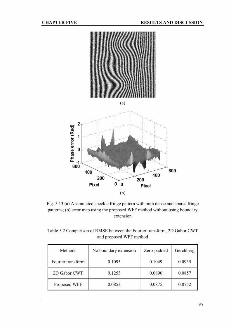
CHAPTER FIVE RESULTS AND DISCUSSION
95
Fig. 5.13 (a) A simulated speckle fringe pattern with both dense and sparse fringe patterns; (b) error map using the proposed WFF method without using boundary
extension
Methods No boundary extension Zero-padded Gerchberg
Fourier transform 0.1095 0.1049 0.0935
2D Gabor CWT 0.1253 0.0890 0.0857
Proposed WFF 0.0853 0.0875 0.0752
Table 5.2 Comparison of RMSE between the Fourier transform, 2D Gabor CWT and proposed WFF method
(b)
(a)

CHAPTER FIVE RESULTS AND DISCUSSION
96
5.2.2 Experimental results
The speckle fringe patterns are obtained from the DSSI with carriers for out-of-plane
displacement derivative measurement. The image size of the speckle fringe pattern
used for processing is 465481 pixels. Figure 5.14(a) shows a speckle fringe pattern
representing the displacement derivative of a deformed flat plate fully clamped at the
boundary and Fig. 5.14(b) shows the carriers introduced. Figure 5.14(c) shows the
extrapolated speckle fringe pattern based on Fig. 5.14(a) by the Gerchberg method.
Figure 5.15(a) shows a phase map retrieved from Fig. 5.14(a) using fast Fourier
transform and Fig. 5.15(b) shows a phase map retrieved from Fig. 5.14(c) using the
proposed WFF method after the removal of excessive extrapolated pixels. Figure
5.15(c) shows a phase map retrieved from Fig. 5.14(a) using the WFF with
convolution method. As can be seen from Fig. 5.15(b), it contains less noise than that
of the fast Fourier transform method shown in Fig. 5.15(a) and is comparable with
that obtained by the WFF with convolution method. The benefit between noise
reduction and signal retention has to be weighed for the WFF method. Figures 5.16(a)
and 5.16(b) show respectively the unwrapped phase maps after carrier removal using
the proposed WFF and the WFF with convolution method. As can be seen, there are
still some noises in the phase map retrieved using the convolution method. This is due
to the difference in the threshold values and the extrapolation method used. Figure
5.16(c) shows a plot of the unwrapped phase values along central line CC in Figs.
5.16(a) and 5.16(b). As can be seen, both methods show similar results with a RMSE
of 0.49 rad. In both methods, the window size is 16, l and h are 0.1 and 0.7

CHAPTER FIVE RESULTS AND DISCUSSION
97
respectively with an interval of 0.1, l and h are -0.3 and 0.3 respectively with an
interval of 0.1. The thresholds used in the proposed WFF and the WFF with
convolution method are 2.55 and 140, respectively. As shown in Table 5.1, the total
computation time using the proposed WFF method for phase retrieved from Fig.
5.14(c) is 44.05 seconds while that by the WFF with convolution method for phase
Fig. 5.14 (a) Speckle fringe pattern indicating displacement derivative; (b) carrier fringe pattern; (c) extrapolated speckle fringe pattern based on (a)
(c)
(a) (b)

CHAPTER FIVE RESULTS AND DISCUSSION
98
retrieval from Fig. 5.14(a) is 337.87 seconds. Here the proposed WFF method has an
advantage in computation time and is not affected by the window size . It is
noteworthy that the boundary effect for phase retrieval is suppressed using the WFF
with convolution method since a zero padded algorithm is employed in the
convolution method.
Fig. 5.15 (a) Retrieved phase map using fast Fourier transform method; (b) retrieved phase map using proposed WFF method; (c) retrieved phase
map using WFF with convolution method
(c)
(a) (b)
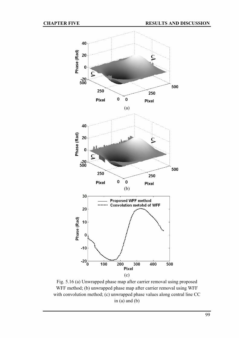
CHAPTER FIVE RESULTS AND DISCUSSION
99
Fig. 5.16 (a) Unwrapped phase map after carrier removal using proposed WFF method; (b) unwrapped phase map after carrier removal using WFF
with convolution method; (c) unwrapped phase values along central line CC in (a) and (b)
C
C
C
C
(a)
(b)
(c)

CHAPTER FIVE RESULTS AND DISCUSSION
100
5.3 Relatively large deformation measurement
In a dense phase fringe pattern, denoising is an important issue in optical
measurement since it determines the measurement range. The ISCAF technique which
uses low-pass filtering is no longer suitable in this case. The WFF technique is
proposed for phase retrieval from noisy and dense phase fringe patterns obtained
using ESPI and DSSI.
5.3.1 Phase fringe denoising in ESPI
For a relatively large deformation measurement in ESPI, phase shifting method has to
be employed and would produce a noisy and dense phase fringe pattern. The Carré
phase shifting algorithm is used in the experiment since it only requires capturing four
phase shifted speckle patterns. To retrieve the correct phase values from a noisy and
dense phase fringe pattern obtained using the Carré phase shifting method, denoising
is required. Numerical simulation work has been carried out to show the effects of the
phase fringe density and speckle size on the results.
5.3.1.1 Simulated results
Figure 5.17 shows a simulated dense wrapped phase map with speckle noise normally
encountered when ESPI is used for large deformation measurement. The simulated
image size of Fig. 5.17 is 513513 pixels which has the same pixel number around
the image center. The wrapped phase map is simulated using five pixels per period
and the phase difference between adjacent pixels in the horizontal direction is / 2

CHAPTER FIVE RESULTS AND DISCUSSION
101
rad. The added noise is Gaussian noise with a zero mean value and a variance of
0.7896. Figure 5.18(a) shows the phase values along the first row of the pixels in Fig.
5.17. As can be seen, the noises introduce errors and difficulties for phase unwrapping
of Fig. 5.17 when filtering is not employed. For speckle noise reduction, the fast WFF
method is employed. Figure 5.18(b) shows a filtered phase fringe pattern using the
fast WFF technique. As can be seen, the noise is effectively suppressed and the
RMSE compared with the theoretical phase values is 0.28 rad. A conventional sine-
cosine average filter using a 3-by-3 window is also used for comparison and the
RMSE is 0.65 rad which is about twice of the fast WFF technique. As can be seen, the
fast WFF technique produces a better result than that of the conventional sine-cosine
Fig. 5.17 Simulated wrapped phase map with speckle noise

CHAPTER FIVE RESULTS AND DISCUSSION
102
average filter. It is noteworthy that when the density of the phase fringe pattern
reduces, the RMSE of the proposed fast WFF technique also reduces. For example,
the RMSE using the proposed technique is 0.07 rad for a phase fringe pattern of 30
Fig. 5.18 (a) Phase values along the first row of pixels in Fig. 5.17; (b) filtered phase fringe pattern using fast WFF technique
(b)
0 100 200 300 400 500-4
-2
0
2
4
Pixel
Phas
e (R
ad)
(a)

CHAPTER FIVE RESULTS AND DISCUSSION
103
pixels per period. It shows that the dense phase fringe pattern is more difficult for
filtering than the sparse phase fringe pattern. In addition, speckle size will also affect
the RMSE using the fast WFF technique. Figure 5.19 shows a plot of speckle size
versus the RMSE. Four sets of noisy phase fringe patterns with different speckle sizes
are simulated and the results are marked as the triangles in the plot. The trend is
shown by a dashed line. As can been seen, with increasing speckle size, the RMSE
using the fast WFF technique increases. This suggests that a smaller speckle size
would produce more accurate results.
5.3.1.2 Experimental results
An ESPI system used is shown in Fig. 4.3. Figure 5.20 shows a phase difference map
retrieved using the Carré phase shifting method. The speckle noise in the phase
difference map will introduce errors in phase unwrapping if filtering is not employed.
Fig. 5.19 A plot of speckle size versus the RMSE
1 1.5 2 2.50.04
0.05
0.06
0.07
0.08
0.09
Speckle size(Pixel)
RM
SE
(Rad
)

CHAPTER FIVE RESULTS AND DISCUSSION
104
Hence the proposed fast WFF technique is employed for denoising. Figure 5.21(a)
shows a filtered phase fringe pattern using the fast WFF technique and Fig. 5.21(b)
shows a filtered phase fringe pattern using the conventional sine-cosine average
filtering technique. Figures 5.22(a) and 5.22(b) show the corresponding unwrapped
phase maps using quality guided phase derivative variance method (Ghiglia and Pritt,
1998). As can been seen, the proposed technique provides a phase fringe pattern with
noise suppressed even in areas with a high fringe density which is suitable for phase
unwrapping to proceed. The unwrapped phase map can further be employed to obtain
the deformation of the object.
Fig. 5.20 Phase difference map retrieved using Carré phase shifting method

CHAPTER FIVE RESULTS AND DISCUSSION
105
Fig. 5.21 (a) Filtered phase fringe pattern by fast WFF technique; (b) filtered phase fringe pattern by conventional sine-cosine average filtering technique
(b)
(a)

CHAPTER FIVE RESULTS AND DISCUSSION
106
5.3.2 Phase fringe denoising in DSSI
Figures 5.23 shows the phase difference maps obtained using a two-wavelength DSSI
system shown in Fig. 4.4. Figures 5.23(a) and 5.23(b) show respectively the phase
difference maps for the red and green lights. Figure 5.24(a) shows a filtered phase
map of Fig. 5.23(a) obtained using the ISCAF technique with a 3 by 3 (smallest
(b)
(a)
Fig. 5.22 (a) Unwrapped phase map by fast WFF technique; (b) unwrapped phase map by conventional sine-cosine average filtering technique

CHAPTER FIVE RESULTS AND DISCUSSION
107
possible) window and with 10 iterations. As can be seen, the phase fringe pattern is
distorted at the central region where the fringe density is high even though the noise at
the region with sparse fringes is filtered. The ISCAF technique is not able to produce
a satisfied result in this case. Figure 5.24(b) shows a phase difference map of the
synthetic wavelength obtained by subtracting the phase difference maps between the
red and green lights without filtering. Figure 5.25(a) shows the filtered phase
difference obtained using the ISCAF (with a 7 by 5 window and 30 iterations) and the
contour of the phase fringes is retrieved. Figure 5.25(b) shows filtered phase values of
Fig. 5.23(a) by the fast WFF technique with filtering parameters 2.1l and
2.1h with a step of 0.2; 0.7l and 0.7h with a step of 0.1; 10 and a
threshold value of 0.07. As can be seen from Fig. 5.25(b), effective filtering is
achieved even in areas of high fringe density. Figures 5.26 and 5.27 show the
Fig. 5.23 (a) Phase difference retrieved for red light; (b) phase difference retrieved for green light
(a) (b)

CHAPTER FIVE RESULTS AND DISCUSSION
108
unwrapped phase maps of Figs. 5.25(a) and 5.25(b), respectively. The phase values of
the synthetic wavelength in Fig. 5.26 is converted to the phase values of the red light
by multiplying a value of /s . Figure 5.28 shows the phase values along cross-
section A-A in Figs 5.26 and 5.27. The dash line is obtained from the converted phase
values of Fig. 5.26 whereas the solid line is from Fig. 5.27. As can been seen, both
techniques produce similar results.
To validate the results, the slope values obtained from cross-section A-A in
Figs 5.26 and 5.27 are compared with those obtained using the strain gauge method.
The strain gauge mounted with two gauges in tension and two gauges in compression
employs a full-bridge circuit. The load at the center point of the fully clamped circular
plate is measured and the displacement derivative for the plate can be estimated from
(a) (b)
Fig. 5.24 (a) Filtered phase of Fig. 5.23(a) obtained with ISCAF; (b) raw phase difference of the synthetic wavelength obtained by subtracting the phase
difference maps between the red and green lights

CHAPTER FIVE RESULTS AND DISCUSSION
109
the measured load. The RMSE between the two-wavelength and the strain gauge
method is 53.95 10 , while the RMSE between the single wavelength and the strain
gauge method is 53.86 10 . As can be seen, the two-wavelength method with ISCAF
shows similar results as the single wavelength method with WFF. However, Fig. 5.28
shows a slight difference in phase values representing the maximum slope. This is due
to an amplification of the error in the two-wavelength method.
It is noteworthy that even though the fast WFF algorithm requires more
manual intervention than the ISCAF technique, it has a good potential for noise
suppression where the fringe density is high. Since the ISCAF technique is a simple
filtering technique with the advantage of less manual intervention, it is employed for
(a) (b)
Fig. 5.25 (a) Filtered phase difference of the synthetic wavelength obtained with ISCAF; (b) filtered phase of Fig. 5.23(a) using fast WFF

CHAPTER FIVE RESULTS AND DISCUSSION
110
noise suppression where the fringe density is relatively low as with two-wavelength
simultaneous illumination.
Fig. 5.27 Unwrapped phase map of Fig. 5.25(b)
A
A
Fig. 5.26 Unwrapped phase map of Fig. 5.25(a)
A
A

CHAPTER FIVE RESULTS AND DISCUSSION
111
5.4 Two-wavelength DSSI using combined filter
The experimental results are obtained for small deformation derivative measurement
in two-wavelength DSSI system shown in Fig. 4.4. Figures 5.29(a) and 5.29(b) show
wrapped phase maps of r (for r 632.8 nm) and g (for g 532 nm)
retrieved by the Carré phase shifting algorithm, respectively. The wrapped phase
maps r and g filtered using the fast WFF technique are shown in Figs. 5.29(c)
and 5.29(d), respectively. Figure 5.30(a) shows a phase map of s for a synthetic
wavelength 3.3398 s µm obtained by subtraction of phase maps shown in Figs.
5.29(c) and 5.29(d) whereas Fig. 5.30(b) shows a filtered phase map s obtained
using the fast WFF technique. The parameters of the fast WFF algorithm used for
obtaining Figs. 5.29(c), 5.29(d) and 5.30(b) are shown in Table 5.3. The phase map
shown in Fig. 5.30(b) is already an unwrapped phase map though no unwrapping
Fig. 5.28 Phase values along cross-section A-A from the unwrapped phase maps using two filtering techniques
Along cross-section A-A of Fig. 5.26
Along cross-section A-A of Fig. 5.27

CHAPTER FIVE RESULTS AND DISCUSSION
112
procedure has been carried out. To improve the sensitivity of the two-wavelength
technique, integral multiples of 2π obtained from s are utilized for unwrapping of
g , the filtered phase map for the green light.
(d) (c)
Fig. 5.29 (a) Wrapped phase r for red light; (b) wrapped phase g for green
light; (c) filtered wrapped phase r ; (d) filtered wrapped phase g
(a) (b)

CHAPTER FIVE RESULTS AND DISCUSSION
113
Table 5.3 Parameters used for the fast WFF algorithm
Window size
Integration in x-direction
: :l step h
Integration in y-direction
: :l step h
Threshold values
Fig. 5.29(c) 10 -1:0.1:1 -0.3:0.1:0.3 0.15
Fig. 5.29(d) 10 -1:0.1:1 -0.3:0.1:0.3 0.15
Fig. 5.30(b) 18 -0.6:0.1:0.6 -0.6:0.1:0.6 0.6
Fig. 5.30 (a) Phase s for synthetic wavelength 3.3398 s µm; (b) filtered
phase s
(a)
(b)

CHAPTER FIVE RESULTS AND DISCUSSION
114
Figure 5.31(a) shows an unwrapped phase map gu obtained using g and
Coef (as explained in Sec. 3.3.2.1) without phase error correction and Fig. 5.31(b)
shows a corresponding 3D plot of the phase values. It can be seen from Fig. 5.31(b)
that there are noticeable errors in the form of spikes which are caused by incorrect 2π
integral multiples obtained from s . gu represents the filtered values of gu and
is assigned the values of gu . Phase error correction algorithm is then applied to
remove the spikes. Figure 5.32(a) shows the phase gu (Line 1) along cross-section
A-A in Fig. 5.31(a) and the corresponding values of _Coef diff (Line 2). Figure
5.32(b) shows the initial distribution of Fig. 5.32(a) from 1 to 120 pixels. As can be
seen, each spike in Line 1 corresponds to a pair of positive and negative numbers in
Line 2. Hence, with the line scanning of the values of _Coef diff , spikes in each line
of gu can be detected and the phase values of gu within the upward and
downward spikes can be corrected by subtracting or adding a value of 2π, respectively.
The corrected phase map gu is shown in Fig. 5.32(c). As can be seen, the spikes
have been removed completely and the derivative of deformation can be evaluated
from gu . The phase values shown in Fig. 5.32(c) have also been compared with the
unwrapped phase obtained by spatially unwrapping g using quality guided phase
derivative variance method and it is found that the RMSE between them is negligible.
Thus the proposed technique using a two-wavelength interferometry has a novelty
that the same level of sensitivity as the single wavelength for phase retrieval is
achieved.

CHAPTER FIVE RESULTS AND DISCUSSION
115
It should be noted that the phase error correction algorithm can be applied
only to continuous surface deformation where the optical path difference between the
adjacent pixels is smaller than the wavelength of the light source used. However, with
the boundary detection algorithm it could be employed for phase retrieval on
discontinuous surface deformation.
Fig. 5.31 (a) Unwrapped phase gu without combined filter;
(b) corresponding 3D plot
A A
(b)
(a)

CHAPTER FIVE RESULTS AND DISCUSSION
116
Fig. 5.32 (a) Phase values (Line 1) and corresponding values of _Coef diff
(Line 2) on cross-section A-A in Fig. 5.31(a); (b) initial values of Fig. 5.32(a)
(from 1 to 120 pixels); (c) phase map gu with combined filter
(c)
(b)
Line 1: Phase values
Line 2: Corresponding values of
_Coef diff Line 1
Line 2
Line 1
Line 2
Line 1: Phase values
Line 2: Corresponding values of _Coef diff
(a)

CHAPTER SIX CONCLUSIONS AND RECOMMENDATIONS
117
CHAPTER SIX
CONCLUSIONS AND RECOMMENDATIONS
6.1 Concluding remarks
In this thesis challenging issues in optical measurement techniques like phase retrieval
and phase unwrapping are discussed in detail. The time-frequency analysis based
techniques for phase retrieval in optical measurement using speckle interferometry
and speckle shearing interferometry are discussed. The 2D Gabor CWT is proposed
for phase retrieval in speckle interferometry with spatial carriers. The advantages of
2D Gabor CWT over 1D wavelet transform in phase retrieval from fringe patterns are
addressed. The proposed 2D Gabor CWT utilized the maximum modulus method to
retrieve phase information from the coefficients of a wavelet transform. The proposed
method is able to reduce the speckle noise effectively. The 2D Gabor wavelet is
employed to demodulate fringe patterns with wide bandwidths which could not be
correctly demodulated by the 2D fan wavelet transform. Simulated and experimental
results show that the proposed 2D Gabor CWT method has a better noise suppression
capability.
A time-frequency analysis based technique, namely the WFT, is also
employed for phase retrieval from speckle fringe patterns. The proposed WFT utilizes
a fast Fourier transform algorithm and reduces computation time significantly
compared with the WFT with convolution method. The proposed WFT method has an

CHAPTER SIX CONCLUSIONS AND RECOMMENDATIONS
118
advantage over the Fourier transform method for phase retrieval since the WFT is a
local transform and simultaneously provides time and frequency information of a
signal, while the Fourier transform is a global transform and the signal in different
region will affect each other so that the noise reduction capability of the Fourier
transform is not satisfied. The proposed WFT method also has an advantage that the
resolution of WFT in both time and frequency domain can be selected according to
the spectrum of a fringe pattern for phase retrieval since a suitable resolution can
retain useful signals and restrict the speckle noise. Simulated and experimental results
have shown the validity of the proposed WFT method.
The WFT method is also employed for noise reduction of dense phase fringe
patterns obtained using the ESPI and DSSI systems. In ESPI, the effect of phase
fringe density and speckle size on the WFF technique is studied and it is shown that a
smaller speckle size would improve the noise suppression capability in the WFF. The
WFF technique is also employed for dense phase fringe denoising using single
wavelength illumination in DSSI for relatively large deformation measurement.
Experimental results show that the WFF technique has a better denoising capability
than the ISCAF technique and is able to extend the measurement range.
Phase retrieval in two-wavelength DSSI using a combined filtering method is
also studied for small deformation derivative measurement. The proposed method
exploits the advantages of a two-wavelength technique and is shown to be an
alternative to phase unwrapping. It also has the potential for measurement of
discontinuous surface profile and deformation when combined with a boundary

CHAPTER SIX CONCLUSIONS AND RECOMMENDATIONS
119
detection algorithm.
In conclusion, the novelties of the proposed 2D Gabor CWT method are that
the proposed 2D Gabor CWT method is able to overcome the narrow spectrum
limitation of the previous 2D CWT and it is also an improvement from the 1D CWT.
The novelties of the improved WFT method are that the improved WFT method has a
significant improvement in reduction of computation time for fringe pattern
demodulation and it is expected in real-time dynamic measurement or for processing a
large amount of fringe patterns. It is a new application to phase retrieval and noise
reduction in DSSI. It is also a suitable method for noise reduction of a dense phase
fringe pattern in relatively large deformation measurement.
6.2 Recommendations
It is recommended that future work could be carried out in the following areas.
Demodulation of a closed fringe pattern is still a challenging problem in
optical measurement. Since the Fourier spectrum of a close fringe pattern overlaps
each other, the phase values of the fringe pattern can not be correctly retrieved. Many
methods have been proposed for phase retrieval on this type of fringe patterns, but
there are still limitations, such as low accuracy and complications. Therefore, suitable
algorithms need to be developed for demodulation of this kind of fringe patterns. One
possible solution is to cut the closed fringe pattern into several regions and perform
phase retrieval for each region before combining them to obtain a final phase map.

CHAPTER SIX CONCLUSIONS AND RECOMMENDATIONS
120
Dynamic interferometry technique can reduce effects of vibration using the
phase shifting interferometry. Since a four-step phase shifting technique was
employed for phase retrieval, the accuracy of phase retrieval may be improved if an
eight-step phase shifting technique is employed. This would require improvement in a
pixelated mask. Thus improvement in phase retrieval technique for the dynamic
interferometry can be further studied.
Fringe projection technique is also widely employed in surface profile
measurement. However, most of the applications are for static measurement. Accurate
color fringe projection using phase shifting method has a potential and can be further
studied for dynamic measurement.

REFERENCES
121
REFERENCES
1. Aebischer, H. A. and S. Waldner, A simple and effective method for filtering speckle-interferometric phase fringe patterns, Opt. Commun. 162, pp. 205-210. 1999.
2. Afifi, M., A. Fassi-Fihri, M. Marjane, K. Nassim, M. Sidki, and S. Rachafi, Paul wavelet-based algorithm for optical phase distribution evaluation, Opt. Commun. 211, pp. 47-51. 2002.
3. Antoine, J. P., P. Carrette, R. Murenzi, and B. Piette, Image analysis with two-dimensional continuous wavelet transform, Signal Processing 31, pp. 241-72. 1993.
4. Bone, D. J., Fourier fringe analysis: the two-dimensional phase unwrapping problem, Appl. Opt. 30, pp. 3627-3632. 1991.
5. Bruck, H. A., S. R. McNeil, M. A. Sutton, and W. H. Peters, Digital image correlation using Newton-Raphson method of partial differential correction, Experimental Mechanics 29, pp. 261-267. 1989.
6. Bruning, J. H., Fringe scanning interferometers, in Optical Shop Testing, D. Malacara, ed. (Wiley, New York), pp. 409-437. 1978.
7. Burke, J., T. Bothe, W. Osten, and C. Hess, Reverse engineering by fringe projection, Proc. SPIE 4778, pp. 312-324. 2002.
8. Carré, P., Installation et utilisation du comparateur photoélectrique et interférentiel du Bureau International des Poids et Mesures, Metrologia 2, pp. 13-23. 1966.
9. Chen, W. J., P. Bu, S. Z. Zheng, and X. Y. Su, Study on Fourier transforms profilometry based on bi-color projecting, Opt. Laser Tech. 39, pp. 821-7. 2007.
10. Cheng, Y. and J. C. Wyant, Two-wavelength phase-shifting interferometry, Appl. Opt. 23, pp. 4539-4543. 1984.
11. Cheng, Y. and J. C. Wyant, Multiple-wavelength phase-shifting interferometry,

REFERENCES
122
Appl. Opt. 24, pp. 804-807. 1985.
12. Choi, Y. B. and S. W. Kim, Phase-shifting grating projection moiré topography, Opt. Eng. 37, pp. 1005-1010. 1998.
13. Chu, T. C., W. E. Ranson, M. A. Sutton, and W. H. Peters, Applications of digital image correlation techniques to experimental mechanics, Experimental Mechanics 25, pp. 232-244. 1985.
14. Creath, K., Phase-shifting speckle interferometry, Appl. Opt. 24, pp. 3053-3058. 1985.
15. Creath, K., Step height measurement using two-wavelength phase-shifting interferometry, Appl. Opt. 26, pp. 2810-2816. 1987.
16. Cuche, E., F. Bevilacqua, and C. Depeursinge, Digital holography for quantitative phase-contrast imaging, Opt. Lett. 24, pp. 291-293. 1999.
17. Dainty, J. C., Laser speckle and related phenomena, in Topics in Applied Physics, vol. 9. Berlin, Germany: Springer-Verlag, 1975.
18. Decker, J. E., J. R. Miles, A. A. Madej, R. F. Siemsen, K. J. Siemsen, S. D. Bonth, K. Bustraan, S. Temple, and J. R. Pekelsky, Increasing the range of unambiguity in step-height measurement with multiple-wavelength interferometry-application to absolute long gauge block measurement, Appl. Opt. 42, pp. 5670-5678. 2003.
19. Dorrío, B. V. and J. L. Fernández, Phase-evaluation methods in whole-field optical measurement techniques, Meas. Sci. Technol. 10, pp. R33-R55. 1999.
20. Durson, A., S. Ozder, and F. N. Ecevit, Continuous wavelet transform analysis of projected fringe patterns, Meas. Sci. Technol. 15, pp. 1768-1772. 2004.
21. Ennos, A. E., Speckle interferometry, in Laser Speckle and Related Phenomena, J. C. Dainty, Ed. (Springer, Berlin), 9, pp. 203-253. 1975.
22. Ettemeyer, A., Combination of 3-D deformation and shape measurement by electronic speckle-pattern interferometry for quantitative strain-stress analysis, Opt. Eng. 39, pp. 212-215. 2000.
23. Fan, H., J. Wang, and Y. S. Tan, Simultaneous measurement of whole in-plane displacement using phase-shifting ESPI, Opt. Laser Eng. 28, pp. 249-57. 1997.
24. Federico, A. and G. H. Kaufmann, Evaluation of the continuous wavelet

REFERENCES
123
transform method for the phase measurement of electronic speckle pattern interferometry fringes, Opt. Eng. 41, pp. 3209-3216. 2002.
25. Flynn, T. J., Consistent 2-D phase unwrapping guided by a quality map, Proceedings of the 1996 International Geoscience and Remote Sensing Symposium. (IGARSS), pp. 057-2059. 1996.
26. Flynn, T. J., Two-dimensional phase unwrapping with minimum weighted discontinuity, J. Opt. Soc. Am. A 14, pp. 2692-2701. 1997.
27. Ford, H. D., H. Atcha, and R.P. Tatam, Optical fibre technique for the measurement of small frequency separations: application to surface profile measurement using electronic speckle pattern interferometry, Meas. Sci. Technol. 4, pp. 601-607. 1993.
28. Funnell, W. R. J., Image processing applied to the interactive analysis interferometric fringes, Appl. Opt. 20, pp. 3245-3250. 1981.
29. Gao, W., N. T. T. Huyen, S. L. Ho, and K. Qian, Real-time 2D parallel windowed Fourier transform for fringe pattern analysis using Graphics Processing Unit, Opt. Express 17, pp. 23147-23152. 2009.
30. Gdeisat, M. A., D. R. Burton, and M. J. Lalor, Spatial carrier fringe pattern demodulation by use of a two-dimensional continuous wavelet transform, Appl. Opt. 45, pp. 8722-32. 2006.
31. Gerchberg, R. W., Super-resolution through error energy reduction, Opt. Acta 21, pp. 709-20. 1974.
32. Ghiglia, D. C., G. A. Mastin, and L. A. Romero, Cellular-automata method for phase unwrapping, J. Opt. Soc. Am. A 4, pp. 267-280. 1987.
33. Ghiglia, D. C. and L. A. Romero, Robust two-dimensional weighted and unweighted phase unwrapping that uses fast transforms and iterative methods, J. Opt. Soc. Am. A 11, pp. 107-117. 1994.
34. Ghiglia, D. C. and L. A. Romero, Minimum Lp-norm two-dimensional phase unwrapping, J. Opt. Soc. Am. A 13, pp. 1999-2013. 1996.
35. Ghiglia, D. C. and M. D. Pritt, Two dimensional phase unwrapping: theory, algorithm and software, New York, Wiley, 1998.
36. Goldstein, R. M., H. A. Zebker, and C. L. Werner, Satellite radar interferometry: two-dimensional phase unwrapping, Radio Sci. 23, pp. 713-

REFERENCES
124
720. 1988.
37. Goodman, J. W., Some fundamental properties of speckle, J. Opt. SOC. Amer. 66, pp. 1145-1149. 1976.
38. Guo, H., H. He, and M. Chen, Gamma correction for digital fringe projection profilometry, Appl. Opt. 43, pp. 2906-2914. 2004.
39. Guo, H., H. He, Y. Yu, and M. Chen, Least-squares calibration method for fringe projection profilometry, Opt. Eng. 44, pp. 033603. 2005.
40. Hack, E., B. Frei, R. Kästle, and U. Sennhauser, Additive-subtractive two-wavelength ESPI contouring by using a synthetic wavelength phase shift, Appl. Opt. 37, pp. 2591-2597. 1998.
41. Huang, J. R., H. D. Ford, and R. P. Tatam, Slope measurement by two-wavelength electronic shearography, Opt. Lasers Eng. 27, pp. 321-333. 1997.
42. Huang, L., Q. Kemao, B. Pan, and A. K. Asundi, Comparison of Fourier transform, windowed Fourier transform, and wavelet transform methods for phase extraction from a single fringe pattern in fringe projection profilometry, Opt. Lasers Eng. 48, pp. 141-148. 2010.
43. Huang, P. S., Q. Hu, F. Jin, and F. P. Chiang, Color-encoded digital fringe projection technique for high-speed three dimensional surface contouring, Opt. Eng. 38, pp. 1065-1071. 1999.
44. Huang, P. S., C. Zhang, and F. P. Chiang, High-speed 3-D shape measurement based on digital fringe projection, Opt. Eng. 42, pp. 163-168. 2003.
45. Huang, P. S. and S. Zhang, Fast three-step phase-shifting algorithm, Appl. Opt. 45, pp. 5086-5091. 2006.
46. Hung, Y. Y. and C. E. Taylor, Speckle-shearing interferometric camera-a tool for measurement of derivatives of surface-displacement, In: SPIE Proc. 41, pp. 169-175. 1973.
47. Hung, Y. Y. and A. J. Durelli, Simultaneous measurement of three displacement-derivatives using a multiple image shearing interferometric camera, J. Strain Anal. 14, pp. 81-88. 1979.
48. Hung, Y. Y., Shearography: a new optical method for strain measurement and nondestructive testing, Opt. Eng. 21, pp. 391-395. 1982.

REFERENCES
125
49. Hung, Y. Y., Computerized shearography and its application for nondestructive evaluation of composites, in Manual on Experimental Methods of Mechanical Testing of Composites, C. H. Jenkins, Ed., Society for Experimental Mechanics, Bethel, CT, 1998.
50. Huntley, J. M. and H. O. Saldner, Temporal phase unwrapping algorithm for automated interferogram analysis, Appl. Opt. 32, pp. 3047-3052. 1993.
51. Huntley, J. M. and H. O. Saldner, Shape measurement by temporal phase unwrapping: comparison of unwrapping algorithm, Meas. Sci. Technol. 8, pp. 986-992. 1997a.
52. Huntley, J. M. and H. O. Saldner, Error reduction methods for shape measurement by temporal phase unwrapping, J. Opt. Soc. Am. A 14, pp. 3188-3196. 1997b.
53. Høgmoen, K. and O. J. Løkberg, Detection and measurement of small vibrations using electronic speckle pattern interferometry, Appl. Opt. 16, pp. 1869-1875. 1977.
54. Iwahashi, Y., K. Iwata, and R. Nagata, Influence of in-plane displacement in single-aperture and double-aperture speckle shearing interferometry, Appl. Opt. 24, pp. 2189-2192. 1985.
55. Jin, L., T. Yoshizawa, and Y. Otani, Shadow moiré profilometry using the phase-shifting method, Opt. Eng. 39, pp. 2119-2123. 2000.
56. Jin, L. H., Y. Otani, and T. Yoshizawa, Shadow moiré profilometry by frequency sweeping, Opt. Eng. 40, pp. 1383-1386. 2001.
57. Joenathan, C. and B. M. Khorana, Phase-measuring fiber optic electronic speckle pattern interferometer: phase step calibration and phase drift minimization, Opt. Eng. 31, pp. 315-321. 1992.
58. Johansson, S. and K. G. Predko, Performance of a phase-shifting speckle interferometer for measuring deformation and vibration, J. Phys. E Sci. Instrum. 22, pp. 289-292. 1989.
59. Judge, T. R. and P. J. Bryanston-Cross, A review of phase unwrapping techniques in fringe analysis, Opt. Lasers Eng. 21, pp. 199-239. 1994.
60. Kadooka, K., K. Kunoo, N. Uda, K. Ono, and T. Nagayasu, Strain analysis for moiré interferometry using the two-dimensional continuous wavelet transform, Exp. Mech. 43, pp. 45-51. 2003.

REFERENCES
126
61. Kato, J., I. Yamaguchi, and Q. Ping, Automatic deformation analysis by a TV speckle interferometer using a laser diode, Appl. Opt. 32, pp. 77-83. 1993.
62. Kaufmann, G. H. and G. E. Galizzi, Phase measurement in temporal speckle pattern interferometry: comparison between the phase-shifting and the Fourier transform methods, Appl. Opt. 41, pp. 7254-63. 2002.
63. Kaufmann, G. H., Phase measurement in temporal speckle pattern interferometry using the Fourier transform method with and without a temporal carrier, Opt. Comm. 217, pp. 141-9. 2003.
64. Kirby, F., Which wavelet best reproduces the Fourier power spectrum, Comput. Geosci. 31, pp. 846-64. 2005.
65. Kong, I. B. and S. W. Kim, General algorithm of phase-shifting interferometry by iterative least-squares fitting, Opt. Eng. 34, pp. 183-187. 1995.
66. Kreis, T., Handbook of holographic interferometry, Wiley-VCH, 2005.
67. Kumar, U. P., N. K. Mohan, and M. P. Kothiyal, Measurement of discontinuous surfaces using multiple-wavelength interferometry, Opt. Eng. 48, pp. 073603. 2009a.
68. Kumar, U. P., B. Bhaduri, N. K. Mohan, and M. P. Kothiyal, Two wavelength micro-interferometry for 3-D surface profiling, Opt. Lasers Eng. 47, pp. 223-229. 2009b.
69. Kumar, U. P., N. K. Mohan, M. P. Kothiyal, and A. K. Asundi, Deformation and shape measurement using multiple wavelength microscopic TV holography, Opt. Eng. 48, pp. 023601. 2009c.
70. Lim, H., W. Xu, and X. Huang, Two new practical methods for phase unwrapping, IEEE Trans. Geosci. Remote Sens. IGARSS’95 33, Firenze, Italy, pp. 196-198. 1995.
71. Løkberg, O. J. and K. Høgmoen, Vibration phase mapping using electronic speckle pattern interferometry, Appl. Opt. 15, pp. 2701-2704. 1976.
72. Løkberg, O. J. and J. T. Malmo, Detection of defects in composite materials by TV-holography, NDT Int. 21, pp. 223-228. 1988.
73. Lu, Y., X. Wang, and X. Zhang, Weighted least-squares phase unwrapping algorithm based on derivative variance correlation map, Optik 118, pp. 62-66. 2007.

REFERENCES
127
74. Macy, W. W, Two-dimensional fringe-pattern analysis, Appl. Opt. 22, pp. 3898-3901. 1983.
75. Malacara, D., M. Servin, and Z. Malacara, Interferogram analysis for optical testing, Marcel Dekker, New York, 1998.
76. Mallat, S., A wavelet tour of signal processing. 2nd ed. San Diego: Academic Press. 2001.
77. Massie, N. A., R. D. Nelson, and S. Holly, High-performance real-time heterodyne interferometry, Appl. Opt. 18, pp. 1797-1803. 1979.
78. Meadows, D. M., W. O. Johnson, and J. B. Allen, Generation of surface contours by moiré patterns, Appl. Opt. 9, pp. 942-947. 1970.
79. Mohan, N. K. and R.S. Sirohi, Fringe formation in multiaperture speckle shear interferometry, Appl. Opt. 35, pp. 1617-1622. 1996.
80. Moore, A. J. and J. R. Tyrer, An electronic speckle pattern interferometer for complete in-plane displacement measurement, Meas. Sci. Technol. 1, pp. 1024-1030. 1990.
81. Nakadate, S., T. Yatagai, and H. Saito, Digital speckle-pattern shearing interferometry, Appl. Opt. 19, pp. 4241-4246. 1980.
82. Patil, A. and P. Rastogi, Moving ahead with phase, Opt. Lasers Eng. 45, pp. 253-257. 2007.
83. Pedrini, G., Y. L. Zou, and H. Tiziani, Quantitative evaluation of digital shearing interferogram using the spatial carrier method, Pure Appl. Opt. 5, pp. 313-321. 1996.
84. Polhemus, C., Two-wavelength interferometry, Appl. Opt. 12, pp. 2071-2074. 1973.
85. Qian, K., Windowed Fourier transform for fringe pattern analysis, Appl. Opt. 43, pp. 2695-2702. 2004.
86. Qian, K., On window size selection in the windowed Fourier ridges algorithm, Opt. Lasers Eng. 45, pp. 1186-1192. 2007a.
87. Qian, K., Two-dimensional windowed Fourier transform for fringe pattern analysis: principles, applications and implementations, Opt. Lasers Eng. 45, pp. 304-317. 2007b.

REFERENCES
128
88. Quiroga, J. A., A. Gonzalez-Cano, and E. Bernabeu, Phase unwrapping algorithm based on an adaptive criterion, Appl. Opt. 34, pp. 2560-2563. 1995.
89. Rastogi, P. K., Digital speckle pattern interferometry and related techniques, West Sussex: Wiley, 2001.
90. Robinson, D. W. and G. T. Reid, Interferogram analysis: Digital fringe pattern measurement techniques, Institute of Physics, Bristol, UK, 1993.
91. Roddier, C. and F. Roddier, Interferogram analysis using Fourier transform techniques, Appl. Opt. 26, pp. 1668-73. 1987.
92. Saldner, H. O. and J. M. Huntley, Profilometry by temporal phase unwrapping and spatial light modulator based fringe projector, Opt. Eng. 36, pp. 610-615. 1997a.
93. Saldner, H. O. and J. M. Huntley, Temporal phase unwrapping: application to surface profiling of discontinuous objects, Appl. Opt. 36, pp. 2770-2775. 1997b.
94. Sandoz, P., Wavelet transform as a processing tool in white light interferometry, Opt. Lett. 22, pp. 1065-1067. 1997.
95. Shang, H. M., Y. Y. Hung, W. D. Luo, and Frank Chen, Surface profiling using shearography, Opt. Eng. 39, pp. 23-31. 2000a.
96. Shang, H. M., C. G. Quan, C. J. Tay, and Y. Y. Hung, Generation of carrier fringes in holography and shearography, Appl. Opt. 39, pp. 2638-2645. 2000b.
97. Slettemoen, G. A., Electronic speckle pattern interferometric system based on a speckle reference beam, Appl. Opt. 19, pp. 616-623. 1980.
98. Su, X. and W. Chen, Fourier transform profilometry: a review, Opt. Lasers Eng. 35, pp. 263-84. 2001.
99. Takasaki, H., Moiré topography, Appl. Opt. 9, pp. 1467-1472. 1970.
100. Takasaki, H., Moiré topography, Appl. Opt. 12, pp. 845-850. 1973.
101. Takeda, M., H. Ina, and S. Kobayashi, Fourier-transform method of fringe-pattern analysis for computer-based topography and interferometry, J. Opt. Soc. Am. 72, pp. 156-160. 1982.
102. Takeda, M. and K. Mutoh, Fourier transform profilometry for the automatic

REFERENCES
129
measurement of 3-D object shapes, Appl. Opt. 22, pp. 3977-3982. 1983.
103. Trillo, C., A. F. Doval, D. Cernadas, O. López, J. C. López, B. V. Dorrío, J. L. Fernández, and M. Pérez-Amor, Measurement of the complex amplitude of transient surface acoustic waves using double-pulsed TV holography and a two-stage spatial Fourier transform method, Meas. Sci. Technol. 14, pp. 2127-34. 2003.
104. Vest, C. M., Holographic interferometry, Wiley, New York, 1979.
105. Wagner, C., W. Osten, and S. Seebacher, Direct shape measurement by digital wavefront reconstruction and multiwavelength contouring, Opt. Eng. 39, pp. 79-85. 2000.
106. Wang, D. N., Y. N. Ning, K. T. V. Grattan, A. W. Palmer, and K. Weir, Three-wavelength combination source for white-light interferometry, IEEE Photon. Technol. Lett. 5, pp. 1350-1352. 1993.
107. Wang, J. and A. Asundi, Strain contouring with Gabor filters: filter bank design, Appl. Opt. 41, pp. 7229-36. 2002.
108. Wang, W., C. Hwang, and S. Lin, Vibration measurement by the time-averaged electronic speckle pattern interferometry methods, Appl. Opt. 35, pp. 4502-4509. 1996.
109. Wang, Z. and H. Ma, Advanced continuous wavelet transform algorithm for digital interferogram analysis and processing, Opt. Eng. 45, pp. 045601. 2006.
110. Warnasooriya, N. and M. K. Kim, Quantitative phase imaging using three-wavelength optical phase unwrapping, J. Mod. Opt. 56, pp. 67-74. 2009.
111. Watkins, L. R., S. M. Tan, and T. H. Barnes, Interferometer profile extraction using continuous wavelet transform, Electronics Letters 33, pp. 2116-2117. 1997.
112. Watkins, L. R., S. M. Tan, and T. H. Barnes, Determination of interferometer phase distributions by use of wavelets, Opt. Lett. 24, pp. 905-907. 1999.
113. Watkins, L. R., Phase recovery from fringe patterns using the continuous wavelet transform, Opt. Lasers Eng. 45, pp. 298-303. 2007.
114. Wyant, J. C., Testing aspherics using two-wavelength holography, Appl. Opt. 10, pp. 2113-2118. 1971.
REFERENCES
130
115. Wyant, J. C., Dynamic interferometry, Opt. Phot. News 14, pp. 38-41. 2003.
116. Xiao, F., J. Wu, L. Zhang, and X. Li, A new method about placement of the branch cut in two-dimensional phase unwrapping, IEEE trans. 1-4244-1188-2, 2007.
117. Xu, W. and I. Cumming, A region-growing algorithm for In-SAR phase unwrapping, IEEE Trans. Geosci. Remote Sens. IGARSS’96 34, Lincoln, Nebraska, USA, pp. 2044-2046. 1996.
118. Yamaguchi, I. and T. Zhang, Phase-shifting digital holography, Opt. Lett. 22, pp. 1268-1270. 1997.
119. Yamaguchi, I., Digital holography and three-dimensional display, pp. 145-171. 2006.
120. Yet Another Wavelet Toolbox (YAWTB), home page: http://rhea.tele.ucl.ac.be/yawtb/.
121. Yokozeki, S., K. Patorski, and K. Ohnishi, Collimation method using Fourier imaging and moiré techniques, Opt. Commun. 14, pp.401-405. 1975.
122. Zhang, S. and S. T. Yau, Generic nonsinusoidal phase error correction for three-dimensional shape measurement using a digital video projector, Appl. Opt. 46, pp. 36-43. 2007.
123. Zheng, S. Z., W. J. Chen, and X. Y. Su, Adaptive windowed Fourier transform in 3-D shape measurement, Opt. Eng. 45, pp. 63601-1-4. 2006.
124. Zhong, J. G. and H. P. Zeng, Multiscale windowed Fourier transform for phase extraction of fringe patterns, Appl. Opt. 46, pp. 2670-2675. 2007.
125. Zhong, J. and J. Weng, Spatial carrier-fringe pattern analysis by means of wavelet transform: wavelet transform profilometry, Appl. Opt. 43, pp. 4993-4998. 2004a.
126. Zhong, J. and J. Weng, Dilating Gabor transform for the fringe analysis of 3-D shape measurement, Opt. Eng. 43, pp. 895-899. 2004b.
127. Zhong, J. and J. Weng, Phase retrieval of optical fringe patterns from the ridge of a wavelet transform, Opt. Lett. 30, pp. 2560-2562. 2005.

APPENDICES
131
APPENDICES
Appendix A. Code for 2D Gabor and 2D fan CWT
This program is for 2D Gabor and 2D fan CWT in fringe demodulation using Matlab
software. The algorithm is programmed with the aid of the Yet Another Wavelet
Toolbox (YAWTB).
function [cwtcoef scalex anglex] = cwt2d(fimg, waveletname, scales, angles)
% Two-dimensional continuous wavelet transform for phase retrieval from fringe
patterns with carriers
% fimg: Fourier transform of the fringe pattern
% waveletname: Name of the wavelet to use
% scales, angles : Scales and angles of the wavelet transform to use
% cwtcoef : Coefficients of the wavelet transform by maximum modulus method
% scalex, anglex : Scales and angles obtained by maximum modulus method
% The algorithm of 2D wavelet transform is composed with the aid of YAW Toolbox
(Yet Another Wavelet Toolbox)
% YAW Toolbox : http://rhea.tele.ucl.ac.be/yawtb/
% Obtain the wavelet name
waveletname = lower([waveletname '2d']);
% Obtain the image size

APPENDICES
132
[Hgth,Wdth] = size(fimg);
% Warning if the scales contain nonpositive numbers
for i = 1:length(scales)
if (scales(i) <= 0)
error('''scales'' must be positive');
end
end
% Construct x and y coordinates in Fourier spectrum
num_half = floor((Wdth-1)/2);
freqlx = 2*pi/Wdth*[ 0:num_half (num_half-Wdth+1):-1 ];
num_half = floor((Hgth-1)/2);
freqly = 2*pi/Hgth*[ 0:num_half (num_half-Hgth+1):-1 ];
[fx,fy] = meshgrid(freqlx,freqly);
% Obtain the number of scales and angles
nsc = length(scales);
nang = length(angles);
h = waitbar(0,'Please wait...'); % Create the progress bar
% Define the parameters for the wavelet transform
cwtcoef = fimg; cwtcoef = 0; scalex = cwtcoef; anglex = cwtcoef;
% Wavelet transform of the maximum modulus method
for scnum = 1:nsc,
for angnum = 1:nang,

APPENDICES
133
sc = scales(scnum); % Take a scale from the scale vector
ang = angles(angnum); % Take an angle from the angle vector
% Perform the dilation and rotation of the wavelet in the frequency domain
nfx = sc * ( cos(ang).*fx - sin(ang).*fy );
nfy = sc * ( sin(ang).*fx + cos(ang).*fy );
% Generate a wavelet function in the frequency domain
wavf = sc * feval(waveletname,nfx,nfy);
% Perform wavelet transform
out = ifft2(fimg.* conj(wavf));
% Obtain coefficients of the wavelet transform with maximum modulus method
coef = abs(out)>abs(cwtcoef);
cwtcoef = coef.*out+~coef.*cwtcoef;
scalex = coef*sc+~coef.*scalex; % Obtain scale parameters of the wavelet
transform with maximum modulus method
anglex = coef*ang+~coef.*anglex; % Obtain angle parameters of the wavelet
transform with maximum modulus method
waitbar(scnum/nsc) % Display of the progress bar
end
end

APPENDICES
134
function [out] = morlet2d(kx,ky)
% Generate a 2D Gabor wavelet using 2D Morlet wavelet function
% kx, ky : x and y coordinates in the frequency domain
% out : Output of the 2D Gabor wavelet in the frequency domain
% Define wavelet parameters
k_0 = 5.336;
sigma = 1/2; % Resolution control
% Fourier spectrum of the wavelet function
out = exp( - sigma^2 * ((kx - k_0).^2 + ky.^2)/2 );
function [out] = fan2d(kx,ky)
% 2D fan wavelet
% kx, ky : x and y coordinates in the frequency domain
% out : Output of the 2D fan wavelet in the frequency domain
% Define wavelet parameters
k_0 = 5.336;
sigma = 1/2; % Resolution control
% Superposition of 6 Morlet wavelets
out = 0;
for count = 1:6
sita = (count-1)*pi/6;
% Fourier spectrum of the wavelet function

APPENDICES
135
outtemp = exp( - sigma^2 * ((ky - k_0*cos(sita)).^2 + (kx- k_0*sin(sita)).^2)/2 );
out = out+outtemp;
end
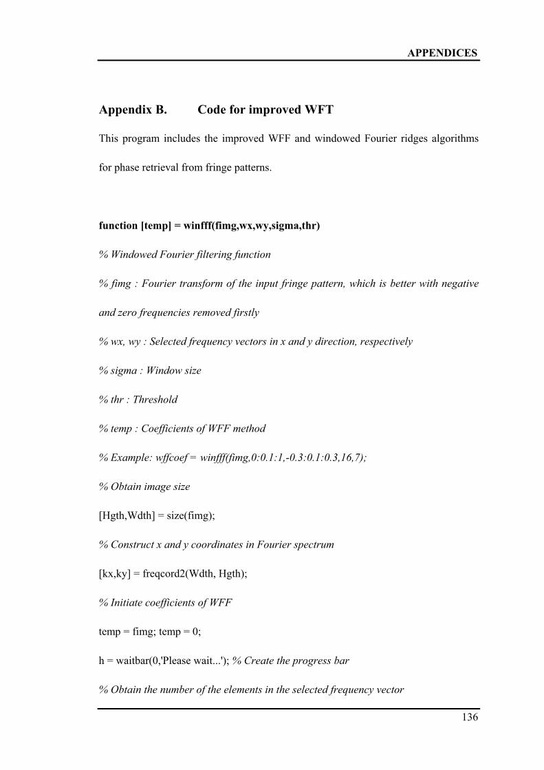
APPENDICES
136
Appendix B. Code for improved WFT
This program includes the improved WFF and windowed Fourier ridges algorithms
for phase retrieval from fringe patterns.
function [temp] = winfff(fimg,wx,wy,sigma,thr)
% Windowed Fourier filtering function
% fimg : Fourier transform of the input fringe pattern, which is better with negative
and zero frequencies removed firstly
% wx, wy : Selected frequency vectors in x and y direction, respectively
% sigma : Window size
% thr : Threshold
% temp : Coefficients of WFF method
% Example: wffcoef = winfff(fimg,0:0.1:1,-0.3:0.1:0.3,16,7);
% Obtain image size
[Hgth,Wdth] = size(fimg);
% Construct x and y coordinates in Fourier spectrum
[kx,ky] = freqcord2(Wdth, Hgth);
% Initiate coefficients of WFF
temp = fimg; temp = 0;
h = waitbar(0,'Please wait...'); % Create the progress bar
% Obtain the number of the elements in the selected frequency vector

APPENDICES
137
nwx = length(wx);
nwy = length(wy);
% Compute the WFF coefficients by fast Fourier transform
for cx = 1:nwx
for cy = 1:nwy
% Take an element from the selected frequency vector
wx1 = wx(cx);
wy1 = wy(cy);
% Compute windowed Fourier basis in frequency domain
mask = win(kx,ky,wx1,wy1,sigma);
% Perform WFT
out = ifft2(fimg.*mask);
% Filter the coefficients of the transform by a threshold
out = out.*(abs(out)>=thr);
% Perform inverse WFT
out = fft2(out);
temp = temp+ifft2(out.*mask);
end
waitbar(cx/nwx) % Display of the progress bar
end

APPENDICES
138
function [temp scalex scaley] = winffr(fimg,wx,wy,sigma)
% Windowed Fourier ridges method
% fimg : Fourier transform of the input fringe pattern, which is better with negative
and zero frequencies removed firstly
% wx, wy : Selected frequency vectors in x and y direction, respectively
% sigma : Window size
% temp : Coefficients of windowed Fourier ridges method
% scalex, scaley : Obtained frequency parameters in x and y direction of the
transform with the maximum modulus method
% Example : wfrcoef = winffr(fimg,0:0.1:1,-0.3:0.1:0.3,12);
% Obtain image size
[Hgth,Wdth] = size(fimg);
% Construct x and y coordinates in the Fourier spectrum
[kx,ky] = freqcord2(Wdth, Hgth);
% Initiate coefficients of windowed Fourier ridges method
temp = fimg; temp = 0; scalex = temp; scaley = temp;
h = waitbar(0,'Please wait...'); % Create the progress bar
% Obtain the number of the elements in the selected frequency vector
nwx = length(wx);
nwy = length(wy);
% Compute coefficients of windowed Fourier ridges method by fast Fourier transform
for cx = 1:nwx

APPENDICES
139
for cy = 1:nwy
% Take an element from the selected frequency vector
wx1 = wx(cx);
wy1 = wy(cy);
% Compute the windowed Fourier basis in the frequency domain
mask = win(kx,ky,wx1,wy1,sigma);
% Perform WFT
out = ifft2(fimg.* conj(mask));
% Peroform the maximum modulus mehtod
coef = abs(out)>abs(temp);
% Obtain the coefficients of the transform with the maximum modulus
temp = coef.*out+~coef.*temp;
% Obtain the frequency parameters of the transform with the maximum modulus
scalex = coef*wx1+~coef.*scalex;
scaley = coef*wy1+~coef.*scaley;
end
waitbar(cx/nwx) % Display of the progress bar
end

APPENDICES
140
function [freqx,freqy] = freqcord2(Wdthx, Hgthy)
% Construct x and y coordinates in the Fourier spectrum
% freqx, freqy : Matrixs of x and y coordinates of the Fourier spectrum
% Wdthx, Hgthy : Width and height of the image
[freqx,freqy] = meshgrid(freqcord1(Wdthx),freqcord1(Hgthy));
function dout = freqcord1(vars)
% Construct the coordinates in the Fourier spectrum
vars_2 = floor((vars-1)/2);
dout = 2*pi/vars*[ 0:vars_2 (vars_2-vars+1):-1 ];
function [out] = win(kx,ky,wx,wy,sigma)
% Compute window function in frequency domain
out = exp( - sigma^2 * ((kx - wx).^2 + (ky-wy).^2)/2 );

APPENDICES
141
Appendix C. List of publications
Journal papers:
1. H. Niu, C. Quan, and C.J. Tay, “Phase retrieval of speckle fringe pattern with
carriers using 2D wavelet transform”, Opt. Lasers Eng. 47(12), 1334-1339, (2009).
2. C. Quan, H. Niu, and C.J. Tay, “An improved windowed Fourier transform for
fringe demodulation”, Opt. Laser Technol. 42(1), 126-131, (2010). 3. H. Niu, C. Quan, C.J. Tay, and B. Bhaduri, “Phase retrieval in DSSI for relatively
large deformation”, Opt. Commun. 284(1), 118-122, (2011). 4. Basanta Bhaduri, C.J. Tay, C. Quan, H. Niu, and Mikael Sjödahl, “Two
wavelength simultaneous DSPI and DSP for 3D displacement field measurements”, Opt. Commun. 284, 2437-2440, (2011).
5. C.J. Tay, C. Quan, H. Niu, and B. Bhaduri, “Phase retrieval in two-wavelength
DSSI using a combined filtering method”, Optik 122(23), 2114-2118, (2011).
Conference papers:
6. H.T. Niu, C. Quan, and C.J. Tay, “Temporal Paul wavelet analysis for phase
retrieval using shadow moiré technique”, Proc. SPIE 7155, 71552B (2008). 7. H. Niu, C. Quan, and C.J. Tay, “A modified WFT for shape and deformation
measurement”, Proc. SPIE 7522, 752247 (2009). 8. H. Niu, C. Quan, and C.J. Tay, “Phase retrieval in ESPI from a dense phase
fringe pattern”, Proc. SPIE 7718, 771817 (2010).