DEVELOPMENT OF MILES-IN-TRAIL PASSBACK RESTRICTIONS FOR AIR TRAFFIC MANAGEMENT

Kapil Sheth, NASA Ames Research Center, Moffett Field, CA Sebastian Gutierrez-Nolasco, UC Santa Cruz, Moffett Field, CA

Abstract

This paper presents modeling of miles-in-trail passback restrictions for use in air traffic management. Generally, FAA managers employ miles-in-trail as a traffic management initiative when downstream traffic congestion at airports or in sectors is anticipated. In order to successfully implement the miles-in-trail at airspace fixes or navigational aids, it is desired that restriction values be computed for passing back to upstream facilities at specific boundaries. This paper presents a model which can be used for that purpose. This model improves on a previous version using traffic manager feedback resulting in significant improvement in guidance. The modeling approach is described along with lessons learned and improvements made during model development. Results for two sample traffic and one real traffic scenarios are presented. Additional operational considerations required by the traffic managers to implement the passback restrictions, namely maximum ground delay and absorbable airborne delay are incorporated in the model. A main result of this research is that absorbing small amount of ground and airborne delays are sufficient to handle the imposed constraint. Another finding is that implementing the passback restrictions provides the traffic managers ways to alleviate traffic constraints to help reduce excessive airborne delay for current traffic conditions.

Introduction The air traffic managers of the National

Airspace System (NAS) in the United States regularly implement various Traffic Management Initiatives (TMIs) to handle traffic in a safe and efficient manner. One such initiative is the Miles-in-Trail (MIT) restriction. Imposed MIT is the value of spacing required between aircraft flying along a certain flight path. They help air traffic managers control the flow of aircraft downstream of an air traffic control facility. MITs could be implemented independently or in conjunction with other TMIs,

e.g., a severe weather avoidance plan route (also referred to as a Playbook route). If a certain facility is unable to manage traffic with the imposed MIT value, it passes back restrictions to one or more upstream facilities. It is important to model these restrictions in a NAS-based simulation environment in order to predict the impact on flight delays, of imposing a certain value of MIT value along a particular path, and perhaps additional passback values.

Some research articles are available which document the modeling of the Miles-in-Trail restrictions. Sridhar [1] presented an integrated set of traffic management initiatives implemented within the Future ATM (Air Traffic Management) Concepts Evaluation Tool (FACET) [2]. Wanke [3] presented an integrated impact assessment capability. Both of those studies were more than a decade ago. Since then, the traffic patterns have changed and other new traffic management initiatives have been developed (e.g., Airspace Flow Programs, Collaborative Trajectory Options Program). Grabbe [4] presented modeling and evaluation of MIT restrictions in the NAS. A linear programming model was developed for implementing MITs for departure flows out of New York area airports. Kopardekar [5] presented a perspective on the MIT operations. The strengths and weaknesses associated with the MIT modeling were presented in that paper, along with the Minutes-in-Trail (MinIT) concept. A refined modeling of the initial work presented by Wanke et al. was presented in two subsequent works. They are by Ostwald [6] on the MIT impact assessment capability, and by DeArmon [7] on the validation of the MIT model. The reported MIT model appears to be a robust capability but some of the implementation issues (e.g., the range limit, multiple stream analysis, passback of restrictions, etc.) are not directly applicable or missing for current operations and traffic. Not many simulation environments are available which model these initiatives across the country in the en route environment. The fidelity of the MIT models is limited and not all aspects of a

Miles-in-Trail restriction are available, especially operationally viable recommendation of passback values to upstream traffic management facilities.

In the earlier paper, Sheth et al. [8] presented a model for computing MIT and passback restrictions in the NAS for current traffic conditions. The focus of this paper is in extending the model presented there with additional capabilities and traffic manager feedback. Two parameters needed for traffic management, namely maximum ground delay for pre-departure flights and absorbable airborne delay between boundaries are added to the model. Results are presented for the CAN_1_East Playbook route for three scenarios. This research is conducted to aid current operations but the model is interoperable for time-based metering, where the future of air traffic management lies.

The rest of the paper is as follows. First the simulation environment used for this research is described. Then, the modeling approach is presented along with improvements from previous models. The

results are presented next. Plans for future work and conclusions are at the end of the paper.

Simulation Environment The FACET software developed at NASA Ames

Research Center was used for this study. FACET is a modeling and analysis system developed to explore advanced ATM concepts. The simulation mode in FACET allows a user to take initial traffic conditions from a certain time and evolves the air traffic based on data provided by the FAA’s Traffic Flow Management System (TFMS) [9] consisting of flight plans that provide origin, destination, route of flight, aircraft type, cruise speed, cruise altitude and takeoff time. The flight plan intent is used for assessing which flights would be impacted by the Playbook routes and associated MIT restrictions. Figure 1 shows a snapshot of FACET graphical user interface. Three FAA published and most used [8] Playbook routes during 2010-2012, CAN_1_East, VUZ, and FL2NE1, are shown. They are shown in green, along with some of

Figure 1. Snapshot of FACET showing three Playbook routes and associated fixes.

the fixes associated with the CAN_1_East route, e.g., Aberdeen, SD (ABR) in Minneapolis Center (ZMP) and Rapid City, SD (RAP), Meeker, CO (EKR), Crazy Woman, WY (CZI) all three in Denver Center (ZDV), and Helena, MT (HLN) in Salt Lake Center (ZLC). Similarly, Vulcan, AL (VUZ), Little Rock, AK (LIT) and Sidon, MS (SQS) are shown along the VUZ route, while Raleigh Durham, NC (RDU), Charlotte, NC (CLT), and CAMRN, NY are seen along the Florida to Northeast (FL2NE1) route. The 20 Center boundaries are shown in gray and the state boundaries are shown in red. Using the simulation capabilities of FACET, aircraft were flown along the CAN_1_East route (shown in Fig. 2) along with the imposed MIT values. These are described in Modeling Approach and Results Sections next.

Modeling Approach The model presented in this paper extends the

research presented in [8]. The new model can handle multiple merging streams of traffic

simultaneously, MIT values at multiple locations across those traffic streams, and optional passback to an upstream Center, along with imposition of maximum ground delay and absorbable airborne delay for flights. In this Section, first the parameters needed for the model are specified, along with model improvements compared to previous research. The scheduling of aircraft and computation of passback restriction values is presented next. The computation engine employing FACET’s predictive capability for the Rapid Evaluation Mode (REM), which uses the scheduling process, is described last.

Parameter Specification A description of the parameters required for

the modeling is presented here. Fig. 2 is a representation of a case where the traffic streams are shown by green lines and the affected aircraft by yellow triangles at 22:45 UTC on Aug. 21, 2012, a similar traffic day. There are two streams merging at ABR, one from ZDV (RAP) and the other from

Figure 2. Implementation of CAN_1_East Playbook route with associated metering boundaries for

passback restrictions and airspace fixes.

B1

B4

B3

B2

B2IN

B4IN

ZLC (HLN). Normally, the stream coming from ZDV has more aircraft than the one coming from ZLC. In order to prevent sector congestion and other traffic flow management issues near ABR, boundary crossing locations, represented by thick light green bars (see Fig. 2), are used to calculate MIT values that can be passed back to upstream facilities. An FAA published restriction from July 3, 2012 for CAN_1_East Playbook route contained the following: “CAN1, 15:45-03:00 UTC, ABR, 40MIT, ZMP, ZDV, JETS, Reason: Vol Enrt Sctr”. This indicates that Minneapolis Center (ZMP) requested Denver Center (ZDV) 40 MIT for ABR fix for jets flying east from 15:45 to 03:00 (next day) UTC. To mitigate this constraint, Minneapolis Center (ZMP) would request an MIT from Denver Center (ZDV), along the RAP boundary (B1), and Salt Lake Center (ZLC), along the HLN path (B2). Typically, these passback values are requested based on what was previously used. Using these parameters, it is desired that the model compute the upstream passback restrictions from ZMP to ZLC and ZDV, and in turn, ZDV to ZLC, along the CZI (B3) and EKR (B4) boundaries for the requested start and end times. It should be noted that the passed back restrictions may not be needed for the same times as the primary restriction start and end times at ABR.

In this MIT model, a metering constraint is modeled as an ordered list. It contains the name of the restriction, metered location, metered direction, start time, end time, and an optional list of crossing boundary locations, which are modeled as a metering constraint and used by the REM. The REM is employed to quickly evaluate and recommend passback values for upstream Centers. The metering constraint is considered active during the time interval specified by the start and end times. Since the recorded data used for this study do not provide information whether the aircraft were jets or propeller-driven, this model does not distinguish them. This could be a significant limitation and will be addressed in future.

An aircraft is considered subject to metering, if it is predicted to pass through the metered location in the specified metered direction when the metering constraint is active. For example, aircraft within ZMP boundary (between ABR and B1) are metered on a first-come, first-served basis by the

aircraft scheduler (described below). The first aircraft is scheduled as is, since there are no other aircraft ahead of it, while subsequent aircraft are to be delayed. The subsequent aircraft may be delayed (by vectoring or in a holding pattern), depending on its performance capability for speed reduction.

Model Improvements In the previous model, each of the boundaries

was considered independent. This approach imposed unnecessary delays due to the inability to properly compensate for short-term bursts of traffic in merging streams. A significant improvement in the current model is that multiple streams routing aircraft from several boundaries (belonging to same Center or different Centers) to the same metering constraint, are combined into one boundary for flow rate calculations. Therefore, B1 and B2 are combined into one boundary for scheduling purposes, since they both feed aircraft to ABR. Similarly, B3 and B4 are combined as well, since they feed aircraft to the same fix RAP, and in turn B1. If this is not done, depending on which boundary is considered first, the computed queues and, hence, the computed passback values could be significantly higher resulting in severe delays.

Another important improvement of the current model over the past model is the notion of equidistant boundaries. For combined boundaries, the scheduling is achieved by creating an intermediate boundary along one of the streams (assuming there are two streams feeding to one constraint) such that it is equidistant to the scheduling boundary as the other boundary. In Fig. 2, the orange intermediate boundary, B4IN downstream of B4, is created because it is the same distance from the B1 boundary as B3. Previously, non-equidistant boundaries were responsible for very large delays along the EKR stream (through B4) since aircraft from B3 would arrive (and be scheduled) at B1 much earlier than aircraft from B4. Thus, for the results presented here, instead of B3 and B4 being combined, B3 and B4IN are combined. Similarly, B2IN is created for the aircraft coming from HLN to ABR, and is combined with B1 to feed ABR. The user can use these boundaries as reference but does not have to specify them as they are created automatically.

Based on traffic manager input, maximum ground delay can be imposed on an aircraft that has not yet departed and upstream absorbable airborne delay can be specified for each boundary crossing. This is a significant improvement that does not exist in other models. One drawback of the modeling approach is that the speed reduction is not available on an individual aircraft basis but does not limit the scheduling process.

Aircraft Scheduling The aircraft scheduler is responsible to ensure

all metered aircraft comply with the inter-aircraft spacing at the metered location such as ABR. The required distance is achieved through speed adjustment, distance adjustment (e.g., vectoring), holding, or a combination of all. The metered aircraft are classified into two types: PB, for metered aircraft that pass through a boundary; and NB, for no-boundary metered aircraft, that are not passing through any specified boundary (B1 through B4) but travel through the primary constraint (ABR).

Initially, the aircraft scheduler creates a queue of PB aircraft for each boundary and a queue of NB aircraft with their predicted non-metered Estimated Time of Arrival (ETA) to the primary constraint. At the start time of the constraint, and starting with the Center that contains the metering constraint, the aircraft scheduler schedules all NB aircraft that are within the Center containing the metering constraint (ZMP). Next, it combines the individual boundaries that point to the primary metering constraint (B1 and B2IN) into a combined boundary with a zero MIT value. Then, at every minute, the aircraft scheduler tries to schedule aircraft crossing these boundaries based on their ETA to the individual boundaries in a round-robin fashion (at most one aircraft per individual boundary). Ties are broken by lexicographical order of the boundary names. When it is determined that an aircraft cannot be scheduled (due to the chosen rule of no airborne holding at the boundaries), a passback delay to the upstream Center along the aircraft's flight plan is generated and the inter-aircraft spacing distance at the combined boundary is increased by 5 nmi. The passback delay is the amount of time the aircraft needs to absorb before reaching the boundary. Airborne holding is used for in-flight aircraft and ground delay is used for

pre-departure aircraft. At the end of each round, if all aircraft for the minute window are scheduled (or no aircraft were present), then the inter-aircraft spacing distance is reduced by 5 nmi and all flying NB aircraft are scheduled before proceeding to the next round. Once all aircraft are scheduled for the combined boundary, the aircraft scheduler saves the generated passback delays and proceeds to repeat the process for boundaries that point to the current individual boundaries (B2IN for B2, and B3, B4IN for B4) after applying the passback delays to the ETAs for those boundaries. The process continues upstream until no specified passback boundaries are left.

Estimating Boundary Passback Values Once all metered aircraft have been scheduled,

the passback values of the individual boundaries are determined based on the inter-aircraft spacing distance of the combined boundary as follows: The metering start-time of the individual boundary is set to the non-metered ETA of the first metered aircraft crossing that boundary with a positive passback delay. The metering stop-time of the individual boundary is set to the metered ETA of the last aircraft crossing that boundary. The MIT passback value for the individual boundary is calculated as the quotient of the sum of the inter-aircraft spacing distance of all aircraft scheduled by the combined boundary from start-time to stop-time, divided by the number of scheduled aircraft that crossed the individual boundary. The result is rounded down to the nearest multiple of five. The calculations are based on time so this model would work for Minutes-in-Trail, instead of Miles-in-Trail, if needed.

The Rapid Evaluation Mode (REM) The MIT passback values are highly sensitive

to traffic patterns, and demand-capacity imbalances. That is, historical passback values may not work the way they did in the past, and shifting traffic patterns create the need to revise those values. The REM is an iterative process (using the predictive capability in FACET) for determining the passback value per traffic stream at the Center boundary, while enforcing the metering constraint. In addition, the REM can be used to evaluate the efficiency and validity of historical passback values for specific scenarios. The method for simulation of

assignment of schedules described here is completed in about seven seconds for a four-hour period.

The REM takes as inputs a metering constraint containing a list of boundary crossing locations, as well as current and predicted traffic for the constraint valid time. The boundary locations have to intersect a traffic stream at the Center boundary, since REM uses them to define the passback values. In addition, the user can optionally specify the duration of the prediction window, the maximum ground delay applied to pre-departure aircraft, the maximum speed slowdown, the maximum absorbable airborne delay per boundary, the restriction value and traffic direction for the primary constraint, and any boundary crossing location.

The REM outputs a list of time-ordered passback values in the form of an MIT value, start-time, and end-time for each boundary crossing location, along with delay statistics per boundary such as total, average, minimum, maximum delays as well as holding minutes per boundary. The validation is presented in the Results Section.

The REM consists of two phases. First, in the initialization phase, all metered aircraft are flown unconstrained in predictive mode and they are tagged with the time and boundary they traversed. With this information, the list of crossing aircraft for each boundary location is calculated in one-minute intervals. Then, all boundaries are initialized with MIT value of zero. The start and end times are set to the metering constraint start and end times. Second, in the scheduling phase, the REM uses the aircraft scheduling (described above) to schedule all metered aircraft and the passback values for individual boundaries are calculated using the process for estimating passback values (described above). Since the scheduling phase terminates once all metered aircraft are scheduled, and the passback estimation uses information saved in the scheduling process, REM termination is guaranteed.

Results

Three Scenarios For this study, three scenarios were studied.

The first two were created for testing and are not realistic. The third one is based on real traffic data from Aug. 22, 2012. The results for each are described next.

Balanced and Unbalanced Streams The first two scenarios were created to

understand the model behavior. These were with aircraft arriving only along B3 and B4 towards B1, going east through ABR.

The first scenario had 20 aircraft. Of these, 10 aircraft departed from San Francisco, CA (SFO) crossing CZI, one aircraft per minute. The other ten aircraft departed from Los Angeles, CA (LAX) crossing EKR, again, one aircraft per minute, making it a balanced streams scenario. The departure time for the first aircraft from each stream was adjusted such that they both arrived at ABR at the same minute. The imposed constraint at ABR was 20 MIT.

As expected, the optimal solution for this scenario is the merging of both streams while enforcing the primary metering constraint at ABR. Thus, the optimal aircraft lineup at ABR is one aircraft from SFO followed by one aircraft from LAX, or the other way around, i.e., one aircraft from LAX followed by one aircraft from SFO. All aircraft are evenly spaced by 20 nmi. Since the flows are balanced (same number of aircraft and same flow rate), the average interspace aircraft at both boundaries (CZI/B3 and EKR/B4IN) is two times the space needed at the primary constraint. That is, 40 nmi at each boundary. It should be noted that the time at which the aircraft leave B4 is the release time at B4IN plus the travel time between B4IN and B4, and the passback values are the same at B4 and B4IN.

The second scenario had the same traffic as the first scenario, except the stream from San Francisco had each aircraft departing once every two minutes. The first aircraft from each stream still arrived at ABR at the same minute.

The optimal solution for this case scenario is the merging of both streams while enforcing the primary metering constraint at ABR. The optimal aircraft lineup at ABR would be one aircraft from SFO followed by two aircraft from LAX until all LAX aircraft crossed ABR, and then remainder of SFO aircraft. All evenly spaced by 20 nautical miles. The average inter-aircraft spacing at CZI/B3 boundary for this lineup is 5 aircraft 60 nmi apart (to accommodate 2 LAX aircraft 20 miles apart), and 4 aircraft 20 miles apart (the first SFO aircraft goes unrestricted). The total distance for this stream is 380 nautical miles, divided by 10 aircraft splitting the distance, resulting in a value of 38 nautical miles. Similarly, the average inter-aircraft spacing at EKR/B4IN boundary is 4 aircraft 40 miles apart (to accommodate the SFO aircraft), and 6 LAX aircraft 20 miles apart. The total distance for this stream is 280 nautical miles, divided by 10 aircraft, resulting in a value of 28 nautical miles. The recommended passback restriction values for these boundaries are the rounded down values of 35 and 25 nmi, for B3 and B4, respectively. These values are unchanged if the first aircraft from LAX was allowed to leave before the first aircraft from SFO, since the remaining pattern is still one aircraft from

SFO followed by two aircraft from LAX, and so on.

Real Traffic Scenario Actual air traffic data from Aug. 22, 2012 were

used for the third scenario. The traffic from SFO arrived at ABR through CZI (B3) and RAP (B1) boundaries. The traffic from LAX arrived at ABR through EKR (B4, and hence, B4IN) and RAP (B1) boundaries. The traffic from HLN to ABR was very light so the boundary B2 was not included in the modeling. For this scenario, MIT value of 30 from 16 to 20 UTC was imposed at ABR for traffic going to east on the CAN_1_East Playbook route. It was desired to compute the passback restriction values for B1, B3, and B4.

The model was run first with 0, 15, 30, and 45 minutes of prescribed maximum ground delay (GDmax). It was also run for 0, 2, 4, and 6 minutes of prescribed absorbable airborne delay (AAD). It was observed from these 16 runs that the minimum total delay was for the case of (GDmax, AAD) = (15, 2). In Fig. 3, triangles show airborne aircraft and circles show pre-departure aircraft, with bigger symbols showing higher number of aircraft at that value. It shows the delay incurred for each aircraft as a function of inter-aircraft spacing for the case of

Figure 3. Delay of aircraft for aircraft spacing at B3, B4, and B1 for a 30 MIT at ABR.

15-minute GDmax and 2-minute AAD at the boundaries B3 (top left), B4 (top right), and B1 (bottom left). It is observed that most of the delay is absorbed by airborne aircraft (shown in cyan triangles), as opposed to pre-departure aircraft (in pink circles). The x-axis values are the same for B3 and B4 in Fig. 3, as B1.

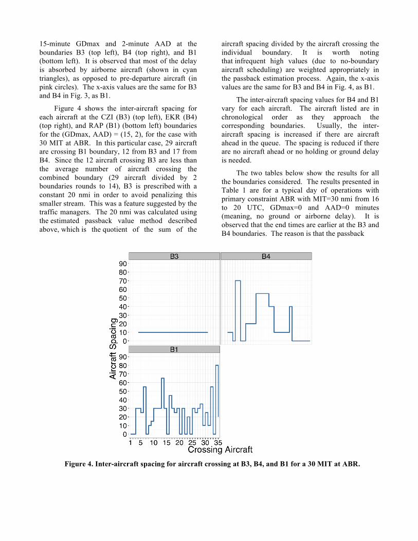
Figure 4 shows the inter-aircraft spacing for each aircraft at the CZI (B3) (top left), EKR (B4) (top right), and RAP (B1) (bottom left) boundaries for the (GDmax, AAD) = (15, 2), for the case with 30 MIT at ABR. In this particular case, 29 aircraft are crossing B1 boundary, 12 from B3 and 17 from B4. Since the 12 aircraft crossing B3 are less than the average number of aircraft crossing the combined boundary (29 aircraft divided by 2 boundaries rounds to 14), B3 is prescribed with a constant 20 nmi in order to avoid penalizing this smaller stream. This was a feature suggested by the traffic managers. The 20 nmi was calculated using the estimated passback value method described above, which is the quotient of the sum of the

aircraft spacing divided by the aircraft crossing the individual boundary. It is worth noting that infrequent high values (due to no-boundary aircraft scheduling) are weighted appropriately in the passback estimation process. Again, the x-axis values are the same for B3 and B4 in Fig. 4, as B1.

The inter-aircraft spacing values for B4 and B1 vary for each aircraft. The aircraft listed are in chronological order as they approach the corresponding boundaries. Usually, the inter-aircraft spacing is increased if there are aircraft ahead in the queue. The spacing is reduced if there are no aircraft ahead or no holding or ground delay is needed.

The two tables below show the results for all the boundaries considered. The results presented in Table 1 are for a typical day of operations with primary constraint ABR with MIT=30 nmi from 16 to 20 UTC, GDmax=0 and AAD=0 minutes (meaning, no ground or airborne delay). It is observed that the end times are earlier at the B3 and B4 boundaries. The reason is that the passback

Figure 4. Inter-aircraft spacing for aircraft crossing at B3, B4, and B1 for a 30 MIT at ABR.

specification ends at the time when the last aircraft crosses ABR. The average delay values suggest that this is not an unreasonable solution for passback to upstream facilities and would be imposed by traffic managers in current operations for two merging streams. Table 2 shows results for the same scenario, but with GDmax=15 and AAD=2 minutes. It is observed that the computed passbacks are actually less than the 30 MIT imposed at ABR. It is interesting to note that the passback values are much lesser with the introduction of just a 2-minute AAD. The traffic managers recognize this and hence desired to have a model that can compute the passback values with AAD. The GDmax allows them to provide an additional control with not too much delay for any particular flight operator. Table 2 indeed, validates their intuition that a small amount of AAD can help them manage the downstream constraint effectively and efficiently. It is recognized that the traffic conditions under which a 30 MIT is imposed at ABR, may not be equivalent to the traffic density considered here.

The results in Table 1 and 2 were obtained by running the model in the Rapid Evaluation Mode described earlier. The question that needs to be answered is that when these values are imposed, what are the realized-delay minutes for all affected flights.

Figure 5 shows the difference in total delay computed by REM and simulated in FACET for the case in Table 1, with GDmax and AAD of 0 min. The model was run for MIT values of 30, 40, 50, and 60 at ABR for traffic on CAN_1_East. The values estimated by the REM are shown in red. The simulated delay values obtained by imposing the computed passback at the corresponding boundaries are shown in blue. It is observed that the simulation produces delay values very close to the REM model estimate of 1385 minutes (see Table 1, B1 Total delay). The trend continues as the MIT value at ABR was increased up to 60 nmi.

Once these results were obtained, examination of how the incurred delays compared for various simulation runs was conducted. A comparison of total delays for aircraft flying in FACET on the CAN_1_East versus on their original (unperturbed) flight plans showed that flying on the Playbook route introduced a total delay of 905 minutes. If the MIT of 30 nmi was imposed at ABR, that introduced a delay of 821 additional minutes over the Playbook route delay. Imposing the passback restrictions with no holding and no ground delay, introduced an additional delay of 1225 minutes over the Playbook route delay. If the passback restrictions are computed using 15 minutes of maximum ground delay and 2

Table 1. Results for 30 MIT at ABR with (GDmax, AAD) = (0, 0) min.

Fix (Boundary)

Passback values (nmi)

Start time (UTC)

End time (UTC)

# AC Aircraft delayed

Total delay (min.)

Avg. delay (min.)

Min delay (min.)

Max delay (min.)

RAP (B1) 30 16:17 20:00 44 44 1385 31.48 2 56

CZI (B3) 55 16:03 18:46 15 11 65 4.33 0 15

EKR (B4) 50 16:09 19:26 17 17 348 20.47 11 34

Table 2. Results for 30 MIT at ABR with (GDmax, AAD) = (15, 2) min.

Fix (Boundary)

Passback values (nmi)

Start time (UTC)

End time (UTC)

# AC Aircraft delayed

Total delay (min.)

Avg. delay (min.)

Min delay (min.)

Max delay (min.)

RAP (B1) 20 16:17 19:59 44 36 754 16.76 0 40

CZI (B3) 10 16:03 18:03 12 2 3 0.25 0 2

EKR (B4) 20 16:09 18:02 17 9 30 1.76 0 9

minutes of absorbable airborne delay, the delay introduced over the Playbook route delay is reduced to 769 minutes from 1225 minutes.

Thus, computing passback values with no AAD causes a delay penalty of (1225-769=) 456 minutes. Also, not passing back restrictions causes an additional delay penalty of (821-769=) 52 minutes. It can be concluded that the MIT passback restrictions incorporating GDmax and AAD parameters, provide a good mechanism for traffic managers to handle the imposed constraint (at ABR) with appropriately requesting passback restrictions from the upstream facilities (at B1, B3, and B4) based on the current traffic conditions and not from a historical value.

Future Work Although results are mainly presented for the

CAN_1_East scenario for a set of imposed MIT value (of 20 and 30 nmi), it has been run for many other MIT values. It has also been run for two other Playbook routes, West_Vulcan (VUZ) and Florida to Northeast (FL2NE1). Some of these runs have been shown to traffic managers. The feedback received from the managers has been incorporated here but it’s an evolutionary process. Additional feedback from traffic managers is being obtained and the model will be improved as needed.

It is difficult to validate the model with real traffic, other than with sample scenarios presented here. The only validation for operational use can be through traffic manager feedback. One option is to develop a standalone module with this model that can be integrated with a traffic management system. This could be done using an Application Programming Interface to reduce the overhead of integrating the module with a real system. Work is in progress to develop such a standalone module. The results of that effort will be presented in a future paper.

Conclusions Traffic managers in the National Airspace

System frequently use the Miles-in-Trail traffic management initiative to handle downstream airport and airspace constraints. A model has been developed so the imposed initiative can be handled by passing some restrictions upstream to help the current facility. A previously published model was improved upon and results for two sample traffic and one real traffic scenarios were presented. Based on traffic manager feedback, the required parameters for handling traffic have been incorporated in the model and the model performs better than previous models. Additional testing would be required for this ongoing work.

Based on the results presented here, it can be concluded that the model computes passback restriction values which are more efficient for the current traffic (as opposed to historically used passback values) and do not introduce additional delay. Thus, this Mile-in-Trail passback restrictions model for any real traffic should aid the traffic managers in addressing the required passback values for that traffic.

References [1] Sridhar, B., Chatterji, G., Grabbe, S., and Sheth, K., “Integration of Traffic Flow Management Decisions”, AIAA Guidance, Navigation, and Control Conference, Monterey, CA, Aug. 2002.

[2] Bilimoria, K. D., Sridhar, B., Chatterji, G., Sheth, K. S., and Grabbe, S., “FACET: Future ATM Concepts Evaluation Tool,” Air Traffic Control Quarterly, Vol. 9, No. 1, 2001, pp. 1–20.

Figure 5. Total delay comparison of

passback restriction values between REM and simulation.

[3] Wanke, C., Berry, D., DeArmon, J., et al., “Decision Support for Complex Traffic Flow Management Actions: Integrated Impact Assessment,” AIAA Guidance, Navigation, and Control Conference, Monterey, CA, Aug. 2002.

[4] Grabbe, S. and Sridhar, B., “Modeling and Evaluation of Miles-in-Trail Restrictions in the National Airspace System,” AIAA Guidance, Navigation, and Control Conference, Austin, TX, Aug. 2003.

[5] Kopardekar, P., Green, S., Roherty, T. and Aston, J., “Miles-in-Trail Operations: A Perspective,” AIAA Guidance, Navigation, and Control Conference, Denver, CO, Nov. 2003.

[6] Ostwald, P., Topiwala, T., and DeArmon, J., “The Miles-in-Trail Impact Assessment Capability,” AIAA Aviation Technology, Integration, and Operations Conference, Wichita, KS, Sep. 2006.

[7] DeArmon, J., Wanke, C., and Berry, D., “Validation of the Miles-in-Trail Function in a Traffic Flow Management Concept Prototype,” AIAA Aviation Technology, Integration, and Operations Conference, Virginia Beach, VA, Sep. 2011.

[8] Sheth, K., Gutierrez-Nolasco, S., and Petersen, J., “Analysis and Modeling of Miles-in-Trail Restrictions in the National Airspace System,” AIAA Aviation 2013, Los Angeles, CA, Sep. 2013.

[9] Volpe National Transportation Systems Center, “Enhanced Traffic Management System (ETMS) Functional Description,” U.S. Dept. of Transportation, Cambridge, MA, Mar. 1999.

Acknowledgements The authors wish to thank FAA traffic

managers at the Air Traffic Control System Command Center and Volpe National Transportation Center personnel for their valuable feedback in the development of the current model.

Email Addresses Kapil Sheth, Kapil.Sheth@nasa.gov

Sebastian Gutierrez, Sebastian.A.GutierrezNolasco@nasa.gov

33rd Digital Avionics Systems Conference October 5-9, 2014