Development of Citywide Microscopic Models: A Case Study 

Ravi Ambadipudi, PE* Burgess & Niple Inc. 5085 Reed Road Columbus, OH 43220 614-459-2050 (voice) 614-451-1385 (fax) rambadipudi@burnip.com Steve Thieken, PE, PTOE Burgess & Niple Inc. 5085 Reed Road Columbus, OH 43220 614-459-2050 (voice) 614-451-1385 (fax) sthieken@burnip.com * Corresponding Author

Word Count: 2515

 

Abstract 

This paper summarizes the procedure adopted for the development and validation of a large-scale microscopic model, the city-wide microscopic model for the City of Dublin, Ohio. The process used takes advantage of the API’s available in the commonly used modeling tools to minimize the effort required to develop a large microscopic model. The benefits of developing large-scale microscopic models that are compatible with the regional travel demand models along with some challenges encountered in the process are also discussed.

 

  Page 2 

Introduction 

Until recent times travel demand modeling and traffic operational analyses were treated as two distinct components of transportation network modeling. Travel demand models are mostly referred to as “regional” models, as the abstract network represented by them typically spans multiple jurisdictions. The application of travel demand models was mostly limited to a “big picture” analyses. The past decade has seen an increase in the use of microscopic simulation tools to study “detailed” traffic operations on transportation networks of limited size. Software developers also treated the markets for travel demand analyses and traffic operational analyses as two separate segments; and carried out the development of mutually exclusive software modules. For instance, travel demand modeling software tools like TranPlan, TP+, and TransCAD were available and used in the United States for a long time without their respective microscopic analyses modules DynaSim and Transmodeler. On a similar note, the popular microscopic modeling tool VISSIM was used both in academia and practice for a long time without the availability of its macroscopic counterpart VISUM in the United States. This trend seems to have vanished with an increased effort from the software developers to provide tools that not only retain their core strengths but can also exchange valuable information with their counterparts. Further, the availability of API’s and scripting languages increases the potential for exchange of information across the different software development platforms used by the different vendors. This welcome change enables the development of a “big picture” model with a compatible “detailed” model. Moreover, it enables a faster development of microscopic models for larger networks which earlier were considered expensive by several agencies due to the detailed network representation required.

The availability of a large-scale microscopic model opens up a wide range of opportunities for detailed analyses and scope for the analyses of a wide variety of what-if scenarios. This paper summarizes the procedure adopted for the development and validation of one such large-scale microscopic network, the city-wide microscopic model for the City of Dublin, Ohio. The travel demand model for the City was developed using the Cube Voyager platform and a compatible microscopic model was developed using the popular VISSIM model. The abstract network information in CUBE Voyager was imported to VISUM using custom software modules and was subsequently exported to VISSIM using the automated processes in VISUM.

The remainder of the paper is organized as follows. A description of the study background is followed by a brief description of the procedure adopted. Ensuing discussion includes some challenges encountered in the process and the potential applications of the different models that were developed for the City.

  Page 3 

1. Study Background 

The City of Dublin, located in Central Ohio is a suburb of the City of Columbus. The City has witnessed an explosive growth in terms of population, employment and land use in the past two decades. The core residential area of the City is in general bounded by the limited access facility US 33 to the south and the Scioto River to the east. Access to the major employment facilities in the area is limited by the few bridges, across the freeway system and the river, which connect the residential core to the employment centers. This combined with the rapid growth the City is experiencing will have a major impact on the traffic volumes on the freeway system and the principal arterials in the area. At full build-out, the City is expected to experience a 71 percent growth in employment, 27 percent growth in population, and 36 percent growth in households (1)

The older version of the travel demand model for the City, in EMME\2, was not meeting the City’s analyses requirements. In addition, its incompatibility with the local MPO’s regional model, which was developed using the Cube Voyager platform, necessitated the development of a new travel demand model for the City. The City’s traffic and transportation staff also envisioned the need for a compatible microscopic model that enabled the study of different traffic and land-use scenarios the City was exploring to serve the increasing needs of the City’s growing transportation demands.

Burgess & Niple Inc. was commissioned by the City to develop these transportation network models. Model development was undertaken as a two-phase process. The first phase included the development of the travel demand model for the City, for the existing (2004) and future (2030) land-use conditions. The second phase of the model development involved conversion of the macroscopic travel demand model elements into a compatible microscopic model.

2. Model Boundaries 

Figure 1 illustrates the boundaries for the travel demand model and the microscopic model. The travel demand model boundary includes the City’s corporate limits and extends to include the nearest municipalities on the fringes. The microscopic models’ network boundary, also shown in Figure 1, represents approximately 36-square miles and includes the City’s corporate boundaries in its entirety. Existing year microscopic model boundaries were expanded to include major centroid-zone connectors near the City boundaries. The northern boundary of the model extends to the vicinity of Jerome Township and City of Powell. The network is generally bounded by the Cemetery Road Corridor in the City of Hilliard on the south, Sawmill Road corridor on the east and Houchard Road on the west. The network includes two freeway facilities, I-270 between Sawmill Road and Cemetery Road, and US 33 between Frantz Road and US 42. In all, the

  Page 4 

existing year model is comprised of seven freeway interchanges and over 300 arterial intersections, 80 of which are signalized.

3. Travel Demand Model  The Dublin travel demand model is a traditional four-step planning model. Developed in the Cube Voyager platform, it consists of the four steps of trip generation, trip distribution, mode choice, and traffic assignment. It is a 24-hour model with three periods, AM peak period, PM peak period and off-peak period. Traditional mode choice models include public transit, and non-motorized modes such as biking and walking. It was determined that a full mode choice model for the City was unnecessary due to the demographics of the area. “Typical” residents of the City are upper income, leading a family-oriented life style. This leads to a minimal use of public transportation modes and minimal use of non-auto modes apart from purely recreational purposes. The bulk of public transportation users in the region bounded by the Dublin model are workers commuting from outside the model area. Therefore, the current model includes only vehicle occupancy. However, the model is structured in such a manner that a mode choice component can be added, if necessary. The structure of the Dublin travel demand model is illustrated in Figure 2.

4. Microscopic Model 

The microscopic models for the study area identified in Section 2 were developed for the AM and PM peak hours. At the study’s inception (early 2006), it was decided to use a thoroughly tested and widely used microscopic modeling platform to develop the City-wide microscopic model. DynaSim, Cube Voyagers microscopic component was still embryonic and had limited usage in the industry. Therefore, it was decided to develop the microscopic model in VISSIM which at the time was more widely used. The decision necessitated the availability of tools for efficient transfer of network information from CUBE Voyager to VISSIM to avoid a repeat of time-consuming network coding in VISSIM. To accomplish this task, scripts and tools, developed using the Python scripting language and Visual Basic, were used to import the CUBE Voyager network data into VISUM, the macroscopic component of VISSIM. VISUM has an internal engine that can automate network generation in VISSIM. A detailed description of the tools used for transfer of information from CUBE Voyager to VISSIM is beyond the scope of this paper.

4.1 Data Used The data used to develop the microscopic model included aerial photographs for geometry, traffic counts, posted speed limits, and intersection control data. Automated Traffic Recorders (ATR) in the form of loop detectors are installed on some locations of the freeway facilities in the model boundary. Due to the scope of the network, extensive manual field counts provided by the City were used to supplement the limited ATR data available from the DOT. Figure 3

  Page 5 

displays the location of available peak hour traffic data for the arterial corridors in the model boundary. Each intersection on a large-scale network has its own peaking characteristic. The available intersection count information was pre-processed, using custom tool kits, to determine network-wide AM and PM peak hours. The peak hour was identified as the time during which most intersections in the network peaked.

Speed data, at key locations on the freeway corridor and some important arterial roads, was obtained using the floating-car method. The method essentially consisted of sending out observers in vehicles equipped with GPS devices to measure speeds at pre-identified locations. In addition to speeds on critical roadways, this method also provided travel time measurements for the selected travel segments along the freeway and arterial corridors.

Traffic volume data was used to calibrate the model parameters and the travel time measurements were used to validate the model.

4.2 Demand Description For models of the subject network, considered large-scale, travel demand was specified in the form of OD-matrices. OD-matrices for the sub-area network imported from CUBE Voyager were adjusted using the matrix estimation process, TFlowFuzzy, in VISUM. The estimated matrices were used in the microscopic model in a dynamic traffic assignment (DTA) setting. The use of OD-matrices and DTA processes maintained a one-to-one relationship with the planning model and ensured the model’s eventual potential for a wide-variety of scenarios including diversions due to lane-closures/construction, traffic impact studies for wide areas due to significant developments, test of ITS techniques etc., The sub-area network for the existing year consisted of 290 TAZs. Approximately 60,000 private auto trips are made during the AM and PM Peak hours.

4.3 Modeling Procedure  The modeling procedure adopted has the following major steps:

Convert the travel demand model from CUBE Voyager for the model area into VISUM file Perform OD-matrix estimation in VISUM Run a traffic assignment in VISUM using estimated OD-matrix. Export the VISUM network and estimated OD-matrix to VISSIM. Run the VISSIM simulation with dynamic assignment and calibrate the model as needed Validate VISSIM model

Detailed description of the individual steps included in the model development process, dynamic traffic assignment process, calibration, and validation exercises follows the process outlined in a similar work by the author (2). Interested parties may contact the author for technical documentation for this study.

  Page 6 

5. Goodness­of­fit of the VISSIM Models Figure 4 shows a scatter plot between observed counts and VISSIM simulated volumes for the AM Peak hour. Figure 5 shows a scatter plot between observed counts and VISSIM simulated volumes for the PM Peak hour. The overall correlation coefficient value is 0.97 for the AM Peak and 0.95 for the PM Peak, which is reasonable considering the size of the model and the disparate data sources for original counts.

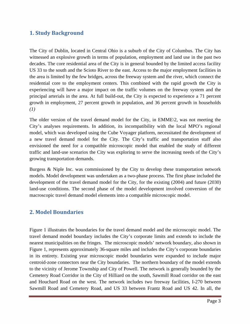
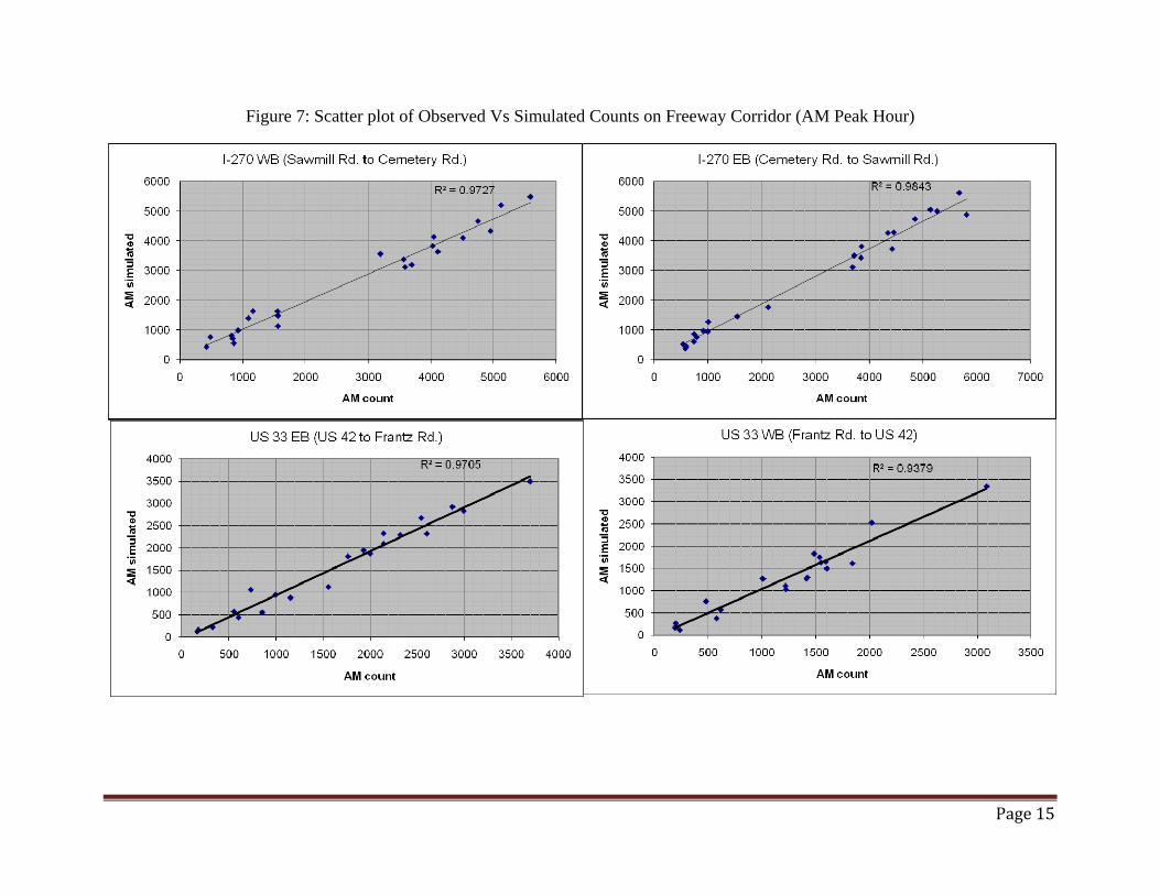
To gain an in-depth insight, the overall model output was divided into five different corridor sets, one for arterials and four for freeways, ramps. The four freeway corridor divisions were I-270 NB, I-270 SB, US 33 EB and US 33 WB. Figure 6 shows the scatter plot for the arterial segments. Figure 7 shows the scatter plot for the freeway corridors in the AM peak hour and Figure 8 shows the scatter plot for the freeway corridors in the PM peak hour. The results suggest that the model performs exceptionally well for high volume-bins and moderately for low-volume bins. Further scrutiny into these results indicated that the model failed to match field observations in areas with high variance of observed traffic volumes on a daily basis (due to varying congestion patterns).

5.1 Speed Profiles In addition to the aforementioned statistics, observed and simulated speed profiles along the freeway corridor were compared. Sample results are summarized in Figure 9. As evident from this figure simulated speed profiles follow the actual speed profiles closely. Apart from this, average speeds on select arterial segments were compared as well. These results are summarized in Figure 10. Once again the simulated average speeds were close to the observed average speeds on the selected arterial segments.

5.2 Validation Travel time data obtained using the floating car method was not used in the calibration process and hence was used as independent measurements to validate the model. Average travel times obtained from the model were compared to these values. These values are summarized in Figure 11. As can be observed from this figure, travel time measurements on arterial segments (measurements 2, 3, 4, 5, 8, 9, 10 and 11) showed more errors than those on freeway corridors (measurements 1, 6 and 7). This was attributed mostly to greater deviation of speeds on arterial corridors from the posted speed limits and better signal coordination in the field. It is possible to minimize some of these errors with better speed calibration. However, it would require more detailed information for speeds in the study area. The error on the freeway travel time segments was within 10 percent in all four cases

6. Benefits, Challenges and Future Direction It was discovered that with the use of customized software modules and tool kits, it is possible to exchange data between the different modeling tools used in the industry. This in turn aids in the

  Page 7 

efficient development of large-scale microscopic models, opening up the potential to test a wide-range of what-if scenarios that in the past was impossible as as it was perceived to be expensive and time consuming. Examples of potential applications of the validated models developed for the City range from a simple scenario like “lane closures due to construction” to a complex scenario like “effects of a regional ITS system” on the local transportation network.

Detailed modeling of large networks requires the use of several tools as all the required tasks cannot be usually accomplished using a single tool. Practitioners need to be proficient in several traffic analysis tools and be knowledgeable in the theoretical and mathematical concepts that form the backbone of the different programs. Data requirements for large-scale models are extensive. Gathering field data for such models is a laborious and time consuming process. Although computing power has improved during the past few decades, model convergence still takes substantial time for large-scale transportation networks. Calibration of large-scale networks is a challenge. It is impossible to fine-tune all the parameters that the model provides. Experienced practitioners know which parameters make the most difference to the models which results in appropriate behavior for local conditions. Educating the end-user and maintaining the models to keep up with the pace of software development can be challenging.

The City of Dublin intends to make extensive use of the models developed to study the effects of land-use changes and roadway improvements in the near-term. Where feasible, sub-area networks of the validated microscopic models will be extracted for detailed analyses of target corridors. It is anticipated that more uses for the validated models will become apparent as the region grows especially as travel demand management and ITS applications become more prevalent.

References 

1. Land Use and Long Range Planning, City of Dublin, Ohio, http://www.dublin.oh.us/planning/community/index.php, Accessed November 6, 2009.

2. Ambadipudi, R., Dorothy, P., Kill. R., Development and Validation of Large-Scale Operational Models, Proc., 85th Annual Meeting of the Transportation Research Board, Washington, DC, Transportation Research Board of the National Academies, Washington, DC, 2005.

  Page 8 

List of Figures 

Figure 1: Model Boundary

Figure 2: Travel Demand Model Structure

Figure 3: Peak Hour Count Summary

Figure 4: Scatter plot of Observed Vs Simulated Counts (AM Peak Hour)

Figure 5: Scatter plot of Observed Vs Simulated Counts (PM Peak Hour)

Figure 6: Scatter plot of Observed Vs Simulated Counts on Arterial Corridor

Figure 7: Scatter plot of Observed Vs Simulated Counts on Freeway Corridor (AM Peak Hour)

Figure 8: Scatter plot of Observed Vs Simulated Counts on Freeway Corridor (PM Peak Hour)

Figure 9: Sample Freeway Speed Profiles (Observed Vs Simulated)

Figure 10: Average Speed on Select Arterial Corridors (Observed Vs Simulated)

Figure 11: Travel Time Comparisons (Observed Vs Simulated)

Figure 1: Model Boundary

  Page 10 

Figure 2: Structure of the Dublin Travel Demand Model

Demographic

Economic and Land Use

Network Level-of Service

Pre-Generation Submodels

Workers/HH

Auto Ownership Children/HH

Trip Generation

HBWork HBShop HBRec HBOther NHB HBSchool HBColl

Peak Factoring (AM, PM, OP)

Peak Period Trip Distribution

Off –Peak Period Trip Distribution

Peak Period Mode Choice

Off-Peak Period Mode Choice

Time-of-day Factoring

Vehicle Trip Assignment

  Page 11 

Figure 3: Intersection Count Locations

FULL COUNT (2008)

PM COUNT ONLY (2008)

FULL COUNT (2004)

  Page 12 

Figure 4: Scatter plot of Observed Vs Simulated Counts (AM Peak Hour)

R² = 0.9754

0

1000

2000

3000

4000

5000

6000

0 1000 2000 3000 4000 5000 6000 7000

AM Sim

ulated

AM Count

AM Peak Hour (Observed Vs Simulated)

  Page 13 

Figure 5: Scatter plot of Observed Vs Simulated Counts (PM Peak Hour)

R² = 0.9638

0

1000

2000

3000

4000

5000

6000

0 1000 2000 3000 4000 5000 6000

PM Sim

ulated

PM Count

PM Peak (Observed Vs Simulated)

  Page 14 

Figure 6: Scatter plot of Observed Vs Simulated Counts on Arterial Corridor

R² = 0.7841

0

500

1000

1500

2000

0 500 1000 1500 2000

AM Sim

ulated

AM Count

AM Peak (Observed Vs Simulated)Arterial Corridors

R² = 0.8961

0

500

1000

1500

2000

2500

0 500 1000 1500 2000

PM Sim

ulated

PM Count

PM Peak (Observed Vs Simulated)Arterial Corridors

  Page 15 

Figure 7: Scatter plot of Observed Vs Simulated Counts on Freeway Corridor (AM Peak Hour)

  Page 16 

Figure 8: Scatter plot of Observed Vs Simulated Counts on Freeway Corridor (PM Peak Hour)

R² = 0.9859

0

1000

2000

3000

4000

5000

6000

0 1000 2000 3000 4000 5000 6000

PM S

imul

ated

PM Count

I-270 WB (Sawmill Rd. to Cemetery Rd.)

R² = 0.9445

0

1000

2000

3000

4000

5000

6000

0 1000 2000 3000 4000 5000 6000

PM

sim

ulat

ed

PM Count

I-270 EB (Cemetery Rd. to Sawmill Rd.)

R² = 0.7906

0

500

1000

1500

2000

2500

3000

3500

0 500 1000 1500 2000 2500 3000

PM

sim

ulat

ed

PM Count

US 33 EB (US 42 to Frantz Rd.)

R² = 0.9569

0

500

1000

1500

2000

2500

3000

3500

4000

4500

5000

0 500 1000 1500 2000 2500 3000 3500 4000 4500

PM s

imul

ated

PM Count

US 33 WB (Frantz Rd. to US 42)

  Page 17 

Figure 9: Sample Freeway Speed Profiles (Observed Vs Simulated)

0.00

10.00

20.00

30.00

40.00

50.00

60.00

70.00

80.00

Sawmill Road EB 161 Offramp

Tuttle Offramp

Tuttle Onramp

Cemetery Road

Spee

d (m

ph)

I‐270 WB (Sawmill Rd to Cemetery Rd)‐AM Peak Hour

Observed

Simulated

0

10

20

30

40

50

60

70

Sawmill Road EB 161 Offramp

Tuttle Offramp

Tuttle Onramp Cemetery Road

Spee

d (m

ph)

I‐270 WB (Sawmill Rd to Cemetery Rd)‐PM Peak Hour

Observed

Simulated

50.00

52.00

54.00

56.00

58.00

60.00

62.00

64.00

66.00

Cemetery Road

Tuttle Offramp

Tuttle Onramp

EB 161 Offramp

161 Loop Ramps

WB 161 Onramp

Sawmill Road

Spee

d (m

ph)

I‐270 EB (Cemetery Rd to Sawmill Rd)‐AM Peak Hour

Observed

Simulated

0

10

20

30

40

50

60

70

Cemetery Road

Tuttle Offramp

Tuttle Onramp

EB 161 Offramp

161 Loop Ramps

WB 161 Onramp

Sawmill Road

Spee

d (m

ph)

I‐270 EB (Cemetery Rd to Sawmill Rd)‐PM Peak Hour

Observed

Simulated

  Page 18 

Figure 10: Average Speed on Select Arterial Corridors (Observed Vs Simulated)

31 31 3235

2327

24

34

1 2 3 4

Sample Arterial Speeds (Observed Vs Simulated)PM Peak Hour

Observed (PM Peak) Simulated (PM Peak)

  Page 19 

Figure 11: Sample Travel Time Comparisons (Observed Vs Simulated)

905

467

375

618 624

380 376

513

372

721

542

883

690

506

861

743

359 345

509

620

810

562

1 2 3 4 5 6 7 8 9 10 11

Travel Time (s) Measurements on Select Corridors

Measured Simulated