CHAPTER - FIVE

Development of an RMS Detector

5.1) mrnooucrron

in this chapter the details of the developed rms detector arevpresented.The detector has been designed for the rms measurement on low and mediumfrequency, high crest factor signals. The direct rms computation technique is used.A squarer, a squarerooter and an averager are designed, fabricated and tested.The squarer design is carried out specially for high crest-factor signals, how­ever it is useful in other rms measurements also. A systematic analysis of thesquare-rooter is carried out and three adjustments are introduced to compensatefor the square-rooter errors. These adjustments have helped in extending thethe performance of the squarerooter over a wider dynamic range

5.2) SQUARER

Among the various squaring techniques, the function generator is chosenbecause it provides flexibility in shaping the error characteristic.

5.2.1) THE ABSOLUTE —- VALUE DETECTOR

The well known absolute-value circuit as shown in (Fig. 5.1) wasused along with the function generator to reduce the complexity. The absolute­value circuit needed three adjustments. (1) Zero Adjustment-by R‘ (Fig. 5.1)(2) Two adjustments were introduced to make the circuit perform identically on

both positive and negative signals; low-level performance was adjusted by R,’and high -level performance was adjusted by Fl-, .

For stable operation of the absolute-value circuit as well as otherblocks, using operational amplifier. it is essential that the amplifier should have

_._59__

sufficiently low noise and drift. One method of compensating for the differencein temperature coefficients of the input bias currents and thereby controlling theresulting drift was worked out by the Author while in Russia (Ref. 1).

The DC _tests on the fabricated absolute-value circuit showed .thatthe circuit could be trimmed to have a dynamic range of 3 decades (4mV to4V) with a percentage error of i 0.3 °/0. The frequency tests showed thatthe circuit had a flat response upto 10 kHz.

5.2.2) THE SQUARE —~ FUNCTION GENERATION

The function generator approximates the curve y = xi‘ . (curve 3,Fig. 5.2), by a series of straight lines which must lie in the region boundedby the two curves

y1=x2+2-C-xy2 = x—’- —— 2 - C - x

(curves 2 and 4 in Fig. 5.2)

'C‘ is the maximum permissible absolute error in rms computation correspondingto the approximation error.

Different constraints, like the maximum permissible error of approximationand least mean square error, appear (Ref. 2) in the function generator designs­In the present case however, the constraint is unique; the minimum number ofsegments for a given squarer-error characteristic, or the peak segment errorproportional to the input level.

It is a common practice (Ref. 2) to use graphical methods forapproximating the well-defined functions by a set of straight lines. On theother hand, the analytical methods provide more design flexibilities, A goodcompromise is made between the two. The straight line giving the maximumsegment length is choosen graphically; whereas its constants are determinedanalytically. The design is first carried out for a convenient input span of Oto 10 units with a corresponding output span of 0 to 100 units. Suitablescale factors can then be introduced to use the design for the actual inputand the corresponding output spans.

__6O__.

5.2.3) THE DESIGN OF THE i'th SEGMENT '

It is obvious that the straight line, with its end points on oneboundary curve and just touching the other boundary curve (as shown in Fig.5.2, curve 1) is the one with maximum segment length. Assuming the startingpoint (a) to be known the straight line ab can be completely determined(Appendix VI). The abscissa x1i of the tangent point is given by

Xlr = X i-1 + 2 \lC ' X i- 1

The slope a i = 2x; i + 2C

The segment length L = 4 J(Cx1i + C2)

The abscissa (xi ) of the end point of the i'th segment

Xi --'= ><r-1 + L

Thus the i'th segment is completely designed to have (i) maximum segmentlength and an error characteristic. Such that the resulting peak rms measurementerror is exactly C units (the derivations of the formulae are given in theappendix Vl).

This design procedure is followed for all the segments except thefirst one. The first segment needs a special consideration. Firstly, the squarererror must be zero at zero input, Secondly the boundary curves should be

2modified as per the expected squarer thereshould error Co caused by thenoise and drift.

5.2.4) THE DESIGN OF THE FIRST SEGMENT

The boundary curves are (Curves 2 Er 4 in Fig. 5.3)

2Y1='*X2_Co

2and ya == x2 + C0;

.._.61_..

2where Co = constant threshold error, The approximating straight line, ob‘, isfully defined by (Please see the appendix Vll)

(1) the slope a1 = 2x11,

(2) the abscissa of the tangent point

X1] 7- Co

and the abscissa of the end point

X1 Z (1 "I' V2) Co

5.2.5) THE RELATIONSHIP BETWEEN THE NUMBER OF SEGMENTS (n)AND THE PERCENTAGE RMS MEASUREMENT ERROR (6r).

In case of a linearly segmented approximator for a square function,the relationship between (n) and the percentage squarer error ( 55) is well­known. (Ref. 3). In the case of a nonlinearly segmented design the relationshipis not that simple. The Author has worked out the relationship (Ref. 4) inthe tabular form (table T. 5.1). A flow-chart used in determination of thistable is given in the appendix Vlll. A squarer design with 0.3% rmsmeasurement error was selected for the 0.5 ‘7, rms measurement.

5.2.6) THE CIRCUIT IMPLEMENTATION

In the actual circuit the input to the squarer (Vx) ranged from 0to 8 volts, limited by the saturation characteristics of the absolute- valuecircuit used. The output of the squarer (vy) was limited to 6 volts by themaximum input characteristics of the averager block used. The following scalefactors were introduced :

K, e V,/x r= 0.8K, = VYIV = 0.06

_.62_.

The resulting modified version of the design was then as given below:1) Break Point of the i'th segment

Vat-1 = O-8 Xi--1

2) Slope of the i'th segment

av; = 0.075 ai

3) The length of the first segment

VB; = 0.8 x1

4) The slope of the first segment

am = 0.075 a1

The function generator was implemented by using precision feedback limiters(9 Nos.) and an adder as shown in figures (Fig. 5-4 Er Fig. 5.5) ln thisdesign, the precision feedback limiters PFL (1) to PFL (i) were in conductingstate when V, satisfied the condition, vBi.1 Q vx Q Veil whereas PFL(i + 1) to PFL (n) were in the cutoff state. Therefore, the slope S; ofthe i'th PFL is given by: Si = (av; -— avi_1). The table (T. 5.2) givesthe complete design values of all the components.

5.2.7) THE PERFORMANCE OF THE SQUARER

The fabricated function generator had 18 adjustments’ The use ofstabilized power supply to control the break points resulted in successful settingup of the squarer.

The function generator was subjected to various tests. The results ofd.c. tests showed that the actual nature of the squarer error was very muchsimilar to the designed one (Curves 1 and 2 respectively, in the figure Fig. 5.6)The square function generator had a dynamic range of O.1vo|t to 8.4 volts(d.c.) i.e about three decades with an rms measurement error of not morethan 0.4 %. the frequency tests showed that the frequency error was less than5% upto 10 kHz and 3 dB point was at 50 |<KHz. The pulse- input test,was carried out at repetition period of 20ms. The duty cycle was changed insteps and the filtered output of the squarer was found to be directly propor­tioned to the duty cycle (D) over the range of D equal to 0.25 °/1, to 50 %_

__63_.

This test proved that the filtered output of the squarer was directly proportionalto the mean square value irrespective of the duty cycle.

It must be noted that 0.25 % duty cycle is equivalent to the crestfactor of 20 thus the pulse test results proved that the squarer permitted theRMS measurement of signals with crest factors as high as 20.

5.3) THE AVERAGER. W‘: . .Two identical second order Butter Worth‘s, gain low pass filters ( Fig. 5.7 )

were cascaded. The cut off frequency was selected as 4 Hz.

The averager was subjected to a frequency test, by applying 6 V (peak)sinusoidal signal. The frequency was varied from 1 Hz to 100 Hz. The ripple wasless than a few millivolts for signals of 10 Hz and oi higher frequency. Theresponse time of the averager was about 2 seconds on 5 V step - signal.

5.4 THE SQUARE - ROOTER

It performs the two functions ; square - rooting and AD conversion. Thecircuit is shown in the figure (Fig. 5.8) and the working of the circuit ispresented by its time diagram in the figure ( Fig. 5.9)

5.4.1) THE SQUARE-ROOTER OPERATION

The basic equation is

Vin I V9, at t =-- tptherefore.

in —2'l'1"I'2 l‘VR

[Ql-J

f |-IWhefe (5) Va is the known constant voltage; -r1, 12 are the integration timeconstants of the two integrators.

thus to = K ,;\/in

__.64_._

0.5Where K = T1 T2 /VR)

The circuit was designed for 10 ms output pulse width for Vin = 3 volts.

In practice, the "output pulse width will deviate from the ideal ortheoritical value because of various imperfections in the actual working of thethree blocks; two integrators and a comparator. Certain adjustments are there­fore required to get the desired performance.

5.4.2) THE ADJUSTMENTS ON SQUARE-ROOTER

The square-rooter is a nonlinear device consisting of two integratorsand a comparator. The main sources of errors in an integrator are (Ref. 5)(1) Finite open-loop gain (A0 ), (2) the d.c offset V05 and the bias current,and (3) the limited band width of the operational amplifier.

The expressions given by Tobey Er others (Ref. 5) are reproduced below:

1) Error caused by the open-loop gain A0 in case of a step input E/s:

—t/AORC Etgee:-A,,E(1—e )---­ac

twith --- -< < 1A0 RC

Et2A er) = --—-~-—-—­

2A0 R2 C2

2) Error caused by d. c. offset V05 and the bias current la :1 1Ae.,=--fv.,sdt+——flbdt+V<>$­RC c

_._65__

3) Error caused by the finite bandwidth in case of a step input E/s:

1-Q ToAea = E (-— + e ---)RC RCWhere the open - loop frequency response is approximated by a single pole at 1 /1-o.

Thus. in general one can group the integrator errors in three groups:(1) Constant errors. (2) errors proportional to the first power of t and(3) errors proportional to the second power of t.

In the square-root circuit the net error at the output of the secondintegrator is due to the second integrators error, and the integrated error of thefirst integrator. The error in V2 can be considered to have four complements;(1) constant error (2) error component proportional to t, (3) proportional to 12and (4) proportional to t3 .

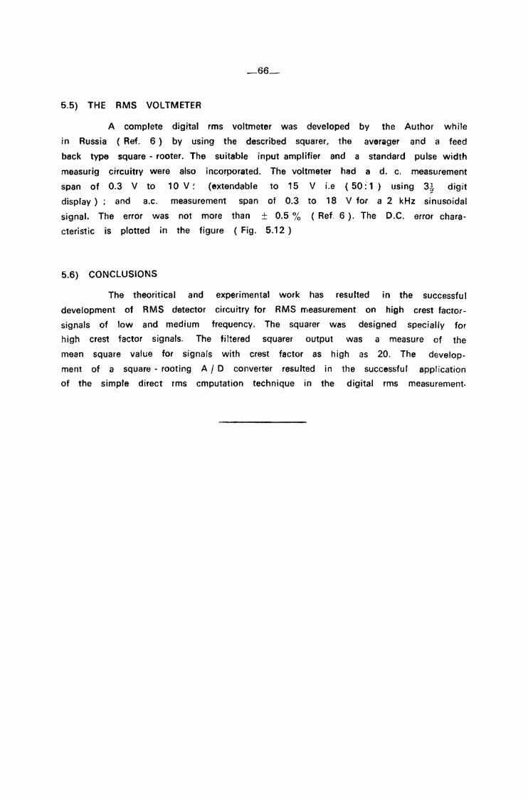
The zero adjustment as shown in the figure (Fig. 5.10) compensatesfor the constant error component, the fullscale adjustment compensates forthe error component of V._. proportional to ti (Fig. 5.10) and the half scaleadjustment (at 50 9/O of rated rms input) as shown_ in the figure Fig. 5.10for the error component proportional to the first power of time‘ It should benoted that the perfect compensation is difficult in practice because these errorcomponents are not entirely independent.

5.4.3) THE SQUARE-ROOTER PERFORMANCE

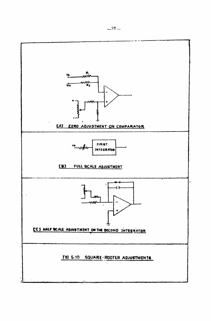
The square-rooter was fabricated and tested. The three adjustments wereintroduced and carried out. The desired performance was possible only after theproper adjustments. The square-rooter possessed an input dynamic range of 15mv to 6 v, i.e. 400 '1, with an accuracy of 0.3 %. The d.c. input-outputcharacteristic is shown in the figure ( Fig. 5.11 )

It must be noted that the dynamic range of the square-rooter limitsbasically the range of measurement and it has nothing to do with the crestfactor specification of HMS measurements.

._66_._

5.5) THE HMS VOLTMETER

A complete digital rms voltmeter was developed by the Author whilein Russia (Ref. 6) by using the described squarer, the averager and a feedback type square - rooter. The suitable input amplifier and a standard pulse widthmeasurig circuitry were also incorporated. The voltmeter had a d. c. measurementspan of 0.3 V to 10 Vt (extendable to 15 V i.e (5O:'i1) using 3.1,. digitdisplay) ; and a.c. measurement span of 0.3 to 18 V for a 2 kHz sinusoidalsignal. The error was not more than i 0.5 % (Ref. 6). The D.C. error chara­cteristic is plotted in the figure (Fig. 5.12)

5.6) comctusroms

The theoritical and experimental work has resulted in the successfuldevelopment of RMS detector circuitry for RMS measurement on high crest factor­signals of low and medium frequency. The squarer was designed specially forhigh crest factor signals. The filtered squarer output was a measure of themean square value for signals with crest factor as high as 20. The develop­ment of a square-rooting A/D converter resulted in the successful applicationof the simple direct rms cmputation technique in the digital rms measurement­

_...67._.

References

Deo P. V. , Melnikov A. G. : ‘The method of Reducing t.he drift of d.c.differential amplifiers’ Scinetific Notes : No. 8 1974, Baku ( USSR ) p. 101.( Russian )

Scott N. R. ‘Electronic Computer Technology‘ McGraw Hill KogakushaLtd. 1970 p. 72.

Howard Hamer. ‘Optimum Linear-segment function generation. AIEE Transa­ction on communication and Electronics. Part 1 Vol. 75 Nov. 1956, p. 518.

Deo P. V., Melnikov A. G. ‘Function Generator for RMS Voltmeter‘ Izv.VUZ. priborostroyeniya (Russian) Vol. No.5, 1975 p.72 (Russian)

Tobey. Graeme. Huelsman, ‘Operational Amplifiers‘ Design and Applications‘McGraw Hill Kogakusha Ltd, 1971 p-213-217.

Aliyev T. M.. Melnikov A.G., Deo P. V. ‘Digital Voltmeter of Effectivevalves’ IZV. VUZ. priborostroyeniya Vol. XIX N0. 11. 1976. p. 26. (Russian)

Approximation Segment VS RMS

TABLE T. 5.1

_._68.__

Measurement Error

.6 0.1 * 0.2 0.3 0.4 , 0 5

H I 11 7 ____ _ I.

_ . _ ... ‘ __ — _— —_ i16 1 11 A 9 6 A 7 "

1

TABLE T. 5.2

Squarer Design

V61-1I

R21

kohm Sis ' R41ii kohm

91 .Ro/ RxiR xi

kohm

A

I

\

1

2

3

4

5

6

7

8

9

° i0.1792 9

0.5325 ;

1.0807

1.s2o9 g

2.7530

3.6773 ‘

5.1340 1

6.7015

400

169

86

49.5

32.6

23.2

17.6

13.4

T!

‘ 0.0137

0.0482

0.0711

0.1071

“ 0.1431

, 0.1791

\ 0.2151

0.25110.2871

1.5

g= 5.0

5.0

. 5.86.8

8.2

10.0

A 1 5

.51

0.1

0.333

0.386

0.386

0.454

0.548

0.667

1.0

3.4

0.137

0.145

0.184

0.277

0.320

0.328

0.324

0.251

0.085

13.6

10.6

1.2

6.2

6.1

6.2

6.0

23.7

5 .

15.4 I

i‘ ‘_“OG__ ___QW_hm“Gmg hM_Dm__l___w M533‘ __w_ 0 DOR5“m_”_______‘I! II‘. |__i l\ ll% 2 MmH‘ E MN‘ JELW\ L‘ ‘ *l_ ‘ I I!‘ ‘C_F A VIM‘

___Jj1||‘ A‘ _ 4 I I H'___1M‘_ ‘____|’*Hl__w"‘ ii’ \ 7 Y ‘i ‘N __ 7;‘_ _ ‘ I _“‘ 1‘ ‘ll _“l‘ “ “ ‘ZHDI “V VII \| I I‘ ll: ‘I __ _I;_____r(0I G 6_ |Y '_'._i|fi*___ _ Q Iq? (L0 I__‘___ / M“ii! _| _l I ‘ ‘Ni N1 N H7 I L_‘¢ \‘||_I_"?‘__M___ H_ "W_Z Q © i_in . u __ _ '____ :":l___' _ _‘_ H_ T__ _‘Hlblilzw M“ My H|_“‘|_ “ ‘I :lH_|‘,lH‘wl‘_“‘l|_‘ ““‘ :“:‘I L" _ [__ _ V V iii 'W|[%{I‘E\‘\I_‘IKL‘L\\‘_‘“\H\% \ IWMI '1L_|[H “H J“ ‘ filfi ll ML: __H_d|’!W‘H" ‘ Ili ‘¢||U}_lN__|‘|‘1‘_"“‘MU‘ P‘

y ?“"*% 596$ L

._TL­

- .\M M ‘JT lkL .\ .

I "u- k. . ._ . \._ _ 1Ry QB" I " ¥&\—*'1

f_3_g,A5-3%; H e-5-4 [B] A2RE<=':»~<>~%iiFgifivwk ~

4; L‘;

&i.

|q —— PFLI N

. Y|‘_

\

A -f.ii:; ‘ _ Q;4%__1_;f 4I

. _ .

_ inf‘ ii;-‘_‘ ;4 ‘-“iii;

_ \“ - ‘A‘ _:\lx

§ PFL2 — ~ — —Y,‘ '§ PFL1 ¢i‘“ - \‘r . 1!a\ “\ =‘1 *% :PFLn “\ "

-afla3

1 FlG'S'5 SQ-jUNCT!0N' APPQQXIM L ‘% % % WWW ? _{¢N TM jwfi *M%HA V :5 __._ __.__ . ___ I ‘If-- -~~ ~- —— --— ~ ­H ' _ 11“ ‘-‘;F",_f-__1-ll‘ “ JJ 1? ‘ T I_ _— ij . :;:“:;:

‘|'!_1i_|\H“h‘_lli'M_'_'{\\ \|__ NHIW‘ \ \ i “ ‘j 1_ll_|_-\\ F N ¥ \ \ I W N} I W‘ ‘\ ‘Ml \ ‘\ \ ‘ ‘I> 1 __ R \ it é ] \ ]__:___ é|_ I é_\|é M "H ‘ l ' _|_| ‘N,_ '_M ____ ? _m¢Id %M Q1_ _ % :___i_W _% _% L Vokqd "W__ ¥ _____ u ._~ . “qi?" _ ' \ _L ~ K '%_ p s __ _’ _ _j A_ \ _ _ ?_ 1_ _ _ ___ _ __ ___ __ _ _ _r_ A 7 __ m______J_I H_ _ _i j X L,‘ i2_°___ R: ~O_g_9__ ___ac_ Q_ _ X ,’i d ’ l ~ ’ i 0 j‘ mi“F _ % i iK. ,_ __ \ ‘A \ ‘\ ‘A \ _ \ _A (‘V NH’. H _ . _ ’ >__ _N ‘ 1_\_ 1 é N l 1 _‘J‘\ I‘ A F _ _ ‘__('!_ ( H‘!f ’ _ _ L : ‘. _'_ \ V‘ u__ _ _ _ _ ’ _ mi_ _ W_ _ ’% 9_ , V ’ V _? V __ W °__;_% ‘ _ ’ __ ’ _ _’~ "_ _NH f _ p t (___’ Q __ K 3+ ti_ € ml_ _W g_hw_&h%§Iq mama AgofiwMm4:dWfl%M%w_Mi tV“ _ i ____ _ > _ _ I __ '.>. _. ‘I > _ ___ i __ _ __ _ _ _l _ _ _

r“Hur“‘H‘i Wllflt‘ I NJ!‘ k‘IH_l UI‘kPI‘_l‘_‘_ ll ‘[1 I’ I ‘ _r|r‘ II _:, V _'‘__>I1 ‘ ____RMI‘ J J _ ‘|J|1\:1 :|*PH||| ’hM '|‘H‘1U_'_'____‘h“:’l{“ NW Fir “HI 11" ' Ink F,‘ _QMS“IM“MdMy W M1 _MM8‘__Qm Mha|lU‘wU|‘l ‘HflW_P| A |“uH|.|lP‘l‘|hlJ1HH|' _ ‘“,_"WH‘: l|__"'__ti_1 _ I \__'__ ¥i;_( ""'!',""__"""‘.__‘__“‘1'_ L,” “M q“‘+wn' UHF “HIM ‘ I _ _|Hy"|"q IITLH‘, J‘ HUI L‘ ‘ _ ‘_ I‘ ]_ ‘l‘ “‘

QA“

,.'

I

1 .'I

' F

I

I‘:

l:

L5‘?

IIII I

{I

I

I

I

II

4-.__ I. -. ._L _,____~ __ _4—-.—-4._,-—__‘lr _

\

ii4!,I

. V

-;I

I.

I.

I

M — — — - — i * * —* — —~ ""77? -T7-‘ I M 7‘ — — ~ f ~ W" 7+ --- ~37- ~—R.­

if [1 sta1t'§¢¢nn0nl.1‘

I.' L

fllg *7‘?-“­

I F

"1,"I

III

II\

A

I;

‘__ I

oI~ '“ uv '

qI¢0¢ncnuqi-ti

11*-I--r --'

'_--in-pug

_ I/1 linteavam I Ar-~—---I|

:'(I'ni --4-~

’.I‘. l

I* I I U " H ITI latofldu 1 H W M“~ ‘

Q53

K.

I

I

' 5

conpqvutn

chub 1! duh

;1'17"’ -~f . Ifi=|

Q

I

I

0

3

ii?

.b¢I—

. rlr éurpd' - - -——~-b--——— ~" — -~ ‘I-~~ ._3W -_ ;';""‘- .:;-;-_ , .;_i‘_if‘_; "*"__-1-_:;r " :"1.1,:.._| . ..I_*... _ _. __*fi_ ._‘__~--r.-Y

Tina L--1»

.~'.7T_ n _ —_ qa *_'r'_-*1-V—V~V~f-:“._-_;_:_’:_ ‘,1, _ _ _ _ J m g in ‘ ‘i 7 I' " 7" ~““‘-”" "*#1“—"*‘lA-ii".‘<?:r=:<<.f'—fi““"i _. ' ' " " '

?

J'­1

.1‘

H

-"I1 \

5 F

;*r

I

I.

1.

FF

I

V

I

_,.._1._>I ___?I '1' 1 _-­

Ii

-‘F

i

1 r

I

1.‘l{LJ‘I.,I

‘k

I|

'~l

n'_

-‘rI

\

|4

‘ \

I .

‘ __. i — —~ ' -~;4—,:,,,,:-|-Q--nil -I '.;1_.' 5 7 “'*_ . ___ ,,_ _ - _ *_A-I ;,__¢_,_ __:'1;: “."i;';J — * "" 'f f __..___ __rv.-yr-—'.1\ I» —— . '

V: % V _ "sVia ' R}4- 1 ‘I

an‘‘ Q- . ,%f~Q44\!5T%"§ NI _QN(Q9!l.?1é‘R5IQ~!~

mwznmx L

%§§;3,. K ¥‘l%'»§€5_l§.A2!P5LT!!§FT

~~‘—L 4‘ * — ,4 T‘/f‘Te_'_5 _ W‘ _. _+ ;';__:*.;:_._:?___ __ *;__ _ ___ _ _ fi é _ r _._ __.

,%°;€4@i._*\I?*"" *!!'¢1,<=9T"*2=¢<!~T=2 1?11_§§.~%t2a. .:-~ L, “ _ fi gl‘ __ ___ _, ft;. I _ _l * ' * 6 _T" ‘ -_"i‘-§1i;;liH#I*';1 ;__ :_ — a *_ —‘: — "‘ ht; 5 '_ _;1_;; ’ L? ._

% jig 5-so m5_guAR%s-_3AopnnA ApJuBTn1:M_s

W é\ \\X-1;-_ l I

ir\

\ ,

(:._;‘_

i

I4

:_ J

J11

.H

ix

\\

U

W |

W

I

W

\

i

N

w

I.\­1\u

|

I

' \

4

l\I

'\1

H

‘.

§Il.

I

V.

LL-'

\

1.W

T —f,,f‘,1

ffl

1 l

W

5

jitZ:__ v w“M|HihHl_} MM“ __"!‘Lk‘l__r__“_h"_‘ [NP ‘i_¢l1i‘¢_ hJL_\\‘14[\ ‘\MWH_HHé ‘_L_‘|l_HM_ éM\PHwhWéM4_M_______ ___ __ 2 _g “tau EU“ __ _w flT ‘i C; 't 2 8.5 {N ___N 3 3 2 Md 06 3 O __ll 1Q\Jj y J \ \\ \1‘1rr [ “aimL “Bog mmdaam u___%__% mo Ww_%5mmwU¢m¢ruH__EwImO_::___0‘mE AM:___L____E__H_‘__jI__::12i__W__jA_____ \_______L _W fiLw1 L l J.‘ AM 4|_ ““f“‘[‘W‘|H“|t MU“ ‘ H “fl%IW‘rh|W vU_“__Z V*_ “\l_\_'_ _ _H|__||dL|‘ _1_ ‘L v1_‘_h|#U_H_“ \y| “|v_1‘_ __\“‘__\‘ Kl_“_k \“i_‘q‘_ '_W_\|] _¢_ ( r L____l_ fiT_I__g _H _ __ __L8“ W__ ‘ ‘ _L_J _ Q HHT$80 __J IM VJ63 _M _iH _L82 _» __T*8____m_._.6 _i I‘ H _‘ l‘l‘_|‘ ‘_{\\t.f“:‘ W W ‘ [ ‘ll Ill‘ V IN WU “\:_ ‘\ \‘ \ \I i ; I ‘ 1!“ HM‘ vi“ ‘ K‘\|H\i1“|_¢“;:|_"Ul “1]'_‘_‘ i_;“‘§__‘ Pi“ ‘U! \__ nu“ ‘HIV? “:_|“ ‘ ‘ N‘ _v‘\11h_‘ MN‘ \l _NH I“ “‘_ N‘ “ H

_ "W‘_\“‘|‘_|M"_'_" “““‘__HH'¢‘ ‘|“'_‘ _“ “‘||],“‘_‘_iw||J_“‘|d}‘]_‘ ‘L)Hw|‘W_ [ l ‘V VI _ \' ‘ I I __‘ ‘_ ‘ F ‘r V [‘ V _ _IN _ \ 3} \ i \ \ I J \ I; PI Wl‘ ‘_ ‘_[I‘N‘_‘>l‘L W_ MMMWVW MIL ‘J \id wfiamw~ ___7 + + %7_ ____> * _ _ 7é *4 LiewCflaém l &E_qgA 9°‘_ _\__i# + A* _1i'‘I. __ _A0” org fir 3 CW4 gy Q” %8__'_T% N6 G_; WI_% __|T :Li‘ 3f_fiL