Embed Size (px)
Citation preview

DEVELOPMENT OF A WING DESIGN TOOL USING EULER/NAVIER-
STOKES FLOW SOLVER
A THESIS SUBMITTED TO
THE GRADUATE SCHOOL OF NATURAL AND APPLIED SCIENCES
OF
MIDDLE EAST TECHNICAL UNIVERSITY
BY
KIVANÇ ÜLKER
IN PARTIAL FULFILLMENT OF THE REQUIREMENTS
FOR
THE DEGREE OF MASTER SCIENCE
IN
AEROSPACE ENGINEERING
DECEMBER 2005

ii
Approval of the Graduate School of Natural and Applied Sciences
______________________
Prof. Dr. Canan ÖZGEN
Director
I certify that this thesis satisfies all the requirements as a thesis for the
degree of Master of Science.
__________________________
Prof. Dr. Nafiz ALEMDAROĞLU
Head of the department
This is to certify that we have read this thesis and that in our opinion it is
fully adequate in scope and quality, as a thesis for the degree of Master of
Science.
__________________________ __________________________
Dr. A. Ruhşen ÇETE Prof. Dr. İ. Sinan AKMANDOR
Co-Supervisor Supervisor
Assoc. Prof. Dr. Sinan EYİ (METU,AEE) _____________________
Prof. Dr. İ. Sinan AKMANDOR (METU,AEE) _____________________
Dr. Ali Ruhşen ÇETE (TAI) _____________________
Assoc. Prof. Dr. Serkan ÖZGEN (METU,AEE) _____________________
Prof. Dr. M. Haluk AKSEL (METU,ME) _____________________

iii
I hereby declare that all information in this document has been obtained
and presented in accordance with academic rules and ethical conduct. I
also declare that, as required by these rules and conduct, I have fully
cited and referenced all material and results that are not original to this
work.
Name, Lastname: Kıvanç ÜLKER
Signature :

iv
ABSTRACT
DEVELOPMENT OF A WING DESIGN TOOL USING
EULER/NAVIER-STOKES FLOW SOLVER
ÜLKER, Kıvanç
M.S., Department of Aerospace Engineering
Supervisor: Prof. Dr. İbrahim Sinan AKMANDOR
Co-Supervisor: Dr. Ali Ruhşen ÇETE
December 2005, 140 pages
A three dimensional wing design tool with analysis functions has been
developed with embedded Euler/Navier-Stokes flow solver and a three
dimensional hyperbolic grid generator. A graphical user interface has
been constructed using PYTHON script language and the tool was
enhanced with pre-processing and post-processing capabilities. Analysis
and design procedures are demonstrated with automatic grid generation,
automatic series solution and automatic graphs and reports generation.
Keywords: TAIWING, wing analysis, wing design, CFD, aero. design tool

v
ÖZ
EULER/NAVIER-STOKES AKIŞ ÇÖZÜCÜSÜ KULLANARAK
KANAT TASARIM ARACI GELİŞTİRİLMESİ
ÜLKER, Kıvanç
Yüksek Lisans, Havacılık ve Uzay Mühendisliği Bölümü
Tez Yöneticisi: Prof. Dr. İ. Sinan AKMANDOR
Yrd. Tez Yöneticisi: Dr. Ali Ruhşen ÇETE
Aralık 2005, 140 sayfa
Halıhazırda bir Euler/Navier-Stokes akış çözücüsü ve bir üç boyutlu
hiperbolik ağ yaratıcı kullanılarak bir kanat tasarım ve analiz aracı yazılımı
geliştirilmiştir. PYTHON betik dili kullanılarak bir kullanıcı dostu grafiksel
arayüz hazırlanmıştır ve yazılım “işlem öncesi” ve “işlem sonrası”
yetenekleriyle donatılmıştır. Kanat analizi ve tasarımı kullanılışları
otomatik ağ üretme, otomatik çözümleme ve otomatik grafik ve rapor
üretme özellikleriyle beraber gösterilmiştir.
Anahtar Kelimeler TAIWING, kanat analizi, kanat tasarımı, HAD
hesaplamalı akışkanlar dinamiği, aerodinamik tasarım aracı.

vi
ACKNOWLEDGEMENTS
I would like to express my appreciation to Dr. Ali Ruhşen ÇETE and Prof.
Dr. İ. Sinan AKMANDOR for their support, guidance and motivation.
I am grateful to Yüksel ORTAKAYA, Hakan TİFTİKÇİ for their help,
interest and programming guidance during my learning curve of Python
script language.
Emre GÜRDAMAR is sincerely acknowledged for his support.
And thanks to my friends and colleagues who aided me during test of the
program.
This study was supported by The Scientific and Technical Research
Council of Turkey (TUBITAK) within TIDEB project of “Development of
Aerodynamic Design Tools Using Computational Fluid Dynamics”
(TIDEB3040091).

vii
TABLE OF CONTENTS
PLAGIARISM ………………………………………………………………………………….. iii
ABSTRACT ................................................................................................................... iv
ABSTRACT: DEVELOPMENT OF A WING DESIGN TOOL USING EULER/NAVIER-
STOKES FLOW SOLVER ............................................................................................. iv
ÖZ ................................................................................................................................... v
ÖZ: EULER/NAVIER-STOKES AKIŞ ÇÖZÜCÜSÜ KULLANARAK KANAT TASARIM
ARACI GELİŞTİRİLMESİ................................................................................................ v
ACKNOWLEDGEMENTS .............................................................................................. vi
TABLE OF CONTENTS................................................................................................ vii
LIST OF TABLES ........................................................................................................... x
LIST OF FIGURES......................................................................................................... xi
1.INTRODUCTION.......................................................................................................... 1
1.1 General overview .........................................................................1
1.2 PYTHON script language.............................................................3
1.3 The scope this thesis ...................................................................4
1.4 Description of chapters ................................................................5
2.TAIWING...................................................................................................................... 6
2.1 Definition ......................................................................................6
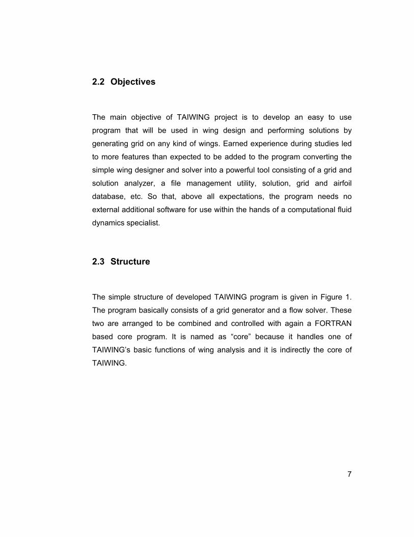
2.2 Objectives ....................................................................................7
2.3 Structure.......................................................................................7
3.GRID GENERATOR................................................................................................... 12
4.FLOW SOLVER ......................................................................................................... 20

viii
4.1 Euler/Navier-Stokes Equations and Method of Finite Differences
...................................................................................................21
4.1.1 Generalized Curvilinear Coordinate Transformations ........21
4.1.2 Thin-layer Approach ...........................................................22
4.1.3 Finite Difference Methods, Numerical Algorithms ..............22
4.2 Turbulence Models.....................................................................23
4.3 Studies of Multi-Block Approach................................................24
4.4 Metric Calculations.....................................................................29
4.5 Writing Flexible Boundary Conditions Managed From Input File ..
...................................................................................................29
4.5.1 Boundary Conditions Input File ..........................................30
4.5.2 Input File Codes and Commands .......................................32
4.5.3 Region and Directions Assignments in Boundary Conditions
and Surface Operations ....................................................................34
4.5.4 Wall Boundary Condition ....................................................37
4.5.5 Symmetry Boundary Condition...........................................38
4.5.6 Matching Boundary Condition ............................................38
4.5.7 Block Interface Matching Boundary Conditions..................40
4.6 Flexible Boundary Conditions Check in Single-block Structure 41
5.TAIWING FORTRAN SOLVER CORE....................................................................... 46
6.PHYTON INTERFACE............................................................................................... 50
6.1 Main Window..............................................................................52
6.2 Menus.........................................................................................54
6.3 Generating Grid Screen .............................................................56
ix
6.4 Solver Parameters Screen.........................................................60
6.5 Grid Loading Screen ..................................................................63
6.6 Running Screen .........................................................................64
6.7 Saving Solutions Screen............................................................69
6.8 Database Manager.....................................................................71
6.9 Patterns Manager.......................................................................82
6.10 Advisor .......................................................................................85
6.11 Options Screen ..........................................................................88
6.12 Help Screen ...............................................................................90
7.WING DESIGN........................................................................................................... 92
7.1 Validation....................................................................................93
7.2 Creating Grid Patterns ...............................................................99
7.3 Creating Advisor Criteria..........................................................100
7.4 Preparation of Solution Matrix..................................................102
7.5 Results .....................................................................................104
8.CONCLUSION ......................................................................................................... 113
REFERENCES............................................................................................................ 114
APPENDICES
A. 2-D GRID GENERATION ..................................................................................... 118
B. EULER/NAVIER-STOKES EQUATIONS ............................................................. 123
C. GENERALIZED CURVILINEAR COORDINATE TRANSFORMATION ............... 127
D. THIN LAYER APPROACH................................................................................... 130
E. FINITE DIFFERENCES METHOD ........................................................................ 132
F. METRIC CALCULATIONS ................................................................................... 134
G. BOUNDARY CONDITIONS.................................................................................. 136

x
LIST OF TABLES
TABLES
Table 1 Definitions of input parameters [ref.28]........................................................ 31
Table 2 Codes and commands of input file of TAINS program [ref.28]................... 32
Table 3 Parameters of matching boundary condition [ref.28] ................................. 39
Table 4 Modules used in TAIWING PYTHON interface ............................................. 51
Table 5 Naca0012 test wing [ref. 13 ] ......................................................................... 94
Table 6 All wing configurations selected in wing design....................................... 103
Table 7 Lift to drag ratios with different sweep and dihedral angles .................... 110

xi
LIST OF FIGURES
FIGURES
Figure 1 Basic structure of TAIWING program ........................................................... 8
Figure 2 Advanced structure of TAIWING ................................................................... 9
Figure 3 Three dimensional C-O type hyperbolic grids generated by GRID3D ...... 12
Figure 4 Example input file of GRID3D grid generator program.............................. 13
Figure 5 Grid dimensions and wing parameters....................................................... 14
Figure 6 Clustering parameters.................................................................................. 15
Figure 7 Dimensions of a 2D (clustered) hyperbolic grid generated over an airfoil
...................................................................................................................................... 16
Figure 8 Third dimension K of 3D hyperbolic grid.................................................... 17
Figure 9 Rounding of 2D grid planes at the wing tip ................................................ 18
Figure 10 A three dimensional C-O type hyperbolic grid ......................................... 19
Figure 11 Schematic of program data structure [ref.28] .......................................... 25
Figure 12 Tree structure of solver program and module where data structure is
defined [ref.28]............................................................................................................. 27
Figure 13 Starting definitions forming the last stage of solver main program
[ref.28] .......................................................................................................................... 28
Figure 14 An example boundary condition input file [ref.28]................................... 33
Figure 15 Defining systematic regions and designation of LB series values [ref.28]
...................................................................................................................................... 34
Figure 16 Subroutines converting surface definitions to double index form ……..36
Figure 17 Interpolation types [ref.28]......................................................................... 40

xii
Figure 18 Comparison of pressure distributions of CO and CH wings controlled by
input file using TAINS solver program [ref.28].......................................................... 42
Figure 19 C-H wing grid (left) and C-O wing grid (right)........................................... 43
Figure 20 H grid of Onera M6 wing [ref.28]................................................................ 43
Figure 21 Input file of Onera M6 C-H type wing grid [ref.28] .................................... 44
Figure 22 Input file of Onera M6 C-O type wing grid [ref.28].................................... 45
Figure 24 An example input file of TAIWING FORTRAN solver core....................... 48
Figure 25 TAIWING program startup screen ............................................................. 53
Figure 26 Information displayed on TAIWING main screen ..................................... 54
Figure 27 TAIWING main menu bar............................................................................ 54
Figure 28 Menu of options displayed when “NEW” button is used ........................ 55
Figure 29 Right click menu......................................................................................... 56
Figure 30 Generating grid screen .............................................................................. 56
Figure 31 Generating grid screen wing geometry and grid parameters input........ 57
Figure 32 Generating grid screen advanced grid parameters section.................... 58
Figure 33 Generating grid screen grid preview section ........................................... 59
Figure 34 A sample 3D grid model examination ....................................................... 59
Figure 35 Solver parameters screen.......................................................................... 60
Figure 36 Solver parameters screen flow conditions input section........................ 61
Figure 37 Solver parameters screen advanced flow solver modification section.. 62
Figure 38 Loading grid screen ................................................................................... 63
Figure 39 Loading grid screen sample grid summary.............................................. 64
Figure 40 Running screen solution startup............................................................... 65
Figure 41 Running screen solutions checklist and error status.............................. 65
Figure 42 Running screen initialization settings ...................................................... 66
Figure 43 Running screen global and cl residual tracking ...................................... 67
Figure 44 Running screen solution status ................................................................ 68

xiii
Figure 45 Saving solutions screen ............................................................................ 69
Figure 46 Examination of a new solution’s global (logarithmic scale) and cl
residual graphs in saving solutions screen .............................................................. 71
Figure 47 Database manager screen solution inspection........................................ 72
Figure 48 Database manager screen solution summary.......................................... 73
Figure 49 Database manager screen sample grid summary.................................... 74
Figure 50 Database manager screen sample airfoil summary................................. 75
Figure 51 Database manager screen reports and graphs wizard............................ 76
Figure 52 Database manager screen automatic PDF solution reporter sample
output ........................................................................................................................... 77
Figure 53 Sample output graph generated by database manager screen custom
solution graph generator displaying Cp distribution on a wing root....................... 78
Figure 54 Database manager screen report wizard for custom PDF report
generation.................................................................................................................... 78
Figure 55 Database manager screen custom PDF report generator sample output
...................................................................................................................................... 79
Figure 56 Database manager screen custom graph generator from multiple
solutions ...................................................................................................................... 80
Figure 57 Database manager screen 3D solution viewer sample solution grid ..... 81
Figure 58 Database manager screen 3D solution viewer ......................................... 82
Figure 59 Patterns manager screen........................................................................... 83
Figure 60 Patterns manager screen sample grid pattern ......................................... 84
Figure 61 Advisor screen............................................................................................ 85
Figure 62 Advisor screen sample advisor criterion.................................................. 87
Figure 63 Options screen general program preferences ......................................... 88
Figure 64 Options screen display preferences ......................................................... 89
Figure 65 Options screen parameter default value controls.................................... 90
Figure 66 Help screen ................................................................................................. 91

xiv
Figure 67 Naca0012 symmetric airfoil........................................................................ 93
Figure 68 A coarse grid around test wing with 80x25x18 dimensions.................... 94
Figure 69 A fine grid around test wing with 275x65x80............................................ 95
Figure 70 A suitable grid around test wing with 200x30x40 .................................... 96
Figure 71 Solution report of Naca0012 test wing at 0° angle of attack ................... 97
Figure 72 Solution report of Naca0012 test wing at 2° angle of attack ................... 98
Figure 73 Naca0012 test wing grid pattern.............................................................. 100
Figure 74 Naca0012 test wing advisor criterion...................................................... 101
Figure 75 CL versus sweep angle graph with varying dihedral angles ................. 105
Figure 76 CD versus sweep angle graph with varying dihedral angles ................. 106
Figure 77 CX versus sweep angle graph with varying dihedral angles ................. 107
Figure 78 CY versus sweep angle graph with varying dihedral angles ................. 107
Figure 79 CZ versus sweep angle graph with varying dihedral angles ................. 108
Figure 80 MX versus sweep angle graph with varying dihedral angles................. 108
Figure 81 MY versus sweep angle graph with varying dihedral angles................. 109
Figure 82 MZ versus sweep angle graph with varying dihedral angles................. 109
Figure 83 Lift to drag ratio versus sweep angle graph with varying dihedral angles
.................................................................................................................................... 111
Figure 84 Bell X-5 experimental aircraft with variable sweep from 20 degree to the
full 60 [ref. 30] ............................................................................................................ 112
Figure 85 Transformation from computational space to physical space) ............ 119
Figure 86 Example 2D cell configuration................................................................. 134
Figure 87 Vector representations on grid surfaces ................................................ 136
Figure 88 Symmetry plane........................................................................................ 139

1
CHAPTER 1
INTRODUCTION
1.1 General overview
Fluid dynamics is most often complex. The equations governing fluid flows
are non-linear, and can only be solved analytically in a few cases. While
these cases proves to be useful approximations of the real solution in many
situations, the fact is that only through scale model testing in wind tunnels,
or other experiments could more precise and detailed information be
obtained. Given that the availability of such testing is limited and that the test
is not inexpensive, many projects that might have benefited were not
subjected to fluid dynamic analysis. All this has changed in the past few
decades with the exponential growth of computer power and the application
of Computational Fluid Dynamics (CFD).
The object of CFD is to use computers to solve the previously intractable
conservation equations for fluids in order to accurately simulate flows. This
typically involves discretizing the problem in a finite set of elements, applying
the conservation of mass, momentum, energy, and chemical species (where
necessary) to these elements, placing additional boundary conditions at the
edges of the computational grids, and solving the resultant algebraic
equations in an iterative fashion. One method is to discretize the spatial
domain into small cells to form a volume mesh or grid, and then apply a
suitable algorithm to solve the equations of motion (Euler equations for

2
inviscid and Navier-Stokes equations for viscous flow). In addition, such a
mesh can be either irregular (for instance consisting of triangles in 2D, or
pyramidal solids in 3D) or regular; the distinguishing characteristic of the
former is that each cell must be stored separately in memory. Lastly, if the
problem is highly dynamic and occupies a wide range of scales, the grid
itself can be dynamically modified in time, as in adaptive mesh refinement
methods [ref. 25]. While the ideal is for CFD simulations that do not require
actual scale-model experiments, in fact, some scale-model experiments are
generally still necessary in order to validate the accuracy of the CFD code.
Still, the number of necessary experiments can be greatly reduced as
computations fill gaps between experiments and numerical models can
simulate situations that would be impossible to set-up experimentally.
Thus, computational fluid dynamics allows the analysis of fluid flow problems
in detail, faster and earlier in the design cycle than possible with
experiments, costing less money and lowering the risks involved in the
design process. This trend is only likely to grow more pronounced in the
future as computers become increasingly cheaper and more powerful while
traditional forms of testing become increasingly expensive.
A tool newly developed within this trend with the scope of aircraft wings is
TAIWING. There have been previously developed analysis tools for airfoils
like “VisualFoil Plus”, “3DFoil”, “PANDA” and “MultiSurface Aerodynamics”
designed only for fast and efficient analysis over wing cross-sections [ref.
26]. TAIWING takes the flag from these analysis software and moves it one
step forward by enlarging the scope of airfoils to complete wings. These are
generalized tools capable of analyzing any 3D objects virtually constructed
within the user interface, which are also capable analyzing wing structures
but they are not quite efficient and are not directed to the target point of
wings as TAIWING does.

3
TAIWING handles all three parts of a CFD tool:
• Pre-processing: generation of a computational model, grid generation
(handled by built-in grid generator) and specification of physical
properties of flow conditions as well as boundary condition definitions.
• Processing: to perform the computation (handled by the built-in flow
solver), solving large sets of equations including specified boundary
conditions
• Post processing: the presentation of computational results.
1.2 PYTHON script language
TAIWING wing analysis and design tool is mostly coded with PYTHON script
language [ref. 27]. Python is an interpreted, object-oriented, high-level
programming language with dynamic semantics. Its high-level built in data
structures, combined with dynamic typing and dynamic binding, make it very
attractive for Rapid Application Development, as well as for use as a
scripting or glue language to connect existing components together.
Python's simple, easy to learn syntax emphasizes readability and therefore
reduces the cost of program maintenance. Python supports modules and
packages, which encourages program modularity and code reuse. The
Python interpreter and the extensive standard library are available in source
or binary form without charge for all major platforms, and can be freely
distributed.
Python provides increased productivity. Since there is no compilation step,
the edit-test-debug cycle is incredibly fast. Debugging Python programs is
easy: a bug or bad input will never cause a segmentation fault. Instead,
when the interpreter discovers an error, it raises an exception. When the

4
program doesn't catch the exception, the interpreter prints a stack trace. A
source level debugger allows inspection of local and global variables,
evaluation of arbitrary expressions, setting breakpoints, stepping through the
code a line at a time, and so on. The debugger is written in Python itself,
testifying to Python's introspective power. On the other hand, often the
quickest way to debug a program is to add a few print statements to the
source: the fast edit-test-debug cycle makes this simple approach very
effective.
1.3 The scope this thesis
In this study, a computational fluid dynamics application tool is developed.
This automated tool focuses on analysis of wing structures and it provides
rapid analysis results for use in wing design with any combination of design
criterion. It was built on an existing Euler/Navier-Stokes flow solver and
added pre-processing and post-processing capabilities. It was aimed to
develop a tool which would optimize time spent and efficiency of wing
analyses and design procedures, and reduce the complexity of an advanced
analysis progress so that anyone could design a wing without the knowledge
of an aerodynamics specialist. Hence the tool is also perfect for education
purposes only as well as for optimizing aircraft wings in aviation industries.

5
1.4 Description of chapters
In chapter 2 of this thesis, main subject of TAIWING wing analysis and
design tool was examined in detail. The program was split into several
structural parts and each of them was studied in chapters 3 through 6 in
detail.
In chapter 3, the grid generator that was built within the wing analysis and
design tool was examined as well as 3D hyperbolic grid generation.
In chapter 4, the flow solver used was studied with the details of flow
solution, boundary conditions used, etc.
Chapter 5 was reserved for the TAIWING FORTRAN solver core program
which is the core structure binding grid generator and flow solver.
In chapter 6 all details of TAIWING graphical user interface were given with
the functionalities of each relevant screen sections.
Finally chapter 7 was added to demonstrate analysis and design capabilities
of TAIWING wing analysis and design tool.

6
CHAPTER 2
TAIWING
2.1 Definition
TAIWING is the name given to the wing analysis and design tool subject to
this thesis. It is designed with the abilities of analyzing wing structures in any
geometry with uniform airfoil cross-sections using an internal 3D hyperbolic
grid generator and an Euler/Navier-Stokes flow solver installed and
performing wing design procedures with manual optimization technique of
series solutions generation. It optimizes wing analysis solutions in time with
maximum efficiency by introducing a pre-processing and post-processing
environment to the fully-replaceable processor solver module. As for the
future work, TAIWING project will continue to grow with the addition of two
separate design tool capabilities: a wing-body aerodynamic analysis and
design tool and control surfaces analysis and design tool. The outcome of
the project is expected to be capable of analyzing and designing a complete
aircraft in any forms with any configurations.
7
2.2 Objectives
The main objective of TAIWING project is to develop an easy to use
program that will be used in wing design and performing solutions by
generating grid on any kind of wings. Earned experience during studies led
to more features than expected to be added to the program converting the
simple wing designer and solver into a powerful tool consisting of a grid and
solution analyzer, a file management utility, solution, grid and airfoil
database, etc. So that, above all expectations, the program needs no
external additional software for use within the hands of a computational fluid
dynamics specialist.
2.3 Structure
The simple structure of developed TAIWING program is given in Figure 1.
The program basically consists of a grid generator and a flow solver. These
two are arranged to be combined and controlled with again a FORTRAN
based core program. It is named as “core” because it handles one of
TAIWING’s basic functions of wing analysis and it is indirectly the core of
TAIWING.

8
Figure 1 Basic structure of TAIWING program
FORTRAN solver core covers ten percent of TAIWING program in terms of
written code material while the rest is the interface structure written in
PYTHON script language. The graphical user interface part controls the
FORTRAN solver core and also has direct link to grid generator and flow
solver. With these links added on, complex structure of TAIWING is shown
in Figure 2.
GRID3D
Grid generator
TAINS_102
Flow solver
TAIWING
FORTRAN solver core
TAIWING
PYTHON interface

9
Figure 2 Advanced structure of TAIWING
TAIWING Python
interface
FORTAN solver
core
TAINS_102 flow
solver
GRID3D grid
generator
Reader thread Error reader thread
thread
thread
3-way data
pipe
process
process
Error report
Status report
Residual order drop control

10
The program runs as follows: TAIWING Python interface is the only platform
with which users interact easily due to its user-friendly graphical use
interface structure. It is a separate process which runs on the computer
having separate memory and CPU usage. The main process calls forward a
child-process called “thread”. Threads have shared memory and processor
resources with their parent processes. This specific thread called has the
functionality to control FORTRAN solver core. In order to do that, reader
thread uses its security permissions to create another process of TAIWING’s
FORTRAN solver core providing it separate free memory and processor
resources. FORTRAN solver core runs in a direct command-line approach
with its input file provided but reader thread connects to it using a three-way
pipe for control purposes.
A pipe acts like a direct link between threads and/or processes for data
transfer. The three-way pipe used by the reader thread provides the thread
to read output of FORTRAN solver core directly, to receive any data from
thread and to send error signals if encountered directly to reader thread. The
second way of sending input data is not used in TAIWING because of
FORTRAN solver core’s input file structure. However all data output of
FORTRAN solver core is tracked instantly by reader thread and its parent
TAIWING interface. For the error signal receiving part, reader thread creates
a companion thread to read any encountered error signals of FORTRAN
solver core because it was experienced that trying to read an error signal
completely blocks functionality so that the thread stops and waits until a
signal is encountered. So this companion thread called “error reader thread”
is used to track error encounters of FORTRAN solver core with minimal
memory and processor usage. The errors may contain FORTRAN errors of
flow solver, grid generator or FORTRAN solver core itself. If any error found,
error messages are classified and displayed in PYTHON interface warning
the user and providing error recovery options.

11
FORTRAN solver core runs with auto-generated input file which has all the
information for solver and grid generator input files. Grid generator and flow
solver are used in separate processes called one after another by
FORTRAN solver core generating their distinct input files automatically and
performing series solutions. FORTRAN solver core also sends status signals
directly to PYTHON interface announcing the current process steps like
“generating grid”, “grid generated”, “running”, etc…
There is also a global residual order drop check mechanism of TAIWING.
While PYTHON interface shows current solution status and error status to
user, it also checks the residual order drops and if “Residual Order Drop”
functionality is activated by user it sends kill signal to flow solver to end a
solution if required solution convergence is obtained. Since PYTHON
interface does not have direct connection with flow solver, a file checking
mechanism is developed and added to flow solver. In this simple
mechanism, flow solver checks a signal file continuously at each iterations
which has 0 or 1 written in it. If 0 is found, it continues until 1 is found which
means the kill signal, terminating flow solver but continuing with other
solutions re-calling FORTRAN solver core.
With the process and thread mechanism used, the system was expected to
experience CPU performance losses, however due to the recovery of
FORTRAN solver core outputs before being displayed on monitor, a small
CPU performance increase was detected proving the efficiency of the built
computer data management system.

12
CHAPTER 3
GRID GENERATOR
The wing design and analysis tool is a combination of a grid generator and a
flow solver. In the wing analysis process, grid generator is responsible of
defining the surfaces of the wing numerically and producing the grid around
that geometry. The 3D hyperbolic grid generator used in the wing analysis
and design tool is “GRID3D” which is written with FORTRAN. GRID3D uses
three-dimensional hyperbolic grid generation method without direct
implementation of 3D: in this method, two dimensional grids are generated
over airfoils at each wing cross-sections and then these grids are stacked
forming 3D grid as shown in Figure 3. (2D grid generation procedure is
outlined in Appendix A).
Figure 3 Three dimensional C-O type hyperbolic grids generated by GRID3D

13
This type of grid on which flow solver can easily solve flows over wings, is
like C-H type grid on airfoils along the span when considered as two
dimensional and it is rounded at the wing tip. FORTRAN based GRID3D
program requires a name-list structured input file as shown in Figure 4 and
an airfoil data coordinates file. The output grid file of the program is modified
in FORTRAN solver core for TAINS_102 compatibility. Grid generator
module can be replaced with another grid generator due to TAIWING’s
replaceable modules structure.
Figure 4 Example input file of GRID3D grid generator program
GRID3D requires parametric definition of wing and grid dimensions. A wing
is defined by a set of dimensions which are non-dimensionalized by root
chord length and a set of angles. These are half span length (HSPAN), tip
chord length (CTIP), sweep angle (PHI), dihedral angle (PSI0), angle of
attack (ALPHA), number of wake points (NWAKE), grid outer boundary
distance (OBD), J, K, L and NCIRC (Figure 5).

14
Figure 5 Grid dimensions and wing parameters

15
After defining wing and setting grid dimensions, additional clustering
parameters are set to handle high deviation in critical regions by increasing
density of grid lines. These clustering parameters are: minimum arc length
on leading edge (DXLE), minimum arc length on trailing edge (DXTE), wall
spacing (DSETA), minimum arc length on wing root (DXROOT) and
minimum arc length on wing tip (DXTIP) as shown in Figure 6.
Figure 6 Clustering parameters
The two dimensions of generated clustered 2D hyperbolic grids are shown in
Figure 7.
16
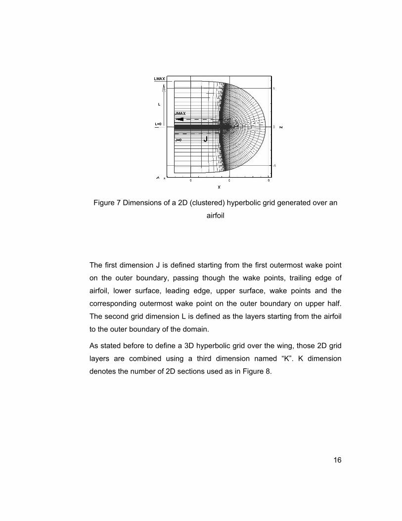
Figure 7 Dimensions of a 2D (clustered) hyperbolic grid generated over an
airfoil
The first dimension J is defined starting from the first outermost wake point
on the outer boundary, passing though the wake points, trailing edge of
airfoil, lower surface, leading edge, upper surface, wake points and the
corresponding outermost wake point on the outer boundary on upper half.
The second grid dimension L is defined as the layers starting from the airfoil
to the outer boundary of the domain.
As stated before to define a 3D hyperbolic grid over the wing, those 2D grid
layers are combined using a third dimension named “K”. K dimension
denotes the number of 2D sections used as in Figure 8.

17
Figure 8 Third dimension K of 3D hyperbolic grid
K dimension proceeds from wing root to wing tip with a clustered formation
focused on wing root and wing tip. When K approaches the wing tip,
perpendicular 2D grid layers are rounded with a number of intermediate
frames called NCIRC as shown in Figure 9 so that a C-O type 3D hyperbolic
grid is formed (Figure 10).

18
Figure 9 Rounding of 2D grid planes at the wing tip

19
Figure 10 A three dimensional C-O type hyperbolic grid

20
CHAPTER 4
FLOW SOLVER
The flow solver used in the wing analysis and design tool is “TAINS_102”
[ref. 28]. TAINS is a multi-block structured Euler/Navier-Stokes finite
difference compressible flow solver developed in Turkish Aerospace
Industries (TAI). The solution of the three-dimensional equations is
implemented by an approximate factorization that allows the system of
equations to be solved in three coupled one-dimensional steps. The most
commonly used method is the Beam and Warming one [ref. 2]. The LU-ADI
factorization [ref. 3] is one of those schemes that simplify inversion works for
the left-hand side operators of the Beam and Warming's. Each ADI operator
is decomposed to the product of the lower and upper bi-diagonal matrices by
using the flux vector splitting technique [ref. 4]. So, because its time
integration is implicit, its solution is accurate and quickly obtained.
Viscosity, turbulence and multi-block properties of TAINS_102 were not
activated in TAIWING thesis study, but they were explained in brief detail for
introductory and preparatory purposes since they were planned to be
included in TAIWING for future work.
For compatibility with TAIWING a few modifications have been made. These
modifications can be categorized into two: flow solver status signalization
and flow solver stopping signalization. The first one, status signalization is
composed of a few lines addition to the flow solver sending current operation
signals to the interface via output channel. Those sent information are used
in informing user about the error if encountered. Another small routine added

21
to the solver is used if residual order drop functionality is activated stopping
the solver when a number written into a signal file is turned from 0 to 1.
Addition of the aforementioned few code lines are also required for
replaceability of solver module. Hence a new flow solver can be replaced
with TAINS_102 with compatibility of output and input files with those
additional routines. TAINS_102 flow solver as in GRID3D grid generator
needs an input file consisting of parameters of flow conditions, solution
methods, grid dimensions and boundary conditions. Those boundary
conditions are generated by TAIWING FORTRAN solver core program
suitable for the provided grid dimensions. Examples to output files of
TAINS_102 are solution result file, residual file and a file containing CL-CD
information.
4.1 Euler/Navier-Stokes Equations and Method of Finite
Differences
Model equations used in computational fluid dynamics are derived from
Navier-Stokes equations. These equations control the motion of an ideal gas
in thermodynamic equilibrium. Derivations of these equations are given in
Appendix B.
4.1.1 Generalized Curvilinear Coordinate Transformations
Generally in computational fluid dynamics, to use equations defined in
cartesian coordinates in physical space i.e. to re-write the equations in
curvilinear coordinates, coordinate transformations from physical space to

22
cartesian space must be applied. Using these transformations, flow domain
around objects with complex geometries can be examined with proper
boundary conditions. In addition, as the same as in flows with shocks flow
regions where flow variables are exposed to high gradients, squeezing of
grid points is possible due to coordinate transformations [ref. 6].
Transformation of Navier-Stokes equations from cartesian space to
curvilinear space are given in Appendix C.
4.1.2 Thin-layer Approach
Viscosity effects in viscous flows with high Reynolds numbers are important
only near the surface and wake regions. Hence for an accurate flow, density
of grid points near surface regions must be increased. When solver is
programmed to solve entire Navier-Stokes equations, derivatives of viscous
terms in flow direction are examined to affect the solution less and in flows
with especially non-separated or mildly separated regions, these terms can
be negligible. Leaving the terms with negligible effects on flow outside
computations increases the speed of solution to a great extent. On the
contrary, full Navier-Stokes equations must be used when dealing with
complex structures since wall curvilinear coordinates tend to change. These
specifications bring us to the Thin-layer approach. Assumptions and details
of Thin-Layer approach are given in Appendix D.
4.1.3 Finite Difference Methods, Numerical Algorithms
With the rapid development in technology of computer speed and memory in
recent years, it became possible to solve approximate form of Navier-Stokes

23
equations in specific orders (boundary-layer, thin-layer N-S, parabolic N-S)
numerically. To develop numerical methods using finite difference method to
solve appearing partial differential equation sets, solving algorithms must be
selected as either explicit or implicit methods. Explicit methods are in
general easier to program and apply. Derivations and applications are
simpler when compared to implicit methods. Implicit methods more-often
have unconditional stability. So it becomes possible to take large steps
through time using implicit methods. Although each iterations last longer,
they converge faster and they use larger time steps in unsteady flows
leading faster solutions compared to explicit ones. They use less memory
due to data structure and above all, solutions are trustworthy since they are
usually convergent.
Derivation of the appropriate numerical algorithm is given in Appendix E.
4.2 Turbulence Models
Development of turbulence models for flows with high Reynolds numbers is
an important aspect in numerical aerodynamic studies. Turbulence factor
must be valued when solving flows around objects as close to reality as
possible.
From most complex to most simple one, statistical turbulence models can be
sorted as: “Reynolds-Stress Transport model”, “Algebraic Stress Modeling”
and “Eddy-Viscosity models”. The last turbulence model in the list, Eddy-
Viscosity models proved useful in solution of numerical aerodynamic
problems up to now. Partial differential equations used in derivation of Eddy-
Viscosity models name these turbulence models as [ref. 18]:

24
2-equation models
1-equation models
1/2-equation models
0-equation models
2-equation and 1-equation models solve two and one differential equations
respectively; whereas 1/2-equation models solve an ordinary differential
equation. No differential equations are solved in 0-equation models and
turbulence effects are represented algebraically. Practically there exists a
large application area for the simplest approach of 0-equation Eddy-
Viscosity models namely, algebraic turbulence models. The main reasons
behind this can be explained by:
1. Simplicity of programming
2. No large time demand in iterated algorithms
3. Separate model definitions in different flow regions
Turbulence models available to TAINS_102 flow solver are Baldwin-Lomax,
K-Omega and K-Epsilon turbulence models.
4.3 Studies of Multi-Block Approach
Main solver and modules creating batch definitions are defined as a library.
Main frame consists of structure of batches. The highest order classification
is the variable named BL which is a subset of all variables of all blocks.
Derived type variables are used everywhere in program, where its data
structure is given in Figure 11.

25
BL
BL(1) BL(2) BL(NBLOCK). . . .
P C D(1:IMAX,1:JMAX,1:KMAX) B(1:NOBC)
JMAX, KMAX, LMAXNoBL,MxNBC,BLKNM, GRDFNAMES,FSMACHRE,ALP,BET,PR,CNBR SMU,DT,INVISC,LAMINILHS ,IRHS,IROE, ISTD..
PARAMETERS CONSTANTS
GAMMA,GAMI,DX1,DY1,DZ1,HD,GD,HDX,HDY,HDZ,RM,PI, RMUE,RK,XT,YT,ZTRINF,UINF,VINF,WINF,EINF,PINF ....
C(3),XY(3,3) Q(ND),S(NV) SVT,TURMU UVW,CN,QQ,RR
SOLUTION AREA
VARIABLES
BOUNDARY
CONDITION
PARAMETERS
IBCTYPE,LB(3,2),NDIRIEXTRP, ITKGV,NoBLC, NoBCC, LOCOPT, UINLET,UOUTLET, ......
CO
FORCE &
MOMENT
FACTORS
CL,CD CF(3) CM(3)
P C D(...) B(1:NOBC)CO
. . . . . . . .. . . . . . . .. . . .
Figure 11 Schematic of program data structure [ref.28]
Although variables in the main program are in this form, to create a multi-
block structure, BL in the sub-structure is avoided from upper variable type
providing simplicity in encoding and letting sub-core solver to send its all
data. So solution of blocks can be processed within the same sub program.
The following example summarizes above statements in terms of commands
and variables:
Example: Solution area parameters of first block in the main program are as
follows:
BL(1)%D0(I,J,K)%Q(1) � Q(1)at the index I,J,Kof first block; namely ρ value
In the sub-programs; namely in SOLVE:

26
D(I,J,K)%Q(1) � Q(1) at the index I,J,K in the block where the main
program executes; namely ρ value
Hence, SOLVE program is called in the main program as follows:
CALL SOLVE( BL(NB)%P0, BL(NB)%C0, BL(NB)%B0, BL(NB)%D0, N)
(NB Block number)
SUBROUTINE SOLVE (P, C, B, D, NCO)
where (P, C, B, D, NCO) short parameter information and all data required
for solution is transferred to SOLVE. On the other hand, SOLVE sub-
program returns one step solution of given block. Here, NCO is the number
of iteration which sends time information to program. Moreover, if this value
is chosen to be negative, the program sends data to the main program
calculating starting values (metrics and boundary conditions to be defined at
the beginning). As can be seen from this structure, all data of all blocks are
usable in the main program. So here it is more suitable for calculations
above blocks. An object that serves this structure becomes clearer here: all
of multi-block structures could be created with command lines in the main
program structure, namely no addition will be required after fully
development of programming in core solver. Data structure in the main
program can be traced in Figure 12 and Figure 13.

27
Figure 12 Tree structure of solver program and module where data structure
is defined [ref.28]

28
Figure 13 Starting definitions forming the last stage of solver main program
[ref.28]

29
Force and moment calculating FOR&MOM should also be considered at this
point. From all block variables there is a classification type variable named
CO which has subsets of CL, CD, CF(3), CM(3) where the first two factors
(as one can guess) are factors of motion and drift of block. CF and CM 3-
component series are force and moment factors in x, y, z coordinates
respectively. FOR&MOM can calculate these factors separately; as a result
total value can be produced with the summation of all block values.
Calculation method of these factors is found by the integration of friction and
pressure forces on surfaces with wall boundary conditions. Also, force and
moment calculations are not in core solver structure but in main structure, so
there is no need for a change in core solver for a change in main program.
4.4 Metric Calculations
Another study to be added to the main structure is metric and Jacobian
calculations. In the new method, after calculation of metrics in each cell, the
average of metrics neighboring that point was taken to find metrics of points.
Metric calculation of a two dimensional example is given in Appendix F.
4.5 Writing Flexible Boundary Conditions Managed From
Input File
Basic approaches in this task are: speed and efficiency to gather results
fast. These conditions are the outcome of the need to use this program as
an aerodynamic analysis tool. The most important point is to leave the core
solver untouched after a specific stage. According to that, boundary

30
conditions are arranged within the same approach. Hence, basic boundary
conditions are specified clearly and use them to create a structure that can
control them using parameters from input file. So, boundary conditions are to
be managed from the input file. Up to now, wall, matching, outlet and
symmetry boundary conditions are created primarily covering most part. In
fact, more boundary conditions other than basic boundary conditions can be
managed externally from the main program. Namely, a lot of boundary
conditions can be derived from these four boundary conditions.
4.5.1 Boundary Conditions Input File
First of all, in account for flexible file location definition, a fixed file called
“INITIAL” points out the name and location of the main input file. That input
file has a higher order language coded structure so it requires command
code definitions. It consists of three main parts (NAMELIST structure of
FORTRAN) in which the first part contains definitions of general parameters
under title (“GENEL”); the second part contains general block parameters
(“BLGENEL”). Physical definitions of flow are given separately for each
block. The parameters in this part can be listed as block numbers, flow
conditions, parameters of time integration, alternative formulae, solution
control parameters and grid dimensions. The third part (“BOCN”) is the
region where boundary conditions are defined one by one where inputs are
classified into two: sets of data: a set consisting of block number, boundary
condition number, boundary condition type and flow region location; and the
other set containing parameters specialized for that boundary conditions. All
parameters are displayed in Table 1. Detailed information about these
parameters is given in the following sections.

31
Table 1 Definitions of input parameters [ref.28]
GENEL
TITLE Project name
NBL, NMAX, NP Block number iteration number and record interval respectively
IREAD, IWRIT Parameters of reading and writing types
BLGENEL
NoBL, MxNBC Block number and maximum boundary condition number
BLKNM, GRDFNAMES Block name and grid filename
FSMACH, RE, ALP,BET, PR Free-stream values (Mach, Reynolds, attack angle, side-slip angle, Prandtl number).
INVISC, LAMIN Inviscid or viscous and Laminar or turbulent selections
CNBR, DT Values related with time integration (Courant number, time step)
ILHS,IRHS, IROE, ISTD,SMU Alternative solution selection parameters
JMAX,KMAX,LMAX,CR,SREF Grid dimensions (Max. number of points in J,K,L index directions, reference location and area
BOCN
IBCTYPE Boundary condition type selection parameter
LB, NDIR Definition of indexes and position and
NoBL, NoBC Block number where the boundary condition belongs to and boundary condition number
IBLOPT, IBLTYPE, UINLET Flow input parameters
UOUTLET Flow output parameters
UWALL,VWALL,WWALL Velocities at wall
IEXTRP, ITKGV, NoBLC, NoBCC, LOCOPT
Matching boundary condition parameters (Interpolation type, transfer definition, block number and boundary condition number of matched boundary condition respectively…)
32
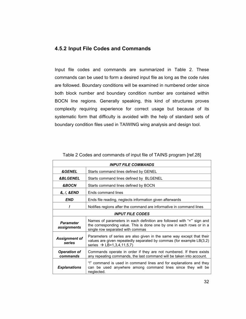
4.5.2 Input File Codes and Commands
Input file codes and commands are summarized in Table 2. These
commands can be used to form a desired input file as long as the code rules
are followed. Boundary conditions will be examined in numbered order since
both block number and boundary condition number are contained within
BOCN line regions. Generally speaking, this kind of structures proves
complexity requiring experience for correct usage but because of its
systematic form that difficulty is avoided with the help of standard sets of
boundary condition files used in TAIWING wing analysis and design tool.
Table 2 Codes and commands of input file of TAINS program [ref.28]
INPUT FILE COMMANDS
&GENEL Starts command lines defined by GENEL
&BLGENEL Starts command lines defined by BLGENEL
&BOCN Starts command lines defined by BOCN
&, /, &END Ends command lines
END Ends file reading, neglects information given afterwards
! Notifies regions after the command are informative in command lines
INPUT FILE CODES
Parameter assignments
Names of parameters in each definition are followed with “=”’ sign and the corresponding value. This is done one by one in each rows or in a single row separated with commas
Assignment of series
Parameters of series are also given in the same way except that their values are given repeatedly separated by commas (for example LB(3,2) series � LB=1,3,4,11,5,7)
Operation of commands
Commands operate in order if they are not numbered. If there exists any repeating commands, the last command will be taken into account.
Explanations “!” command is used in command lines and for explanations and they can be used anywhere among command lines since they will be neglected.

33
Figure 14 An example boundary condition input file [ref.28]

34
4.5.3 Region and Directions Assignments in Boundary
Conditions and Surface Operations
If a boundary condition is to be specified, the region should be defined first
where the boundary condition will be valid. For that reason, a structure is
built using an index form where each region is defined from volume to point.
Figure 15 shows LB series and region definitions.
LB(1,1),LB(2,1),LB(3,1)
J1, K1, L1
LB(1,2),LB(2,2),LB(3,2)J2, K2, L2
Figure 15 Defining systematic regions and designation of LB series values
[ref.28]
The first indices of LB series ξ, η, ζ represent curvilinear surfaces.
LB(1,1)=LB(1,2) � This surface is constant ξ surface.
LB(2,1)=LB(2,2) � This surface is constant η surface.
LB(3,1)=LB(3,2) � This surface is constant ζ surface.

35
LB(2,1)=LB(2,2) & LB(3,1)=LB(3,2)� This represents a ξ line.
LB(1,1)=LB(1,2) & LB(3,1)=LB(3,2)� This represents a η line.
LB(1,1)=LB(1,2) & LB(2,1)=LB(2,2)� This represents a ζ line.
LB(1,1)=LB(1,2) & LB(2,1)=LB(2,2) & LB(3,1)=LB(3,2)� This represents a
point.
If no value matches each other, then that region is a volume.
As stated above, any region can be defined with given LB series. Boundary
conditions are generally defined on surfaces and using double index
representation proves to be useful in most formulations. As an example, on
ξξξξ constant surface η−ζη−ζη−ζη−ζ will be the variables where order plays an important
role. Also, NDIR variable represents the surface direction. If it is positive, the
positive direction will be right direction, otherwise it will be the direction
through decreasing values.

36
Figure 16 Subroutines converting surface definitions to double index form [ref.28]

37
STR and TR subroutines converting surface definitions to double index form
can be found in Figure 16. These subroutines are used as follows:
CALL STR(B(NBC)%LB, B(NBC)%NDIR,KS,MM,NN)
! IMC=1 M Direction is the same with contrary else IMC=2 the inverse to
contrary BC surface
! IMC=0 is not defined yet
DO M=MM(1),MM(2)
DO N=NN(1),NN(2)
CALL TR(KS(0),M,N,0,B(NBC)%LB,J,K,L)
D(J,K,L)%Q(1:NV-1)= ……..
. .
. .
ENDDO
ENDDO
In J, K, L system a transformation to M, N surface system is applied. This
transformation yields simplifications in boundary condition applications.
4.5.4 Wall Boundary Condition
In this type of boundary condition, IBCTYPE is taken as 4. There are two
important aspects in this boundary condition: velocity calculation and
pressure calculation. In fact, pressure calculation is not a direct boundary
condition; energy term in (H.1) is used in boundary condition calculation.
Velocity boundary condition does not pose a problem in Navier-Stokes
solutions because direct velocities are equated to zero. But in Euler

38
solutions velocity boundary condition is more problematic. Velocity boundary
condition is extrapolated by velocities with bearing speed in normal direction
and also perpendicular velocity components are equated to zero. This
approach succeeds in simple models and CO or CH wing type solutions but
it is thought to be problematic in H grid. (Details and equations of boundary
conditions are given in Appendix G).
4.5.5 Symmetry Boundary Condition
IBCTYPE parameter is taken as 8 in this boundary condition. (Details and
equations of boundary conditions are given in Appendix G).
4.5.6 Matching Boundary Condition
Matching is applied whenever two points, axes or planes lie on top of each
other required that they carry exactly the same magnitudes of flow variables.
For example, two grid points at the wing trailing edge both lying on the same
space (although one is defined as on the upper surface and the other one on
the lower surface) are subjected to matching boundary condition to satisfy
Kutta condition.
In this type of boundary condition, IBCTYPE parameter is taken as 5. Until
now, only intersecting type boundary conditions are written so all matched
regions described are one to one matches. When command line near
IBCTYPE=5 line in Figure 14 is considered, some alterations appear in this
boundary condition. Definitions of those are given in Table 3. (Details and
equations of boundary conditions are given in Appendix G).

39
Table 3 Parameters of matching boundary condition [ref.28]
NOBLC Block number of surface to match
NOBCC Boundary condition number in NOBLC block where surface to match is defined
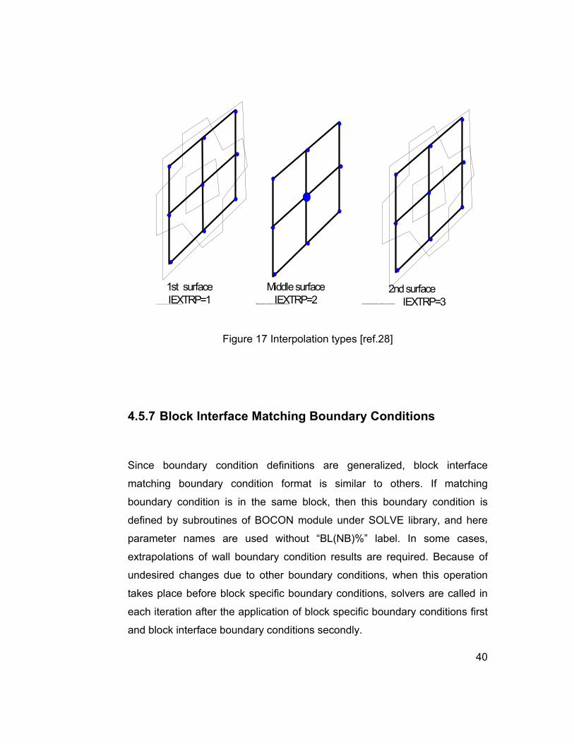
IEXTRP
Extrapolation type 0 � Data transfer only
1 � Interpolation with both surface inners and one point each
2 � Interpolation with both surface inners and 5 points each
3 � Interpolation with both surface inners and 9 points each
Interpolation types are displayed in
Figure 17.
ITKGV
A parameter that specifies active, passive and data transfer of this boundary condition.
0 � Declares that this boundary type is fully passive and defines only regions to the cross boundary condition.
1 � Receives data only from region across.
2 � Receives data from region across and returns calculating cross-value also.
LOCOPT As yet undefined.
40
1st surface IEXTRP=1
Middle surface IEXTRP=2
2nd surface IEXTRP=3
Figure 17 Interpolation types [ref.28]
4.5.7 Block Interface Matching Boundary Conditions
Since boundary condition definitions are generalized, block interface
matching boundary condition format is similar to others. If matching
boundary condition is in the same block, then this boundary condition is
defined by subroutines of BOCON module under SOLVE library, and here
parameter names are used without “BL(NB)%” label. In some cases,
extrapolations of wall boundary condition results are required. Because of
undesired changes due to other boundary conditions, when this operation
takes place before block specific boundary conditions, solvers are called in
each iteration after the application of block specific boundary conditions first
and block interface boundary conditions secondly.

41
4.6 Flexible Boundary Conditions Check in Single-block
Structure
For the first test problem a simple ONERA M6 wing is selected. In Figure 18
results from CO and CH solution grids [ref. 9] are compared and expected
results are found. CH and CO wing grid forms displayed in Figure 21 and in
Figure 22 are the input files used to run TAINS in this form. Results are quite
favorable for this stage but due to singularities in ONERA H grid in Figure
20, solution was not fully concluded.

42
Figure 18 Comparison of pressure distributions of CO and CH wings
controlled by input file using TAINS solver program [ref.28]
ONERA M6 AoA=3.06, 145x34x33 CH and 120x35x24 CO Grid Pressure Distributions
-1
-0.5
0
0.5
1
1.5
-0.2 0 0.2 0.4 0.6 0.8 1 1.2
x/c
-Cp
CH CO 2y/b=0.44 exp.
-1
-0.5
0
0.5
1
1.5
-0.2 0 0.2 0.4 0.6 0.8 1 1.2
x/c
-Cp
CH CO 2y/b=0.9 exp.

43
Figure 19 C-H wing grid (left) and C-O wing grid (right)
(prepared in ICEMCFD) [ref.28]
Figure 20 H grid of Onera M6 wing [ref.28]
a

44
Figure 21 Input file of Onera M6 C-H type wing grid [ref.28]

45
Figure 22 Input file of Onera M6 C-O type wing grid [ref.28]

46
CHAPTER 5
TAIWING FORTRAN SOLVER CORE
This FORTRAN based solver program is the core of TAIWING. The
functionality of it is to manage the discretized flow equations along with the
grid generator and to process output files so that most part of the analysis
function of TAIWING is operated by it. Main algorithm of the FORTRAN
solver core program is given in Figure 23. It starts with reading input file and
checks initial controls before solution launches. The input file contains
parameters of advisor and grid pattern information in addition to information
sent to grid generator and flow solver as shown in Figure 24. Some grid and
solution parameters within input file of TAIWING core program represent
more than a single value called as “multi-valued” parameters. For example,
in addition to the possibility of giving a constant single Mach number as
input, it can be given a set defined with “first value, last value, maximum
number of different values-1” values. Using this property, a series of
solutions can be run as long as parameters are defined as multi-valued
rather than single values.

47
Figure 23 Algorithm of FORTRAN solver core
Reading input file
Initialization routines
Starting Solution series
Preparing grid generator input file
Loading pre-made grids
Launching grid generator
Preparing flow solver input file
Launching flow solver
Error analysis
Processing and saving results
Cleaning workspace
End

48
Figure 24 An example input file of TAIWING FORTRAN solver core

49
Each solution passes through three steps: grid generation, flow solver
solution and process of results. In the first step, either the grid file pointed by
the user is used or the grid is generated with the parameters set by the user.
In the second step, flow solver is run with a provided input file in the suitable
format. In the last step, results of flow solver are compiled, analyzed and all
results are gathered in a single folder within separate sub folders. Waste
files accumulated in the workspace are cleaned with the end of series
solutions and program is reset to its initial state.
The TAIWING FORTRAN solver core program is run automatically at each
analysis startup and permits to be called more than once continuously. Also,
analysis processes after solutions are managed by this program and an
analysis output file is prepared and stored into their relevant folders
containing comparisons of results and experimental data. Analysis files hold
also information about orders of reduction of residuals, CL, CD, aerodynamic
forces and moments gathered after the solutions so that all output files of
flow solver are combined and summarized in each output files providing
solution results to be visualized easily in the graphical user interface.

50
CHAPTER 6
PHYTON INTERFACE
The graphical user interface written in PYTHON script language constitutes
the major part of TAIWING wing analysis and design. PYTHON is an
interpreted, interactive, object-oriented programming language. It is often
compared to TCL, PERL, SCHEME or JAVA [ref. 29]. It combines
remarkable power with very clear syntax. It has modules, classes,
exceptions, very high level dynamic data types, and dynamic typing. There
are interfaces to many system calls and libraries, as well as to various
windowing systems (X11, Motif, Tk, Mac, and MFC). New built-in modules
are easily written in C or C++. PYTHON is also usable as an extension
language for applications that need a programmable interface. The
PYTHON implementation is portable: it runs on many brands of UNIX, on
Windows, OS/2, Mac, Amiga, and many other platforms and it is copyrighted
but freely usable and distributable, even for commercial use. Because of its
open-source nature, it is expanding in every moment due to its modular
expandable structure with the help of users all over the world. Using
PYTHON’s features TAIWING is continuously trying to be extended into
wide application areas like online running protocol over the internet.
PYTHON modules used in the graphical user interface are given in Table 4.

51
Table 4 Modules used in TAIWING PYTHON interface
Time Module used for time control
Os Module used for basic operating system functions
TkMessageBox Module used for operating system specific message box handlings
Sys Module used for operating system commands
Tix Module used for advanced graphical user interface construction
Thread Module used for simplified multi-threads for simultaneous processes
Threading Module used for advanced controls over threads
TkFileDialog Module used for operating system specific file dialog handlings
TkSimpleDialog Module used for operating system specific dialog handlings
TkColorChooser Module used for operating system specific color selection dialog handlings
Shutil Module used for advanced file copying operations
String Module used for functions of string type variables
Math Module used for mathematical functions
Zipfile,Zlib Module used for file compression and decompression
Os.path Module used for advanced files and folders management
Array Module used for operations of series and arrays
Matplotlib.matlab Module used for Matlab style 2D graph operations
PIL Module used for image handlings
Reportlab.pdfgen Module used for PDF report creation
Win32api Module used for Windows platform COM handlings
Win32process Module used for Windows based process management
Win32help Module used for Windows HTML based help file handlings
Win32gui Module used for Windows graphical user interface handlings
Numeric Module used for numerical calculations
OpenGL Module used for open source graphics library handlings for 3D modeling simulation
Winsound Module used for Windows operating system specific sound file handlings

52
TAIWING PYTHON user interface will be described in detail within different
sub-sections, each containing unique functionalities and features. Those
sections used independent of each other in the program together form the
complete user graphical interface.
6.1 Main Window
When TAIWING wing analysis and design program is executed, a loading
screen like Figure 25 appears. Blue area seen on the background is the root
window area where most of other screens are drawn on. TAIWING logo
positioned at the center is displayed for a few seconds in the startup and
performs the file checking of critical files required by the program and
loading configuration file containing program settings. If any critical file is
found to be missing, then program terminates itself followed by an error
message warning the user. Those critical files are listed as flows:
• FORTRAN solver core program executable file
• Grid generator executable file
• Flow solver executable file
Any other missing file except those three critical files like logo image file
does not interrupt the functionality of the program since that kind of errors
are handled silently without user interruption. If no missing critical files exist,
configuration settings are loaded from “Taiwing.ini” file and then loading is
completed leaving user with the main screen. Missing or corrupt
configuration files are replaced with an internal default configuration file with
factory settings.

53
Figure 25 TAIWING program startup screen
Information displayed on the main screen after loading screen is shown in
Figure 26. The buttons shown with detailed information are shortcuts to the
buttons in the main menu bar.

54
Figure 26 Information displayed on TAIWING main screen
6.2 Menus
Figure 27 TAIWING main menu bar
While program is running, the main menu bar stays visible at the top of the
main window as shown in Figure 27. Main menu enables user to switch to
different screens listed. The first button on the main menu is the “New“
button which is used to start a new analysis. When used, it displays another
menu to select further options from, as shown in Figure 28.

55
Figure 28 Menu of options displayed when “NEW” button is used
The first option from this menu, “Create new grid”, directs the user to
“Generating Grid” screen to generate a grid. This way, the user creates a
new grid with given wing geometry and grid dimension parameters and
continues with flow solver modifications. The second option, “Load grid”,
orients the user to “Grid Loading” screen enabling the use of a pre-made
grid in wing analysis. Next option, “Select and use a grid pattern”, demands
selection of a pre-made grid pattern created in “Patterns Manager” screen.
Grid pattern to be selected is used to create a grid suited for the pattern
conditions with wing geometry information acquired later on. Grid pattern in
consideration here is the pure form of a wing grid, non-dimensionalized from
its wing geometry dimensions. Hence it enables generation of the same type
of grid on different wings. The last option in the list, “Use advisor”, handles
the grid generation part automatically without the need of a grid pattern
selection. So, when the user defines the wing geometry, the grid on the
requested wing is generated automatically.
Other buttons on main menu in Figure 27 orients user to “Database
Manager”, “Patterns Manager”, “Advisor”, calculator application of current
operating system, “Options” menu and “Help” screen respectively, which are
discussed separately in proceeding sections. Another frequently used menu
in the program is right click menu containing buttons as shown in Figure 29.

56
Figure 29 Right click menu
6.3 Generating Grid Screen
Figure 30 Generating grid screen

57
Generating grid screen (Figure 30) is the first step in wing analysis
procedure. The purpose of this screen is to get parameters of wing geometry
and grid dimensions from the user and save them. Required parameters are
shown in Figure 31. An explanatory figure is shown on the right side of the
screen for each parameter selected to give a value to. Three of those
parameters (sweep angle, dihedral angle and twist angle) is defined as
multi-valued as in FORTRAN solver core program. To give a single value to
those parameters, (-) signed button near the parameter entry should be
pressed; whereas (+) signed button adds two new entry fields enabling a
series input. First of those multi-valued entry fields is for the first input value
of the parameter; second one is for the last input value of the parameter and
the last entry field is for the total number of elements in the series-1 (or the
step size is calculated as: [last value – first value] / third value). For
example, instead of defining the sweep angle only as 5°, the user may give
5,15,2 values in relevant fields respectively so that sweep angle represents
a series of 5°,10° and 15° angles.
Figure 31 Generating grid screen wing geometry and grid parameters input

58
Another property shown in Figure 31 is to select an airfoil stored in a
database or select an external airfoil using the menu box called “airfoil”.
“Clustering” button activates advanced grid parameters input section (Figure
32). Advanced users can use these additional parameters of clustering
whereas ordinary users may pass this part leaving the values to be set to
defaults by closing the section using “Clustering” button again.
Figure 32 Generating grid screen advanced grid parameters section
As long as a grid is defined in this screen, the user has the option to check
the grid using “Preview” button as in Figure 33 before proceeding further.
Also for detailed examination of the grid, a 3D model of the grid rendered
with OpenGL graphics library is displayed when “Show 3D” button is
pressed. A sample model is shown in Figure 34.

59
Figure 33 Generating grid screen grid preview section
Figure 34 A sample 3D grid model examination

60
Like in other screens, any parameter entry field left blank is filled with
defaults (can be changed in options screen) followed by next screen With
the “Next” button on the lower right corner of the screen, the user proceeds
to the next screen after checks of valid input parameters on the screen and
saving. If an invalid input value is found, (for example if an alpha character is
found in a numerical value entry field or a value out of range is detected) the
user is warned to correct the value by changing background color of the
relevant entry field and warning message displayed on the status bar.
6.4 Solver Parameters Screen
Figure 35 Solver parameters screen

61
Solver parameters screen (Figure 35) is the second step in wing analysis
process after grid generation. The aim of this screen to get flow conditions
information from the user. That information is shown in Figure 36. Each
parameter selected to enter a value shows an informative figure or the
equation of the parameter on the right side of the screen as in generating
grid screen. Two of these parameters (angle of attack and Mach number)
are definable as multi-valued inherited from FORTRAN solver core program.
To give a single value to that parameter (-) signed button is used and
similarly (+) signed button brings two additional entry fields to that parameter
for multi-valued definition. First of those multi-valued entry fields is for the
first input value of the parameter; second one is for the last input value of the
parameter and the last entry field is for the total number of elements in the
series-1 (or the step size is calculated as [last value - first value] / third
value). For example, instead of defining the angle of attack only as 5°, the
user may give 5,15,2 values in relevant fields respectively so that angle of
attack represents a series of 5°, 10° and 15° angles.
Figure 36 Solver parameters screen flow conditions input section

62
“More” button appearing in Figure 36 opens the section where advanced
flow solver modification parameters hide. These parameters (Figure 37) can
be adjusted by advanced users for specification of solution methods to use
whereas ordinary users may pass without any modification by closing the
window, leaving the parameters to their defaults.
Figure 37 Solver parameters screen advanced flow solver modification
section
Like in every other screen, any parameter entry field left blank is filled with
defaults followed by next screen. With the “Next” button on the lower right
corner of the screen, the user proceeds to the next screen after checks of
valid input parameters on the screen and saving. If an invalid input value is
found, (for example if an alpha character is found in a numerical value entry
field or a value out of range is detected) the user is warned to correct the
value by changing background color of the relevant entry field and warning
message displayed on the status bar.

63
6.5 Grid Loading Screen
Figure 38 Loading grid screen
In the beginning of a wing analysis, instead of creating a new grid at the
beginning or enter any grid parameters, the user has the option to load an
existing grid and wing configuration. As shown in Figure 38, all grids stored
in existing databases are listed on the left with an option to export an
external grid file. Selected grid file is displayed in 2D cross-sectional figures
with a summary of grid and wing geometry parameters as shown in Figure
39.

64
Figure 39 Loading grid screen sample grid summary
6.6 Running Screen
After modifications take place in generating grid and solver parameters
screens, last step in wing analysis process comes with running screen.
Running screen is displayed in Figure 40. When running screen is opened,
all solution cases to be solved are listed as in Figure 41. Each solution
enlisted is given a name coded by its key input parameters.

65
Figure 40 Running screen solution startup
Figure 41 Running screen solutions checklist and error status

66
Figure 42 Running screen initialization settings
Before starting to solve all solution cases in the checklist, some settings are
required to be modified from the user as in Figure 42. With the first option
selected as default, the user has the preference to run all solutions by a
specified number of iterations where iteration mechanism is the same as in
flow solver. However the technique of running with a specified length of
iterations has the disadvantage of guessing the right amount of iterations
before launching solver. What TAIWING provides is that, by activating the
second option “Automatic stopper”, residual order controlled automatic
running mechanism is established. The number of order of global residual
subjected to the control mechanism is adjusted via settings screen. The
solver starts with an infinite (~2 billions) number of iterations as input and
when residual order drops that amount, the flow solver is interrupted with a
kill signal sent via the mechanism added to the solver. Residual order drops
are controlled in the same screen as in Figure 43. When specified number of
global residual order drop is reached, flow solver is stopped and process
continues with the next solution case running in the checklist.

67
Figure 43 Running screen global and cl residual tracking
While running of solutions continue in running screen, solution completeness
information and estimation of time left are displayed in the bottom of the
screen as in Figure 44. If the third option “compare with exp. data” in
initialization settings is activated, experimental data files containing wind
tunnel pressure results are required from the user so that maximum and
average errors are calculated with the comparison of solution with
experimental data. The button where time estimation is written on it, is the
pause button pausing and resuming active solutions giving a chance to save
results without waiting for the last iteration to take place. For pausing,
Windows operating system specific application protocol interface process
command are used to interrupt and resume solution threads which seldom
ends up in memory crashes after incorrect rapid usage due to the program’s
complex and fragile structure.

68
Figure 44 Running screen solution status
When running screen is examined in detail, it is seen that a valid input file is
generated for TAIWING FORTRAN solver core program before each
solution or solution series. All information written to that input file consists of
information gathered from the user in grid generating and solver parameters
screen. After preparation of the input file, a thread is created to form a 3 way
pipe connection to TAIWING FORTRAN solver core. First of these
connections is for capturing output material of FORTRAN solver core,
normally directed to monitor output device. The second connection is for
sending keyboard input signals to FORTRAN solver core. The last
connection provides error output messages of FORTRAN solver core and its
sub-connections of flow solver and grid generator to the user interface. The
thread controlling the first pipe connection updates status indicators and
residual graphs continuously. The thread which controls the third error
output connection shows any encountered error messages in errors textbox
shown in Figure 41 and warns the user with messages pointing error source
locations. Errors encountered during solution runs do not interrupt the
procedure since solutions with errors are saved at their last status before
errors occurred. Residual graphs drawn on the screen are auto-scaled,
keeping graph lines in graph regions changing x-y axes. Estimated
remaining time is displayed after calculation of time intervals among initial
iterations and is updated continuously until solution ends. The user is
warned vocally after end of solution runs and guided to the saving solutions
screen for saving desired solutions.

69
6.7 Saving Solutions Screen
Figure 45 Saving solutions screen

70
After end of a solution or a series of solutions, saving of desired solutions is
managed in this screen (Figure 45). Solutions to be saved can be renamed
or examined with their residual graphs again in this screen. Solutions are
saved in folders called “databases” consisting three sub-folders of
“solutions”, “grids” and “airfoils”. More than one database may exist stored in
a computer. Databases are listed in the leftmost list on the screen and
solution contents of the selected database are listed in middle list. The
rightmost list holds completed solutions waiting for the user to save and kept
in a temporary folder.
In truth the definition of a TAIWING database is as follows: a folder under
the name “Databases” is created on program environment folder. This main
folder contains each database folders with their own names where each
database folder consists of three sub folders of solutions, grids and airfoils.
Solutions with their relevant solution files are stacked in solutions folders
numbered from 1 to 9999. Similarly grid files with headers or airfoil
coordinates files are collected in their folders file by file.
Residual graphs of any completed solution are examined using “View
Residuals” button (Figure 46). The next step in wing analysis procedure
continues with the database manager screen after saving solutions.

71
Figure 46 Examination of a new solution’s global (logarithmic scale) and cl
residual graphs in saving solutions screen
6.8 Database Manager
Database manager screen (Figure 47) lists databases stored in computer
and provides tools for examining database sub-sections of solutions, grids
and airfoils. Also, databases are created, renamed, imported and exported
in this screen.

72
Figure 47 Database manager screen solution inspection
Databases to be exported are compressed with zip compression libraries
into a single file with “.tdb” (TAIWING Database) extensions reducing total
disk space coverage by 75%. Using these packed files, databases are
transferred from one computer to another easily. Summary of each selected
solution from the list on the left is shown on the right side of the screen as in
Figure 48. That summary includes wing geometry information used in
solution, dimensions of grid structure, flow conditions, calculated results of
aerodynamic forces and moments and maximum and average errors
measured if any experimental data were provided before solution run. All
this information is gathered form all files of the related solution.
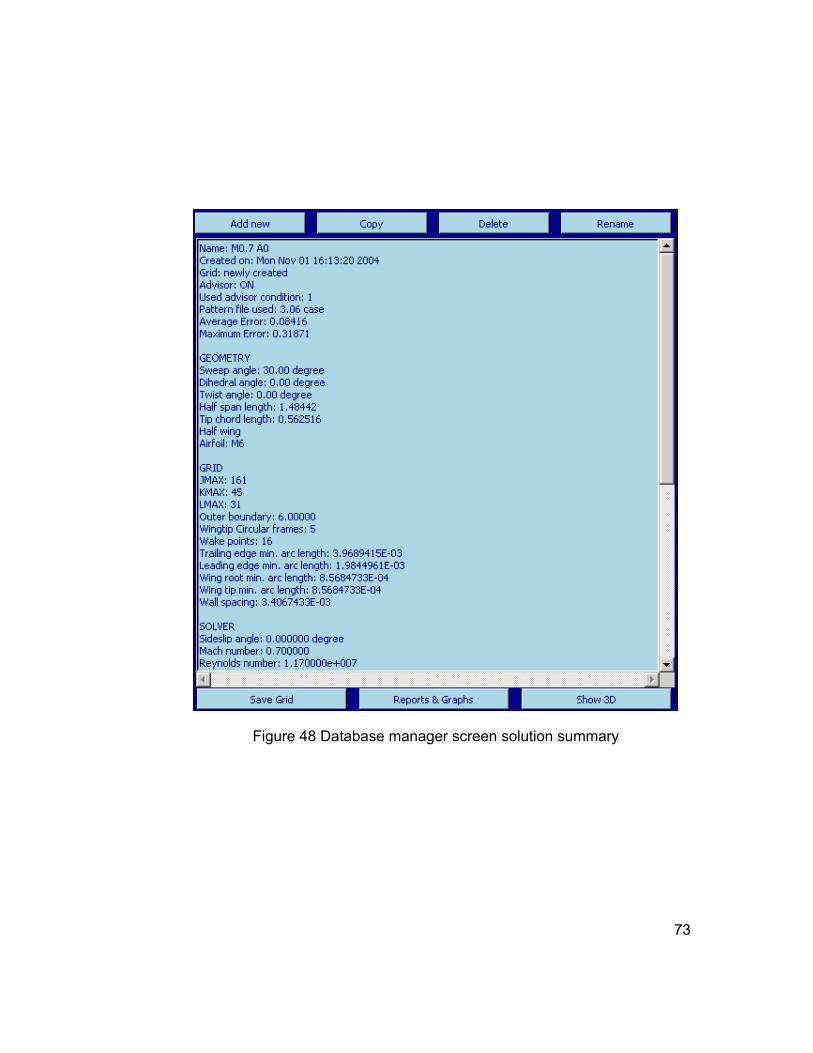
73
Figure 48 Database manager screen solution summary

74
When a grid is selected from a database, its 2D cross-sections are shown as
in Figure 49 to give the user a brief layout of the grid structure. Header files
formed during grid saving process are used during preparations of grid
summaries.
Figure 49 Database manager screen sample grid summary
Lastly, when an airfoil stored in a database is selected, its profile is drawn as
in Figure 50 for brief layout. For that purpose, airfoil coordinates file is used
for airfoil drawing.

75
Figure 50 Database manager screen sample airfoil summary
In addition to the features stated above, database manager screen has
some other features like solution reporting and graph drawing using
“Reports & Graphs” button (Figure 51). Reports & Graphs sub-screen has
the functionality of preparing automatically generated solution reports
(Figure 52), drawing any type of graphs (residuals, contours, x-y plots) at
any wing sections (Figure 53), preparing user-defined multiple-solution
reports (Figure 55) with report wizard (Figure 54) and drawing custom
graphs with multiple solution parameters (Figure 56).

76
Figure 51 Database manager screen reports and graphs wizard
PDF reports generated as in Figure 52 are displayed using an existing PDF
reader application. In these reports, global residual order drop graph is
drawn in logarithmic scale. Below the residual order drop graph, pressure
distribution graphs are drawn, whose wing stations are selected
automatically with suitable values with priority of wing stations where
experimental pressure data files exist. If any experimental data files were
used during solutions, pressure values are compared with blue lines of
calculated data using red dots. Automatic report generation feature is
designed for creation of cumulative archives.

77
Figure 52 Database manager screen automatic PDF solution reporter
sample output

78
Figure 53 Sample output graph generated by database manager screen
custom solution graph generator displaying Cp distribution on a wing root
Figure 54 Database manager screen report wizard for custom PDF report
generation

79
Figure 55 Database manager screen custom PDF report generator sample
output

80
Figure 56 Database manager screen custom graph generator from multiple
solutions
To complete the wing design and analysis tool with post-processing
capabilities, another feature is added to the database manager, enhancing
the program with a graphical solution analyzer. “Show3D” button calls 3D
solution viewer displaying 3D simulation model of selected solution’s field
variables and grid (Figure 57). Grid point coordinates in grid file are drawn in
specified orders to form the grid model using OpenGL based visual
modeling library. The output 3D model is examined using three mouse
buttons each for rotation, zooming and panning (moving model).

81
Figure 57 Database manager screen 3D solution viewer sample solution grid
Field variables at each point are distributed among the 3D modeling field
and combined with colors calculated from their scaled value in a color map
forming flood domain. To increase visibility, flood domain is divided in to 2D
sections of flood fields following the same direction of grid domain. These
cross-sections are controlled with control apparatus on the right hand side of
the screen (Figure 58). The type of flow field variable is selected from a list
in the same control box (density, U velocity, V velocity, W velocity, internal
energy, pressure coefficient and entropy). The output 3D model is again
examined using three mouse buttons each for rotation, zooming and
panning.

82
Figure 58 Database manager screen 3D solution viewer
6.9 Patterns Manager
Another developed feature of TAIWING wing analysis and design tool is the
grid pattern definition. Program has the ability to extract a grid pattern from a
stored grid in a database. This pattern gets selected solution’s grid geometry
information and preserves the same structure by non-dimensionalizing some
of the parameters from grid dimensions. Stored each file containing those
parameters is called a grid pattern file.

83
Figure 59 Patterns manager screen
Each grid pattern file can be used to produce similar grid structures on
different wings. For example, number of wake points in a grid whose pattern
is extracted is the same as the number of wake points in the new grid
produced when that grid pattern is applied to a different wing geometry.
Non-dimensionalization of some parameters from wing geometry information
means dividing geometry variable grid parameters by related wing geometry
dimensions. For example, if a grid has 50 layers along the span of 1.5 meter
length wing, another grid formed using the grid pattern of that grid over a 3
meter length wing will have 100 layers instead of 50, because grid structure
expanded since wing size expanded to preserve the ratio. Using this
property, when a new wing analysis is started, the user will point out a grid
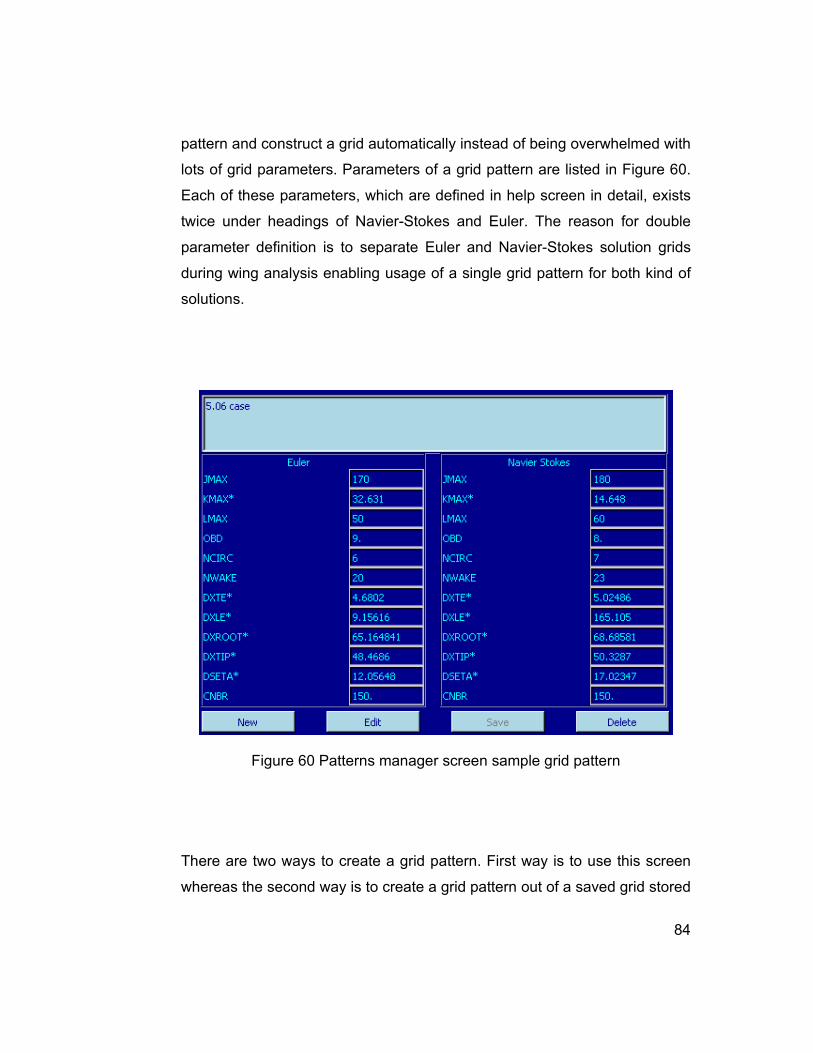
84
pattern and construct a grid automatically instead of being overwhelmed with
lots of grid parameters. Parameters of a grid pattern are listed in Figure 60.
Each of these parameters, which are defined in help screen in detail, exists
twice under headings of Navier-Stokes and Euler. The reason for double
parameter definition is to separate Euler and Navier-Stokes solution grids
during wing analysis enabling usage of a single grid pattern for both kind of
solutions.
Figure 60 Patterns manager screen sample grid pattern
There are two ways to create a grid pattern. First way is to use this screen
whereas the second way is to create a grid pattern out of a saved grid stored

85
in a database. Automatically generated grid patterns require grid pattern
title, Courant number used in the solutions and type of solutions selection
(Euler/Navier-Stokes) from the user. The rest of the pattern is filled
automatically including non-selected flow type parameters. For example if
Euler type was selected, grid pattern parameters for Navier-Stokes flow type
are filled accordingly with increasing grid density on wing surface, etc….
Program stores all grid pattern files in “defaults” folder under main program
folder.
6.10 Advisor
Figure 61 Advisor screen

86
Advisor screen has a similar structure with patterns manager screen as in
Figure 61. TAIWING program proves itself to be “self-improving with more
usage” with the addition of advisor system. Purpose of advisor is to handle
grid generation automatically. So that, in the beginning of a wing analysis, if
“use advisor” option is selected; generating grid screen follows with grid
parameter requirements closed asking only about wing geometry. When the
user, who is not concerned with grid structure, enters flow parameters and
starts solution, advisor criteria are scanned with gathered data of entered
wing geometry and flow parameters to find a suitable criterion pointing to the
related grid pattern so that the grid automatically constructed with that grid
pattern will be used in the current solution. Advisor scanning algorithm works
as in the following example: If an advisor criterion has a Mach number
clause between 0.6 and 1.0 and it points to a grid pattern numbered 3; also
if user defines the Mach number value of his wing analysis solution as a
number between 0.6 and 1.0 and if no other advisor criterion is found, that
criterion will be processed so that grid pattern numbered as 3 will be used to
auto-construct the grid with dimensions specified in the grid pattern file.
Parameters of advisor criteria used in the scanning algorithm are listed in
Figure 62.

87
Figure 62 Advisor screen sample advisor criterion
Advisor criteria are stored in file named “advisor.dat” under main program
folder. If no criteria are found suitable for the flow conditions requested by
user, then the default grid pattern is used. Also, if more than one matching
criteria are found then the one with most specifically detailed clauses among
all will be used. More advisor criteria created with more program usage
leads to better grids and better solution results. This feature also removes
advanced user requirement and renders wing analysis procedures simple
and easy.

88
6.11 Options Screen
Reachable from main menu and its keyboard shortcut, options screen is
formed by three separate tabs. The first tab includes general program
options (Figure 63). Some preferences from this tab are default folder
locations of grid, airfoil, database archives and experimental data files which
provide faster access; contour depth in contoured graphs etc. The second
tab is reserved for colored scheme preferences (Figure 64). The last tab
contains parameter default values encountered in the program interface
which are used whenever relevant entry field of that input parameter is left
blank (Figure 65).
Figure 63 Options screen general program preferences

89
Figure 64 Options screen display preferences
All settings are stored in “taiwing.ini” system initialization file after “OK”
button is pressed and those settings are all acquired and processed at each
startup of the program. In any case when the system file is corrupted,
damaged or lost, the system initialization file is re-constructed with default
settings so program integrity is procured

90
Figure 65 Options screen parameter default value controls
6.12 Help Screen
Help screen, reachable from program help menu is designed on interactive
HTML Web page basis containing TAIWING manual documentation (Figure
66). It has advantages like providing hyperlinks for each parameters,
headings, references etc, providing subject index on the left hand side and
providing a search tool. Help documents is categorized into the following
titles: introduction to program, program structure, detailed information about
each program screens, tutorials, parameters and credits. In addition to the
wide help document given in help screen, help balloon tips are distributed
allover the program for supporting brief helps if cursor is over any object.

91
Figure 66 Help screen
In the first section, program is described briefly with screenshots. In the
second section, detailed structure of the program is given including grid
generator and flow solver used. Third section gives detailed information for
each screen encountered including menus, buttons and properties. The next
section is responsible for educating new users in wing analysis and wing
design processes step by step. Parameters section is reserved for detailed
definition of all parameters used in the program with supporting figures and
web links directly usable within the help screen. The last section gives brief
information about the author of the program and this thesis study.

92
CHAPTER 7
WING DESIGN
In this chapter, wing design capabilities of TAIWING wing analysis and
design tool are demonstrated by choosing a sample wing for validation and
analysis by changing wing geometry, creating charts to compare different
wings to obtain best geometry configuration leading to high lift to drag ratio.
The selected wing [ref. 13] has a uniform Naca0012 airfoil distribution at
6.0x10⁶ Reynolds number providing experimental data at Mach number of
0.5. The wing’s geometry is altered in sweep angle and dihedral angle. The
procedure starts with first validation of analysis results. Secondly, a grid
pattern is created. Thirdly, an advisor criterion is created using the grid
pattern. Then a solution matrix is created and finally results are discussed.
In the first step, suitable grids are constructed manually for the validation of
the wing analysis part of the wing analysis and design tool. After adjusting
the best optimum grid, the results gathered are compared with the
experimental results of pressure values measured on a Naca0012 wing at
0.5 Mach and at 6x10⁶ Reynolds number. In the following two steps,
TAIWING wing and analysis tool is enhanced with advisor criteria to handle
similar wing configurations of Naca0012 type at specified flow conditions,
providing automatic grid generation. Then, a solution matrix is produced with
solutions of varying sweep angle and dihedral. Lastly, using the tools of
TAIWING, several graphs and charts are created and the results were
compared to find the best wing configuration for best lift to drag ratio.

93
7.1 Validation
A Naca0012 wing used for the comparison with experimental data has the
specifications given in Table 5. When given wing dimensions are non-
dimensionalized with respect to the chord length; half span length is found to
be 1.5 units while root and tip chords are equal to 1 unit.
Figure 67 Naca0012 symmetric airfoil

94
Table 5 Naca0012 test wing [ref. 13 ]
Airfoil Naca0012
Sweep angle 20°
Aspect ratio 3
Taper ratio 1
Chord length 10,16 cm
Semispan 15,24 cm
Maximum thickness
1,22 cm
The same wing geometry is constructed in TAIWING wing analysis and
design tool using the wing geometry parameters. Then different grids are
constructed manually on it to obtain a grid fine enough to be able to give
accurate results and coarse enough to decrease computational time
preventing unnecessary calculations. Figure 68 below proves a coarse grid
with JMAX and LMAX dimensions less than adequate.
Figure 68 A coarse grid around test wing with 80x25x18 dimensions

95
Whereas the grid in Figure 69 is a fine grid more than required. Although it
can be used to obtain accurate results, it will slow down the flow solution
process at a great cost of time since each solution iteration is directly
dependent on the number JMAX x KMAX x LMAX. Also it was found that
using too much finer grids near the wing surfaces are not favored by Euler
solutions leading to solver crashes.
Figure 69 A fine grid around test wing with 275x65x80
The grid shown in Figure 70 is suitable for the validation run which is coarse
enough to cover grid domain with grid squares adequate in size and fine
enough to provide accurate solutions. Using this grid TAIWING was run at
the test flow conditions of 6,0x10⁶ Reynolds number, 0,50 Mach number and
angle of attack of 0° and 2°. Each test solution using this grid generally takes
about 55 minutes in a Pentium 4 computer with 3.06 GHz processor speed.
The solution results are given in Figure 71 and Figure 72.

96
Figure 70 A suitable grid around test wing with 200x30x40

97
Figure 71 Solution report of Naca0012 test wing at 0° angle of attack

98
Figure 72 Solution report of Naca0012 test wing at 2° angle of attack

99
The results obtained satisfy the experimental data as can be seen from
pressure residual graphs of 0.25, 0.50 and 0.775 wing stations. In those
graphs, red dots represent wind tunnel test pressure results and the blue
lines represent calculated values. The grid used in these solutions was
selected to be used in grid pattern extraction procedure. Its structure was
preserved while the wing geometry faced changes in sweep angle and
dihedral angle.
7.2 Creating Grid Patterns
In the second step, grid patterns creation was necessary to make use of an
advanced feature of TAIWING wing analysis and design tool: automatic grid
construction. A grid pattern is a file containing dimensionless grid
parameters derived from a grid and used to construct a similar type of grid
on different wing geometries. To create a grid pattern, the grid structure
created in first validation step was used.
Grid pattern creation is an easy task in TAIWING. Firstly, the grid used in
one of the solutions stored in the database was saved using “Save Grid”
button. The following dialog displayed already calculated grid pattern
parameters including non-dimensionalized wing geometry parameters so
there only remained to enter a default file name and Courant number used in
the solutions. The created pattern is shown in Figure 73. Euler part of the
grid pattern file was filled with the grid dimension values and Navier-Stokes
part was calculated with respect to the Euler part with some small alterations
like decrement of wall spacing. “*” sign at the end of some parameters
represent non-dimensionalization of that parameter with respect to the wing
dimensions.

100
Figure 73 Naca0012 test wing grid pattern
7.3 Creating Advisor Criteria
The next stage includes successful definition of an advisor criterion. Advisor
criteria are used in specification of which grid pattern to use due to given
wing geometry and flow conditions information, which enables fully
automatic grid construction. After addition of advisor criteria, the advisor
handles grid generation without question and leaving the user only with input
fields of wing geometry in grid generation screen and flow conditions in
solver screen. For the wing design procedure, an advisor criterion is created
as shown in Figure 74 with a Mach number clause of 0.5, a Reynolds
number clause of 6.0E+6 and an angle of attack clause between 0° and 5°.
Hence any solution done at a 0.5 Mach number and 6.0E+6 Reynolds

101
number with 0° to 5° angle of attack would use the grid pattern file created in
the previous step.
Figure 74 Naca0012 test wing advisor criterion

102
7.4 Preparation of Solution Matrix
The next step, preparation of solution matrix, had the aim of acquiring
solutions with varying sweep and dihedral angles with auto-grid generation
which is validated in the first step. Sweep and dihedral angle input
parameters were arranged in series from 0° to 80° and -5° to 10° with 5°
step length respectively (Table 6.). So multi-valued definitions of (0 – 80 – 8)
and (-5 – 10 – 3) were entered in generating grid screen. Also the wing
geometry is extruded along the span to get 4 units of half-spanned wing to
make the Aspect ratio 8 which is commonly seen in most aircraft wings. The
grid auto-construction mechanism handles this geometry change by
increasing grid layers in K dimension. The angle of attack is adjusted to
5°.The first try outs proved convergence within 1000 iterations so a fixed
iteration interval of 1500 was used for each and all solutions were completed
successfully.
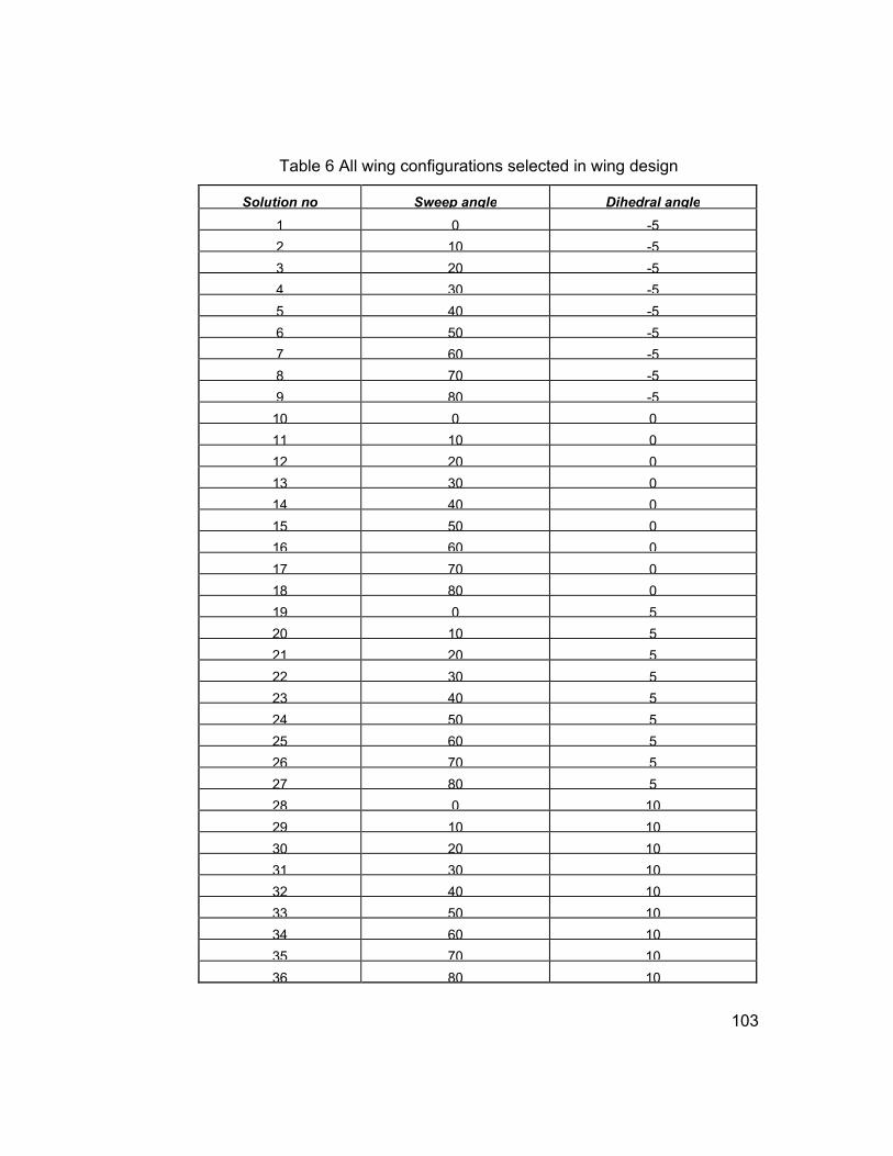
103
Table 6 All wing configurations selected in wing design
Solution no Sweep angle Dihedral angle
1 0 -5
2 10 -5
3 20 -5
4 30 -5
5 40 -5
6 50 -5
7 60 -5
8 70 -5
9 80 -5
10 0 0
11 10 0
12 20 0
13 30 0
14 40 0
15 50 0
16 60 0
17 70 0
18 80 0
19 0 5
20 10 5
21 20 5
22 30 5
23 40 5
24 50 5
25 60 5
26 70 5
27 80 5
28 0 10
29 10 10
30 20 10
31 30 10
32 40 10
33 50 10
34 60 10
35 70 10
36 80 10

104
7.5 Results
After running process of each solution ended, all solutions are recorded in a
TAIWING database. In database manage screen, “Reports & graphs” tool
was launched and all solutions were selected to draw multiple-solution
analysis graphs. These graphs provide any type of graphs of the selected
solutions with chosen graph variables listed. The dynamic list is updated
with only potential variable parameters varying among the selected
solutions. Once two variables are selected, the user is left with the option to
sub-categorize the graph with another variable or group of variables in a
“case” category. For example using this feature, it is possible to draw graphs
of solution result parameters versus sweep angle in groups of different
dihedral angles. Figure 75 demonstrates CL versus sweep angle graph with
different dihedral angle values where selected cases are shown on the right.

105
Figure 75 CL versus sweep angle graph with varying dihedral angles
Figure 75 shows how lift increases slightly as dihedral angle increases but
effect of sweep angle on lift generation is somewhat interesting. Lift
continuously decreases as sweep angle increases with increasing effect.
Dihedral angle can be used to increase lift generation however, more than
10° of dihedral angles are not commonly preferred due to stability
characteristics.

106
Figure 76 CD versus sweep angle graph with varying dihedral angles
Figure 76 proves two things: firstly, drag is inversely proportional to the
sweep angle and it decreases almost linearly as sweep angle is increased;
secondly, dihedral angle slightly increases drag generation similar to its
effect in lift generation. This result is expected since increasing dihedral
angle produces a net effective angle of attack increase resulting in both lift
and drag boost. Drag decrease is an important advantage of using sweep
angle. Figure 77 to Figure 82 displays force and moment coefficients in x, y
and z directions with respect to sweep and dihedral angle changes.

107
Figure 77 CX versus sweep angle graph with varying dihedral angles
Figure 78 CY versus sweep angle graph with varying dihedral angles

108
Figure 79 CZ versus sweep angle graph with varying dihedral angles
Figure 80 MX versus sweep angle graph with varying dihedral angles

109
Figure 81 MY versus sweep angle graph with varying dihedral angles
Figure 82 MZ versus sweep angle graph with varying dihedral angles

110
In figures 75 through 80, X-axis represents roll axis, Y-axis represents pitch
axis and Z-axis represent yaw axis. Conflicting characteristics in those
graphs above 70° sweep angles are due to the over-sweeping of the wing
causing a thin, long wing with greatly altered chord lengths.
In a design process, one of the important aspects of a wing is the lift to drag
ratio (L/D) it has. Table 7 displays the calculated values of lift to drag ratios.
Table 7 Lift to drag ratios with different sweep and dihedral angles
Lift/drag Dihedral
Sweep -5 0 5 10
0 10,75872 10,86903 10,89624 10,84038
10 10,9976 11,08946 11,09683 11,02014
20 11,22065 11,29067 11,27314 11,16915
30 11,37448 11,41827 11,36646 11,22599
40 11,36237 11,36961 11,27591 11,08645
50 10,99833 10,96206 10,8201 10,57888
60 10,02035 9,935094 9,795528 9,458664
70 7,963875 7,847885 7,641973 7,365892
80 4,325409 4,378486 4,367418 4,323468
This analysis shows that at 5° angle of attack, to obtain a higher lift, sweep
should be kept smaller while dihedral angle should be chosen higher; to
obtain a reduced drag, sweep angle should be kept higher whereas dihedral
angle should be chosen smaller. According to Figure 83 sweep angle alone
slowly increases L/D ratio until a critical sweep angle value around 40° and
decreases drastically afterwards while dihedral angle has a net small
decreasing effect over L/D ratio with increasing sweep angle values. As a

111
conclusion, for a Naca0012 wing with 1 unit chord, 4 units of semi-span
length at 6.0E6 Reynolds number, 0.5 Mach number and at 5° angle of
attack, the best design condition providing the highest lift to drag ratio is
obtained at a critical sweep angle of 40° and at 0°dihedral angle. The
dihedral angle can be seen as presenting a positive angle of attack to this
lateral flow, hence generating more lift and drag. But drag increase
dominates the increase in lift generation and it becomes prone to decreased
lift to drag ratio. Increase in lift to drag ratio due to sweep angle is the result
of effective drag reduction but loss of lift in sweep angle is not as linear as
drag reduction so it becomes dominant after a critical sweep angle value. So
sweep angles above this critical value should be chosen wisely especially
for subsonic flows.
L/D versus sweep angle graph
4
5
6
7
8
9
10
11
12
0 10 20 30 40 50 60 70 80
Sweep angle (deg)
Lif
t to
dra
g r
ati
o
Dihedral=-5 Dihedral=0 Dihedral=5 Dihedral=10
Figure 83 Lift to drag ratio versus sweep angle graph with varying dihedral
angles
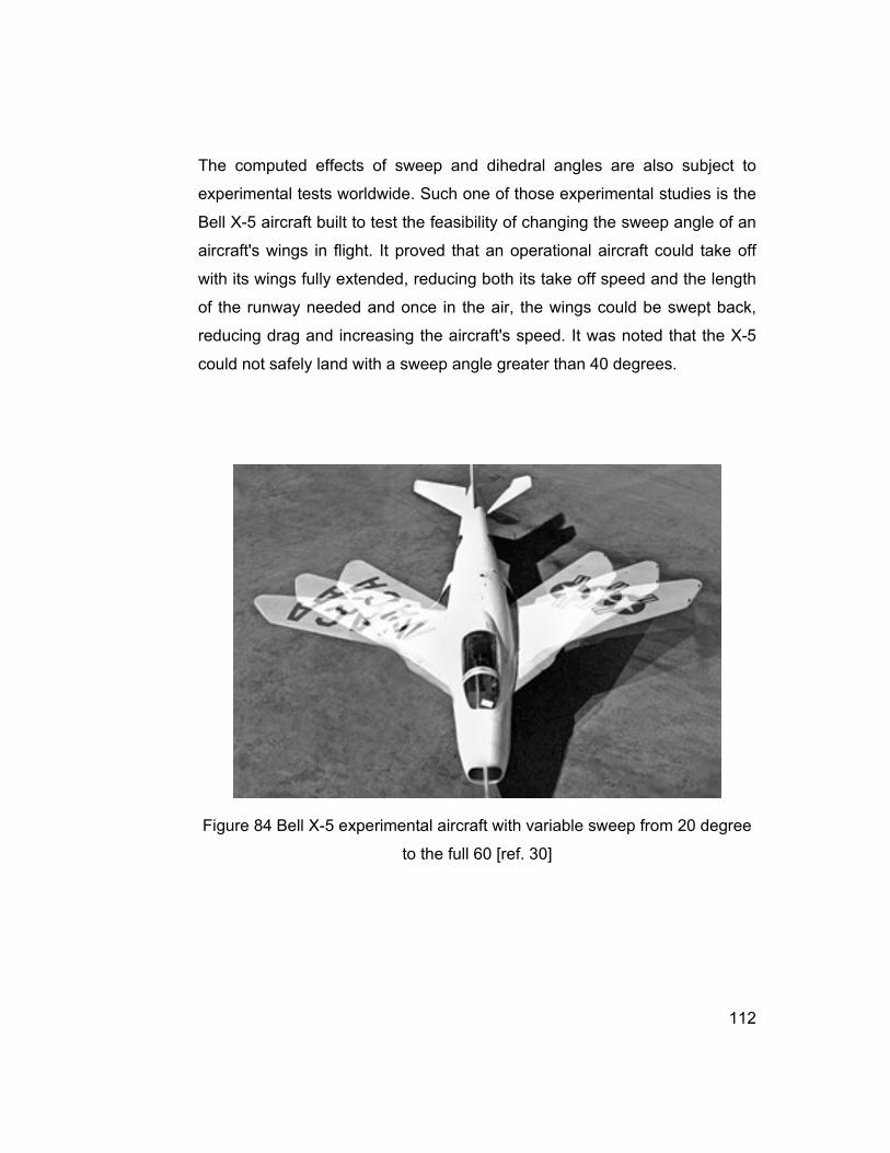
112
The computed effects of sweep and dihedral angles are also subject to
experimental tests worldwide. Such one of those experimental studies is the
Bell X-5 aircraft built to test the feasibility of changing the sweep angle of an
aircraft's wings in flight. It proved that an operational aircraft could take off
with its wings fully extended, reducing both its take off speed and the length
of the runway needed and once in the air, the wings could be swept back,
reducing drag and increasing the aircraft's speed. It was noted that the X-5
could not safely land with a sweep angle greater than 40 degrees.
Figure 84 Bell X-5 experimental aircraft with variable sweep from 20 degree
to the full 60 [ref. 30]

113
CHAPTER 8
CONCLUSION
The scope of this thesis was to develop a computational fluid dynamics
application tool focusing on analysis of wing structures providing rapid
analysis results for use in wing designs. It was aimed to develop a tool which
would optimize time spent and efficiency of wing analyses and design
procedures, and reduce the complexity of an advanced analysis. Developed
wing analysis and design tool contained a graphical user interface
surrounding a FORTRAN solver core consisting of a grid generator and a
flow solver. Several pre-processing and post-processing capabilities were
added enhancing its functionalities like built-in database management
system, automated grid generation, solution report generation, etc.
TAIWING wing analysis and design tool proved to be self-improving with the
addition of an advisor system. Added graphs and reports generators
provided post-processing, cutting-off the need for external post-processing
software. It greatly decreased time required for running a set of solutions
one by one by introducing series-solution generation which had probes of
residual order drop tracking and error handling mechanisms. It also reduced
cost of time and increased efficiency of wing analysis procedures with the
enhanced auto-grid generation feature. It boosted up program handling by
added selective normal/advanced user modes. TAIWING exceeded all the
expectations in functionality with the efficiency of PYTHON script language
used and it proved to be successful enough to show the way to the complete
aircraft analysis and design tool project with the built-in flow solver system.

114
REFERENCES
[1] J. Q. Cordova, T. J. Barth, Grid Generation for General 2-D Regions
Using Hyperbolic Equations, NASA Ames Research Center, January 11-14
1988, AIAA-88-0520, Reno, Nevada
[2] Beam R. M., Warming R. F., “An Implicit Factored Scheme for the
Compressible Navier-Stokes Equations” AIAA Journal, 16, 393, April 1978.
[3]. Fujii K., “Practical Applications of New LU-ADI Scheme for the Three
Dimensional Navier-Stokes Computation of Transonic Viscous Flows”, AIAA
24th Aerospace Sciences Meeting, Reno, Nevada, January 1986.
[4] Steger J. L., Warming R. F., “Flux Vector Splitting of the Inviscid Gas
Dynamics Equations with Application to Finite Difference Methods”, Journal
of Computational Physics, Vol. 40, pp. 263-293, 1981.
[5] Pulliam, T. H., “Euler and Thin-Layer Navier-Stokes Codes: ARC2D,
ARC3D” Computational Fluids Dynamics Workshop Proceedings, UTSI
Publication No. EO2-4005-023-84, Tennessee, March 12-16 1984. The
University Of Tennessee.
[6] Hoffmann, K. A., “Computational Fluid Dynamics for Engineers”,
Engineering Education System, Texas, 1986.
[7] Baldwin, B. S. and Lomax, H., “Thin Layer Approximation And
Algebraic Model For Separated Turbulent Flows”, AIAA paper 78-257 AIAA
16th Aerospace Sciences Meeting, Huntsville, Alabama, 1978.

115
[8] Matsushima, K., Obayashi, S. and Fujii, K., “Navier-Stokes
Computations of Transonic Flows Using the LU-ADI Method”, AIAA paper
87-0421 AIAA 25th Aerospace Sciences Meeting, Reno, Nevada,1987.
[9] Schmitt V. and Charpin F., ”Pressure distribution on the ONERA-M6
Wing at Transonic Mach Numbers”, AGARD AR138, Part B1, 1979
[10] Cebeci, T. and Smith, A. M. O., “Analysis of Turbulent Boundary
Layers”, Academic Press, New York, 1974.
[11] Rumsey, C. L., Taylor, C. L., Thomas, J. L. and Anderson, W. K.,
”Application Of An Upwind Navier-Stokes Code To Two-Dimensional
Transonic Airfoil Flow”, AIAA paper 87-0413 AIAA 25th Aerospace Sciences
Meeting, Reno, Nevada,1987.
[12] Schetz, J. A., “Boundary Layer Analysis”, Prentice Hall, New Jersey,
1993.
[13] Lockman, W.K. and Seegmiller, H.L., “An Experimental Investigation
of the Sub-critical and Supercritical Flow about a Swept Semispan Wing”,
NASA TM-84367, June 1983.
[14] U., Holst, T.L., Cantwell, B.J. and Sorenson, R.L., “Numerical
Simulation of Transonic Separated Flows Over Low Aspect Ratio Wings”,
Journal of Aircraft, Vol. 24, No. 8, pp. 531-539, Aug. 1987.
[15] Vatsa, V.N., “Accurate Solutions for Transonic Viscous Flow Over
Finite Wings”, AIAA-86-1052, Atlanta, GA, 1986.
[16] Abid, R., Vatsa, V.N., Johnson, D.A. and Wedan, B.W., “Prediction of
Separated Transonic Wings”, AIAA-86-1052, Reno, NV, 1986.
[17] Marx, Y.P., “A Practical Implementation of Turbulence Models for the
Computation of Three-Dimensional Separated Flows”, International Journal
for Numerical Methods in Fluids, Vol. 13, pp 775-796, 1991.

116
[18] Rumsey, C.L. and Vatsa, V.N., “A Comparison of the Predictive
Capabilities of Several Turbulence Models Using Upwind and Central-
Difference Computer Codes”, AIAA-93-0192, Reno, NV, 1993.
[19] Menter, F.R., “Zonal Two Equation Turbulence Models for
Aerodynamic Flows”, AIAA-93-2906, Orlando, FL, 1993.
[20] Menter, F.R. and Rumsey, C.L., “Assessment of Two-Equation
Turbulence Models for Transonic Flows”, AIAA-94-2343, Colorado Springs,
CO, 1994.
[21] Obayashi, S. and Fujii, K. “Computation of Three-Dimensional
Viscous Transonic Flows with the LU factored scheme”, AIAA-85-1510,
Cincinnati, OH.
[22] Obayashi, S., Guruswamy, G. and Goorgian, P., “Application of a
Streamwise Upwind Algorithm for Unsteady Transonic Computations Over
Oscillating Wings”, AIAA-90-3103, August 1990, Portland, OR.
[23] Pulliam, T. H. and Chaussee, D.S., “A Diagonal Form of an Implicit
Approximate Factorization Algorithm”, Journal of Computational Physics,
Vol. 39, No. 2, 1981, pp. 347-363.
[24] J. L. Steger and D. S. Chaussee, “Generation of body-fitted
coordinates using hyperbolic partial differential equations”, SIAM Journal on
Scientific and Statistical Computing, 1(4):431-437, 1980.
[25] Marsha J. Berger and Randall J. , "Adaptive Mesh Refinement Using
Wave-Propagation Algorithms for Hyperbolic Systems", SIAM Journal on
Numerical Analysis, Vol. 35, No. 6, 1998, pp. 2298-2316.
[26] Patrick Hanley, Ph.D., “Aerodynamics Software & Strategic
Consulting”, MIT Course XVI G'89, http://www.hanleyinnovations.com/ , last
accessed on 04.01.2006

117
[27] Python Community, “What is Python?”,
http://www.python.org/doc/Summary.html, last accessed on 04.01.2006
[28] Şenol Sergen, Dr. Ali Ruhşen Çete, Yüksel Ortakaya, “Üç Boyutlu
Euler/Navier-Stokes Yapısal ve Yapısal Olmayan Akım Çözücü Geliştirme
Projesi Proje Gelişim Raporu 2003 II. Dönem (Temmuz-Aralık)”, TIDEB
3010088
[29] Python Community, “Python Compared to Other Languages”,
http://python.fyxm.net/doc/Comparisons.html, last accessed on 04.01.2006
[30] Marty Curry, “NASA- NASA Dryden Fact Sheets - X-5”,
http://www.nasa.gov/centers/dryden/news/FactSheets/FS-081-DFRC.html,
last accessed on 08.01.2006

118
APPENDIX - A : 2-D GRID GENERATION
For the grid generation of wing analysis and design tool, the algorithm of
constructing 2D hyperbolic (system of differential equations (A.1.)) grid
generation described below [ref. 1] is used for 2D grids over airfoils at each
cross-section over wing. Hyperbolic grid generation has the advantages of
being orthogonal in two-dimensions, being faster than elliptic systems since
a marching system is used and grid line spacing control by the area or arc
length functions. On the other hand it bears the disadvantages such as: it
can not be used for domains where the outer boundary is specified which is
an ineffective disadvantage for grids around airfoils; boundary discontinuity
may be propagated into the interior domain; undesirable grid system may be
produced if specification of the cell area or arc length functions are not
handled carefully and also there is no possibility to extend to three
dimensions where complete orthogonality exist which is why the grid
generator in this wing and analysis tool uses 2D cross-sections combined to
form 3D.
''' frBrA =+ ης
where
−=
00
00
'
ηη
ηη
xy
yxA ,
−=
00
00
'
ςς
ςς
xy
yxB ,
=
y
xr and
+=
kFFf
0'
(A.1 )

119
In numerical grid generation it is possible to transform a physical domain
around an object which is not definable with equations, to a more complex
but uniform structured computational domain as shown in Figure 85 where
( ) ( )yx,, →ης denotes mapping from computational space to physical space.
Figure 85 Transformation from computational space to physical space)
Such transformation or namely “mapping” is possible with the formulation in
(A.2) where Θ and V representing angle and volume source terms.
These equations form a system of non-linear partial differential equations
and they reduce to the Steger-Chaussee [ref. 24] equations when 0cos =θ .
The solution method for (A.2) will be based upon the following 2x2 system:
θης
ηςcos=
×
rr
rr
Vrr =× ης
where ( )tyxr ,=
( A.2 )

120
The linearization of equations (A.2) is represented by equation (A.3) about
the state x0, y0. Calculation shows that when sinθ≠0, B-1 exists and
Here, λa is the cell aspect ratio. It follows that the eigenvalues of B-1A are ±
λa hence the system below is hyperbolic and the local solution consists of a
right and left running wave.
Initial boundary problem for this set of equations consists of specifying data
on the initial surface (η=0) and the side boundaries (ς=0, ς = ς max). For the
Steger-Chaussee equations ( 0cos =θ ), the boundary curves:
( ) ( )[ ]ηςηςη ,,, yx→ , 0=ς or maxςς = need not intersect the initial curve
fBrAr =+ ης
where
+
−+
−=
00
0
20
00
00
0
20
00 coscos
ης
η
ς
ς
ης
η
ς
ς θθ
rr
y
r
y
rr
x
r
xA ,
+
−+
−=
00
0
20
00
00
0
20
00 coscos
ης
ς
η
η
ης
ς
η
η θθ
rr
y
r
y
rr
x
r
xB ,
( )tVVf 00 ,coscos +−= θθ
(A.3 )
( ) 21det aAB λ−=−
( ) 01 =− ABTr
where ς
ηλ
r
ra =
(A.4)
fBArBr 11 −− =+ ςη
(A.5)
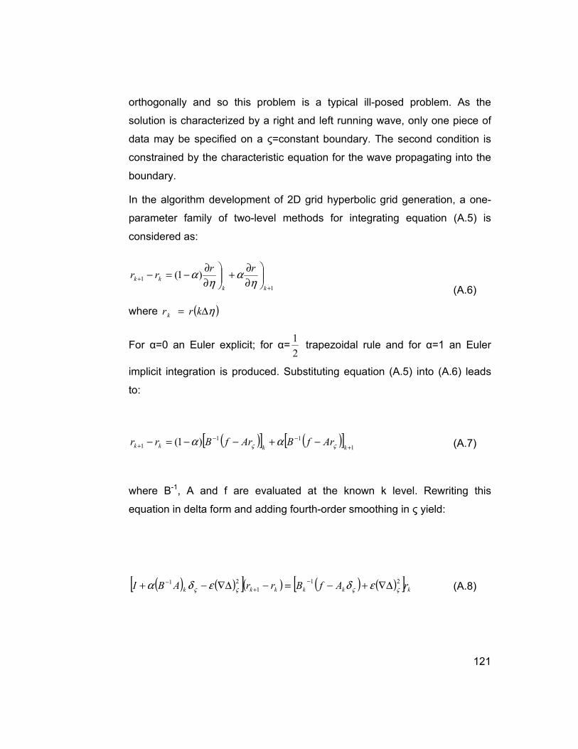
121
orthogonally and so this problem is a typical ill-posed problem. As the
solution is characterized by a right and left running wave, only one piece of
data may be specified on a ς=constant boundary. The second condition is
constrained by the characteristic equation for the wave propagating into the
boundary.
In the algorithm development of 2D grid hyperbolic grid generation, a one-
parameter family of two-level methods for integrating equation (A.5) is
considered as:
For α=0 an Euler explicit; for α=2
1 trapezoidal rule and for α=1 an Euler
implicit integration is produced. Substituting equation (A.5) into (A.6) leads
to:
where B-1, A and f are evaluated at the known k level. Rewriting this
equation in delta form and adding fourth-order smoothing in ς yield:
1
1 )1(+
+
∂
∂+
∂
∂−=−
kk
kk
rrrr
ηα
ηα
where ( )η∆= krr k
(A.6)
( )[ ] ( )[ ]1
11
1 )1(+
−−+ −+−−=−
kkkk ArfBArfBrr ςς αα
(A.7)
( ) ( )[ ]( ) ( ) ( )[ ] kkkkkk rAfBrrABI21
1
21
ςςςς εδεδα ∆∇+−=−∆∇−+−
+−
(A.8)

122
Here ∆∇, and δ are backward, forward and central difference operators in
ς respectively. The differences between this discretization and Steger and
Chaussee are application of delta formation, addition of implicit dissipation
and use of variable integration scheme. These differences enables
smoothing initial discontinuities (increasing ε) and inhibiting grid-shock
formation (setting α>1). As a result bad solutions are avoided by introducing
extra smoothing at the cost of losing orthogonality. This trade-off between
smoothing and orthogonality is acceptable for airfoil geometries.
In addition to providing more local control over grid attributes, the
introduction of an angle source term leads to a well posed initial boundary
value problem. One piece of data may be specified on each side boundary
and these are obtainable from the characteristic relations in theory. However
in practice, the following simpler formulation is employed:
where t) is unit vector tangent to the boundary curve and ⊥∆r is the vector
perpendicular to kk rrr −=∆ +1 and these equations correspond to
specification of slope and extrapolation from the interior respectively. The
computation of source terms is concluded using (A.10) where dr is user
specified normal spacing. Calculating the source terms is thus equivalent to
computing dr and θ.:
0=∆⋅ ⊥rt)
( ) 0int =∆−∆⋅ eriorboundary rrt)
(A.9)
θς sindrrV =
(A.10)

123
APPENDIX - B : EULER/NAVIER-STOKES
EQUATIONS
Starting point of examining 3D compressible, finite and viscous flows with
finite differences method is Navier Stokes equations defined in Cartesian
coordinates in conservative state:
where dependent variables vector of flow q is E, F and G Inviscid flux
vectors which are defined as follows:
Viscous flux vectors on the right hand of equation (B.1) are:
++=+++
z
G
y
F
x
E
z
G
y
F
x
E
t
q vvv
∂∂∂∂
∂∂∂∂
∂∂∂∂
∂∂∂∂
∂∂∂∂
∂∂∂∂
∂∂∂∂
∂∂∂∂
∂∂∂∂
∂∂∂∂
∂∂∂∂
∂∂∂∂
∂∂∂∂
∂∂∂∂
Re
1
(B.1)
( )
( ) ( )
,
, ,
2
2
2
+
+
=
+
+=
+
+
=
=
wpe
pw
wv
wu
w
G
vpe
wv
pv
vu
v
F
upe
wu
vu
pu
u
E
e
w
v
u
q
ρ
ρ
ρ
ρ
ρ
ρ
ρ
ρ
ρ
ρ
ρ
ρ
ρ
ρ
ρ
ρ
(B.2)

124
where
Pressure can be attached to dependent variables using ideal gas relations
as follows:
where γ is the specific heat which is equal to 1.4. “e” is the total energy of
flow in unit volume, ρ is the density, u, v and w are Cartesian velocity
components in x, y and z directions respectively.
−++
=
−++
=
−++
=
zzzzyzx
zz
zy
zx
v
yyzyyyx
yz
yy
yx
v
xxzxyxx
xz
xy
xx
v
qwvu
G
qwvu
F
qwvu
E
τττ
τ
τ
τ
τττ
τ
τ
τ
τττ
τ
τ
τ
0
,
0
,
0
(B.3)
( )
( )
−
+++−=
−
++=
k
kij
i
j
j
iTijij
k
kij
i
j
j
iTij
x
u
x
u
x
up
x
u
x
u
x
u
∂∂∂∂
∂∂∂∂δδδδ
∂∂∂∂
∂∂∂∂
∂∂∂∂
∂∂∂∂µµµµµµµµδδδδσσσσ
∂∂∂∂
∂∂∂∂δδδδ
∂∂∂∂
∂∂∂∂
∂∂∂∂
∂∂∂∂µµµµµµµµττττ
32
32
(B.4)
( ) ( )[ ]222
211 wvuep ++−−= ρρρργγγγ
(B.5)
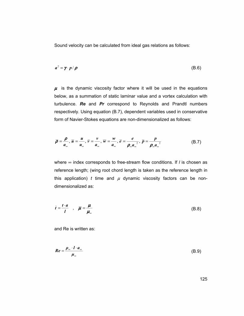
125
Sound velocity can be calculated from ideal gas relations as follows:
µµµµ is the dynamic viscosity factor where it will be used in the equations
below, as a summation of static laminar value and a vortex calculation with
turbulence. Re and Pr correspond to Reynolds and Prandtl numbers
respectively. Using equation (B.7), dependent variables used in conservative
form of Navier-Stokes equations are non-dimensionalized as follows:
where ∞ index corresponds to free-stream flow conditions. If l is chosen as
reference length; (wing root chord length is taken as the reference length in
this application) t time and µ dynamic viscosity factors can be non-
dimensionalized as:
and Re is written as:
ρρρργγγγ /2 pa ⋅=
(B.6)
22,,,,,
∞∞∞∞∞∞∞∞
======a
pp
a
ee
a
ww
a
vv
u
uu
a ρρρρρρρρ
ρρρρρρρρ
(B.7)
∞
=⋅
=µµµµ
µµµµµµµµ,
l
att
(B.8)
∞
∞∞ ⋅⋅=
µ
alρeR
(B.9)

126
In Re number, characteristic velocity is taken as sound speed of free-stream
so depending on free-stream velocity, Re number must be divided by free-
stream Mach number [ref. 5].
Euler equations can be derived from (B.1) and (B.2) by dropping viscous
terms. In other terms, if the right hand side of equation (B.1) is set to zero,
Euler equations are found as:
where dependent variables vector of flow q is E, F and G Inviscid flux
vectors which are defined as follows:
0=+++z
G
y
F
x
E
t
q
∂
∂
∂
∂
∂
∂
∂
∂
(B.10)
( )
( ) ( )
,
, ,
2
2
2
+
+
=
+
+=
+
+
=
=
wpe
pw
wv
wu
w
G
vpe
wv
pv
vu
v
F
upe
wu
vu
pu
u
E
e
w
v
u
q
ρ
ρ
ρ
ρ
ρ
ρ
ρ
ρ
ρ
ρ
ρ
ρ
ρ
ρ
ρ
ρ
(B.11)

127
APPENDIX - C : GENERALIZED CURVILINEAR
COORDINATE TRANSFORMATION
Navier-Stokes equations can be transferred from cartesian space to
curvilinear space using general coordinate transformations:
Solving the equations in curvilinear coordinates in this form (ξ, η ζ ) brings
ease in application of boundary conditions and numerical solution methods.
Transformations are done in curvilinear space by keeping the distance
between each grid point uniform and in unit length. This produces rectilinear
numerical domain of ξ , η and ζ coordinates of uniform grid distribution for
the calculations. Original cartesian space is defined as the physical domain.
Except topological singularity and discontinuity points, each point in physical
domain has a corresponding point in numerical domain. Where singularity
and discontinuities occur, a point with these specifications in physical space
can be represented with more than one point in numerical domain where the
calculations occur [ref. 5]. When a transformation with these properties is
applied, a single code will be will be used in the solution of problems with
multiple geometry and grid systems. Using chain rule, in equality of (B.1)
cartesian partial derivatives can be written in terms of curvilinear coordinates
as follows:
),,,(
),,,(
),,,(
tzyx
tzyx
tzyx
t
ςς
ηη
ξξ
τ
=
=
=
=
(C.1)

128
where ξx, ηx etc. are transformation metrics.
When this transformation is again applied to (B.1), Navier-Stokes equations
can be defined in curvilinear coordinates as in (C.3). Before writing the final
stage of Navier-Stokes equations in curvilinear coordinates, the said
equation derived from finite differences must satisfy the flow at infinity. If this
condition fails, it is clear that a wrong transformation is applied. After
application of the transformations, Navier-Stokes equations in generalized
curvilinear coordinates can be written as follows:
where dependent variables vector and Inviscid flow vector are:
and contravariant velocities are defined as:
( )( )( )
( )( )( )
( )( )( )( )( )
−−−++==
−−−=
−−−=
−−−=
−=
−=
−=
−=
−=
−=
−=
−=
−=
−ξξξξηηηηζζζζζζζζξξξξηηηηηηηηζζζζξξξξξξξξζζζζηηηηηηηηξξξξζζζζζζζζηηηηξξξξ
ττττττττττττ
ττττττττττττ
ττττττττττττ
ηηηηξξξξηηηηξξξξ
ηηηηξξξξηηηηξξξξ
ηηηηξξξξηηηηξξξξ
ζζζζξξξξζζζζξξξξ
ξξξξζζζζζζζζξξξξ
ζζζζξξξξζζζζξξξξ
ζζζζηηηηζζζζηηηη
ζζζζηηηηζζζζηηηη
ηηηηζζζζζζζζηηηη
ζζζζηηηηξξξξ∂∂∂∂
∂∂∂∂
ζζζζζζζζζζζζζζζζ
ηηηηηηηηηηηηηηηη
ξξξξξξξξξξξξξξξξ
ζζζζ
ζζζζ
ζζζζηηηη
ηηηη
ηηηη
ξξξξ
ξξξξ
ξξξξ
zyxzyxzyxzyxzyxzyxzyx
J
zyx
zyx
zyx
xyyxJ
zxxzJ
yzzyJ
yxxyJ
zxzxJ
zyyzJ
xyyxJ
zxxzJ
zyzyJ
zyxt
zyxt
zyxt
z
y
x
z
y
x
z
y
x
,,
,,1
(C.2)
++=+++
ζζζζ∂∂∂∂
∂∂∂∂
ηηηη∂∂∂∂
∂∂∂∂
ξξξξ∂∂∂∂
∂∂∂∂
ζζζζ∂∂∂∂
∂∂∂∂
ηηηη∂∂∂∂
∂∂∂∂
ξξξξ∂∂∂∂
∂∂∂∂
ττττ∂∂∂∂
∂∂∂∂ vvv GFE
eR
GFEq ˆˆˆ1ˆˆˆˆ
(C.3)
( ) ( ) ( )
ˆ ˆ ˆ ˆ 1111
−+
+
+
+
=
−+
+
+
+
=
−+
+
+
+
=
=
pWpe
pWw
pWv
pWu
W
G
pVpe
pVw
pVv
pVu
V
F
pUpe
pUw
pUv
pUu
U
E
e
w
v
v
u
q
t
z
y
x
J
t
z
y
x
J
t
z
y
x
JJ
ζζζζ
ζζζζρρρρ
ζζζζρρρρ
ζζζζρρρρ
ρρρρ
ηηηη
ηηηηρρρρ
ηηηηρρρρ
ηηηηρρρρ
ρρρρ
ξξξξ
ξξξξρρρρ
ξξξξρρρρ
ξξξξρρρρ
ρρρρ
ρρρρ
ρρρρ
ρρρρρρρρ
ρρρρ
(C.4)

129
Flux vectors on the right hand side of the equality are defined as:
It is possible to write the definitions below for viscous flux vector elements:
wvuW
wvuV
wvuU
zyxt
zyxt
zyxt
ζζζζ
ηηηη
ξξξξ
+++=
+++=
+++=
(C.5)
++
++
++
++
=
++
++
++
++
=
++
++
++
++
=
CBA
G
CBA
F
CBA
E
zyx
zzzyzyxzx
zyzyyyxyx
xzzxyyxxx
Jv
zyx
zzzyzyxzx
zyzyyyxyx
xzzxyyxxx
Jv
zyx
zzzyzyxzx
zyzyyyxyx
xzzxyyxxx
Jv
ζζζ
τζτζτζ
τζτζτζ
τζτζτζ
ηηη
τητητη
τητητη
τητητη
ξξξ
τξτξτξ
τξτξτξ
τξτξτξ
0
ˆ
0
ˆ
0
ˆ
1
11
(C.6)
zzzzyzx
yyzyyyx
xxzxyxx
qwvuC
qwvuB
qwvuA
−++=
−++=
−++=
τττ
τττ
τττ
(C.7)

130
APPENDIX - D : THIN LAYER APPROACH
This approach assumes the following statements:
• All surface points must be transformed to constant coordinate plane
(like η = constant coordinate planes).
• Grid density near surface must be in condition to solve viscous flow
effects for a given Reynolds number (at least one or two grid points
must exist in sub-layer.).
• Derivatives of viscous terms will be neglected in ξ direction (in flow
direction) except η direction. All viscous terms will be used.
Although assumptions of thin-layer approach are similar to the ones in
classical boundary layer theory, some basic differences are observed. In
classical boundary layer theory, diffusion processes parallel to surface are
neglected but momentum equation in perpendicular direction to the surface
is swapped with the assumption of equalizing pressure gradients in this
direction to zero. On the other hand, thin-layer approach, in addition to
neglecting diffusion processes parallel to surface, invokes solution of
momentum equations in all directions and hence pressure gradient in normal
direction in boundary layer can be non-zero [ref. 7]. Besides, thin-layer
theory looses its validation in flows with low Reynolds numbers and in
regions with large separations. The flow solver used in this wing analysis
and design tool uses both fully viscous and thin-layer theory calculations.
When thin-layer approach which neglects derivatives of viscous terms in ξ
direction is applied to (C.3) and related equations; Navier-Stokes equations

131
in generalized curvilinear coordinates under influence of thin-layer approach
will be derived [ref. 7] as in form of equation .
where
Terms forming matrix elements can be defined with the equalities in
equation (D.3).
ζζζζ∂∂∂∂
∂∂∂∂
ζζζζ∂∂∂∂
∂∂∂∂
ηηηη∂∂∂∂
∂∂∂∂
ξξξξ∂∂∂∂
∂∂∂∂
ττττ∂∂∂∂
∂∂∂∂ SGFEq ˆ
Re
1ˆˆˆˆ=+++
(D.1)
( )( )( )
( )[ ( ) ( ) ] ( ){ }
+−+
+
+
+
=
−−
−
BCarPA
CwA
CvA
CuA
JS
z
y
x
32112
3
3
3
1
1V5.0
0
ˆ
µµµµζζζζζζζζ
µµµµζζζζ
µµµµζζζζ
µµµµζζζζ
γγγγκκκκµµµµ
ζζζζµµµµ
ζζζζµµµµ
ζζζζµµµµ
(D.2)
=++=
++=++=++=
∞2
2222
222
1V
,
RMwvu
wvuCwvuBA zyxzyxzyx
γγγγκκκκ
ζζζζζζζζζζζζζζζζζζζζζζζζζζζζζζζζζζζζ ζζζζζζζζζζζζ
(D.3)

132
APPENDIX - E : FINITE DIFFERENCES METHOD
Starting point to derivation of used numerical algorithm is the result acquired
by application of implicit time difference equation with three points by Beam
& Warming to thin-layer Navier-Stokes equations given in (D.1) as (E.1).
where n is the time step. Also,
In equation (E.1), E, F, G and S flux vectors are non-linear functions of q
and can be linearized using Taylor series as follows:
The terms in (E.5) are Flux Jacobians and Delta algorithm is obtained
applying (E.3) to(E.1).as in equation (E.5).
( ) 0~
Re~~~~ 11111
=++++∆+−+++ nnnnn SGFEhq ςςηξ
(E.1)
∆=∆=
−=∆ +
thtnqq
qqq
n
nnn
,)(~~
~~~ 1
(E.2)
[ ]
+∆+=
+∆+=
+∆+=
+∆+=
−−+−
+
+
+
)(~~~Re
~Re
)(~~~~)(~~~~)(~~~~
21111
21
21
21
hOqMJSS
hOqCGG
hOqBFF
hOqAEE
nnnn
nnnn
nnnn
nnnn
(E.3)

133
Partial space derivatives obtained from the formulation will be estimated with
second-degree central differences. Hence the algorithm has first order
sensitivity in time and second order sensitivity in space.
“Approximate Factorization” is applied in equation (E.5) to simplify numerical
calculations. Afterwards numerical algorithm is developed using “LU-ADI”
[ref. 8]. Also to satisfy stability during solution of numerical method
especially in non-linear flows (like flows with shocks), artificial dissipation
terms are added to the algorithm.
q
SM
q
GC
q
FB
q
EA ~
~~
,~
~~
,~
~~
,~
~~
∂
∂=
∂
∂=
∂
∂=
∂
∂=
(E.4)
[ ][ ]nnnn
nnnnn
SGhFhEhh
qMhJChBhAhI
~Re
~~~
~~Re
~~~
1
11
ςςηξ
ςςηξ
∂−∂+∂+∂−
=∆∂−∂+∂+∂+
−
−−
Λ
(E.5)

134
APPENDIX - F : METRIC CALCULATIONS
A two-dimensional example will clear out the difference as follows. Metric
calculation of a 2D cell configuration shown in Figure 86 is given in (F.1).
1 2
3 4
(I-1,J+1) (I,J+1) (I+1,J+1)
(I-1,J) (I,J)(I+1,J)
(I+1,J-1)(I,J-1)(I-1,J-1)
Figure 86 Example 2D cell configuration

135
4/)(),(
2
)1,1()1,(
2
),1(),(
2
)1,()1,1(
2
),(),1(
2
),1(),(
2
)1,1()1,(
2
),(),1(
2
)1,()1,1(
2
)1,1()1,1(
2
)1,1()1,1(),(
4321
4
3
2
1
ξξξξξ
ξ
ξ
ξ
ξ
ξ
xxxxJIx
JIxJIxJIxJIxx
JIxJIxJIxJIxx
JIxJIxJIxJIxx
JIxJIxJIxJIxx
methodnew
JIxJIxJIxJIxJIx
methodold
+++=
−++−
−++
=
−+−−
−+−
=
++
−++++
=
+−
−+++−
=
−−+−+
−+−+++
=
(F.1)

136
APPENDIX - G : BOUNDARY CONDITIONS
Wall Boundary Condition
p
q
e
Pp :tangent vector in p directionPq :tangent vector in q directione : Surface normal vector
O
r
Figure 87 Vector representations on grid surfaces
( )222
2
1
1wvu
pe +++
−= ρρρρ
γγγγ
(G.1)

137
where p, q, r � ξ, η, ζ or η, ζ, ξ or ζ, ξ, η representation is made. Using
equations (G.2) and (G.3), Euler wall boundary conditions can be written as
follows:
Calculations of wall velocity boundary condition for r constant surface;
Extrapolated from velocities in P, Q, r direction, and R is set to zero.
Transformation is applied from P, Q, R tangent velocities to u, v and w
Cartesian velocities.
Wall pressure calculation (for r constant surface);
Normal momentum equation can be written as in equation (G.4).
[ ] [ ]
[ ]
surface of velocity Normal;
directionr in locity tangent ve; R
direction qin locity tangent ve;
direction pin locity tangent ve;
1
)(
,,
2222
zyxn
rrr
qqq
ppp
zyx
zyxqp
qp
qqqqpppp
eweveuV
zwyvxu
zwyvxuQ
zwyvxuP
rrrrrrPP
PPe
zyxPzyxP
⋅+⋅+⋅=
⋅+⋅+⋅=
⋅+⋅+⋅=
⋅+⋅+⋅=
++=
×
×=
==
(G.2)
zzz
yyy
xxx
rRqQpPw
rRqQpPv
rRqQpPu
⋅+⋅+⋅=
⋅+⋅+⋅=
⋅+⋅+⋅=
cartesian o tangent tfrom s velocitieoftion Transforma
(G.3)

138
where P is pressure. Equation (G.4) can be written in simpler form as
follows:
As a result, formulation is converted to Approximate Factorization with
equations below and consecutive closed solution with pressure solutions are
obtained in two directions.
Although better results are obtained when the program uses this method in
pressure calculations, application difficulties rose in complex cases. On top
of that extrapolation from practical top points was tried, these two methods
were compared in solutions for testing purposes and it was decided to use
extrapolation method due to insignificant differences and practical usage.
( ) ( )222
222222
zyx
qzqyqxpzpypx
rq
zyx
zzyyxx
p
zyx
zzyyxx
rrr
wrvrurQwrvrurP
PPrrr
rqrqrqP
rrr
rprprp
++
⋅+⋅+⋅+⋅+⋅+⋅−
=′+′
++
⋅+⋅+⋅+′
++
⋅+⋅+⋅
ρρρρρρρρΛΛ
(G.4)
)1(ˆ,,
ˆ)(ˆ
)1()(
))()1((
1111
21
21
21
21
+′+∆⋅−=∆⋅=∆⋅=
=′+′⋅−′⋅−
+′−∆⋅=′−′⋅∆⋅+′⋅∆⋅
=∆
′−+′+′⋅+′⋅
=′+′⋅+′⋅
rPrRRrDDrDDwhere
RrPPDPD
rPrRrPPrDPrD
Rr
rPrPPDPD
RPPDPD
qp
qp
qp
rqp
))
)
(G.5)
RrPDIDI qpˆ)()ˆ()ˆ( 21 ≅′⋅−⋅− δδδδδδδδ
(G.6)
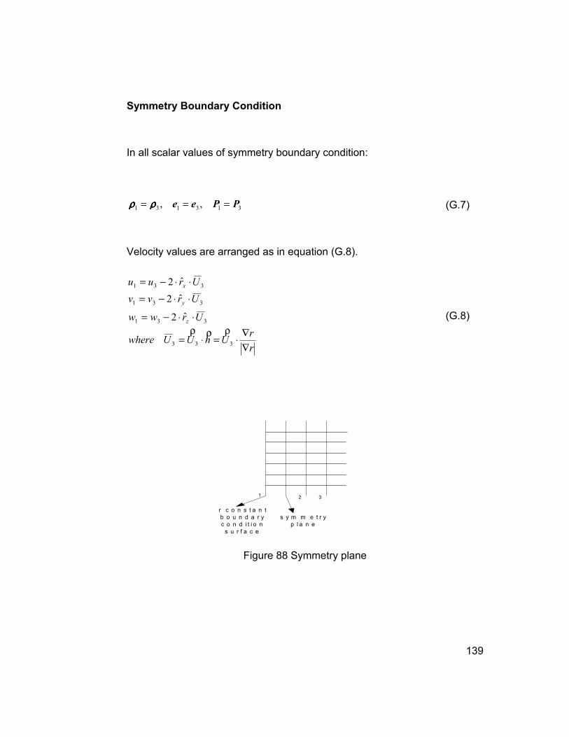
139
Symmetry Boundary Condition
In all scalar values of symmetry boundary condition:
Velocity values are arranged as in equation (G.8).
s y m m e t r yp l a n e
r c o n s t a n tb o u n d a r yc o n d i t i o ns u r f a c e
1 2 3
Figure 88 Symmetry plane
313131 ,, PPee === ρρρρρρρρ
(G.7)
r
rUnUUwhere
Urww
Urvv
Uruu
z
y
x
∇
∇⋅=⋅=
⋅⋅−=
⋅⋅−=
⋅⋅−=
333
331
331
331
ˆ2
ˆ2
ˆ2
ρρρ
(G.8)

140
Matching Boundary Condition
Inverse distance method is used between these points for interpolation.
Interpolation formulation of inverse distance method with m points is given in
equation (G.9).
∑
∑
=
=
⋅
=⇒=m
n
n
m
n
nn
i
BAf
BgBAf
AgBA
BAf
1
1
),(
)(),(
)(1
),(αααα
(G.9)

![ON THE NAVIER-STOKES EQUATIONS WITH ...and has been discussed even for the classical Navier-Stokes and Euler equations by many authors (see Duchon and Robert [4], Eyink [6], and Nagasawa](https://img.dokumen.tips/doc/110x75/6119d5f03342476b621f6420/on-the-navier-stokes-equations-with-and-has-been-discussed-even-for-the-classical.jpg)


