Embed Size (px)
Citation preview

Working Reports contain information on work in progress
or pending completion.
The conclusions and viewpoints presented in the report
are those of author(s) and do not necessarily
coincide with those of Posiva.
Lee Hartley, Peter Appleyard
Steven Baxter, Jaap Hoek
David Roberts, David Swan
Serco
Working Report 2012-32
Development of a Hydrogeological DiscreteFracture Network Model for the Olkiluoto Site
Descriptive Model 2011Volume II
Base maps: ©National Land Survey, permission 41/MML/12


247
13 ELABORATED DFN - SITE-SCALE CONFIRMATORY TESTS
This section details a number of confirmatory tests against different sorts of site data for models based on the Elaborated Hydro-DFN description. Fracture networks are developed from the Chapter 10 definition, and for both DFN and ECPM models as appropriate to the confirmatory test considered. Site-scale DFN models are similar to those defined in Chapter 12, and further details on their development are presented in Section 12.2. For all confirmatory tests, a minimum stochastic fracture radius of 8.26m (equivalent to a side length of 15m) was applied throughout the domain, with smaller fractures local to the repository neglected.
Confirmatory analyses for the Hydro-DFN models involve comparison with baseline head measurements /Ahokas et al. 2008/, pumping tests /Löfman et al. 2009/, /Vaittinen et al. 2008/ and hydrochemistry /Partamies and Pitkänen 2012/. Calibration of model predictions yield minor changes to transmissivities in both hydrozones and background fractures. Multiple realisations of the stochastically generated fracture networks using Case A, Case B and Case C fracture size models are considered with semi-correlated transmissivity distributions used throughout.
As for the Phase I analysis in Chapter 7, the Elaborated Hydro-DFN is upscaled to create an equivalent continuum porous medium (ECPM) site-scale model. Using this ECPM model, a suite of palaeohydrogeological calculations are performed, examining the evolution of the chemical composition of groundwaters and provide confirmatory analysis with present-day measurements. In addition, sensitivities of groundwater head and chemical composition to model parameters are assessed through a selection of model variants, and uncertainties analyzed by considering multiple realisations of the ECPM model. Finally, the effects of incorporating the transmissivity adjustments defined from the baseline head and pumping test calibrations are also examined.
13.1 Baseline heads
Measurements of groundwater levels are available from long-term monitoring in a number of open drillholes at Olkiluoto using multi-packers and flow logging techniques. However, these groundwater head measurements exhibit natural variations with time due to the seasonal fluctuations of the groundwater table on the island. Baseline heads reported in /Ahokas et al. 2008/ correspond to fresh water heads; taking into account the increasing salinity of groundwater with depth and are corrected to a long-term average of the groundwater table.
Confirmatory tests against baseline heads in a selection of drillholes are performed, by solving fresh water, site-scale Hydro-DFN models. The effects of increasing salinity of groundwater with depth are thus neglected in the Hydro-DFN models, and as such, calculated drillhole pressures are only representative of the measured baseline heads down to elevations around –400 m (see Figure 3-5). To form tractable simulations, the full site-scale models are constrained between coordinates (1524576, 6791281) and (1526976, 6793660); selected based on suitable distances from all monitoring drillholes, and the shoreline of Olkiluoto Island. The depth of the model is truncated at –800 m. A zero head boundary condition is specified at the lateral boundaries of the domain and across the top of the model for the sea bed. Otherwise an infiltration rate is applied to
248
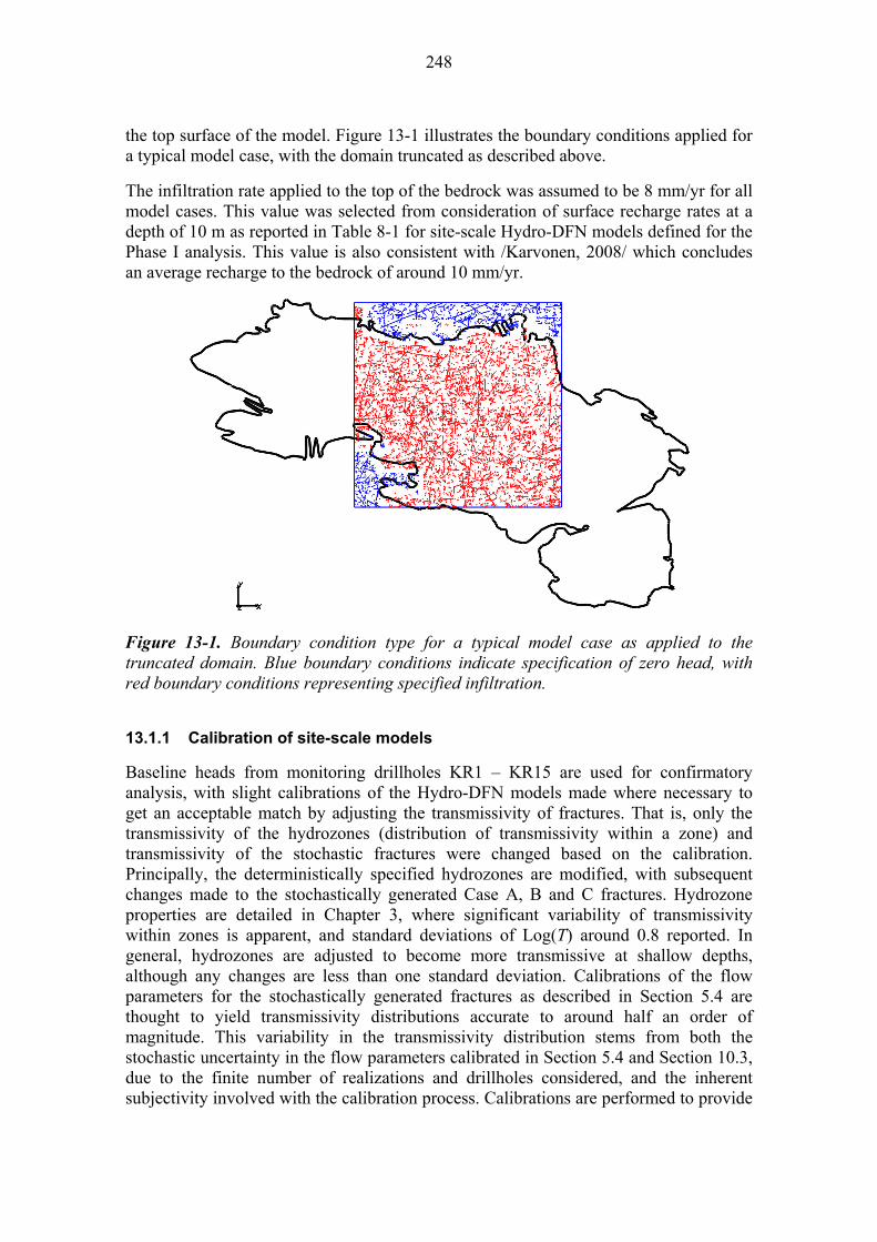
the top surface of the model. Figure 13-1 illustrates the boundary conditions applied for a typical model case, with the domain truncated as described above.
The infiltration rate applied to the top of the bedrock was assumed to be 8 mm/yr for all model cases. This value was selected from consideration of surface recharge rates at a depth of 10 m as reported in Table 8-1 for site-scale Hydro-DFN models defined for the Phase I analysis. This value is also consistent with /Karvonen, 2008/ which concludes an average recharge to the bedrock of around 10 mm/yr.
Figure 13-1. Boundary condition type for a typical model case as applied to the truncated domain. Blue boundary conditions indicate specification of zero head, with red boundary conditions representing specified infiltration.
13.1.1 Calibration of site-scale models
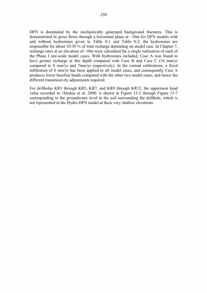
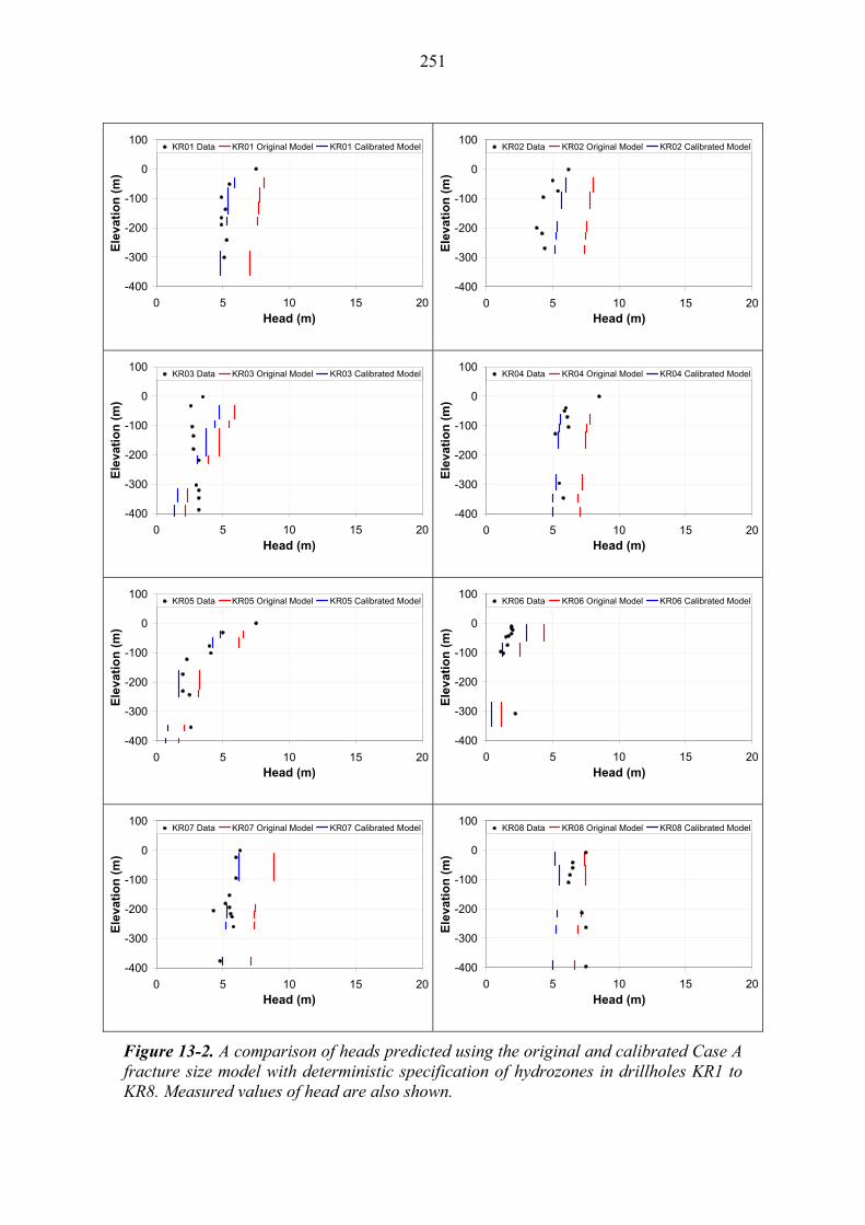
Baseline heads from monitoring drillholes KR1 – KR15 are used for confirmatory analysis, with slight calibrations of the Hydro-DFN models made where necessary to get an acceptable match by adjusting the transmissivity of fractures. That is, only the transmissivity of the hydrozones (distribution of transmissivity within a zone) and transmissivity of the stochastic fractures were changed based on the calibration. Principally, the deterministically specified hydrozones are modified, with subsequent changes made to the stochastically generated Case A, B and C fractures. Hydrozone properties are detailed in Chapter 3, where significant variability of transmissivity within zones is apparent, and standard deviations of Log(T) around 0.8 reported. In general, hydrozones are adjusted to become more transmissive at shallow depths, although any changes are less than one standard deviation. Calibrations of the flow parameters for the stochastically generated fractures as described in Section 5.4 are thought to yield transmissivity distributions accurate to around half an order of magnitude. This variability in the transmissivity distribution stems from both the stochastic uncertainty in the flow parameters calibrated in Section 5.4 and Section 10.3, due to the finite number of realizations and drillholes considered, and the inherent subjectivity involved with the calibration process. Calibrations are performed to provide

249
a best match with the baseline heads recorded in the monitoring drillholes KR1 – KR15 as detailed in /Ahokas et al. 2008/.
Subsequent to this analysis, several realisations of the Hydro-DFN for Case A, B and C intensity-size models, along with heterogeneous hydrozone transmissivities are considered.
13.1.2 Calibrated predictions of baseline heads
The first confirmatory test was to consider the predicted heads within several drillholes using a DFN model, and consider potential changes to fracture transmissivities necessary, if any. Using a single realisation of the stochastically generated Case A, B and C fractures, with deterministically specified hydrozones, site-scale Hydro-DFN models are calibrated using baseline heads in monitoring drillholes KR1 – KR15. Sections of drillhole modelled are based on packer locations described in /Ahokas et al. 2008/, are used to obtain the measured values. However, to ensure sufficient likelihood that random fractures intersect with a given drillhole test section, packer locations are extended such that a minimum of 25m drillhole length is considered. For cases where measurements were determined from flow logging techniques, and recorded at specific depths within a drillhole, suitable drillhole test sections were defined.
Calibrations initially focused on changes to the hydrozone transmissivities used for each of the intensity-size cases A, B and C. Optimal changes are detailed in Table 13-1 with subsequent modifications to the stochastically generated fractures also recorded.
Table 13-1. Transmissivity adjustments determined from site-scale calibrations using baseline head measurements in drillholes KR1 to KR15. The transmissivity values are changed in all fractures in the sets/domains indicated by the adjustment factors given.
Fracture Classification
Calibration Details
Domain Depth Orientation Transmissivity adjustment
Hydrozones All
z ≥ –150
All
T × 4
–150 > z ≥ –400 T × 3
z < –400 T × 2
Case A All Depth Zone 1 SubV T / 2
Case B All Depth Zone 1 All T × 3
Case C All Depth Zone 1 All T × 2
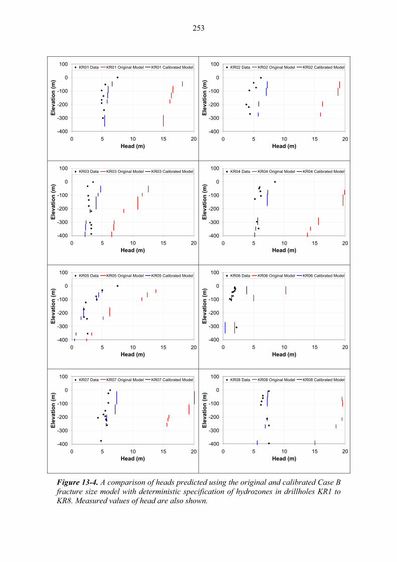
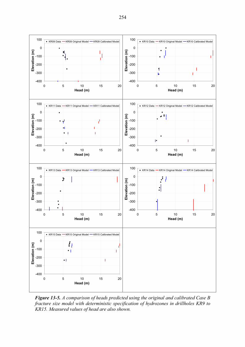
Figure 13-2 through Figure 13-7 illustrate results for monitoring drillhole for each of the unmodified and calibrated model cases A, B and C. Transmissivities of the hydrozones and corresponding fracture model are adjusted as outlined in Table 13-1. For random fractures generated from Case B and Case C fracture size models, transmissivities are increased for all fractures within Depth zone 1, whereas for Case A fractures, transmissivities are reduced only for E-W and N-S sets at this depth. These adjustments to the transmissivities are within the bounds of uncertainty with which it is considered the Hydro-DFN parameters can typically be determined, about a factor 2-3.
Within the models, hydrozones have limited extent, and few are found to extend to the top of the domain. As such, infiltration across the top surface of the site-scale Hydro-
250
DFN is dominated by the stochastically generated background fractures. This is demonstrated in gross flows through a horizontal plane at –10m for DFN models with and without hydrozones given in Table 8-1 and Table 8-2; the hydrozones are responsible for about 10-30 % of total recharge depending on model case. In Chapter 7, recharge rates at an elevation of -10m were calculated for a single realisation of each of the Phase I site-scale model cases. With hydrozones included, Case A was found to have greater recharge at this depth compared with Case B and Case C (16 mm/yr compared to 8 mm/yr and 7mm/yr respectively). In the current calibrations, a fixed infiltration of 8 mm/yr has been applied to all model cases, and consequently Case A produces lower baseline heads compared with the other two model cases, and hence the different transmissivity adjustments required.
For drillholes KR1 through KR5, KR7, and KR9 through KR12, the uppermost head value recorded in /Ahokas et al. 2008/ is shown in Figure 13-2 through Figure 13-7 corresponding to the groundwater level in the soil surrounding the drillhole, which is not represented in the Hydro-DFN model at these very shallow elevations.
251
-400
-300
-200
-100
0
100
0 5 10 15 20Head (m)
Ele
vati
on
(m
)
KR01 Data KR01 Original Model KR01 Calibrated Model
-400
-300
-200
-100
0
100
0 5 10 15 20Head (m)
Ele
vati
on
(m
)
KR02 Data KR02 Original Model KR02 Calibrated Model
-400
-300
-200
-100
0
100
0 5 10 15 20Head (m)
Ele
vati
on
(m
)
KR03 Data KR03 Original Model KR03 Calibrated Model
-400
-300
-200
-100
0
100
0 5 10 15 20Head (m)
Ele
vati
on
(m
)
KR04 Data KR04 Original Model KR04 Calibrated Model
-400
-300
-200
-100
0
100
0 5 10 15 20Head (m)
Ele
vati
on
(m
)
KR05 Data KR05 Original Model KR05 Calibrated Model
-400
-300
-200
-100
0
100
0 5 10 15 20Head (m)
Ele
vat
ion
(m
)
KR06 Data KR06 Original Model KR06 Calibrated Model
-400
-300
-200
-100
0
100
0 5 10 15 20Head (m)
Ele
vati
on
(m
)
KR07 Data KR07 Original Model KR07 Calibrated Model
-400
-300
-200
-100
0
100
0 5 10 15 20Head (m)
Ele
vati
on
(m
)
KR08 Data KR08 Original Model KR08 Calibrated Model
Figure 13-2. A comparison of heads predicted using the original and calibrated Case A fracture size model with deterministic specification of hydrozones in drillholes KR1 to KR8. Measured values of head are also shown.
252
-400
-300
-200
-100
0
100
0 5 10 15 20Head (m)
Ele
vati
on
(m
)
KR09 Data KR09 Original Model KR09 Calibrated Model
-400
-300
-200
-100
0
100
0 5 10 15 20Head (m)
Ele
vati
on
(m
)
KR10 Data KR10 Original Model KR10 Calibrated Model
-400
-300
-200
-100
0
100
0 5 10 15 20Head (m)
Ele
vati
on
(m
)
KR11 Data KR11 Original Model KR11 Calibrated Model
-400
-300
-200
-100
0
100
0 5 10 15 20Head (m)
Ele
vati
on
(m
)
KR12 Data KR12 Original Model KR12 Calibrated Model
-400
-300
-200
-100
0
100
0 5 10 15 20Head (m)
Ele
vati
on
(m
)
KR13 Data KR13 Original Model KR13 Calibrated Model
-400
-300
-200
-100
0
100
0 5 10 15 20Head (m)
Ele
vat
ion
(m
)
KR14 Data KR14 Original Model KR14 Calibrated Model
-400
-300
-200
-100
0
100
0 5 10 15 20Head (m)
Ele
vati
on
(m
)
KR15 Data KR15 Original Model KR15 Calibrated Model
Figure 13-3. A comparison of heads predicted using the original and calibrated Case A fracture size model with deterministic specification of hydrozones in drillholes KR9 to KR15. Measured values of head are also shown.
253
-400
-300
-200
-100
0
100
0 5 10 15 20Head (m)
Ele
vati
on
(m
)
KR01 Data KR01 Original Model KR01 Calibrated Model
-400
-300
-200
-100
0
100
0 5 10 15 20Head (m)
Ele
vati
on
(m
)
KR02 Data KR02 Original Model KR02 Calibrated Model
-400
-300
-200
-100
0
100
0 5 10 15 20Head (m)
Ele
vati
on
(m
)
KR03 Data KR03 Original Model KR03 Calibrated Model
-400
-300
-200
-100
0
100
0 5 10 15 20Head (m)
Ele
vati
on
(m
)
KR04 Data KR04 Original Model KR04 Calibrated Model
-400
-300
-200
-100
0
100
0 5 10 15 20Head (m)
Ele
vati
on
(m
)
KR05 Data KR05 Original Model KR05 Calibrated Model
-400
-300
-200
-100
0
100
0 5 10 15 20Head (m)
Ele
vat
ion
(m
)
KR06 Data KR06 Original Model KR06 Calibrated Model
-400
-300
-200
-100
0
100
0 5 10 15 20Head (m)
Ele
vati
on
(m
)
KR07 Data KR07 Original Model KR07 Calibrated Model
-400
-300
-200
-100
0
100
0 5 10 15 20Head (m)
Ele
vati
on
(m
)
KR08 Data KR08 Original Model KR08 Calibrated Model
Figure 13-4. A comparison of heads predicted using the original and calibrated Case B fracture size model with deterministic specification of hydrozones in drillholes KR1 to KR8. Measured values of head are also shown.
254
-400
-300
-200
-100
0
100
0 5 10 15 20Head (m)
Ele
vati
on
(m
)
KR09 Data KR09 Original Model KR09 Calibrated Model
-400
-300
-200
-100
0
100
0 5 10 15 20Head (m)
Ele
vati
on
(m
)
KR10 Data KR10 Original Model KR10 Calibrated Model
-400
-300
-200
-100
0
100
0 5 10 15 20Head (m)
Ele
vati
on
(m
)
KR11 Data KR11 Original Model KR11 Calibrated Model
-400
-300
-200
-100
0
100
0 5 10 15 20Head (m)
Ele
vati
on
(m
)
KR12 Data KR12 Original Model KR12 Calibrated Model
-400
-300
-200
-100
0
100
0 5 10 15 20Head (m)
Ele
vati
on
(m
)
KR13 Data KR13 Original Model KR13 Calibrated Model
-400
-300
-200
-100
0
100
0 5 10 15 20Head (m)
Ele
vat
ion
(m
)
KR14 Data KR14 Original Model KR14 Calibrated Model
-400
-300
-200
-100
0
100
0 5 10 15 20Head (m)
Ele
vati
on
(m
)
KR15 Data KR15 Original Model KR15 Calibrated Model
Figure 13-5. A comparison of heads predicted using the original and calibrated Case B fracture size model with deterministic specification of hydrozones in drillholes KR9 to KR15. Measured values of head are also shown.

255
-400
-300
-200
-100
0
100
0 5 10 15 20Head (m)
Ele
vati
on
(m
)
KR01 Data KR01 Original Model KR01 Calibrated Model
-400
-300
-200
-100
0
100
0 5 10 15 20Head (m)
Ele
vati
on
(m
)
KR02 Data KR02 Original Model KR02 Calibrated Model
-400
-300
-200
-100
0
100
0 5 10 15 20Head (m)
Ele
vati
on
(m
)
KR03 Data KR03 Original Model KR03 Calibrated Model
-400
-300
-200
-100
0
100
0 5 10 15 20Head (m)
Ele
vati
on
(m
)
KR04 Data KR04 Original Model KR04 Calibrated Model
-400
-300
-200
-100
0
100
0 5 10 15 20Head (m)
Ele
vati
on
(m
)
KR05 Data KR05 Original Model KR05 Calibrated Model
-400
-300
-200
-100
0
100
0 5 10 15 20Head (m)
Ele
vat
ion
(m
)
KR06 Data KR06 Original Model KR06 Calibrated Model
-400
-300
-200
-100
0
100
0 5 10 15 20Head (m)
Ele
vati
on
(m
)
KR07 Data KR07 Original Model KR07 Calibrated Model
-400
-300
-200
-100
0
100
0 5 10 15 20Head (m)
Ele
vati
on
(m
)
KR08 Data KR08 Original Model KR08 Calibrated Model
Figure 13-6. A comparison of heads predicted using the original and calibrated Case C fracture size model with deterministic specification of hydrozones in drillholes KR1 to KR8. Measured values of head are also shown.

256
-400
-300
-200
-100
0
100
0 5 10 15 20Head (m)
Ele
vati
on
(m
)
KR09 Data KR09 Original Model KR09 Calibrated Model
-400
-300
-200
-100
0
100
0 5 10 15 20Head (m)
Ele
vati
on
(m
)
KR10 Data KR10 Original Model KR10 Calibrated Model
-400
-300
-200
-100
0
100
0 5 10 15 20Head (m)
Ele
vati
on
(m
)
KR11 Data KR11 Original Model KR11 Calibrated Model
-400
-300
-200
-100
0
100
0 5 10 15 20Head (m)
Ele
vati
on
(m
)
KR12 Data KR12 Original Model KR12 Calibrated Model
-400
-300
-200
-100
0
100
0 5 10 15 20Head (m)
Ele
vati
on
(m
)
KR13 Data KR13 Original Model KR13 Calibrated Model
-400
-300
-200
-100
0
100
0 5 10 15 20Head (m)
Ele
vat
ion
(m
)
KR14 Data KR14 Original Model KR14 Calibrated Model
-400
-300
-200
-100
0
100
0 5 10 15 20Head (m)
Ele
vati
on
(m
)
KR15 Data KR15 Original Model KR15 Calibrated Model
Figure 13-7. A comparison of heads predicted using the original and calibrated Case C fracture size model with deterministic specification of hydrozones in drillholes KR9 to KR15. Measured values of head are also shown.
257
Calibration of the stochastically generated background fractures and hydrozones against measured baseline heads yields a non-unique series of adjustments to the fracture transmissivities. Although, an optimal case of parameter modifications are detailed in Table 13-1, it is recognized that alternative changes to the transmissivities may result in equally valid baseline head calibrations. For example, by retaining the original hydrozone description and making stochastically generated Case A fractures in Depth Zone 1 twice as transmissive, calculated baseline heads are comparable with the calibrated values shown in Figure 13-2 to Figure 13-3, and measured values from /Ahokas et al. 2008/.
Initially calibrations consisted of a single realisation of model Cases A, B, and C, with a deterministic hydrozone description incorporated. It is expected that some variation in baseline heads will occur between model realisations and the stochastic variability of the previous calibrations are detailed below.
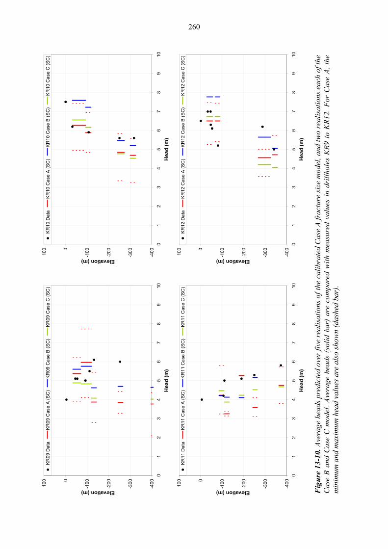
Multiple realisations of the three model cases A, B and C are considered, combining realisations of the background fractures for each model with stochastically generated hydrozone transmissivities (although hydrozone locations remain deterministically specified). For Case A, five realisations are performed, whereas for Cases B and C two realisations are calculated. Resultant baseline heads are aggregated, with mean values shown for each of the three model cases considered. In addition, for Case A, minimum and maximum heads across all simulations are presented.
Baseline heads for five realisations of the Case A site-scale models corresponding to 15 monitoring drillholes are shown in Figure 13-8 through Figure 13-11. Generally, measured baseline head and simulation results correlate above elevations of –300 m, with measured values realisable from the Hydro-DFN models; lying between the minimum and maximum values of predicted head for all simulations. The observed magnitude and sense of vertical gradients is reproduced by the model in most drillholes. For elevations around –300 m to –400 m, simulation results often under-predict measured head values in a number of drillholes. These discrepancies are likely caused by the effects of salinity which become significant around these elevations, and are neglected from the site-scale Hydro-DFN simulations (these are considered in the palaeohydrogeology simulations presented in Section 13.3, where the observed head measurements at depth are also reproduced). At shallow depths, a large range of baseline heads are predicted by the model, c. ±3m indicating a strong dependency on the model realisation considered. This is about the magnitude of variability with any given drillhole.
The averages over two realisations each of the site-scale Hydro-DFN model are shown in Figure 13-8 through Figure 13-11, for background fractures generated from the Case B and Case C fracture intensity-size models. These average head values with depth are comparable to the analysis of five realisation for Case A, again correlating well with measured values above -300m.
It is noted that although identical sections of the monitored drillholes were simulated for all model cases and realisations, for any given depth, head values may not always be available. This is caused when no fractures intersect with the sampled drillhole sections for a specific model case; a consequence of the sparse stochastic fracture networks generated.

258
-40
0
-30
0
-20
0
-10
00
100
01
23
45
67
89
10
Hea
d (
m)
Elevation (m)
KR
01 D
ata
KR
01
Cas
e A
(S
C)
KR
01 C
ase
B (
SC
)K
R01
Ca
se C
(S
C)
-40
0
-30
0
-20
0
-10
00
100
01
23
45
67
89
10
Hea
d (
m)
Elevation (m)
KR
02 D
ata
KR
02
Cas
e A
(S
C)
KR
02 C
ase
B (
SC
)K
R02
Ca
se C
(S
C)
-40
0
-30
0
-20
0
-10
00
100
01
23
45
67
89
10
Hea
d (
m)
Elevation (m)
KR
03 D
ata
KR
03
Cas
e A
(S
C)
KR
03 C
ase
B (
SC
)K
R03
Ca
se C
(S
C)
-40
0
-30
0
-20
0
-10
00
100
01
23
45
67
89
10
Hea
d (
m)
Elevation (m)
KR
04 D
ata
KR
04
Cas
e A
(S
C)
KR
04 C
ase
B (
SC
)K
R04
Ca
se C
(S
C)
Fig
ure
13-
8. A
vera
ge h
eads
pre
dict
ed o
ver
five
rea
lisa
tion
s of
the
cal
ibra
ted
Cas
e A
fra
ctur
e si
ze m
odel
, and
tw
o re
alis
atio
ns e
ach
of t
he
Cas
e B
and
Cas
e C
mod
el.
Ave
rage
hea
ds (
soli
d ba
r) a
re c
ompa
red
wit
h m
easu
red
valu
es i
n dr
illh
oles
KR
1 to
KR
4. F
or C
ase
A,
the
min
imum
and
max
imum
hea
d va
lues
are
als
o sh
own
(das
hed
bar)
.
258

259
-40
0
-30
0
-20
0
-10
00
100
01
23
45
67
89
10
Hea
d (
m)
Elevation (m)
KR
05 D
ata
KR
05
Cas
e A
(S
C)
KR
05 C
ase
B (
SC
)K
R05
Ca
se C
(S
C)
-40
0
-30
0
-20
0
-10
00
100
01
23
45
67
89
10
Hea
d (
m)
Elevation (m)
KR
06 D
ata
KR
06
Cas
e A
(S
C)
KR
06 C
ase
B (
SC
)K
R06
Ca
se C
(S
C)
-40
0
-30
0
-20
0
-10
00
100
01
23
45
67
89
10
Hea
d (
m)
Elevation (m)
KR
07 D
ata
KR
07
Cas
e A
(S
C)
KR
07 C
ase
B (
SC
)K
R07
Ca
se C
(S
C)
-40
0
-30
0
-20
0
-10
00
100
01
23
45
67
89
10
Hea
d (
m)
Elevation (m)
KR
08 D
ata
KR
08
Cas
e A
(S
C)
KR
08 C
ase
B (
SC
)K
R08
Ca
se C
(S
C)
Fig
ure
13-
9. A
vera
ge h
eads
pre
dict
ed o
ver
five
rea
lisa
tion
s of
the
cal
ibra
ted
Cas
e A
fra
ctur
e si
ze m
odel
, and
tw
o re
alis
atio
ns e
ach
of t
he
Cas
e B
and
Cas
e C
mod
el.
Ave
rage
hea
ds (
soli
d ba
r) a
re c
ompa
red
wit
h m
easu
red
valu
es i
n dr
illh
oles
KR
5 to
KR
8. F
or C
ase
A,
the
min
imum
and
max
imum
hea
d va
lues
are
als
o sh
own
(das
hed
bar)
.
259
260
-40
0
-30
0
-20
0
-10
00
100
01
23
45
67
89
10
Hea
d (
m)
Elevation (m)
KR
09 D
ata
KR
09
Cas
e A
(S
C)
KR
09 C
ase
B (
SC
)K
R09
Ca
se C
(S
C)
-40
0
-30
0
-20
0
-10
00
100
01
23
45
67
89
10
Hea
d (
m)
Elevation (m)
KR
10 D
ata
KR
10
Cas
e A
(S
C)
KR
10 C
ase
B (
SC
)K
R10
Ca
se C
(S
C)
-40
0
-30
0
-20
0
-10
00
100
01
23
45
67
89
10
Hea
d (
m)
Elevation (m)
KR
11 D
ata
KR
11
Cas
e A
(S
C)
KR
11 C
ase
B (
SC
)K
R11
Ca
se C
(S
C)
-40
0
-30
0
-20
0
-10
00
100
01
23
45
67
89
10
Hea
d (
m)
Elevation (m)
KR
12 D
ata
KR
12
Cas
e A
(S
C)
KR
12 C
ase
B (
SC
)K
R12
Ca
se C
(S
C)
Fig
ure
13-
10. A
vera
ge h
eads
pre
dict
ed o
ver
five
rea
lisa
tion
s of
the
cali
brat
ed C
ase
A fr
actu
re s
ize
mod
el, a
nd tw
o re
alis
atio
ns e
ach
of th
e C
ase
B a
nd C
ase
C m
odel
. A
vera
ge h
eads
(so
lid
bar)
are
com
pare
d w
ith
mea
sure
d va
lues
in
dril
lhol
es K
R9
to K
R12
. F
or C
ase
A,
the
min
imum
and
max
imum
hea
d va
lues
are
als
o sh
own
(das
hed
bar)
.
260

261
-400
-300
-200
-1000
100
01
23
45
67
89
10
Hea
d (
m)
Elevation (m)
KR
13 D
ata
KR
13
Ca
se A
(S
C)
KR
13 C
ase
B (
SC
)K
R1
3 C
ase
C (
SC
)
-400
-300
-200
-1000
100
01
23
45
67
89
10
Hea
d (
m)
Elevation (m)
KR
14 D
ata
KR
14
Ca
se A
(S
C)
KR
14 C
ase
B (
SC
)K
R1
4 C
ase
C (
SC
)
-400
-300
-200
-1000
100
01
23
45
67
89
10
Hea
d (
m)
Elevation (m)
KR
15 D
ata
KR
15
Ca
se A
(S
C)
KR
15 C
ase
B (
SC
)K
R1
5 C
ase
C (
SC
)
Fig
ure
13-
11. A
vera
ge h
eads
pre
dict
ed o
ver
five
rea
lisa
tion
s of
the
cali
brat
ed C
ase
A fr
actu
re s
ize
mod
el, a
nd tw
o re
alis
atio
ns e
ach
of th
e C
ase
B a
nd C
ase
C m
odel
. A
vera
ge h
eads
(so
lid
bar)
are
com
pare
d w
ith
mea
sure
d va
lues
in
drill
hole
s K
R13
to
KR
15.
For
Cas
e A
, th
e m
inim
um a
nd m
axim
um h
ead
valu
es a
re a
lso
show
n (d
ashe
d ba
r).
261

262
13.2 Pumping tests
Further confirmatory analysis of the Elaborated site-scale Hydro-DFN model involves calibration against pumping tests conducted at Olkiluoto site. Several pump and interference tests are recorded in /Vaittinen et al. 2008/ as performed between 1991 and 2004, of which four have been simulated and drawdowns predicted in both pumped and monitored drillhole sections. Details of the pumping tests considered are summarised in Table 13-2. Multiple realisations of the site-scale model are evaluated, with an abstraction rate applied to a specified drillhole, and subsequent drawdowns in both pumped and monitored drillholes associated with the interference tests compared with measured values. Multilevel piezometers are omitted from the models, with drawdowns only compared in KR drillholes.
Table 13-2. Summary of pumping tests simulated for confirmatory analysis.
Pumped drillhole
No. of monitored drillhole sections
Flow rate [L/min]
Drawdown in test section [m]
Test dates
KR4 16 17.0 17.8 17/02/98 – 03/03/98
KR1 10 * 36.4 17.0 02/04/92 – 15/04/92
KR7 11 15.4 10.0 18/04/95 – 22/04/95,
26/04/95 – 04/05/95
KR8 4 17.0 5.0 15/06/95 – 21/06/95
* excluding multilevel piezometer readings
13.2.1 Calibration of site-scale models
The changes to parameters required for calibration on the pumping tests was performed independently of those performed on the base line heads so as to identify the key parameters important to the two types of data independently. The consequences of both calibrations are considered in Section 13.2.3 and in the context of palaeohydrogeology in Section 13.6.
Confirmatory analyses are performed comparing predicted drawdown from steady-state Hydro-DFN simulations with measured values for the four pumping tests outlined in Table 13-2. Models are constructed identically to those for the baseline head analysis in Section 13.1, including a specified infiltration of 8mm/yr applied across the top surface boundary for elevations greater than zero (corresponding to Olkiluoto island), with zero head applied on the remainder of the top surface and at the lateral boundaries of the domain. To calculate the drawdown associated with a pumping test, two simulations are performed; one with and one without pumping at the drillhole. In each case, head values are calculated in the required drillhole test sections with drawdowns taken as the difference in groundwater head.
The four pumping tests simulated by the Hydro-DFN model are all of relatively short duration, c. 14 days or less. Steady-state calculations are performed, and compared with drawdown measurements at the end of pumping. Simple scoping calculations allow estimate of the time required for drawdowns to be observed at distances of 800m from the abstraction. Considering Hydrozones HZ20A and HZ20B, transmissivities at a
263
depth of –400 m are c. 2 10-6 m2/s, and analysis during excavation of ONKALO estimate storativity values of c. 2 10-5 /Vaittinen et al. 2010/. Thus pumping durations required for a response at 800m are approximately 19 days, longer than any of the pumping tests considered. Therefore, calibrations of site-scale models will focus on providing an acceptable match between simulated and measured drawdowns at the near monitoring drillholes. Accurate steady-state simulation of drawdowns measured at larger distances from the abstraction is not expected.
Calibrations of the transmissivities of stochastically generated background fractures are identical to the baseline head analysis with the changes detailed in Table 13-1 for Case A, B and C fracture intensity-size models. However, the calibration of hydrozone transmissivities is reconsidered to produce suitably transmissive connectivity between drillholes. Methods for generating hydrozone properties are detailed in Section 3.7 and consist of combining stochastically prescribed transmissivities for each hydrozone with deterministically specified local conditioning values inferred from PFL measurements at drillhole intersections. In section 13.1, changes were made to the transmissivities across the entirety of all hydrozones, with adjustments specified by depth. For the pumping test calibrations, transmissivities are adjusted in specific hydrozones only (see Table 13-3) as follows:
1. Local conditioning values at drillhole – hydrozone intersections are independently calibrated for all hydrozones starting from the original conditioning values for transmissivity detailed in /Vaittinen et al. 2011/, as inferred from PFL test inflows to drillholes. For pumping test simulations, the drawdowns observed in the monitoring drillholes are a consequence of the flowing connections, and thus transmissivity values are adjusted such that required flow rates are reproduced at the drillhole – hydrozone intersections to adequately represent the observed drawdowns.
2. For hydrozones HZ19A, HZ19B, HZ19C, HZ20A, and HZ20B only, the general changes to transmissivities suggested in Table 13-1 are made across the whole of each hydrozone along with the changes around drillhole intercepts detailed in Table 13-3.
Calibrations determine suitably transmissive connections between the pumped and monitored drillhole sections, such that the required drawdown is simulated. For the pumping tests considered, hydrozones HZ19A, HZ19B, HZ19C, HZ20A, and HZ20B dominate this local drillhole connectivity, and as such, the bulk transmissivity changes inferred from the baseline head analysis are only applied to these hydrozones (see point 2. above).
Calibrations are performed for several realisations of stochastic fractures, generated from Case A, B and C fracture intensity-size models with transmissivities semi-correlated to size. Corresponding heterogeneous hydrozones are also incorporated.
13.2.2 Calibrated predictions of drawdown
For five realisations of the Case A, and two realisations each of the Case B and C generated background fractures, local conditioning values for heterogeneous hydrozones are calibrated using four pumping tests. Sections of drillhole modelled are

264
based on packer locations described in /Vaittinen et al. 2008/, for which measured drawdowns were obtained. As for the preceding baseline head calibrations, to ensure sufficient likelihood that random fractures intersect with a given drillhole test section, packer locations are extended to a minimum length of 25 m where possible. In addition, for the pumping test in drillhole KR4, monitored sections in KR7(L5 through L2) are in close proximity, with KR7(L5 and L4) exhibiting identical drawdown, as do KR7(L3 and L2). Therefore, these two sets of monitored drillhole sections have been combined to yield representative section lengths of 25 m, and referred to from here on solely as KR7(L5) and KR7(L3), respectively. Adjustments to local conditioning transmissivities calibrated from the pumping test simulations, corresponding to point 1 above, as detailed in Table 13-3. It is noted that several of these changes are a consequence of the discretisation of the hydrozone into triangles of size 200 m on which local conditioning is applied, so where there are multiple drillhole intercepts within about 200 m on the same hydrozone, then one has to use the same conditioning value for each intercept, typically the largest transmissivity required to match the pumping test data.
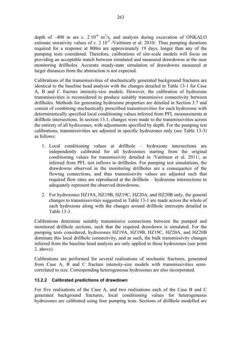
Simulation results for the four pumping tests outlined in Table 13-2 are shown in Figure 13-12 through Figure 13-15 respectively, detailing predicted drawdowns for each of the fracture size models Case A, Case B and Case C. Drawdowns for the calibrated model cases are compared with measured values, with monitoring drillholes ordered according to their Euclidian distance from the abstraction. Within the figures, intervals where the interpreted measured drawdown are considered to be uncertain by /Vaittinen et al. 2008/ are indicated by diagonal stripes.
Results for the pumping test in drillhole KR4 are shown in Figure 13-12, where the mean predicted drawdowns for all model cases correlate well with measurements in pumped drillhole KR4. Drawdown in monitored sections also correlate well with measurements, with the exception of KR1(L6 though L8), and KR5(L8 and L7), where all three model cases consistently over predict observed values. Over-prediction of drawdowns could be a consequence of compartmentalisation, i.e. insufficient connectivity between the monitored and pumped drillhole drillholes, or use of steady-state calculations with the limited time-scale of the pumping test; with head levels failing to stabilise in specific test sections, e.g. due to high storage. No results were available from either of the two realisations of the Case C model in monitored sections KR10(L4), KR7(L3) and KR9(L2).
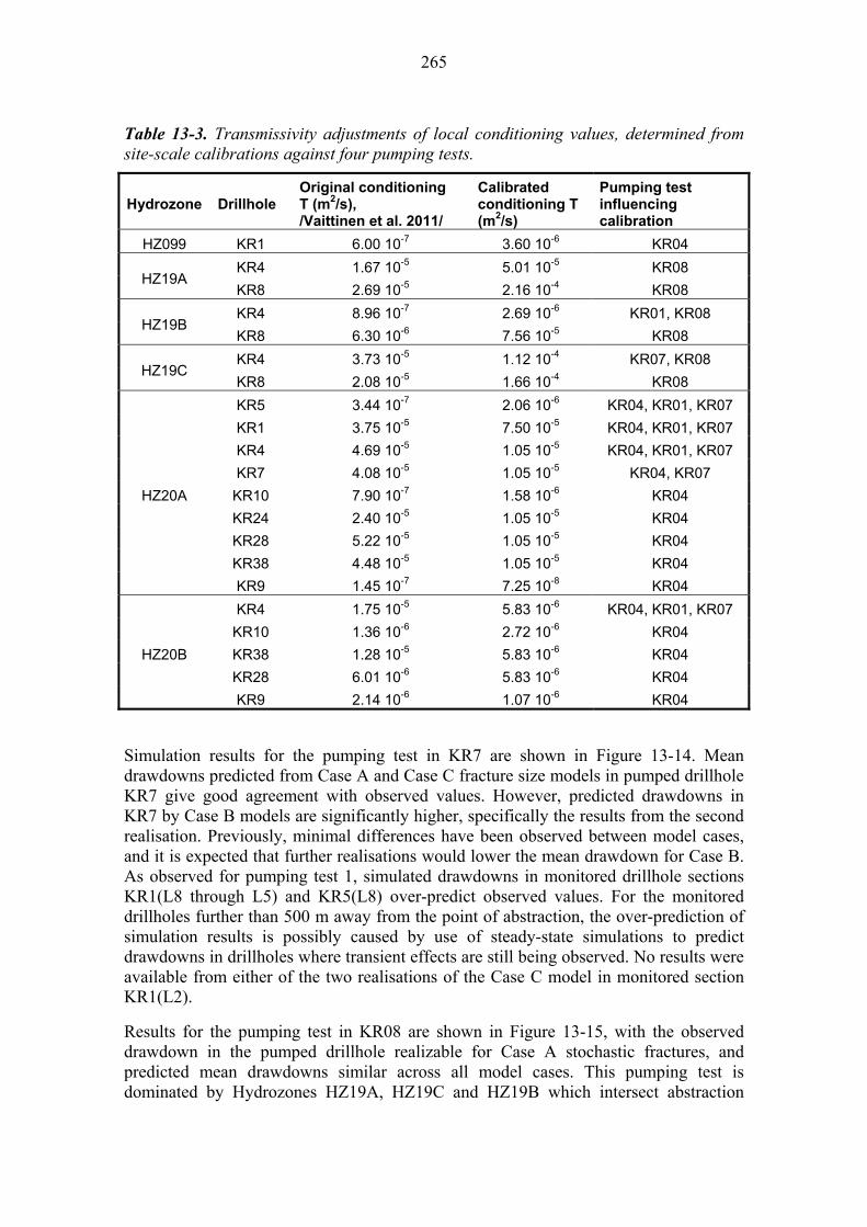
Comparison of measured drawdown with simulation results for the pumping of drillhole KR1 are shown in Figure 13-13. Although mean drawdowns in the pumped drillhole correlate well with observed values for all model cases, values in subsequent monitored sections generally over predict measurements. For Case A the five realisations suggest large variations in predicted drawdowns occur between realisations, with results sensitive to the model realisation considered. It is expected similar variation of results would be seen for Case B and Case C fracture size models if more realisations were considered. No results were available from either of the two realisations of the Case C model in monitored section KR5(L6). It was not possible to reduce the over-prediction of measured drawdowns in monitored drillholes further, as simulations proved insensitive to changes in the calibration values used. As such, the calibrations presented provide the best match possible to observed drawdowns using the current hydrozone description.
265
Table 13-3. Transmissivity adjustments of local conditioning values, determined from site-scale calibrations against four pumping tests.
Hydrozone Drillhole Original conditioning T (m2/s), /Vaittinen et al. 2011/
Calibrated conditioning T (m2/s)
Pumping test influencing calibration
HZ099 KR1 6.00 10-7 3.60 10-6 KR04
HZ19A KR4 1.67 10-5 5.01 10-5 KR08
KR8 2.69 10-5 2.16 10-4 KR08
HZ19B KR4 8.96 10-7 2.69 10-6 KR01, KR08
KR8 6.30 10-6 7.56 10-5 KR08
HZ19C KR4 3.73 10-5 1.12 10-4 KR07, KR08
KR8 2.08 10-5 1.66 10-4 KR08
HZ20A
KR5 3.44 10-7 2.06 10-6 KR04, KR01, KR07
KR1 3.75 10-5 7.50 10-5 KR04, KR01, KR07
KR4 4.69 10-5 1.05 10-5 KR04, KR01, KR07
KR7 4.08 10-5 1.05 10-5 KR04, KR07
KR10 7.90 10-7 1.58 10-6 KR04
KR24 2.40 10-5 1.05 10-5 KR04
KR28 5.22 10-5 1.05 10-5 KR04
KR38 4.48 10-5 1.05 10-5 KR04
KR9 1.45 10-7 7.25 10-8 KR04
HZ20B
KR4 1.75 10-5 5.83 10-6 KR04, KR01, KR07
KR10 1.36 10-6 2.72 10-6 KR04
KR38 1.28 10-5 5.83 10-6 KR04
KR28 6.01 10-6 5.83 10-6 KR04
KR9 2.14 10-6 1.07 10-6 KR04
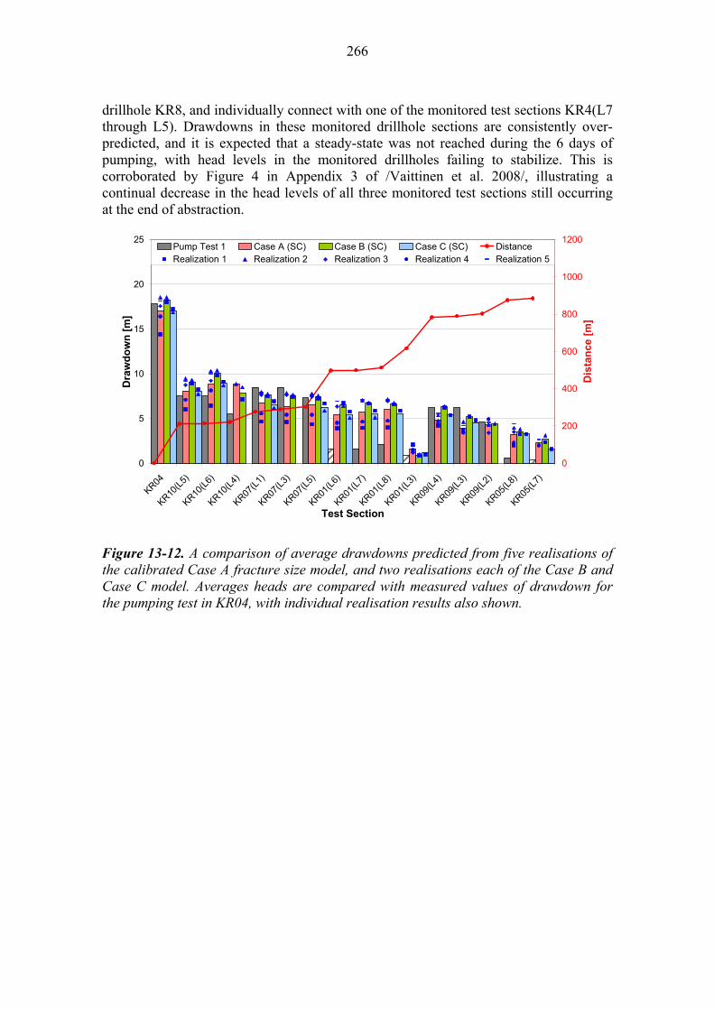
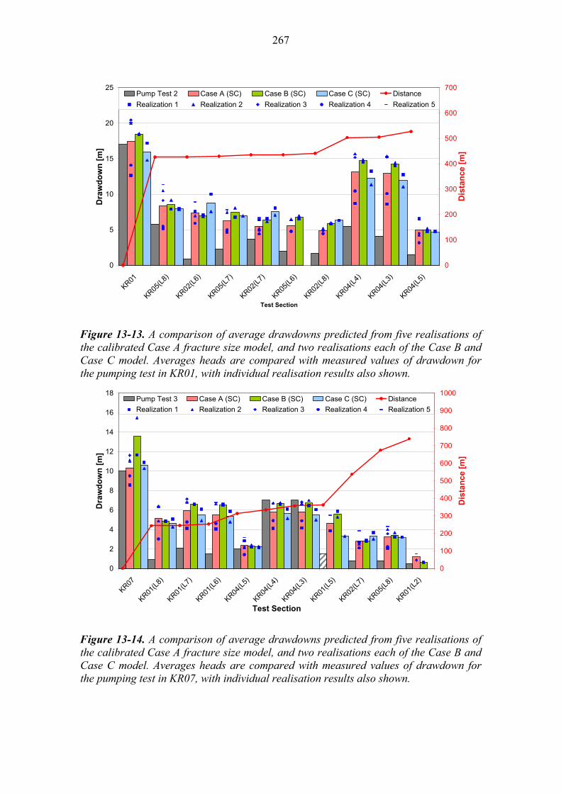
Simulation results for the pumping test in KR7 are shown in Figure 13-14. Mean drawdowns predicted from Case A and Case C fracture size models in pumped drillhole KR7 give good agreement with observed values. However, predicted drawdowns in KR7 by Case B models are significantly higher, specifically the results from the second realisation. Previously, minimal differences have been observed between model cases, and it is expected that further realisations would lower the mean drawdown for Case B. As observed for pumping test 1, simulated drawdowns in monitored drillhole sections KR1(L8 through L5) and KR5(L8) over-predict observed values. For the monitored drillholes further than 500 m away from the point of abstraction, the over-prediction of simulation results is possibly caused by use of steady-state simulations to predict drawdowns in drillholes where transient effects are still being observed. No results were available from either of the two realisations of the Case C model in monitored section KR1(L2).
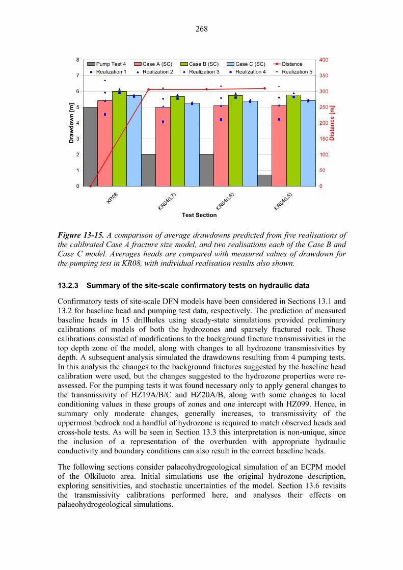
Results for the pumping test in KR08 are shown in Figure 13-15, with the observed drawdown in the pumped drillhole realizable for Case A stochastic fractures, and predicted mean drawdowns similar across all model cases. This pumping test is dominated by Hydrozones HZ19A, HZ19C and HZ19B which intersect abstraction
266
drillhole KR8, and individually connect with one of the monitored test sections KR4(L7 through L5). Drawdowns in these monitored drillhole sections are consistently over-predicted, and it is expected that a steady-state was not reached during the 6 days of pumping, with head levels in the monitored drillholes failing to stabilize. This is corroborated by Figure 4 in Appendix 3 of /Vaittinen et al. 2008/, illustrating a continual decrease in the head levels of all three monitored test sections still occurring at the end of abstraction.
0
5
10
15
20
25
KR04
KR10(L
5)
KR10(L
6)
KR10(L
4)
KR07(L
1)
KR07(L
3)
KR07(L
5)
KR01(L
6)
KR01(L
7)
KR01(L
8)
KR01(L
3)
KR09(L
4)
KR09(L
3)
KR09(L
2)
KR05(L
8)
KR05(L
7)
Test Section
Dra
wd
ow
n [
m]
0
200
400
600
800
1000
1200
Dis
tan
ce [
m]
Pump Test 1 Case A (SC) Case B (SC) Case C (SC) DistanceRealization 1 Realization 2 Realization 3 Realization 4 Realization 5
Figure 13-12. A comparison of average drawdowns predicted from five realisations of the calibrated Case A fracture size model, and two realisations each of the Case B and Case C model. Averages heads are compared with measured values of drawdown for the pumping test in KR04, with individual realisation results also shown.
267
0
5
10
15
20
25
KR01
KR05(L
8)
KR02(L
6)
KR05(L
7)
KR02(L
7)
KR05(L
6)
KR02(L
8)
KR04(L
4)
KR04(L
3)
KR04(L
5)
Test Section
Dra
wd
ow
n [
m]
0
100
200
300
400
500
600
700
Dis
tan
ce [
m]
Pump Test 2 Case A (SC) Case B (SC) Case C (SC) Distance
Realization 1 Realization 2 Realization 3 Realization 4 Realization 5
Figure 13-13. A comparison of average drawdowns predicted from five realisations of the calibrated Case A fracture size model, and two realisations each of the Case B and Case C model. Averages heads are compared with measured values of drawdown for the pumping test in KR01, with individual realisation results also shown.
0
2
4
6
8
10
12
14
16
18
KR07
KR01(L
8)
KR01(L
7)
KR01(L
6)
KR04(L
5)
KR04(L
4)
KR04(L
3)
KR01(L
5)
KR02(L
7)
KR05(L
8)
KR01(L
2)
Test Section
Dra
wd
ow
n [
m]
0
100
200
300
400
500
600
700
800
900
1000
Dis
tan
ce
[m]
Pump Test 3 Case A (SC) Case B (SC) Case C (SC) Distance
Realization 1 Realization 2 Realization 3 Realization 4 Realization 5
Figure 13-14. A comparison of average drawdowns predicted from five realisations of the calibrated Case A fracture size model, and two realisations each of the Case B and Case C model. Averages heads are compared with measured values of drawdown for the pumping test in KR07, with individual realisation results also shown.
268
0
1
2
3
4
5
6
7
8
KR08
KR04(L
7)
KR04(L
6)
KR04(L
5)
Test Section
Dra
wd
ow
n [
m]
0
50
100
150
200
250
300
350
400
Dis
tan
ce [
m]
Pump Test 4 Case A (SC) Case B (SC) Case C (SC) Distance
Realization 1 Realization 2 Realization 3 Realization 4 Realization 5
Figure 13-15. A comparison of average drawdowns predicted from five realisations of the calibrated Case A fracture size model, and two realisations each of the Case B and Case C model. Averages heads are compared with measured values of drawdown for the pumping test in KR08, with individual realisation results also shown.
13.2.3 Summary of the site-scale confirmatory tests on hydraulic data
Confirmatory tests of site-scale DFN models have been considered in Sections 13.1 and 13.2 for baseline head and pumping test data, respectively. The prediction of measured baseline heads in 15 drillholes using steady-state simulations provided preliminary calibrations of models of both the hydrozones and sparsely fractured rock. These calibrations consisted of modifications to the background fracture transmissivities in the top depth zone of the model, along with changes to all hydrozone transmissivities by depth. A subsequent analysis simulated the drawdowns resulting from 4 pumping tests. In this analysis the changes to the background fractures suggested by the baseline head calibration were used, but the changes suggested to the hydrozone properties were re-assessed. For the pumping tests it was found necessary only to apply general changes to the transmissivity of HZ19A/B/C and HZ20A/B, along with some changes to local conditioning values in these groups of zones and one intercept with HZ099. Hence, in summary only moderate changes, generally increases, to transmissivity of the uppermost bedrock and a handful of hydrozone is required to match observed heads and cross-hole tests. As will be seen in Section 13.3 this interpretation is non-unique, since the inclusion of a representation of the overburden with appropriate hydraulic conductivity and boundary conditions can also result in the correct baseline heads.
The following sections consider palaeohydrogeological simulation of an ECPM model of the Olkiluoto area. Initial simulations use the original hydrozone description, exploring sensitivities, and stochastic uncertainties of the model. Section 13.6 revisits the transmissivity calibrations performed here, and analyses their effects on palaeohydrogeological simulations.
269
13.3 Palaeohydrogeology calculations
13.3.1 Background
The evolution of the chemical composition of groundwaters in the Olkiluoto area is driven by the infiltration of waters with glacial, marine and meteoric origins, as determined by the climatological evolution (including the effects of glaciation, land-uplift and sea-level changes) of the site. The effects of this evolution on groundwater chemistry can therefore be thought of as a natural tracer experiment. The chemical composition of the groundwaters measured in the present day by analysis of groundwater samples from packed-off drillhole sections, can be compared to the predications of transient coupled groundwater flow and solute transport models. This comparison is intended as a verification of the Phase III site-scale models, in particular the upscaled properties of the Elaborated Hydro-DFN. Similar transport modelling has been carried out previously /Löfman et al. 2009/, based on the SDM 2008 /Posiva, 2009/.
Up to around 50,000 years ago the Weichselian glaciation covered most of Fennoscandian shield with ice sheets, depressing the bedrock elevation significantly /Eronen et al. (1995)/, /Eronen & Lehtinen (1996)/ and /Salonen et al. (2002)/. Complete Weichselian deglaciation started about 11,500 years ago, with Olkiluoto emerging from ice cover approximately 11,000 years ago. At this time Olkiluoto remained below the surface of the mildly saline Yoldia Sea. Glacial melt water associated with the retreating ice sheet was able to infiltrate the bedrock under pressure. The penetration depth is estimated at 200 m to 300m based on groundwater stable isotopic data /Pitkänen et al. 2004/.
The mildly saline Yoldia Sea stage was succeeded after a few hundred years by the fresh water Ancylus Lake stage (starting approximately 10,800 years ago) and the saline Littorina Sea stage (starting around 8500–8000 years ago). Because the Yoldia sea stage was relatively short, and the seawater of the Yoldia Sea was probably fairly dilute close to the ice margin because of the large volumes of glacial melt water, it is though that this stage did not significantly change the groundwater chemical composition. The peak salinity of the Littorina Sea has been estimated to be about 12 g/L /Westman et al. 1999/. Since then the salinity of the seawater has been reduced steadily to its current value of about 6 g/L.
As a result of land rebound and sea level changes, Olkiluoto island begun to emerge from the Baltic Sea about 3000–2500 years ago /Eronen & Lehtinen 1996/. The infiltration of fresh meteoric water from precipitation dates from this stage in the evolution of the site.
The following five reference waters have been defined in order to model the palaeohydrogeological evolution of the groundwater, for the different geological stages at Olkiluoto over the last 10,000 years:
Brine: This is ancient water found at depth, characterised by high salinity and high chloride content (> 20,000 mg/L). Its non-marine origin is evident in its low magnesium content (< 20 mg/L). It has enriched δ18O levels.

270
Littorina: Representing Littorina and Baltic Sea water. It is characterised by high S04 content (~ 300 mg/L). Its saline source implies moderate chloride content (max. ~ 5,500 mg/L) (for comparison Baltic Sea water has a present-day chloride content of ~ 3,000 mg/L). Its marine origin also implies high magnesium content (max. 250-350 mg/L). It has enriched δ18O (> -10 ‰ VSMOW).
Meteoric: Representing water due to precipitation infiltrating though the ground surface. Since the models are chemically conservative, the composition of this reference water also accounts for near surface interactions of the infiltrating water with the near surface bedrock and quaternary deposits. It is characterised by high HCO3 content (~ 450 mg/L). Its non-saline source implies low chloride content (< 200 mg/L). A non-marine origin implies low magnesium content (< 50 mg/L). It has intermediate δ18O (-12 to -11 ‰ VSMOW) levels.
Glacial: Representing glacial melt water, it is characterised by significantly depleted δ18O levels. A non-saline source implies low chloride content (< 8 mg/L). A non-marine origin implies low magnesium content (< 8 mg/L).
Subglacial: Representing ancient water, it is composed of meteoric and brackish waters from periods before the Weichselian glaciation. Strong saline source implies high chloride content (> 20,000 mg/L). Its non-marine origin implies low magnesium content (< 50 mg/L). It has intermediate δ18O concentrations (-12 to -11 ‰ VSMOW).
The chemical composition of each reference water is listed in Table 13-4, taken from /Pitkänen 2010/, based on /Partamies and Pitkänen 2012/.
Table 13-4. Chemical composition assumed for each of the reference waters.
Chemical Reference water
Brine Littorina Meteoric Glacial Subglacial
TDS (g/L) 68.8 11.9 0.5 0.0 4.9
Cl (g/L) 43.000 6.500 0.060 0.001 3.000
HCO3 (g/L) 0.012 0.093 0.291 0.000 0.013
SO4 (g/L) 0.001 0.890 0.048 0.001 0.001
Mg (g/L) 0.002 0.448 0.016 0.000 0.027
Br (g/L) 0.348 0.022 0.000 0.000 0.021
δ2H (0/00-VSMOW)
-49.8 -37.8 -82.1 -166.0 -86.0
δ18O (0/00 -VSMOW)
-10.1 -4.7 -11.5 -22.0 -12.0
Na (g/L) 9.750 3.674 0.025 0.000 1.350
K (g/L) 0.022 0.134 0.007 0.000 0.005
Ca (g/L) 15.700 0.151 0.092 0.000 0.510

271
Groundwater chemistry can affect groundwater movement by changing the density or the viscosity of the groundwater. These density changes are likely to be dominated by the presence of dissolved salt. Since gradients in the water table at Olkiluoto are expected to be relatively weak because of the gentle topography, the buoyancy forces arising from density variations in the groundwater are relatively significant.
The conceptual model of the evolution of the groundwaters can be expressed in terms of the reference waters as follows: It is thought that below around -400 m elevation Brine water and Subglacial water have remained undisturbed for long time periods, due to the predicted low flow rates at this depth. Above this elevation groundwater mixing can take place driven through a combination of buoyancy forces arising from differences in groundwater density and pressure differences arising from changes in the ground surface elevation.
Immediately after the Weichselian deglaciation it is thought that the glacial melt water associated with the retreating ice sheet was able to infiltrate the bedrock under pressure. Hence an initial condition for subsequent modelling specifies that above the Brine water, the groundwater is composed of Glacial and Subglacial waters.
During the Littorina Sea and Baltic Sea stages the denser sea waters are expected to displace the less dense Glacial and Subglacial waters. Since Olkiluoto is under-water at this stage this flow is purely density driven. The infiltration to depth stops only when the Littorina and Baltic Sea waters encounter the more dense Brine water. The variation in salinity of the Littorina and Baltic Seas over time can be conceptualised as a variable mixture of the Littorina and Meteoric reference waters for modelling purposes.
When Olkiluoto island emerges from the Baltic Sea around 3,000 years ago Meteoric water starts to infiltrate and mix with the pre-existing groundwaters. Meteoric water is less dense than the predominately Littorina water that it encounters, therefore in order to displace this water the driving heads must be sufficient to overcome the opposing buoyancy forces.
The process of rock-matrix diffusion is thought to be important in understanding the chemical evolution of the groundwater at Olkiluoto /Löfman et al. 2009/. In fractured rocks, most of the groundwater flow takes place through a network of interconnected fractures, which comprise the kinematic porosity. In addition to the kinematic porosity, the rock matrix is itself porous. Solutes can be transported by diffusion from the pore water in the kinematic porosity into the relatively immobile water in the low permeability rock matrix. This is a retardation mechanism, because solutes would otherwise be transported at a velocity determined by the groundwater flux and the accessible kinematic porosity. Rock matrix diffusion also acts as mixing process, since solutes that have diffused into the rock matrix can diffuse back out over a period of time, acting as an immobile reservoir for solutes. 13.3.2 Data analysis
Before describing the modelling work in Section 13.3.3 we review the data available for comparison, and present some interpretations in terms of the conceptual model of reference water transport and mixing. The data is of two types: head data and chemistry data. The analysis of the data is in terms of the influence due to:

272
Elevation;
Surface topography;
Thickness of the overburden;
Proximity to hydrozones.
Head data
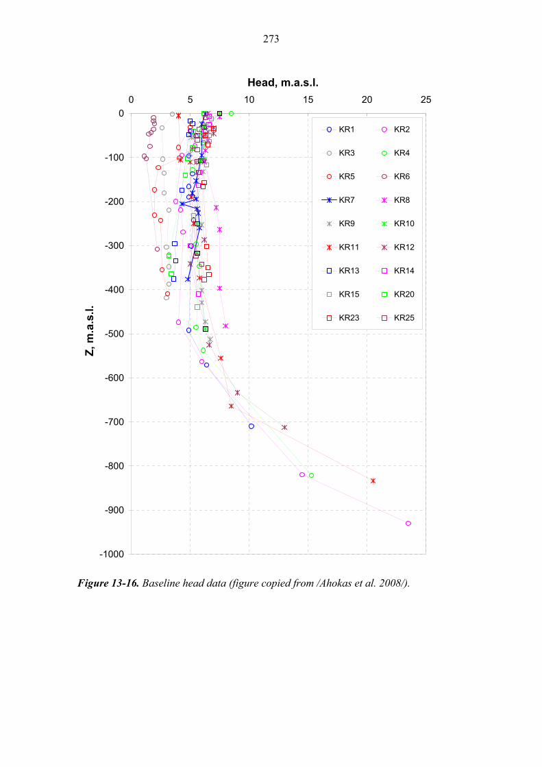
The distribution of head with elevation from 19 drillholes is plotted in a summary figure of all the determined baseline heads, shown in Figure 13-16. The locations of the drillholes are shown in Figure 2-2. At the surface the heads vary between 2 m to 9 m. In several drillholes a decreasing trend with depth can be observed to an elevation of approximately –50 m. Below an elevation of –100 m a weak increasing trend is apparent, whilst a strong increasing trend is seen below an elevation of –500 m due to the increasing salinity of the groundwater.
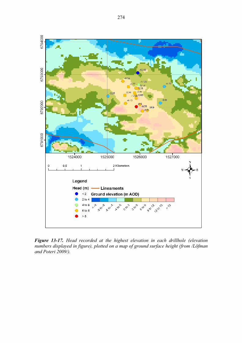
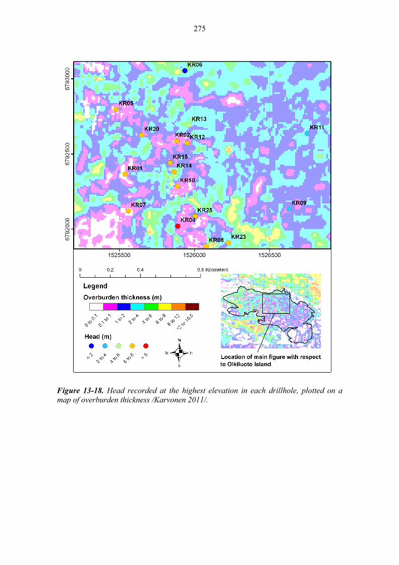
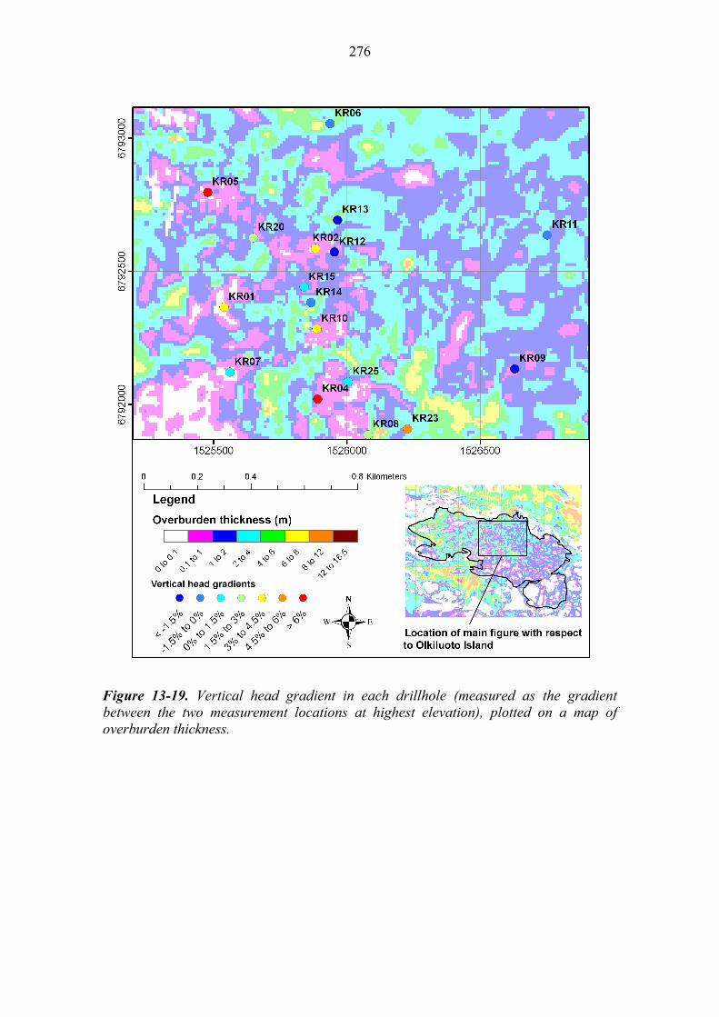
Figure 13-17 shows that the heads recorded at the top of each drillhole correlates closely with the ground elevation at that location. The lowest heads were determined for drillhole KR6, which is close to the sea (Figure 13-18 shows the positions of drillholes). The highest values were from KR4 and are likely to be caused by the effect of local elevated regions. Figure 13-18 and Figure 13-19 do not suggest a clear correlation between overburden thickness and either the heads at the top of the drillholes, or the vertical head gradients at the top of the drillholes.
Figure 13-20 suggests notable steps in head seen in drillholes KR5, KR9 and KR11 could be caused by hydraulic connections along hydrozones to the sea. In particular HZ19C is interpreted to intersect KR9 and KR11 at the approximate elevation of the observed head drops. Similarly, HZ20A is predicted to intersect KR5 at the approximate elevation of the observed head drop. There are also many instances of hydrozones intersecting drillholes without any observed effect on the heads, suggesting heterogeneity in the hydraulic properties both within hydrozones and between different hydrozones.
273
-1000
-900
-800
-700
-600
-500
-400
-300
-200
-100
0
0 5 10 15 20 25
Head, m.a.s.l.Z
, m.a
.s.l
.
KR1 KR2
KR3 KR4
KR5 KR6
KR7 KR8
KR9 KR10
KR11 KR12
KR13 KR14
KR15 KR20
KR23 KR25
Figure 13-16. Baseline head data (figure copied from /Ahokas et al. 2008/).
274
Figure 13-17. Head recorded at the highest elevation in each drillhole (elevation numbers displayed in figure), plotted on a map of ground surface height (from /Löfman and Poteri 2009/).
275
Figure 13-18. Head recorded at the highest elevation in each drillhole, plotted on a map of overburden thickness /Karvonen 2011/.
276
Figure 13-19. Vertical head gradient in each drillhole (measured as the gradient between the two measurement locations at highest elevation), plotted on a map of overburden thickness.

277
Figure 13-20. Head measured in each drillhole section, with selected hydrozones.
Hydrochemical data
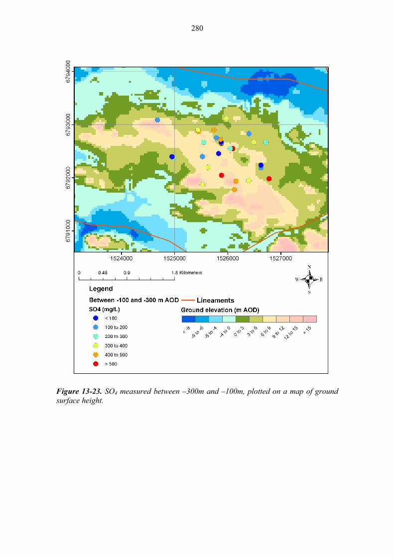
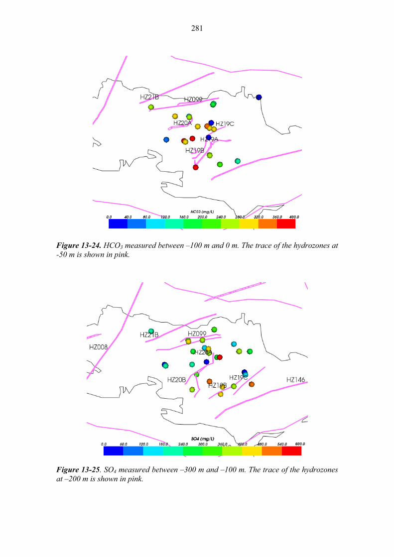
The chemistry data presented in Section 3.4 suggest the following interpretations, in terms of the defined reference waters.
Meteoric water, characterised by high HCO3 concentrations, has infiltrated the bedrock to an elevation of –100 m to –150 m;
Littorina water, characterised by high SO4 concentrations, remains at significant mass fractions at elevations between –100 m and –300 m;
Saline water, characterised by high Cl concentrations, is present with increasing concentration fraction below approximately –400 m. There is a slight step in the Cl concentration at elevations between –100 m and –300 m which could be due to the contribution of Littorina water.
The Cl concentrations can be matched approximately if we assume the following relationship for the mass fraction of Saline water with depth:
Mass fraction of Saline =
200
)800(zExp (13-1)
where z is elevation, and the expression is bounded by 0 and 1. The match to the data is shown in Figure 13-21. This has a very similar functional form to that used in /Löfman et al. 2009/.

278
Cl concentrations versus elevation
-900
-800
-700
-600
-500
-400
-300
-200
-100
0
100
0 10,000 20,000 30,000 40,000 50,000 60,000
Cl (mg/L)
Ele
vati
on
(m
)Fit to data
Data
Figure 13-21. Measured Cl concentration in fracture water versus elevation along with the fit suggested in Equation (13-1).
Simple scoping calculations can be made for the infiltration distances of Littorina and Meteoric waters, based on some simple assumptions. Based on Table 13-4 the fluid densities of the reference waters can be approximated as 1000 kg/m3 for Glacial water, a density for Meteoric water of 1001 kg/m3, a density of 1008 kg/m3 for Littorina water and a density of 1068 kg/m3 for Brine water. Assuming that Littorina water is displacing a mixture of Brine water and Glacial water, based on Equation (13-1), then we find that the mixture has the same salinity as Littorina water at –360 m. Since this is approximately the depth of infiltration measured, this scoping calculation suggests that the Littorina water had time to infiltrate the fracture pore space and sink under gravity until it balanced the buoyancy of the pre-existing Brine/Glacial mix. Although it may not have had time to equilibrate with the rock matrix prior to Olkiluoto starting to rise from the sea 3000 to 2500 years ago.
In each of the graphs presented in Section 3.4 there is considerable variability in the measured concentrations with elevation. This variability could be caused by many factors; here the data is analysed in terms of topographic surface elevation and proximity to mapped hydrozones, representing two possible influences.
Figure 13-22 suggests that HCO3 measurements above –100 m are influenced by surface topography, with higher concentrations measured in areas of higher elevation. This is likely to arise because higher elevations are associated with recharge areas

279
where recent Meteoric waters are infiltrating. Also, areas of higher elevation have been exposed to precipitation for longer time periods, giving more time for Meteoric water to infiltrate.
Figure 13-23 shows a map of surface topography with SO4 measurements at elevations between –100 m and –300 m. There is no obvious correlation between surface topography and SO4 concentration, suggesting that the influence of surface topography is not significant below approximately –100 m.
Figure 13-24 shows HCO3 concentrations above –100 m relative to the upper parts of hydrozones. There are high and low values close to hydrozones and in the rock mass between hydrozones. Figure 13-25 suggests a possible influence of hydrozones HZ19, HZ20 and HZ099 on SO4 concentrations between -100 m and –300 m, but again the spatial correlation is not conclusive. Overall then there is not a conclusive difference between hydrogeochemistry in hydrozones compared to the rock mass.
Figure 13-22. HCO3 measured above –100 m, plotted on a map of ground surface height.
280
Figure 13-23. SO4 measured between –300m and –100m, plotted on a map of ground surface height.
281
Figure 13-24. HCO3 measured between –100 m and 0 m. The trace of the hydrozones at -50 m is shown in pink.
Figure 13-25. SO4 measured between –300 m and –100 m. The trace of the hydrozones at –200 m is shown in pink.
282
13.3.3 Model definition
Solute transport and rock matrix diffusion
Salinity arises from a number of groundwater constituents. This is modelled in terms of the transport of fractions of selected reference waters. A reference water is defined in terms of concentrations of its chemical constituents such as chloride, sodium, etc. Each reference water is chosen to represent groundwater from a particular origin or location. For example, reference waters have been defined to represent both ancient Brines and more recent Meteoric waters arising from precipitation.
An ECPM model has been used to represent coupled groundwater flow and solute transport. The flow of groundwater of variable-density, allowing for rock-matrix diffusion, has been modelled using the following equations /Hoch and Jackson 2004/:
)( gk
q
P , (13-2)
0)()(
q
tf , (13-3)
0
)()()(
wif
f
w
cDcc
t
c
Dq , (13-4)
)()(
w
cD
wt
ci
, (13-5)
where (bold characters indicate vector or tensor quantities)
q is the specific discharge (or Darcy flux) [LT-1];
k is the effective permeability tensor due to the fractures carrying the flow [L2]; is the groundwater viscosity (which depends on the salinity) [ML-1T-1]; P is the (total) pressure in the groundwater [ML-1T-2]; is the groundwater density (which depends on the salinity) [ML-3]; g is the gravitational acceleration [LT-2]; t is the time [T];
f is the effective porosity due to the fractures carrying the flow (which is
sometimes referred to as the kinematic porosity) [-]; c is the salinity in the groundwater flowing through the fractures (expressed as a mass fraction) [-]; D is the (effective) dispersion tensor [L2T-1];
v
vD jiTLijTijmD
,
and,
283
mD is the molecular diffusivity;
L is the longitudinal dispersion length for a given rock type;
T is the transverse dispersion length for a given rock type; v is the pore water velocity vector ( /qv ).
iD is the intrinsic diffusion coefficient into the rock matrix [L2T-1];
is the specific fracture surface area, which is the average surface area of the matrix per unit volume [L-1]. It is based on the volume of rock. (For smooth planar fractures, is given by 2P32, where P32 is the fracture area per unit volume, which is a measure of fracture intensity);
w is a coordinate in the rock matrix [L]; c is the solute concentration of the groundwater in the rock matrix
(expressed as a mass fraction) [-]; is the capacity factor of the rock matrix [-]. For a non-sorbing solute this is taken to be equal to the Diffusion accessible porosity, m [-].
The equations above are equivalent to Darcy’s law, conservation of groundwater mass, conservation of groundwater solute in the fractures (allowing for diffusion into the rock matrix) and an equation for diffusion into the rock matrix. In modelling the migration of salinity, the capacity factor has been taken to be equal to the diffusion accessible porosity in the rock matrix, m .
The equations given above have to be supplemented by appropriate boundary and initial conditions. Suitable boundary conditions for the groundwater flow equations are prescriptions of either the groundwater pressure or the groundwater flux around the boundary of the domain modelled. Suitable boundary conditions for the equation for the transport of solutes are prescriptions of the solutes in the fractures at the domain boundary or the flux of solutes into the groundwater in the fractures. The boundary conditions for the diffusion equation are that the solutes in the groundwater in the matrix at the fracture surface is equal to the solute in the groundwater in the fractures locally:
cwc )0( ; (13-6)
and that the flux of solute in the matrix is zero at the maximum penetration depth d into the matrix:
0)(
dww
cDi . (13-7)
If the model is used to represent diffusion into the entire rock matrix between the fractures, d would be taken to be equal to half the fracture spacing (because solutes could diffuse into the block from the fractures on either side of the block). The model could also be used to represent cases in which the distance that solute can diffuse into the rock matrix is more limited.
284
In the modelling, groundwater density and viscosity vary spatially in three dimensions based on equations of state that are a function of total groundwater salinity, total pressure, and temperature. The salinity for a given water composition is simply the sum over reference waters of the product of the reference water fraction and the salinity of that reference water. The salinities for the reference waters were calculated from the Total Dissolved Solids (TDS, g L-1) using:
Salinity = TDS / ρ, (13-8)
where density is a function of salinity (and temperature, and total pressure). The density and viscosity were obtained using empirical correlations for NaCl brines /Laaksoharju et al. 2005/ and /Kestin et al. 1981/.
Model domain and grid
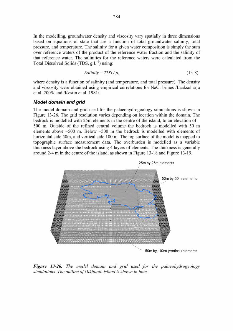
The model domain and grid used for the palaeohydrogeology simulations is shown in Figure 13-26. The grid resolution varies depending on location within the domain. The bedrock is modelled with 25m elements in the centre of the island, to an elevation of –500 m. Outside of the refined central volume the bedrock is modelled with 50 m elements above –500 m. Below –500 m the bedrock is modelled with elements of horizontal side 50m, and vertical side 100 m. The top surface of the model is mapped to topographic surface measurement data. The overburden is modelled as a variable thickness layer above the bedrock using 4 layers of elements. The thickness is generally around 2-4 m in the centre of the island, as shown in Figure 13-18 and Figure 13-19.
Figure 13-26. The model domain and grid used for the palaeohydrogeology simulations. The outline of Olkiluoto island is shown in blue.

285
Boundary conditions
Boundary conditions are used in the palaeohydrogeology simulations of Olkiluoto to:
Describe the flow of groundwater through the bottom and sides of the modelled domain;
Implement the recharge due to precipitation when the surface of Olkiluoto Island is above sea level;
Implement a specified pressure boundary condition on the sea bed;
Model the interface between the less refined outer region of the model domain and the more refined inner region of the model domain;
Describe the evolution of the groundwater composition on the top surface of the model;
Describe the transport of reference waters at the bottom and sides of the modelled domain.
No-flow boundary conditions are imposed on the bottom and sides of the model.
The modelling of heads and pumping tests in Sections 13.1 and 13.2 ignored groundwater in the overburden and set a specified infiltration of 8mm/year on the top of the bedrock. Here, a representation of the overburden is included and the recharge to the saturated zone within it is considered. In order to implement the recharge due to precipitation, the recharge flux, R, into or out of the model is defined as a function of the current head, h, in the model, the topographic surface elevation, z, and the maximum potential groundwater recharge, Rp. The potential groundwater recharge to the saturated zone is equal to the precipitation minus evapo-transpiration (P-E) and minus overland flow and flow through the unsaturated zone (Rp=P-E-Qs). Overland flow and flow through the unsaturated zone are subtracted since only the potential recharge to the saturated zone is of interest. Appropriate functions for the flux, R, must have certain characteristics. For recharge areas, the head, h, or water table, is below ground surface and so the recharge must be equal to the full recharge, Rp. In discharge areas, the water table is just above ground surface and so head is just above ground surface, which can be achieved by taking a suitably large flux out of the model, i.e. a negative value of R, whenever the head goes above ground surface. The function used is:
00
0
/)(
1exp
zzzhR
zzzh
RR
p
p
, (13-9)
where ε and δ are small numbers (0.15 and 0.005, respectively), and z0 is the elevation of the shoreline. This function implies that if the water table is more than ε below the topographic surface then recharge equals the full potential groundwater recharge. Above that, the recharge reduces until the water table is at the surface. If the water table is above the topographic surface, then recharge becomes negative, i.e. discharge, and an appropriate flux of groundwater is taken from the model to reduce the head until the
286
water table is restored to just above topographic height. Hence, this boundary condition is a non-linear equation (the flux depends on the free-variable head) that ensures a specified flux if the water table is low and a specified head where the water table is at or above ground surface. Newton-Raphson iteration was used to achieve convergence of the non-linear equations at each time-step. This technique works best for systems with smooth gradients as used here.
It should be noted that in this model any groundwater that discharges through the top surface exits the model and does not enter a separate surface model that allows recharge downstream.
When simulating the palaeohydrogeology over the last 8,000 years, transient variations in surface boundary conditions have to be considered both due to changes in the shoreline and the salinity of the Littorina/Baltic sea. The evolution of surface and hydrology and methods of coupling these to models of groundwater flow in the bedrock has been studied in detail in /Karvonen 2011/. The approach used here is to apply the same definition of the boundary conditions as detailed above, but to calculate heads and elevations relative to a sea-level datum that evolves in time. ConnectFlow uses residual pressure, PR, as the independent flow variable which is related to total pressure, PT, by
)( 00 zzgPP TR , (13-10)
where ρ0 is the density of freshwater, g is acceleration due to gravity, and z is the elevation of the point. For transients, the datum, z0=z0(t), varies in time according to the shoreline curve defined by /Löfman et al. 2009/ (Chapter 3 therein), z0(t), see Figure 13-27 and Figure 13-29.
For the area under the sea, it is most natural to use a specified head type boundary condition, where the head is equal to the depth of the sea multiplied by ρs/ρ0, where ρs is density of the Baltic Sea and ρ0 is fresh water density.
The composition of the groundwater infiltrating the top surface of the model offshore was taken to be a mixture of Littorina and Meteoric reference waters, with the proportion of each determined by the prescribed salinity of the sea, as shown in Figure 13-28. Onshore the infiltrating reference water was assumed to be Meteoric.
The solute boundary condition on the vertical sides of the model was taken to be zero solute flux. The solute boundary condition on the bottom of the model was taken to be fixed and equal to the initial condition, as described below.
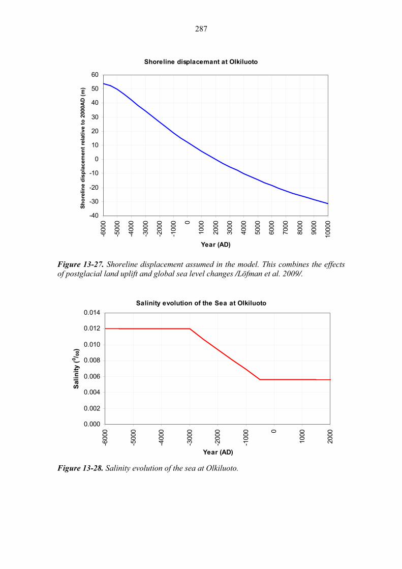
287
Shoreline displacemant at Olkiluoto
-40
-30
-20
-10
0
10
20
30
40
50
60
-600
0
-500
0
-400
0
-300
0
-200
0
-100
0 0
1000
2000
3000
4000
5000
6000
7000
8000
9000
1000
0
Year (AD)
Sh
ore
line
dis
pla
cem
ent
rela
tive
to
200
0AD
(m
)
Figure 13-27. Shoreline displacement assumed in the model. This combines the effects of postglacial land uplift and global sea level changes /Löfman et al. 2009/.
Salinity evolution of the Sea at Olkiluoto
0.000
0.002
0.004
0.006
0.008
0.010
0.012
0.014
-600
0
-500
0
-400
0
-300
0
-200
0
-100
0 0
1000
2000
Year (AD)
Sal
init
y (0 / 0
0)
Figure 13-28. Salinity evolution of the sea at Olkiluoto.
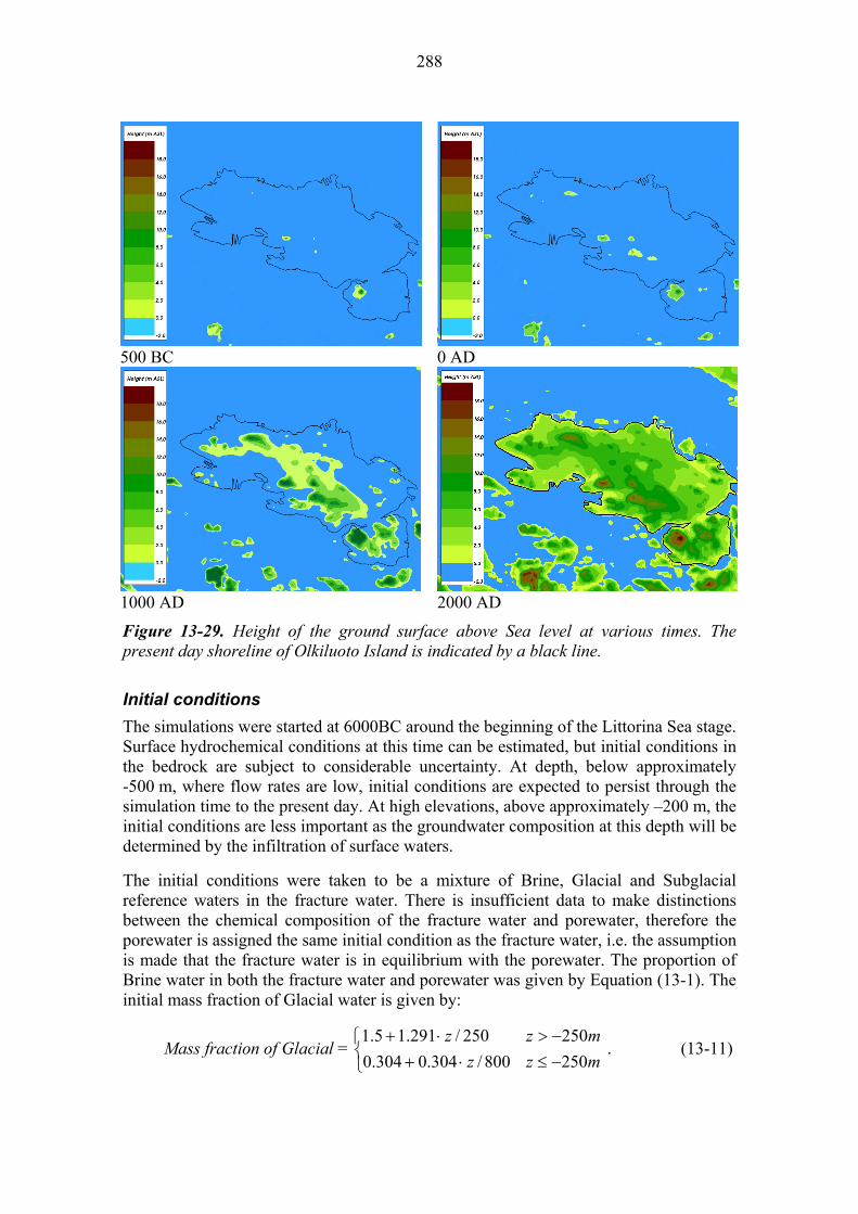
288
500 BC 0 AD
1000 AD 2000 AD
Figure 13-29. Height of the ground surface above Sea level at various times. The present day shoreline of Olkiluoto Island is indicated by a black line.
Initial conditions
The simulations were started at 6000BC around the beginning of the Littorina Sea stage. Surface hydrochemical conditions at this time can be estimated, but initial conditions in the bedrock are subject to considerable uncertainty. At depth, below approximately -500 m, where flow rates are low, initial conditions are expected to persist through the simulation time to the present day. At high elevations, above approximately –200 m, the initial conditions are less important as the groundwater composition at this depth will be determined by the infiltration of surface waters.
The initial conditions were taken to be a mixture of Brine, Glacial and Subglacial reference waters in the fracture water. There is insufficient data to make distinctions between the chemical composition of the fracture water and porewater, therefore the porewater is assigned the same initial condition as the fracture water, i.e. the assumption is made that the fracture water is in equilibrium with the porewater. The proportion of Brine water in both the fracture water and porewater was given by Equation (13-1). The initial mass fraction of Glacial water is given by:
Mass fraction of Glacial =
mzz
mzz
250800/304.0304.0
250250/291.15.1 . (13-11)

289
This equation is subject to the additional constraints that the mass fractions of Glacial water is less than or equal to one and greater than or equal to zero. Subglacial water makes up the remainder of the prescription. The mass fraction of Glacial water for the initial condition was estimated based on the δ2H and δ18O measurements at depth (see Figure 13-30 and Figure 13-31), and these should not change significantly over the duration of the simulations due to the low flow-rates below about –300 m. The initial condition is illustrated in Figure 13-32.
H2 concentration versus elevation
-900
-800
-700
-600
-500
-400
-300
-200
-100
0
100
-150 -125 -100 -75 -50
H2 (0/00 VSMOW)
Ele
vati
on
(m
)
Data
Initial conditionl
Figure 13-30. The initial δ2H composition compared to the measured data.
d18O concentrations versus elevation
-900
-800
-700
-600
-500
-400
-300
-200
-100
0
100
-20 -15 -10 -5 0
d18O (0/00 VSMOW)
Ele
vati
on
(m
)
Data
Initial condition
Figure 13-31. The δ18O composition compared to the measured data.
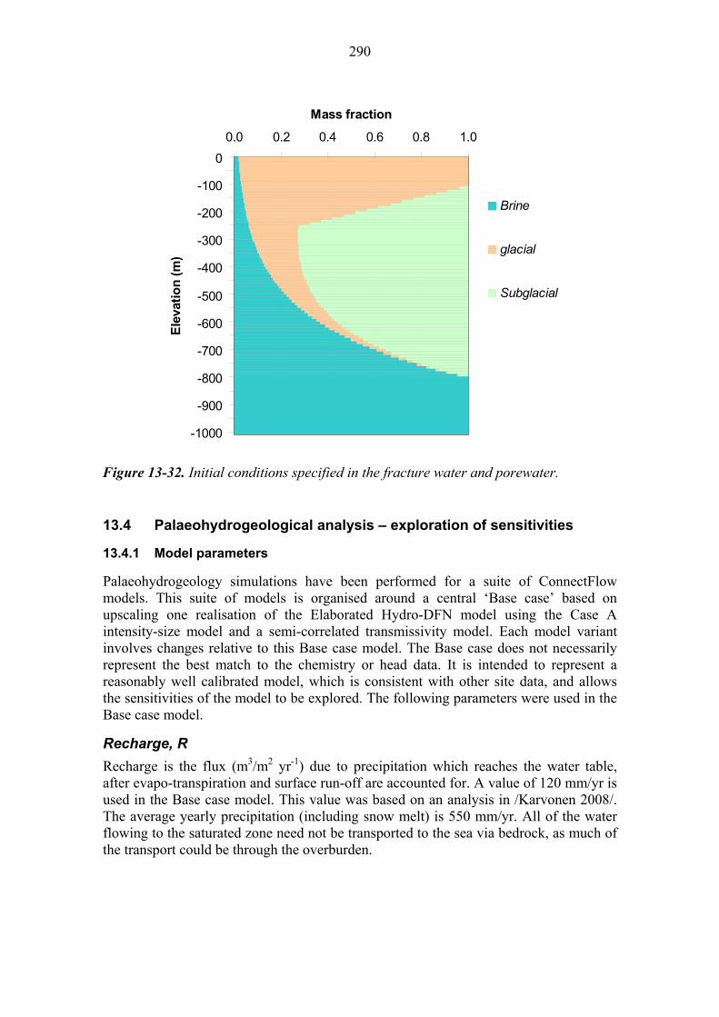
290
0.0 0.2 0.4 0.6 0.8 1.0
0
-100
-200
-300
-400
-500
-600
-700
-800
-900
-1000
Ele
vati
on
(m
)
Mass fraction
Brine
glacial
Subglacial
Figure 13-32. Initial conditions specified in the fracture water and porewater.
13.4 Palaeohydrogeological analysis – exploration of sensitivities
13.4.1 Model parameters
Palaeohydrogeology simulations have been performed for a suite of ConnectFlow models. This suite of models is organised around a central ‘Base case’ based on upscaling one realisation of the Elaborated Hydro-DFN model using the Case A intensity-size model and a semi-correlated transmissivity model. Each model variant involves changes relative to this Base case model. The Base case does not necessarily represent the best match to the chemistry or head data. It is intended to represent a reasonably well calibrated model, which is consistent with other site data, and allows the sensitivities of the model to be explored. The following parameters were used in the Base case model.
Recharge, R
Recharge is the flux (m3/m2 yr-1) due to precipitation which reaches the water table, after evapo-transpiration and surface run-off are accounted for. A value of 120 mm/yr is used in the Base case model. This value was based on an analysis in /Karvonen 2008/. The average yearly precipitation (including snow melt) is 550 mm/yr. All of the water flowing to the saturated zone need not be transported to the sea via bedrock, as much of the transport could be through the overburden.
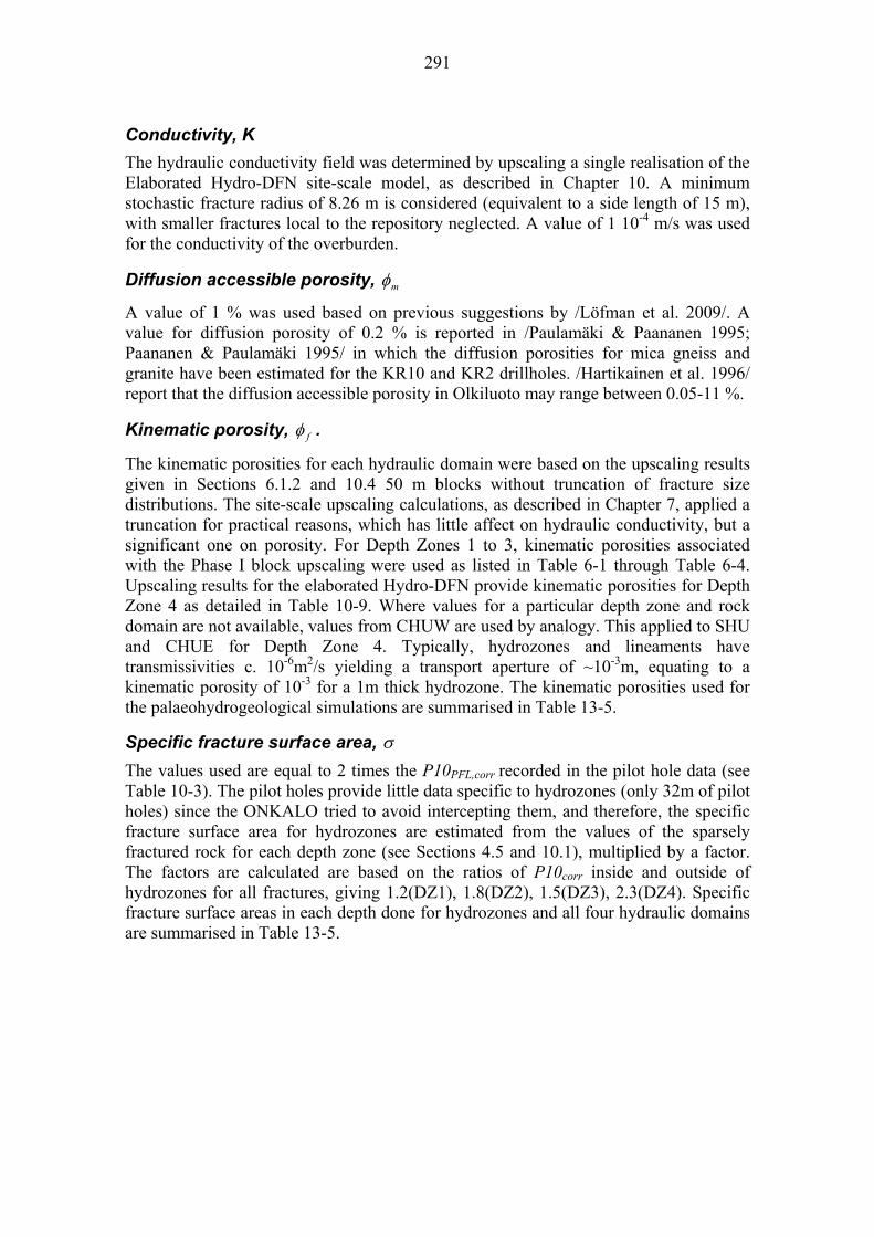
291
Conductivity, K
The hydraulic conductivity field was determined by upscaling a single realisation of the Elaborated Hydro-DFN site-scale model, as described in Chapter 10. A minimum stochastic fracture radius of 8.26 m is considered (equivalent to a side length of 15 m), with smaller fractures local to the repository neglected. A value of 1 10-4 m/s was used for the conductivity of the overburden.
Diffusion accessible porosity, m
A value of 1 % was used based on previous suggestions by /Löfman et al. 2009/. A value for diffusion porosity of 0.2 % is reported in /Paulamäki & Paananen 1995; Paananen & Paulamäki 1995/ in which the diffusion porosities for mica gneiss and granite have been estimated for the KR10 and KR2 drillholes. /Hartikainen et al. 1996/ report that the diffusion accessible porosity in Olkiluoto may range between 0.05-11 %.
Kinematic porosity, f .
The kinematic porosities for each hydraulic domain were based on the upscaling results given in Sections 6.1.2 and 10.4 50 m blocks without truncation of fracture size distributions. The site-scale upscaling calculations, as described in Chapter 7, applied a truncation for practical reasons, which has little affect on hydraulic conductivity, but a significant one on porosity. For Depth Zones 1 to 3, kinematic porosities associated with the Phase I block upscaling were used as listed in Table 6-1 through Table 6-4. Upscaling results for the elaborated Hydro-DFN provide kinematic porosities for Depth Zone 4 as detailed in Table 10-9. Where values for a particular depth zone and rock domain are not available, values from CHUW are used by analogy. This applied to SHU and CHUE for Depth Zone 4. Typically, hydrozones and lineaments have transmissivities c. 10-6m2/s yielding a transport aperture of ~10-3m, equating to a kinematic porosity of 10-3 for a 1m thick hydrozone. The kinematic porosities used for the palaeohydrogeological simulations are summarised in Table 13-5.
Specific fracture surface area,
The values used are equal to 2 times the P10PFL,corr recorded in the pilot hole data (see Table 10-3). The pilot holes provide little data specific to hydrozones (only 32m of pilot holes) since the ONKALO tried to avoid intercepting them, and therefore, the specific fracture surface area for hydrozones are estimated from the values of the sparsely fractured rock for each depth zone (see Sections 4.5 and 10.1), multiplied by a factor. The factors are calculated are based on the ratios of P10corr inside and outside of hydrozones for all fractures, giving 1.2(DZ1), 1.8(DZ2), 1.5(DZ3), 2.3(DZ4). Specific fracture surface areas in each depth done for hydrozones and all four hydraulic domains are summarised in Table 13-5.

292
Table 13-5. Kinematic porosity and specific fracture surface area, , used in the base case model, for each hydraulic domain and depth zone.
Domain Depth Zone Kinematic Porosity (m-1)
NHU DZ1 2.2E-04 3.238
NHU DZ2 6.8E-05 0.692
NHU DZ3 3.5E-05 0.698
NHU DZ4 1.3E-05 0.372
CHUW DZ1 1.9E-04 3.238
CHUW DZ2 6.6E-05 0.692
CHUW DZ3 4.1E-05 0.698
CHUW DZ4 1.4E-05 0.372
CHUE DZ1 2.1E-04 3.238
CHUE DZ2 5.4E-05 0.692
CHUE DZ3 3.1E-05 0.698
CHUE DZ4 1.4E-05 0.372
SHU DZ1 2.0E-04 3.238
SHU DZ2 5.9E-05 0.692
SHU DZ3 1.9E-05 0.698
SHU DZ4 1.4E-05 0.372
HZ DZ1 1.0E-03 3.732
HZ DZ2 1.0E-03 1.255
HZ DZ3 1.0E-03 1.059
HZ DZ4 1.0E-03 0.863
Molecular diffusivity, mD
A value of 10-9 m2/s was used, as consistent with /Löfman et al. 2009/.
Effective diffusion coefficient, iD
A value of 10-13 m2/s was used, as consistent with /Löfman et al. 2009/.
Longitudinal dispersion length, L , and transverse dispersion length, T
The longitudinal dispersion length used was 30.0m and the transverse dispersion length used was 10.0m for all rock domains and depth zones.
Tortuosity,
A value of 1 was used for all rock domains and depth zones.
Diffusion length, d
The diffusion length used was related to the specific fracture surface area according to the relation:
1
d (13-12)
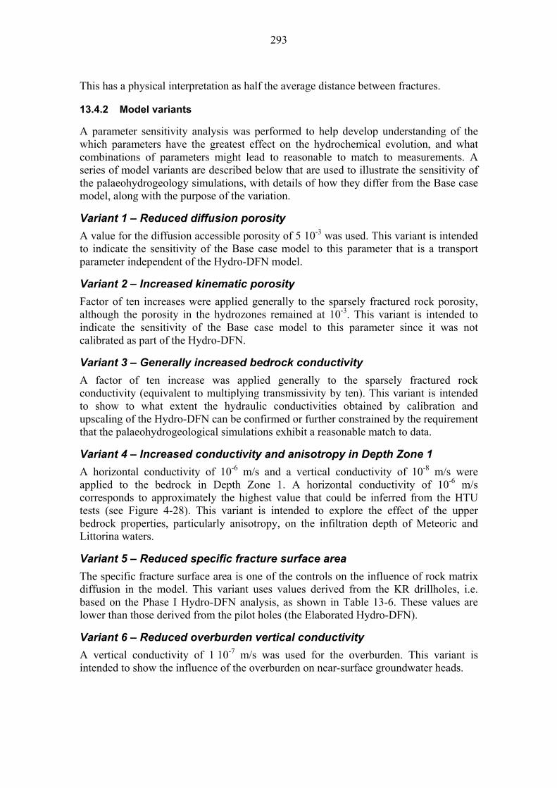
293
This has a physical interpretation as half the average distance between fractures.
13.4.2 Model variants
A parameter sensitivity analysis was performed to help develop understanding of the which parameters have the greatest effect on the hydrochemical evolution, and what combinations of parameters might lead to reasonable to match to measurements. A series of model variants are described below that are used to illustrate the sensitivity of the palaeohydrogeology simulations, with details of how they differ from the Base case model, along with the purpose of the variation.
Variant 1 – Reduced diffusion porosity
A value for the diffusion accessible porosity of 5 10-3 was used. This variant is intended to indicate the sensitivity of the Base case model to this parameter that is a transport parameter independent of the Hydro-DFN model.
Variant 2 – Increased kinematic porosity
Factor of ten increases were applied generally to the sparsely fractured rock porosity, although the porosity in the hydrozones remained at 10-3. This variant is intended to indicate the sensitivity of the Base case model to this parameter since it was not calibrated as part of the Hydro-DFN.
Variant 3 – Generally increased bedrock conductivity
A factor of ten increase was applied generally to the sparsely fractured rock conductivity (equivalent to multiplying transmissivity by ten). This variant is intended to show to what extent the hydraulic conductivities obtained by calibration and upscaling of the Hydro-DFN can be confirmed or further constrained by the requirement that the palaeohydrogeological simulations exhibit a reasonable match to data.
Variant 4 – Increased conductivity and anisotropy in Depth Zone 1
A horizontal conductivity of 10-6 m/s and a vertical conductivity of 10-8 m/s were applied to the bedrock in Depth Zone 1. A horizontal conductivity of 10-6 m/s corresponds to approximately the highest value that could be inferred from the HTU tests (see Figure 4-28). This variant is intended to explore the effect of the upper bedrock properties, particularly anisotropy, on the infiltration depth of Meteoric and Littorina waters.
Variant 5 – Reduced specific fracture surface area
The specific fracture surface area is one of the controls on the influence of rock matrix diffusion in the model. This variant uses values derived from the KR drillholes, i.e. based on the Phase I Hydro-DFN analysis, as shown in Table 13-6. These values are lower than those derived from the pilot holes (the Elaborated Hydro-DFN).
Variant 6 – Reduced overburden vertical conductivity
A vertical conductivity of 1 10-7 m/s was used for the overburden. This variant is intended to show the influence of the overburden on near-surface groundwater heads.
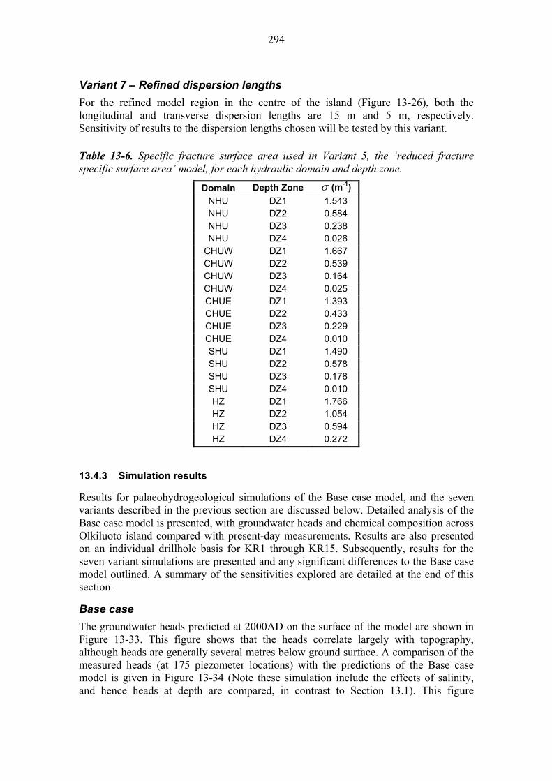
294
Variant 7 – Refined dispersion lengths
For the refined model region in the centre of the island (Figure 13-26), both the longitudinal and transverse dispersion lengths are 15 m and 5 m, respectively. Sensitivity of results to the dispersion lengths chosen will be tested by this variant.
Table 13-6. Specific fracture surface area used in Variant 5, the ‘reduced fracture specific surface area’ model, for each hydraulic domain and depth zone.
Domain Depth Zone (m-1)
NHU DZ1 1.543 NHU DZ2 0.584 NHU DZ3 0.238 NHU DZ4 0.026
CHUW DZ1 1.667 CHUW DZ2 0.539 CHUW DZ3 0.164 CHUW DZ4 0.025 CHUE DZ1 1.393 CHUE DZ2 0.433 CHUE DZ3 0.229 CHUE DZ4 0.010 SHU DZ1 1.490 SHU DZ2 0.578 SHU DZ3 0.178 SHU DZ4 0.010 HZ DZ1 1.766 HZ DZ2 1.054 HZ DZ3 0.594 HZ DZ4 0.272
13.4.3 Simulation results
Results for palaeohydrogeological simulations of the Base case model, and the seven variants described in the previous section are discussed below. Detailed analysis of the Base case model is presented, with groundwater heads and chemical composition across Olkiluoto island compared with present-day measurements. Results are also presented on an individual drillhole basis for KR1 through KR15. Subsequently, results for the seven variant simulations are presented and any significant differences to the Base case model outlined. A summary of the sensitivities explored are detailed at the end of this section.
Base case
The groundwater heads predicted at 2000AD on the surface of the model are shown in Figure 13-33. This figure shows that the heads correlate largely with topography, although heads are generally several metres below ground surface. A comparison of the measured heads (at 175 piezometer locations) with the predictions of the Base case model is given in Figure 13-34 (Note these simulation include the effects of salinity, and hence heads at depth are compared, in contrast to Section 13.1). This figure
295
suggests a reasonable agreement. The average error is 0.25 m and the average absolute error is 0.83 m. The model slightly over-predicts the heads in low-lying drillhole KR3 with an average error of 1.4 m, and does not reproduce the heads above 7m seen in some drillholes, e.g. KR04. This may be due to regions of tighter overburden, i.e. heterogeneity of the soil properties that are not considered here. A comparison of modelled and measured heads for specific drillholes are shown in Figure 13-35 and Figure 13-36, with the largest discrepancies seen in KR3 and KR8.
The head predictions are quite sensitive to the properties of the overburden, as discussed in the section concerning Variant 6. The overburden is represented simply in these models, with homogeneous hydraulic properties but variable depth throughout the domain. A better fit to the near surface head data might require a more elaborate model of the overburden and consideration of the unsaturated zone. In /Karvonen 2011/ the coupling of surface hydrological (SHYD) and bedrock groundwater flow (FEFTRA) models was implemented with some success in matching the near surface head measurements, although it is noted that KR04 was also under-estimated.
It is significant that a reasonable match to baseline heads was achieved here in the Base Case model without implementing any of the changes suggested in Table 13-1. This is thought to be due to the inclusion of the overburden with appropriate properties and a recharge boundary condition reducing the infiltration to the hydrozones and sparsely fractured rock. This results in a lowering of heads in the bedrock without having to increase the transmissivity of the near-surface bedrock. Hence, this indicates there are alternative explanations of the observed distributions of heads in the bedrock relating to uncertainties on the order of a factor 2-3 in the effective bulk properties of the overburden and near-surface bedrock. However, since several drillholes suggest significant vertical gradients in the top 50 m, it suggests any adjustments made to better calibrate with head measurements be focussed on the properties of the overburden or top 50 m of bedrock.
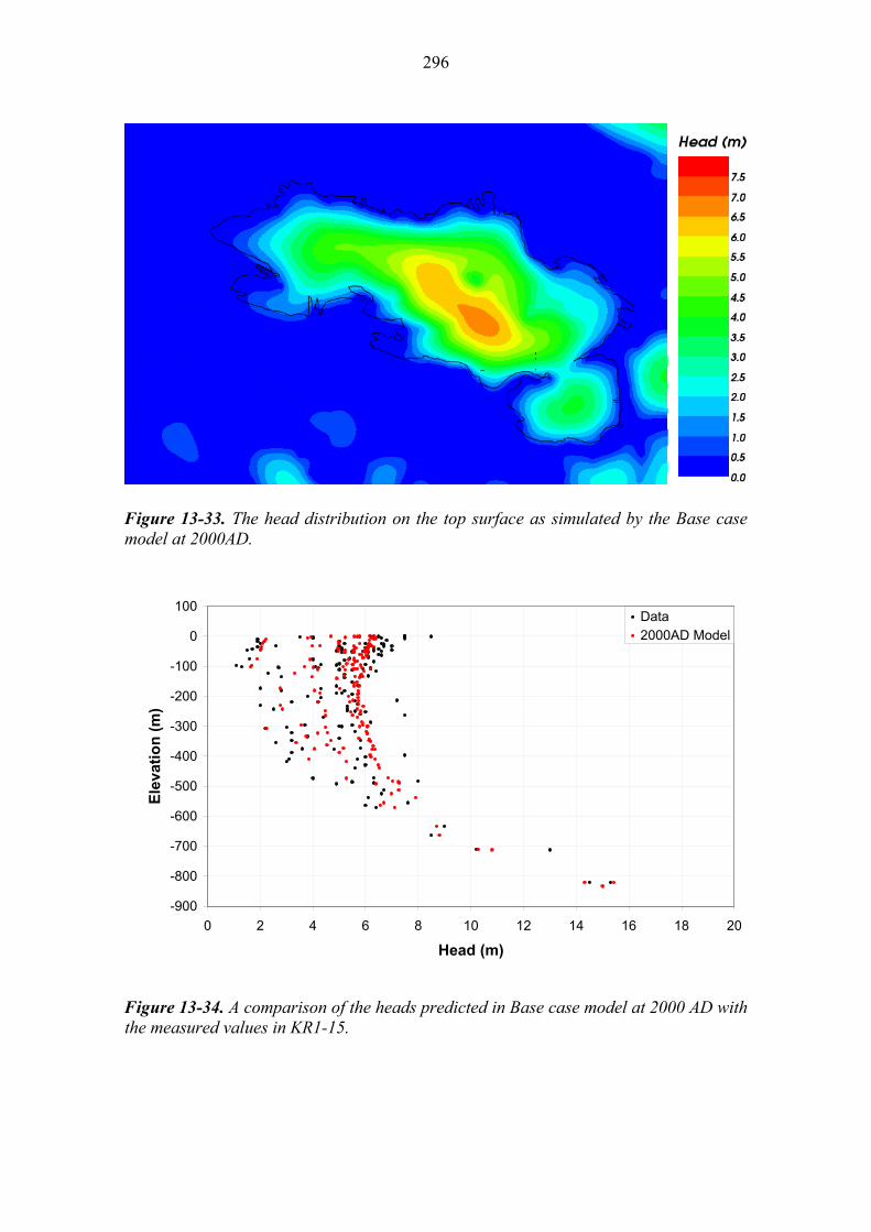
296
Figure 13-33. The head distribution on the top surface as simulated by the Base case model at 2000AD.
-900
-800
-700
-600
-500
-400
-300
-200
-100
0
100
0 2 4 6 8 10 12 14 16 18 20
Head (m)
Ele
vati
on
(m
)
Data2000AD Model
Figure 13-34. A comparison of the heads predicted in Base case model at 2000 AD with the measured values in KR1-15.
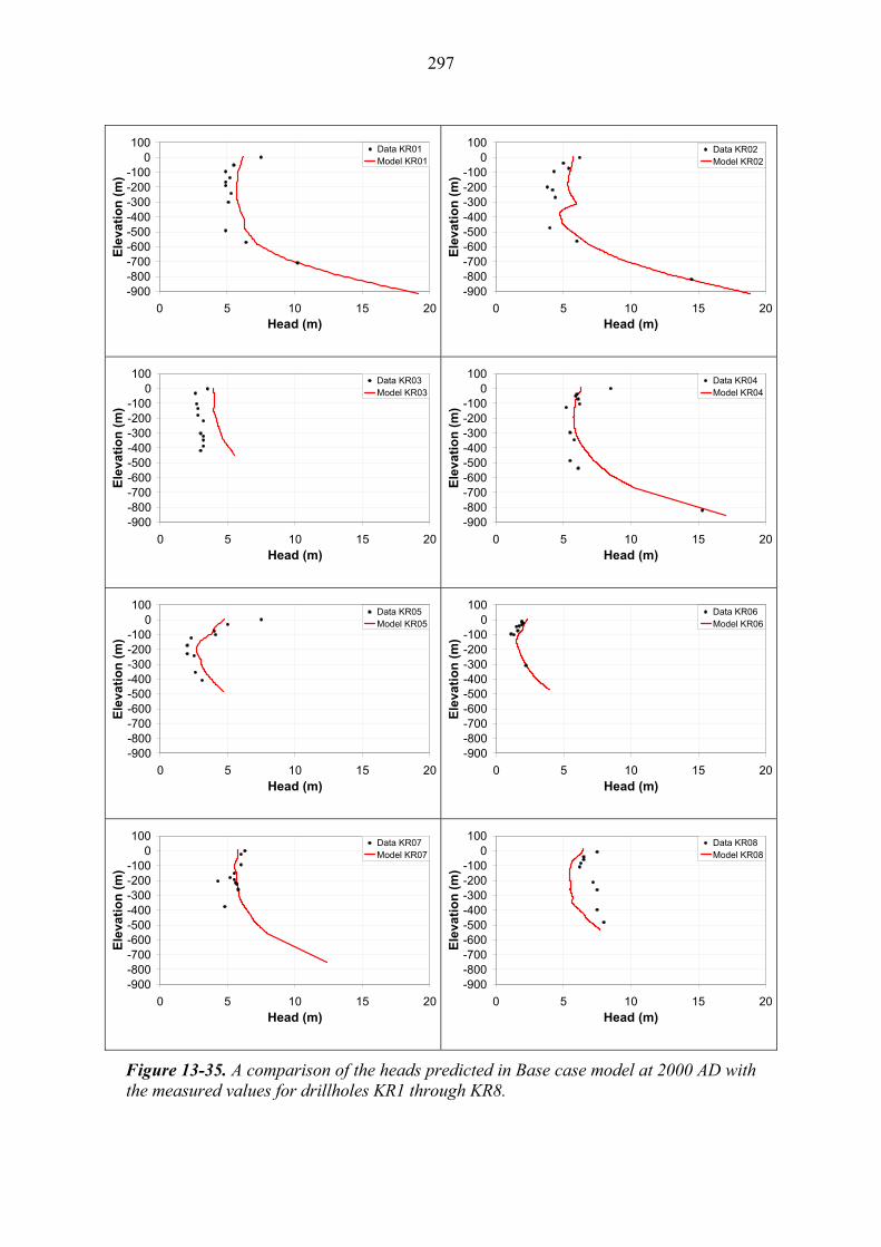
297
-900-800-700-600-500-400-300-200-100
0100
0 5 10 15 20Head (m)
Ele
vati
on
(m
)
Data KR01Model KR01
-900-800-700-600-500-400-300-200-100
0100
0 5 10 15 20Head (m)
Ele
vati
on
(m
)
Data KR02Model KR02
-900-800-700-600-500-400-300-200-100
0100
0 5 10 15 20Head (m)
Ele
vati
on
(m
)
Data KR03Model KR03
-900-800-700-600-500-400-300-200-100
0100
0 5 10 15 20Head (m)
Ele
vati
on
(m
)
Data KR04Model KR04
-900-800-700-600-500-400-300-200-100
0100
0 5 10 15 20Head (m)
Ele
vati
on
(m
)
Data KR05Model KR05
-900-800-700-600-500-400-300-200-100
0100
0 5 10 15 20Head (m)
Ele
vati
on
(m
)
Data KR06Model KR06
-900-800-700-600-500-400-300-200-100
0100
0 5 10 15 20Head (m)
Ele
vati
on
(m
)
Data KR07Model KR07
-900-800-700-600-500-400-300-200-100
0100
0 5 10 15 20Head (m)
Ele
vati
on
(m
)
Data KR08Model KR08
Figure 13-35. A comparison of the heads predicted in Base case model at 2000 AD with the measured values for drillholes KR1 through KR8.
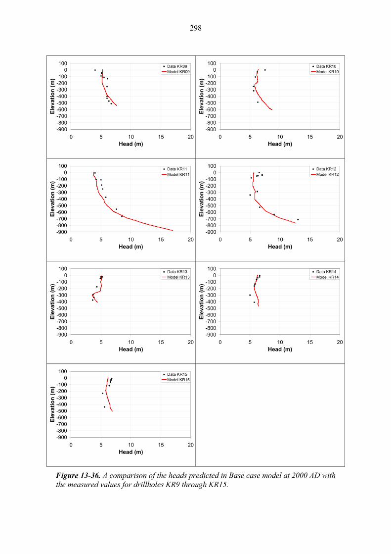
298
-900-800-700-600-500-400-300-200-100
0100
0 5 10 15 20Head (m)
Ele
vati
on
(m
)
Data KR09Model KR09
-900-800-700-600-500-400-300-200-100
0100
0 5 10 15 20Head (m)
Ele
vati
on
(m
)
Data KR10Model KR10
-900-800-700-600-500-400-300-200-100
0100
0 5 10 15 20Head (m)
Ele
vati
on
(m
)
Data KR11Model KR11
-900-800-700-600-500-400-300-200-100
0100
0 5 10 15 20Head (m)
Ele
vati
on
(m
)
Data KR12Model KR12
-900-800-700-600-500-400-300-200-100
0100
0 5 10 15 20Head (m)
Ele
vati
on
(m
)
Data KR13Model KR13
-900-800-700-600-500-400-300-200-100
0100
0 5 10 15 20Head (m)
Ele
vati
on
(m
)
Data KR14Model KR14
-900-800-700-600-500-400-300-200-100
0100
0 5 10 15 20Head (m)
Ele
vati
on
(m
)
Data KR15Model KR15
Figure 13-36. A comparison of the heads predicted in Base case model at 2000 AD with the measured values for drillholes KR9 through KR15.

299
A qualitative description of the predictions for the evolution of groundwater composition for the Base case model is given below.
The mass fraction of Brine predicted at 2000AD in the fracture water is shown in Figure 13-37. The distribution of this reference water at depth is substantially unchanged from the supplied initial condition. This is a consequence of the high density of this reference water, combined with its location at depth where low flow rates are expected. The distribution remains stratified by depth, with relatively minor perturbations around this trend.
The mass fraction of Subglacial water predicted at 2000AD in the fractures is shown in Figure 13-38. The only source of this reference water is the assumed initial condition, where Subglacial water, along with Brine, is present in the rock matrix and fractures. The Subglacial water is predicted to be present at mass fractions c. 0.5 around elevations between -300 m to -800 m at 2000AD. Above this elevation, this reference water has been displaced by Littorina and Meteoric waters. Below this elevation Brine is dominant. The influence of hydrozones is apparent in Figure 13-38, where their presence allows Littorina and Meteoric waters to displace the Subglacial water to a greater extent than in the sparsely fractured rock.
The mass fraction of Glacial water predicted in the fractures is shown in Figure 13-39. The only source of this reference water is the assumed initial condition, where Glacial water, along with Brine and Subglacial water, is present in the rock fractures and matrix. At 6000 BC the figure shows the initial condition. By 2000AD the Glacial water is predicted to be present at reduced mass fractions at elevations down to -800m. The influence of hydrozones is apparent, where their presence allows Littorina and Meteoric waters to displace the Glacial water to a greater extent than in the sparsely fractured rock.
The mass fraction of Littorina water predicted in the fractures is shown in Figure 13-40. The source of this reference water is the Littorina and Baltic Seas, before the Olkiluoto Island rises above sea level. At 2000 BC, before the emergence of Olkiluoto above sea level, the figure shows mass fractions of around 0.5 at elevations of approximately -300 m. Hydrozones have allowed the Littorina to infiltrate to greater depth in some areas. By 2000AD the Littorina water is predicted to have been displaced below Olkiluoto Island to an elevation of approximately -150 m.
The mass fraction of Meteoric water predicted in the fractures is shown in Figure 13-41. At 0AD the Olkiluoto island has only just started to emerge from the sea, and so minimal Meteoric water has infiltrated, with mass fractions of 0.3 down to elevations of c. -40 m. By 2000AD Meteoric water becomes the dominant reference water in the top 100 m of bedrock, with values greater than 0.8 predicted down to elevations around -150 m.
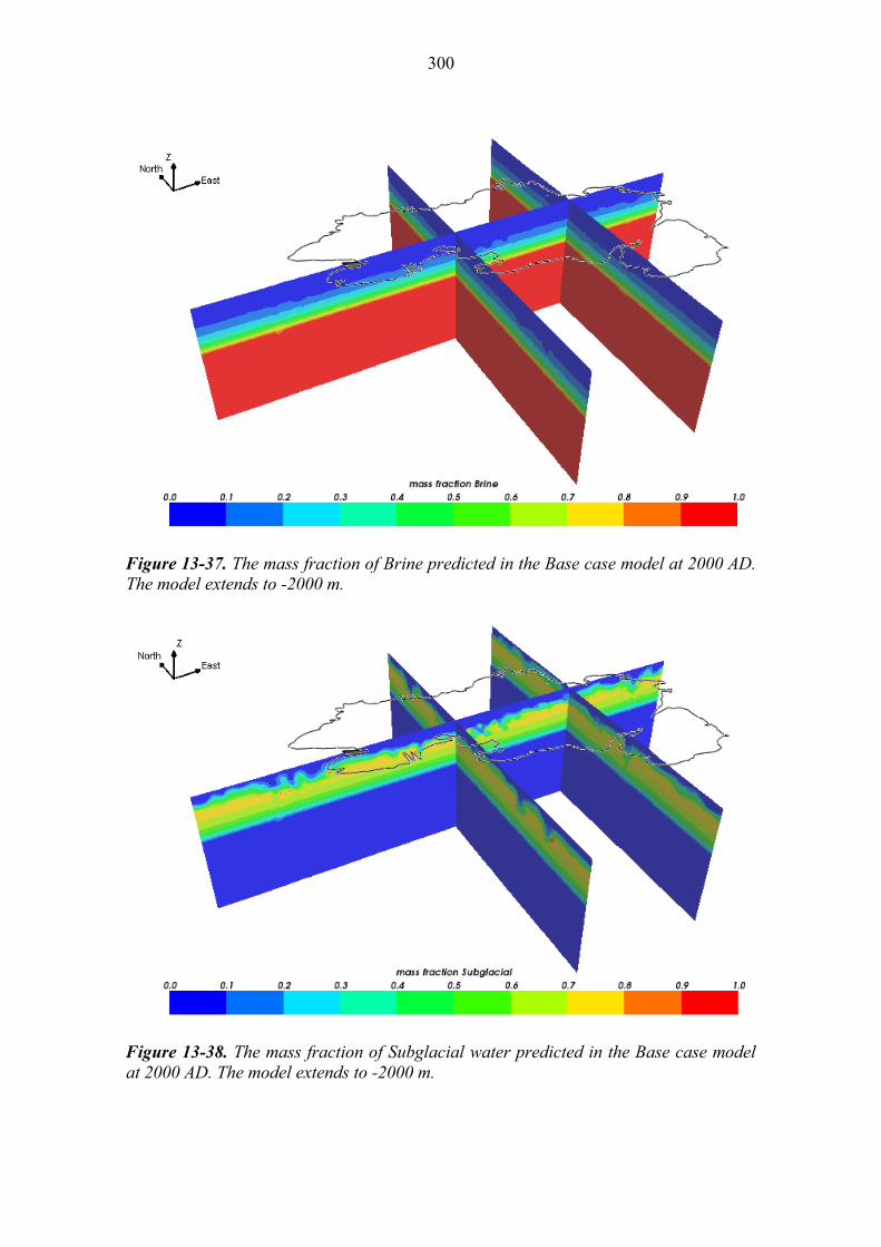
300
Figure 13-37. The mass fraction of Brine predicted in the Base case model at 2000 AD. The model extends to -2000 m.
Figure 13-38. The mass fraction of Subglacial water predicted in the Base case model at 2000 AD. The model extends to -2000 m.
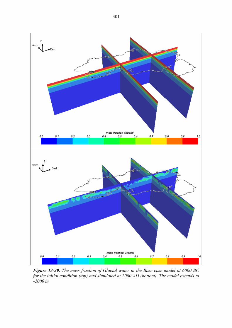
301
Figure 13-39. The mass fraction of Glacial water in the Base case model at 6000 BC for the initial condition (top) and simulated at 2000 AD (bottom). The model extends to -2000 m.

302
Figure 13-40. The mass fraction of Littorina water predicted in the Base case model at 2000 BC (top) and 2000 AD (bottom). The model extends to -2000 m.

303
Figure 13-41. The mass fraction of Meteoric water predicted in the Base case model at 0 AD (top) and 2000 AD (bottom). The model extends to -2000 m.

304
A series of comparisons between the measured concentrations of various chemicals in the fracture water and the predictions of the Base case model are shown in Figure 13-42 through Figure 13-51. These comparisons present the results by elevation. The impacts of hydrozones on the simulations are considered later.
Figure 13-42 and Figure 13-43 show Cl and Br concentrations respectively. These chemicals are characteristic of the Brine, and to a lesser extent Littorina, reference waters. Below approximately –500 m the predicted concentrations do not deviate significantly from the supplied initial condition. Above around –100 m the model accurately predicts low concentrations of Cl and Br, as the Brine has been displaced by Meteoric water. The model partially simulates the increased Cl and Br concentrations between –100 m and –300 m. The simulations are reasonable for Br in the region, but under-predict Cl relative to some measurement points. These points with lower Br/Cl ratios are indicative of salinity of Littorina water origin.
Figure 13-44 shows a comparison of the predicted SO4 concentrations with the measured data, which is an indicator of Littorina or marine origin waters. The data suggests Littorina water has infiltrated to give elevated SO4 concentrations at elevations between –100 m and –300 m. The model partially reproduces this pattern, although the peak of the elevated concentrations is shifted down to c. –300 m. Above around –150 m much of the Littorina water is predicted to have been displaced by Meteoric water, as indicated by HCO3 shown in Figure 13-45. This figure suggests that the model is slightly over-predicting the depth to which the Meteoric water has infiltrated. A series of comparisons for individual drillholes in terms of the predicted and measured values of SO4 and HCO3 in the fracture water are shown in Figure 13-46 and Figure 13-48, respectively. Some drillhole comparisons are better than others suggesting that SO4
concentrations suggesting that the hydraulic conductivity in the model might be too high in places. The sensitivity of predicted SO4 concentrations to uncertain hydraulic properties in the hydrozones and sparsely fracture rock is explored by a series of stochastic realisations and presented in Figure 13-64.
Figure 13-50 and Figure 13-51 show a comparison between the predictions of the Base case model and measured data for δ2H and δ18O, respectively, in the fracture water. Low δ2H and δ18O values are characteristic of Glacial water. Both graphs suggest that the model is slightly over-predicting the fraction of Glacial water below approximately -200 m. There is little change from the initial condition below -400 m. The simulations appear to contain less variability below -300 m in these environmental isotopes compared to the measurements, which is probably due to the simplification of using an initial condition without lateral variation. In reality the initial conditions may have been different between hydrozones and the sparsely fractured rock, for example. This may be a result of the deterministic description of the hydrozones used in the base case, and can be explored by considering more realisations with heterogeneous hydrozones.
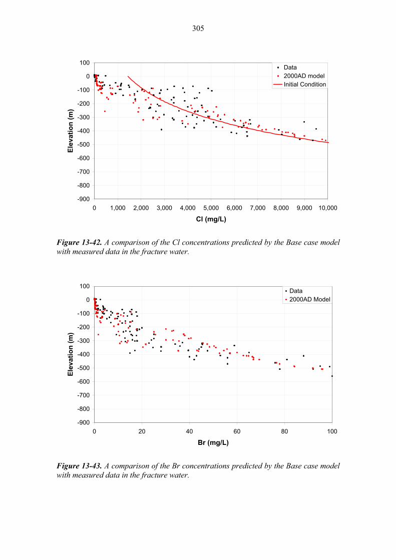
305
-900
-800
-700
-600
-500
-400
-300
-200
-100
0
100
0 1,000 2,000 3,000 4,000 5,000 6,000 7,000 8,000 9,000 10,000
Cl (mg/L)
Ele
vati
on
(m
)Data2000AD modelInitial Condition
Figure 13-42. A comparison of the Cl concentrations predicted by the Base case model with measured data in the fracture water.
-900
-800
-700
-600
-500
-400
-300
-200
-100
0
100
0 20 40 60 80 100
Br (mg/L)
Ele
vati
on
(m
)
Data2000AD Model
Figure 13-43. A comparison of the Br concentrations predicted by the Base case model with measured data in the fracture water.

306
-900
-800
-700
-600
-500
-400
-300
-200
-100
0
100
0 100 200 300 400 500 600
SO4 (mg/L)
Ele
vati
on
(m
)Data2000AD Model
Figure 13-44. A comparison of the SO4 concentrations predicted by the Base case model with measured data in the fracture water.
-900
-800
-700
-600
-500
-400
-300
-200
-100
0
100
0 100 200 300 400 500 600
HCO3 (mg/L)
Ele
vati
on
(m
)
Data2000AD Model
Figure 13-45. A comparison of the HCO3 concentrations predicted by the Base case model with measured data in the fracture water.

307
-900-800-700-600-500-400-300-200-100
0100
0 100 200 300 400 500 600SO4 (mg/L)
Ele
vati
on
(m
)
Data KR01Model KR01
-900-800-700-600-500-400-300-200-100
0100
0 100 200 300 400 500 600SO4 (mg/L)
Ele
vati
on
(m
)
Data KR02Model KR02
-900-800-700-600-500-400-300-200-100
0100
0 100 200 300 400 500 600SO4 (mg/L)
Ele
vati
on
(m
)
Data KR03Model KR03
-900-800-700-600-500-400-300-200-100
0100
0 100 200 300 400 500 600SO4 (mg/L)
Ele
vati
on
(m
)
Data KR04Model KR04
-900-800-700-600-500-400-300-200-100
0100
0 100 200 300 400 500 600SO4 (mg/L)
Ele
vati
on
(m
)
Data KR05Model KR05
-900-800-700-600-500-400-300-200-100
0100
0 100 200 300 400 500 600SO4 (mg/L)
Ele
vati
on
(m
)
Data KR06Model KR06
-900-800-700-600-500-400-300-200-100
0100
0 100 200 300 400 500 600SO4 (mg/L)
Ele
vati
on
(m
)
Data KR07Model KR07
-900-800-700-600-500-400-300-200-100
0100
0 100 200 300 400 500 600SO4 (mg/L)
Ele
vati
on
(m
)
Data KR08Model KR08
Figure 13-46. A comparison of the SO4 concentrations predicted by the Base case model with measured data in the fracture water for drillholes KR1 through KR8.
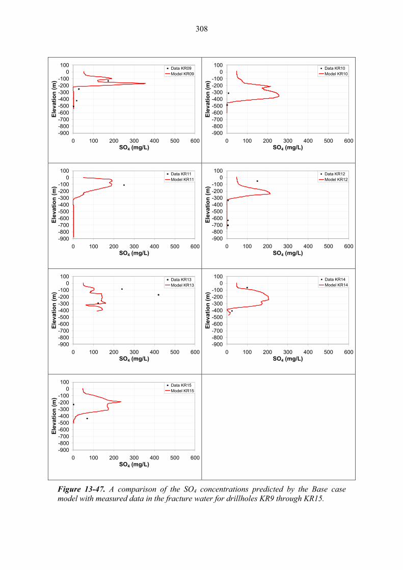
308
-900-800-700-600-500-400-300-200-100
0100
0 100 200 300 400 500 600SO4 (mg/L)
Ele
vati
on
(m
)
Data KR09Model KR09
-900-800-700-600-500-400-300-200-100
0100
0 100 200 300 400 500 600SO4 (mg/L)
Ele
vati
on
(m
)
Data KR10Model KR10
-900-800-700-600-500-400-300-200-100
0100
0 100 200 300 400 500 600SO4 (mg/L)
Ele
vati
on
(m
)
Data KR11Model KR11
-900-800-700-600-500-400-300-200-100
0100
0 100 200 300 400 500 600SO4 (mg/L)
Ele
vati
on
(m
)
Data KR12Model KR12
-900-800-700-600-500-400-300-200-100
0100
0 100 200 300 400 500 600SO4 (mg/L)
Ele
vati
on
(m
)
Data KR13Model KR13
-900-800-700-600-500-400-300-200-100
0100
0 100 200 300 400 500 600SO4 (mg/L)
Ele
vati
on
(m
)
Data KR14Model KR14
-900-800-700-600-500-400-300-200-100
0100
0 100 200 300 400 500 600SO4 (mg/L)
Ele
vati
on
(m
)
Data KR15Model KR15
Figure 13-47. A comparison of the SO4 concentrations predicted by the Base case model with measured data in the fracture water for drillholes KR9 through KR15.
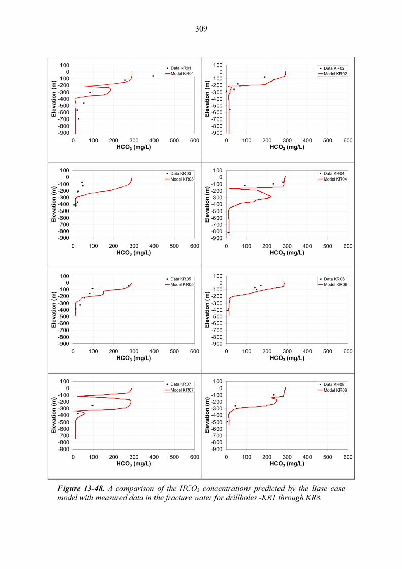
309
-900-800-700-600-500-400-300-200-100
0100
0 100 200 300 400 500 600HCO3 (mg/L)
Ele
vati
on
(m
)
Data KR01Model KR01
-900-800-700-600-500-400-300-200-100
0100
0 100 200 300 400 500 600HCO3 (mg/L)
Ele
vati
on
(m
)
Data KR02Model KR02
-900-800-700-600-500-400-300-200-100
0100
0 100 200 300 400 500 600HCO3 (mg/L)
Ele
vati
on
(m
)
Data KR03Model KR03
-900-800-700-600-500-400-300-200-100
0100
0 100 200 300 400 500 600HCO3 (mg/L)
Ele
vati
on
(m
)
Data KR04Model KR04
-900-800-700-600-500-400-300-200-100
0100
0 100 200 300 400 500 600HCO3 (mg/L)
Ele
vati
on
(m
)
Data KR05Model KR05
-900-800-700-600-500-400-300-200-100
0100
0 100 200 300 400 500 600HCO3 (mg/L)
Ele
vati
on
(m
)
Data KR06Model KR06
-900-800-700-600-500-400-300-200-100
0100
0 100 200 300 400 500 600HCO3 (mg/L)
Ele
vati
on
(m
)
Data KR07Model KR07
-900-800-700-600-500-400-300-200-100
0100
0 100 200 300 400 500 600HCO3 (mg/L)
Ele
vati
on
(m
)
Data KR08Model KR08
Figure 13-48. A comparison of the HCO3 concentrations predicted by the Base case model with measured data in the fracture water for drillholes -KR1 through KR8.
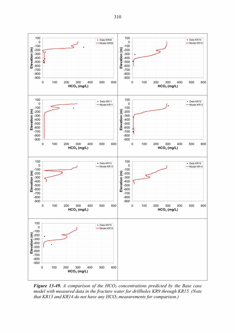
310
-900-800-700-600-500-400-300-200-100
0100
0 100 200 300 400 500 600HCO3 (mg/L)
Ele
vati
on
(m
)
Data KR09Model KR09
-900-800-700-600-500-400-300-200-100
0100
0 100 200 300 400 500 600HCO3 (mg/L)
Ele
vati
on
(m
)
Data KR10Model KR10
-900-800-700-600-500-400-300-200-100
0100
0 100 200 300 400 500 600HCO3 (mg/L)
Ele
vati
on
(m
)
Data KR11Model KR11
-900-800-700-600-500-400-300-200-100
0100
0 100 200 300 400 500 600HCO3 (mg/L)
Ele
vati
on
(m
)
Data KR12Model KR12
-900-800-700-600-500-400-300-200-100
0100
0 100 200 300 400 500 600HCO3 (mg/L)
Ele
vati
on
(m
)
Data KR13Model KR13
-900-800-700-600-500-400-300-200-100
0100
0 100 200 300 400 500 600HCO3 (mg/L)
Ele
vati
on
(m
)
Data KR14Model KR14
-900-800-700-600-500-400-300-200-100
0100
0 100 200 300 400 500 600HCO3 (mg/L)
Ele
vati
on
(m
)
Data KR15Model KR15
Figure 13-49. A comparison of the HCO3 concentrations predicted by the Base case model with measured data in the fracture water for drillholes KR9 through KR15. (Note that KR13 and KR14 do not have any HCO3 measurements for comparison.)

311
-900
-800
-700
-600
-500
-400
-300
-200
-100
0
100
-150 -125 -100 -75 -50
H2 (0/00 VSMOW)
Ele
vati
on
(m
)
Data2000 AD Model
Figure 13-50. A comparison of the δ2H distribution predicted by the Base case model with measured data in the fracture water.
-900
-800
-700
-600
-500
-400
-300
-200
-100
0
100
-20 -15 -10 -5 0
d18O (0/00 VSMOW)
Ele
vati
on
(m
)
Data2000AD Model
Figure 13-51. A comparison of the δ18O distribution predicted by the Base case model with measured data in the fracture water.

312
The graphs above indicate the overall match to the chemistry data with depth. The influence of hydrozones, as predicted by the Base case model, is considered below. Figure 13-52 illustrates how the presence of the hydrozones is predicted to change the Littorina mass fraction, compared to the sparsely fractured rock, at -275 m. The bounding lineaments have a strong localised influence on the Littorina mass fraction, but there are no sampling locations near the lineaments to compare to predictions. Hydrozones HZ20A, HZ20B, HZ21B, BFZ100, HZ001 and HZ099 also have a significant affect on the local Littorina concentration fractions. Such an effect is not readily apparent in the measured data; see for example in Figure 13-25.
Meteoric water concentration fractions at -275m are shown in Figure 13-53. Elevated Meteoric mass fractions are apparent around HZ20A, HZ20B and BFZ100. The Base case model over-predicts the depth of infiltration of Meteoric waters, as demonstrated in Figure 13-45. Figure 13-53 suggests that some of this over-prediction is controlled by the properties hydrozones in the centre of the island.
Next we discuss the results of the parameter sensitivity variants described in Section 13.4.2.
Variant 1 – Reduced diffusion porosity
Above approximately -300 m the model is relatively insensitive to the change in this parameter. The infiltration depth of HCO3 increases slightly, by approximately 50 m, compared to the Base case.
Variant 2 – Increased kinematic porosity
The Base case model is very insensitive to changes in this parameter.
Variant 3 – Increased bedrock conductivity
The groundwater heads are reduced in the near surface, and there is less variability between the predicted heads with drillhole location. The model significantly under-predicts the vertical head gradient in the top 50m of bedrock. These results are illustrated in Figure 13-54. It is possible that making compensating changes to the hydraulic properties of the overburden could improve the match.
This model variant predicts infiltration of Meteoric water to approximately 100 m greater depth than in the Base case. Because of this there is also less Littorina water remaining at 2000 AD. The results are therefore less consistent with data.
This sensitivity suggests that the Hydro-DFN description of the sparsely fractured rock and hydrozones derived in this study provides a reasonable basis for description of bulk hydraulic properties and flow-rates at the site.
Variant 4 – Increased conductivity and anisotropy in Depth Zone 1
This change has the effect of reducing the groundwater heads in the near surface, and increasing the vertical head gradients above approximately -100 m, as shown in Figure 13-55. It is possible that making compensating changes to the hydraulic properties of the overburden could improve the match to data.
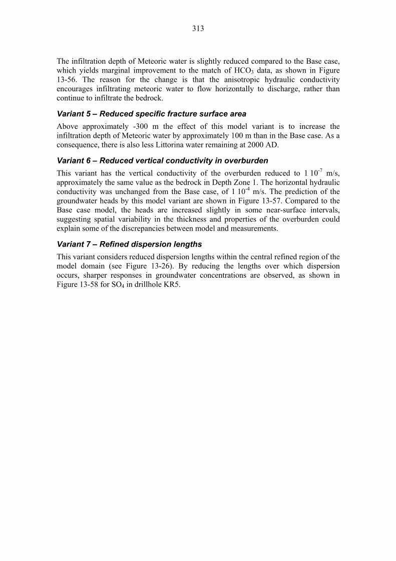
313
The infiltration depth of Meteoric water is slightly reduced compared to the Base case, which yields marginal improvement to the match of HCO3 data, as shown in Figure 13-56. The reason for the change is that the anisotropic hydraulic conductivity encourages infiltrating meteoric water to flow horizontally to discharge, rather than continue to infiltrate the bedrock.
Variant 5 – Reduced specific fracture surface area
Above approximately -300 m the effect of this model variant is to increase the infiltration depth of Meteoric water by approximately 100 m than in the Base case. As a consequence, there is also less Littorina water remaining at 2000 AD.
Variant 6 – Reduced vertical conductivity in overburden
This variant has the vertical conductivity of the overburden reduced to 1 10-7 m/s, approximately the same value as the bedrock in Depth Zone 1. The horizontal hydraulic conductivity was unchanged from the Base case, of 1 10-4 m/s. The prediction of the groundwater heads by this model variant are shown in Figure 13-57. Compared to the Base case model, the heads are increased slightly in some near-surface intervals, suggesting spatial variability in the thickness and properties of the overburden could explain some of the discrepancies between model and measurements.
Variant 7 – Refined dispersion lengths
This variant considers reduced dispersion lengths within the central refined region of the model domain (see Figure 13-26). By reducing the lengths over which dispersion occurs, sharper responses in groundwater concentrations are observed, as shown in Figure 13-58 for SO4 in drillhole KR5.
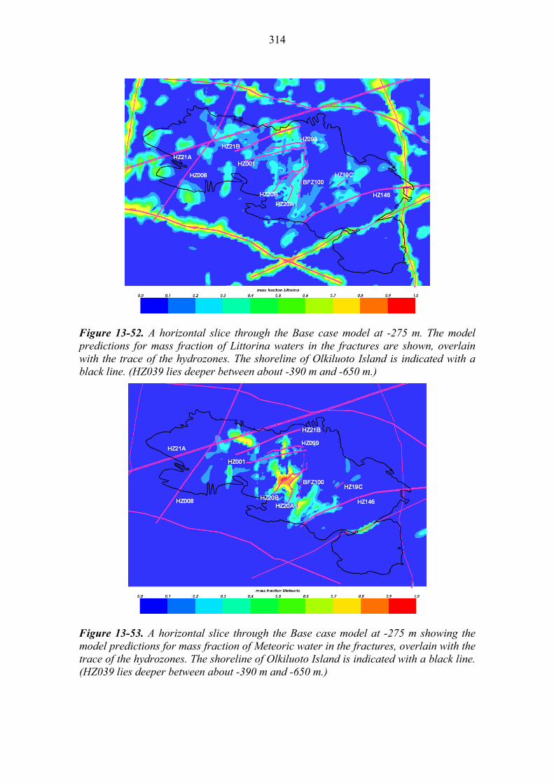
314
Figure 13-52. A horizontal slice through the Base case model at -275 m. The model predictions for mass fraction of Littorina waters in the fractures are shown, overlain with the trace of the hydrozones. The shoreline of Olkiluoto Island is indicated with a black line. (HZ039 lies deeper between about -390 m and -650 m.)
Figure 13-53. A horizontal slice through the Base case model at -275 m showing the model predictions for mass fraction of Meteoric water in the fractures, overlain with the trace of the hydrozones. The shoreline of Olkiluoto Island is indicated with a black line. (HZ039 lies deeper between about -390 m and -650 m.)
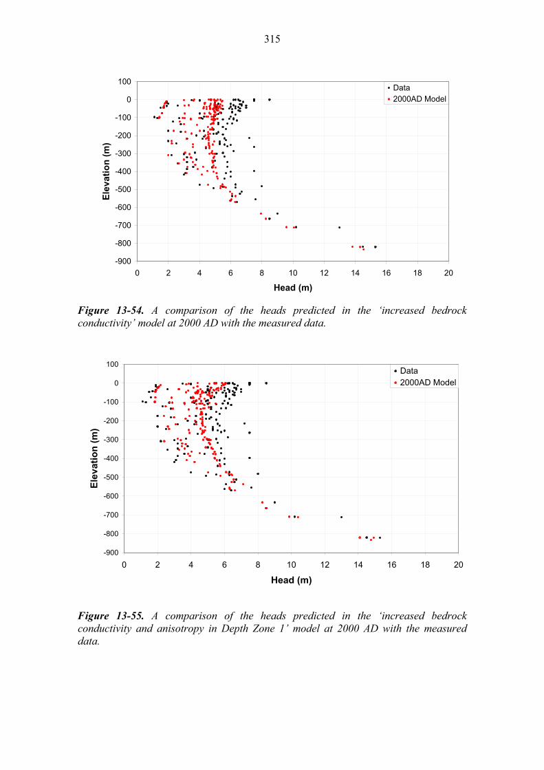
315
-900
-800
-700
-600
-500
-400
-300
-200
-100
0
100
0 2 4 6 8 10 12 14 16 18 20
Head (m)
Ele
vati
on
(m
)
Data2000AD Model
Figure 13-54. A comparison of the heads predicted in the ‘increased bedrock conductivity’ model at 2000 AD with the measured data.
-900
-800
-700
-600
-500
-400
-300
-200
-100
0
100
0 2 4 6 8 10 12 14 16 18 20
Head (m)
Ele
vati
on
(m
)
Data2000AD Model
Figure 13-55. A comparison of the heads predicted in the ‘increased bedrock conductivity and anisotropy in Depth Zone 1’ model at 2000 AD with the measured data.
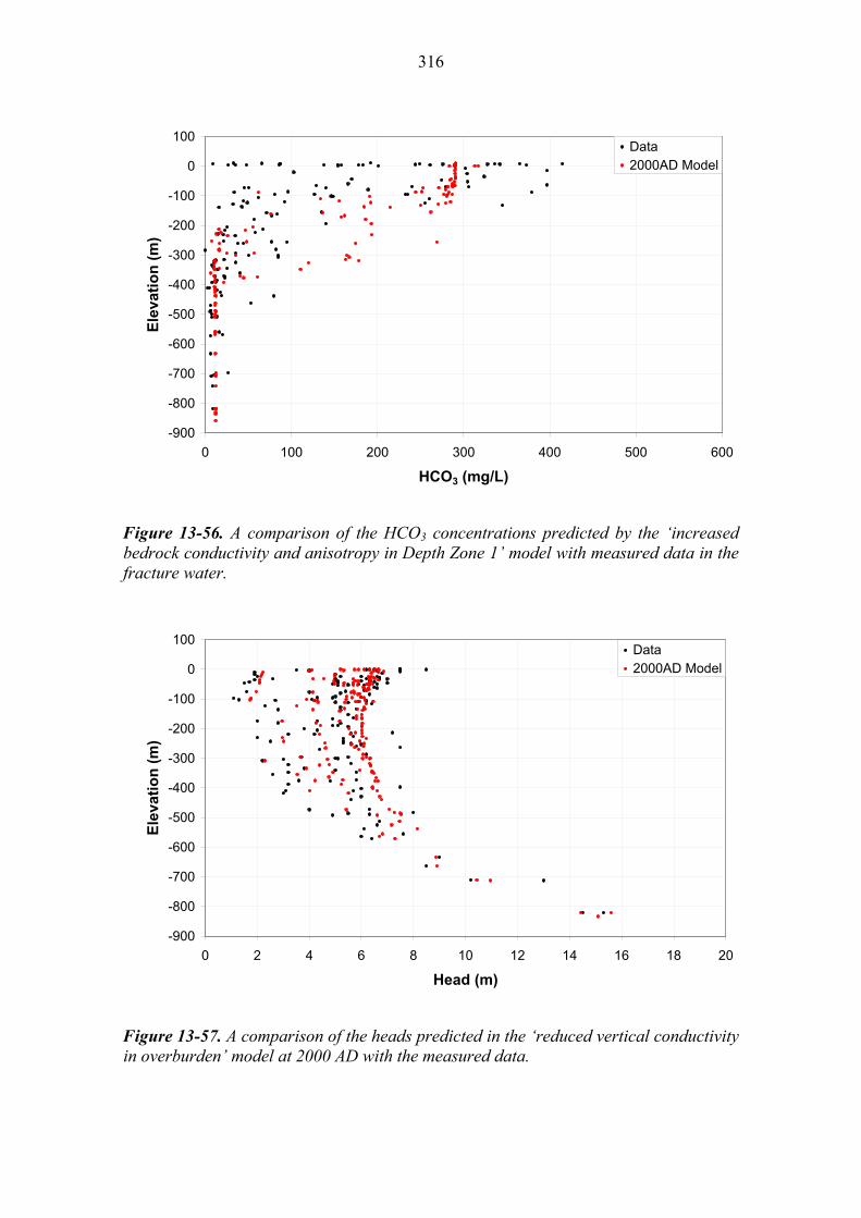
316
-900
-800
-700
-600
-500
-400
-300
-200
-100
0
100
0 100 200 300 400 500 600
HCO3 (mg/L)
Ele
vati
on
(m
)Data2000AD Model
Figure 13-56. A comparison of the HCO3 concentrations predicted by the ‘increased bedrock conductivity and anisotropy in Depth Zone 1’ model with measured data in the fracture water.
-900
-800
-700
-600
-500
-400
-300
-200
-100
0
100
0 2 4 6 8 10 12 14 16 18 20
Head (m)
Ele
vati
on
(m
)
Data2000AD Model
Figure 13-57. A comparison of the heads predicted in the ‘reduced vertical conductivity in overburden’ model at 2000 AD with the measured data.

317
-900
-800
-700
-600
-500
-400
-300
-200
-100
0
100
0 100 200 300 400 500 600
SO4 (mg/L)
Ele
vat
ion
(m
)
Data KR05
Model KR05 -900
-800
-700
-600
-500
-400
-300
-200
-100
0
100
0 100 200 300 400 500 600
SO4 (mg/L)
Ele
vati
on
(m
)Data KR05Model KR05
Figure 13-58. Groundwater concentration of SO4 predicted in drillhole KR05 by the base case model (left) and the ‘refined dispersion length’ model (right) at 2000 AD with the measured data.
13.4.4 Summary
The palaeohydrogeology simulations performed suggest that a reasonable qualitative representation of the hydrochemical evolution of Olkiluoto island can be achieved using hydraulic properties derived from the upscaled Hydro-DFN and properties for the hydrozones proposed in Section 3.7 along with parameters consistent with site data.
The model variants show that some of the key sensitivities are to near-surface processes and parameters. In particular, the groundwater heads are sensitive to the conductivity of the overburden, and the hydraulic conductivity of the bedrock in Depth Zone 1. The infiltration depth of Meteoric water is also influenced by the conductivity of the bedrock in Depth Zone 1.
Increasing the bedrock conductivity generally by a factor of ten worsens the match to the HCO3 and SO4 concentration measurements as well as generally under-predicting the head distribution, suggesting that the Hydro-DFN model provides a representative description of bulk hydraulic conductivity at depth based on its constraint by the PFL data. The models are relatively insensitive to both the diffusion porosity and the kinematic porosity. Rock matrix diffusion is a key process in modelling the hydrochemical evolution, as shown by the sensitivity of the Base case model to changes to the specific fracture surface area. Rock matrix diffusion scales with both matrix porosity and specific fracture surface area, so one might expect reducing either of these parameters (Variant 1 and Variant 5) might have similar effects. The reason reducing

318
specific fracture surface area has more of an effect may be that not only does it reduce the rate of matrix diffusion, but also increases the depth of the matrix and hence the amount of matrix porosity that is accessed in a given time.
The key points of discrepancy between the models, particularly the Base case model, and the data are the following:
The Base case model predicts the infiltration of Meteoric water to approximately 50m greater depth than is suggested by HCO3 data. This in turn means that Littorina water is predicted at lower concentrations in the top 200m than suggested by SO4 data. The model variant with increased horizontal conductivity and anisotropy in Depth Zone 1 slightly improved the overall match to HCO3 data.
Part of the reason why the model over-estimates the infiltration of Meteoric water is due to the predicted influence of the hydrozones. The Base case with deterministic hydrozones predicts less variability in HCO3 and SO4 than suggested by data. Possible explanations as to why this might include:
o the effects of heterogeneity of transmissivity within hydrozones. There is considerable variability observed in the transmissivity interpreted from hydraulic tests within hydrozones, as discussed in Section 3.7. This is explored in Section 13.5;
o there is variability in the transport and rock matrix diffusion properties within hydrozones compared to the transport properties within the sparsely fractured rock. For example, changing the specific fracture surface area within hydrozones.
A key uncertainty in the groundwater head and solute transport simulation results, which has not been addressed in the palaeohydrogeology simulations reported above, is the influence of heterogeneity within the rock mass and within the hydrozones. Heterogeneity in conductivity and specific fracture surface area might be particularly important, as the model has been shown to be sensitive to these parameters. Spatial variability in the transmissivity within hydrozones is a particular example of heterogeneity which is likely to influence model predictions. Previous modelling studies of the Forsmark area suggest that different stochastic realisations of the rock mass conductivity field predict significant differences in heads and the groundwater compositions /Follin et al. 2008/. This study also concluded that the envelope of results from different realisations better captured the variability in the sampled data. Consideration of multiple palaeohydrogeological realisations of the upscaled Case A, B and C fracture size models with corresponding stochastically specified hydrozones are detailed in the following section.
13.5 Palaeohydrogeological analysis – assessment of uncertainties
For the sensitivity analysis in Section 13.4, a single upscaled realisation of the Case A Elaborated Hydro-DFN model was considered. Stochastic uncertainties in groundwater head and chemical composition are now analysed by considering multiple realisations of the ECPM model, for the three fracture size models Case A, B and C.
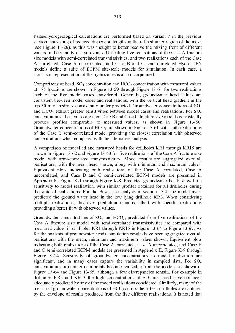
319
Palaeohydrogeological calculations are performed based on variant 7 in the previous section, consisting of reduced dispersion lengths in the refined inner region of the mesh (see Figure 13-26), as this was thought to better resolve the mixing front of different waters in the vicinity of hydrozones. Upscaling five realisations of the Case A fracture size models with semi-correlated transmissivities, and two realisations each of the Case A correlated, Case A uncorrelated, and Case B and C semi-correlated Hydro-DFN models define a suite of ECPM site-scale models for simulation. In each case, a stochastic representation of the hydrozones is also incorporated.
Comparisons of head, SO4 concentration and HCO3 concentration with measured values at 175 locations are shown in Figure 13-59 through Figure 13-61 for two realisations each of the five model cases considered. Generally, groundwater head values are consistent between model cases and realisations, with the vertical head gradient in the top 50 m of bedrock consistently under predicted. Groundwater concentrations of SO4 and HCO3 exhibit greater sensitivities between model cases and realisations. For SO4 concentrations, the semi-correlated Case B and Case C fracture size models consistently produce profiles comparable to measured values, as shown in Figure 13-60. Groundwater concentrations of HCO3 are shown in Figure 13-61 with both realisations of the Case B semi-correlated model providing the closest correlation with observed concentrations when compared with the alternative analysis.
A comparison of modelled and measured heads for drillholes KR1 through KR15 are shown in Figure 13-62 and Figure 13-63 for five realisations of the Case A fracture size model with semi-correlated transmissivities. Model results are aggregated over all realisations, with the mean head shown, along with minimum and maximum values. Equivalent plots indicating both realisations of the Case A correlated, Case A uncorrelated, and Case B and C semi-correlated ECPM models are presented in Appendix K, Figure K-1 through Figure K-8. Predicted groundwater heads show little sensitivity to model realisation, with similar profiles obtained for all drillholes during the suite of realisations. For the Base case analysis in section 13.4, the model over-predicted the ground water head in the low lying drillhole KR3. When considering multiple realisations, this over prediction remains, albeit with specific realisations providing a better fit with observed values.
Groundwater concentrations of SO4 and HCO3, predicted from five realisations of the Case A fracture size model with semi-correlated transmissivities are compared with measured values in drillholes KR1 through KR15 in Figure 13-64 to Figure 13-67. As for the analysis of groundwater heads, simulation results have been aggregated over all realisations with the mean, minimum and maximum values shown. Equivalent plots indicating both realisations of the Case A correlated, Case A uncorrelated, and Case B and C semi-correlated ECPM models are presented in Appendix K, Figure K-9 through Figure K-24. Sensitivity of groundwater concentrations to model realisation are significant, and in many cases capture the variability in sampled data. For SO4 concentrations, a number data points become realizable from the models, as shown in Figure 13-64 and Figure 13-65, although a few discrepancies remain. For example in drillholes KR2 and KR13 the high concentrations of SO4 measured have not been adequately predicted by any of the model realisations considered. Similarly, many of the measured groundwater concentrations of HCO3 across the fifteen drillholes are captured by the envelope of results produced from the five different realisations. It is noted that

320
the chemical composition of groundwaters detailed in Table 13-4 provide an upper bound of HCO3 concentration of 291 mg/L, and therefore the measured concentrations at shallow depths in drillholes KR1 and KR9 are unobtainable. It would probably be necessary to consider reactions with minerals in the near-surface to better describe heterogeneity in groundwater composition close to the surface.
In summary:
All model variants provide an acceptable match to both groundwater head and chemical measurements;
Head is relatively insensitive to stochastic variability in the hydrozones and sparsely fractured rock, varying by about ±1m for individual measurement points. Still, this envelope of simulated heads is sufficient to capture many of the measurements;
Results for simulated HCO3 and SO4 very significantly between realisations of the hydrozones and sparsely fracture rock, again capturing the measured values with the envelope of simulations even with only 5 realisations. Hence, specific measurements may be the result of local hydraulic conditions resulting from spatial variability;
Simulated hydrochemical results are more sensitive to the fracture intensity-size model than the transmissivity-size model for the model variants considered. Cases B and C giving slightly better results for HCO3 and SO4 than Case A, which corresponds with these variants giving slightly tighter overall hydraulic properties in the upper bedrock;
There is higher observed variability in HCO3 within the uppermost bedrock than reproduced in the stochastic simulation suggesting this results from variability in the effects of chemical processes in the near-surface.
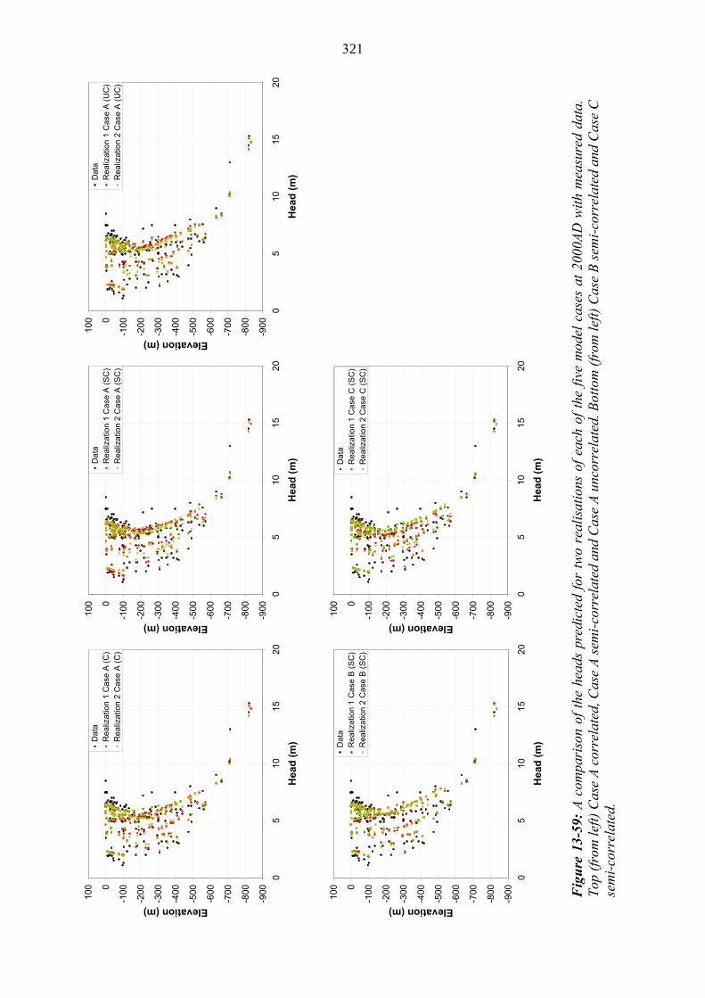
321
-900
-800
-700
-600
-500
-400
-300
-200
-1000
100
05
1015
20
Hea
d (
m)
Elevation (m)D
ata
Rea
lizat
ion
1 C
ase
A (
C)
Rea
lizat
ion
2 C
ase
A (
C)
-900
-800
-700
-600
-500
-400
-300
-200
-1000
100
05
1015
20
Hea
d (
m)
Elevation (m)
Da
taR
ea
liza
tion
1 C
ase
A (
SC
)R
ea
liza
tion
2 C
ase
A (
SC
)
-900
-800
-700
-600
-500
-400
-300
-200
-1000
100
05
1015
20
Hea
d (
m)
Elevation (m)
Da
taR
ea
liza
tion
1 C
ase
A (
UC
)R
ea
liza
tion
2 C
ase
A (
UC
)
-900
-800
-700
-600
-500
-400
-300
-200
-1000
100
05
1015
20
Hea
d (
m)
Elevation (m)
Dat
aR
ealiz
atio
n 1
Cas
e B
(S
C)
Rea
lizat
ion
2 C
ase
B (
SC
)
-900
-800
-700
-600
-500
-400
-300
-200
-1000
100
05
1015
20
Hea
d (
m)
Elevation (m)
Dat
aR
ea
liza
tion
1 C
ase
C (
SC
)R
ea
liza
tion
2 C
ase
C (
SC
)
Fig
ure
13-
59:
A c
ompa
riso
n of
the
hea
ds p
redi
cted
for
tw
o re
alis
atio
ns o
f ea
ch o
f th
e fiv
e m
odel
cas
es a
t 20
00A
D w
ith m
easu
red
data
. T
op (
from
left)
Cas
e A
cor
rela
ted,
Cas
e A
sem
i-co
rrel
ated
and
Cas
e A
unc
orre
late
d. B
otto
m (
from
left
) C
ase
B s
emi-
corr
elat
ed a
nd C
ase
C
sem
i-co
rrel
ated
.
321

322
-90
0
-80
0
-70
0
-60
0
-50
0
-40
0
-30
0
-20
0
-10
00
100
010
020
03
004
005
0060
0
SO
4 (
mg
/L)
Elevation (m)
Dat
aR
ealiz
atio
n 1
Cas
e A
(C
)R
ealiz
atio
n 2
Cas
e A
(C
)-9
00
-800
-700
-600
-500
-400
-300
-200
-1000
100
010
020
030
040
050
060
0
SO
4 (
mg
/L)
Elevation (m)
Da
taR
eal
iza
tion
1 C
ase
A (
SC
)R
eal
iza
tion
2 C
ase
A (
SC
)-9
00
-800
-700
-600
-500
-400
-300
-200
-1000
100
010
020
030
040
050
060
0
SO
4 (m
g/L
)
Elevation (m)
Data
Re
aliz
atio
n 1
Ca
se A
(U
C)
Re
aliz
atio
n 2
Ca
se A
(U
C)
-90
0
-80
0
-70
0
-60
0
-50
0
-40
0
-30
0
-20
0
-10
00
100
010
020
03
004
005
0060
0
SO
4 (
mg
/L)
Elevation (m)
Da
taR
eal
izat
ion
1 C
ase
B (
SC
)R
eal
izat
ion
2 C
ase
B (
SC
)-9
00
-80
0
-70
0
-60
0
-50
0
-40
0
-30
0
-20
0
-10
00
100
01
002
0030
04
0050
06
00
SO
4 (
mg
/L)
Elevation (m)
Da
taR
ea
lizat
ion
1 C
ase
C (
SC
)R
ea
lizat
ion
2 C
ase
C (
SC
)
Fig
ure
13-
60:
A c
ompa
riso
n of
the
SO
4 co
ncen
trat
ions
pre
dict
ed f
or t
wo
real
isat
ions
of
each
of
the
five
mod
el c
ases
at
2000
AD
with
m
easu
red
data
. T
op (
from
lef
t) C
ase
A c
orre
late
d, C
ase
A s
emi-
corr
elat
ed a
nd C
ase
A u
ncor
rela
ted.
Bot
tom
(fr
om l
eft)
Cas
e B
sem
i-co
rrel
ated
and
Cas
e C
sem
i-co
rrel
ated
.
322
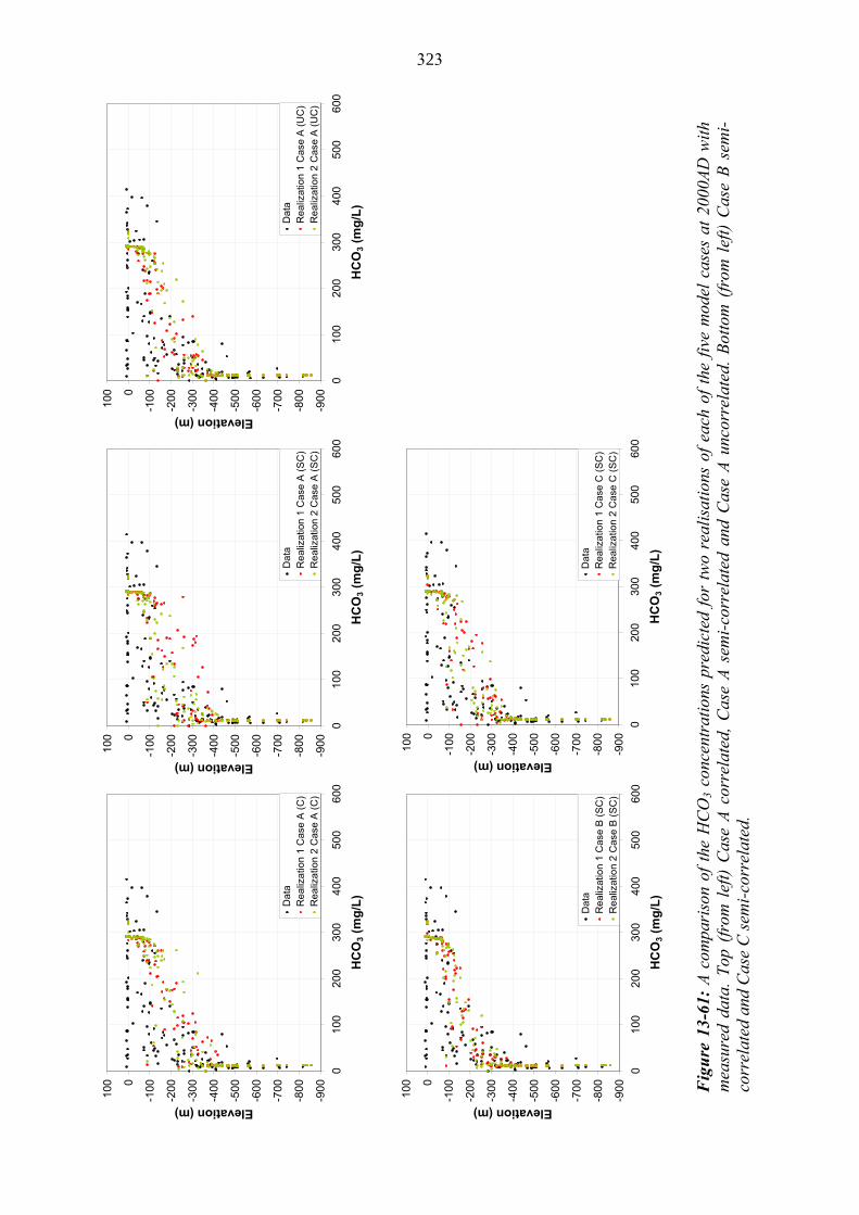
323
-900
-800
-700
-600
-500
-400
-300
-200
-1000
100
010
020
030
040
050
060
0
HC
O3 (
mg
/L)
Elevation (m)
Da
taR
eal
iza
tion
1 C
ase
A (
C)
Re
aliz
atio
n 2
Cas
e A
(C
)-9
00
-800
-700
-600
-500
-400
-300
-200
-1000
100
010
020
030
040
050
060
0
HC
O3 (
mg
/L)
Elevation (m)
Da
taR
eal
iza
tion
1 C
ase
A (
SC
)R
eal
iza
tion
2 C
ase
A (
SC
)-9
00
-800
-700
-600
-500
-400
-300
-200
-1000
100
010
020
030
040
050
060
0
HC
O3 (
mg
/L)
Elevation (m)
Da
taR
eal
izat
ion
1 C
ase
A (
UC
)R
eal
izat
ion
2 C
ase
A (
UC
)
-900
-800
-700
-600
-500
-400
-300
-200
-1000
100
010
020
030
040
050
060
0
HC
O3 (
mg
/L)
Elevation (m)
Da
taR
eal
izat
ion
1 C
ase
B (
SC
)R
eal
izat
ion
2 C
ase
B (
SC
)-9
00
-800
-700
-600
-500
-400
-300
-200
-1000
100
010
020
030
040
050
060
0
HC
O3 (
mg
/L)
Elevation (m)
Data
Re
aliz
atio
n 1
Ca
se C
(S
C)
Re
aliz
atio
n 2
Ca
se C
(S
C)
Fig
ure
13-
61:
A c
ompa
riso
n of
the
HC
O3
conc
entr
atio
ns p
redi
cted
for
tw
o re
alis
atio
ns o
f ea
ch o
f th
e fiv
e m
odel
cas
es a
t 20
00A
D w
ith
mea
sure
d da
ta.
Top
(fr
om l
eft)
Cas
e A
cor
rela
ted,
Cas
e A
sem
i-co
rrel
ated
and
Cas
e A
unc
orre
late
d. B
otto
m (
from
lef
t) C
ase
B s
emi-
corr
elat
ed a
nd C
ase
C s
emi-
corr
elat
ed.
323
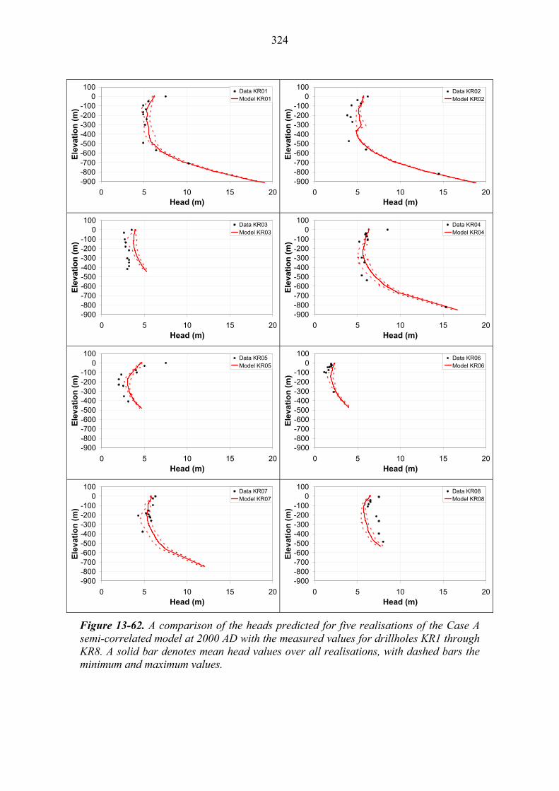
324
-900-800-700-600-500-400-300-200-100
0100
0 5 10 15 20Head (m)
Ele
vati
on
(m
)
Data KR01Model KR01
-900-800-700-600-500-400-300-200-100
0100
0 5 10 15 20Head (m)
Ele
vati
on
(m
)
Data KR02Model KR02
-900-800-700-600-500-400-300-200-100
0100
0 5 10 15 20Head (m)
Ele
vati
on
(m
)
Data KR03Model KR03
-900-800-700-600-500-400-300-200-100
0100
0 5 10 15 20Head (m)
Ele
vati
on
(m
)
Data KR04Model KR04
-900-800-700-600-500-400-300-200-100
0100
0 5 10 15 20Head (m)
Ele
vati
on
(m
)
Data KR05Model KR05
-900-800-700-600-500-400-300-200-100
0100
0 5 10 15 20Head (m)
Ele
vati
on
(m
)
Data KR06Model KR06
-900-800-700-600-500-400-300-200-100
0100
0 5 10 15 20Head (m)
Ele
vati
on
(m
)
Data KR07Model KR07
-900-800-700-600-500-400-300-200-100
0100
0 5 10 15 20Head (m)
Ele
vati
on
(m
)
Data KR08Model KR08
Figure 13-62. A comparison of the heads predicted for five realisations of the Case A semi-correlated model at 2000 AD with the measured values for drillholes KR1 through KR8. A solid bar denotes mean head values over all realisations, with dashed bars the minimum and maximum values.
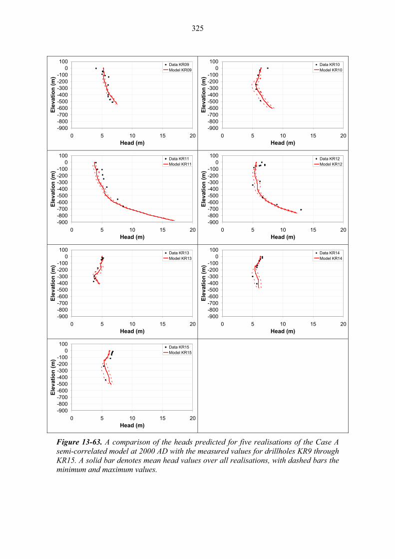
325
-900-800-700-600-500-400-300-200-100
0100
0 5 10 15 20Head (m)
Ele
vati
on
(m
)
Data KR09Model KR09
-900-800-700-600-500-400-300-200-100
0100
0 5 10 15 20Head (m)
Ele
vati
on
(m
)
Data KR10Model KR10
-900-800-700-600-500-400-300-200-100
0100
0 5 10 15 20Head (m)
Ele
vati
on
(m
)
Data KR11Model KR11
-900-800-700-600-500-400-300-200-100
0100
0 5 10 15 20Head (m)
Ele
vati
on
(m
)
Data KR12Model KR12
-900-800-700-600-500-400-300-200-100
0100
0 5 10 15 20Head (m)
Ele
vati
on
(m
)
Data KR13Model KR13
-900-800-700-600-500-400-300-200-100
0100
0 5 10 15 20Head (m)
Ele
vati
on
(m
)
Data KR14Model KR14
-900-800-700-600-500-400-300-200-100
0100
0 5 10 15 20Head (m)
Ele
vati
on
(m
)
Data KR15Model KR15
Figure 13-63. A comparison of the heads predicted for five realisations of the Case A semi-correlated model at 2000 AD with the measured values for drillholes KR9 through KR15. A solid bar denotes mean head values over all realisations, with dashed bars the minimum and maximum values.

326
-900-800-700-600-500-400-300-200-100
0100
0 100 200 300 400 500 600SO4 (mg/L)
Ele
vati
on
(m
)
Data KR01Model KR01
-900-800-700-600-500-400-300-200-100
0100
0 100 200 300 400 500 600SO4 (mg/L)
Ele
vati
on
(m
)
Data KR02Model KR02
-900-800-700-600-500-400-300-200-100
0100
0 100 200 300 400 500 600SO4 (mg/L)
Ele
vati
on
(m
)
Data KR03Model KR03
-900-800-700-600-500-400-300-200-100
0100
0 100 200 300 400 500 600SO4 (mg/L)
Ele
vati
on
(m
)
Data KR04Model KR04
-900-800-700-600-500-400-300-200-100
0100
0 100 200 300 400 500 600SO4 (mg/L)
Ele
vati
on
(m
)
Data KR05Model KR05
-900-800-700-600-500-400-300-200-100
0100
0 100 200 300 400 500 600SO4 (mg/L)
Ele
vati
on
(m
)
Data KR06Model KR06
-900-800-700-600-500-400-300-200-100
0100
0 100 200 300 400 500 600SO4 (mg/L)
Ele
vati
on
(m
)
Data KR07Model KR07
-900-800-700-600-500-400-300-200-100
0100
0 100 200 300 400 500 600SO4 (mg/L)
Ele
vati
on
(m
)
Data KR08Model KR08
Figure 13-64. A comparison of the SO4 concentrations predicted for five realisations of the Case A semi-correlated model at 2000 AD with the measured values for drillholes KR1 through KR8. A solid bar denotes mean head values over all realisations, with dashed bars the minimum and maximum values.
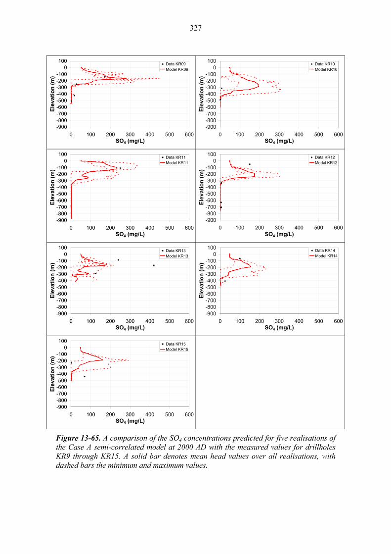
327
-900-800-700-600-500-400-300-200-100
0100
0 100 200 300 400 500 600SO4 (mg/L)
Ele
vati
on
(m
)
Data KR09Model KR09
-900-800-700-600-500-400-300-200-100
0100
0 100 200 300 400 500 600SO4 (mg/L)
Ele
vati
on
(m
)
Data KR10Model KR10
-900-800-700-600-500-400-300-200-100
0100
0 100 200 300 400 500 600SO4 (mg/L)
Ele
vati
on
(m
)
Data KR11Model KR11
-900-800-700-600-500-400-300-200-100
0100
0 100 200 300 400 500 600SO4 (mg/L)
Ele
vati
on
(m
)
Data KR12Model KR12
-900-800-700-600-500-400-300-200-100
0100
0 100 200 300 400 500 600SO4 (mg/L)
Ele
vati
on
(m
)
Data KR13Model KR13
-900-800-700-600-500-400-300-200-100
0100
0 100 200 300 400 500 600SO4 (mg/L)
Ele
vati
on
(m
)
Data KR14Model KR14
-900-800-700-600-500-400-300-200-100
0100
0 100 200 300 400 500 600SO4 (mg/L)
Ele
vati
on
(m
)
Data KR15Model KR15
Figure 13-65. A comparison of the SO4 concentrations predicted for five realisations of the Case A semi-correlated model at 2000 AD with the measured values for drillholes KR9 through KR15. A solid bar denotes mean head values over all realisations, with dashed bars the minimum and maximum values.
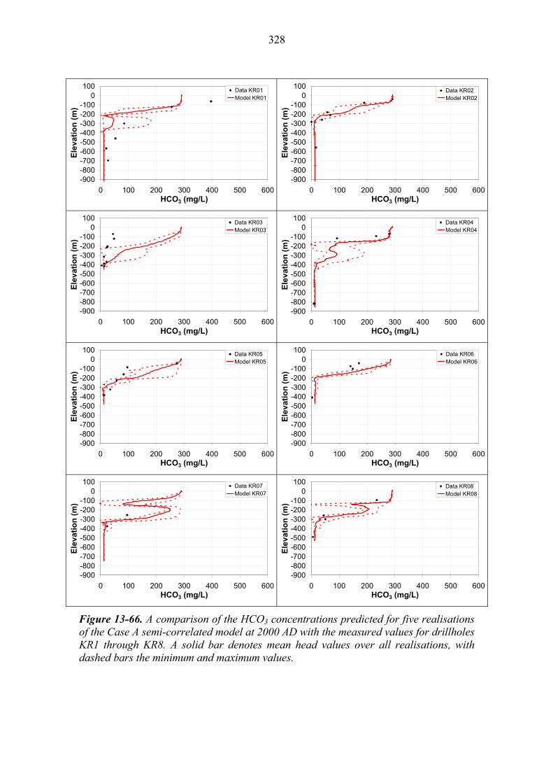
328
-900-800-700-600-500-400-300-200-100
0100
0 100 200 300 400 500 600HCO3 (mg/L)
Ele
vati
on
(m
)
Data KR01Model KR01
-900-800-700-600-500-400-300-200-100
0100
0 100 200 300 400 500 600HCO3 (mg/L)
Ele
vati
on
(m
)
Data KR02Model KR02
-900-800-700-600-500-400-300-200-100
0100
0 100 200 300 400 500 600HCO3 (mg/L)
Ele
vati
on
(m
)
Data KR03Model KR03
-900-800-700-600-500-400-300-200-100
0100
0 100 200 300 400 500 600HCO3 (mg/L)
Ele
vati
on
(m
)
Data KR04Model KR04
-900-800-700-600-500-400-300-200-100
0100
0 100 200 300 400 500 600HCO3 (mg/L)
Ele
vati
on
(m
)
Data KR05Model KR05
-900-800-700-600-500-400-300-200-100
0100
0 100 200 300 400 500 600HCO3 (mg/L)
Ele
vati
on
(m
)
Data KR06Model KR06
-900-800-700-600-500-400-300-200-100
0100
0 100 200 300 400 500 600HCO3 (mg/L)
Ele
vati
on
(m
)
Data KR07Model KR07
-900-800-700-600-500-400-300-200-100
0100
0 100 200 300 400 500 600HCO3 (mg/L)
Ele
vati
on
(m
)
Data KR08Model KR08
Figure 13-66. A comparison of the HCO3 concentrations predicted for five realisations of the Case A semi-correlated model at 2000 AD with the measured values for drillholes KR1 through KR8. A solid bar denotes mean head values over all realisations, with dashed bars the minimum and maximum values.

329
-900-800-700-600-500-400-300-200-100
0100
0 100 200 300 400 500 600HCO3 (mg/L)
Ele
vati
on
(m
)
Data KR09Model KR09
-900-800-700-600-500-400-300-200-100
0100
0 100 200 300 400 500 600HCO3 (mg/L)
Ele
vati
on
(m
)
Data KR10Model KR10
-900-800-700-600-500-400-300-200-100
0100
0 100 200 300 400 500 600HCO3 (mg/L)
Ele
vati
on
(m
)
Data KR11Model KR11
-900-800-700-600-500-400-300-200-100
0100
0 100 200 300 400 500 600HCO3 (mg/L)
Ele
vati
on
(m
)
Data KR12Model KR12
-900-800-700-600-500-400-300-200-100
0100
0 100 200 300 400 500 600HCO3 (mg/L)
Ele
vati
on
(m
)
Data KR13Model KR13
-900-800-700-600-500-400-300-200-100
0100
0 100 200 300 400 500 600HCO3 (mg/L)
Ele
vati
on
(m
)
Data KR14Model KR14
-900-800-700-600-500-400-300-200-100
0100
0 100 200 300 400 500 600HCO3 (mg/L)
Ele
vati
on
(m
)
Data KR15Model KR15
Figure 13-67. A comparison of the HCO3 concentrations predicted for five realisations of the Case A semi-correlated model at 2000 AD with the measured values for drillholes KR9 through KR15. A solid bar denotes mean head values over all realisations, with dashed bars the minimum and maximum values.

330
13.6 Palaeohydrogeological analysis – transmissivity calibrations
Site-scale confirmatory analysis through prediction of baseline heads and drawdown for four pumping tests were detailed in Sections 13.1 and 13.2, respectively. Calibrations suggested modifications to transmissivities of both the hydrozones and stochastically generated background fractures. The effects on groundwater evolution and palaeohydrogeology predictions when incorporating the calibrated hydrozone transmissivities described in Section 13.2 are examined in this section. Palaeohydrogeological variations caused by adjustment of background fracture transmissivities are not considered.
A single realisation of the Case A fracture size model with semi-correlated transmissivities is considered, with deterministically specified hydrozones incorporated. Modifications to hydrozones determined through the calibration process are detailed in Section 13.2. In general, hydrozones become more transmissive, especially at shallow depths, for HZ19A, HZ19B, HZ19C, HZ20A and HZ20B. Simulations are based on variant 7 of the sensitivity study, with reduced dispersion lengths specified on the region of refined mesh at the centre of the island (Figure 13-26).
Figure 13-68 shows a comparison of groundwater heads predicted from simulations using both the original and calibrated hydrozone description with measured values at 175 locations. Figure 13-69 and Figure 13-70 make the equivalent comparison for groundwater concentrations of SO4 and HCO3. The differences are slight relative to the sensitivities to uncertainties explored in Sections 13.5. Hence, the changes to specific hydrozone properties suggested by calibration on the pumping tests in Section 13.2 are still consistent with the palaeohydrogeological confirmatory tests. In terms of an overall calibration then, the changes suggested in Section 13.2 should be included in the hydrogeological description.
-900
-800
-700
-600
-500
-400
-300
-200
-100
0
100
0 2 4 6 8 10 12 14 16 18 20
Head (m)
Ele
vati
on
(m
)
DataOriginal HydrozonesCalibrated Hydrozones
Figure 13-68. A comparison of the heads predicted for a single realisation of Case A semi-correlated fracture network for both the original and calibrated hydrozone description with measured values.

331
-900
-800
-700
-600
-500
-400
-300
-200
-100
0
100
0 100 200 300 400 500 600
SO4 (mg/L)
Ele
vati
on
(m
)
DataOriginal HydrozonesCalibrated Hydrozones
Figure 13-69. A comparison of the SO4 concentrations predicted for a single realisation of the Case A semi-correlated fracture network for both the original and calibrated hydrozone description with measured values.
-900
-800
-700
-600
-500
-400
-300
-200
-100
0
100
0 100 200 300 400 500 600
HCO3 (mg/L)
Ele
vati
on
(m
)
DataOriginal HydrozonesCalibrated Hydrozones
Figure 13-70. A comparison of the HCO3 concentrations predicted for a single realisation of the Case A semi-correlated fracture network for both the original and calibrated hydrozone description with measured values.

332
333
14 SUMMARY AND CONCLUSIONS
14.1 Summary for Phase I
Phase I of the Hydro-DFN update has the objective of updating the Olkiluoto Hydro-DFN model based on the updated frameworks of the geological modelling /Aaltonen et al. 2010/, the Geo-DFN modelling /Fox et al. 2011/ and the hydro-structural model /Vaittinen et al. 2011/ together with the inclusion of additional drillhole data. The results are the definition of appropriate hydraulic domains and the parameterisation of the Hydro-DFN model within each, and associated alternative model cases to address some of the important conceptual uncertainties, namely appropriate intensity-size-transmissivity models for potential flowing fractures.
14.1.1 Data analysis
Analysis of the primary fracture data involves the interpretation of Posiva’s fracture database and Posiva Flow Log (PFL) data from 80 surface drilled drillholes and 15 pilot holes, as well as Hydraulic Test Unit (HTU) data. A consistency with the Geo-DFN modelling of /Fox et al. 2011/ is ensured by sharing a common database (as of 24th June 2010). For the specific purposes of the Hydro-DFN modelling, the database complemented with data from PFL measurements was used to get an orientation estimate for the observed flowing fractures to ensure the maximum number of PFL measurements are accounted for in the analysis. By applying these measures were able to increase the portion of PFL measurements used in the analysis from 90.6 % to 98.5 % without introducing any discernible bias, and thereby utilise virtually the full distribution of specific capacities and honour the measured flowing fracture intensity.
The definition of suitable hydraulic domains starts from the geological framework of nine tectonic units specified in /Aaltonen et al. 2010/. To obtain statistical significance in the analysis of the PFL data within a sub-domain it is preferable to limit the number of hydraulic domains to as few as obscuring genuine trends such as changes relative intensity or rotation of mean poles.. Based on comparing characteristics in the orientations and intensities of both all fractures and PFL fractures, then the sub-division of the Hydro-DFN model limits the geological framework of nine tectonic units to the following four hydraulic domains:
1. NTU + SDZ becoming NHU;
2. CTU1 + CTU2 + FSZ becoming CHUW;
3. CTU3 + D4 becoming CHUE;
4. STU + LSZ becoming SHU.
Of these four, NHU and CHUW have good data coverage; CHUE is more limited, but has some data covering repository depth; data in SHU is also limited and there is none below -400 m.
As with the 2008 Hydro-DFN /Hartley et al. 2009/, a very significant reduction in both the intensity of PFL fractures and effective hydraulic conductivity with depth is apparent in the data. In the 2008 Hydro-DFN /Hartley et al. 2009/, this depth trend was

334
represented by division in to four fixed depth zones with boundaries at -50 m, -150 m and -400 m. For the update it is noted that although this broad description is still valid, there are significant lateral variations in the intensities of PFL fractures. Hence, the methodology for defining depth zones is refined to use a division of each individual drillhole into four depth zones according to hydraulic and hydrochemical characteristics of the bedrock. The hydraulic characteristic used is the intensity of PFL fractures outside of hydrozones as measured in 50 m intervals in elevation. The boundaries between the depth zones are then obtained over the site-scale by interpolating between the depth zones interpreted in each of the drillholes, which results in three surfaces delimiting both vertical and lateral variations in hydraulic fracture characteristics (hydrochemical data is also used as confirmatory information, but there are relatively few samples compared to PFL intensities).
The basis for analysis of fracture orientations were the three sets (EW, NS and SH) as used previously in the 2008 Hydro-DFN. Consistent with the updated Geo-DFN of /Fox et al. 2011/, the sub-vertical sets are parameterised by fitting a Univariate Fisher distribution, while a Bivariate Bingham distribution is fitted to the sub-horizontal set to better capture the typically elongated distribution of fracture orientations within this set. For the Hydro-DFN, orientations parameters are obtained by fitting the observed poles for PFL fractures, so that generated Hydro-DFN models are statistically similar to the subset of PFL fractures in terms of orientation. Orientation parameters are interpreted for the PFL fractures by hydraulic domain. The updated Geo-DFN interprets 13 fracture sets in total, with some specific sets for particular fracture domains, and some common across domains. However, the mean poles of these sets are generally with 10º of those for the corresponding sets interpret in the Hydro-DFN.
An estimate for the intensity of Open fractures is made based on the Geo-DFN analysis of the geological indicators for All fractures augmented by consideration of any correlation with PFL fractures. In the 2008 Hydro-DFN, the frequency of Open fractures was estimated as the upper limit of the intensity of potential flowing fractures based on the geological classification to Tight, Open and Filled fractures. The updated definition of Open fractures is based on the Geo-DFN definition for Open, Flowing and closed fractures with some modifications for the Hydro-DFN application. Modifications were necessary to account for data gaps in the Posiva fracture database. Definitions of the Geo-DFN Open and Closed fractures for All fractures and PFL fractures from KR1 through KR38 were used to estimate a suitable ratio of Open fractures to all fractures likely to capture all PFL fractures, which can then be applied across all drillholes and at each depth zone. It should be noted that this method only provides an estimate of Open fracture intensity; it does not predict if an individual fracture is open based on the geological indicators. This estimate of Open fracture intensity is only used in one of three intensity-size models, Case A, considered in the Hydro-DFN modelling. The analysis of Open fractures is not used for any other purpose.
Summary tables are produced of Terzaghi corrected fracture intensities calculated for All fractures, Open fractures and PFL fractures by hydraulic domain and depth zone. Similar statistics for the effective hydraulic conductivity, sum of transmissivities over drillhole length, and maximum transmissivity are also tabulated. This approach has been applied previously for Forsmark /Follin et al. 2007/ and Laxemar /Rhén et al. 2008/.
335
Appropriate models for the distribution of transmissivity with hydrozones are considered using the updated hydrogeological structural model /Vaittinen et al. 2011/. The measured transmissivities within each hydrozones show typically four orders of magnitude variability, making the interpretation of appropriate parameters over these structures uncertain. Within each hydrozone, there is a gradual reduction in the maximum measured transmissivity with depth and in the geometric mean within a depth zone. Hence, for the purposes of the Hydro-DFN modelling performed here, a gradual depth trend in mean transmissivity has been interpreted, but with significant spatial variability. This formulation of the hydrozone transmissivity is implemented as a three-dimensional hydrozone model with each hydrozone represented as a triangulated surface with triangles of side 200m to capture the non-planar geometry of the structure and variations in transmissivity across the zone, 200m being an approximate spacing of measurement points in drillholes. The transmissivity of the triangles is assigned based on either the interpreted deterministic gradual depth trend or as stochastic heterogeneous realisations based on sampling the variability, but in each case conditioning the local transmissivity to the measured values at the drillhole intercepts (i.e. replacing the sampled transmissivity in the intercepted triangle with the measured value).
Comparisons are made of intensities of all and PFL fractures seen in surface drilled drillholes and ONKALO pilot holes. The intensities of all fractures are broadly compatible, about 45% higher for the pilot holes. This difference may reflect spatial variability, or the fact that the pilot holes are all above –420m while the some KR holes go deeper into slightly less fractured rock, or possibly be due to different conditions for geological fracture characterisation in the ONKALO, for example. The intensities of PFL fractures are higher in the pilot holes. However, the main reason for this seems to be the lower detection limit on transmissivity prevalent in the pilot holes resulting from a much higher drawdown used in these tests relative to the KR drillholes. If a filter on interpreted transmissivity of 1-2 10-9 m2/s is applied, then PFL intensities between the surface drilled and pilot holes are consistent. Still, it has to be recognised that there may be differences in test conditions resulting from the pilot holes being horizontal and less likely to intersect the dominant sub-horizontal set, as well as some effects from disturbances caused by the excavation such as some dewatering or grout injection near the ONKALO. The significantly different detection limit between the surface drilled and pilot holes raises issues of whether the two set of data yield consistent statistics for fracture intensity at repository depth, and wider conceptual issues of what ranges of transmissivity need to be considered in the Hydro-DFN model, which were the subject of additional analysis in Phase III once data from additional pilot holes became available.
Comparing the 2008 Hydro-DFN and the updated Hydro-DFN analysis, the extra available data has not resulted in significant changes in understanding of the hydraulic fractures. The methodological changes introduced here, such as the use of a Bingham distribution of sub-horizontal fracture orientation and the definition of depth zones that vary laterally are not fundamental changes in thinking, rather attempts to honour more details of the available site data. Very similar depth profiles of PFL intensity are obtained now as in 2008. There is a slight increase in PFL intensity, mainly for the upper 150m of bedrock, for the update due to the steps introduced to ensure virtually all PFL measurements are assigned to a fracture and assigned an orientation. The effective
336
hydraulic conductivity of the bedrock between hydrozones is reduced relative to 2008 as a result of greater care taken in assessing the relationship between high transmissivity features and the hydrogeological structural model /Vaittinen et al. 2011/.
A comparison of transmissivities interpreted from HTU test intervals based on the double-packer constant-head method, and those derived from summing PFL transmissivities for the corresponding drillhole/HTU interval is made. A reasonable correlation, within one order of magnitude, is obtained for the majority of intervals outside hydrozones. Initial investigations into the outlier points, and intervals for which there is HTU flow, but no PFL measurements are identified, are inconclusive. In some cases PFL measurements were found relatively close to the HTU interval, which could suggest that the HTU depth measurements were not sufficiently accurate, while in other cases no PFL measurements at all could be found within 5 m of the HTU interval. Such discrepancies may result from leakage/short circuit flows around the packer system, or given the HTU tests are based on injection for 20 minutes, while the PFL tests involve pumping for several days, be an indication of finite compartments or hydraulic chokes. This needs further investigation.
Another issue that was analysed in the Hydro-DFN was the possible role of clustering with of the stochastic fractures associated with minor fracture zones. The updated Geo-DFN model /Fox et al. 2011/, identified drillhole intervals with increased fracture intensity outside of the hydrozones where fractures appear to occur in “clusters”. For consistency with the Hydro-DFN conceptual model, any PFL fractures within these clusters should also be grouped together and the transmissivity of the individual PFL fractures summed for the combined single feature. Such a treatment of the clusters has not been performed in this study because not all the required information is available to make a complete analysis. However, the interval information provided by the Geo-DFN analysis alone is sufficient to quantify by how much key results presented in this report would be changed if fracture clusters were taken into account. It is found that clusters would reduce PFL intensity by about 5 % above -400 m, but make no difference below that depth (i.e. repository depth). However, clusters would result in about 10-15 % reduction in the intensity of all fractures at most depths. It is therefore concluded that although the clusters interpreted by the Geo-DFN have clear significance for fracture occurrence, their affect on the spatial distribution of flowing fractures is relatively minor, about 5 %.
14.1.2 Hydro-DFN model calibration
The Hydro-DFN model involves a prescription for statistical distributions for orientation, intensity, size and transmissivity of the potentially flowing fractures, i.e. those containing void space within the fracture. This is a sub-set of All fractures, as Sealed fractures are excluded, and hence a sub-set of the fractures described by the Geo-DFN. PFL fractures are a sub-set of the potentially flowing fractures represented by the Hydro-DFN, being those that form part of a connected network and have a sufficient specific flow capacity to be detected by PFL hydraulic tests. It is necessary to consider all potential flowing fractures rather than just those detected by PFL tests, since the ability of a fracture to carry flow can be changed due to the effects of underground excavations creating extra connections or changing stress, or changes in boundary conditions. The flowing fractures detected by PFL tests are subject to the connectivity
337
of the network when the test was performed, and the hydraulic gradients under which the test was performed. In other words, under other conditions, the connectivity and flow may be different.
The intensity and size distribution of potential flowing fractures is uncertain and hence three quite different alternative conceptual approaches have been developed to scope the implications of necessary assumptions made about these parameters:
Case A – A model based on estimated intensity of Open fractures, using a power-law size model;
Case B – A model based on the intensity of PFL fractures, using a log-normal size model;
Case C – A model based on the intensity of all fractures, using a global power-law size model derived for the Geo-DFN, but removing parts of the fracture surface area available for flow according to some probability function that depends on fracture size (i.e. a larger proportion of fracture surface area is open in large fractures than small)
These definitions provide specifications for the intensity of potentially flowing fractures that can be obtained from the analysis of different portions of the total fracture intensity. They correspond to approximately: Case A ~31 %, Case B ~6 %, and Case C ~100 % (although in this case only a portion of the area is open to flow) of the intensity of All fractures.
Fracture size distributions for each case are determined by two constraints. The first is that the simulated intensity of connected fractures is equal to the measured intensity of PFL fractures. The second is a bounding constraint that the intensity of potential flowing fractures within any size range is less than that of interpreted by the Geo-DFN for all fractures within the same range. This is to ensure internal consistency with the Geo-DFN interpretation of intensity-size. For Case A with a power-law size model, simulations of fracture connectivity are required to ensure these constraints are met by adjusting the size power-law parameters (r0, kr). For Case B, the first constraint is met by definition providing fracture sizes are large enough that most potentially flowing fractures are connected, but not so large as to break the second constraint. Appropriate parameters for the log-normal distribution used in Case B can be estimated by analytical means, and then check by simulations of connectivity. For Case C, the intensity and power-law size model are fixed based a global size model from the Geo-DFN (r0=0.2 m, kr=2.59), and so the second constraint is met by definition. The first constraint is met by performing simulations of fracture connectivity and adjusting the proportion of fracture area that is open. As a starting point only 49 % of fracture area is assumed to be open based on the fact that the intensity of the interpreted hydrozones is only 49 % of the intensity of brittle deformation zones.
Fracture network simulations are performed in two main steps. The first step is to simulate the connectivity of the network as seen in sample drillholes to calibrate the geometrical parameters. The second step simulates the PFL test conditions modelling flows through the network to drillholes in order to calibrate the fracture transmissivities.
338
The DFN simulations of conditions around drillholes consider the following representative drillholes:
NHU KR1, KR2, KR11 and KR43;
CHUW KR8, KR24, KR38 and KR48;
CHUE KR45, KR49 and KR50;
SHU KR51, KR52 and KR53.
For each hydraulic domain and depth zone, 10-13 realisations are performed of each drillhole to provide a total of 39 or 40 realisations that are used to form ensemble statistics from the model that are compared with pooled statistics from the data for the drillholes in the corresponding sub-domains. Based on these simulations, fracture size parameters have been defined for each model case, hydraulic domain, depth zone and set. The intensity-size distributions of the connected fractures for each of the three model cases A-C show considerable consistency resulting from the geometrical constraints. There are differences though, Case A tends to have the highest intensity of small fractures (c. 1m), Case C tends to have the highest of large fractures (c. 500 m), and Case B has the highest intensity of medium size fractures (c. 30 m). In each case fractures larger than 20 m side (10.56 m radius) are tessellated into sub-fractures of side c. 20 m.
Simulations of flow to drillholes follow a similar approach to the connectivity analysis using representative drillholes. Three alternative fracture size-transmissivity relationships are considered for the Case A intensity size model based on a direct correlation, no correlation, and a correlation with variability superimposed (semi-correlated). Case B and Case C only consider the semi-correlated model as it is considered more realistic. Hence, five model cases are each calibrated to the same PFL flow measurements for each hydraulic domain and depth zone. The simulation results and measurements are compared in terms of statistical comparisons of the following three main measures of how well the model simulates the flow data:
1. A histogram of the distribution of specific capacities, Q/s, is compared with a bin size of half an order of magnitude (the shapes of distribution are compared by eye and by calculating the correlation coefficients).
2. The total flow to each depth zone of a drillhole, sum of Q/s.
3. The number of PFL measurements associated with each fracture set, and the distribution of Q/s for each set. This distribution is quantified in terms of the mean, plus/minus one standard deviation, minimum and maximum of log(Q/s).
All the above use Terzaghi weighting to compensate for bias they may otherwise result form the relative orientation of drillholes and fractures. The first measure checks the distribution of different specific capacities is reproduced. It can be compared visually or by calculating the correlation coefficient between the modelled and measured histograms. The second measure ensures the total flow through the each hydraulic domain and depth zone is reproduced in the model. The third measure checks the
339
correct intensity of flowing fractures is reproduced for each set and that any differences in the distributions of specific capacity between the sets are captured in the model.
The results of this process are a complete parameterisation of the Hydro-DFN model (see Table 5-8, Table 5-9,Table 5-10, for hydraulic domain NHU) for five alternative model cases , four hydraulic domains, four depth zones, and three sets. There is little or no data for Depth Zone 4 in CHUE and SHU and so it is recommended that these sub-domains be parameterised by analogy to Depth Zone 4 in CHUW. Properties such as PFL intensity and effective hydraulic conductivity can be compared between the hydraulic domains for Depth Zones 1-3 in Table 4-5 through Table 4-7. These suggest similar trends and absolute values between the hydraulic domains, and hence the analogy seems appropriate.
14.1.3 Hydraulic block properties
A Hydro-DFN description of bedrock fracture properties can be converted to effective hydraulic conductivities and kinematic porosities on a defined scale for use in Equivalent Continuous Porous Medium (ECPM) models. This involves a process of upscaling and the methodology used here is based on flow and connectivity calculations for a defined block volume using a discrete fracture network flow model. A 50 m block scale has been used as typical of the resolution of grids used in site-scale ECPM models, although finer grids may be used around the ONKALO and repository. Effective block properties are calculated for 9×9×9 (729) 50 m adjacent blocks within an overall cube with size (500 m)3 to provide statistics of the properties. For each block, simulations of flow are calculated for a volume of 150m side, but the flow-rate is only analysed through the central 50 m block to limit the contribution of fractures that are only connected locally, but not to the wider network.
The derived effective block properties provide a means to compare the five alternative Hydro-DFN model cases derived and to compare with the 2008 Hydro-DFN model. It should be noted that the model for transport aperture used here is based on 10 times the hydraulic aperture (from the cubic relationship to transmissivity), rather than the 4 times used in the 2008 Hydro-DFN, and hence kinematic porosity would be expected to increase by a factor 2.5.
For all hydraulic domains and model cases, the geometric mean of the effective hydraulic conductivity (as defined in Equation 6-1) of 50 m blocks decreases by approximately one order of magnitude per depth zone and by about half order of magnitude for kinematic porosity. This depth trend is greater than the variability between the five model cases used to explore uncertainties in Hydro-DFN and generally greater than the variability in effective hydraulic conductivity between 50 m blocks. The variation between the five different Hydro-DFN model cases is about half an order of magnitude. There is no coherent trend, although a correlated transmissivity model often seems to bias toward higher values, presumably because there is a higher probability of generating extensive high transmissivity fractures. Case C gives the lowest hydraulic conductivity. The hydraulic conductivities seem to be slightly lower in hydraulic domains CHUE and SHU than NHU and CHUW. Although this may just be a result of there being less variability in the data for CHUE and SHU because there are fewer drillholes in these domains, and hence there is less chance of measuring extreme values that can sometimes skew statistics such as total flow per unit length. The hydraulic
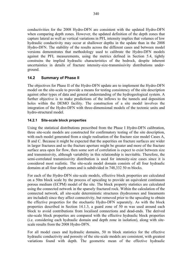
340
conductivities for the 2008 Hydro-DFN are consistent with the updated Hydro-DFN when comparing depth zones. However, the updated definition of the depth zones that capture lateral as well as vertical variations in PFL intensity implies that volumes of low hydraulic conductivity may occur at shallower depths in the update than in the 2008 Hydro-DFN. The stability of the results across the different cases and between model versions demonstrates that methodology used to calibrate the Hydro-DFN models against the PFL measurements, using the metrics defined in Section 5.4, tightly constrains the implied hydraulic characteristics of the bedrock, despite inherent uncertainties in details of fracture intensity-size-transmissivity distributions under-ground.
14.2 Summary of Phase II
The objectives for Phase II of the Hydro-DFN update are to implement the Hydro-DFN model on the site-scale to provide a means for testing consistency of the site description against other types of data and general understanding of the hydrogeological system. A further objective is to make predictions of the inflows to the tunnels and deposition holes within the DEMO facility. The construction of a site model involves the integration of the Hydro-DFN with three-dimensional models of the tectonic units and hydro-structural model.
14.2.1 Site-scale block properties
Using the statistical distributions prescribed from the Phase I Hydro-DFN calibration, three site-scale models are constructed for confirmatory testing of the site description, with each model generated from a single realisation of the fracture size model Cases A, B and C. Because it might be expected that the asperities on fracture surfaces are wider in larger fractures and so the fracture aperture might be greater and more of the fracture surface area open for flow, then some sort of correlation is expect to exist between size and transmissivity, although variability in this relationship is inevitable. Therefore, the semi-correlated transmissivity distribution is used for intensity-size cases since it is considered most realistic. The site-scale model domain consists of all four hydraulic domains at all four depth zones and is subdivided in 748,332 50 m blocks.
For each of the Hydro-DFN site-scale models, effective block properties are calculated on a 50m block scale by the process of upscaling to provide an equivalent continuum porous medium (ECPM) model of the site. The block property statistics are calculated using the connected network in the sparsely fractured rock. Within the calculation of the connected network, all site-scale deterministic structures (hydrozones and lineaments are included) since they affect connectivity, but removed prior to the upscaling to obtain the effective properties for the stochastic Hydro-DFN separately. As with the block properties described in Section 14.1.3, a guard zone of 50 m was used around each block to avoid contributions from localised connections and dead-ends. The derived site-scale block properties are compared with the effective hydraulic block properties (i.e. considering each hydraulic domain and depth zone in isolation), along with site-scale results from the 2008 Hydro-DFN.
For all model cases and hydraulic domains, 50 m block statistics for the effective hydraulic conductivity and porosity of the site-scale models are consistent, with greatest variations found with depth. The geometric mean of the effective hydraulic
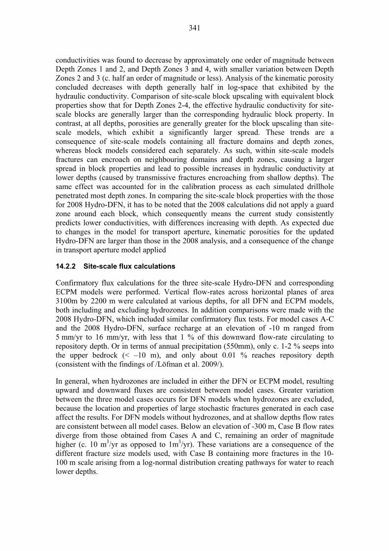
341
conductivities was found to decrease by approximately one order of magnitude between Depth Zones 1 and 2, and Depth Zones 3 and 4, with smaller variation between Depth Zones 2 and 3 (c. half an order of magnitude or less). Analysis of the kinematic porosity concluded decreases with depth generally half in log-space that exhibited by the hydraulic conductivity. Comparison of site-scale block upscaling with equivalent block properties show that for Depth Zones 2-4, the effective hydraulic conductivity for site-scale blocks are generally larger than the corresponding hydraulic block property. In contrast, at all depths, porosities are generally greater for the block upscaling than site-scale models, which exhibit a significantly larger spread. These trends are a consequence of site-scale models containing all fracture domains and depth zones, whereas block models considered each separately. As such, within site-scale models fractures can encroach on neighbouring domains and depth zones, causing a larger spread in block properties and lead to possible increases in hydraulic conductivity at lower depths (caused by transmissive fractures encroaching from shallow depths). The same effect was accounted for in the calibration process as each simulated drillhole penetrated most depth zones. In comparing the site-scale block properties with the those for 2008 Hydro-DFN, it has to be noted that the 2008 calculations did not apply a guard zone around each block, which consequently means the current study consistently predicts lower conductivities, with differences increasing with depth. As expected due to changes in the model for transport aperture, kinematic porosities for the updated Hydro-DFN are larger than those in the 2008 analysis, and a consequence of the change in transport aperture model applied
14.2.2 Site-scale flux calculations
Confirmatory flux calculations for the three site-scale Hydro-DFN and corresponding ECPM models were performed. Vertical flow-rates across horizontal planes of area 3100m by 2200 m were calculated at various depths, for all DFN and ECPM models, both including and excluding hydrozones. In addition comparisons were made with the 2008 Hydro-DFN, which included similar confirmatory flux tests. For model cases A-C and the 2008 Hydro-DFN, surface recharge at an elevation of -10 m ranged from 5 mm/yr to 16 mm/yr, with less that 1 % of this downward flow-rate circulating to repository depth. Or in terms of annual precipitation (550mm), only c. 1-2 % seeps into the upper bedrock (< –10 m), and only about 0.01 % reaches repository depth (consistent with the findings of /Löfman et al. 2009/).
In general, when hydrozones are included in either the DFN or ECPM model, resulting upward and downward fluxes are consistent between model cases. Greater variation between the three model cases occurs for DFN models when hydrozones are excluded, because the location and properties of large stochastic fractures generated in each case affect the results. For DFN models without hydrozones, and at shallow depths flow rates are consistent between all model cases. Below an elevation of -300 m, Case B flow rates diverge from those obtained from Cases A and C, remaining an order of magnitude higher (c. 10 m3/yr as opposed to 1m3/yr). These variations are a consequence of the different fracture size models used, with Case B containing more fractures in the 10-100 m scale arising from a log-normal distribution creating pathways for water to reach lower depths.
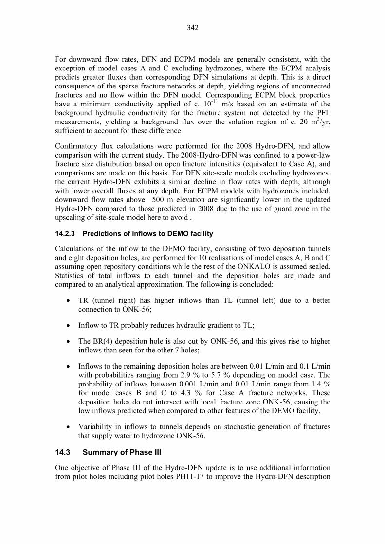
342
For downward flow rates, DFN and ECPM models are generally consistent, with the exception of model cases A and C excluding hydrozones, where the ECPM analysis predicts greater fluxes than corresponding DFN simulations at depth. This is a direct consequence of the sparse fracture networks at depth, yielding regions of unconnected fractures and no flow within the DFN model. Corresponding ECPM block properties have a minimum conductivity applied of c. 10-11 m/s based on an estimate of the background hydraulic conductivity for the fracture system not detected by the PFL measurements, yielding a background flux over the solution region of c. 20 m3/yr, sufficient to account for these difference
Confirmatory flux calculations were performed for the 2008 Hydro-DFN, and allow comparison with the current study. The 2008-Hydro-DFN was confined to a power-law fracture size distribution based on open fracture intensities (equivalent to Case A), and comparisons are made on this basis. For DFN site-scale models excluding hydrozones, the current Hydro-DFN exhibits a similar decline in flow rates with depth, although with lower overall fluxes at any depth. For ECPM models with hydrozones included, downward flow rates above –500 m elevation are significantly lower in the updated Hydro-DFN compared to those predicted in 2008 due to the use of guard zone in the upscaling of site-scale model here to avoid .
14.2.3 Predictions of inflows to DEMO facility
Calculations of the inflow to the DEMO facility, consisting of two deposition tunnels and eight deposition holes, are performed for 10 realisations of model cases A, B and C assuming open repository conditions while the rest of the ONKALO is assumed sealed. Statistics of total inflows to each tunnel and the deposition holes are made and compared to an analytical approximation. The following is concluded:
TR (tunnel right) has higher inflows than TL (tunnel left) due to a better connection to ONK-56;
Inflow to TR probably reduces hydraulic gradient to TL;
The BR(4) deposition hole is also cut by ONK-56, and this gives rise to higher inflows than seen for the other 7 holes;
Inflows to the remaining deposition holes are between 0.01 L/min and 0.1 L/min with probabilities ranging from 2.9 % to 5.7 % depending on model case. The probability of inflows between 0.001 L/min and 0.01 L/min range from 1.4 % for model cases B and C to 4.3 % for Case A fracture networks. These deposition holes do not intersect with local fracture zone ONK-56, causing the low inflows predicted when compared to other features of the DEMO facility.
Variability in inflows to tunnels depends on stochastic generation of fractures that supply water to hydrozone ONK-56.
14.3 Summary of Phase III
One objective of Phase III of the Hydro-DFN update is to use additional information from pilot holes including pilot holes PH11-17 to improve the Hydro-DFN description
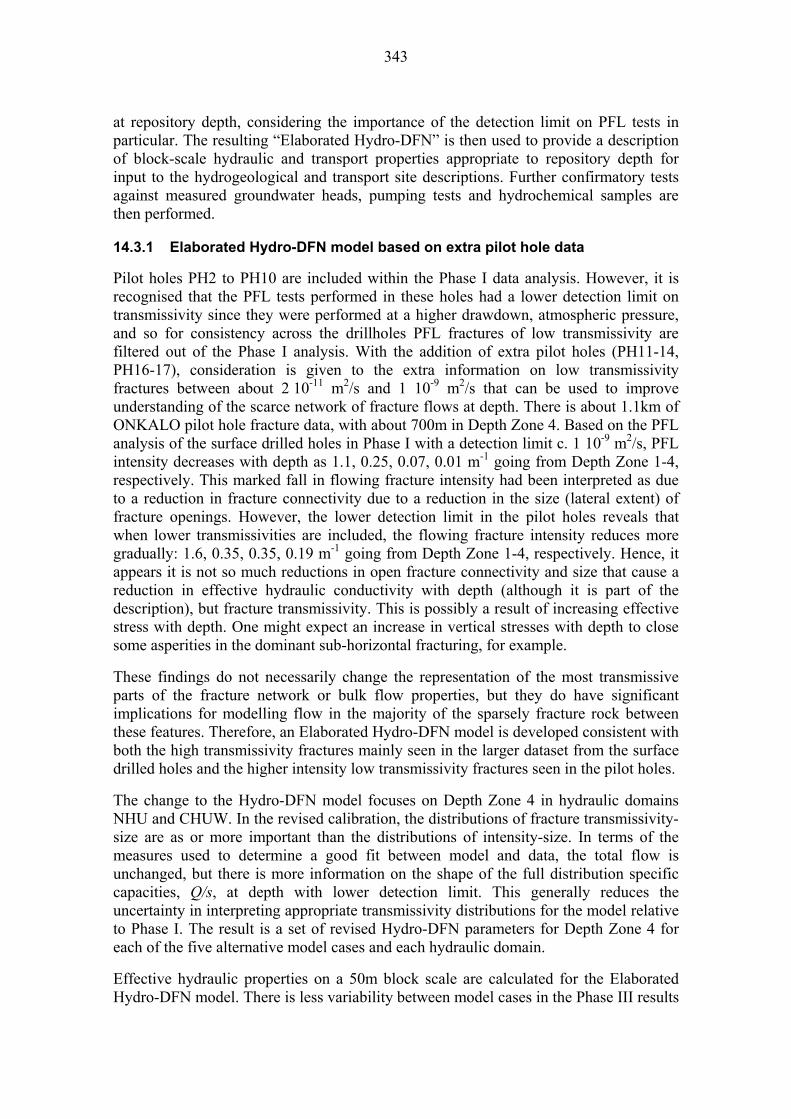
343
at repository depth, considering the importance of the detection limit on PFL tests in particular. The resulting “Elaborated Hydro-DFN” is then used to provide a description of block-scale hydraulic and transport properties appropriate to repository depth for input to the hydrogeological and transport site descriptions. Further confirmatory tests against measured groundwater heads, pumping tests and hydrochemical samples are then performed.
14.3.1 Elaborated Hydro-DFN model based on extra pilot hole data
Pilot holes PH2 to PH10 are included within the Phase I data analysis. However, it is recognised that the PFL tests performed in these holes had a lower detection limit on transmissivity since they were performed at a higher drawdown, atmospheric pressure, and so for consistency across the drillholes PFL fractures of low transmissivity are filtered out of the Phase I analysis. With the addition of extra pilot holes (PH11-14, PH16-17), consideration is given to the extra information on low transmissivity fractures between about 2 10-11 m2/s and 1 10-9 m2/s that can be used to improve understanding of the scarce network of fracture flows at depth. There is about 1.1km of ONKALO pilot hole fracture data, with about 700m in Depth Zone 4. Based on the PFL analysis of the surface drilled holes in Phase I with a detection limit c. 1 10-9 m2/s, PFL intensity decreases with depth as 1.1, 0.25, 0.07, 0.01 m-1 going from Depth Zone 1-4, respectively. This marked fall in flowing fracture intensity had been interpreted as due to a reduction in fracture connectivity due to a reduction in the size (lateral extent) of fracture openings. However, the lower detection limit in the pilot holes reveals that when lower transmissivities are included, the flowing fracture intensity reduces more gradually: 1.6, 0.35, 0.35, 0.19 m-1 going from Depth Zone 1-4, respectively. Hence, it appears it is not so much reductions in open fracture connectivity and size that cause a reduction in effective hydraulic conductivity with depth (although it is part of the description), but fracture transmissivity. This is possibly a result of increasing effective stress with depth. One might expect an increase in vertical stresses with depth to close some asperities in the dominant sub-horizontal fracturing, for example.
These findings do not necessarily change the representation of the most transmissive parts of the fracture network or bulk flow properties, but they do have significant implications for modelling flow in the majority of the sparsely fracture rock between these features. Therefore, an Elaborated Hydro-DFN model is developed consistent with both the high transmissivity fractures mainly seen in the larger dataset from the surface drilled holes and the higher intensity low transmissivity fractures seen in the pilot holes.
The change to the Hydro-DFN model focuses on Depth Zone 4 in hydraulic domains NHU and CHUW. In the revised calibration, the distributions of fracture transmissivity-size are as or more important than the distributions of intensity-size. In terms of the measures used to determine a good fit between model and data, the total flow is unchanged, but there is more information on the shape of the full distribution specific capacities, Q/s, at depth with lower detection limit. This generally reduces the uncertainty in interpreting appropriate transmissivity distributions for the model relative to Phase I. The result is a set of revised Hydro-DFN parameters for Depth Zone 4 for each of the five alternative model cases and each hydraulic domain.
Effective hydraulic properties on a 50m block scale are calculated for the Elaborated Hydro-DFN model. There is less variability between model cases in the Phase III results

344
compared to Phase I, with the geometric mean conductivity around 3 10-11 m/s, similar to typical values in Phase I for DZ4. The standard deviation in the logarithm of hydraulic conductivity is reduced from around 1.0 to 0.5, and the variability between model cases is also half an order of magnitude or less. This reduced variability between model cases is a consequence of the additional PFL data available for the DZ4 calibration in the Phase III analysis, providing greater constraint in the flow calibrations of the different model cases.
14.3.2 Repository-scale transport properties
Flow-related transport properties representative of the bedrock in the repository volume between hydrozones are required as part of the site descriptive modelling. Transport properties are derived here for a generic block-scale of 200m to characterise flow paths in the immediate vicinity of the repository. Transport in each of 3 axial directions are considered for a linear head gradient of 1 % across the 200 m block. The relevant hydraulic sub-domains for the repository are NHU and CHUW within Depth Zone 4. The flow-related transport properties of interest are:
The average Darcy flow-rate per unit width, Qr, (m2/y) in the first fracture the
particle is released in adjacent to the deposition hole;
The cumulative advective travel times, tr, and flow-related transport resistance, Fr, until the particle exits the block;
The percentage of release points (i.e. deposition holes) connected to the fracture network.
The approach to releasing particles is to consider release into the connected network from a 5 by 5 array of synthetic deposition holes with height 7.8 m and diameter 1.75 m spaced 9 m apart. This is more representative of deposition hole geometry than used in the 2008 Hydro-DFN /Hartley et al. 2009/, and considers a smaller release volume as a consequence. 10 particles are released from each deposition hole connected to the network, and 40 realisations are perfumed for each model case.
There is less than half an order of magnitude variation in the median performance measures between the model cases and hydraulic domains NHU and CHUW suggesting that the PFL data strongly constrains the uncertainties in transport properties resulting from uncertain assumptions in the Hydro-DFN model, even though quite different conceptual models are considered. Median flow-related transport resistance is around 107 yr/m; median initial flow-rate per unit width is about 3 10-5 m2/yr; and median advective travel time is around 200 yr. With the uncorrelated size-transmissivity model, the resulting Fr distribution has an extended, albeit small, tail of lower Fr values for both NHU and CHUW. The tail arises in uncorrelated models and possibly in semi-correlated models where small fractures can have large transmissivities giving the potential for higher flow-rates to cascade down to the often small fractures that provide the connection between the deposition holes and the connected fracture network.
The percentage of deposition holes connected to the network varies between about 28 % for Case A, 22 % for Case B, and 31 % for Case C. For CHUW, the values are 23 % for Case A, 20 % for Case B and 25 % for Case C. Since each Case is calibrated against the

345
same average intensity of flowing fractures, one might expect similar percentages for all model cases, and that is more or less the case. The differences between the models in part result from the input intensity of potentially flowing fractures being highest for Case C, then Case A and Case B having the least. That is, although the calibration ensured the connectivity as seen in a linear drillhole are very similar, the connectivity as seen in a fairly dense group of cylindrical deposition holes may be higher when the initial intensity is highest. This seems to have a weak, but nonetheless evident effect here and might be expected to also in safety assessment calculations considering a repository layout.
14.3.3 Site-scale transport properties
Flow-related transport properties on a site-scale are required as part of the site descriptive modelling. Freshwater flow calculations performed using the Elaborated Hydro-DFN model, and subsequent particle tracking analysis yield transport properties of interest. This is an extension of the analysis of transport properties determined on the repository scale as detailed in Chapter 11, although with additional constraints on the model to make simulations computationally tractable. Five realisations of the Case A fracture intensity-size model with semi-correlated transmissivities, and two realisations each of the Case A correlated and uncorrelated, as well as semi-correlated Case B and Case C Hydro-DFN models are considered.
The vast majority of groundwater pathways from the repository volume are shown to exit in the sea to the north of the island, and in the sea to the south of the island. To the south of the island, pathways are bounded by the southerly lineaments, a consequence of the constant high transmissivities (10-5 m2/s) specified for the lineaments in these simulations. To the north, many of the pathways are bounded by the northern lineament BFZ214, although some migrate further, and thought to be a result of BFZ214 being defined with a decreasing transmissivity with depth. It should be noted that in the palaeohydrogeological simulations, described in Section 14.3.5, the depth trend given in Table 3-14 was used instead as it was found a constant transmissivity resulted in deep circulation of meteoric water not seen at the site. A few paths starting from the eastern repository block exit onshore due to the presence of Hydrozone HZ146, which acts as a conduit for particles to travel from repository depth up to the surface.
For Case A, 2 realisations were simulated for each of three size-transmissivity correlations models (5 realisations were simulated for the semi-correlated base case), with the percentage of deposition holes connected to the fracture network ranging from ~36 % for uncorrelated, 24 % - 27 % for semi-correlated and ~22 % for correlated transmissivities. The differences between realisations are about 2 %. These values are consistent with corresponding results in hydraulic domains NHU and CHUW for repository-scale simulations. Comparison of the percentage of deposition holes intersected by the connected network for the three fracture intensity-size models (i.e. Case A, Case B and Case C) with semi-correlated transmissivities are also made. Across realisations, the percentage for Case A ranged from 24.2 % - 27.0 %, for Case B 18.9 % - 22.7 % and for Case C 24.5 % - 28.9 %. Results for both Case A and Case C are in good agreement with the corresponding repository-scale models for domains NHU and CHUW. However, Case B percentages for site-scale analysis are significantly lower than the equivalent repository models, but this is a consequence of the truncation limits
346
on size and transmissivity applied to the site-scale model to make the simulations tractable. We expect that similar results to Cases A and C would be obtained if it were possible to relax these truncation limits.
14.3.4 Site-scale confirmatory analysis
Confirmatory analysis of site-scale models using the Elaborated Hydro-DFN description are performed by comparison with baseline head measurements in a number of drillholes. Infiltration rates to the bedrock are estimated from site-scale flux calculations in Phase II, with 8 mm/yr applied on the top of the bedrock for all model cases considered. Five realisations of the Case A, and two realisations each of the Case B and Case C models are considered, with semi-correlated transmissivity distributions applied. Minor calibration of the transmissivities specified on hydrozones and stochastically generated background fractures are performed to provide more consistent results with observations. Analysis suggests a more transmissive description for the hydrozones, especially at shallow depths, with a factor of four increase above -150 m elevation, a factor of three increase between -150 m and -400 m, and factor of two increase for elevations below -400 m. Background fractures are subsequently adjusted by model case as follows:
Case A: transmissivities in sub-vertical fractures are halved in Depth Zone 1 for all domains;
Case B: All transmissivities in Depth Zone 1 are three times larger;
Case C: All transmissivities in Depth Zone 1 should be doubled.
These changes can be compared with the magnitudes of variability in mean block hydraulic conductivities within Depth Zone 1 between model cases quantified in Table 6-1 through Table 6-4 and Figure 6-3. These imply a variation of 0.5 orders of magnitude between model cases and a standard deviation between blocks of 0.2-0.5 orders of magnitude. Therefore, the adjustments described above are deemed to lie within inherent uncertainties of the model interpretation.
Site-scale models based on the Elaborated Hydro-DFN and the changes described above predicted baseline heads accurately across fifteen drillholes at elevations above -300m, with most measurements realisable across the suite of simulations performed (i.e. they are within the span of values simulated by the generated realisations). Below -300 m, measured heads generally increase due to increasing salinity of groundwater with depth.
Following the baseline head analysis, four pumping tests were simulated using the Elaborated Hydro-DFN. Interference tests offer an insight into the interconnectivity between specific drillholes, with Hydrozones HZ20A, HZ20B, HZ19A, HZ19B and HZ19C dominating connections between the points of abstraction and monitored drillholes. As such hydrozone calibrations, although based on those determined for the preceding baseline head analysis, were extended to background properties of individual hydrozones and the local conditioning values applied.
A suite of steady-state simulations are performed consisting of five realisations of the Case A, and two realisations each of the Case B and Case C models, with transmissivities semi-correlated to fracture size. Results accurately predict the measured
347
drawdowns in the pumped drillhole and most of the monitored drillholes, although for specific test sections large variations in drawdown across realisations are found (c. 8m). Where discrepancies between simulated drawdowns and measurements occur, simulated drawdowns are greater than observations in monitored drillholes. This occurs in a few intervals at short distances, less than 400m from the pumped drillhole, which suggests the models may have too much connectivity in the hydrozones, and indeed when stochastic variability within hydrozones is considered, some realisations show a significantly improved match. Where the discrepancies occur at large distances, greater than 400m from the pumped drillhole, there is an added uncertainty in whether head levels have stabilised over the duration of the pumping test, and so either transient simulations or longer duration tests would be required to address the issues.
In conclusion, it is suggested that moderate changes to the interpreted properties of Hydrozones HZ20A, HZ20B, HZ19A, HZ19B and HZ19C based on single hole tests are necessary to ensure consistency with the pumping tests. Other suggested moderate changes to the transmissivities of the sparsely fractured rock in Depth Zone 1 reflect underling uncertainties in the interpretation of the hydraulic data and are investigated further in the palaeohydrogeological confirmatory tests.
14.3.5 Palaeohydrogeology calculations
Modelling the evolution of the hydrogeological and hydrochemical situation over the last 8000 years (Holocene) provides a means to test the understanding of various parts of the overall site description. Understanding of how palaeo-climate has evolved during the period implies changes to surface topography, sea-level and sea water salinity, and hence changes in boundary conditions on the hydrogeological system. These changes imply changes to the groundwater flow system that in turn will modify groundwater composition through mixing (as well as water-rock interactions) and a density-dependent flow system. Essentially, this provides a natural tracer test of how changes to surface water composition infiltrating the groundwater system result in changes in groundwater composition in the bedrock, the consequences of which are seen in the hydrochemical samples. Clearly, this is not a controlled test as details of initial conditions and changes in boundary conditions are uncertain. Still, it provides a test of the general understanding of the hydrogeological situation as a dynamic system gradual evolving due to changes in climate, and the important parameters and processes that control this system.
The simulations performed assume an initial uniform groundwater composition 8000 years ago based on present-day chemical conditions at depth which are assumed to have changed very little, along with an assumed mix of Brine and Glacial Waters and a relic Subglacial water in the upper bedrock. Changes due to the evolution of boundary conditions for groundwater flow and surface water composition, such as the Littorina period, are modelled as the mixing of five different references waters, defined in terms of the mass fractions of major ions and environmental isotopes. The transport equations include advection, dispersion and rock matrix diffusion and are implemented in an ECPM model. The bedrock hydraulic properties are obtained from upscaling the elaborated Hydro-DFN along with a representation of the hydrozones. A representation of the overburden is also included since it has a significant control on recharge to the bedrock.
348
The resulting groundwater heads and composition in drillholes for present-day conditions are compared with baseline data. A series of sensitivity variants have been used in order to identify the key parameters determining groundwater mixing. After calibration of the recharge and overburden properties, a reasonable agreement with baseline heads across the Olkiluoto site is obtained. Considering this result together with the findings of the confirmatory tests on baseline heads for DFN simulations described in Section 14.3.4, suggests that measured groundwater heads can be reproduced by either slightly increasing transmissivities in the upper bedrock or by including a representation of the overburden with an average hydraulic conductivity of 10-4 m/s. The simulations of groundwater components such as chloride, sulphate and bicarbonate are also in reasonable agreement, although Meteoric water is found to penetrate too deep in some model variants. Sensitivity analysis indicates that key parameters are the bedrock hydraulic conductivity in the top 100 m and the fracture surface area, affecting both the rate of rock matrix diffusion and the depth into the matrix that can accessed in a given time, and hence retardation of the mixing front.
Stochastic uncertainties in groundwater head and chemical composition were analysed by simulating multiple realisations of the palaeohydrogeological ECPM model. Three fracture intensity-size models Case A, B and C were considered with semi-correlated transmissivities applied. For Case A, correlated and uncorrelated transmissivity distributions were also evaluated. Sensitivity of groundwater head predictions to realisation was limited with similar profiles obtained for all model cases considered. Groundwater concentrations of sulphate and bicarbonate were also predicted, with results illustrating a greater sensitivity to model realisation. The envelope of just five model realisations captures many of the sampled data suggesting some of the overall model description is consistent with the data, although individual sampled measurements probably result from local heterogeneity in hydraulic properties. Some of the variability in measurements in the near-surface is likely only explained by variability in near-surface chemical processes. There is some possible significance that the simulated infiltration profile for Altered meteoric water (indicated by bicarbonate) and Littorina water (indicated by sulphate) are closer to observations for Cases B and C compared to Case A. This is thought to be due to the slightly higher hydraulic conductivity in hydraulic domain CHUW, in the centre of the island, for Depth Zones 1 and 2 (see Figure 7-12); the result of which is also seen in the gross flow-rates shown in Figure 8-3, for example.
The consequences for palaeohydrogeological simulations of present-day heads and hydrochemistry of the changes to hydrozone properties suggested by the Hydro-DFN calibration to the pumping tests described in Section 14.3.4 were assessed as a sensitivity variant. The changes to transmissivity of Hydrozones HZ099, HZ19A/B/C and HZ20A/B suggested by simulations of the cross-hole tests for pumping in KR1, KR4, KR7 and KR8 made little change to the palaeohydrogeological results relative to the base case simulations where the hydrozones are parameterised according to the interpretation of single-hole PFL tests. This suggests that local changes to hydrozone properties, typically increases of half an order of magnitude, necessary to simulate the cross-hole tests make little difference to the distributions of head and hydrochemistry. Hence, the changes can be considered as model variants to reflect uncertainty in hydraulic conditions within hydrozones local to some drillhole, but these are unlikely to effect wider flow and solute transport conditions.

349
REFERENCES
Aaltonen, I (ed.), Lahti M, Engström J, Mattila J, Paananen M, Paulamäki S, Gehör S, Kärki A, Ahokas T, Torvela T and Front K, 2010. Geological Model of the Olkiluoto Site, Version 2. Posiva Working Report WR 2010-70.
Ahokas H, Vaittinen T, Tammisto E, Nummela J, 2007. Modelling of hydro zones for the layout planning and numerical flow model in 2006. Working Report 2007-01, Posiva Oy, Eurajoki.
Ahokas H, Tammisto E and Lehtimäki T, 2008. Baseline Head in Olkiluoto. Working Report 2008-69. Posiva Oy. Olkiluoto.
Bingham C, 1974. An antipodally symmetric distribution on the sphere, Annals of Statistics v. 2, pp. 1201-1225.
Buoro A, Dahlbo K, Wiren L, Holmén J, Hermanson J, and Fox A (ed.), 2009. Geological Discrete-Fracture Network Model (version 1) for the Olkiluoto Site, Finland, Working Report 2009-77, Posiva Oy, Eurajoki, Finland.
Eronen M, Glückert G, van de Plassche O, van de Plicht J and Rantala P, 1995. Land uplift in the Olkiluoto-Pyhäjärvi area, southwestern Finland, during last 8000 years. Waste Commission of Finnish Power Companies, Helsinki, Finland. Report YJT-95-17.
Eronen, M. and Lehtinen, K., 1996. Description of the Quaternary geological history of Romuvaara, Kivetty and Olkiluoto sites (in Finnish with an English abstract). Posiva Working Report PATU-96-74.
Follin S, Levén J, Hartley L, Jackson P, Joyce S, Roberts D, Swift B, 2007. Hydrogeological characterisation and modelling of deformation zones and fracture domains, Forsmark model stage 2.2. SKB R-07-48, Svensk Kärnbränslehantering AB.
Fox A, et al. 2011. Geological Discrete-Fracture Network Model (version 2) for the Olkiluoto Site, Finland, Working Report 2011-XX, Posiva Oy, Eurajoki, Finland.
Hartikainen J, Hartikainen K, Hautojärvi A, Kuoppamäki K and Timonen J, 1996. Helium gas methods for rock characteristics and matrix diffusion. Report Posiva 96-22.
Hartley L, Hoek J, Swan D, Roberts D, Joyce D, Follin S. 2009. Development of a hydrogeological discrete fracture network model for the Olkiluoto site descriptive model 2008. Posiva Working Report 2009-61, Posiva Oy.
Hartley L, Hoek J, Swan D, Roberts D, 2010. Hydrogeological discrete fracture network modelling of groundwater flow under open repository conditions. Posiva Working Report 2010-51, Posiva Oy.
Hjerne C, Nordqvist R, and Harrström J, 2010. Compilation and analyses of results from cross-hole tracer tests with conservative tracers. SKB Report R-09-28.
350
Hoch A, Jackson C P, 2004. Rock-matrix diffusion in transport of salinity. Implementation in CONNECTFLOW. SKB R-04-78. Svensk Kärnbränslehantering AB.
Hämäläinen, 2011. Monitoring Hydraulic Conductivity with HTU at Eurajoki, Olkiluoto, Drillholes OL-KR31 and OL-KR32, in 2010. Posiva Working Report 2011-49, Posiva Oy.
Jackson CP, Hoch AR and Todman SJ, 2000. Self-consistency of a heterogeneous continuum porous medium representation of a fractured medium, Water Resources Research Vol 36. No 1, Pages 189-202.
Karvonen T, 2008. Surface and Near-Surface Hydrological Model of Olkiluoto Island. Posiva Report 2008-17.
Karvonen T, 2011, Olkiluoto Surface and Near-Surface Hydrological Modelling in 2010. Posiva Report 2011-50.
Kestin J, Khalifa H E, Correia R J, 1981. Tables of dynamic and kinematic viscosity of aqueous NaCl solutions in the temperature range 20 -150 0C and the pressure range 0.1-35 Mpa. J. Phys. Chem. Ref. Data Vol 10, No 1.
Laaksoharju M, Smellie J, Tullborg E-L, Gimeno M., Molinero, J, Gurban I, and Hallbeck, L, 2008. Hydrogeochemical evaluation and modelling performed within the Swedish site investigation programme. Applied Geochemistry 23, 1761-1795.
Löfman J, Mészáros F, Keto V, Pitkänen P, Ahokas H, 2009. Modelling of groundwater flow and solute transport in Olkiluoto – Update 2008. Working Report 2009-78. Posiva Oy. Olkiluoto.
Löfman J, Poteri A, 2009. Groundwater flow and transport simulations in support of RNT-2008 analysis, Posiva Working Report 2008-52, Posiva Oy.
Mattila J, Aaltonen I, Kemppainen K, Wikström L, Paananen M, Paulamäki S, Front K, Gehör S, Kärki A, Ahokas T, 2008. Geological model of the Olkiluoto site, Version 1.0, Working Report 2007-92, Posiva Oy, Eurajoki.
Mattila, J, 2009. Constraints on the fault and fracture evolution at the Olkiluoto region. Posiva Working Report 2009-130.
Munier R, Hökmark H, 2004. Respect distances: Rationale and means of computation, Report R-04-17. Svensk Kärnbränslehantering AB (SKB), Stockholm, Sweden.
Paananen M and Paulamäki S, 1995. Preceding Geological and Petrophysical Modelling of the Drill Hole OL-KR10, Olkiluoto Study Site, Eurajoki, Southwestern Finland. Work Report PATU-95-65, TVO, Helsinki. (In Finnish).
Paulamäki S and Paananen M, 1995. Preceding Geological and Petrophysical Modelling of the Extended Part of the Drill Hole OL-KR2, Olkiluoto Study Site, Eurajoki, Southwestern Finland. Work Report PATU-95-49, TVO, Helsinki. (In Finnish).
351
Pitkänen P, Partamies S and Luukkonen A, 2004. Hydrogeochemical interpretation of baseline groundwater conditions at the Olkiluoto site. Posiva Report 2003-07.
Pitkänen P, Ahokas H, Ylä-Mella M, Partamies S, Snellman M, Hellä P, 2007. Quality Review of Hydrochemical Baseline Data from the Olkiluoto Site. Posiva Working Report 2007-05, Posiva Oy.
Partamies S, and Pitkänen, P, 2012. Massbalance modelling results of groundwater data collected at Olkiluoto in 2004 - 2007. Posiva Working Report 2012-XX (in prep.), Posiva Oy.
Posiva, 2009. Olkiluoto site description 2008. Posiva Oy, POSIVA 2009-01.
Posiva, 2011. Olkiluoto site description 2011. Posiva Oy, POSIVA 2011-02.
Remes H, Kuula H, Somervuori P, and Hakala M, 2009. ONKALO rock mechanics model (RMM) - Version 1.0, Working Report 2009-55, Posiva Oy, Olkiluoto, Finland.
Rhén I, Forsmark T, Hartley L, Jackson P; Roberts D, Swan D, Gylling B, 2008, Hydrogeological conceptualisation and parameterisation. Site descriptive modelling SDM-Site Laxemar, Report R-08-78. Svensk Kärnbränslehantering AB (SKB), Stockholm, Sweden.
Rocscience, 2010, Dips Version 5.1 - Graphical and Statistical Analysis of Orientation Data. www.rocscience.com, Toronto, Ontario, Canada.
ESRI, 2010, ArcView 9.2. www.esri.com, Environmental Systems Research Institute, Redlands, California, USA.
Serco, 2010a, ConnectFlow Release 10.0, Technical Summary Document, Serco report SA/ENV/CONNECTFLOW/15.
Serco, 2010b, NAMMU Release 10.0 Technical Summary Document, Serco report SA/ENV/CONNECTFLOW/8.
Serco, 2010c, NAPSAC Release 10.0 Technical Summary Document, Serco report SA/ENV/CONNECTFLOW/12.
Serco, 2011, ConnectFlow Verification, Serco report SERCO/001015.18/001.
Salonen, V.-P., Eronen M. and Saarnisto, M., 2002. Käytännön maaperägeologia (in Finnish). Kirja-Aurora, Turku, p. 237.
Sokolnicki M and Rouhiainen P, 2005. Difference flow logging of drillholes KLX07A and KLX07B, Subarea Laxemar, Oskarshamn site investigation. SKB P-05-225, Svensk Kärnbränslehantering AB.
Tammisto E, Palmén J and Ahokas H, 2009. Database for hydraulically conductive fractures. Posiva Working Report 2009-30, Posiva Oy.

352
Tammisto E, and Palmén J, 2011. Database for Hydraulically Conductive Fractures – Update 2010. Posiva Working Report 2011-12, Posiva Oy.
Tanaka H, 1999. Circular asymmetry of the paleomagnetic directions observed at low latitude volcanic sites. Earth, Planets and Space (51).
Tauxe L, 2010. Essentials of Paleomagnetism. University of California Press, 2010.
Terzaghi R, 1965. Sources of error in joint surveys. Geotechnique 15(3): 287-304.
Thiem G, 1906 Hydrologische Methoden, Gebhardt, Leipzig, pp. 56.
Vaittinen T, Nummela J and Ahokas H, 2008. Compilation and analysis of hydrogeological responses to field activities in Olkiluoto. Posiva Working Report 2008-03, Posiva Oy.
Vaittinen T, Ahokas H, Nummela J, 2009. Hydrogeological structure model of the Olkiluoto Site – update in 2008. Posiva Working Report 2009-15, Posiva Oy.
Vaittinen T, Ahokas H, Nummela J, and Paulamäki, S, 2011. Hydrogeological structure model of the Olkiluoto Site – update in 2010. Posiva Working Report 2011-65, Posiva Oy.
Westman P, Wastegård S, Schoning K and Gustafsson B, 1999. Salinity changes in the Baltic Sea during the last 8500 years, causes and models. TR-99-38. Svensk Kärnbränslehantering AB.
353
APPENDIX A: MERGING HYDRAULIC DOMAINS
Nine domains were identified in the Geo-DFN model, based on tectonic subdomains defined in the Olkiluoto ductile deformation model that are assumed to be the base rock volumes within which the geological fracture model is built /Fox et al. 2011/. These nine domains were:
Northern (NTU)
Southern (STU)
Central 1 (CTU1)
Central 2 (CTU2)
Central 3 (CTU3)
Selkänummi SZ (SDZ)
D3 Deformation (FSZ)
Liikla SZ (LSZ)
D4-1 (D4)
All the domains above have different characteristics, but there may also be many characteristics of each domain which may be shared with other domains. Here, we investigate the similarities between each of the domains to determine the scope for merging together the nine domains above into a smaller number of larger domains.
A.1 Merging hydraulic domains
The criteria used to assess the suitability for merging domains together is given below:
Geographic location – domains should be adjacent;
Stereoplot orientation data – stereoplots should display similar character characteristics in terms of the fracture orientations and major concentrations;
fracture intensity by fracture set – the relative P10,corr values for each set in each of the domains should have similar relative values;
fracture intensity data by depth – these should have similar P10,corr intensities with a similar depth profile;
hydraulic conductivity – these should display similar profiles for conductivity by depth.
It should be noted that the merging of domains is based on the fracture database and does not include enhancements to the PFL or fracture data as described in Section 3.2.3.
Fracture intensity by depth plots and domain for all fractures and PFL fractures are shown in Appendix B; hydraulic conductivity plots by depth for each domain are shown

354
in Appendix C and stereoplots for all fractures and PFL fractures by domain are shown in Appendix D. Fracture intensities by fracture set for each domain for all fractures and PFL fractures are shown in Figure A-1 and Figure A-2 below.
Fracture intensity by Set and fracture domain outside of HZ
0
0.5
1
1.5
2
2.5
CTU1 CTU2 CTU3 D4 FSZ LSZ NTU SDZ STU
Fracture Domain
P10
,Co
rr (
m-1
)
N-S E-W SH
Figure A-1. Fracture intensities for all fractures outside hydrozones by domain and fracture set.
PFL intensity by Set and fracture domain outside of HZ
0
0.05
0.1
0.15
0.2
0.25
0.3
0.35
CTU1 CTU2 CTU3 D4 FSZ LSZ NTU SDZ STU
Fracture Domain
P10
,Co
rr (
m-1
)
N-S E-W SH
Figure A-2. Intensities for PFL fractures outside hydrozones by domain and fracture set.
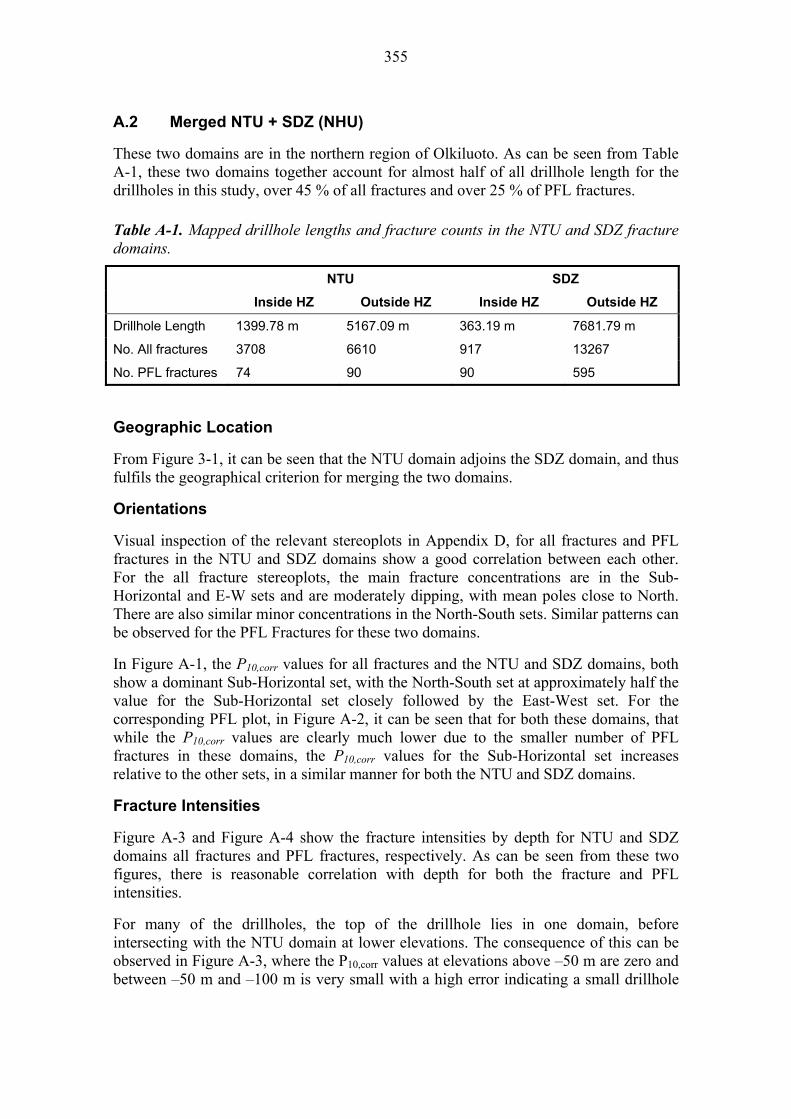
355
A.2 Merged NTU + SDZ (NHU)
These two domains are in the northern region of Olkiluoto. As can be seen from Table A-1, these two domains together account for almost half of all drillhole length for the drillholes in this study, over 45 % of all fractures and over 25 % of PFL fractures.
Table A-1. Mapped drillhole lengths and fracture counts in the NTU and SDZ fracture domains.
NTU SDZ
Inside HZ Outside HZ Inside HZ Outside HZ
Drillhole Length 1399.78 m 5167.09 m 363.19 m 7681.79 m
No. All fractures 3708 6610 917 13267
No. PFL fractures 74 90 90 595
Geographic Location
From Figure 3-1, it can be seen that the NTU domain adjoins the SDZ domain, and thus fulfils the geographical criterion for merging the two domains.
Orientations
Visual inspection of the relevant stereoplots in Appendix D, for all fractures and PFL fractures in the NTU and SDZ domains show a good correlation between each other. For the all fracture stereoplots, the main fracture concentrations are in the Sub-Horizontal and E-W sets and are moderately dipping, with mean poles close to North. There are also similar minor concentrations in the North-South sets. Similar patterns can be observed for the PFL Fractures for these two domains.
In Figure A-1, the P10,corr values for all fractures and the NTU and SDZ domains, both show a dominant Sub-Horizontal set, with the North-South set at approximately half the value for the Sub-Horizontal set closely followed by the East-West set. For the corresponding PFL plot, in Figure A-2, it can be seen that for both these domains, that while the P10,corr values are clearly much lower due to the smaller number of PFL fractures in these domains, the P10,corr values for the Sub-Horizontal set increases relative to the other sets, in a similar manner for both the NTU and SDZ domains.
Fracture Intensities
Figure A-3 and Figure A-4 show the fracture intensities by depth for NTU and SDZ domains all fractures and PFL fractures, respectively. As can be seen from these two figures, there is reasonable correlation with depth for both the fracture and PFL intensities.
For many of the drillholes, the top of the drillhole lies in one domain, before intersecting with the NTU domain at lower elevations. The consequence of this can be observed in Figure A-3, where the P10,corr values at elevations above –50 m are zero and between –50 m and –100 m is very small with a high error indicating a small drillhole
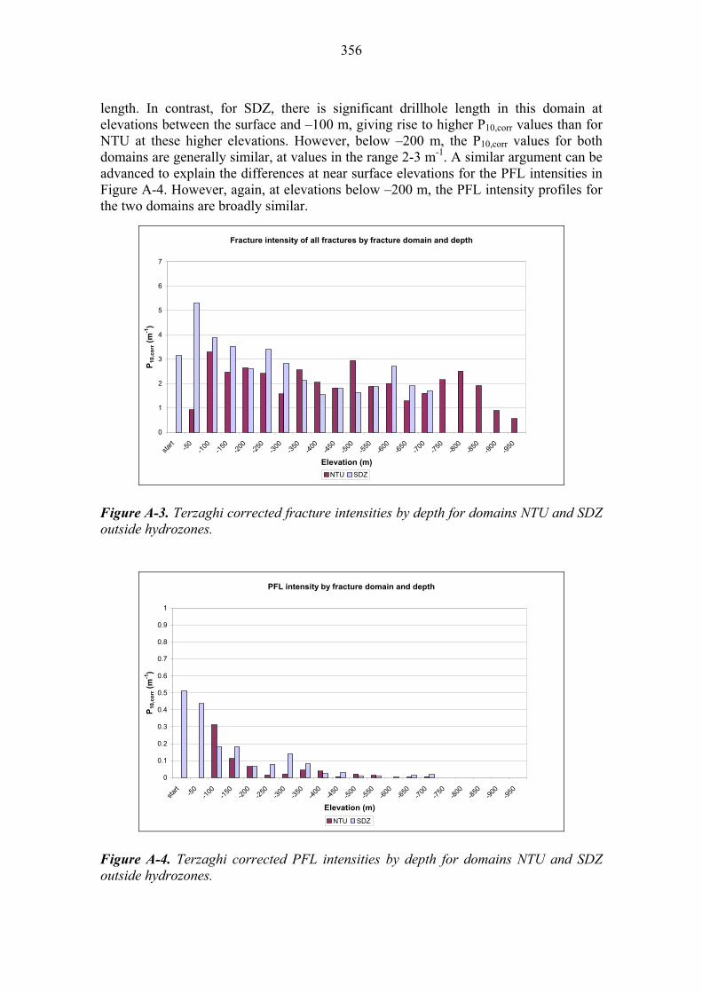
356
length. In contrast, for SDZ, there is significant drillhole length in this domain at elevations between the surface and –100 m, giving rise to higher P10,corr values than for NTU at these higher elevations. However, below –200 m, the P10,corr values for both domains are generally similar, at values in the range 2-3 m-1. A similar argument can be advanced to explain the differences at near surface elevations for the PFL intensities in Figure A-4. However, again, at elevations below –200 m, the PFL intensity profiles for the two domains are broadly similar.
Fracture intensity of all fractures by fracture domain and depth
0
1
2
3
4
5
6
7
start
-50
-100
-150
-200
-250
-300
-350
-400
-450
-500
-550
-600
-650
-700
-750
-800
-850
-900
-950
Elevation (m)
P10
,co
rr (
m-1
)
NTU SDZ
Figure A-3. Terzaghi corrected fracture intensities by depth for domains NTU and SDZ outside hydrozones.
PFL intensity by fracture domain and depth
0
0.1
0.2
0.3
0.4
0.5
0.6
0.7
0.8
0.9
1
start
-50
-100
-150
-200
-250
-300
-350
-400
-450
-500
-550
-600
-650
-700
-750
-800
-850
-900
-950
Elevation (m)
P10
,co
rr (
m-1
)
NTU SDZ
Figure A-4. Terzaghi corrected PFL intensities by depth for domains NTU and SDZ outside hydrozones.

357
Hydraulic Conductivities
Figure A-5 shows that profiles of effective hydraulic conductivity with depth are also consistent between NTU and SDZ.
Hydraulic conductivity by fracture domain and depth
1.E-11
1.E-10
1.E-09
1.E-08
1.E-07
1.E-06
start
-50
-100
-150
-200
-250
-300
-350
-400
-450
-500
-550
-600
-650
-700
-750
-800
-850
-900
-950
Elevation (m)
L (
m/s
)
NTU SDZ
Figure A-5. Hydraulic conductivities by depth for domains NTU and SDZ outside hydrozones.
A.2 Merged CTU1 + CTU2 + FSZ (CHUW)
This is another major domain when merged containing about 40 % of all drillhole length and fractures and over 53 % of PFL fractures (see Table A-2).
Table A-2. Mapped drillhole lengths and fracture counts in the CTU1, CTU2 and FSZ fracture domains.
CTU1 CTU2 FSZ
Inside HZ Outside HZ Inside HZ Outside HZ Inside HZ Outside HZ
Drillhole Length
765.04 m 2908.17 m 638.17 m 6286.28 m 301.50 m 946.26 m
No. all fractures
1828 5304 2301 10163 788 1506
No. PFL fractures
177 525 200 675 36 125
358
Geographic Location
From Figure 3-1 it can be seen that the CTU1, CTU2 and FSZ domains each adjoin each other, and thus fulfils the geographical criterion for merging the 3 domains.
Orientations
Visual inspection of the stereonets for all fractures and PFL fractures in Appendix D show a reasonable correlation between the three domains. For the all fracture stereonets, for all three domains the main fracture concentrations are in the Sub-Horizontal and E-W sets and are gently to moderately dipping, with mean poles of between 320 and north. All three domains also show some minor concentrations in the North-South and East-West sets. Although with a smaller number of poles, similar patterns can be observed for the PFL Fractures for these three domains.
In Figure A-1, the fracture intensities for all fractures in the CTU1, CTU2 and FSZ domains respectively show a dominant Sub-Horizontal set, with the North-South set at approximately one third the value for the Sub-Horizontal set closely followed by the East-West set. For the corresponding PFL plot, in Figure A-2, it can be seen that for each of these three domains, that while the P10,corr values are clearly much lower due to the smaller number of PFL fractures in these domains, the P10,corr values for the Sub-Horizontal set increases relative to the other sets, in a similar manner for each of the CTU1, CTU2 and FSZ domains.
Fracture Intensities
Figure A-6 and Figure A-7 show the fracture intensities by depth for CTU1, CTU2 and FSZ, respectively, for all fractures and PFL fractures.
These two figures indicate that there is broad agreement between these domains down to around –300 m, although it can be seen that at elevations below –400 m, fracture intensities are only found in the CTU2 domain. However, for PFL fractures this difference between the domains is less apparent (mainly because the PFL fractures do not extend beyond -450 m) and the thus agreement between the domains is much better.

359
Fracture intensity of all fractures by fracture domain and depth
0
1
2
3
4
5
6
7
start
-50
-100
-150
-200
-250
-300
-350
-400
-450
-500
-550
-600
-650
-700
-750
-800
-850
-900
-950
Elevation (m)
P10
corr (
m-1
)
CTU1 CTU2 FSZ
Figure A-6. Terzaghi corrected fracture intensities for domain CTU1, CTU2 and FSZ outside hydrozones.
PFL intensity by fracture domain and depth
0
0.1
0.2
0.3
0.4
0.5
0.6
0.7
0.8
0.9
1
start
-50
-100
-150
-200
-250
-300
-350
-400
-450
-500
-550
-600
-650
-700
-750
-800
-850
-900
-950
Elevation (m)
P10
,co
rr (
m-1
)
CTU1 CTU2 FSZ
Figure A-7. Terzaghi corrected PFL intensities for domains CTU1, CTU2 and FSZ outside hydrozones.
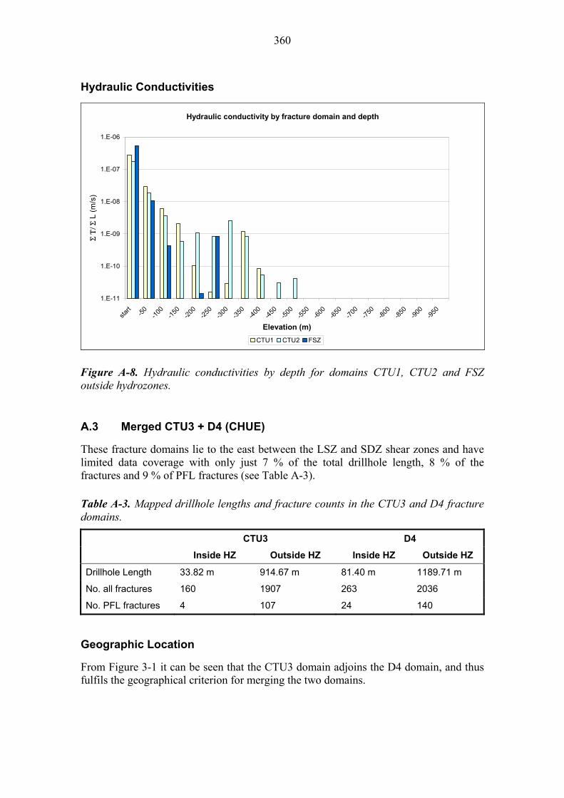
360
Hydraulic Conductivities
Hydraulic conductivity by fracture domain and depth
1.E-11
1.E-10
1.E-09
1.E-08
1.E-07
1.E-06
start
-50
-100
-150
-200
-250
-300
-350
-400
-450
-500
-550
-600
-650
-700
-750
-800
-850
-900
-950
Elevation (m)
L (
m/s
)
CTU1 CTU2 FSZ
Figure A-8. Hydraulic conductivities by depth for domains CTU1, CTU2 and FSZ outside hydrozones.
A.3 Merged CTU3 + D4 (CHUE)
These fracture domains lie to the east between the LSZ and SDZ shear zones and have limited data coverage with only just 7 % of the total drillhole length, 8 % of the fractures and 9 % of PFL fractures (see Table A-3).
Table A-3. Mapped drillhole lengths and fracture counts in the CTU3 and D4 fracture domains.
CTU3 D4
Inside HZ Outside HZ Inside HZ Outside HZ
Drillhole Length 33.82 m 914.67 m 81.40 m 1189.71 m
No. all fractures 160 1907 263 2036
No. PFL fractures 4 107 24 140
Geographic Location
From Figure 3-1 it can be seen that the CTU3 domain adjoins the D4 domain, and thus fulfils the geographical criterion for merging the two domains.

361
Orientations
Visual inspection of the stereonets for all fractures and PFL fractures in Appendix D show a reasonable correlation between the two domains. For the all fracture stereonets, for both domains the main fracture concentrations are in the Sub-Horizontal and E-W/N-W border sets and are moderately to steeply dipping, with mean poles of approximately 315 degrees. Both domains also show some minor concentrations in the North-South set. Although with a smaller number of poles, similar patterns can be observed for the PFL Fractures in D4, although, it is conceded that the stereonet for PFL fractures in CTU3 is inconclusive, mainly due to the lack of poles within this domain.
In Figure A-1, the fracture intensities for all fractures in the CTU3 and D4 domains respectively show a dominant Sub-Horizontal set, with the East-West set at approximately one third the value for the Sub-Horizontal set closely followed by the North-South set. For the corresponding PFL plot, in Figure A-2, it can be seen that for both these domains, that while the P10,corr values are clearly much lower due to the smaller number of PFL fractures in these domains, the P10,corr values for the Sub-Horizontal set decreases relative to the other sets in CTU3.
Fracture Intensities
Figure A-9 and Figure A-10 show the fracture intensities by depth for CTU3 and D4 for all fractures and PFL fractures, respectively. From these two figures, it can be seen that there is a reasonable agreement for both all fractures and PFL fractures in elevations down to approximately -200 m. At lower depths, there are greater differences, but there is low statistical significance for PFL fractures in particular.
Fracture intensity of all fractures by fracture domain and depth
0
1
2
3
4
5
6
7
start
-50
-100
-150
-200
-250
-300
-350
-400
-450
-500
-550
-600
-650
-700
-750
-800
-850
-900
-950
Elevation (m)
P10
corr (
m-1
)
CTU3 D4
Figure A-9. Terzaghi corrected fracture intensities for domains CTU3 and D4 outside hydrozones.
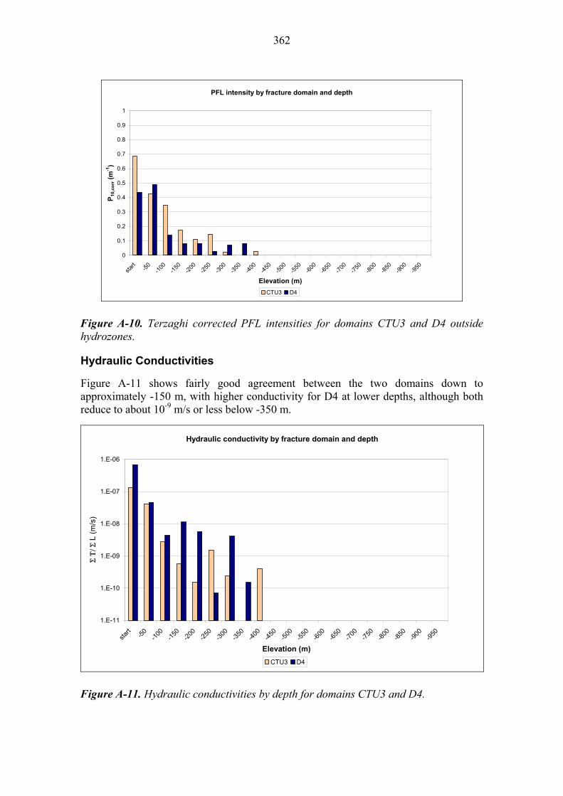
362
PFL intensity by fracture domain and depth
0
0.1
0.2
0.3
0.4
0.5
0.6
0.7
0.8
0.9
1
star
t-5
0-1
00-1
50-2
00-2
50-3
00-3
50-4
00-4
50-5
00-5
50-6
00-6
50-7
00-7
50-8
00-8
50-9
00-9
50
Elevation (m)
P10
,co
rr (
m-1
)
CTU3 D4
Figure A-10. Terzaghi corrected PFL intensities for domains CTU3 and D4 outside hydrozones.
Hydraulic Conductivities
Figure A-11 shows fairly good agreement between the two domains down to approximately -150 m, with higher conductivity for D4 at lower depths, although both reduce to about 10-9 m/s or less below -350 m.
Hydraulic conductivity by fracture domain and depth
1.E-11
1.E-10
1.E-09
1.E-08
1.E-07
1.E-06
start
-50
-100
-150
-200
-250
-300
-350
-400
-450
-500
-550
-600
-650
-700
-750
-800
-850
-900
-950
Elevation (m)
L (
m/s
)
CTU3 D4
Figure A-11. Hydraulic conductivities by depth for domains CTU3 and D4.
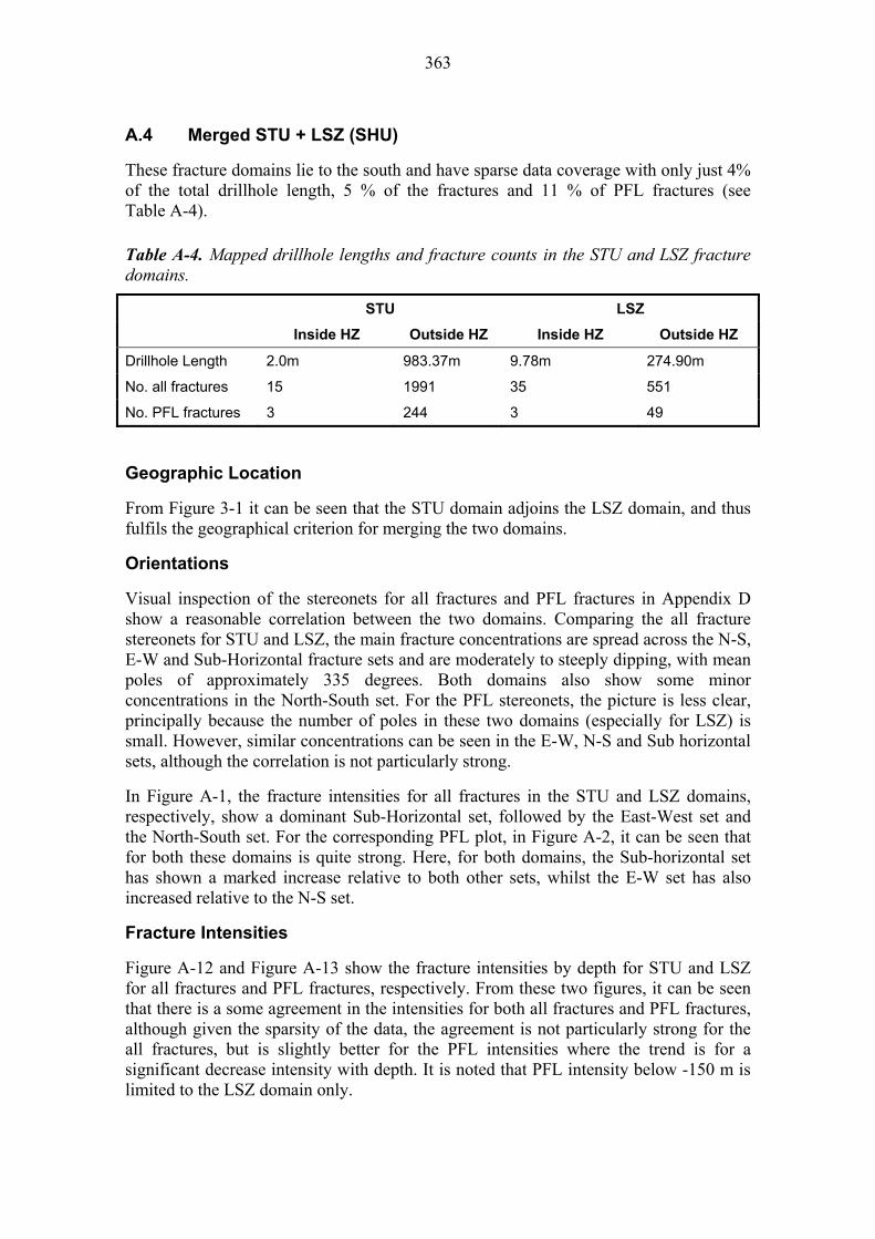
363
A.4 Merged STU + LSZ (SHU)
These fracture domains lie to the south and have sparse data coverage with only just 4% of the total drillhole length, 5 % of the fractures and 11 % of PFL fractures (see Table A-4).
Table A-4. Mapped drillhole lengths and fracture counts in the STU and LSZ fracture domains.
STU LSZ
Inside HZ Outside HZ Inside HZ Outside HZ
Drillhole Length 2.0m 983.37m 9.78m 274.90m
No. all fractures 15 1991 35 551
No. PFL fractures 3 244 3 49
Geographic Location
From Figure 3-1 it can be seen that the STU domain adjoins the LSZ domain, and thus fulfils the geographical criterion for merging the two domains.
Orientations
Visual inspection of the stereonets for all fractures and PFL fractures in Appendix D show a reasonable correlation between the two domains. Comparing the all fracture stereonets for STU and LSZ, the main fracture concentrations are spread across the N-S, E-W and Sub-Horizontal fracture sets and are moderately to steeply dipping, with mean poles of approximately 335 degrees. Both domains also show some minor concentrations in the North-South set. For the PFL stereonets, the picture is less clear, principally because the number of poles in these two domains (especially for LSZ) is small. However, similar concentrations can be seen in the E-W, N-S and Sub horizontal sets, although the correlation is not particularly strong.
In Figure A-1, the fracture intensities for all fractures in the STU and LSZ domains, respectively, show a dominant Sub-Horizontal set, followed by the East-West set and the North-South set. For the corresponding PFL plot, in Figure A-2, it can be seen that for both these domains is quite strong. Here, for both domains, the Sub-horizontal set has shown a marked increase relative to both other sets, whilst the E-W set has also increased relative to the N-S set.
Fracture Intensities
Figure A-12 and Figure A-13 show the fracture intensities by depth for STU and LSZ for all fractures and PFL fractures, respectively. From these two figures, it can be seen that there is a some agreement in the intensities for both all fractures and PFL fractures, although given the sparsity of the data, the agreement is not particularly strong for the all fractures, but is slightly better for the PFL intensities where the trend is for a significant decrease intensity with depth. It is noted that PFL intensity below -150 m is limited to the LSZ domain only.
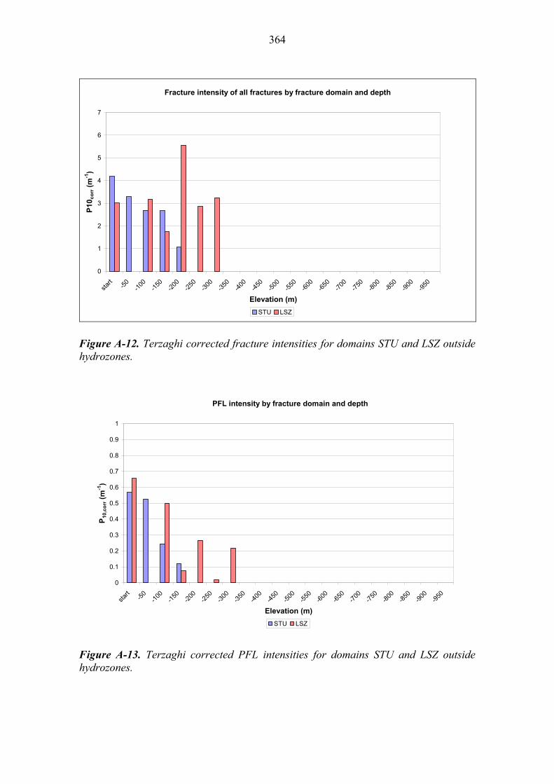
364
Fracture intensity of all fractures by fracture domain and depth
0
1
2
3
4
5
6
7
start
-50
-100
-150
-200
-250
-300
-350
-400
-450
-500
-550
-600
-650
-700
-750
-800
-850
-900
-950
Elevation (m)
P10
corr (
m-1
)
STU LSZ
Figure A-12. Terzaghi corrected fracture intensities for domains STU and LSZ outside hydrozones.
PFL intensity by fracture domain and depth
0
0.1
0.2
0.3
0.4
0.5
0.6
0.7
0.8
0.9
1
start
-50
-100
-150
-200
-250
-300
-350
-400
-450
-500
-550
-600
-650
-700
-750
-800
-850
-900
-950
Elevation (m)
P10
,co
rr (
m-1
)
STU LSZ
Figure A-13. Terzaghi corrected PFL intensities for domains STU and LSZ outside hydrozones.

365
Hydraulic Conductivities
Figure A-14 shows reasonable agreement between the two domains down to approximately -150 m. At depths below -150 m, only conductivity is limited to the LSZ domain only.
Hydraulic conductivity by fracture domain and depth
1.E-11
1.E-10
1.E-09
1.E-08
1.E-07
1.E-06
start
-50
-100
-150
-200
-250
-300
-350
-400
-450
-500
-550
-600
-650
-700
-750
-800
-850
-900
-950
Elevation (m)
L (
m/s
)
STU LSZ
Figure A-14. Hydraulic conductivities by depth for domains STU and LSZ.

366
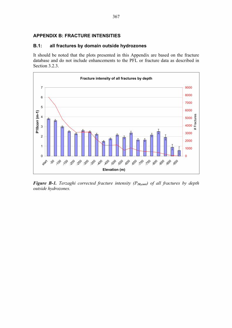
367
APPENDIX B: FRACTURE INTENSITIES
B.1: all fractures by domain outside hydrozones
It should be noted that the plots presented in this Appendix are based on the fracture database and do not include enhancements to the PFL or fracture data as described in Section 3.2.3.
Fracture intensity of all fractures by depth
0
1
2
3
4
5
6
7
start
-50
-100
-150
-200
-250
-300
-350
-400
-450
-500
-550
-600
-650
-700
-750
-800
-850
-900
-950
Elevation (m)
P10
corr
(m
-1)
0
1000
2000
3000
4000
5000
6000
7000
8000
9000
# F
ract
ures
Figure B-1. Terzaghi corrected fracture intensity (P10,corr) of all fractures by depth outside hydrozones.

368
Fracture intensity of all fractures in NTU by depth
0
1
2
3
4
5
6
7
start
-50
-100
-150
-200
-250
-300
-350
-400
-450
-500
-550
-600
-650
-700
-750
-800
-850
-900
-950
Elevation (m)
P10
corr
(m
-1)
0
100
200
300
400
500
600
700
# F
ract
ures
Figure B-2. Terzaghi corrected fracture intensity (P10,corr) of all fractures by depth for domain NTU outside hydrozones.
Fracture intensity of all fractures in STU by depth
0
1
2
3
4
5
6
7
start
-50
-100
-150
-200
-250
-300
-350
-400
-450
-500
-550
-600
-650
-700
-750
-800
-850
-900
-950
Elevation (m)
P10
co
rr (
m-1
)
0
100
200
300
400
500
600
700
# F
ract
ures
Figure B-3. Terzaghi corrected fracture intensity (P10,corr) of all fractures by depth for domain STU outside hydrozones.

369
Fracture intensity of all fractures in CTU1 by depth
0
1
2
3
4
5
6
7
start
-50
-100
-150
-200
-250
-300
-350
-400
-450
-500
-550
-600
-650
-700
-750
-800
-850
-900
-950
Elevation (m)
P10
corr
(m
-1)
0
200
400
600
800
1000
1200
1400
1600
1800
2000
# F
ract
ures
Figure B-4. Terzaghi corrected fracture intensity (P10,corr) of all fractures by depth for domain CTU1 outside hydrozones.
Fracture intensity of all fractures in CTU2 by depth
0
1
2
3
4
5
6
7
start
-50
-100
-150
-200
-250
-300
-350
-400
-450
-500
-550
-600
-650
-700
-750
-800
-850
-900
-950
Elevation (m)
P10
co
rr (
m-1
)
0
500
1000
1500
2000
2500
3000
3500
# F
ract
ures
Figure B-5. Terzaghi corrected fracture intensity (P10,corr) of all fractures by depth for domain CTU2 outside hydrozones.

370
Fracture intensity of all fractures in CTU3 by depth
0
1
2
3
4
5
6
7
start
-50
-100
-150
-200
-250
-300
-350
-400
-450
-500
-550
-600
-650
-700
-750
-800
-850
-900
-950
Elevation (m)
P10
corr
(m
-1)
0
50
100
150
200
250
300
350
# F
ract
ures
Figure B-6. Terzaghi corrected fracture intensity (P10,corr) of all fractures by depth for domain CTU3 outside hydrozones.
Fracture intensity of all fractures in SDZ by depth
0
1
2
3
4
5
6
7
start
-50
-100
-150
-200
-250
-300
-350
-400
-450
-500
-550
-600
-650
-700
-750
-800
-850
-900
-950
Elevation (m)
P10
corr
(m
-1)
0
500
1000
1500
2000
2500
# F
ract
ures
Figure B-7. Terzaghi corrected fracture intensity (P10,corr) of all fractures by depth for domain SDZ outside hydrozones.
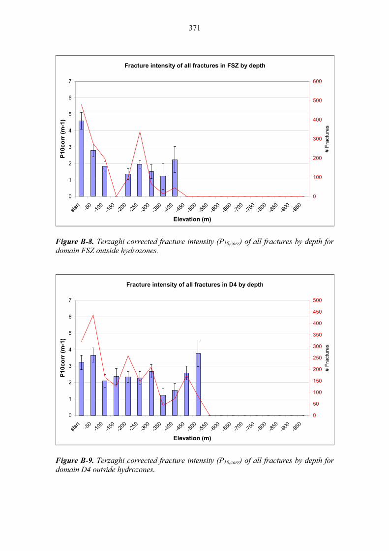
371
Fracture intensity of all fractures in FSZ by depth
0
1
2
3
4
5
6
7
start
-50
-100
-150
-200
-250
-300
-350
-400
-450
-500
-550
-600
-650
-700
-750
-800
-850
-900
-950
Elevation (m)
P10
corr
(m
-1)
0
100
200
300
400
500
600
# F
ract
ures
Figure B-8. Terzaghi corrected fracture intensity (P10,corr) of all fractures by depth for domain FSZ outside hydrozones.
Fracture intensity of all fractures in D4 by depth
0
1
2
3
4
5
6
7
start
-50
-100
-150
-200
-250
-300
-350
-400
-450
-500
-550
-600
-650
-700
-750
-800
-850
-900
-950
Elevation (m)
P10
corr
(m
-1)
0
50
100
150
200
250
300
350
400
450
500
# F
ract
ures
Figure B-9. Terzaghi corrected fracture intensity (P10,corr) of all fractures by depth for domain D4 outside hydrozones.

372
Fracture intensity of all fractures in LSZ by depth
0
1
2
3
4
5
6
7
start
-50
-100
-150
-200
-250
-300
-350
-400
-450
-500
-550
-600
-650
-700
-750
-800
-850
-900
-950
Elevation (m)
P10
corr
(m
-1)
0
20
40
60
80
100
120
140
# F
ract
ure
s
Figure B-10. Terzaghi corrected fracture intensity (P10,corr) of all fractures by depth for domain LSZ outside hydrozones.
B.2: PFL Fractures by domain outside hydrozones
PFL intensity by depth
0
0.1
0.2
0.3
0.4
0.5
0.6
0.7
0.8
0.9
1
start
-50
-100
-150
-200
-250
-300
-350
-400
-450
-500
-550
-600
-650
-700
-750
-800
-850
-900
-950
Elevation (m)
P10
corr
(m
-1)
0
200
400
600
800
1000
1200
# F
ract
ures
Figure B-11. Terzaghi corrected fracture intensity (P10,corr) of PFL fractures by depth for all domains outside hydrozones.

373
PFL intensity in NTU by depth
0
0.1
0.2
0.3
0.4
0.5
0.6
0.7
0.8
0.9
1
start
-50
-100
-150
-200
-250
-300
-350
-400
-450
-500
-550
-600
-650
-700
-750
-800
-850
-900
-950
Elevation (m)
P10
corr
(m
-1)
0
5
10
15
20
25
# F
ract
ures
Figure B-12. Terzaghi corrected fracture intensity (P10,corr) of PFL fractures by depth for domain NTU outside hydrozones.
PFL intensity in CTU1 by depth
0
0.1
0.2
0.3
0.4
0.5
0.6
0.7
0.8
0.9
1
start
-50
-100
-150
-200
-250
-300
-350
-400
-450
-500
-550
-600
-650
-700
-750
-800
-850
-900
-950
Elevation (m)
P10
corr
(m
-1)
0
50
100
150
200
250
300
# F
ract
ure
s
Figure B-13. Terzaghi corrected fracture intensity (P10,corr) of PFL fractures by depth for domain CTU1 outside hydrozones.
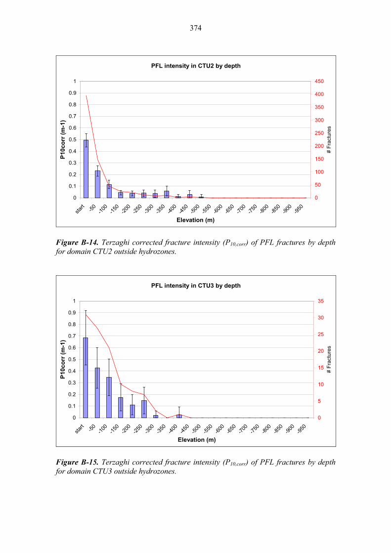
374
PFL intensity in CTU2 by depth
0
0.1
0.2
0.3
0.4
0.5
0.6
0.7
0.8
0.9
1
start
-50
-100
-150
-200
-250
-300
-350
-400
-450
-500
-550
-600
-650
-700
-750
-800
-850
-900
-950
Elevation (m)
P10
corr
(m
-1)
0
50
100
150
200
250
300
350
400
450
# F
ract
ures
Figure B-14. Terzaghi corrected fracture intensity (P10,corr) of PFL fractures by depth for domain CTU2 outside hydrozones.
PFL intensity in CTU3 by depth
0
0.1
0.2
0.3
0.4
0.5
0.6
0.7
0.8
0.9
1
start
-50
-100
-150
-200
-250
-300
-350
-400
-450
-500
-550
-600
-650
-700
-750
-800
-850
-900
-950
Elevation (m)
P10
corr
(m
-1)
0
5
10
15
20
25
30
35
# F
ract
ure
s
Figure B-15. Terzaghi corrected fracture intensity (P10,corr) of PFL fractures by depth for domain CTU3 outside hydrozones.

375
PFL intensity in STU by depth
0
0.1
0.2
0.3
0.4
0.5
0.6
0.7
0.8
0.9
1
start
-50
-100
-150
-200
-250
-300
-350
-400
-450
-500
-550
-600
-650
-700
-750
-800
-850
-900
-950
Elevation (m)
P10
co
rr (
m-1
)
0
20
40
60
80
100
120
# F
ract
ures
Figure B-16. Terzaghi corrected fracture intensity (P10,corr) of PFL fractures by depth for domain STU outside hydrozones.
PFL intensity in SDZ by depth
0
0.1
0.2
0.3
0.4
0.5
0.6
0.7
0.8
0.9
1
start
-50
-100
-150
-200
-250
-300
-350
-400
-450
-500
-550
-600
-650
-700
-750
-800
-850
-900
-950
Elevation (m)
P10
corr
(m
-1)
0
20
40
60
80
100
120
140
160
# F
ract
ure
s
Figure B-17. Terzaghi corrected fracture intensity (P10,corr) of PFL fractures by depth for domain SDZ outside hydrozones.

376
PFL intensity in FSZ by depth
0
0.1
0.2
0.3
0.4
0.5
0.6
0.7
0.8
0.9
1
start
-50
-100
-150
-200
-250
-300
-350
-400
-450
-500
-550
-600
-650
-700
-750
-800
-850
-900
-950
Elevation (m)
P10
corr
(m
-1)
0
10
20
30
40
50
60
70
80
# F
ract
ures
Figure B-18. Terzaghi corrected fracture intensity (P10,corr) of PFL fractures by depth for domain FSZ outside hydrozones.
PFL intensity in D4 by depth
0
0.1
0.2
0.3
0.4
0.5
0.6
0.7
0.8
0.9
1
start
-50
-100
-150
-200
-250
-300
-350
-400
-450
-500
-550
-600
-650
-700
-750
-800
-850
-900
-950
Elevation (m)
P10
corr
(m
-1)
0
10
20
30
40
50
60
# F
ract
ure
s
Figure B-19. Terzaghi corrected fracture intensity (P10,corr) of PFL fractures by depth for domain D4 outside hydrozones.

377
PFL intensity in LSZ by depth
0
0.1
0.2
0.3
0.4
0.5
0.6
0.7
0.8
0.9
1
start
-50
-100
-150
-200
-250
-300
-350
-400
-450
-500
-550
-600
-650
-700
-750
-800
-850
-900
-950
Elevation (m)
P10
corr
(m
-1)
0
5
10
15
20
25
30
# F
ract
ures
Figure B-20. Terzaghi corrected fracture intensity (P10,corr) of PFL fractures by depth for domain LSZ outside hydrozones.
B.3: Intensities inside hydrozones
Fracture intensity of all fractures by depth in HZ
0
1
2
3
4
5
6
7
start
-50
-100
-150
-200
-250
-300
-350
-400
-450
-500
-550
-600
-650
-700
-750
-800
-850
-900
-950
Elevation (m)
P10
corr
(m
-1)
0
200
400
600
800
1000
1200
1400
# F
ract
ures
Figure B-21. Terzaghi corrected fracture intensity (P10,corr) of all fractures by depth inside hydrozones.

378
Fracture intensity of PFL fractures by depth in HZ
0
0.1
0.2
0.3
0.4
0.5
0.6
0.7
0.8
0.9
1
start
-50
-100
-150
-200
-250
-300
-350
-400
-450
-500
-550
-600
-650
-700
-750
-800
-850
-900
-950
Elevation (m)
P10
corr
(m
-1)
0
20
40
60
80
100
120
140
160
180
# F
ract
ures
Figure B-22. Terzaghi corrected fracture intensity (P10,corr) of PFL fractures by depth inside hydrozones.
B.4: Indicative error bars
In the plots of fracture intensity shown above and in Chapter 4, indicative error bars are shown to give an idea of the statistical errors. The error bars correspond to 2 standard deviations either side of the central value. For a normal distribution with a known variance, this range is close to a 95 % confidence interval for the mean. The distributions in question are not normal, but for long lengths of drillhole intersected by many fractures, the distributions will be approximately normal from the law of large numbers. However, a precise statistical significance is not attached to the error bars. Rather they are simply used to give a visual indication of the relative magnitudes of the errors.
The standard deviations were estimated from the available data on the basis that the fractures are randomly distributed in space i.e. are not clustered, that is correspond to independent samples from a simple Poisson distribution, and have distributions of size and orientation that are independent and independent of position. In this case, it can be shown that, for example, for circular fractures the expectation (mean) of the number of fractures intersected by a vertical drillhole of length L is given by
LrDrDdddrn r
cos),()(sin 22
0
2
00
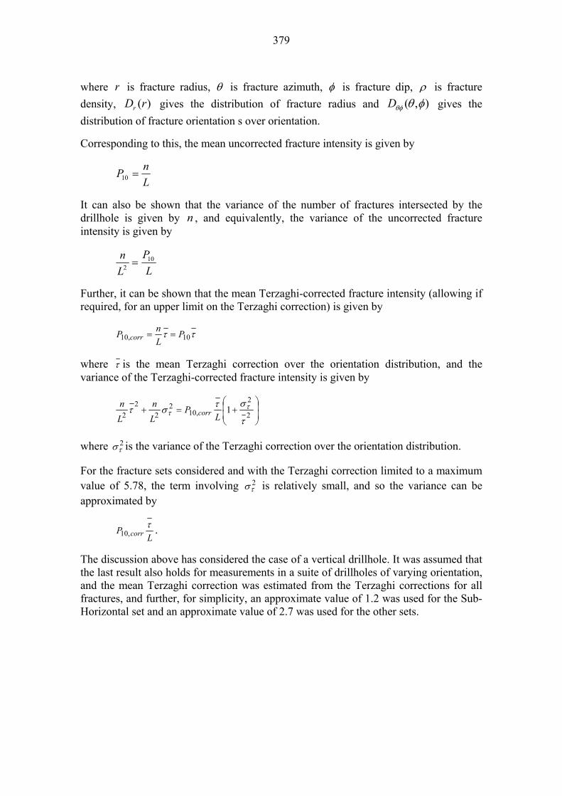
379
where r is fracture radius, is fracture azimuth, is fracture dip, is fracture
density, )(rDr gives the distribution of fracture radius and ),( D gives the
distribution of fracture orientation s over orientation.
Corresponding to this, the mean uncorrected fracture intensity is given by
L
nP 10
It can also be shown that the variance of the number of fractures intersected by the drillhole is given by n , and equivalently, the variance of the uncorrected fracture intensity is given by
L
P
L
n 102
Further, it can be shown that the mean Terzaghi-corrected fracture intensity (allowing if required, for an upper limit on the Terzaghi correction) is given by
10,10 PL
nP corr
where is the mean Terzaghi correction over the orientation distribution, and the variance of the Terzaghi-corrected fracture intensity is given by
2
2
,102
2
2
21
L
PL
n
L
ncorr
where 2 is the variance of the Terzaghi correction over the orientation distribution.
For the fracture sets considered and with the Terzaghi correction limited to a maximum value of 5.78, the term involving 2
is relatively small, and so the variance can be approximated by
LP corr
,10 .
The discussion above has considered the case of a vertical drillhole. It was assumed that the last result also holds for measurements in a suite of drillholes of varying orientation, and the mean Terzaghi correction was estimated from the Terzaghi corrections for all fractures, and further, for simplicity, an approximate value of 1.2 was used for the Sub-Horizontal set and an approximate value of 2.7 was used for the other sets.

380

381
APPENDIX C: HYDRAULIC CONDUCTIVITIES
C.1: Hydraulic conductivities by domain outside hydrozones
It should be noted that plots presented in this Appendix are based on the fracture database and do not include enhancements to the PFL or fracture data as described in 3.2.3.
Hydraulic conductivity by depth
1.E-11
1.E-10
1.E-09
1.E-08
1.E-07
1.E-06
start
-50
-100
-150
-200
-250
-300
-350
-400
-450
-500
-550
-600
-650
-700
-750
-800
-850
-900
-950
Elevation (m)
∑T
/ ∑
L (
m/s
)
Figure C-1. Average hydraulic conductivity by depth based on sum of PFL interpreted transmissivities divided by length for all domains outside hydrozones.
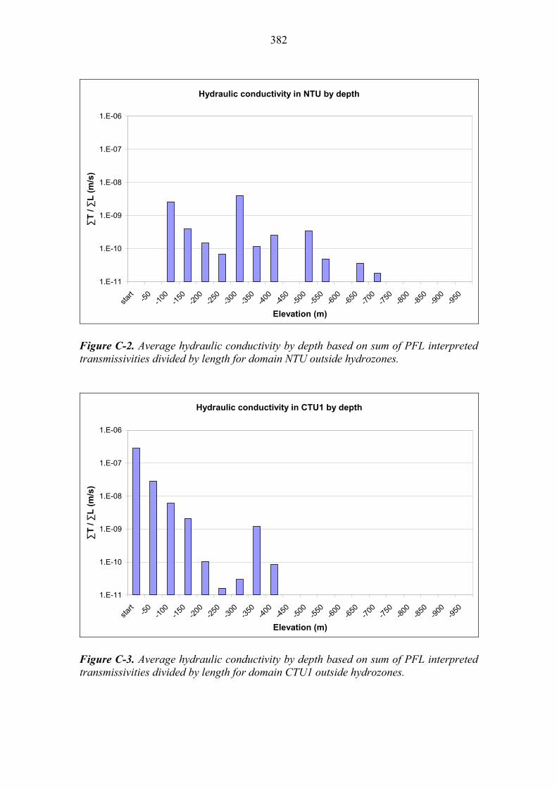
382
Hydraulic conductivity in NTU by depth
1.E-11
1.E-10
1.E-09
1.E-08
1.E-07
1.E-06
start
-50
-100
-150
-200
-250
-300
-350
-400
-450
-500
-550
-600
-650
-700
-750
-800
-850
-900
-950
Elevation (m)
∑T
/ ∑
L (
m/s
)
Figure C-2. Average hydraulic conductivity by depth based on sum of PFL interpreted transmissivities divided by length for domain NTU outside hydrozones.
Hydraulic conductivity in CTU1 by depth
1.E-11
1.E-10
1.E-09
1.E-08
1.E-07
1.E-06
start
-50
-100
-150
-200
-250
-300
-350
-400
-450
-500
-550
-600
-650
-700
-750
-800
-850
-900
-950
Elevation (m)
∑T
/ ∑
L (
m/s
)
Figure C-3. Average hydraulic conductivity by depth based on sum of PFL interpreted transmissivities divided by length for domain CTU1 outside hydrozones.

383
Hydraulic conductivity in CTU2 by depth
1.E-11
1.E-10
1.E-09
1.E-08
1.E-07
1.E-06
start
-50
-100
-150
-200
-250
-300
-350
-400
-450
-500
-550
-600
-650
-700
-750
-800
-850
-900
-950
Elevation (m)
∑T
/ ∑
L (
m/s
)
Figure C-4. Average hydraulic conductivity by depth based on sum of PFL interpreted transmissivities divided by length for domain CTU2 outside hydrozones.
Hydraulic conductivity in CTU3 by depth
1.E-11
1.E-10
1.E-09
1.E-08
1.E-07
1.E-06
start
-50
-100
-150
-200
-250
-300
-350
-400
-450
-500
-550
-600
-650
-700
-750
-800
-850
-900
-950
Elevation (m)
∑T
/ ∑
L (
m/s
)
Figure C-5. Average hydraulic conductivity by depth based on sum of PFL interpreted transmissivities divided by length for domain CTU3 outside hydrozones.

384
Hydraulic conductivity in STU by depth
1.E-11
1.E-10
1.E-09
1.E-08
1.E-07
1.E-06
start
-50
-100
-150
-200
-250
-300
-350
-400
-450
-500
-550
-600
-650
-700
-750
-800
-850
-900
-950
Elevation (m)
∑T
/ ∑
L (
m/s
)
Figure C-6. Average hydraulic conductivity by depth based on sum of PFL interpreted transmissivities divided by length for domain STU outside hydrozones.
Hydraulic conductivity in SDZ by depth
1.E-11
1.E-10
1.E-09
1.E-08
1.E-07
1.E-06
start
-50
-100
-150
-200
-250
-300
-350
-400
-450
-500
-550
-600
-650
-700
-750
-800
-850
-900
-950
Elevation (m)
∑T
/ ∑
L (
m/s
)
Figure C-7. Average hydraulic conductivity by depth based on sum of PFL interpreted transmissivities divided by length for domain SDZ outside hydrozones.
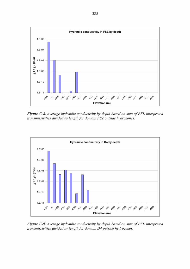
385
Hydraulic conductivity in FSZ by depth
1.E-11
1.E-10
1.E-09
1.E-08
1.E-07
1.E-06
start
-50
-100
-150
-200
-250
-300
-350
-400
-450
-500
-550
-600
-650
-700
-750
-800
-850
-900
-950
Elevation (m)
∑T
/ ∑
L (
m/s
)
Figure C-8. Average hydraulic conductivity by depth based on sum of PFL interpreted transmissivities divided by length for domain FSZ outside hydrozones.
Hydraulic conductivity in D4 by depth
1.E-11
1.E-10
1.E-09
1.E-08
1.E-07
1.E-06
start
-50
-100
-150
-200
-250
-300
-350
-400
-450
-500
-550
-600
-650
-700
-750
-800
-850
-900
-950
Elevation (m)
∑T
/ ∑
L (
m/s
)
Figure C-9. Average hydraulic conductivity by depth based on sum of PFL interpreted transmissivities divided by length for domain D4 outside hydrozones.

386
Hydraulic conductivity in LSZ by depth
1.E-11
1.E-10
1.E-09
1.E-08
1.E-07
1.E-06
start
-50
-100
-150
-200
-250
-300
-350
-400
-450
-500
-550
-600
-650
-700
-750
-800
-850
-900
-950
Elevation (m)
∑T
/ ∑
L (
m/s
)
Figure C-10. Average hydraulic conductivity by depth based on sum of PFL interpreted transmissivities divided by length for domain LSZ outside hydrozones.
C.2: Hydraulic conductivities inside hydrozones
Hydraulic conductivity by depth in HZ
1.E-11
1.E-10
1.E-09
1.E-08
1.E-07
1.E-06
1.E-05
1.E-04
start
-50
-100
-150
-200
-250
-300
-350
-400
-450
-500
-550
-600
-650
-700
-750
-800
-850
-900
-950
Elevation (m)
∑T
/ ∑
L (m
/s)
Figure C-11. Average hydraulic conductivity by depth based on sum of PFL interpreted transmissivities divided by length inside hydrozones.
387
APPENDIX D: STEREONET PLOTS
D:1 All fractures
It should be noted that the stereonet plots presented in this Appendix are based on the fracture database and do not include enhancements to the PFL or fracture data as described in Section 3.2.3.
All Fractures outside HZ
Figure D-1. Stereonet plot for all fractures in all domains outside hydrozones.
All Fractures in NTU outside HZ
Figure D-2. Stereonet plot for all fractures in domain NTU outside hydrozones.
388
All Fractures in CTU1 outside HZ
Figure D-3. Stereonet plot for all fractures in domain CTU1 outside hydrozones.
All Fractures in CTU2 outside HZ
Figure D-4. Stereonet plot for all fractures in domain CTU2 outside hydrozones.
389
All Fractures in CTU3 outside HZ
Figure D-5. Stereonet plot for all fractures in domain CTU3 outside hydrozones.
All Fractures in STU outside HZ
Figure D-6. Stereonet plot for all fractures in domain STU outside hydrozones.
390
All Fractures in SDZ outside HZ
Figure D-7. Stereonet plot for all fractures in domain SDZ outside hydrozones.
All Fractures in FSZ outside HZ
Figure D-8. Stereonet plot for all fractures in domain FSZ outside hydrozones.
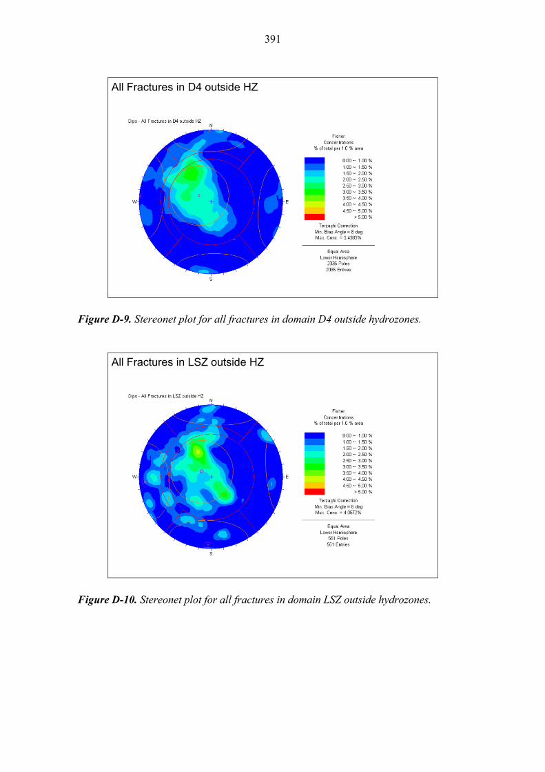
391
All Fractures in D4 outside HZ
Figure D-9. Stereonet plot for all fractures in domain D4 outside hydrozones.
All Fractures in LSZ outside HZ
Figure D-10. Stereonet plot for all fractures in domain LSZ outside hydrozones.

392
D.2: PFL fractures
All PFLs outside HZ
Figure D-11. Stereonet plot for PFL fractures in all domains outside hydrozones.
All PFLs in NTU outside HZ
Figure D-12. Stereonet plot for PFL fractures in domain NTU outside hydrozones.
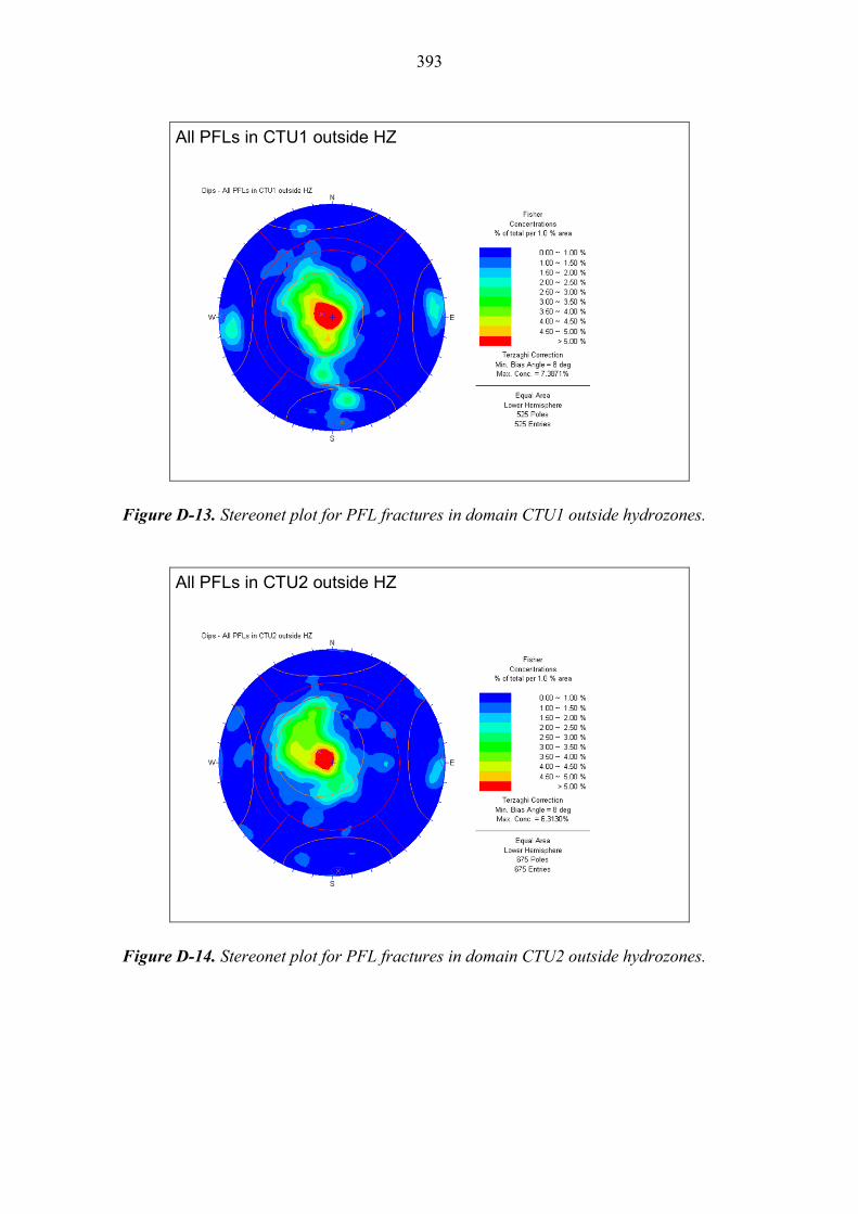
393
All PFLs in CTU1 outside HZ
Figure D-13. Stereonet plot for PFL fractures in domain CTU1 outside hydrozones.
All PFLs in CTU2 outside HZ
Figure D-14. Stereonet plot for PFL fractures in domain CTU2 outside hydrozones.

394
All PFLs in CTU3 outside HZ
Figure D-15. Stereonet plot for PFL fractures in domain CTU3 outside hydrozones.
All PFLs in STU outside HZ
Figure D-16. Stereonet plot for PFL fractures in domain STU outside hydrozones.
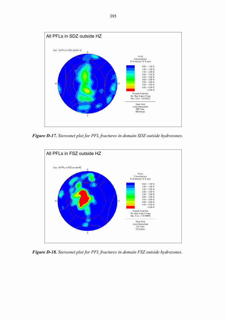
395
All PFLs in SDZ outside HZ
Figure D-17. Stereonet plot for PFL fractures in domain SDZ outside hydrozones.
All PFLs in FSZ outside HZ
Figure D-18. Stereonet plot for PFL fractures in domain FSZ outside hydrozones.

396
All PFLs in D4 outside HZ
Figure D-19. Stereonet plot for PFL fractures in domain D4 outside hydrozones.
All PFLs in LSZ outside HZ
Figure D-20. Stereonet plot for PFL fractures in domain LSZ outside hydrozones.

397
APPENDIX E: DEPTH ZONES FOR INDIVIDUAL DRILLHOLES
Table E-1. Elevations of first and last fracture and PFL fracture in the fracture database for each drillhole.
Drillhole Elevation of
deepest fracture (m)
Elevation of shallowest fracture (m)
Elevation of deepest PFL fracture (m)
Elevation of shallowest PFL
fracture (m) KR1 -916.9 -29.0 -710.1 -30.8 KR10 -600.6 -31.3 -549.1 -31.5 KR11 -877.0 -35.0 -556.3 -108.5 KR12 -761.9 -29.2 -717.3 -30.6 KR13 -410.0 2.8 -402.4 -5.1 KR14 -469.8 2.4 -435.9 -2.0 KR15 -505.1 -32.2 -439.9 -32.7 KR15B -36.7 5.5 -33.8 -2.4 KR16 -160.8 -33.1 -143.7 -33.2 KR16B -35.9 4.8 -31.4 -6.5 KR17 -147.2 -31.5 -123.1 -32.7 KR17B -36.9 5.4 -33.3 0.1 KR18 -115.1 -31.3 -96.2 -31.8 KR18B -36.2 8.9 -32.1 -0.8 KR19 -509.8 -33.2 -468.7 -33.7 KR19B -37.5 3.7 -25.4 -1.0 KR2 -976.3 -30.5 -594.2 -32.7 KR20 -384.4 -23.9 -363.6 -25.8 KR20B -26.6 6.2 -22.0 0.3 KR21 -144.4 6.3 -115.5 -9.6 KR22 -410.2 -27.1 -358.4 -27.7 KR22B -31.9 -0.9 -28.3 -10.9 KR23 -241.2 -26.8 -191.1 -28.0 KR23B -29.3 2.4 -27.5 -0.8 KR24 -539.8 8.3 -413.2 -14.0 KR25 -567.1 -30.8 -539.4 -36.4 KR25B -34.0 4.6 -27.2 -2.7 KR26 -53.6 14.1 -51.1 -5.0 KR27 -424.0 -25.3 -395.8 -26.9 KR27B -25.3 -1.1 -22.3 -1.1 KR28 -415.8 -18.5 -413.0 -18.5 KR28B -20.2 13.2 KR29 -715.5 -30.7 -551.2 -31.5 KR29B -34.7 5.8 -26.2 3.2 KR3 -446.1 -30.5 -419.2 -31.9 KR30 -84.4 5.9 -79.2 -4.9 KR31 -295.3 -29.6 -295.3 -31.8 KR31B -33.0 1.8 -28.6 -2.1 KR32 -150.5 -1.7 -147.6 -10.5 KR33 -226.6 -29.8 -185.6 -29.8 KR33B -31.0 0.3 -22.5 -2.4 KR34 -90.7 5.2 -72.9 -0.1 KR35 -92.4 6.4 -87.6 2.7 KR36 -163.9 8.1 -152.4 1.9 KR37 -240.4 -23.9 -188.2 -27.4 KR37B -28.0 3.2 -24.2 -0.3 KR38 -513.4 6.4 -394.5 -13.2 KR39 -427.6 -28.6 -346.8 -28.6 KR39B -33.1 6.9 -28.6 3.0 KR4 -856.0 -30.0 -820.7 -39.3

398
KR40 -911.0 -33.4 -747.5 -36.4 KR40B -38.0 0.4 -31.0 -1.4 KR41 -357.7 -33.5 -348.3 -35.3 KR41B -38.6 0.1 -34.5 -2.2 KR42 -367.2 -32.5 -311.3 -34.5 KR42B -35.6 3.9 -28.9 -0.5 KR43 -803.2 -21.8 -357.7 -22.4 KR43B -26.2 9.5 -20.9 -0.4 KR44 -721.6 -29.3 -650.9 -31.5 KR44B -31.3 2.5 -28.0 -1.1 KR45 -832.4 -30.4 -502.8 -33.4 KR45B -34.3 2.7 -31.3 -1.9 KR46 -554.7 -33.4 -529.9 -35.1 KR46B -37.0 0.2 KR47 -809.0 -32.6 -576.6 -32.6 KR47B KR48 -518.9 8.7 -411.5 -18.6 KR49 -798.2 -29.1 -285.0 -29.9 KR5 -478.3 -27.3 -409.1 -28.6 KR50 -894.5 -34.7 -684.8 -39.2 KR50B -35.7 -0.1 -32.1 -3.4 KR51 -520.2 -27.1 -469.9 -40.1 KR52 -403.7 -31.8 -364.1 -32.9 KR52B -29.4 4.8 KR53 -209.9 -27.2 -199.9 -27.9 KR53B -32.4 4.1 -28.5 -2.9 KR6 -471.7 -2.0 -411.0 -9.3 KR7 -749.7 7.7 -381.4 -11.8 KR8 -529.9 10.2 -493.4 -7.8 KR9 -540.4 -32.9 -512.3 -33.3 PH10 -346.4 -325.9 -338.0 -335.0 PH2 -19.4 -7.0 -19.0 -7.5 PH3 -76.1 -60.0 -75.6 -61.7 PH4 -86.6 -77.4 -85.0 -79.7 PH5 -107.9 -88.2 -106.1 -93.6 PH6 -142.5 -128.2 -142.0 -129.0 PH7 -180.7 -174.2 -175.1 -174.6 PH8 -306.3 -291.8 -306.2 -292.4 PH9 -321.6 -306.8 -311.6 -307.1

399
Table E-2. Depth Zones determined for individual drillholes. Where the Upper Limit and the Lower Limit are blank, then the drillhole makes no contribution within that particular depth zone.
Drillhole Depth Zone 1 Depth Zone 2 Depth Zone 3 Depth Zone 4
Upper
Limit (m) Lower
Limit (m) Upper
Limit (m) Lower
Limit (m) Upper
Limit (m) Lower
Limit (m) Upper
Limit (m) Lower
Limit (m) KR1 50 -100 -100 -200 -200 -350 -350 -1000
KR10 50 -150 -150 -450 -450 -1000
KR11 50 -150 -150 -400 -400 -1000
KR12 50 -100 -100 -150 -150 -350 -350 -1000
KR13 50 -50 -50 -100 -100 -200 -200 -1000
KR14 50 -50 -50 -200 -200 -250 -250 -1000
KR15 50 -50 -50 -150 -150 -350 -350 -1000
KR15B 50 -50 -50 -150 -150 -350 -350 -1000
KR16 50 -150 -150 -1000
KR16B 50 -150 -150 -1000
KR17 50 -50 -50 -1000
KR17B 50 -50 -50 -1000
KR18 50 -50 -50 -100 -100 -1000
KR18B 50 -50 -50 -100 -100 -1000
KR19 50 -150 -150 -250 -250 -400 -400 -1000
KR19B 50 -150 -150 -250 -250 -450 -450 -1000
KR2 50 -50 -50 -150 -150 -300 -300 -1000
KR20 50 -50 -50 -100 -100 -150 -150 -1000
KR20B 50 -50 -50 -100 -100 -150 -150 -1000
KR21 50 -50 -50 -100
KR22 50 -50 -50 -100 -100 -150 -150 -1000
KR22B 50 -50 -50 -100 -100 -150 -150 -1000
KR23 50 -100 -100 -150 -150 -200 -200 -1000
KR23B 50 -100 -100 -150 -150 -200 -200 -1000
KR24 50 -150 -150 -1000
KR25 50 -150 -150 -200 -200 -1000
KR25B 50 -150 -150 -200 -200 -1000
KR26 50 -1000
KR27 50 -100 -100 -200 -200 -400 -400 -1000
KR27B 50 -100 -100 -200 -200 -400 -400 -1000
KR28 50 -100 -100 -150 -150 -1000
KR28B 50 -100 -100 -150 -150 -1000
KR29 50 -50 -50 -300 -300 -1000
KR29B 50 -50 -50 -300 -300 -1000
KR3 50 -50 -50 -200 -200 -450 -450 -1000
KR30 50 -1000
KR31 50 -100 -100 -150 -150 -1000
KR31B 50 -100 -100 -150 -150 -1000
KR32 50 -50 -50 -150 -150 -1000
KR33 50 -100 -100 -1000
KR33B 50 -100 -100 -1000
KR34 50 -50 -50 -1000
KR35 50 -50 -50 -1000
KR36 50 -50 -50 -150 -150 -1000
KR37 50 -50 -50 -100 -100 -150 -150 -1000
KR37B 50 -50 -50 -100 -100 -150 -150 -1000
KR38 50 -50 -50 -150 -150 -200 -200 -1000
KR39 50 -50 -50 -100 -100 -400 -400 -1000
KR39B 50 -50 -50 -100 -100 -400 -400 -1000
KR4 50 -100 -100 -200 -200 -1000

400
KR40 50 -100 -100 -150 -150 -350 -350 -1000
KR40B 50 -100 -100 -150 -150 -350 -350 -1000
KR41 50 -100 -100 -200 -200 -300 -300 -1000
KR41B 50 -100 -100 -200 -200 -300 -300 -1000
KR42 50 -100 -100 -200 -200 -300 -300 -1000
KR42B 50 -100 -100 -200 -200 -300 -300 -1000
KR43 50 -100 -100 -200 -200 -250 -250 -1000
KR43B 50 -100 -100 -200 -200 -250 -250 -1000
KR44 50 -50 -50 -100 -100 -150 -150 -1000
KR44B 50 -50 -50 -100 -100 -150 -150 -1000
KR45 50 -100 -100 -200 -200 -1000
KR45B 50 -100 -100 -200 -200 -1000
KR46 50 -200 -200 -300 -300 -1000
KR46B 50 -200 -200 -300 -300 -1000
KR47 50 -200 -200 -250 -250 -1000
KR47B 50 -200 -200 -250 -250 -1000
KR48 50 -100 -100 -150 -150 -1000
KR49 50 -100 -100 -250 -250 -300 -300 -1000
KR5 50 -150 -150 -250 -250 -1000
KR50 50 -100 -100 -300 -300 -350 -350 -1000
KR50B 50 -100 -100 -300 -300 -350 -350 -1000
KR51 50 -150 -150 -400 -400 -1000
KR52 50 -100 -100 -200 -200 -400 -400 -1000
KR52B 50 -100 -100 -200 -200 -400 -400 -1000
KR53 50 -100 -100 -150 -150 -200 -200 -1000
KR53B 50 -100 -100 -150 -150 -200 -200 -1000
KR6 50 -50 -50 -100 -100 -350 -350 -1000
KR7 50 -100 -100 -250 -250 -1000
KR8 50 -150 -150 -300 -300 -1000
KR9 50 -100 -100 -200 -200 -250 -250 -1000
PH10 50 -1000
PH2 50 -1000
PH3 50 -1000
PH4 50 -1000
PH5 50 -1000
PH6 50 -1000
PH7 50 -1000
PH8 50 -1000
PH9 50 -1000
401
APPENDIX F: HYDROZONES
Table F-1. Summary of changes to hydrozones since 2008 study.
Hydrozone Comment
HZ001 Extended towards east to intersect drillhole KR6.
HZ004 Replaced by new HZ146.
HZ008 Minor changes to fit with electrical Gefinex and seismic HIRE data.
HZ19A,HZ19B,HZ19C No changes.
HZ20A Extended towards east to intersect drillhole KR16 (northern part).
Extended towards south to intersect KR8 and KR27.
Intersection in drillhole KR29 changed upwards.
Added intersection in pilot hole PH8.
HZ20B Extended towards southeast following seismic HIRE and 3D data down to -850 m.
Added intersection in pilot hole PH9.
Connected northern border to HZ20A.
HZ21 Extended towards east and west to intersect bounding lineaments, new intersection in drillhole KR47.
HZ21B No changes.
HZ009 Extended towards east to intersect drillhole KR6 and KR12.
BFZ100 Included in the HZ model as site-scale feature having moderate transmissivities.
HZ039 New zone based on BFZ039.
Intersects only drillhole KR29, but seems to have connection to the sea.
HZ146 Based on OL-BFZ146 i.e. Liikla Shear Zone.
Intersections in drillholes KR27B, -KR40B, -KR45, and OL -KR49-KR52.
Compared to BFZ146 extended to intersect eastern and south-eastern bounding lineament.
Bounding Lineaments Northern lineament replaced by OL-BFZ214.
Drillhole KR53 intersects southwest lineament, but the BFZ has not been modelled yet
402
Table F-2. Hydrozone intercepts for each drillhole, indicating the sum of the PFL transmissivities for each interval and the log of the geomean of the transmissivities for each hydrozone.
Zone Drillhole
Measured Depth
From (m)
Measured Depth to
(m) Sum of T
(m2/s)
Number of PFL
fractures Log
(Geomean) BFZ100 KR22 337.7 340.5 0.00E+00 0 BFZ100 KR23 372.5 373.0 0.00E+00 0 BFZ100 KR25 216.5 222.1 0.00E+00 0 BFZ100 KR26 95.8 98.3 0.00E+00 0 BFZ100 KR34 48.4 53.8 4.65E-06 6 BFZ100 KR37 56.2 57.5 3.40E-07 2 BFZ100 KR42 183.0 198.8 2.23E-09 1 BFZ100 PH01 151.6 154.3 0.00E+00 0 BFZ100 PH04 27.1 29.6 2.26E-08 1 -7.0 HZ001 KR05 202.6 206.6 7.99E-06 2 HZ001 KR06 134.7 136.7 5.89E-06 1 HZ001 KR13 362.4 364.4 5.86E-08 1 HZ001 KR19 202.0 214.0 1.20E-06 2 HZ001 KR33 150.2 152.2 3.53E-06 1 HZ001 KR43 58.0 60.0 3.20E-06 1 -5.7 HZ008 KR43 571.6 592.9 0.00E+00 0 -5.5 HZ039 KR29 565.5 570.0 6.37E-06 2 -5.2 HZ099 KR01 490 545 6.00E-07 7 HZ099 KR02 458 492 0.00E+00 0 HZ099 KR05 249 304 6.25E-07 5 HZ099 KR06 147 230 2.33E-08 3 HZ099 KR12 567.5 602.5 4.49E-08 2 HZ099 KR13 434 498 1.09E-06 2 HZ099 KR13 434 498 1.09E-06 2 HZ099 KR19 230 265 1.72E-07 6 HZ099 KR20 402.5 438 5.21E-07 6 HZ099 KR20 458.0 480.0 4.54E-07 2 -6.5 HZ146 KR27B 9.28 18.06 1.79E-05 3 HZ146 KR40B 4.9 6.9 6.33E-05 1 HZ146 KR45 119.6 121.6 4.68E-06 2 HZ146 KR49 349.1 376.6 4.60E-08 4 HZ146 KR50 438.8 448.0 1.36E-07 1 HZ146 KR51 434.4 455.5 2.06E-06 16 HZ146 KR51 465.0 469.4 2.61E-06 2 HZ146 KR52 405.2 427.4 2.00E-06 1 -5.7 HZ19*) KR23 175.0 185.5 5.74E-06 4 HZ19*) KR25 70.1 84.9 1.64E-05 14 HZ19*) KR35 89.6 96.9 2.34E-05 4 -4.9
403
HZ19A KR04 80.5 84.1 1.67E-05 2 HZ19A KR08 76.7 83.3 2.69E-05 7 HZ19A KR10 39.8 41.8 2.62E-07 2 HZ19A KR14 47.5 56 1.64E-04 4 HZ19A KR15B 19.1 25.1 1.75E-05 6 HZ19A KR16B 17.0 19.0 1.43E-06 4 HZ19A KR17B 8.0 10.0 9.97E-06 1 HZ19A KR18B 31.3 33.3 1.68E-05 2 HZ19A KR22 89.2 102.7 1.54E-05 8 HZ19A KR23 88.7 94.7 1.97E-06 4 HZ19A KR24 93.0 95.3 3.17E-05 1 HZ19A KR25 58.6 64.6 4.02E-05 6 HZ19A KR27 129.0 133.0 6.04E-07 3 HZ19A KR28 134.0 140.0 4.75E-07 2 HZ19A KR29 62.0 64.0 1.08E-07 2 HZ19A KR30 50.7 54.7 4.15E-05 3 HZ19A KR31 101.4 109.4 1.12E-06 9 HZ19A KR34 60.7 82.3 7.21E-05 17 HZ19A KR35 69.1 78.8 5.37E-05 5 HZ19A KR36 84.5 95.4 5.73E-05 2 HZ19A KR37 112 126 1.60E-05 2 HZ19A KR38 86.2 89.6 5.11E-05 2 HZ19A KR44 89.1 107.1 3.41E-05 12 HZ19A KR48 95.1 97.1 1.54E-05 2 HZ19A PH04 84 86 1.29E-05 1 -5.0 HZ19B KR04 140.6 142.6 8.96E-07 1 HZ19B KR07 46.9 48.8 4.16E-07 1 HZ19B KR08 249.1 256.5 6.30E-06 4 HZ19B KR22 136.5 162.5 1.26E-04 4 HZ19B KR23 192.5 209.5 1.57E-05 4 HZ19B KR24 112.5 116.5 3.89E-05 1 HZ19B KR25 112.5 125.5 3.54E-06 3 HZ19B KR27 274 296.5 1.32E-07 6 HZ19B KR31 163 179.5 2.21E-05 5 HZ19B KR37 196.0 197.0 1.62E-07 1 HZ19B KR38 116.9 123.1 3.86E-05 6 HZ19B KR48 106.2 108.2 8.62E-06 1 HZ19B PH05 172.0 176.0 1.60E-06 3 HZ19B/BFZ100 KR28
161 1893.50E-06 9 -5.4
HZ19C KR04 98.5 126.5 3.73E-05 6 HZ19C KR08 105.0 123.4 2.08E-05 13 HZ19C KR09 146.3 151.1 9.06E-06 3 HZ19C KR10 60.6 64.8 2.47E-08 2 HZ19C KR11 104 144 4.38E-06 9 HZ19C KR12 42.0 46.5 2.25E-06 3 HZ19C KR14 79.0 81.0 4.61E-06 1 HZ19C KR15 55.7 64.5 6.77E-06 8 HZ19C KR16 47.9 49.9 6.95E-06 2

404
HZ19C KR17 49.8 51.8 3.02E-06 1 HZ19C KR18 50.4 52.4 6.04E-06 3 HZ19C KR22 108.3 113.2 1.05E-04 2 HZ19C KR23 135.2 137.2 1.50E-05 1 HZ19C KR24 112.5 116.5 3.89E-05 1 HZ19C KR25 92.3 97.5 2.80E-05 2 HZ19C KR27 207.0 211.0 2.82E-07 2 HZ19C KR28 143.2 159.7 4.80E-05 8 HZ19C KR29 96.0 98.0 2.90E-07 1 HZ19C KR30 80 92.5 3.95E-06 3 HZ19C KR31 143.4 145.4 6.85E-06 1 HZ19C KR36 152 165 6.07E-05 4 HZ19C KR37 171.0 175.1 1.21E-05 3 HZ19C KR38 116.9 123.1 3.86E-05 6 HZ19C KR40 266 287 9.36E-07 1 HZ19C KR42 83.6 89.6 2.34E-06 4 HZ19C KR44 117.1 125.2 2.06E-06 3 HZ19C KR46 84.3 86.3 2.19E-08 3 HZ19C KR48 106.2 108.2 8.62E-06 1 HZ19C PH05 56 60 3.00E-05 2 -5.3 HZ20**) KR23 438.0 465.0 5.25E-07 3 HZ20**) KR28 456.5 539.6 4.26E-07 2 HZ20**) KR39 53.9 189.4 3.07E-05 44 -5.7 HZ20A KR01 99.0 169.5 3.75E-05 22 HZ20A KR04 298.0 325.0 4.69E-05 8 HZ20A KR05 27.0 59.0 3.44E-07 4 HZ20A KR07 191.0 257.5 4.08E-05 25 HZ20A KR08 448.0 458.0 1.93E-07 2 HZ20A KR09 437.0 450.0 1.45E-07 2 HZ20A KR10 238.0 275.5 7.90E-07 3 HZ20A KR16 136.6 168.6 2.27E-07 4 HZ20A KR20 0.0 63.5 2.17E-06 17 HZ20A KR22 382.5 397.5 1.28E-04 1 HZ20A KR23 420.0 431.0 6.48E-07 1 HZ20A KR24 294.0 320.5 2.40E-05 5 HZ20A KR25 340.0 355.0 4.34E-05 5 HZ20A KR27 505.0 522.5 2.16E-08 2 HZ20A KR28 379.0 395.0 5.22E-05 2 HZ20A KR29 152.0 254.0 1.43E-05 2 HZ20A KR38 305.0 328.0 3.82E-05 4 HZ20A KR39 114.0 160.0 4.26E-06 18 HZ20A KR48 282.4 175.2 0.00E+00 0 HZ20A PH08 35.9 67.9 7.66E-07 15 -5.4 HZ20B KR01 99.0 169.5 3.75E-05 22 HZ20B KR04 353 376 1.75E-05 3 HZ20B KR07 260 310 1.60E-05 14 HZ20B KR08 533 570 1.58E-05 7 HZ20B KR09 468 503.5 2.14E-06 3 HZ20B KR10 318 333 1.36E-06 3

405
HZ20BE***) KR20 125.7 157.0 1.58E-08 1 HZ20B KR22 401.5 452.5 5.42E-06 4 HZ20B KR24 377 405.5 4.00E-06 1 HZ20B KR25 375.7 423.8 1.59E-07 4 HZ20B KR28 440 459.5 5.58E-06 2 HZ20B KR29 302 357 5.88E-06 5 HZ20B KR38 372 393 1.28E-05 5 HZ20BE***) KR39 110.3 166.7 4.28E-06 19 HZ20B KR40 624 638 0.00E+00 0 HZ20B KR44 637.1 669.1 2.70E-06 2 HZ20B KR48 340.7 398.9 2.30E-07 3 HZ20B PH09 23.4 55.4 4.89E-07 25 -5.6 HZ21 KR01 593 649 5.50E-07 3 HZ21 KR02 568 643 5.17E-07 6 HZ21 KR04 750 820 1.21E-08 1 HZ21 KR05 460 510 1.29E-07 4 HZ21 KR06 435 479.5 5.94E-08 2 HZ21 KR07 685 724 0.00E+00 0 HZ21 KR11 615 650 4.68E-08 3 HZ21 KR12 630.5 695.5 3.76E-08 1 HZ21 KR19 440 494 2.18E-07 9 HZ21 KR29 775 786 0.00E+00 0 HZ21 KR40 946.8 988.8 0.00E+00 0 HZ21 KR43 319.6 363.3 7.10E-09 2 HZ21 KR47 504.6 575.4 1.33E-09 1 -7.3 HZ21B KR01 590.3 639.2 5.50E-07 3 HZ21B KR02 595.8 613.0 5.00E-07 2 HZ21B KR04 842.9 884.9 7.59E-07 1 HZ21B KR05 384.3 430.3 4.88E-08 6 HZ21B KR06 373.3 420.3 3.99E-06 2 HZ21B KR12 717.3 771.4 4.19E-07 6 HZ21B KR19 436.7 486.0 2.16E-07 8 -6.3 Bound._Lin. KR53 174.9 176.9 3.49E-06 3 -5.5

406
407
APPENDIX G: CONNECTIVITY CALIBRATION RESULTS
This Appendix shows the results from the connectivity analysis for the hydraulic domains CHUW, CHUE and SHU. (Results for the hydraulic domain NHU are shown in the main text in Chapter 5).
For hydraulic domain CHUW:
o A summary of the parameters used in the calibrated Case A, Case B and Case C fracture size models are shown in Table G-1;
o Figure G-1 shows comparisons of generated intensities with the Terzaghi corrected measured PFL fracture intensity, by fracture set and for each depth zone.
For hydraulic domain CHUE:
o A summary of the parameters used in the calibrated Case A, Case B and Case C fracture size models are shown in Table G-2;
o Figure G-2 shows comparisons of generated intensities with the Terzaghi corrected measured PFL fracture intensity, by fracture set and for each depth zone.
For hydraulic domain SHU:
o A summary of the parameters used in the calibrated Case A, Case B and Case C fracture size models are shown in Table G-3;
o Figure G-3 shows comparisons of generated intensities with the Terzaghi corrected measured PFL fracture intensity, by fracture set and for each depth zone.
(Note that for hydraulic domains CHUE and SHU, due to the lack of data in depth zone four for these two hydraulic domains, no connectivity results are presented. For these two domains, the connectivity parameters for CHUW have been assumed).
408
G.1
Co
nn
ecti
vity
cal
ibra
tio
n r
esu
lts
for
hyd
rau
lic d
om
ain
CH
UW
Tab
le G
-1. S
umm
ary
of th
e fi
nal p
aram
eter
s in
the
cali
brat
ed C
ase
A, C
ase
B a
nd C
ase
C fr
actu
re s
ize
mod
els
for
CH
UW
.
Set
D
istr
ibu
tio
n
of
po
les
Po
le o
rien
tati
on
F:
(tre
nd
, plu
ng
e),
con
c.
B:
(tre
nd
, p
lun
ge)
, (c
on
c. 1
, co
nc.
2, r
ot.
)
Cas
e A
p
ow
er-l
aw
(kr,
r 0)
r min
= r
0
r ma
x =
564
m
Cas
e A
Inte
nsi
ty
P3
2,o
pen
(m2/m
3)
Cas
e B
lo
g-n
orm
al
(mlo
g(r
), s l
og(
r))
r min
= 0
.56m
r m
ax =
564
m
Cas
e B
Inte
nsi
ty
P3
2,P
FL
(m2/m
3)
Cas
e C
p
ow
er-l
aw
(kr,
r 0)
r min
= r
0
r ma
x =
564
m
Cas
e C
fr
actu
re
del
etio
n
par
amet
ers,
(d
,a)
Cas
e C
Inte
nsi
ty
P3
2,a
ll
(m2/m
3)
Dep
th Z
on
e 1
E-W
F
ishe
r (1
76.0
5,4.
38),
9.4
1
(2.6
8, 0
.04)
0.
47
(-0.
77, 0
.35)
0.
11
(2.5
9,0.
2)
(16,
1.90
) 0.
89
N-S
F
ishe
r (2
70.3
6,0.
21),
8.2
9
(2.5
7, 0
.04)
0.
55
(-0.
77, 0
.35)
0.
16
(2.5
9,0.
2)
(25,
6.35
) 1.
04
SH
B
ing
ham
(3
00.1
2,78
.93)
,
(-5.
7,-4
.43,
50.5
9)
(2.5
3, 0
.04)
2.
01
(-0.
77, 0
.35)
0.
57
(2.5
9,0.
2)
(19.
25,3
.51)
3.
79
Dep
th Z
on
e 2
E-W
F
ishe
r (1
76.0
5,4.
38),
9.4
1
(2.5
8, 0
.04)
0.
21
(-0.
50,
0.35
) 0.
04
(2.5
9,0.
2)
(13.
6,0.
72)
0.54
N-S
F
ishe
r (2
70.3
6,0.
21),
8.2
9
(2.5
2, 0
.04)
0.
25
(-0.
50, 0
.35)
0.
05
(2.5
9,0.
2)
(14,
0.92
) 0.
63
SH
B
ing
ham
(3
00.1
2,78
.93)
,
(-5.
7,-4
.43,
50.5
9)
(2.4
5, 0
.04)
0.
91
(-0.
50, 0
.35)
0.
18
(2.5
9,0.
2)
(15.
25,1
.53)
2.
28
Dep
th Z
on
e 3
E-W
F
ishe
r (1
76.0
5,4.
38),
9.4
1
(2.5
, 0.0
4)
0.12
(0
.45,
0.2
5)
0.01
(2
.59,
0.2)
(9
.75,
-1.1
8)
0.53
N-S
F
ishe
r (2
70.3
6,0.
21),
8.2
9
(2.6
5, 0
.04)
0.
14
(0.4
5, 0
.25)
0.
01
(2.5
9,0.
2)
(6.1
5,-2
.96)
0.
64
SH
B
ing
ham
(3
00.1
2,78
.93)
,
(-5.
7,-4
.43,
50.5
9)
(2.3
5, 0
.04)
0.
36
(0.4
5, 0
.25)
0.
06
(2.5
9,0.
2)
(11.
4,-0
.37)
1.
63
Dep
th Z
on
e 4
E-W
F
ishe
r (1
76.0
5,4.
38),
9.4
1
(2.5
8, 0
.04)
0.
07
(1.4
5, 0
.25)
0.
00
(2.5
9,0.
2)
(9,-
1.55
) 0.
39
N-S
F
ishe
r (2
70.3
6,0.
21),
8.2
9
(2.7
0, 0
.04)
0.
08
(1.4
5, 0
.25)
0.
00
(2.5
9,0.
2)
(2.3
,-4.
86)
0.45
SH
B
ing
ham
(3
00.1
2,78
.93)
,
(-5.
7,-4
.43,
50.5
9)
(2.4
9, 0
.04)
0.
17
(1.4
5, 0
.25)
0.
01
(2.5
9,0.
2)
(7,-
2.54
) 0.
95
408

409
CH
UW
- D
epth
Zo
ne
1
0
0.2
0.4
0.6
0.81
1.2
All
E-W
N-S
SH
Set
P10, Corr (m-1
)
Mea
sure
dC
ase
AC
ase
BC
ase
C
CH
UW
- D
epth
Zo
ne
2
0
0.050.
1
0.150.
2
0.250.
3
0.35
All
E-W
N-S
SH
Set
P10, Corr (m-1
)
Mea
sure
dC
ase
AC
ase
BC
ase
C
CH
UW
- D
epth
Zo
ne
3
0
0.01
0.02
0.03
0.04
0.05
0.06
0.07
0.08
0.090.
1
All
E-W
N-S
SH
Set
P10, Corr (m-1
)
Mea
sure
dC
ase
AC
ase
BC
ase
C
CH
UW
- D
epth
Zo
ne
4
0
0.00
2
0.00
4
0.00
6
0.00
8
0.01
0.01
2
0.01
4
0.01
6
All
E-W
N-S
SH
Set
P10, Corr (m-1
)
Mea
sure
dC
ase
AC
ase
BC
ase
C
Fig
ure
G-1
. Com
pari
son
by fr
actu
re s
ize
mod
el a
nd d
epth
zon
e of
the
gene
rate
d an
d P
10,c
orr P
FL
frac
ture
inte
nsit
ies
for
dom
ain
CH
UW
.
409

410
G.2
Co
nn
ecti
vity
cal
ibra
tio
n r
esu
lts
for
hyd
rau
lic d
om
ain
CH
UE
Tab
le G
-2. S
umm
ary
of th
e pa
ram
eter
s us
ed in
the
cali
brat
ed C
ase
A, C
ase
B a
nd C
ase
C fr
actu
re s
ize
mod
els
for
CH
UE
.
Set
D
istr
ibu
tio
n
of
po
les
Po
le o
rien
tati
on
F:
(tre
nd
, plu
ng
e),
con
c.
B:
(tre
nd
, p
lun
ge)
, (c
on
c. 1
, co
nc.
2, r
ot.
)
Cas
e A
p
ow
er-l
aw
(kr,
r 0)
r min
= r
0
r ma
x =
564
m
Cas
e A
Inte
nsi
ty
P3
2,o
pen
(m2/m
3)
Cas
e B
lo
g-n
orm
al
(mlo
g(r
), s l
og
(r))
r m
in =
0.5
6m
r ma
x =
564
m
Cas
e B
Inte
nsi
ty
P3
2,P
FL
(m2 /m
3)
Cas
e C
p
ow
er-l
aw
(kr,
r 0)
r min
= r
0
r ma
x =
564
m
Cas
e C
fr
actu
re
del
etio
n
par
amet
ers,
(d
, a)
Cas
e C
Inte
nsi
ty
P3
2,a
ll
(m2/m
3)
Dep
th Z
on
e 1
E-W
F
ishe
r (1
76.2
8,0.
42),
7.2
3
(2.6
5, 0
.04)
0.
43
(-0.
77,
0.35
) 0.
11
(2.5
9,0.
2)
(15.
5,1.
66)
0.80
N-S
F
ishe
r (9
5.29
,0.2
5), 6
.93
(2
.64,
0.0
4)
0.59
(-
0.77
, 0.
35)
0.14
(2
.59,
0.2)
(1
5.25
,1.5
3)
1.11
SH
B
ing
ham
(3
09.9
4,78
.63)
,
(-5.
71,-
3.98
,62
.84)
(2
.57,
0.0
4)
1.66
(-
0.77
, 0.3
5)
0.44
(2
.59,
0.2)
(1
8.25
,3.0
2)
3.14
Dep
th Z
on
e 2
E-W
F
ishe
r (1
76.2
8,0.
42),
7.2
3
(2.4
4, 0
.04)
0.
26
(-0.
50, 0
.35)
0.
07
(2.5
9,0.
2)
(23,
5.36
) 0.
66
N-S
F
ishe
r (9
5.29
,0.2
5), 6
.93
(2
.49,
0.0
4)
0.24
(-
0.50
, 0.
35)
0.05
(2
.59,
0.2)
(1
4.6,
1.21
) 0.
59
SH
B
ing
ham
(3
09.9
4,78
.63)
,
(-5.
71,-
3.98
,62
.84)
(2
.55,
0.0
4)
0.81
(-
0.50
, 0.3
5)
0.10
(2
.59,
0.2)
(1
2,-0
.07)
2.
03
Dep
th Z
on
e 3
E-W
F
ishe
r (1
76.2
8,0.
42),
7.2
3
(2.4
8, 0
.04)
0.
22
(0.4
5, 0
.25)
0.
03
(2.5
9,0.
2)
(8.5
,-1.
8)
1.00
N-S
F
ishe
r (9
5.29
,0.2
5), 6
.93
(2
.57,
0.0
4)
0.12
(0
.45,
0.2
5)
0.01
(2
.59,
0.2)
(6
.9,-
2.59
) 0.
55
SH
B
ing
ham
(3
09.9
4,78
.63)
,
(-5.
71,-
3.98
,62
.84)
(2
.44,
0.0
4)
0.42
(0
.45,
0.2
5)
0.07
(2
.59,
0.2)
(1
1.75
,-0.
20)
1.
91
410
411
CH
UE
- D
epth
Zo
ne
1
0
0.1
0.2
0.3
0.4
0.5
0.6
0.7
0.8
All
E-W
N-S
SH
Set
P10, Corr (m-1
)
Mea
sure
dC
ase
AC
ase
BC
ase
C
CH
UE
- D
epth
Zo
ne
2
0
0.050.
1
0.150.
2
0.25
All
E-W
N-S
SH
Set
P10, Corr (m-1
)
Mea
sure
dC
ase
AC
ase
BC
ase
C
CH
UE
- D
epth
Zo
ne
3
0
0.02
0.04
0.06
0.080.
1
0.12
0.14
All
E-W
N-S
SH
Set
P10, Corr (m-1
)
Mea
sure
dC
ase
AC
ase
BC
ase
C
Fig
ure
G-2
. Com
pari
son
by fr
actu
re s
ize
mod
el a
nd d
epth
zon
e of
the
gene
rate
d an
d P
10,c
orr P
FL
frac
ture
inte
nsit
ies
for
dom
ain
CH
UE
.
411
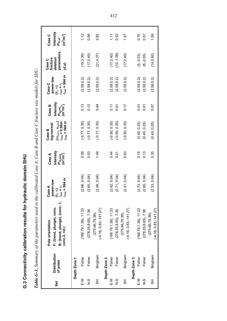
412
G.3
Co
nn
ecti
vity
cal
ibra
tio
n r
esu
lts
for
hyd
rau
lic d
om
ain
SH
U
Tab
le G
-3. S
umm
ary
of th
e pa
ram
eter
s us
ed in
the
cali
brat
ed C
ase
A, C
ase
B a
nd C
ase
C fr
actu
re s
ize
mod
els
for
SHU
.
Set
D
istr
ibu
tio
n
of
po
les
Po
le o
rien
tati
on
F:
(tre
nd
, plu
ng
e),
con
c.
B:
(tre
nd
, p
lun
ge)
, (c
on
c. 1
, co
nc.
2, r
ot.
)
Cas
e A
p
ow
er-l
aw
(kr,
r 0)
r min
= r
0
r ma
x =
564
m
Cas
e A
Inte
nsi
ty
P3
2,o
pen
(m2/m
3)
Cas
e B
lo
g-n
orm
al
(mlo
g(r
), s l
og(
r))
r min
= 0
.56m
r m
ax =
564
m
Cas
e B
Inte
nsi
ty
P3
2,P
FL
(m2/m
3)
Cas
e C
p
ow
er-l
aw
(kr,
r 0)
r min
= r
0
r ma
x =
564
m
Cas
e C
fr
actu
re
del
etio
n
par
amet
ers,
(d,a
)
Cas
e C
Inte
nsi
ty
P3
2,a
ll
(m2/m
3)
Dep
th Z
on
e 1
E-W
F
ishe
r (1
66.7
9,1.
38),
11.
23
(2.6
6, 0
.04)
0.
59
(-0.
77, 0
.35)
0.
13
(2.5
9,0.
2)
(19,
3.39
) 1.
12
N-S
F
ishe
r (2
78.2
5,8.
65),
7.3
6
(2.6
5, 0
.04)
0.
53
(-0.
77, 0
.35)
0.
12
(2.5
9,0.
2)
(17,
2.40
) 0.
99
SH
B
ing
ham
(2
75.6
6,79
.36)
,
(-4.
16,-
3.83
,-1
41.2
7)
(2.4
8, 0
.04)
1.
49
(-0.
77, 0
.35)
0.
49
(2.5
9,0.
2)
(21,
4.37
) 2.
82
Dep
th Z
on
e 2
E-W
F
ishe
r (1
66.7
9,1.
38),
11.
23
(2.4
2, 0
.04)
0.
44
(-0.
50, 0
.35)
0.
11
(2.5
9,0.
2)
(17,
2.40
) 1.
11
N-S
F
ishe
r (2
78.2
5,8.
65),
7.3
6
(2.7
1, 0
.04)
0.
21
(-0.
50,
0.35
) 0.
01
(2.5
9,0.
2)
(10,
-1.0
6)
0.52
SH
B
ing
ham
(2
75.6
6,79
.36)
,
(-4.
16,-
3.83
,-1
41.2
7)
(2.4
1, 0
.04)
0.
63
(-0.
50, 0
.35)
0.
17
(2.5
9,0.
2)
(17,
2.40
) 1.
57
Dep
th Z
on
e 3
E-W
F
ishe
r (1
66.7
9,1.
38),
11.
23
(2.7
3, 0
.04)
0.
15
(0.4
5, 0
.25)
0.
01
(2.5
9,0.
2)
(5,-
3.53
) 0.
70
N-S
F
ishe
r (2
78.2
5,8.
65),
7.3
6
(2.6
5, 0
.04)
0.
13
(0.4
5, 0
.25)
0.
01
(2.5
9,0.
2)
(8,-
2.05
) 0.
57
SH
B
ing
ham
(2
75.6
6,79
.36)
,
(-4.
16,-
3.83
,-1
41.2
7)
(2.3
3, 0
.04)
0.
35
(0.4
5, 0
.25)
0.
07
(2.5
9,0.
2)
(14,
0.92
) 1.
59
412

413
SH
U -
Dep
th Z
on
e 1
0
0.1
0.2
0.3
0.4
0.5
0.6
0.7
0.8
0.9
All
E-W
N-S
SH
Set
P10, Corr (m-1
)
Mea
sure
dC
ase
AC
ase
BC
ase
C
SH
U -
Dep
th Z
on
e 2
0
0.050.
1
0.150.
2
0.250.
3
0.35
All
E-W
N-S
SH
Set
P10, Corr (m-1
)
Mea
sure
dC
ase
AC
ase
BC
ase
C
SH
U -
Dep
th Z
on
e 3
0
0.01
0.02
0.03
0.04
0.05
0.06
0.07
0.08
0.090.
1
All
E-W
N-S
SH
Set
P10, Corr (m-1
)
Mea
sure
dC
ase
AC
ase
BC
ase
C
Fig
ure
G-3
. Com
pari
son
by fr
actu
re s
ize
mod
el a
nd d
epth
zon
e of
the
gene
rate
d an
d P
10,c
orr P
FL
frac
ture
inte
nsit
ies
for
dom
ain
SHU
.
413

G.4 Fracture size distributions for hydraulic domain CHUW
Here we show the results for the fracture size distributions for the hydraulic domain CHUW.
Fracture size distributions at each depth zone for the fracture size models Case A, Case B and Case C are shown in Figures G-4, G-5 and G-6 respectively;
A comparison of the Case A, Case B and Case C size distributions is shown in Figure G-7.
414
415
Cas
eA -
CH
UW
- D
epth
Zo
ne
1
-3.5-3
-2.5-2
-1.5-1
-0.50
0.5
-1-0
.50
0.5
11.
52
2.5
3
Lo
g (
fra
ctu
re r
adiu
s )
Log ( fracture intensity )
P1
0cor
r -
gene
rate
dP
10c
orr
- co
nnec
ted
P32
spe
cifie
dG
eo-D
FN
Cas
eA -
CH
UW
- D
epth
Zo
ne
2
-3.5-3
-2.5-2
-1.5-1
-0.50
0.5
-1-0
.50
0.5
11.
52
2.5
3
Lo
g (
fra
ctu
re r
adiu
s )
Log ( fracture intensity )
P10
corr
- g
ene
rate
dP
10c
orr
- co
nnec
ted
P3
2 sp
ecifi
ed
Geo
-DF
N
Cas
eA -
CH
UW
- D
epth
Zo
ne
3
-3.5-3
-2.5-2
-1.5-1
-0.50
0.5
-1-0
.50
0.5
11.
52
2.5
3
Lo
g (
fra
ctu
re r
adiu
s )
Log ( fracture intensity )
P1
0cor
r -
gene
rate
dP
10c
orr
- co
nnec
ted
P32
spe
cifie
dG
eo-D
FN
Cas
eA -
CH
UW
- D
epth
Zo
ne
4
-3.5-3
-2.5-2
-1.5-1
-0.50
0.5
-1-0
.50
0.5
11.
52
2.5
3
Lo
g (
fra
ctu
re r
adiu
s )
Log ( fracture intensity )
P1
0cor
r -
gene
rate
dP
10c
orr
- co
nnec
ted
P32
spe
cifie
dG
eo-D
FN
Fig
ure
G-4
. F
ract
ure
size
dis
trib
utio
ns s
how
n as
the
cum
ulat
ive
inte
nsit
y w
ithi
n a
bin
size
of
0.25
in
Log
10 (
r) f
or t
he C
ase
A s
ize
dist
ribu
tion
mod
el b
y de
pth
zone
for
CH
UW
.
415
416
Cas
eB -
CH
UW
- D
epth
Zo
ne
1
-3.5-3
-2.5-2
-1.5-1
-0.50
0.5
-1-0
.50
0.5
11.
52
2.5
3
Lo
g (
fra
ctu
re r
adiu
s )
Log ( fracture intensity )
P1
0cor
r -
gene
rate
dP
10c
orr
- co
nnec
ted
P32
spe
cifie
dG
eo-D
FN
Cas
eB -
CH
UW
- D
epth
Zo
ne
2
-3.5-3
-2.5-2
-1.5-1
-0.50
0.5
-1-0
.50
0.5
11.
52
2.5
3
Lo
g (
fra
ctu
re r
adiu
s )
Log ( fracture intensity )
P1
0cor
r -
gene
rate
dP
10c
orr
- co
nnec
ted
P32
spe
cifie
dG
eo-D
FN
C
aseB
- C
HU
W -
Dep
th Z
on
e 3
-3.5-3
-2.5-2
-1.5-1
-0.50
0.5
-1-0
.50
0.5
11.
52
2.5
3
Lo
g (
fra
ctu
re r
adiu
s )
Log ( fracture intensity )
P1
0cor
r -
gene
rate
dP
10c
orr
- co
nnec
ted
P32
spe
cifie
dG
eo-D
FN
Cas
eB -
CH
UW
- D
epth
Zo
ne
4
-3.5-3
-2.5-2
-1.5-1
-0.50
0.5
-1-0
.50
0.5
11.
52
2.5
3
Lo
g (
fra
ctu
re r
adiu
s )
Log ( fracture intensity )
P1
0cor
r -
gene
rate
dP
10c
orr
- co
nnec
ted
P32
spe
cifie
dG
eo-D
FN
Fig
ure
G-5
. F
ract
ure
size
dis
trib
utio
ns s
how
n as
the
cum
ulat
ive
inte
nsit
y w
ithi
n a
bin
size
of
0.25
in
Log
10 (
r) f
or t
he C
ase
B s
ize
dist
ribu
tion
mod
el b
y de
pth
zone
for
CH
UW
.
416
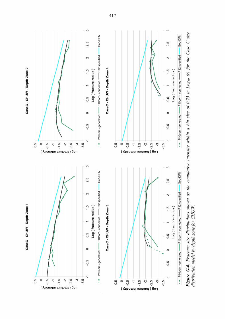
417
.
Cas
eC -
CH
UW
- D
epth
Zo
ne
1
-3.5-3
-2.5-2
-1.5-1
-0.50
0.5
-1-0
.50
0.5
11.
52
2.5
3
Lo
g (
fra
ctu
re r
adiu
s )
Log ( fracture intensity )
P1
0cor
r -
gene
rate
dP
10c
orr
- co
nnec
ted
P32
spe
cifie
dG
eo-D
FN
Cas
eC -
CH
UW
- D
epth
Zo
ne
2
-3.5-3
-2.5-2
-1.5-1
-0.50
0.5
-1-0
.50
0.5
11.
52
2.5
3
Lo
g (
fra
ctu
re r
adiu
s )
Log ( fracture intensity )
P1
0cor
r -
gene
rate
dP
10c
orr
- co
nnec
ted
P32
spe
cifie
dG
eo-D
FN
C
aseC
- C
HU
W -
Dep
th Z
on
e 3
-3.5-3
-2.5-2
-1.5-1
-0.50
0.5
-1-0
.50
0.5
11.
52
2.5
3
Lo
g (
fra
ctu
re r
adiu
s )
Log ( fracture intensity )
P1
0cor
r -
gene
rate
dP
10c
orr
- co
nnec
ted
P32
spe
cifie
dG
eo-D
FN
Cas
eC -
CH
UW
- D
epth
Zo
ne
4
-3.5-3
-2.5-2
-1.5-1
-0.50
0.5
-1-0
.50
0.5
11.
52
2.5
3
Lo
g (
fra
ctu
re r
adiu
s )
Log ( fracture intensity )
P1
0cor
r -
gene
rate
dP
10c
orr
- co
nnec
ted
P32
spe
cifie
dG
eo-D
FN
Fig
ure
G-6
. F
ract
ure
size
dis
trib
utio
ns s
how
n as
the
cum
ulat
ive
inte
nsit
y w
ithi
n a
bin
size
of
0.25
in
Log
10 (
r) f
or t
he C
ase
C s
ize
dist
ribu
tion
mod
el b
y de
pth
zone
for
CH
UW
.
417

418
All
Cas
es -
CH
UW
- D
epth
Zo
ne
1
-3.5-3
-2.5-2
-1.5-1
-0.50
0.5
-1-0
.50
0.5
11.
52
2.5
3
Lo
g (
fra
ctu
re r
adiu
s )
Log ( fracture intensity )
Ca
se A
P10
corr
- c
onn
ect
ed
Cas
e B
P10
corr
- c
onn
ecte
dC
ase
C P
10co
rr -
con
nect
edG
eo-
DF
N
All
Cas
es -
CH
UW
- D
epth
Zo
ne
2
-3.5-3
-2.5-2
-1.5-1
-0.50
0.5
-1-0
.50
0.5
11.
52
2.5
3
Lo
g (
fra
ctu
re r
adiu
s )
Log ( fracture intensity )
Ca
se A
P10
corr
- c
onn
ect
ed
Cas
e B
P10
corr
- c
onn
ecte
dC
ase
C P
10co
rr -
con
nect
edG
eo-
DF
N
All
Cas
es -
CH
UW
- D
epth
Zo
ne
3
-3.5-3
-2.5-2
-1.5-1
-0.50
0.5
-1-0
.50
0.5
11.
52
2.5
3
Lo
g (
fra
ctu
re r
adiu
s )
Log ( fracture intensity )
Ca
se A
P10
corr
- c
onn
ect
ed
Cas
e B
P10
corr
- c
onn
ecte
dC
ase
C P
10co
rr -
con
nect
edG
eo-
DF
N
All
Cas
es -
CH
UW
- D
epth
Zo
ne
4
-3.5-3
-2.5-2
-1.5-1
-0.50
0.5
-1-0
.50
0.5
11.
52
2.5
3
Lo
g (
fra
ctu
re r
adiu
s )
Log ( fracture intensity )
Ca
se A
P10
corr
- c
onn
ect
ed
Cas
e B
P10
corr
- c
onn
ecte
dC
ase
C P
10co
rr -
con
nect
edG
eo-
DF
N
Fig
ure
G-7
. F
ract
ure
size
dis
trib
utio
ns o
f co
nnec
ted
frac
ture
s sh
own
as t
he c
umul
ativ
e in
tens
ity
wit
hin
a bi
n si
ze o
f 0.
25 i
n L
og10
(r)
for
C
ases
A, B
and
C b
y de
pth
zone
for
CH
UW
.
418

419
G.5 Fracture size distributions for hydraulic domain CHUE
Here we show the results for the fracture size distributions for the hydraulic domains CHUE
Fracture size distributions at each depth zone for the fracture size models Case A, Case B and Case C are shown in Figures G-8, G-9 and G-10, respectively;
A comparison of the Case A, Case B and Case C size distributions is shown in Figure G-11.
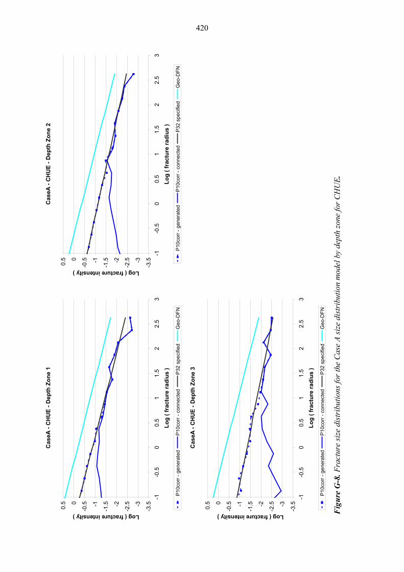
420
Cas
eA -
CH
UE
- D
epth
Zo
ne
1
-3.5-3
-2.5-2
-1.5-1
-0.50
0.5
-1-0
.50
0.5
11.
52
2.5
3
Lo
g (
fra
ctu
re r
adiu
s )
Log ( fracture intensity )
P1
0cor
r -
gene
rate
dP
10c
orr
- co
nnec
ted
P32
spe
cifie
dG
eo-D
FN
Cas
eA -
CH
UE
- D
epth
Zo
ne
2
-3.5-3
-2.5-2
-1.5-1
-0.50
0.5
-1-0
.50
0.5
11.
52
2.5
3
Lo
g (
fra
ctu
re r
adiu
s )
Log ( fracture intensity )
P10
corr
- g
ene
rate
dP
10c
orr
- co
nnec
ted
P3
2 sp
ecifi
ed
Geo
-DF
N
Cas
eA -
CH
UE
- D
epth
Zo
ne
3
-3.5-3
-2.5-2
-1.5-1
-0.50
0.5
-1-0
.50
0.5
11.
52
2.5
3
Lo
g (
fra
ctu
re r
adiu
s )
Log ( fracture intensity )
P1
0cor
r -
gene
rate
dP
10c
orr
- co
nnec
ted
P32
spe
cifie
dG
eo-D
FN
Fig
ure
G-8
. Fra
ctur
e si
ze d
istr
ibut
ions
for
the
Cas
e A
siz
e di
stri
buti
on m
odel
by
dept
h zo
ne fo
r C
HU
E.
420
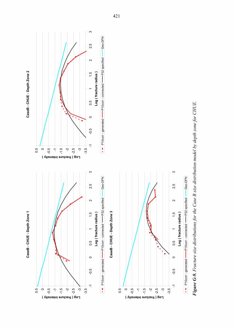
421
Cas
eB -
CH
UE
- D
epth
Zo
ne
1
-3.5-3
-2.5-2
-1.5-1
-0.50
0.5
-1-0
.50
0.5
11.
52
2.5
3
Lo
g (
fra
ctu
re r
adiu
s )
Log ( fracture intensity )
P1
0cor
r -
gene
rate
dP
10c
orr
- co
nnec
ted
P32
spe
cifie
dG
eo-D
FN
Cas
eB -
CH
UE
- D
epth
Zo
ne
2
-3.5-3
-2.5-2
-1.5-1
-0.50
0.5
-1-0
.50
0.5
11.
52
2.5
3
Lo
g (
fra
ctu
re r
adiu
s )
Log ( fracture intensity )
P1
0cor
r -
gene
rate
dP
10c
orr
- co
nnec
ted
P32
spe
cifie
dG
eo-D
FN
C
aseB
- C
HU
E -
Dep
th Z
on
e 3
-3.5-3
-2.5-2
-1.5-1
-0.50
0.5
-1-0
.50
0.5
11.
52
2.5
3
Lo
g (
fra
ctu
re r
adiu
s )
Log ( fracture intensity )
P1
0cor
r -
gene
rate
dP
10c
orr
- co
nnec
ted
P32
spe
cifie
dG
eo-D
FN
Fig
ure
G-9
. Fra
ctur
e si
ze d
istr
ibut
ions
for
the
Cas
e B
siz
e di
stri
buti
on m
odel
by
dept
h zo
ne fo
r C
HU
E.
421
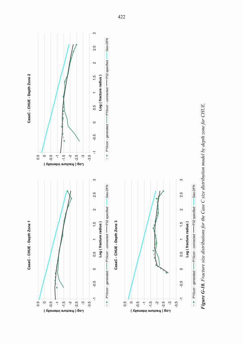
422
Cas
eC -
CH
UE
- D
epth
Zo
ne
1
-3.5-3
-2.5-2
-1.5-1
-0.50
0.5
-1-0
.50
0.5
11.
52
2.5
3
Lo
g (
fra
ctu
re r
adiu
s )
Log ( fracture intensity )
P1
0cor
r -
gene
rate
dP
10c
orr
- co
nnec
ted
P32
spe
cifie
dG
eo-D
FN
Cas
eC -
CH
UE
- D
epth
Zo
ne
2
-3.5-3
-2.5-2
-1.5-1
-0.50
0.5
-1-0
.50
0.5
11.
52
2.5
3
Lo
g (
fra
ctu
re r
adiu
s )
Log ( fracture intensity )
P1
0cor
r -
gene
rate
dP
10c
orr
- co
nnec
ted
P32
spe
cifie
dG
eo-D
FN
C
aseC
- C
HU
E -
Dep
th Z
on
e 3
-3.5-3
-2.5-2
-1.5-1
-0.50
0.5
-1-0
.50
0.5
11.
52
2.5
3
Lo
g (
fra
ctu
re r
adiu
s )
Log ( fracture intensity )
P1
0cor
r -
gene
rate
dP
10c
orr
- co
nnec
ted
P32
spe
cifie
dG
eo-D
FN
Fig
ure
G-1
0. F
ract
ure
size
dis
trib
utio
ns fo
r th
e C
ase
C s
ize
dist
ribu
tion
mod
el b
y de
pth
zone
for
CH
UE
.
422
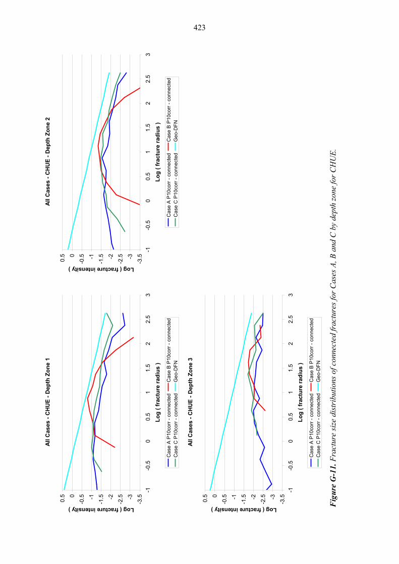
423
All
Cas
es -
CH
UE
- D
epth
Zo
ne
1
-3.5-3
-2.5-2
-1.5-1
-0.50
0.5
-1-0
.50
0.5
11.
52
2.5
3
Lo
g (
fra
ctu
re r
adiu
s )
Log ( fracture intensity )
Ca
se A
P10
corr
- c
onn
ect
ed
Cas
e B
P10
corr
- c
onn
ecte
dC
ase
C P
10co
rr -
con
nect
edG
eo-
DF
N
All
Cas
es -
CH
UE
- D
epth
Zo
ne
2
-3.5-3
-2.5-2
-1.5-1
-0.50
0.5
-1-0
.50
0.5
11.
52
2.5
3
Lo
g (
fra
ctu
re r
adiu
s )
Log ( fracture intensity )
Ca
se A
P10
corr
- c
onn
ect
ed
Cas
e B
P10
corr
- c
onn
ecte
dC
ase
C P
10co
rr -
con
nect
edG
eo-
DF
N
All
Cas
es -
CH
UE
- D
epth
Zo
ne
3
-3.5-3
-2.5-2
-1.5-1
-0.50
0.5
-1-0
.50
0.5
11.
52
2.5
3
Lo
g (
fra
ctu
re r
adiu
s )
Log ( fracture intensity )
Ca
se A
P10
corr
- c
onn
ect
ed
Cas
e B
P10
corr
- c
onn
ecte
dC
ase
C P
10co
rr -
con
nect
edG
eo-
DF
N
Fig
ure
G-1
1. F
ract
ure
size
dis
trib
utio
ns o
f con
nect
ed fr
actu
res
for
Cas
es A
, B a
nd C
by
dept
h zo
ne fo
r C
HU
E.
423

424
G.6 Fracture size distributions for hydraulic domain SHU
Here we show the results for the fracture size distributions for the hydraulic domain SHU
Fracture size distributions at each depth zone for the fracture size models Case A, Case B and Case C are shown in Figures G-12, G-13 and G-14, respectively;
A comparison of the Case A, Case B and Case C size distributions is shown in Figure G-15.

425
Cas
eA -
SH
U -
Dep
th Z
on
e 1
-3.5-3
-2.5-2
-1.5-1
-0.50
0.5
-1-0
.50
0.5
11.
52
2.5
3
Lo
g (
fra
ctu
re r
adiu
s )
Log ( fracture intensity )
P1
0cor
r -
gene
rate
dP
10c
orr
- co
nnec
ted
P32
spe
cifie
dG
eo-D
FN
Cas
eA -
SH
U -
Dep
th Z
on
e 2
-3.5-3
-2.5-2
-1.5-1
-0.50
0.5
-1-0
.50
0.5
11.
52
2.5
3
Lo
g (
fra
ctu
re r
adiu
s )
Log ( fracture intensity )
P10
corr
- g
ene
rate
dP
10c
orr
- co
nnec
ted
P3
2 sp
ecifi
ed
Geo
-DF
N
Cas
eA -
SH
U -
Dep
th Z
on
e 3
-3.5-3
-2.5-2
-1.5-1
-0.50
0.5
-1-0
.50
0.5
11.
52
2.5
3
Lo
g (
fra
ctu
re r
adiu
s )
Log ( fracture intensity )
P1
0cor
r -
gene
rate
dP
10c
orr
- co
nnec
ted
P32
spe
cifie
dG
eo-D
FN
Fig
ure
G-1
2. F
ract
ure
size
dis
trib
utio
ns fo
r th
e C
ase
A s
ize
dist
ribu
tion
mod
el b
y de
pth
zone
for
SHU
.
425
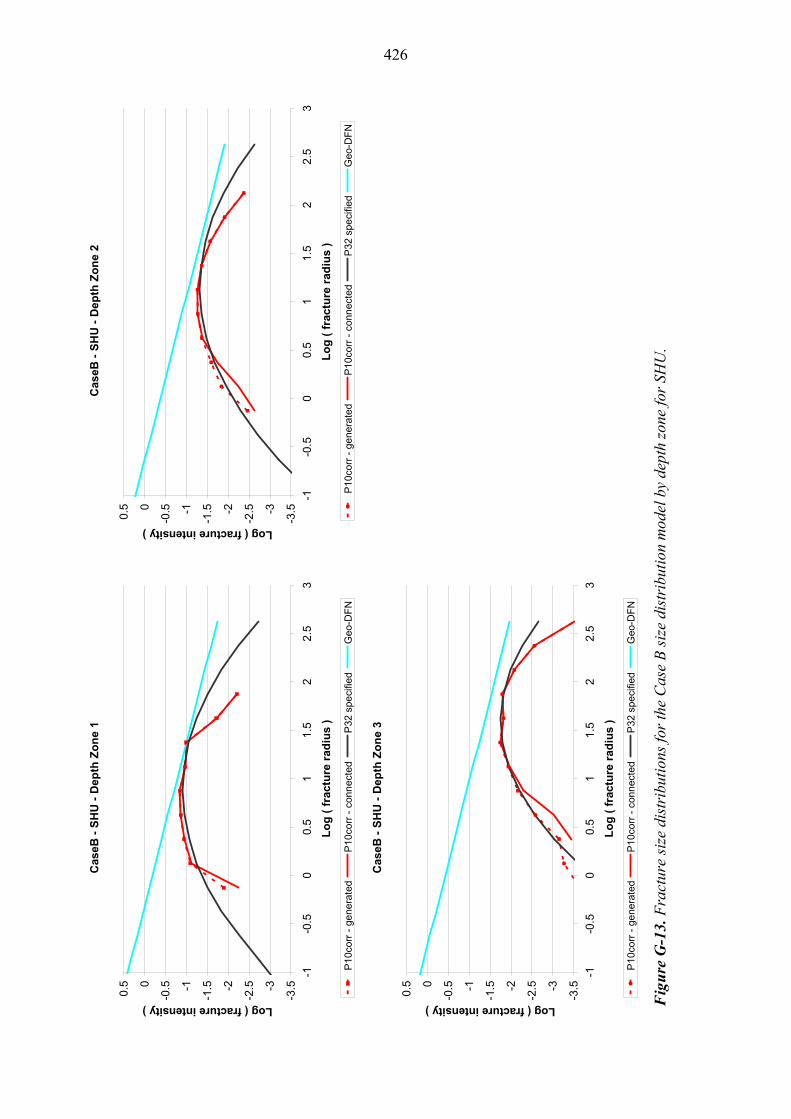
426
Cas
eB -
SH
U -
Dep
th Z
on
e 1
-3.5-3
-2.5-2
-1.5-1
-0.50
0.5
-1-0
.50
0.5
11.
52
2.5
3
Lo
g (
fra
ctu
re r
adiu
s )
Log ( fracture intensity )
P1
0cor
r -
gene
rate
dP
10c
orr
- co
nnec
ted
P32
spe
cifie
dG
eo-D
FN
Cas
eB -
SH
U -
Dep
th Z
on
e 2
-3.5-3
-2.5-2
-1.5-1
-0.50
0.5
-1-0
.50
0.5
11.
52
2.5
3
Lo
g (
fra
ctu
re r
adiu
s )
Log ( fracture intensity )
P1
0cor
r -
gene
rate
dP
10c
orr
- co
nnec
ted
P32
spe
cifie
dG
eo-D
FN
C
aseB
- S
HU
- D
epth
Zo
ne
3
-3.5-3
-2.5-2
-1.5-1
-0.50
0.5
-1-0
.50
0.5
11.
52
2.5
3
Lo
g (
fra
ctu
re r
adiu
s )
Log ( fracture intensity )
P1
0cor
r -
gene
rate
dP
10c
orr
- co
nnec
ted
P32
spe
cifie
dG
eo-D
FN
Fig
ure
G-1
3. F
ract
ure
size
dis
trib
utio
ns fo
r th
e C
ase
B s
ize
dist
ribu
tion
mod
el b
y de
pth
zone
for
SHU
.
426
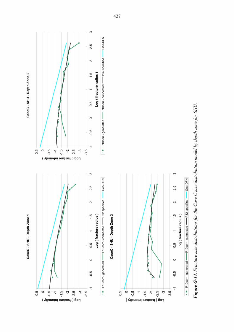
427
Cas
eC -
SH
U -
Dep
th Z
on
e 1
-3.5-3
-2.5-2
-1.5-1
-0.50
0.5
-1-0
.50
0.5
11.
52
2.5
3
Lo
g (
fra
ctu
re r
adiu
s )
Log ( fracture intensity )
P1
0cor
r -
gene
rate
dP
10c
orr
- co
nnec
ted
P32
spe
cifie
dG
eo-D
FN
Cas
eC -
SH
U -
Dep
th Z
on
e 2
-3.5-3
-2.5-2
-1.5-1
-0.50
0.5
-1-0
.50
0.5
11.
52
2.5
3
Lo
g (
fra
ctu
re r
adiu
s )
Log ( fracture intensity )
P1
0cor
r -
gene
rate
dP
10c
orr
- co
nnec
ted
P32
spe
cifie
dG
eo-D
FN
C
aseC
- S
HU
- D
epth
Zo
ne
3
-3.5-3
-2.5-2
-1.5-1
-0.50
0.5
-1-0
.50
0.5
11.
52
2.5
3
Lo
g (
fra
ctu
re r
adiu
s )
Log ( fracture intensity )
P1
0cor
r -
gene
rate
dP
10c
orr
- co
nnec
ted
P32
spe
cifie
dG
eo-D
FN
Fig
ure
G-1
4. F
ract
ure
size
dis
trib
utio
ns fo
r th
e C
ase
C s
ize
dist
ribu
tion
mod
el b
y de
pth
zone
for
SHU
.
427

All
Cas
es -
SH
U -
Dep
th Z
on
e 1
-3.5-3
-2.5-2
-1.5-1
-0.50
0.5
-1-0
.50
0.5
11.
52
2.5
3
Lo
g (
fra
ctu
re r
adiu
s )
Log ( fracture intensity )
Ca
se A
P10
corr
- c
onn
ect
ed
Cas
e B
P10
corr
- c
onn
ecte
dC
ase
C P
10co
rr -
con
nect
edG
eo-
DF
N
All
Cas
es -
SH
U -
Dep
th Z
on
e 2
-3.5-3
-2.5-2
-1.5-1
-0.50
0.5
-1-0
.50
0.5
11.
52
2.5
3
Lo
g (
fra
ctu
re r
adiu
s )
Log ( fracture intensity )
Ca
se A
P10
corr
- c
onn
ect
ed
Cas
e B
P10
corr
- c
onn
ecte
dC
ase
C P
10co
rr -
con
nect
edG
eo-
DF
N
All
Cas
es -
SH
U -
Dep
th Z
on
e 3
-3.5-3
-2.5-2
-1.5-1
-0.50
0.5
-1-0
.50
0.5
11.
52
2.5
3
Lo
g (
fra
ctu
re r
adiu
s )
Log ( fracture intensity )
Ca
se A
P10
corr
- c
onn
ect
ed
Cas
e B
P10
corr
- c
onn
ecte
dC
ase
C P
10co
rr -
con
nect
edG
eo-
DF
N
Fig
ure
G-1
5. F
ract
ure
size
dis
trib
utio
ns o
f con
nect
ed fr
actu
res
for
Cas
es A
, B a
nd C
by
dept
h zo
ne fo
r SH
U.
428
429
APPENDIX H: FLOW CALIBRATION RESULTS
This Appendix presents the results from the flow calibration for the hydraulic domains CHUW, CHUE and SHU. (Results for the hydraulic domain NHU are shown in the main text in Chapter 5).
For hydraulic domain CHUW:
o The quality of the match of the Hydro-DFN models using semi-correlated transmissivities, to the observed distributions of PFL flows are presented in Figure H-1 through Figure H-10.
o A summary of the calibrated transmissivity parameters for the flow models in hydraulic domain CHUW are shown in Table H-2 through Table H-4.
For hydraulic domain CHUE:
o The quality of the match of the Hydro-DFN models using semi-correlated transmissivities, to the observed distributions of PFL flows are presented in Figure H-11 through Figure H-20.
o A summary of the calibrated transmissivity parameters for the flow models in hydraulic domain CHUW are shown in Table H-6 through Table H-8.
For hydraulic domain SHU:
o The quality of the match of the Hydro-DFN models using semi-correlated transmissivities, to the observed distributions of PFL flows are presented in Figure H-21 through Figure H-30.
o A summary of the calibrated transmissivity parameters for the flow models in hydraulic domain SHU are shown in Table H-10 through Table H-12.
For Case A, three different correlations between fracture transmissivity and fracture size are considered: Correlated, Semi-Correlated and Uncorrelated. For Cases B and C, only the semi-correlated model is used. (Note that for hydraulic domains CHUE and SHU, due to the lack of data in Depth Zone 4 for these two hydraulic domains, no flow calibration results are presented. For these two domains, transmissivity parameters for CHUW have been assumed).
H.1 Flow calibration for hydraulic domain CHUW
The results for the flow calibrations of hydraulic domain CHUW are presented below.
Figure H-1, Figure H-5 and Figure H-8 illustrate histograms of the distribution of specific capacity, Q/s, for a bin size of half an order of magnitude compared with equivalent PFL data for each of the semi-correlated Case A, B and C fracture size distributions respectively. Corresponding correlation coefficients
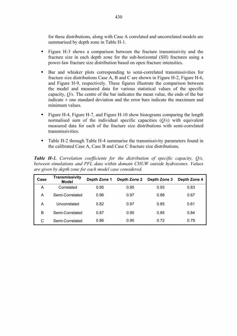
430
for these distributions, along with Case A correlated and uncorrelated models are summarised by depth zone in Table H-1.
Figure H-3 shows a comparison between the fracture transmissivity and the fracture size in each depth zone for the sub-horizontal (SH) fractures using a power-law fracture size distribution based on open fracture intensities.
Bar and whisker plots corresponding to semi-correlated transmissivities for fracture size distributions Case A, B and C are shown in Figure H-2, Figure H-6, and Figure H-9, respectively. These figures illustrate the comparison between the model and measured data for various statistical values of the specific capacity, Q/s. The centre of the bar indicates the mean value, the ends of the bar indicate ± one standard deviation and the error bars indicate the maximum and minimum values.
Figure H-4, Figure H-7, and Figure H-10 show histograms comparing the length normalised sum of the individual specific capacities (Q/s) with equivalent measured data for each of the fracture size distributions with semi-correlated transmissivities.
Table H-2 through Table H-4 summarise the transmissivity parameters found in the calibrated Case A, Case B and Case C fracture size distributions.
Table H-1. Correlation coefficients for the distribution of specific capacity, Q/s, between simulations and PFL data within domain CHUW outside hydrozones. Values are given by depth zone for each model case considered.
Case Transmissivity
Model Depth Zone 1 Depth Zone 2 Depth Zone 3 Depth Zone 4
A Correlated 0.95 0.95 0.93 0.83
A Semi-Correlated 0.96 0.97 0.88 0.67
A Uncorrelated 0.82 0.97 0.85 0.61
B Semi-Correlated 0.87 0.95 0.85 0.84
C Semi-Correlated 0.86 0.95 0.72 0.79
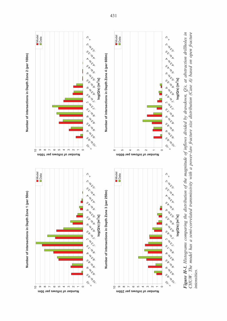
Nu
mb
er
of
inte
rsec
tio
ns
in D
epth
Zo
ne
1 (
per
50m
)
012345678910
< -1
0 -10
to -9
.5 -9.5
to -9 -9
to -8
.5 -8.5
to -8 -8
to -7
.5 -7.5
to -7 -7
to -6
.5 -6.5
to -6 -6
to -5
.5 -5.5
to -5 -5
to -4
.5 -4.5
to -4 -4
to -3
.5 -3.5
to -3
> -3
log
(Q/s
) [m
2 /s]
Number of inflows per 50m
Mod
elD
ata
Nu
mb
er o
f in
ters
ecti
on
s in
Dep
th Z
on
e 2
(per
100
m)
012345678910
< -1
0 -10
to -9
.5 -9.5
to -9 -9
to -8
.5 -8.5
to -8 -8
to -7
.5 -7.5
to -7 -7
to -6
.5 -6.5
to -6 -6
to -5
.5 -5.5
to -5 -5
to -4
.5 -4.5
to -4 -4
to -3
.5 -3.5
to -3
> -3
log
(Q/s
) [m
2 /s]
Number of inflows per 100m
Mod
elD
ata
Nu
mb
er o
f in
ters
ecti
on
s in
Dep
th Z
on
e 3
(per
250
m)
012345678910
< -1
0 -10
to -9
.5 -9.5
to -9 -9
to -8
.5 -8.5
to -8 -8
to -7
.5 -7.5
to -7 -7
to -6
.5 -6.5
to -6 -6
to -5
.5 -5.5
to -5 -5
to -4
.5 -4.5
to -4 -4
to -3
.5 -3.5
to -3
> -3
log
(Q/s
) [m
2 /s]
Number of inflows per 250m
Mod
elD
ata
Nu
mb
er o
f in
ters
ecti
on
s in
Dep
th Z
on
e 4
(per
600
m)
0123456
< -1
0 -10
to -9
.5 -9.5
to -9 -9
to -8
.5 -8.5
to -8 -8
to -7
.5 -7.5
to -7 -7
to -6
.5 -6.5
to -6 -6
to -5
.5 -5.5
to -5 -5
to -4
.5 -4.5
to -4 -4
to -3
.5 -3.5
to -3
> -3
log
(Q/s
) [m
2 /s]
Number of inflows per 600m
Mod
elD
ata
Fig
ure
H-1
. His
togr
ams
com
pari
ng th
e di
stri
butio
n of
the
mag
nitu
de o
f inf
low
s di
vide
d by
dra
wdo
wn,
Q/s
, at a
bstr
actio
n dr
illho
les
in
CH
UW
. Th
e m
odel
has
a s
emi-c
orre
late
d tr
ansm
issi
vity
with
a p
ower
-law
fra
ctur
e si
ze d
istr
ibut
ion
(Cas
e A)
bas
ed o
n op
en f
ract
ure
inte
nsiti
es.
431
432
Infl
ow
s in
Dep
th Z
on
e 1
(per
50m
)
-10.
0-9
.0-8
.0-7
.0-6
.0-5
.0-4
.0-3
.0-2
.0-1
.00.
0
PF
L E
-W
Mod
el E
-W
PF
L N
-S
Mod
el N
-S
PF
L S
H
Mod
el S
H
Fracture set
log
(Q
/s)
[m2/s
]
8.0
4.3
5.4
8.7
28.9
26.8
Infl
ow
s in
Dep
th Z
on
e 2
(p
er 1
00m
)
-10.
0-9
.0-8
.0-7
.0-6
.0-5
.0-4
.0-3
.0-2
.0-1
.00.
0
PF
L E
-W
Mod
el E
-W
PF
L N
-S
Mod
el N
-S
PF
L S
H
Mod
el S
H
Fracture set
log
(Q
/s)
[m2/s
]
4.7
3.1
3.7
5.9
18.0
18.6
Infl
ow
s in
Dep
th Z
on
e 3
(per
250
m)
-10.
0-9
.0-8
.0-7
.0-6
.0-5
.0-4
.0-3
.0-2
.0-1
.00.
0
PF
L E
-W
Mod
el E
-W
PF
L N
-S
Mod
el N
-S
PF
L S
H
Mod
el S
H
Fracture set
log
(Q
/s)
[m2/s
]
1.7
2.6
3.5
2.0
15.8
15.3
Infl
ow
s in
Dep
th Z
on
e 4
(per
600
m)
-10.
0-9
.0-8
.0-7
.0-6
.0-5
.0-4
.0-3
.0-2
.0-1
.00.
0
PF
L E
-W
Mod
el E
-W
PF
L N
-S
Mod
el N
-S
PF
L S
H
Mod
el S
H
Fracture set
log
(Q
/s)
[m2/s
]
1.0
1.4
1.6
0.8
4.9
4.4
Fig
ure
H-2
. Bar
and
whi
sker
plo
ts c
ompa
ring
sta
tist
ics
for
each
frac
ture
set
for
the
indi
vidu
al in
flow
s, Q
/s, f
or th
e P
FL
dat
a fr
om d
rill
hole
se
ctio
ns w
ithi
n C
HU
W a
gain
st s
tati
stic
s fo
r an
ens
embl
e of
40
real
isat
ions
(10
rea
lisa
tion
s pe
r dr
illh
ole)
of
the
Hyd
ro-D
FN
mod
el
(Cas
e A
).
432

433
De
pth
Zo
ne
1: S
ub
-Ho
rizo
nta
l
-11.
00
-10.
00
-9.0
0
-8.0
0
-7.0
0
-6.0
0
-5.0
0
-4.0
0
-3.0
0
-2-1
01
23
Lo
g1
0(r
) (m
)
Log10(T) (m2/s)
SC
SC
sp
read
C UC
UC
spr
ead
De
pth
Zo
ne
2:
Su
b-H
ori
zon
tal
-11.
00
-10.
00
-9.0
0
-8.0
0
-7.0
0
-6.0
0
-5.0
0
-4.0
0
-3.0
0
-2-1
01
23
Lo
g1
0(r
) (m
)
Log10(T) (m2/s)
SC
SC
spr
ea
dC U
CU
C s
pre
ad
De
pth
Zo
ne
3: S
ub
-Ho
rizo
nta
l
-11.
00
-10.
00
-9.0
0
-8.0
0
-7.0
0
-6.0
0
-5.0
0
-4.0
0
-3.0
0
-2-1
01
23
Lo
g1
0(r
) (m
)
Log10(T) (m2/s)
SC
SC
spr
ead
C UC
UC
spr
ead
De
pth
Zo
ne
4:
Su
b-H
ori
zon
tal
-11.
00
-10.
00
-9.0
0
-8.0
0
-7.0
0
-6.0
0
-5.0
0
-4.0
0
-3.0
0
-2-1
01
23
Lo
g1
0(r
) (m
)
Log10(T) (m2/s)
SC
SC
spr
ea
dC U
CU
C s
pre
ad
Fig
ure
H-3
. Com
pari
son
of th
e re
lati
onsh
ip b
etw
een
frac
ture
tran
smis
sivi
ty a
nd fr
actu
re s
ize
in e
ach
dept
h zo
ne fo
r C
HU
W. T
he p
lots
are
fo
r th
e ca
libr
ated
mod
el o
f su
b-ho
rizo
ntal
fra
ctur
es,
usin
g a
pow
er-l
aw f
ract
ure
size
dis
trib
utio
n (C
ase
A)
base
d on
ope
n fr
actu
re
inte
nsit
ies.
The
plo
ts s
how
the
cen
tral
tre
nd f
or e
ach
rela
tion
ship
tog
ethe
r w
ith
line
s at
1 s
tand
ard
devi
atio
n ab
ove
and
belo
w t
he c
entr
al
tren
d.
433

434
Total normalized flow to borehole section (Terzaghi corrected)
-4.8
-5.6 -5
.4
-6.8
-4.8
-5.7 -5
.4
-6.7
-8.5
-8.0
-7.5
-7.0
-6.5
-6.0
-5.5
-5.0
-4.5
-4.0
-3.5
DZ1 DZ2 DZ3 DZ4
Depth Zone
Lo
g [
Flo
w (
Q/s
)] [
m2 /s
]
Model
Data
Figure H-4. Comparison of the Terzaghi weighted sum of individual specific capacities, Q/s, for the PFL data from drillhole sections within CHUW normalised to the nominal thicknesses of each depth zone against statistics for an ensemble over 10 realisations of 4 individual drillholes in the Hydro-DFN model. The model has a semi-correlated transmissivity with a power-law fracture size distribution (Case A) based on open fracture intensities. For the data, statistics are taken over the identified flowing fractures within each set. For the model, statistics are generated over 40 realisations. The total flows are normalised to the following lengths: Depth Zone 1 is 50 m, Depth Zone 2 is 100 m, Depth Zone 3 is 250 m, and Depth Zone 4 is 600 m.
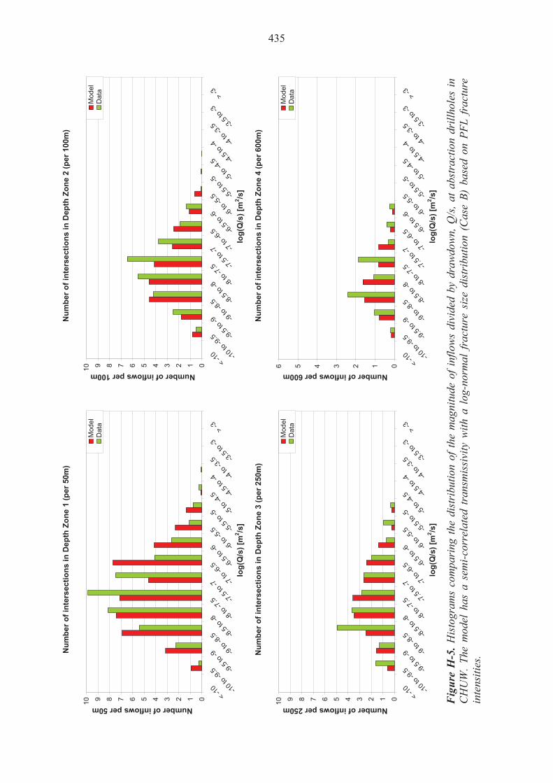
Nu
mb
er
of
inte
rsec
tio
ns
in D
epth
Zo
ne
1 (
per
50m
)
012345678910
< -1
0 -10
to -9
.5 -9.5
to -9 -9
to -8
.5 -8.5
to -8 -8
to -7
.5 -7.5
to -7 -7
to -6
.5 -6.5
to -6 -6
to -5
.5 -5.5
to -5 -5
to -4
.5 -4.5
to -4 -4
to -3
.5 -3.5
to -3
> -3
log
(Q/s
) [m
2 /s]
Number of inflows per 50m
Mod
elD
ata
Nu
mb
er o
f in
ters
ecti
on
s in
Dep
th Z
on
e 2
(per
100
m)
012345678910
< -1
0 -10
to -9
.5 -9.5
to -9 -9
to -8
.5 -8.5
to -8 -8
to -7
.5 -7.5
to -7 -7
to -6
.5 -6.5
to -6 -6
to -5
.5 -5.5
to -5 -5
to -4
.5 -4.5
to -4 -4
to -3
.5 -3.5
to -3
> -3
log
(Q/s
) [m
2 /s]
Number of inflows per 100m
Mod
elD
ata
Nu
mb
er o
f in
ters
ecti
on
s in
Dep
th Z
on
e 3
(per
250
m)
012345678910
< -1
0 -10
to -9
.5 -9.5
to -9 -9
to -8
.5 -8.5
to -8 -8
to -7
.5 -7.5
to -7 -7
to -6
.5 -6.5
to -6 -6
to -5
.5 -5.5
to -5 -5
to -4
.5 -4.5
to -4 -4
to -3
.5 -3.5
to -3
> -3
log
(Q/s
) [m
2 /s]
Number of inflows per 250m
Mod
elD
ata
Nu
mb
er o
f in
ters
ecti
on
s in
Dep
th Z
on
e 4
(per
600
m)
0123456
< -1
0 -10
to -9
.5 -9.5
to -9 -9
to -8
.5 -8.5
to -8 -8
to -7
.5 -7.5
to -7 -7
to -6
.5 -6.5
to -6 -6
to -5
.5 -5.5
to -5 -5
to -4
.5 -4.5
to -4 -4
to -3
.5 -3.5
to -3
> -3
log
(Q/s
) [m
2 /s]
Number of inflows per 600m
Mod
elD
ata
Fig
ure
H-5
. His
togr
ams
com
pari
ng th
e di
stri
butio
n of
the
mag
nitu
de o
f inf
low
s di
vide
d by
dra
wdo
wn,
Q/s
, at a
bstr
actio
n dr
illho
les
in
CH
UW
. The
mod
el h
as a
sem
i-cor
rela
ted
tran
smis
sivi
ty w
ith a
log
-nor
mal
fra
ctur
e si
ze d
istr
ibut
ion
(Cas
e B)
bas
ed o
n PF
L fr
actu
re
inte
nsiti
es.
435
436
Infl
ow
s in
Dep
th Z
on
e 1
(per
50m
)
-10.
0-9
.0-8
.0-7
.0-6
.0-5
.0-4
.0-3
.0-2
.0-1
.00.
0
PF
L E
-W
Mod
el E
-W
PF
L N
-S
Mod
el N
-S
PF
L S
H
Mod
el S
H
Fracture set
log
(Q
/s)
[m2/s
]
8.0
5.4
5.4
8.7
28.9
31.7
Infl
ow
s in
Dep
th Z
on
e 2
(p
er 1
00m
)
-10.
0-9
.0-8
.0-7
.0-6
.0-5
.0-4
.0-3
.0-2
.0-1
.00.
0
PF
L E
-W
Mod
el E
-W
PF
L N
-S
Mod
el N
-S
PF
L S
H
Mod
el S
H
Fracture set
log
(Q
/s)
[m2/s
]
4.7
2.8
3.7
3.5
18.0
16.2
Infl
ow
s in
Dep
th Z
on
e 3
(per
250
m)
-10.
0-9
.0-8
.0-7
.0-6
.0-5
.0-4
.0-3
.0-2
.0-1
.00.
0
PF
L E
-W
Mod
el E
-W
PF
L N
-S
Mod
el N
-S
PF
L S
H
Mod
el S
H
Fracture set
log
(Q
/s)
[m2/s
]
1.7
3.1
3.5
1.9
15.8
13.5
Infl
ow
s in
Dep
th Z
on
e 4
(per
600
m)
-10.
0-9
.0-8
.0-7
.0-6
.0-5
.0-4
.0-3
.0-2
.0-1
.00.
0
PF
L E
-W
Mod
el E
-W
PF
L N
-S
Mod
el N
-S
PF
L S
H
Mod
el S
H
Fracture set
log
(Q
/s)
[m2/s
]
1.0
1.2
1.6
0.9
4.9
4.0
Fig
ure
H-6
. Bar
and
whi
sker
plo
ts c
ompa
ring
sta
tist
ics
for
each
frac
ture
set
for
the
indi
vidu
al in
flow
s, Q
/s, f
or th
e P
FL
dat
a fr
om d
rill
hole
se
ctio
ns w
ithi
n C
HU
W a
gain
st s
tati
stic
s fo
r an
ens
embl
e of
40
real
isat
ions
(10
rea
lisa
tion
s pe
r dr
illh
ole)
of
the
Hyd
ro-D
FN
mod
el (
Cas
e B
). T
he n
umbe
rs a
djac
ent t
o ea
ch b
ar a
re th
e Te
rzag
hi w
eigh
ted
num
bers
of s
peci
fic
capa
citi
es a
bove
1.6
10-1
0 m2 /s
.
436

437
Total normalized flow to borehole section (Terzaghi corrected)
-4.8
-5.6 -5
.5
-6.8
-4.8
-5.7 -5
.4
-6.7
-8.5
-8.0
-7.5
-7.0
-6.5
-6.0
-5.5
-5.0
-4.5
-4.0
-3.5
DZ1 DZ2 DZ3 DZ4
Depth Zone
Lo
g [
Flo
w (
Q/s
)] [
m2 /s
]
Model
Data
Figure H-7. Comparison of the Terzaghi weighted sum of individual specific capacities, Q/s, for the PFL data from drillhole sections within CHUW normalised to the nominal thicknesses of each depth zone, against statistics for an ensemble over 10 realisations of 4 individual drillholes in the Hydro-DFN model. The model has a semi-correlated transmissivity with a log-normal fracture size distribution (Case B) based on PFL fracture intensities. For the data, statistics are taken over the identified flowing fractures within each set. For the model, statistics are generated over 40 realisations. The total flows are normalised to the following lengths: Depth Zone 1 is 50m, Depth Zone 2 is 100 m, Depth Zone 3 is 250 m, and Depth Zone 4 is 600 m.
Nu
mb
er
of
inte
rsec
tio
ns
in D
epth
Zo
ne
1 (
per
50m
)
012345678910
< -1
0 -10
to -9
.5 -9.5
to -9 -9
to -8
.5 -8.5
to -8 -8
to -7
.5 -7.5
to -7 -7
to -6
.5 -6.5
to -6 -6
to -5
.5 -5.5
to -5 -5
to -4
.5 -4.5
to -4 -4
to -3
.5 -3.5
to -3
> -3
log
(Q/s
) [m
2 /s]
Number of inflows per 50mM
odel
Dat
a
Nu
mb
er o
f in
ters
ecti
on
s in
Dep
th Z
on
e 2
(per
100
m)
012345678910
< -1
0 -10
to -9
.5 -9.5
to -9 -9
to -8
.5 -8.5
to -8 -8
to -7
.5 -7.5
to -7 -7
to -6
.5 -6.5
to -6 -6
to -5
.5 -5.5
to -5 -5
to -4
.5 -4.5
to -4 -4
to -3
.5 -3.5
to -3
> -3
log
(Q/s
) [m
2 /s]
Number of inflows per 100m
Mod
elD
ata
Nu
mb
er o
f in
ters
ecti
on
s in
Dep
th Z
on
e 3
(per
250
m)
012345678910
< -1
0 -10
to -9
.5 -9.5
to -9 -9
to -8
.5 -8.5
to -8 -8
to -7
.5 -7.5
to -7 -7
to -6
.5 -6.5
to -6 -6
to -5
.5 -5.5
to -5 -5
to -4
.5 -4.5
to -4 -4
to -3
.5 -3.5
to -3
> -3
log
(Q/s
) [m
2 /s]
Number of inflows per 250m
Mod
elD
ata
Nu
mb
er o
f in
ters
ecti
on
s in
Dep
th Z
on
e 4
(per
600
m)
0123456
< -1
0 -10
to -9
.5 -9.5
to -9 -9
to -8
.5 -8.5
to -8 -8
to -7
.5 -7.5
to -7 -7
to -6
.5 -6.5
to -6 -6
to -5
.5 -5.5
to -5 -5
to -4
.5 -4.5
to -4 -4
to -3
.5 -3.5
to -3
> -3
log
(Q/s
) [m
2 /s]
Number of inflows per 600m
Mod
elD
ata
Fig
ure
H-8
. His
togr
ams
com
pari
ng th
e di
stri
butio
n of
the
mag
nitu
de o
f inf
low
s di
vide
d by
dra
wdo
wn,
Q/s
, at a
bstr
actio
n dr
illho
les
in
CH
UW
. Th
e m
odel
has
a s
emi-c
orre
late
d tr
ansm
issi
vity
with
a p
ower
-law
fra
ctur
e si
ze d
istr
ibut
ion
(Cas
e C
) ba
sed
on a
ll fr
actu
re
inte
nsiti
es.
438
439
Infl
ow
s in
Dep
th Z
on
e 1
(per
50m
)
-10.
0-9
.0-8
.0-7
.0-6
.0-5
.0-4
.0-3
.0-2
.0-1
.00.
0
PF
L E
-W
Mod
el E
-W
PF
L N
-S
Mod
el N
-S
PF
L S
H
Mod
el S
H
Fracture set
log
(Q
/s)
[m2/s
]
8.0
1.7
5.4
8.8
28.9
22.5
Infl
ow
s in
Dep
th Z
on
e 2
(p
er 1
00m
)
-10.
0-9
.0-8
.0-7
.0-6
.0-5
.0-4
.0-3
.0-2
.0-1
.00.
0
PF
L E
-W
Mod
el E
-W
PF
L N
-S
Mod
el N
-S
PF
L S
H
Mod
el S
H
Fracture set
log
(Q
/s)
[m2/s
]
4.7
3.7
3.7
5.8
18.0
16.6
Infl
ow
s in
Dep
th Z
on
e 3
(per
250
m)
-10.
0-9
.0-8
.0-7
.0-6
.0-5
.0-4
.0-3
.0-2
.0-1
.00.
0
PF
L E
-W
Mod
el E
-W
PF
L N
-S
Mod
el N
-S
PF
L S
H
Mod
el S
H
Fracture set
log
(Q
/s)
[m2/s
]
1.7
2.5
3.5
2.3
15.8
13.5
Infl
ow
s in
Dep
th Z
on
e 4
(per
600
m)
-10.
0-9
.0-8
.0-7
.0-6
.0-5
.0-4
.0-3
.0-2
.0-1
.00.
0
PF
L E
-W
Mod
el E
-W
PF
L N
-S
Mod
el N
-S
PF
L S
H
Mod
el S
H
Fracture set
log
(Q
/s)
[m2/s
]
1.0
1.8
1.6
0.6
4.9
3.1
Fig
ure
H-9
. Bar
and
whi
sker
plo
ts c
ompa
ring
sta
tist
ics
for
each
frac
ture
set
for
the
indi
vidu
al in
flow
s, Q
/s, f
or th
e P
FL
dat
a fr
om d
rill
hole
se
ctio
ns w
ithi
n C
HU
W a
gain
st s
tati
stic
s fo
r an
ens
embl
e of
40
real
isat
ions
(10
rea
lisa
tion
s pe
r dr
illh
ole)
of
the
Hyd
ro-D
FN
mod
el (
Cas
e C
). T
he n
umbe
rs a
djac
ent t
o ea
ch b
ar a
re th
e Te
rzag
hi w
eigh
ted
num
bers
of s
peci
fic
capa
citi
es a
bove
1.6
10-1
0 m2 /s
.
439

440
Total normalized flow to borehole section (Terzaghi corrected)
-4.9
-5.6 -5
.4
-6.8
-4.8
-5.7 -5
.4
-6.7
-8.5
-8.0
-7.5
-7.0
-6.5
-6.0
-5.5
-5.0
-4.5
-4.0
-3.5
DZ1 DZ2 DZ3 DZ4
Depth Zone
Lo
g [
Flo
w (
Q/s
)] [
m2 /s
]
Model
Data
Figure H-10. Comparison of the Terzaghi weighted sum of individual specific capacities, Q/s, for the PFL data from drillhole sections within CHUW normalised to the nominal thicknesses of each depth zone, against statistics for an ensemble over 10 realisations of 4 individual drillholes in the Hydro-DFN model. The model has a semi-correlated transmissivity with a power-law fracture size distribution (Case C) based on all fracture intensities. For the data, statistics are taken over the identified flowing fractures within each set. For the model, statistics are generated over 40 realisations. The total flows are normalised to the following lengths: Depth Zone 1 is 50 m, Depth Zone 2 is 100 m, Depth Zone 3 is 250 m, and Depth Zone 4 is 600 m.

441
Case A
Table H-2. Summary of Hydro-DFN parameters for the simulations of flow in hydraulic domain CHUW, using a power-law size model (Case A).
Set Distribution of poles
Pole orientation F: trend, plunge, conc. B: (trend, plunge), conc.1, conc.2, rot.
Case A power-law (kr, r0) rmin = r0
rmax = 564 m
Intensity P32,open
Transmissivity model C: (a,b) SC: (a, b, σlog(T)) UC: (µ log(T), σ log(T))
(-, m) (m2/m3) T (m2s-1)
Depth Zone 1
EW Fisher (176.0, 4.4), 9.4 (2.68, 0.04) 0.47 C: (3.0E-8, 0.8) SC: (6.0E-8, 0.4, 0.7) UC: (4.0E-7, 1.0)
NS Fisher (270.4, 0.2), 8.3 (2.57, 0.04) 0.55 C: (3.0E-8, 0.7) SC: (4.5E-8, 0.6, 0.6) UC: (2.0E-7, 1.1)
SH Bingham (300.1, 78.9) -5.7, -4.4, 50.6o
(2.53, 0.04) 2.01 C: (1.0E-7, 0.9) SC: (1.2E-7, 0.7, 0.8) UC: (7.0E-7, 1.1)
Depth Zone 2
EW Fisher (176.0, 4.4), 9.4 (2.58, 0.04) 0.21 C: (8.0E-9, 0.8) SC: (9.0E-9, 0.6, 0.4) UC: (2.0E-8, 1.1)
NS Fisher (270.4, 0.2), 8.3 (2.52, 0.04) 0.25 C: (1.5E-8, 0.8) SC: (8.0E-9, 0,6, 0.6) UC: (4.0E-8, 0.9)
SH Bingham (300.1, 78.9) -5.7, -4.4, 50.6o
(2.45, 0.04) 0.91 C: (1.5 E-8, 0.8) SC: (1.0E-8, 0,6, 0.6) UC: (6.0E-8, 0.8)
Depth Zone 3
EW Fisher (176.0, 4.4), 9.4 (2.50, 0.04) 0.12 C: (2.5E-9, 0.8) SC: (2.0E-9, 0.7, 0.7) UC: (7.0E-9, 0.8)
NS Fisher (270.4, 0.2), 8.3 (2.65, 0.04) 0.14 C: (6.0E-9, 0.6) SC: (6.0E-9, 0.4, 0.3) UC: (8.0E-9, 0.6)
SH Bingham (300.1, 78.9) -5.7, -4.4, 50.6o
(2.35, 0.04) 0.36 C: (2.0E-9, 1.2) SC: (6.0E-9, 0.8, 1.0) UC: (1.5E-7, 1.0)
Depth Zone 4
EW Fisher (176.0, 4.4), 9.4 (2.58, 0.04) 0.07 C: (3.0E-9, 0.4) SC: (1.0E-10, 0.8, 0.3)UC: (6.0E-9, 0.3)
NS Fisher (270.4, 0.2), 8.3 (2.70, 0.04) 0.08 C: (7.0E-10, 1.0) SC: (1.5E-9, 0,5, 0.6) UC: (6.0E-9, 0.6)
SH Bingham (300.1, 78.9) -5.7, -4.4, 50.6o
(2.49, 0.04) 0.17 C: (1.0E-9, 1.0) SC: (2.0E-9, 0.6, 0.5) UC: (3.0E-8, 0.8)

442
Case B
Table H-3. Summary of Hydro-DFN parameters for the simulations of flow in hydraulic domain CHUW, using a log-normal size model (Case B).
Set Distribution of poles
Pole orientation F: trend, plunge, conc. B: (trend, plunge), conc.1, conc.2, rot.
Case B log-normal (mlog(r), slog(r)) rmin = 0.56m rmax = 564 m
Intensity P32,PFL
Transmissivity model SC: (a, b, σlog(T))
(-, m) (m2/m3) T (m2s-1)
Depth Zone 1
EW Fisher (176.0, 4.4), 9.4 (-0.77, 0.35) 0.11 SC: (9.0E-9, 0.5, 0.9)
NS Fisher (270.4, 0.2), 8.3 (-0.77, 0.35) 0.16 SC: (8.0E-9, 0.6, 0.9)
SH Bingham (300.1, 78.9)
-5.7, -4.4, 50.6o (-0.77, 0.35) 0.57 SC: (5.0E-8, 0.3, 1.3)
Depth Zone 2
EW Fisher (176.0, 4.4), 9.4 (-0.50, 0.35) 0.04 SC: (2.0E-9, 0.8, 1.0)
NS Fisher (270.4, 0.2), 8.3 (-0.50, 0.35) 0.05 SC: (2.5E-9, 0.7, 0.9)
SH Bingham (300.1, 78.9)
-5.7, -4.4, 50.6o (-0.50, 0.35) 0.18 SC: (6.0E-9, 0.5, 1.0)
Depth Zone 3
EW Fisher (176.0, 4.4), 9.4 (0.45, 0.25) 0.01 SC: (1.0E-9, 0.7, 1.0)
NS Fisher (270.4, 0.2), 8.3 (0.45, 0.25) 0.01 SC: (1.0E-9, 0.7, 0.5)
SH Bingham (300.1, 78.9)
-5.7, -4.4, 50.6o (0.45, 0.25) 0.06 SC: (1.0E-8, 0.4, 1.3)
Depth Zone 4
EW Fisher (176.0, 4.4), 9.4 (1.45, 0.25) 0.00 SC: (7.0E-11, 0.9, 0.7)
NS Fisher (270.4, 0.2), 8.3 (1.45, 0.25) 0.00 SC: (3.0E-12, 0.6, 1.4)
SH Bingham (300.1, 78.9)
-5.7, -4.4, 50.6o (1.45, 0.25) 0.01 SC: (4.0E-11, 1.1, 0.8)

443
Case C
Table H-4. Summary of Hydro-DFN parameters for the simulations of flow in hydraulic domain CHUW, using a power-law size model (r0=0.2, kr=2.59) with channels (Case C).
Set Distribution of poles
Pole orientation F: trend, plunge, conc. B: (trend, plunge), conc. 1, conc.2, rot.
Case C deletion parameters (d, a)
Intensity P32,open
Transmissivity model SC: (a, b, σlog(T))
(-, m) (m2/m3) T (m2s-1)
Depth Zone 1
EW Fisher (176.0, 4.4), 9.4 (16, 1.90) 0.89 SC: (3.0E-8, 0.35, 0.9)
NS Fisher (270.4, 0.2), 8.3 (25, 6.35) 1.04 SC: (3.0E-8, 0.35, 0.9)
SH Bingham (300.1, 78.9)
-5.7, -4.4, 50.6o (19.25, 3.51) 3.79 SC: (1.0E-7, 0.5, 0.9)
Depth Zone 2
EW Fisher (176.0, 4.4), 9.4 (13.6, 0.72) 0.54 SC: (5.0E-9, 0.55, 1.0)
NS Fisher (270.4, 0.2), 8.3 (14, 0.92) 0.63 SC: (7.0E-9, 0.45, 1.1)
SH Bingham (300.1, 78.9) -5.7, -4.4, 50.6o
(15.25,1.53) 2.28 SC: (9.0E-9, 0.5, 1.0)
Depth Zone 3
EW Fisher (176.0, 4.4), 9.4 (9.75, -1.18) 0.53 SC: (3.0E-9, 0.7, 0.7)
NS Fisher (270.4, 0.2), 8.3 (6.15, -2.96) 0.64 SC: (3.0E-9, 0.5, 0.9)
SH Bingham (300.1, 78.9)
-5.7, -4.4, 50.6o (11.4, -0.37) 1.63 SC: (1.6E-8, 0.8, 1.0)
Depth Zone 4
EW Fisher (176.0, 4.4), 9.4 (9, -1.55) 0.39 SC: (4.0E-9, 0.3, 0.3)
NS Fisher (270.4, 0.2), 8.3 (2.3, -4.86) 0.45 SC: (2.0E-10, 0.5, 0.6)
SH Bingham (300.1, 78.9)
-5.7, -4.4, 50.6o (7, -2.54) 0.95 SC: (5.0E-9, 0.6, 0.6)

444
H.2 Flow calibration for hydraulic domain CHUE
The results for the flow calibrations of hydraulic domain CHUE are presented below.
Figure H-11, Figure H-15 and Figure H-18 illustrate histograms of the distribution of specific capacity, Q/s, for a bin size of half an order of magnitude compared with equivalent PFL data for each of the semi-correlated Case A, B and C fracture size distributions respectively. Corresponding correlation coefficients for these distributions, along with Case A correlated and uncorrelated models are summarised by depth zone in Table H-5.
Figure H-13 shows a comparison between the fracture transmissivity and the fracture size in each depth zone for the sub-horizontal (SH) fractures using a power-law fracture size distribution based on open fracture intensities.
Bar and whisker plots corresponding to semi-correlated transmissivities for fracture size distributions Case A, B and C are shown in Figure H-12, Figure H-16, and Figure H-19, respectively. These figures illustrate the comparison between the model and measured data for various statistical values of the specific capacity, Q/s. The centre of the bar indicates the mean value, the ends of the bar indicate ± one standard deviation and the error bars indicate the maximum and minimum values.
Figure H-14, Figure H-17, and Figure H-20 show histograms comparing the length normalised sum of the individual specific capacities (Q/s) with equivalent measured data for each of the fracture size distributions with semi-correlated transmissivities.
Table H-6 through Table H-8 summarise the transmissivity parameters found in the calibrated Case A, Case B and Case C fracture size distributions.
(Note that due to the lack of data in Depth Zone 4 of hydraulic domain CHUE, no flow calibration results are presented. Instead, transmissivity parameters for CHUW have been assumed).
Table H-5. Correlation coefficients for the distribution of specific capacity, Q/s, between simulations and PFL data within domain CHUE outside hydrozones. Values are given by depth zone for each model case considered.
Case Transmissivity
Model Depth Zone 1 Depth Zone 2 Depth Zone 3
A Correlated 0.98 0.88 0.80
A Semi-Correlated 0.94 0.95 0.88
A Uncorrelated 0.93 0.89 0.95
B Semi-Correlated 0.97 0.90 0.87
C Semi-Correlated 0.81 0.89 0.88
Nu
mb
er o
f in
ters
ecti
on
s in
Dep
th Z
on
e 1
(per
50m
)
012345678910
< -1
0 -10
to -9
.5 -9.5
to -9 -9
to -8
.5 -8.5
to -8 -8
to -7
.5 -7.5
to -7 -7
to -6
.5 -6.5
to -6 -6
to -5
.5 -5.5
to -5 -5
to -4
.5 -4.5
to -4 -4
to -3
.5 -3.5
to -3
> -3
log
(Q/s
) [m
2/s
]
Number of inflows per 50mM
odel
Dat
a
Nu
mb
er o
f in
ters
ecti
on
s in
Dep
th Z
on
e 2
(per
100
m)
012345678910
< -1
0 -10
to -9
.5 -9.5
to -9 -9
to -8
.5 -8.5
to -8 -8
to -7
.5 -7.5
to -7 -7
to -6
.5 -6.5
to -6 -6
to -5
.5 -5.5
to -5 -5
to -4
.5 -4.5
to -4 -4
to -3
.5 -3.5
to -3
> -3
log
(Q/s
) [m
2/s
]
Number of inflows per 100m
Mod
elD
ata
Nu
mb
er o
f in
ters
ecti
on
s in
Dep
th Z
on
e 3
(per
250
m)
0246810121416
< -1
0 -10
to -9
.5 -9.5
to -9 -9
to -8
.5 -8.5
to -8 -8
to -7
.5 -7.5
to -7 -7
to -6
.5 -6.5
to -6 -6
to -5
.5 -5.5
to -5 -5
to -4
.5 -4.5
to -4 -4
to -3
.5 -3.5
to -3
> -3
log
(Q/s
) [m
2/s
]
Number of inflows per 250m
Mod
elD
ata
Fig
ure
H-1
1. H
isto
gram
s co
mpa
ring
the
dist
ribu
tion
of th
e m
agni
tude
of i
nflo
ws
divi
ded
by d
raw
dow
n, Q
/s, a
t abs
trac
tion
drill
hole
s in
C
HU
E. T
he m
odel
has
a s
emi-c
orre
late
d tr
ansm
issi
vity
with
a p
ower
-law
fra
ctur
e si
ze d
istr
ibut
ion
(Cas
e A)
bas
ed o
n op
en f
ract
ure
inte
nsiti
es.
445
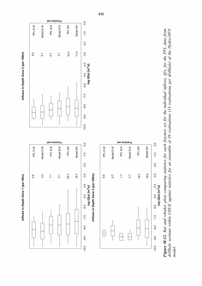
446
Infl
ow
s in
Dep
th Z
on
e 1
(p
er 5
0m
)
-10.
0-9
.0-8
.0-7
.0-6
.0-5
.0-4
.0-3
.0-2
.0-1
.00.
0
PF
L E
-W
Mod
el E
-W
PF
L N
-S
Mo
del N
-S
PF
L S
H
Mod
el S
H
Fracture set
log
(Q
/s)
[m2/s
]
7.1
4.2
5.6
5.1
22.3
18.4
Infl
ow
s in
Dep
th Z
on
e 2
(p
er 1
00m
)
-10.
0-9
.0-8
.0-7
.0-6
.0-5
.0-4
.0-3
.0-2
.0-1
.00.
0
PF
L E
-W
Mod
el E
-W
PF
L N
-S
Mo
del N
-S
PF
L S
H
Mod
el S
H
Fracture set
log
(Q
/s)
[m2/s
]
4.7
5.1
6.5
3.1
10.4
11.0
Infl
ow
s in
De
pth
Zo
ne
3 (
pe
r 25
0m
)
-10.
0-9
.0-8
.0-7
.0-6
.0-5
.0-4
.0-3
.0-2
.0-1
.00.
0
PF
L E
-W
Mod
el E
-W
PF
L N
-S
Mo
del N
-S
PF
L S
H
Mod
el S
H
Fracture set
log
(Q
/s)
[m2/s
]
1.7
6.7
8.6
2.7
18.3
19.0
Fig
ure
H-1
2. B
ar a
nd w
hisk
er p
lots
com
pari
ng s
tati
stic
s fo
r ea
ch f
ract
ure
set
for
the
indi
vidu
al i
nflo
ws,
Q/s
, fo
r th
e P
FL
dat
a fr
om
dril
lhol
e se
ctio
ns w
ithi
n C
HU
E a
gain
st s
tati
stic
s fo
r an
ens
embl
e of
39
real
isat
ions
(13
rea
lisa
tion
s pe
r dr
illh
ole)
of
the
Hyd
ro-D
FN
m
odel
.
446

447
De
pth
Zo
ne
1: S
ub
-Ho
rizo
nta
l
-11.
00
-10.
00
-9.0
0
-8.0
0
-7.0
0
-6.0
0
-5.0
0
-4.0
0
-3.0
0
-2-1
01
23
Lo
g1
0(r
) (m
)
Log10(T) (m2/s)
SC
SC
sp
read
C UC
UC
spr
ead
De
pth
Zo
ne
2:
Su
b-H
ori
zon
tal
-11.
00
-10.
00
-9.0
0
-8.0
0
-7.0
0
-6.0
0
-5.0
0
-4.0
0
-3.0
0
-2-1
01
23
Lo
g1
0(r
) (m
)
Log10(T) (m2/s)
SC
SC
spr
ea
dC U
CU
C s
pre
ad
De
pth
Zo
ne
3: S
ub
-Ho
rizo
nta
l
-11.
00
-10.
00
-9.0
0
-8.0
0
-7.0
0
-6.0
0
-5.0
0
-4.0
0
-3.0
0
-2-1
01
23
Lo
g1
0(r
) (m
)
Log10(T) (m2/s)
SC
SC
spr
ead
C UC
UC
spr
ead
Fig
ure
H-1
3. C
ompa
riso
n of
the
rela
tion
ship
bet
wee
n fr
actu
re tr
ansm
issi
vity
and
frac
ture
siz
e in
eac
h de
pth
zone
for
CH
UE
. The
plo
ts a
re
for
the
cali
brat
ed m
odel
of
sub-
hori
zont
al f
ract
ures
, us
ing
a po
wer
-law
fra
ctur
e si
ze d
istr
ibut
ion
(Cas
e A
) ba
sed
on o
pen
frac
ture
in
tens
itie
s. T
he p
lots
sho
w t
he c
entr
al t
rend
for
eac
h re
lati
onsh
ip t
oget
her
wit
h li
nes
at 1
sta
ndar
d de
viat
ion
abov
e an
d be
low
the
cen
tral
tr
end.
447

448
Total normalized flow to borehole section (Terzaghi corrected)
-4.8
-6.3
-6.0
-4.9
-6.3
-6.0
-8.5
-8.0
-7.5
-7.0
-6.5
-6.0
-5.5
-5.0
-4.5
-4.0
-3.5
DZ1 DZ2 DZ3 DZ4
Depth Zone
Lo
g [
Flo
w (
Q/s
)] [
m2 /s
]
Model
Data
Figure H-14. Comparison of the Terzaghi weighted sum of individual specific capacities, Q/s, for the PFL data from drillhole sections within CHUE normalised to the nominal thicknesses of each depth zone, against statistics for an ensemble over 13 realisations of 3 individual drillholes in the Hydro-DFN model. The model has a semi-correlated transmissivity with a power-law fracture size distribution (Case A) based on open fracture intensities. For the data, statistics are taken over the identified flowing fractures within each set. For the model, statistics are generated over 39 realisations. The total flows are normalised to the following lengths: Depth Zone 1 is 50 m, Depth Zone 2 is 100 m, Depth Zone 3 is 250 m, and Depth Zone 4 is 600 m.
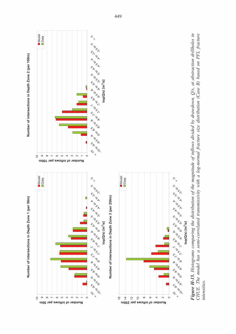
Nu
mb
er
of
inte
rse
cti
on
s i
n D
ep
th Z
on
e 1
(p
er
50m
)
012345678910
< -1
0 -10
to -9
.5 -9.5
to -9 -9
to -8
.5 -8.5
to -8 -8
to -7
.5 -7.5
to -7 -7
to -6
.5 -6.5
to -6 -6
to -5
.5 -5.5
to -5 -5
to -4
.5 -4.5
to -4 -4
to -3
.5 -3.5
to -3
> -3
log
(Q/s
) [m
2/s
]
Number of inflows per 50m
Mod
elD
ata
Nu
mb
er o
f in
ters
ecti
on
s in
Dep
th Z
on
e 2
(per
100
m)
012345678910
< -1
0 -10
to -9
.5 -9.5
to -9 -9
to -8
.5 -8.5
to -8 -8
to -7
.5 -7.5
to -7 -7
to -6
.5 -6.5
to -6 -6
to -5
.5 -5.5
to -5 -5
to -4
.5 -4.5
to -4 -4
to -3
.5 -3.5
to -3
> -3
log
(Q/s
) [m
2/s
]
Number of inflows per 100m
Mod
elD
ata
Nu
mb
er
of
inte
rse
cti
on
s i
n D
ep
th Z
on
e 3
(p
er
250
m)
0246810121416
< -1
0 -10
to -9
.5 -9.5
to -9 -9
to -8
.5 -8.5
to -8 -8
to -7
.5 -7.5
to -7 -7
to -6
.5 -6.5
to -6 -6
to -5
.5 -5.5
to -5 -5
to -4
.5 -4.5
to -4 -4
to -3
.5 -3.5
to -3
> -3
log
(Q/s
) [m
2/s
]
Number of inflows per 250m
Mod
elD
ata
Fig
ure
H-1
5. H
isto
gram
s co
mpa
ring
the
dist
ribu
tion
of th
e m
agni
tude
of i
nflo
ws
divi
ded
by d
raw
dow
n, Q
/s, a
t abs
trac
tion
drill
hole
s in
C
HU
E. T
he m
odel
has
a s
emi-c
orre
late
d tr
ansm
issi
vity
with
a l
og-n
orm
al f
ract
ure
size
dis
trib
utio
n (C
ase
B) b
ased
on
PFL
frac
ture
in
tens
ities
.
449
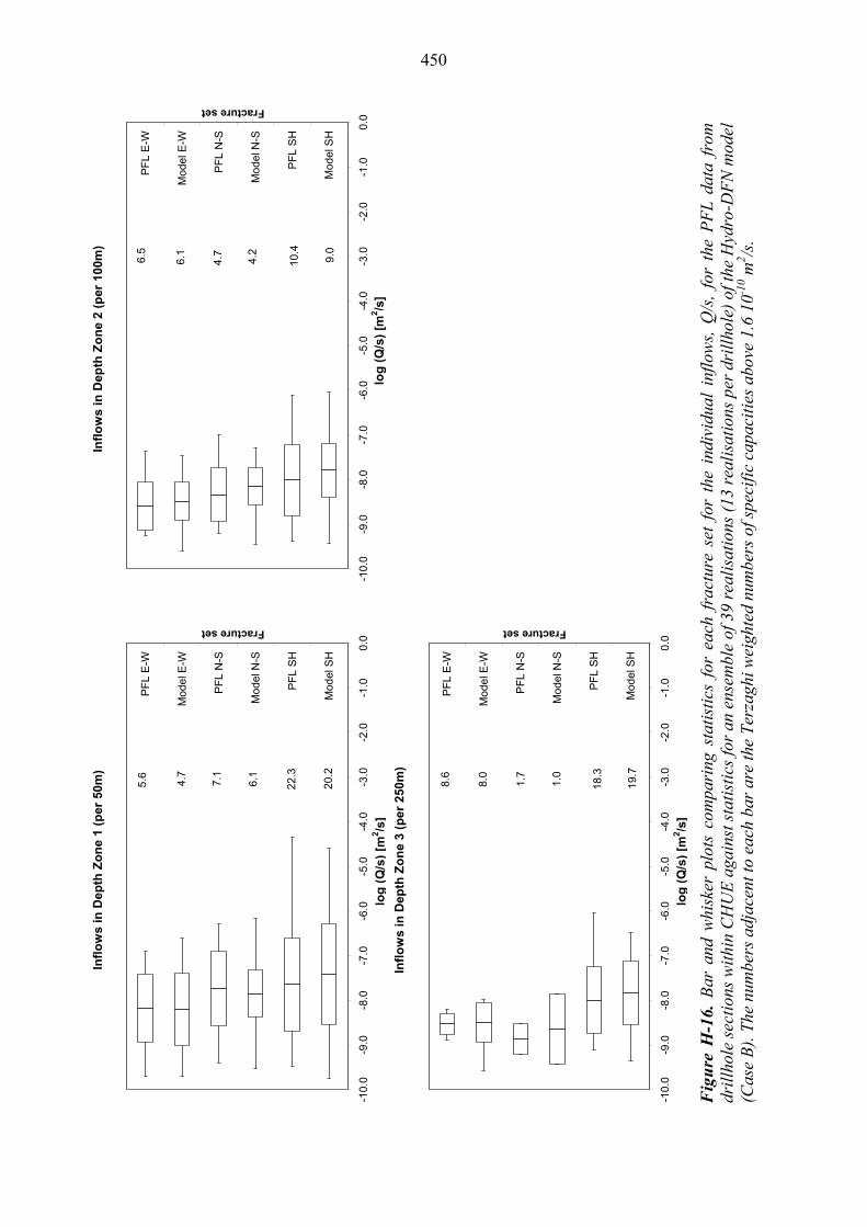
450
Infl
ow
s i
n D
epth
Zo
ne
1 (
pe
r 50
m)
-10.
0-9
.0-8
.0-7
.0-6
.0-5
.0-4
.0-3
.0-2
.0-1
.00
.0
PF
L E
-W
Mod
el E
-W
PF
L N
-S
Mod
el N
-S
PF
L S
H
Mod
el S
H
Fracture set
log
(Q
/s)
[m2/s
]
7.1
4.7
5.6 6.1
22.3
20.2
Infl
ow
s in
Dep
th Z
on
e 2
(p
er 1
00m
)
-10.
0-9
.0-8
.0-7
.0-6
.0-5
.0-4
.0-3
.0-2
.0-1
.00.
0
PF
L E
-W
Mod
el E
-W
PF
L N
-S
Mo
del N
-S
PF
L S
H
Mod
el S
H
Fracture set
log
(Q
/s)
[m2/s
]
4.7
6.1
6.5
4.2
10.4
9.0
Infl
ow
s in
Dep
th Z
on
e 3
(p
er
250
m)
-10.
0-9
.0-8
.0-7
.0-6
.0-5
.0-4
.0-3
.0-2
.0-1
.00
.0
PF
L E
-W
Mod
el E
-W
PF
L N
-S
Mod
el N
-S
PF
L S
H
Mod
el S
H
Fracture set
log
(Q
/s)
[m2/s
]
1.7
8.0
8.6
1.0
18.3
19.
7
Fig
ure
H-1
6. B
ar a
nd w
hisk
er p
lots
com
pari
ng s
tati
stic
s fo
r ea
ch f
ract
ure
set
for
the
indi
vidu
al i
nflo
ws,
Q/s
, fo
r th
e P
FL
dat
a fr
om
dril
lhol
e se
ctio
ns w
ithi
n C
HU
E a
gain
st s
tati
stic
s fo
r an
ens
embl
e of
39
real
isat
ions
(13
rea
lisa
tion
s pe
r dr
illh
ole)
of t
he H
ydro
-DF
N m
odel
(C
ase
B).
The
num
bers
adj
acen
t to
each
bar
are
the
Ter
zagh
i wei
ghte
d nu
mbe
rs o
f spe
cifi
c ca
paci
ties
abo
ve 1
.6 1
0-10 m
2 /s.
450

451
Total normalized flow to borehole section (Terzaghi corrected)
-4.9
-6.4
-6.1
-4.9
-6.3
-6.0
-8.5
-8.0
-7.5
-7.0
-6.5
-6.0
-5.5
-5.0
-4.5
-4.0
-3.5
DZ1 DZ2 DZ3 DZ4
Depth Zone
Lo
g [
Flo
w (
Q/s
)] [
m2 /s
]
Model
Data
Figure H-17. Comparison of the Terzaghi weighted sum of individual specific capacities, Q/s, for the PFL data from drillhole sections within CHUE normalised to the nominal thicknesses of each depth zone, against statistics for an ensemble over 13 realisations of 3 individual drillholes in the Hydro-DFN model. The model has a semi-correlated transmissivity with a log-normal fracture size distribution (Case B) based on PFL fracture intensities. For the data, statistics are taken over the identified flowing fractures within each set. For the model, statistics are generated over 39 realisations. The total flows are normalised to the following lengths: Depth Zone 1 is 50 m, Depth Zone 2 is 100 m, Depth Zone 3 is 250 m, and Depth Zone 4 is 600 m.
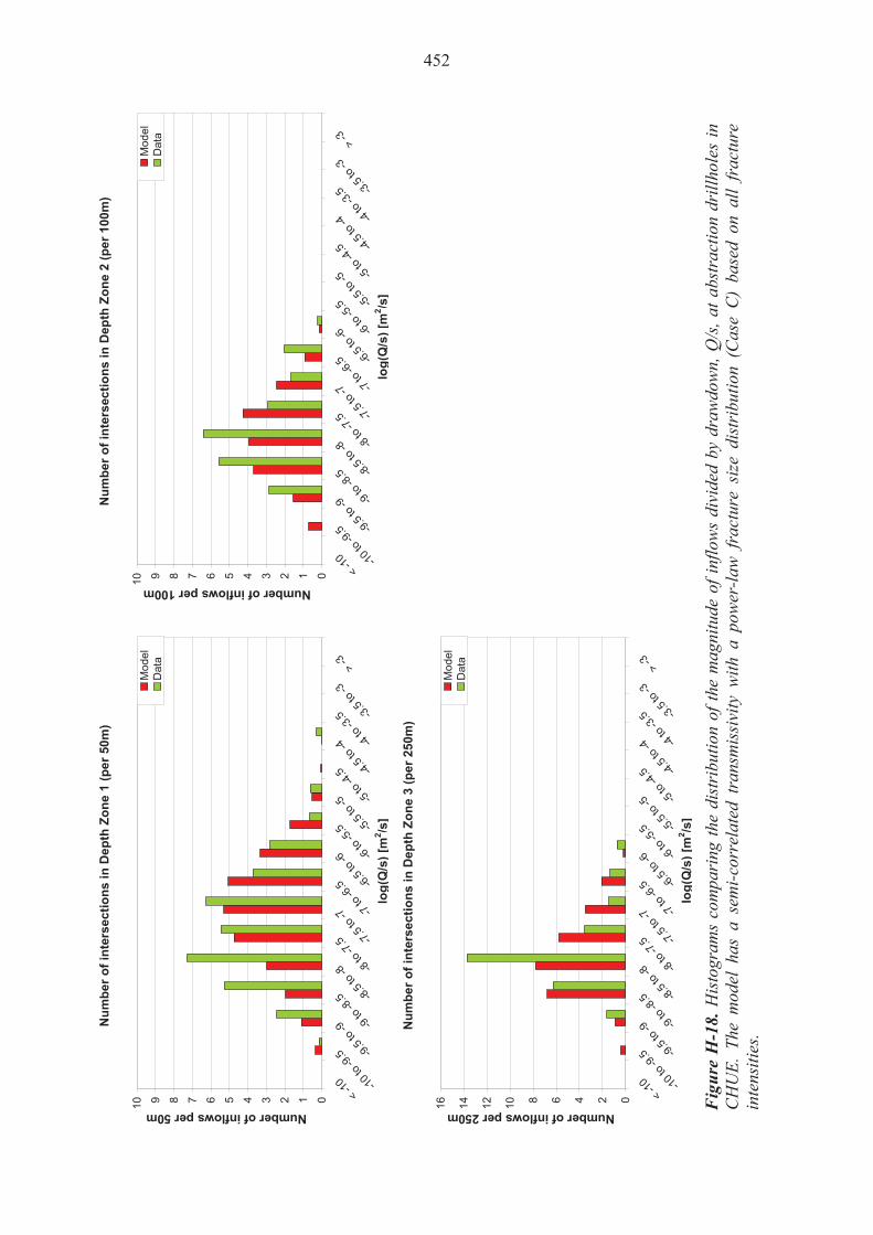
Nu
mb
er
of
inte
rse
cti
on
s i
n D
ep
th Z
on
e 1
(p
er
50m
)
012345678910
< -1
0 -10
to -9
.5 -9.5
to -9 -9
to -8
.5 -8.5
to -8 -8
to -7
.5 -7.5
to -7 -7
to -6
.5 -6.5
to -6 -6
to -5
.5 -5.5
to -5 -5
to -4
.5 -4.5
to -4 -4
to -3
.5 -3.5
to -3
> -3
log
(Q/s
) [m
2/s
]
Number of inflows per 50m
Mod
elD
ata
Nu
mb
er o
f in
ters
ecti
on
s in
Dep
th Z
on
e 2
(per
100
m)
012345678910
< -1
0 -10
to -9
.5 -9.5
to -9 -9
to -8
.5 -8.5
to -8 -8
to -7
.5 -7.5
to -7 -7
to -6
.5 -6.5
to -6 -6
to -5
.5 -5.5
to -5 -5
to -4
.5 -4.5
to -4 -4
to -3
.5 -3.5
to -3
> -3
log
(Q/s
) [m
2/s
]
Number of inflows per 100m
Mod
elD
ata
Nu
mb
er
of
inte
rse
cti
on
s i
n D
ep
th Z
on
e 3
(p
er
250
m)
0246810121416
< -1
0 -10
to -9
.5 -9.5
to -9 -9
to -8
.5 -8.5
to -8 -8
to -7
.5 -7.5
to -7 -7
to -6
.5 -6.5
to -6 -6
to -5
.5 -5.5
to -5 -5
to -4
.5 -4.5
to -4 -4
to -3
.5 -3.5
to -3
> -3
log
(Q/s
) [m
2/s
]
Number of inflows per 250m
Mod
elD
ata
Fig
ure
H-1
8. H
isto
gram
s co
mpa
ring
the
dist
ribu
tion
of th
e m
agni
tude
of i
nflo
ws
divi
ded
by d
raw
dow
n, Q
/s, a
t abs
trac
tion
drill
hole
s in
C
HU
E. T
he m
odel
has
a s
emi-c
orre
late
d tr
ansm
issi
vity
with
a p
ower
-law
fra
ctur
e si
ze d
istr
ibut
ion
(Cas
e C
) ba
sed
on a
ll fr
actu
re
inte
nsiti
es.
452

453
Infl
ow
s i
n D
epth
Zo
ne
1 (
pe
r 50
m)
-10.
0-9
.0-8
.0-7
.0-6
.0-5
.0-4
.0-3
.0-2
.0-1
.00
.0
PF
L E
-W
Mod
el E
-W
PF
L N
-S
Mod
el N
-S
PF
L S
H
Mod
el S
H
Fracture set
log
(Q
/s)
[m2/s
]
7.1
3.3
5.6 4.9
22.3
18.9
Infl
ow
s in
Dep
th Z
on
e 2
(p
er 1
00m
)
-10.
0-9
.0-8
.0-7
.0-6
.0-5
.0-4
.0-3
.0-2
.0-1
.00.
0
PF
L E
-W
Mod
el E
-W
PF
L N
-S
Mo
del N
-S
PF
L S
H
Mod
el S
H
Fracture set
log
(Q
/s)
[m2/s
]
4.7
5.2
6.5
3.2
10.4
9.2
Infl
ow
s in
Dep
th Z
on
e 3
(p
er
250
m)
-10.
0-9
.0-8
.0-7
.0-6
.0-5
.0-4
.0-3
.0-2
.0-1
.00
.0
PF
L E
-W
Mod
el E
-W
PF
L N
-S
Mod
el N
-S
PF
L S
H
Mod
el S
H
Fracture set
log
(Q
/s)
[m2/s
]
1.7
8.5
8.6
0.9
18.3
17.
8
Fig
ure
H-1
9. B
ar a
nd w
hisk
er p
lots
com
pari
ng s
tati
stic
s fo
r ea
ch f
ract
ure
set
for
the
indi
vidu
al i
nflo
ws,
Q/s
, fo
r th
e P
FL
dat
a fr
om
dril
lhol
e se
ctio
ns w
ithi
n C
HU
E a
gain
st s
tati
stic
s fo
r an
ens
embl
e of
39
real
isat
ions
(13
rea
lisa
tion
s pe
r dr
illh
ole)
of t
he H
ydro
-DF
N m
odel
(C
ase
C).
The
num
bers
adj
acen
t to
each
bar
are
the
Ter
zagh
i wei
ghte
d nu
mbe
rs o
f spe
cifi
c ca
paci
ties
abo
ve 1
.6 1
0-10 m
2 /s.
453

454
Total normalized flow to borehole section (Terzaghi corrected)
-5.0
-6.4 -6
.1
-4.9
-6.3
-6.0
-8.5
-8.0
-7.5
-7.0
-6.5
-6.0
-5.5
-5.0
-4.5
-4.0
-3.5
DZ1 DZ2 DZ3 DZ4
Depth Zone
Lo
g [
Flo
w (
Q/s
)] [
m2 /s
]
Model
Data
Figure H-20. Comparison of the Terzaghi weighted sum of individual specific capacities, Q/s, for the PFL data from drillhole sections within CHUE normalised to the nominal thicknesses of each depth zone, against statistics for an ensemble over 13 realisations of 3 individual drillholes in the Hydro-DFN model. The model has a semi-correlated transmissivity with a power-law fracture size distribution (Case C) based on all fracture intensities. For the data, statistics are taken over the identified flowing fractures within each set. For the model, statistics are generated over 39 realisations. The total flows are normalised to the following lengths: Depth Zone 1 is 50 m, Depth Zone 2 is 100 m, Depth Zone 3 is 250 m, and Depth Zone 4 is 600 m.

455
Case A
Table H-6. Summary of Hydro-DFN parameters for the simulations of flow in hydraulic domain CHUE, using a power-law size model (Case A).
Set Distribution of poles
Pole orientation F: trend, plunge, conc. B: (trend, plunge), conc.1, conc.2, rot.
Case A power-law (kr, r0) rmin = r0
rmax = 564 m
Intensity P32,open
Transmissivity model C: (a,b) SC: (a, b, σlog(T)) UC: (µ log(T), σ log(T))
(-, m) (m2/m3) T (m2s-1)
Depth Zone 1
EW Fisher (176.3, 0.4), 7.2 (2.65, 0.04) 0.43 C: (3.0E-8, 0.5) SC: (9.0E-9, 0.6, 0.5) UC: (1.0E-7, 0.5)
NS Fisher (95.3, 0.3), 6.9 (2.64, 0.04) 0.59 C: (1.0E-7, 0.45) SC: (1.0E-7, 0.4, 0.4) UC: (5.0E-7, 0.5)
SH Bingham (309.9, 78.6) -5.7, -4.0, 62.8o
(2.57, 0.04) 1.66 C: (2.0E-8, 1.2) SC: (2.0E-7, 0.7, 0.8) UC: (8.0E-7, 1.0)
Depth Zone 2
EW Fisher (176.3, 0.4), 7.2 (2.44, 0.04) 0.26 C: (1.0E-8, 0.3) SC: (8.0E-9, 0.2, 0.5) UC: (2.0E-8, 0.4)
NS Fisher (95.3, 0.3), 6.9 (2.49, 0.04) 0.24 C: (2.0E-8, 0.4) SC: (2.0E-8, 0.2, 0.7) UC: (5.0E-8, 0.4)
SH Bingham (309.9, 78.6) -5.7, -4.0, 62.8o
(2.55, 0.04) 0.81 C: (3.0E-8, 0.4) SC: (2.0E-8, 0.4, 0.5) UC: (1.0E-7, 0.5)
Depth Zone 3
EW Fisher (176.3, 0.4), 7.2 (2.48, 0.04) 0.22 C: (3.0E-9, 0.2) SC: (5.0E-9, 0.3, 0.2) UC: (8.0E-9, 0.2)
NS Fisher (95.3, 0.3), 6.9 (2.57, 0.04) 0.12 C: (2.0E-9, 0.2) SC: (1.0E-9, 0.2, 0.6) UC: (8.0E-9, 0.3)
SH Bingham (309.9, 78.6) -5.7, -4.0, 62.8o
(2.44, 0.04) 0.42 C: (4.5E-9, 0.8) SC: (1.0E-8, 0.6, 0.4) UC: (3.0E-8, 0.7)

456
Case B
Table H-7. Summary of Hydro-DFN parameters for the simulations of flow in hydraulic domain CHUE, using a log-normal size model (Case B).
Set Distribution of poles
Pole orientation F: trend, plunge, conc. B: (trend, plunge), conc.1, conc.2, rot.
Case B log-normal (mlog(r), slog(r)) rmin = 0.56m rmax = 564 m
Intensity P32,PFL
Transmissivity model SC: (a, b, σlog(T))
(-, m) (m2/m3) T (m2s-1)
Depth Zone 1
EW Fisher (176.3, 0.4), 7.2 (-0.77, 0.35) 0.11 SC: (3.0E-9, 0.7, 0.8)
NS Fisher (95.3, 0.3), 6.9 (-0.77, 0.35) 0.14 SC: (4.0E-9, 0.9, 0.2)
SH Bingham (309.9, 78.6)
-5.7, -4.0, 62.8o (-0.77, 0.35) 0.44 SC: (4.0E-8, 0.4, 1.4)
Depth Zone 2
EW Fisher (176.3, 0.4), 7.2 (-0.50, 0.35) 0.07 SC: (2.0E-9, 0.5, 0.2)
NS Fisher (95.3, 0.3), 6.9 (-0.50, 0.35) 0.05 SC: (3.0E-9, 0.6, 0.2)
SH Bingham (309.9, 78.6)
-5.7, -4.0, 62.8o (-0.50, 0.35) 0.10 SC: (9.0E-9, 0.6, 0.5)
Depth Zone 3
EW Fisher (176.3, 0.4), 7.2 (0.45, 0.25) 0.03 SC: (1.5E-9, 0.4, 0.1)
NS Fisher (95.3, 0.3), 6.9 (0.45, 0.25) 0.01 SC: (3.0E-8, 0.2, 0.2)
SH Bingham (309.9, 78.6)
-5.7, -4.0, 62.8o (0.45, 0.25) 0.07 SC: (2.0E-8, 0.2, 1.0)

457
Case C
Table H-8. Summary of Hydro-DFN parameters for the simulations of flow in hydraulic domain CHUE, using a power-law size model (r0=0.2, kr=2.59) with channels (Case C).
Set Distribution of poles
Pole orientation F: trend, plunge, conc. B: (trend, plunge), conc. 1, conc.2, rot.
Case C deletion parameters (d, a)
Intensity P32,open
Transmissivity model SC: (a, b, σlog(T))
(-, m) (m2/m3) T (m2s-1)
Depth Zone 1
EW Fisher (176.3, 0.4), 7.2 (15.5, 1.66) 0.80 SC: (1.0E-8, 0.5, 0.5)
NS Fisher (95.3, 0.3), 6.9 (15.25, 1.53) 1.11 SC: (1.0E-7, 0.45, 0.5)
SH Bingham (309.9, 78.6)
-5.7, -4.0, 62.8o (18.25, 3.02) 3.14 SC: (1.0E-7, 0.7, 0.8)
Depth Zone 2
EW Fisher (176.3, 0.4), 7.2 (23, 5.36) 0.66 SC: (8.0E-9, 0.15, 0.6)
NS Fisher (95.3, 0.3), 6.9 (14.6, 1.21) 0.59 SC: (2.0E-8, 0.2, 0.7)
SH Bingham (309.9, 78.6) -5.7, -4.0, 62.8o
(12, -0.07) 2.03 SC: (2.0E-8, 0.4, 0.6)
Depth Zone 3
EW Fisher (176.3, 0.4), 7.2 (8.5, -1.80) 1.00 SC: (4.5E-9, 0.3, 0.1)
NS Fisher (95.3, 0.3), 6.9 (6.9, -2.59) 0.55 SC: (1.5E-9, 0.2, 0.7)
SH Bingham (309.9, 78.6)
-5.7, -4.0, 62.8o (11.75, -0.20) 1.91 SC: (1.3E-8, 0.6, 0.5)
458
H.3 Flow calibration for hydraulic domain SHU
The results for the flow calibrations of hydraulic domain SHU are presented below.
Figure H-21, Figure H-25, and Figure H-28 illustrate histograms of the distribution of specific capacity, Q/s, for a bin size of half an order of magnitude compared with equivalent PFL data for each of the semi-correlated Case A, B and C fracture size distributions respectively. Corresponding correlation coefficients for these distributions, along with Case A correlated and uncorrelated models are summarised by depth zone in Table H-9.
Figure H-23 shows a comparison between the fracture transmissivity and the fracture size in each depth zone for the sub-horizontal (SH) fractures using a power-law fracture size distribution based on open fracture intensities.
Bar and whisker plots corresponding to semi-correlated transmissivities for fracture size distributions Case A, B and C are shown in Figure H-22, Figure H-26, and Figure H-29 respectively. These figures illustrate the comparison between the model and measured data for various statistical values of the specific capacity, Q/s. The centre of the bar indicates the mean value, the ends of the bar indicate ± one standard deviation and the error bars indicate the maximum and minimum values.
Figure H-24, Figure H-27, and Figure H-30 show histograms comparing the length normalised sum of the individual specific capacities (Q/s) with equivalent measured data for each of the fracture size distributions with semi-correlated transmissivities.
Table H-10 through Table H-12 summarise the transmissivity parameters found in the calibrated Case A, Case B and Case C fracture size distributions.
(Note that due to the lack of data in Depth Zone 4 of hydraulic domain SHU, no flow calibration results are presented. Instead, transmissivity parameters for CHUW have been assumed).
Table H-9. Correlation coefficients for the distribution of specific capacity, Q/s, between simulations and PFL data within domain SHU outside hydrozones. Values are given by depth zone for each model case considered.
Case Transmissivity
Model Depth Zone 1 Depth Zone 2 Depth Zone 3
A Correlated 0.94 0.87 0.81
A Semi-Correlated 0.98 0.89 0.88
A Uncorrelated 0.94 0.92 0.93
B Semi-Correlated 0.95 0.95 0.70
C Semi-Correlated 0.91 0.92 0.91

Nu
mb
er
of
inte
rse
cti
on
s i
n D
ep
th Z
on
e 1
(p
er
50m
)
012345678910
< -1
0 -10
to -9
.5 -9.5
to -9 -9
to -8
.5 -8.5
to -8 -8
to -7
.5 -7.5
to -7 -7
to -6
.5 -6.5
to -6 -6
to -5
.5 -5.5
to -5 -5
to -4
.5 -4.5
to -4 -4
to -3
.5 -3.5
to -3
> -3
log
(Q/s
) [m
2/s
]
Number of inflows per 50m
Mod
elD
ata
Nu
mb
er o
f in
ters
ecti
on
s in
Dep
th Z
on
e 2
(per
100
m)
024681012
< -1
0 -10
to -9
.5 -9.5
to -9 -9
to -8
.5 -8.5
to -8 -8
to -7
.5 -7.5
to -7 -7
to -6
.5 -6.5
to -6 -6
to -5
.5 -5.5
to -5 -5
to -4
.5 -4.5
to -4 -4
to -3
.5 -3.5
to -3
> -3
log
(Q/s
) [m
2/s
]
Number of inflows per 100m
Mod
elD
ata
Nu
mb
er
of
inte
rse
cti
on
s i
n D
ep
th Z
on
e 3
(p
er
250
m)
012345678910
< -1
0 -10
to -9
.5 -9.5
to -9 -9
to -8
.5 -8.5
to -8 -8
to -7
.5 -7.5
to -7 -7
to -6
.5 -6.5
to -6 -6
to -5
.5 -5.5
to -5 -5
to -4
.5 -4.5
to -4 -4
to -3
.5 -3.5
to -3
> -3
log
(Q/s
) [m
2/s
]
Number of inflows per 250m
Mod
elD
ata
Fig
ure
H-2
1. H
isto
gram
s co
mpa
ring
the
dist
ribu
tion
of th
e m
agni
tude
of i
nflo
ws
divi
ded
by d
raw
dow
n, Q
/s, a
t abs
trac
tion
drill
hole
s in
SH
U.
The
mod
el h
as a
sem
i-cor
rela
ted
tran
smis
sivi
ty w
ith a
pow
er-la
w f
ract
ure
size
dis
trib
utio
n (C
ase
A) b
ased
on
open
fra
ctur
e in
tens
ities
.
459

460
Infl
ow
s in
Dep
th Z
on
e 1
(p
er 5
0m
)
-10.
0-9
.0-8
.0-7
.0-6
.0-5
.0-4
.0-3
.0-2
.0-1
.00.
0
PF
L E
-W
Mod
el E
-W
PF
L N
-S
Mo
del N
-S
PF
L S
H
Mod
el S
H
Fracture set
log
(Q
/s)
[m2/s
]
6.2
4.1
6.6
5.6
24.5
21.8
Infl
ow
s in
Dep
th Z
on
e 2
(p
er 1
00m
)
-10.
0-9
.0-8
.0-7
.0-6
.0-5
.0-4
.0-3
.0-2
.0-1
.00.
0
PF
L E
-W
Mod
el E
-W
PF
L N
-S
Mo
del N
-S
PF
L S
H
Mod
el S
H
Fracture set
log
(Q
/s)
[m2/s
]
1.3
8.9
11.0
2.2
16.6
14.5
Infl
ow
s in
De
pth
Zo
ne
3 (
pe
r 25
0m
)
-10.
0-9
.0-8
.0-7
.0-6
.0-5
.0-4
.0-3
.0-2
.0-1
.00.
0
PF
L E
-W
Mod
el E
-W
PF
L N
-S
Mo
del N
-S
PF
L S
H
Mod
el S
H
Fracture set
log
(Q
/s)
[m2/s
]
2.3
0.6
1.4
2.6
18.5
16.4
Fig
ure
H-2
2. B
ar a
nd w
hisk
er p
lots
com
pari
ng s
tati
stic
s fo
r ea
ch f
ract
ure
set
for
the
indi
vidu
al i
nflo
ws,
Q/s
, fo
r th
e P
FL
dat
a fr
om
dril
lhol
e se
ctio
ns w
ithi
n SH
U a
gain
st s
tati
stic
s fo
r an
ens
embl
e of
39
real
isat
ions
(13
rea
lisa
tion
s pe
r dr
illh
ole)
of
the
Hyd
ro-D
FN
mod
el
(Cas
e A
).
460
461
De
pth
Zo
ne
1: S
ub
-Ho
rizo
nta
l
-11.
00
-10.
00
-9.0
0
-8.0
0
-7.0
0
-6.0
0
-5.0
0
-4.0
0
-3.0
0
-2-1
01
23
Lo
g1
0(r
) (m
)
Log10(T) (m2/s)
SC
SC
sp
read
C UC
UC
spr
ead
De
pth
Zo
ne
2:
Su
b-H
ori
zon
tal
-11.
00
-10.
00
-9.0
0
-8.0
0
-7.0
0
-6.0
0
-5.0
0
-4.0
0
-3.0
0
-2-1
01
23
Lo
g1
0(r
) (m
)
Log10(T) (m2/s)
SC
SC
spr
ea
dC U
CU
C s
pre
ad
De
pth
Zo
ne
3: S
ub
-Ho
rizo
nta
l
-11.
00
-10.
00
-9.0
0
-8.0
0
-7.0
0
-6.0
0
-5.0
0
-4.0
0
-3.0
0
-2-1
01
23
Lo
g1
0(r
) (m
)
Log10(T) (m2/s)
SC
SC
spr
ead
C UC
UC
spr
ead
Fig
ure
H-2
3. C
ompa
riso
n of
the
rel
atio
nshi
p be
twee
n fr
actu
re t
rans
mis
sivi
ty a
nd f
ract
ure
size
in
each
dep
th z
one
for
SHU
. The
plo
ts a
re
for
the
cali
brat
ed m
odel
of
sub-
hori
zont
al f
ract
ures
, us
ing
a po
wer
-law
fra
ctur
e si
ze d
istr
ibut
ion
(Cas
e A
) ba
sed
on o
pen
frac
ture
in
tens
itie
s. T
he p
lots
sho
w t
he c
entr
al t
rend
for
eac
h re
lati
onsh
ip t
oget
her
wit
h li
nes
at 1
sta
ndar
d de
viat
ion
abov
e an
d be
low
the
cen
tral
tr
end.
461
462
Total normalized flow to borehole section (Terzaghi corrected)
-4.9
-6.3
-6.6
-5.0
-6.4
-6.6
-8.5
-8.0
-7.5
-7.0
-6.5
-6.0
-5.5
-5.0
-4.5
-4.0
-3.5
DZ1 DZ2 DZ3 DZ4
Depth Zone
Lo
g [
Flo
w (
Q/s
)] [
m2 /s
]
Model
Data
Figure H-24. Comparison of the Terzaghi weighted sum of individual specific capacities, Q/s, for the PFL data from drillhole sections within SHU normalised to the nominal thicknesses of each depth zone, against statistics for an ensemble over 13 realisations of 3 individual drillholes in the Hydro-DFN model. The model has a semi-correlated transmissivity with a power-law fracture size distribution (Case A) based on open fracture intensities. For the data, statistics are taken over the identified flowing fractures within each set. For the model, statistics are generated over 39 realisations. The total flows are normalised to the following lengths: Depth Zone 1 is 50 m, Depth Zone 2 is 100 m, Depth Zone 3 is 250 m, and Depth Zone 4 is 600 m.

Nu
mb
er
of
inte
rse
cti
on
s i
n D
ep
th Z
on
e 1
(p
er
50m
)
012345678910
< -1
0 -10
to -9
.5 -9.5
to -9 -9
to -8
.5 -8.5
to -8 -8
to -7
.5 -7.5
to -7 -7
to -6
.5 -6.5
to -6 -6
to -5
.5 -5.5
to -5 -5
to -4
.5 -4.5
to -4 -4
to -3
.5 -3.5
to -3
> -3
log
(Q/s
) [m
2/s
]
Number of inflows per 50m
Mod
elD
ata
Nu
mb
er o
f in
ters
ecti
on
s in
Dep
th Z
on
e 2
(per
100
m)
024681012
< -1
0 -10
to -9
.5 -9.5
to -9 -9
to -8
.5 -8.5
to -8 -8
to -7
.5 -7.5
to -7 -7
to -6
.5 -6.5
to -6 -6
to -5
.5 -5.5
to -5 -5
to -4
.5 -4.5
to -4 -4
to -3
.5 -3.5
to -3
> -3
log
(Q/s
) [m
2/s
]
Number of inflows per 100m
Mod
elD
ata
Nu
mb
er
of
inte
rse
cti
on
s i
n D
ep
th Z
on
e 3
(p
er
250
m)
012345678910
< -1
0 -10
to -9
.5 -9.5
to -9 -9
to -8
.5 -8.5
to -8 -8
to -7
.5 -7.5
to -7 -7
to -6
.5 -6.5
to -6 -6
to -5
.5 -5.5
to -5 -5
to -4
.5 -4.5
to -4 -4
to -3
.5 -3.5
to -3
> -3
log
(Q/s
) [m
2/s
]
Number of inflows per 250m
Mod
elD
ata
Fig
ure
H-2
5. H
isto
gram
s co
mpa
ring
the
dist
ribu
tion
of th
e m
agni
tude
of i
nflo
ws
divi
ded
by d
raw
dow
n, Q
/s, a
t abs
trac
tion
drill
hole
s in
SH
U.
The
mod
el h
as a
sem
i-cor
rela
ted
tran
smis
sivi
ty w
ith a
log
-nor
mal
fra
ctur
e si
ze d
istr
ibut
ion
(Cas
e B)
bas
ed o
n PF
L fr
actu
re
inte
nsiti
es.
463

464
Infl
ow
s in
Dep
th Z
on
e 1
(p
er 5
0m
)
-10.
0-9
.0-8
.0-7
.0-6
.0-5
.0-4
.0-3
.0-2
.0-1
.00.
0
PF
L E
-W
Mod
el E
-W
PF
L N
-S
Mo
del N
-S
PF
L S
H
Mod
el S
H
Fracture set
log
(Q
/s)
[m2/s
]
6.2
6.0
6.6
5.8
24.5
23.5
Infl
ow
s in
Dep
th Z
on
e 2
(p
er 1
00m
)
-10.
0-9
.0-8
.0-7
.0-6
.0-5
.0-4
.0-3
.0-2
.0-1
.00.
0
PF
L E
-W
Mod
el E
-W
PF
L N
-S
Mo
del N
-S
PF
L S
H
Mod
el S
H
Fracture set
log
(Q
/s)
[m2/s
]
1.3
8.4
11.0
0.8
16.6
15.6
Infl
ow
s in
De
pth
Zo
ne
3 (
pe
r 25
0m
)
-10.
0-9
.0-8
.0-7
.0-6
.0-5
.0-4
.0-3
.0-2
.0-1
.00.
0
PF
L E
-W
Mod
el E
-W
PF
L N
-S
Mo
del N
-S
PF
L S
H
Mod
el S
H
Fracture set
log
(Q
/s)
[m2/s
]
2.3
1.4
1.4
2.3
18.5
15.0
Fig
ure
H-2
6. B
ar a
nd w
hisk
er p
lots
com
pari
ng s
tati
stic
s fo
r ea
ch f
ract
ure
set
for
the
indi
vidu
al i
nflo
ws,
Q/s
, fo
r th
e P
FL
dat
a fr
om
dril
lhol
e se
ctio
ns w
ithi
n SH
U a
gain
st s
tati
stic
s fo
r an
ens
embl
e of
39
real
isat
ions
(13
rea
lisa
tion
s pe
r dr
illh
ole)
of
the
Hyd
ro-D
FN
mod
el
(Cas
e B
). T
he n
umbe
rs a
djac
ent t
o ea
ch b
ar a
re th
e T
erza
ghi w
eigh
ted
num
bers
of s
peci
fic
capa
citi
es a
bove
1.6
10-1
0 m2 /s
.
464

465
Total normalized flow to borehole section (Terzaghi corrected)
-5.0
-6.4
-6.7
-5.0
-6.4
-6.6
-8.5
-8.0
-7.5
-7.0
-6.5
-6.0
-5.5
-5.0
-4.5
-4.0
-3.5
DZ1 DZ2 DZ3 DZ4
Depth Zone
Lo
g [
Flo
w (
Q/s
)] [
m2 /s
]
Model
Data
Figure H-27. Comparison of the Terzaghi weighted sum of individual specific capacities, Q/s, for the PFL data from drillhole sections within SHU normalised to the nominal thicknesses of each depth zone, against statistics for an ensemble over 13 realisations of 3 individual drillholes in the Hydro-DFN model. The model has a semi-correlated transmissivity with a log-normal fracture size distribution (Case B) based on PFL fracture intensities. For the data, statistics are taken over the identified flowing fractures within each set. For the model, statistics are generated over 39 realisations. The total flows are normalised to the following lengths: Depth Zone 1 is 50 m, Depth Zone 2 is 100 m, Depth Zone 3 is 250 m, and Depth Zone 4 is 600 m.
Nu
mb
er
of
inte
rse
cti
on
s i
n D
ep
th Z
on
e 1
(p
er
50m
)
012345678910
< -1
0 -10
to -9
.5 -9.5
to -9 -9
to -8
.5 -8.5
to -8 -8
to -7
.5 -7.5
to -7 -7
to -6
.5 -6.5
to -6 -6
to -5
.5 -5.5
to -5 -5
to -4
.5 -4.5
to -4 -4
to -3
.5 -3.5
to -3
> -3
log
(Q/s
) [m
2/s
]
Number of inflows per 50m
Mod
elD
ata
Nu
mb
er o
f in
ters
ecti
on
s in
Dep
th Z
on
e 2
(per
100
m)
024681012
< -1
0 -10
to -9
.5 -9.5
to -9 -9
to -8
.5 -8.5
to -8 -8
to -7
.5 -7.5
to -7 -7
to -6
.5 -6.5
to -6 -6
to -5
.5 -5.5
to -5 -5
to -4
.5 -4.5
to -4 -4
to -3
.5 -3.5
to -3
> -3
log
(Q/s
) [m
2/s
]
Number of inflows per 100m
Mod
elD
ata
Nu
mb
er
of
inte
rse
cti
on
s i
n D
ep
th Z
on
e 3
(p
er
250
m)
012345678910
< -1
0 -10
to -9
.5 -9.5
to -9 -9
to -8
.5 -8.5
to -8 -8
to -7
.5 -7.5
to -7 -7
to -6
.5 -6.5
to -6 -6
to -5
.5 -5.5
to -5 -5
to -4
.5 -4.5
to -4 -4
to -3
.5 -3.5
to -3
> -3
log
(Q/s
) [m
2/s
]
Number of inflows per 250m
Mod
elD
ata
Fig
ure
H-2
8. H
isto
gram
s co
mpa
ring
the
dist
ribu
tion
of th
e m
agni
tude
of i
nflo
ws
divi
ded
by d
raw
dow
n, Q
/s, a
t abs
trac
tion
drill
hole
s in
SH
U. T
he m
odel
has
a se
mi-c
orre
late
d tr
ansm
issi
vity
with
a p
ower
-law
frac
ture
size
dis
trib
utio
n (C
ase
C) b
ased
on
all f
ract
ure
inte
nsiti
es.
466
467
Infl
ow
s in
Dep
th Z
on
e 1
(p
er 5
0m
)
-10.
0-9
.0-8
.0-7
.0-6
.0-5
.0-4
.0-3
.0-2
.0-1
.00.
0
PF
L E
-W
Mod
el E
-W
PF
L N
-S
Mo
del N
-S
PF
L S
H
Mod
el S
H
Fracture set
log
(Q
/s)
[m2/s
]
6.2
7.3
6.6
6.5
24.5
17.3
Infl
ow
s in
Dep
th Z
on
e 2
(p
er 1
00m
)
-10.
0-9
.0-8
.0-7
.0-6
.0-5
.0-4
.0-3
.0-2
.0-1
.00.
0
PF
L E
-W
Mod
el E
-W
PF
L N
-S
Mo
del N
-S
PF
L S
H
Mod
el S
H
Fracture set
log
(Q
/s)
[m2/s
]
1.3
8.1
11.0
0.9
16.6
12.3
Infl
ow
s in
De
pth
Zo
ne
3 (
pe
r 25
0m
)
-10.
0-9
.0-8
.0-7
.0-6
.0-5
.0-4
.0-3
.0-2
.0-1
.00.
0
PF
L E
-W
Mod
el E
-W
PF
L N
-S
Mo
del N
-S
PF
L S
H
Mod
el S
H
Fracture set
log
(Q
/s)
[m2/s
]
2.3
0.6
1.4
3.3
18.5
17.4
Fig
ure
H-2
9. B
ar a
nd w
hisk
er p
lots
com
pari
ng s
tati
stic
s fo
r ea
ch f
ract
ure
set
for
the
indi
vidu
al i
nflo
ws,
Q/s
, fo
r th
e P
FL
dat
a fr
om
dril
lhol
e se
ctio
ns w
ithi
n SH
U a
gain
st s
tati
stic
s fo
r an
ens
embl
e of
39
real
isat
ions
(13
rea
lisa
tion
s pe
r dr
illh
ole)
of
the
Hyd
ro-D
FN
mod
el
(Cas
e C
).T
he n
umbe
rs a
djac
ent t
o ea
ch b
ar a
re th
e T
erza
ghi w
eigh
ted
num
bers
of s
peci
fic
capa
citi
es a
bove
1.6
10-1
0 m2 /s
.
467

468
Total normalized flow to borehole section (Terzaghi corrected)
-5.0
-6.4
-6.7
-5.0
-6.4
-6.6
-8.5
-8.0
-7.5
-7.0
-6.5
-6.0
-5.5
-5.0
-4.5
-4.0
-3.5
DZ1 DZ2 DZ3 DZ4
Depth Zone
Lo
g [
Flo
w (
Q/s
)] [
m2 /s
]
Model
Data
Figure H-30. Comparison of the Terzaghi weighted sum of individual specific capacities, Q/s, for the PFL data from drillhole sections within SHU normalised to the nominal thicknesses of each depth zone, against statistics for an ensemble over 13 realisations of 3 individual drillholes in the Hydro-DFN model. The model has a semi-correlated transmissivity with a power-law fracture size distribution (Case C) based on all fracture intensities. For the data, statistics are taken over the identified flowing fractures within each set. For the model, statistics are generated over 39 realisations. The total flows are normalised to the following lengths: Depth Zone 1 is 50 m, Depth Zone 2 is 100 m, Depth Zone 3 is 250 m, and Depth Zone 4 is 600 m.
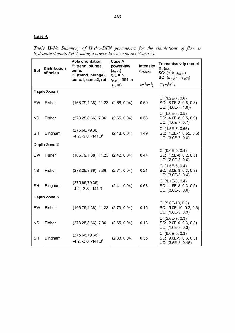
469
Case A
Table H-10. Summary of Hydro-DFN parameters for the simulations of flow in hydraulic domain SHU, using a power-law size model (Case A).
Set Distribution of poles
Pole orientation F: trend, plunge, conc. B: (trend, plunge), conc.1, conc.2, rot.
Case A power-law (kr, r0) rmin = r0
rmax = 564 m
Intensity P32,open
Transmissivity model C: (a,b) SC: (a, b, σlog(T)) UC: (µ log(T), σ log(T))
(-, m) (m2/m3) T (m2s-1)
Depth Zone 1
EW Fisher (166.79,1.38), 11.23 (2.66, 0.04) 0.59 C: (1.2E-7, 0.6) SC: (8.0E-8, 0.6, 0.8) UC: (4.0E-7, 1.0))
NS Fisher (278.25,8.66), 7.36 (2.65, 0.04) 0.53 C: (6.0E-8, 0.5) SC: (4.0E-8, 0.5, 0.9) UC: (1.0E-7, 0.7)
SH Bingham (275.66,79.36)
-4.2, -3.8, -141.3o (2.48, 0.04) 1.49
C: (1.5E-7, 0.65) SC: (1.3E-7, 0.65, 0.5)UC: (3.0E-7, 0.8)
Depth Zone 2
EW Fisher (166.79,1.38), 11.23 (2.42, 0.04) 0.44 C: (9.0E-9, 0.4) SC: (1.5E-8, 0.2, 0.5) UC: (2.0E-8, 0.6)
NS Fisher (278.25,8.66), 7.36 (2.71, 0.04) 0.21 C: (1.5E-8, 0.4) SC: (3.0E-8, 0.3, 0.3) UC: (3.0E-8, 0.4)
SH Bingham (275.66,79.36)
-4.2, -3.8, -141.3o (2.41, 0.04) 0.63
C: (1.1E-8, 0.4) SC: (1.5E-8, 0.3, 0.5) UC: (3.0E-8, 0.6)
Depth Zone 3
EW Fisher (166.79,1.38), 11.23 (2.73, 0.04) 0.15 C: (5.0E-10, 0.3) SC: (5.0E-10, 0.3, 0.3)UC: (1.0E-9, 0.3)
NS Fisher (278.25,8.66), 7.36 (2.65, 0.04) 0.13 C: (2.0E-9, 0.3) SC: (2.0E-9, 0.3, 0.3) UC: (1.0E-8, 0.3)
SH Bingham (275.66,79.36)
-4.2, -3.8, -141.3o (2.33, 0.04) 0.35
C: (9.0E-9, 0.3) SC: (9.0E-9, 0.3, 0.3) UC: (3.5E-8, 0.45)
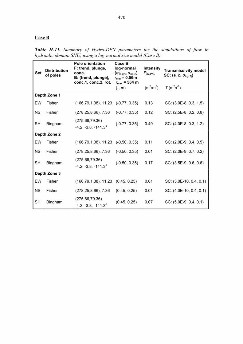
470
Case B
Table H-11. Summary of Hydro-DFN parameters for the simulations of flow in hydraulic domain SHU, using a log-normal size model (Case B).
Set Distribution of poles
Pole orientation F: trend, plunge, conc. B: (trend, plunge), conc.1, conc.2, rot.
Case B log-normal (mlog(r), slog(r)) rmin = 0.56m rmax = 564 m
Intensity P32,PFL
Transmissivity model SC: (a, b, σlog(T))
(-, m) (m2/m3) T (m2s-1)
Depth Zone 1
EW Fisher (166.79,1.38), 11.23 (-0.77, 0.35) 0.13 SC: (3.0E-8, 0.3, 1.5)
NS Fisher (278.25,8.66), 7.36 (-0.77, 0.35) 0.12 SC: (2.5E-8, 0.2, 0.8)
SH Bingham (275.66,79.36)
-4.2, -3.8, -141.3o (-0.77, 0.35) 0.49 SC: (4.0E-8, 0.3, 1.2)
Depth Zone 2
EW Fisher (166.79,1.38), 11.23 (-0.50, 0.35) 0.11 SC: (2.0E-9, 0.4, 0.5)
NS Fisher (278.25,8.66), 7.36 (-0.50, 0.35) 0.01 SC: (2.0E-9, 0.7, 0.2)
SH Bingham (275.66,79.36)
-4.2, -3.8, -141.3o (-0.50, 0.35) 0.17 SC: (3.5E-9, 0.6, 0.6)
Depth Zone 3
EW Fisher (166.79,1.38), 11.23 (0.45, 0.25) 0.01 SC: (3.0E-10, 0.4, 0.1)
NS Fisher (278.25,8.66), 7.36 (0.45, 0.25) 0.01 SC: (4.0E-10, 0.4, 0.1)
SH Bingham (275.66,79.36)
-4.2, -3.8, -141.3o (0.45, 0.25) 0.07 SC: (5.0E-9, 0.4, 0.1)

471
Case C
Table H-12. Summary of Hydro-DFN parameters for the simulations of flow in hydraulic domain SHU, using a power-law size model (r0=0.2, kr=2.59) with channels (Case C).
Set Distribution of poles
Pole orientation F: trend, plunge, conc. B: (trend, plunge), conc. 1, conc.2, rot.
Case C deletion parameters (d, a)
Intensity P32,open
Transmissivity model SC: (a, b, σlog(T))
(-, m) (m2/m3) T (m2s-1)
Depth Zone 1
EW Fisher (166.79,1.38), 11.23 (19, 3.39) 1.12 SC: (5.0E-8, 0.6, 0.8)
NS Fisher (278.25,8.66), 7.36 (17, 2.40) 0.99 SC: (3.0E-8, 0.5, 0.9)
SH Bingham (275.66,79.36)
-4.2, -3.8, -141.3o (21, 4.37) 2.82 SC: (5.0E-8, 0.65, 1.0)
Depth Zone 2
EW Fisher (166.79,1.38), 11.23 (17, 2.40) 1.11 SC: (1.2E-8, 0.2, 0.5)
NS Fisher (278.25,8.66), 7.36 (10, -1.06) 0.52 SC: (1.6E-8, 0.15, 0.4)
SH Bingham (275.66,79.36)
-4.2, -3.8, -141.3o (17, 2.40) 1.57 SC: (2.0E-8, 0.3, 0.6)
Depth Zone 3
EW Fisher (166.79,1.38), 11.23 (5, -3.53) 0.70 SC: (5.0E-10, 0.3, 0.3)
NS Fisher (278.25,8.66), 7.36 (8, -2.05) 0.57 SC: (2.0E-9, 0.3, 0.3)
SH Bingham (275.66,79.36)
-4.2, -3.8, -141.3o (14, 0.92) 1.59 SC: (2.0E-8, 0.2, 0.2)

472
473
APPENDIX I: HYDRAULIC TESTING UNIT (HTU) REFERENCES
Hämäläinen, H. 2009. Hydraulic Conductivity Measurements with HTU at Eurajoki, Olkiluoto, Drillholes OL-KR22, OL-KR27 and OL-KR41 in 2007. Eurajoki, Finland: Posiva Oy. 62 p + disc. Working Report 2009-105.
Hämäläinen, H. 2009. Hydraulic Conductivity Measurements with HTU at Eurajoki, Olkiluoto, Drillholes OL-KR40, OL-KR42 and OL-KR45 in 2008. Eurajoki, Finland: Posiva Oy. 82 p + disc. Working Report 2009-104.
Hämäläinen, H. 2009. Monitoring Hydraulic Conductivity with HTU at Eurajoki, Olkiluoto, Drillholes OL-KR31 and OL-KR32 in 2008. Eurajoki, Finland. Posiva Oy. 52 p + disc. Working Report 2009-50.
Hämäläinen, H. 2009. Monitoring Hydraulic Conductivity with HTU at Eurajoki, Olkiluoto, Drillholes OL-KR31 and OL-KR32 in 2008. Eurajoki, Finland. Posiva Oy. 52 p + disc. Working Report 2009-50.
Hämäläinen, H. 1991c. Hydraulical Testing at Olkiluoto, Drillhole KR1 (in Finnish with an English abstract). Helsinki, Finland: Teollisuuden Voima Oy. xx p. TVO/Site Investigations Work Report 91-04.
Hämäläinen, H. 1991d. Hydraulical Testing at Olkiluoto, Drillholes KR2, KR3, KR4 and KR5 (in Finnish with an English abstract). Helsinki, Finland: Teollisuuden Voima Oy. xx p. TVO/Site Investigations Work Report 91-05.
Hämäläinen, H. 1997b. Hydraulic Conductivity Measurements at Olkiluoto, Drillhole OL-KR1 (in Finnish with an English abstract). Helsinki, Finland: Posiva Oy. xx p. Working Report 97-03.
Hämäläinen, H. 1997c. Hydraulic Conductivity Measurements at Eurajoki, Olkiluoto, Drillhole OL-KR2 (in Finnish with an English abstract). Helsinki, Finland: Posiva Oy. xx p. Working Report 97-21.
Hämäläinen, H. 1997d. Hydraulic Conductivity Measurements at Eurajoki, Olkiluoto, Drillhole OL-KR4 (in Finnish with an English abstract). Helsinki, Finland: Posiva Oy. 22 p. Working Report 97-45.
Hämäläinen, H. 1997e. Hydraulic Conductivity Measurements at Eurajoki, Olkiluoto, Drillhole OL-KR8 (in Finnish with an English abstract). Helsinki, Finland: Posiva Oy. 22 p. Working Report 97-46.
Hämäläinen, H. 1997f. Hydraulic Conductivity Measurements at Eurajoki, Olkiluoto, Drillhole OL-KR10 (in Finnish with an English abstract). Helsinki, Finland: Posiva Oy. 22 p. Working Report 97-47.
Hämäläinen, H. 2003a. Complementary Hydraulic Conductivity Measurements at Eurajoki, Olkiluoto, Drillhole OL-KR1, Volume 1 and 2 (in Finnish with an English abstract). Eurajoki, Finland: Posiva Oy. 20 p. Working Report 2003-27.

474
Hämäläinen, H. 2003b. Complementary Hydraulic Conductivity Measurements at Eurajoki, Olkiluoto, Drillhole OL-KR7, Volumes 1 and 2 (in Finnish with an English abstract). Eurajoki, Finland: Posiva Oy. 20 p. Working Report 2003-47.
Hämäläinen, H. 2003c. Complementary Hydraulic Conductivity Measurements at Eurajoki, Olkiluoto, Drillhole OL-KR10, Volumes 1 and 2 (in Finnish with an English abstract). Eurajoki, Finland: Posiva Oy. 20 p. Working Report 2003-54.
Hämäläinen, H. 2004a. Hydraulic Conductivity Measurements with HTU at Eurajoki, Olkiluoto, Drillhole OL-KR12. Eurajoki, Finland: Posiva Oy. 23 p. Working Report 2004-14.
Hämäläinen, H. 2004b. Hydraulic Conductivity Measurements with HTU at Eurajoki Olkiluoto, Drillhole OL-KR13, Volumes 1 and 2. Eurajoki, Finland: Posiva Oy. No page numbering. Working Report 2004-40.
Hämäläinen, H. 2004b. Hydraulic Conductivity Measurements with HTU at Eurajoki Olkiluoto, Drillhole OL-KR13, Volume 1. Eurajoki, Finland: Posiva Oy. 57 p + app. Working Report 2004-40.
Hämäläinen, H. 2004b. Hydraulic Conductivity Measurements with HTU at Eurajoki Olkiluoto, Drillhole OL-KR13, Volume 2. Eurajoki, Finland: Posiva Oy. 57 p + app. Working Report 2004-40.
Hämäläinen, H. 2004c. Hydraulic Conductivity Measurements with HTU at Eurajoki Olkiluoto, Drillhole OL-KR14, Volumes 1 and 2. Eurajoki, Finland: Posiva Oy. xx p. Working Report 2004-42.
Hämäläinen, H. 2004c. Hydraulic Conductivity Measurements with HTU at Eurajoki Olkiluoto, Drillhole OL-KR14, Volume 1. Eurajoki, Finland: Posiva Oy. 64 p. + app. Working Report 2004-42.
Hämäläinen, H. 2004c. Hydraulic Conductivity Measurements with HTU at Eurajoki Olkiluoto, Drillhole OL-KR14, Volume 2. Eurajoki, Finland: Posiva Oy. NN p. Working Report 2004-42.
Hämäläinen, H. 2006a. Hydraulic Conductivity Measurements with HTU at Eurajoki Olkiluoto, Drillhole OL-KR15 and OL-KR15B, Volumes 1 and 2. Eurajoki, Finland: Posiva Oy. xx p. Working Report 2005-23.
Hämäläinen, H. 2006a. Hydraulic Conductivity Measurements with HTU at Eurajoki Olkiluoto, Drillhole OL-KR15 and OL-KR15B, Volume 1. Eurajoki, Finland: Posiva Oy. 66 p. + app. Working Report 2005-23.
Hämäläinen, H. 2006a. Hydraulic Conductivity Measurements with HTU at Eurajoki Olkiluoto, Drillhole OL-KR15 and OL-KR15B, Volume 2. Eurajoki, Finland: Posiva Oy. NN p. Working Report 2005-23.
Hämäläinen, H. 2006b. Hydraulic Crosshole Interference Tests at Olkiluoto, Eurajoki in 2004 HTU-measurements in drillholes KR14, KR17 and KR18. Eurajoki, Finland: Posiva Oy. 17 p. Working Report 2006-02.
475
Hämäläinen, H. 2006b. Hydraulic Crosshole Interference Tests at Olkiluoto, Eurajoki in 2004 HTU-measurements in drillholes KR14, KR17 and KR18. Eurajoki, Finland: Posiva Oy. 17 p. Working Report 2006-02.
Hämäläinen, H. 2006c. Hydraulic Conductivity Measurements with HTU at Eurajoki Olkiluoto, Drillhole OL-KR16, OL-KR16B, OL-KR17, OL-KR17B, OL-KR18 and OL-KR18B in 2004, Volumes 1 and 2. Eurajoki, Finland: Posiva Oy. xx p. Working Report 2006-04.
Hämäläinen, H. 2006c. Hydraulic Conductivity Measurements with HTU at Eurajoki Olkiluoto, Drillhole OL-KR16, OL-KR16B, OL-KR17, OL-KR17B, OL-KR18 and OL-KR18B in 2004, Volume 2. Eurajoki, Finland: Posiva Oy. NN p. Working Report 2006-04.
Hämäläinen, H. 2006c. Hydraulic Conductivity Measurements with HTU at Eurajoki Olkiluoto, Drillhole OL-KR16, OL-KR16B, OL-KR17, OL-KR17B, OL-KR18 and OL-KR18B in 2004, Volume 1. Eurajoki, Finland: Posiva Oy. NN p. Working Report 2006-04.
Hämäläinen, H. 2006d. Hydraulic Conductivity Measurements with HTU at Eurajoki, Olkiluoto, Drillhole OL-KR2 in 2003, Volumes 1 and 2. Eurajoki, Finland: Posiva Oy. xx p. Working Report 2006-10.
Hämäläinen, H. 2006d. Hydraulic Conductivity Measurements with HTU at Eurajoki, Olkiluoto, Drillhole OL-KR2 in 2003, Volume 1. Eurajoki, Finland: Posiva Oy. 42 p. + app. Working Report 2006-10.
Hämäläinen, H. 2006d. Hydraulic Conductivity Measurements with HTU at Eurajoki, Olkiluoto, Drillhole OL-KR2 in 2003, Volume 2. Eurajoki, Finland: Posiva Oy. xx p. Working Report 2006-10.
Hämäläinen, H. 2006e. Monitoring Measurements with HTU at Eurajoki, Olkiluoto, Drillholes OL-KR 4, 8, 28 and 31, Year 2005. Eurajoki, Finland: Posiva Oy. 49 p. Working Report 2006-23.
Hämäläinen, H. 2006e. Monitoring Measurements with HTU at Eurajoki, Olkiluoto, Drillholes OL-KR 4, 8, 28 and 31, Year 2005. Eurajoki, Finland: Posiva Oy. 49 p. Working Report 2006-23.
Hämäläinen, H. 2006f. Hydraulic Conductivity Measurements with HTU at Eurajoki Olkiluoto, Drillhole OL-KR4 in 2004. Eurajoki, Finland: Posiva Oy. xx p. Working Report 2006-24.
Hämäläinen, H. 2006f. Hydraulic Conductivity Measurements with HTU at Eurajoki Olkiluoto, Drillhole OL-KR4 in 2004. Eurajoki, Finland: Posiva Oy. 37 p. + app. Working Report 2006-24.
Hämäläinen, H. 2007. Hydraulic Conductivity Measurements with HTU at Eurajoki, Olkiluoto, Drillholes OL-KR28 and OL-KR39 in 2006. Eurajoki, Finland: Posiva Oy. 60 p. Working Report 2007-37.

476
Hämäläinen, H. 2007. Monitoring Hydraulic Conductivity with HTU at Eurajoki, Olkiluoto, Drillholes OL-KR4, OL-KR8, OL-KR28 and OL-KR31, in 2006. Eurajoki, Finland: Posiva Oy. 52 p. Working Report 2007-36.
Hämäläinen, H. 2007. Monitoring Hydraulic Conductivity with HTU at Eurajoki, Olkiluoto, Drillholes OL-KR8, OL-KR28 and OL-KR31, in 2007. Eurajoki, Finland: Posiva Oy. xx p. Working Report 2007-91.

477
APPENDIX J: FLOW CALIBRATION FOR ELABORATED HYDRO-DFN
This Appendix presents the results for the Phase III flow calibration for the hydraulic domain CHUW with extra pilot holes and lower detection limit included in the PFL calibration data. Flow calibrations for hydraulic domains CHUE and SHU are identical to Chapter 5, with the exception of Depth Zone 4 for these domains which should be taken from Depth Zone 4 for CHUW, by analogy.
J.1 Flow calibration for hydraulic domain CHUW
The results for the flow calibrations of hydraulic domain CHUW are presented below.
Figure J-1, Figure J-5, and Figure J-8 illustrate histograms of the distribution of specific capacity, Q/s, for a bin size of half an order of magnitude compared with equivalent PFL data for each of the semi-correlated Case A, B and C fracture size distributions respectively. Corresponding correlation coefficients for these distributions, along with Case A correlated and uncorrelated models are summarised by depth zone in Table J-1.
Figure J-3 shows a comparison between the fracture transmissivity and the fracture size in each depth zone for the sub-horizontal (SH) fractures using a power-law fracture size distribution based on open fracture intensities.
Bar and whisker plots corresponding to semi-correlated transmissivities for fracture size distributions Case A, B and C are shown in Figure J-2, Figure J-6, and Figure J-9 respectively. These figures illustrate the comparison between the model and measured data for various statistical values of the specific capacity, Q/s. The centre of the bar indicates the mean value, the ends of the bar indicate ± one standard deviation and the error bars indicate the maximum and minimum values.
Figure J-4, Figure J-7, and Figure J-10 show histograms comparing the length normalised sum of the individual specific capacities (Q/s) with equivalent measured data for each of the fracture size distributions with semi-correlated transmissivities.
Table J-2 through Table J-4 summarise the transmissivity parameters found in the calibrated Case A, Case B and Case C fracture size distributions.
Table J-1. Correlation coefficients for the distribution of specific capacity, Q/s, between Elaborated Hydro-DFN simulations and PFL data within domain CHUW outside hydrozones. Values are given by depth zone for each model case considered.
Case Transmissivity Depth Zone 1 Depth Zone 2 Depth Zone 3 Depth Zone 4
A Correlated 0.91 0.98 0.79 0.87
A Semi-Correlated 0.95 0.96 0.76 0.91
A Uncorrelated 0.89 0.96 0.90 0.87
B Semi-Correlated 0.88 0.95 0.83 0.86
C Semi-Correlated 0.85 0.97 0.86 0.94
Nu
mb
er o
f in
ters
ecti
on
s in
Dep
th Z
on
e 1
(per
50m
)
0123456789101112
< -1
0 -10
to -9
.5 -9.5
to -9 -9
to -8
.5 -8.5
to -8 -8
to -7
.5 -7.5
to -7 -7
to -6
.5 -6.5
to -6 -6
to -5
.5 -5.5
to -5 -5
to -4
.5 -4.5
to -4 -4
to -3
.5 -3.5
to -3
> -3
log
(Q/s
) [m
2/s
]
Number of inflows per 50m
Mod
elD
ata
Nu
mb
er o
f in
ters
ecti
on
s in
Dep
th Z
on
e 2
(per
100
m)
012345678910
< -1
0 -10
to -9
.5 -9.5
to -9 -9
to -8
.5 -8.5
to -8 -8
to -7
.5 -7.5
to -7 -7
to -6
.5 -6.5
to -6 -6
to -5
.5 -5.5
to -5 -5
to -4
.5 -4.5
to -4 -4
to -3
.5 -3.5
to -3
> -3
log
(Q/s
) [m
2 /s]
Number of inflows per 100m
Mod
elD
ata
Nu
mb
er o
f in
ters
ecti
on
s in
Dep
th Z
on
e 3
(per
250
m)
012345678910
< -1
0 -10
to -9
.5 -9.5
to -9 -9
to -8
.5 -8.5
to -8 -8
to -7
.5 -7.5
to -7 -7
to -6
.5 -6.5
to -6 -6
to -5
.5 -5.5
to -5 -5
to -4
.5 -4.5
to -4 -4
to -3
.5 -3.5
to -3
> -3
log
(Q/s
) [m
2 /s]
Number of inflows per 250m
Mod
elD
ata
Nu
mb
er o
f in
ters
ecti
on
s in
Dep
th Z
on
e 4
(per
600
m)
05101520253035
< -11
-11
to -1
0.5
-10.
5 to
-10
-10
to -9
.5 -9.5
to -9 -9
to -8
.5 -8.5
to -8 -8
to -7
.5 -7.5
to -7 -7
to -6
.5 -6.5
to -6 -6
to -5
.5 -5.5
to -5 -5
to -4
.5 -4.5
to -4 -4
to -3
.5 -3.5
to -3
> -3
log
(Q/s
) [m
2 /s]
Number of inflows per 600m
Mod
elD
ata
Fig
ure
J-1.
His
togr
ams
com
pari
ng th
e di
stri
butio
n of
the
mag
nitu
de o
f inf
low
s di
vide
d by
dra
wdo
wn,
Q/s
, at a
bstr
actio
n dr
illho
les
in
CH
UW
. Th
e m
odel
has
a s
emi-c
orre
late
d tr
ansm
issi
vity
with
a p
ower
-law
fra
ctur
e si
ze d
istr
ibut
ion
(Cas
e A)
bas
ed o
n op
en f
ract
ure
inte
nsiti
es.
478

479
Infl
ow
s in
Dep
th Z
on
e 1
(per
50m
)
-10.
0-9
.0-8
.0-7
.0-6
.0-5
.0-4
.0-3
.0-2
.0-1
.00.
0
PF
L E
-W
Mod
el E
-W
PF
L N
-S
Mod
el N
-S
PF
L S
H
Mod
el S
H
Fracture set
log
(Q
/s)
[m2 /s
]
7.8
5.4
5.3
10.2
28.6
30.5
Infl
ow
s in
De
pth
Zo
ne
2 (
per
100
m)
-10.
0-9
.0-8
.0-7
.0-6
.0-5
.0-4
.0-3
.0-2
.0-1
.00.
0
PF
L E
-W
Mod
el E
-W
PF
L N
-S
Mod
el N
-S
PF
L S
H
Mod
el S
H
Fracture set
log
(Q
/s)
[m2 /s
]
4.8
4.2
3.8
5.5
18.4
20.1
Infl
ow
s in
De
pth
Zo
ne
3 (
per
250
m)
-10.
0-9
.0-8
.0-7
.0-6
.0-5
.0-4
.0-3
.0-2
.0-1
.00.
0
PF
L E
-W
Mod
el E
-W
PF
L N
-S
Mod
el N
-S
PF
L S
H
Mod
el S
H
Fracture set
log
(Q
/s)
[m2 /s
]
1.7
3.3
3.2
2.5
12.8
13.4
Infl
ow
s in
Dep
th Z
on
e 4
(per
600
m)
-12.
0-1
1.0
-10.
0-9
.0-8
.0-7
.0-6
.0-5
.0-4
.0-3
.0-2
.0
PF
L E
-W
Mod
el E
-W
PF
L N
-S
Mod
el N
-S
PF
L S
H
Mod
el S
H
Fracture set
log
(Q
/s)
[m2 /s
]
31.1
19.4
24.2
25.4
43.8
44.9
Fig
ure
J-2
. Bar
and
whi
sker
plo
ts c
ompa
ring
sta
tist
ics
for
each
frac
ture
set
for
the
indi
vidu
al in
flow
s, Q
/s, f
or th
e P
FL
dat
a fr
om d
rill
hole
se
ctio
ns w
ithi
n C
HU
W a
gain
st s
tati
stic
s fo
r an
ens
embl
e of
40
real
isat
ions
(10
rea
lisa
tion
s pe
r dr
illh
ole)
of
the
Hyd
ro-D
FN
mod
el (
Cas
e A
).
479

480
Dep
th Z
on
e 3
: S
ub
-Ho
rizo
nta
l (P
ha
se
I)
-11.
00
-10.
00
-9.0
0
-8.0
0
-7.0
0
-6.0
0
-5.0
0
-4.0
0
-3.0
0
-2-1
01
23
Lo
g10
(r)
(m)
Log10(T) (m2/s)
SC
SC
spr
ead
C UC
UC
spr
ead
Dep
th Z
on
e 3:
Su
b-H
ori
zon
tal
(Ela
bo
rate
d)
-11.
00
-10.
00
-9.0
0
-8.0
0
-7.0
0
-6.0
0
-5.0
0
-4.0
0
-3.0
0
-2-1
01
23
Lo
g1
0(r
) (m
)
Log10(T) (m2/s)
SC
SC
spr
ead
C UC
UC
spr
ead
Dep
th Z
on
e 4:
Su
b-H
ori
zon
tal (
Ph
ase
I)
-11.
00
-10.
00
-9.0
0
-8.0
0
-7.0
0
-6.0
0
-5.0
0
-4.0
0
-3.0
0
-2-1
01
23
Lo
g10
(r)
(m)
Log10(T) (m2/s)
SC
SC
spr
ead
C UC
UC
spr
ead
Dep
th Z
on
e 4:
Su
b-H
ori
zon
tal
(Ela
bo
rate
d)
-11.
00
-10.
00
-9.0
0
-8.0
0
-7.0
0
-6.0
0
-5.0
0
-4.0
0
-3.0
0
-2-1
01
23
Lo
g1
0(r
) (m
)Log10(T) (m
2/s)
SC
SC
spr
ead
C UC
UC
sp
read
Fig
ure
J-3
. Com
pari
son
of th
e re
lati
onsh
ip b
etw
een
frac
ture
tran
smis
sivi
ty a
nd s
ize
in D
epth
Zon
es 3
and
4 o
f CH
UW
for
the
Pha
se I
and
P
hase
III
cal
ibra
tion
s. P
lots
ill
ustr
ate
the
cali
brat
ed m
odel
of
sub-
hori
zont
al f
ract
ures
, usi
ng a
pow
er-l
aw f
ract
ure
size
dis
trib
utio
n (C
ase
A)
base
d on
ope
n fr
actu
re in
tens
itie
s. T
he c
entr
al tr
ends
for
each
rel
atio
nshi
p ar
e sh
own
toge
ther
wit
h li
nes
at 1
sta
ndar
d de
viat
ion
abov
e an
d be
low
the
cent
ral t
rend
.
480

481
Total normalized flow to borehole section (Terzaghi corrected)
-4.8
-5.7
-5.7
-6.7
-4.8
-5.7
-5.7
-6.8
-8.5
-8.0
-7.5
-7.0
-6.5
-6.0
-5.5
-5.0
-4.5
-4.0
-3.5
DZ1 DZ2 DZ3 DZ4
Depth Zone
Lo
g [
Flo
w (
Q/s
)] [
m2 /s
]
Model
Data
Figure J-4. Comparison of the Terzaghi weighted sum of individual specific capacities, Q/s, for the PFL data from drillhole sections within CHUW normalised to the nominal thicknesses of each depth zone, against statistics for an ensemble over 10 realisations of 4 individual drillholes in the Elaborated Hydro-DFN model. The model has a semi-correlated transmissivity with a power-law fracture size distribution (Case A) based on open fracture intensities. For the data, statistics are taken over the identified flowing fractures within each set. For the model, statistics are generated over 40 realisations. The total flows are normalised to the following lengths: Depth Zone 1 is 50 m, Depth Zone 2 is 100 m, Depth Zone 3 is 250 m, and Depth Zone 4 is 600 m.
Nu
mb
er o
f in
ters
ecti
on
s in
Dep
th Z
on
e 1
(per
50m
)
0123456789101112
< -1
0 -10
to -9
.5 -9.5
to -9 -9
to -8
.5 -8.5
to -8 -8
to -7
.5 -7.5
to -7 -7
to -6
.5 -6.5
to -6 -6
to -5
.5 -5.5
to -5 -5
to -4
.5 -4.5
to -4 -4
to -3
.5 -3.5
to -3
> -3
log
(Q/s
) [m
2 /s]
Number of inflows per 50m
Mod
elD
ata
Nu
mb
er o
f in
ters
ecti
on
s in
Dep
th Z
on
e 2
(per
100
m)
012345678910
< -1
0 -10
to -9
.5 -9.5
to -9 -9
to -8
.5 -8.5
to -8 -8
to -7
.5 -7.5
to -7 -7
to -6
.5 -6.5
to -6 -6
to -5
.5 -5.5
to -5 -5
to -4
.5 -4.5
to -4 -4
to -3
.5 -3.5
to -3
> -3
log
(Q/s
) [m
2 /s]
Number of inflows per 100m
Mod
elD
ata
Nu
mb
er o
f in
ters
ecti
on
s in
Dep
th Z
on
e 3
(per
250
m)
012345678910
< -1
0 -10
to -9
.5 -9.5
to -9 -9
to -8
.5 -8.5
to -8 -8
to -7
.5 -7.5
to -7 -7
to -6
.5 -6.5
to -6 -6
to -5
.5 -5.5
to -5 -5
to -4
.5 -4.5
to -4 -4
to -3
.5 -3.5
to -3
> -3
log
(Q/s
) [m
2 /s]
Number of inflows per 250m
Mod
elD
ata
Nu
mb
er o
f in
ters
ecti
on
s in
Dep
th Z
on
e 4
(per
600
m)
05101520253035
< -11
-11
to -1
0.5
-10.
5 to
-10
-10
to -9
.5 -9.5
to -9 -9
to -8
.5 -8.5
to -8 -8
to -7
.5 -7.5
to -7 -7
to -6
.5 -6.5
to -6 -6
to -5
.5 -5.5
to -5 -5
to -4
.5 -4.5
to -4 -4
to -3
.5 -3.5
to -3
> -3
log
(Q/s
) [m
2 /s]
Number of inflows per 600m
Mod
elD
ata
Fig
ure
J-5.
His
togr
ams
com
pari
ng th
e di
stri
butio
n of
the
mag
nitu
de o
f inf
low
s di
vide
d by
dra
wdo
wn,
Q/s
, at a
bstr
actio
n dr
illho
les
in
CH
UW
. The
mod
el h
as a
sem
i-cor
rela
ted
tran
smis
sivi
ty w
ith a
log
-nor
mal
fra
ctur
e si
ze d
istr
ibut
ion
(Cas
e B)
bas
ed o
n PF
L fr
actu
re
inte
nsiti
es.
482

483
Infl
ow
s in
Dep
th Z
on
e 1
(per
50m
)
-10.
0-9
.0-8
.0-7
.0-6
.0-5
.0-4
.0-3
.0-2
.0-1
.00.
0
PF
L E
-W
Mod
el E
-W
PF
L N
-S
Mod
el N
-S
PF
L S
H
Mod
el S
H
Fracture set
log
(Q
/s)
[m2 /s
]
7.8
4.0
5.3
4.6
28.6
28.6
Infl
ow
s in
De
pth
Zo
ne
2 (
per
100
m)
-10.
0-9
.0-8
.0-7
.0-6
.0-5
.0-4
.0-3
.0-2
.0-1
.00.
0
PF
L E
-W
Mod
el E
-W
PF
L N
-S
Mod
el N
-S
PF
L S
H
Mod
el S
H
Fracture set
log
(Q
/s)
[m2 /s
]
4.8
2.8
3.8
4.8
18.4
14.9
Infl
ow
s in
De
pth
Zo
ne
3 (
per
250
m)
-10.
0-9
.0-8
.0-7
.0-6
.0-5
.0-4
.0-3
.0-2
.0-1
.00.
0
PF
L E
-W
Mod
el E
-W
PF
L N
-S
Mod
el N
-S
PF
L S
H
Mod
el S
H
Fracture set
log
(Q
/s)
[m2 /s
]
1.7
3.7
3.2
1.2
12.8
10.0
Infl
ow
s in
Dep
th Z
on
e 4
(per
600
m)
-12.
0-1
1.0
-10.
0-9
.0-8
.0-7
.0-6
.0-5
.0-4
.0-3
.0-2
.0
PF
L E
-W
Mod
el E
-W
PF
L N
-S
Mod
el N
-S
PF
L S
H
Mod
el S
H
Fracture set
log
(Q
/s)
[m2 /s
]
31.1
20.4
24.2
23.1
43.8
36.3
Fig
ure
J-6
. Bar
and
whi
sker
plo
ts c
ompa
ring
sta
tist
ics
for
each
frac
ture
set
for
the
indi
vidu
al in
flow
s, Q
/s, f
or th
e P
FL
dat
a fr
om d
rill
hole
se
ctio
ns w
ithi
n C
HU
W a
gain
st s
tati
stic
s fo
r an
ens
embl
e of
40
real
isat
ions
(10
rea
lisa
tion
s pe
r dr
illh
ole)
of
the
Hyd
ro-D
FN
mod
el (
Cas
e B
). T
he n
umbe
rs a
djac
ent t
o ea
ch b
ar a
re th
e Te
rzag
hi w
eigh
ted
num
bers
of s
peci
fic
capa
citi
es a
bove
1.6
10-1
0 m2 /s
.
483
484
Total normalized flow to borehole section (Terzaghi corrected)
-4.8
-5.6
-5.7
-6.8
-4.8
-5.7
-5.7
-6.8
-8.5
-8.0
-7.5
-7.0
-6.5
-6.0
-5.5
-5.0
-4.5
-4.0
-3.5
DZ1 DZ2 DZ3 DZ4
Depth Zone
Lo
g [
Flo
w (
Q/s
)] [
m2 /s
]
Model
Data
Figure J-7. Comparison of the Terzaghi weighted sum of individual specific capacities, Q/s, for the PFL data from drillhole sections within CHUW normalised to the nominal thicknesses of each depth zone, against statistics for an ensemble over 10 realisations of 4 individual drillholes in the Elaborated Hydro-DFN model. The model has a semi-correlated transmissivity with a log-normal fracture size distribution (Case B) based on PFL fracture intensities. For the data, statistics are taken over the identified flowing fractures within each set. For the model, statistics are generated over 40 realisations. The total flows are normalised to the following lengths: Depth Zone 1 is 50 m, Depth Zone 2 is 100 m, Depth Zone 3 is 250 m, and Depth Zone 4 is 600 m.
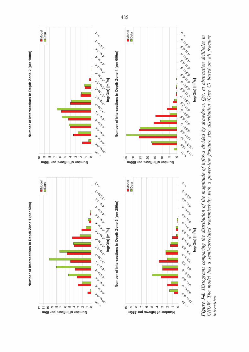
Nu
mb
er o
f in
ters
ecti
on
s in
Dep
th Z
on
e 1
(per
50m
)
0123456789101112
< -1
0 -10
to -9
.5 -9.5
to -9 -9
to -8
.5 -8.5
to -8 -8
to -7
.5 -7.5
to -7 -7
to -6
.5 -6.5
to -6 -6
to -5
.5 -5.5
to -5 -5
to -4
.5 -4.5
to -4 -4
to -3
.5 -3.5
to -3
> -3
log
(Q/s
) [m
2 /s]
Number of inflows per 50mM
odel
Dat
a
Nu
mb
er o
f in
ters
ecti
on
s in
Dep
th Z
on
e 2
(per
100
m)
012345678910
< -1
0 -10
to -9
.5 -9.5
to -9 -9
to -8
.5 -8.5
to -8 -8
to -7
.5 -7.5
to -7 -7
to -6
.5 -6.5
to -6 -6
to -5
.5 -5.5
to -5 -5
to -4
.5 -4.5
to -4 -4
to -3
.5 -3.5
to -3
> -3
log
(Q/s
) [m
2 /s]
Number of inflows per 100m
Mo
del
Da
ta
Nu
mb
er o
f in
ters
ecti
on
s in
Dep
th Z
on
e 3
(per
250
m)
012345678910
< -1
0 -10
to -9
.5 -9.5
to -9 -9
to -8
.5 -8.5
to -8 -8
to -7
.5 -7.5
to -7 -7
to -6
.5 -6.5
to -6 -6
to -5
.5 -5.5
to -5 -5
to -4
.5 -4.5
to -4 -4
to -3
.5 -3.5
to -3
> -3
log
(Q/s
) [m
2 /s]
Number of inflows per 250m
Mo
del
Da
ta
Nu
mb
er o
f in
ters
ecti
on
s in
Dep
th Z
on
e 4
(per
600
m)
05101520253035
< -11
-11
to -1
0.5
-10.
5 to
-10
-10
to -9
.5 -9.5
to -9 -9
to -8
.5 -8.5
to -8 -8
to -7
.5 -7.5
to -7 -7
to -6
.5 -6.5
to -6 -6
to -5
.5 -5.5
to -5 -5
to -4
.5 -4.5
to -4 -4
to -3
.5 -3.5
to -3
> -3
log
(Q/s
) [m
2 /s]
Number of inflows per 600m
Mo
del
Da
ta
Fig
ure
J-8.
His
togr
ams
com
pari
ng th
e di
stri
butio
n of
the
mag
nitu
de o
f inf
low
s di
vide
d by
dra
wdo
wn,
Q/s
, at a
bstr
actio
n dr
illho
les
in
CH
UW
. Th
e m
odel
has
a s
emi-c
orre
late
d tr
ansm
issi
vity
with
a p
ower
-law
fra
ctur
e si
ze d
istr
ibut
ion
(Cas
e C
) ba
sed
on a
ll fr
actu
re
inte
nsiti
es.
485

486
Infl
ow
s in
Dep
th Z
on
e 1
(per
50m
)
-10.
0-9
.0-8
.0-7
.0-6
.0-5
.0-4
.0-3
.0-2
.0-1
.00.
0
PF
L E
-W
Mod
el E
-W
PF
L N
-S
Mod
el N
-S
PF
L S
H
Mod
el S
H
Fracture set
log
(Q
/s)
[m2/s
]
7.8
1.7
5.3
8.2
28.
6
22.
3
Infl
ow
s in
Dep
th Z
on
e 2
(per
100
m)
-10.
0-9
.0-8
.0-7
.0-6
.0-5
.0-4
.0-3
.0-2
.0-1
.00.
0
PF
L E
-W
Mod
el E
-W
PF
L N
-S
Mod
el N
-S
PF
L S
H
Mod
el S
H
Fracture set
log
(Q
/s)
[m2/s
]
4.83.7
3.8 5.8
18.4
16.
9
Infl
ow
s in
Dep
th Z
on
e 3
(per
250
m)
-10.
0-9
.0-8
.0-7
.0-6
.0-5
.0-4
.0-3
.0-2
.0-1
.00.
0
PF
L E
-W
Mod
el E
-W
PF
L N
-S
Mod
el N
-S
PF
L S
H
Mod
el S
H
Fracture set
log
(Q
/s)
[m2/s
]
1.7
2.2
3.2 2.5
12.8
13.0
Infl
ow
s in
Dep
th Z
on
e 4
(per
600
m)
-12.
0-1
1.0
-10.
0-9
.0-8
.0-7
.0-6
.0-5
.0-4
.0-3
.0-2
.0
PF
L E
-W
Mod
el E
-W
PF
L N
-S
Mod
el N
-S
PF
L S
H
Mod
el S
H
Fracture set
log
(Q
/s)
[m2/s
]
31.1
26.
1
24.2
29.
4
43.
8
45.7
Fig
ure
J-9
. Bar
and
whi
sker
plo
ts c
ompa
ring
sta
tist
ics
for
each
frac
ture
set
for
the
indi
vidu
al in
flow
s, Q
/s, f
or th
e P
FL
dat
a fr
om d
rill
hole
se
ctio
ns w
ithi
n C
HU
W a
gain
st s
tati
stic
s fo
r an
ens
embl
e of
40
real
isat
ions
(10
rea
lisa
tion
s pe
r dr
illh
ole)
of
the
Hyd
ro-D
FN
mod
el (
Cas
e C
). T
he n
umbe
rs a
djac
ent t
o ea
ch b
ar a
re th
e Te
rzag
hi w
eigh
ted
num
bers
of s
peci
fic
capa
citi
es a
bove
1.6
10-1
0 m2 /s
.
486

487
Total normalized flow to borehole section (Terzaghi corrected)
-4.9
-5.7
-5.7
-6.7
-4.8
-5.7
-5.7
-6.8
-8.5
-8.0
-7.5
-7.0
-6.5
-6.0
-5.5
-5.0
-4.5
-4.0
-3.5
DZ1 DZ2 DZ3 DZ4
Depth Zone
Lo
g [
Flo
w (
Q/s
)] [
m2 /s
]
Model
Data
Figure J-10. Comparison of the Terzaghi weighted sum of individual specific capacities, Q/s, for the PFL data from drillhole sections within CHUW normalised to the nominal thicknesses of each depth zone, against statistics for an ensemble over 10 realisations of 4 individual drillholes in the Elaborated Hydro-DFN model. The model has a semi-correlated transmissivity with a power-law fracture size distribution (Case C) based on all fracture intensities. For the data, statistics are taken over the identified flowing fractures within each set. For the model, statistics are generated over 40 realisations. The total flows are normalised to the following lengths: Depth Zone 1 is 50 m, Depth Zone 2 is 100 m, Depth Zone 3 is 250 m, and Depth Zone 4 is 600 m.

488
Case A
Table J-2. Summary of Elaborated Hydro-DFN parameters for the simulations of flow in hydraulic domain CHUW, using a power-law size model (Case A).
Set Distribution of poles
Pole orientation F: trend, plunge, conc. B: (trend, plunge), conc.1, conc.2, rot.
Case A power-law (kr, r0) rmin = r0
rmax = 564 m
Intensity P32,open
Transmissivity model C: (a,b) SC: (a, b, σlog(T)) UC: (µ log(T), σ log(T))
(-, m) (m2/m3) T (m2s-1)
Depth Zone 1
EW Fisher (176.0, 4.4), 9.4 (2.68, 0.04) 0.49 C: (3.0E-8, 0.8) SC: (8.0E-8, 0.4, 0.6) UC: (2.0E-7, 0.6)
NS Fisher (270.4, 0.2), 8.3 (2.57, 0.04) 0.57 C: (3.0E-8, 0.7) SC: (6.0E-8, 0.6, 0.6) UC: (8.0E-8, 0.8)
SH Bingham (300.1, 78.9)
-5.7, -4.4, 50.6o (2.53, 0.04) 2.09
C: (7.0E-8, 0.9) SC: (1.2E-7, 0.7, 0.8) UC: (7.0E-7, 1.1)
Depth Zone 2
EW Fisher (176.0, 4.4), 9.4 (2.58, 0.04) 0.21 C: (8.0E-9, 0.8) SC: (9.0E-9, 0.6, 0.4) UC: (2.0E-8, 1.1)
NS Fisher (270.4, 0.2), 8.3 (2.52, 0.04) 0.25 C: (1.5E-8, 0.8) SC: (1.0E-8, 0.6, 0.6) UC: (4.0E-8, 0.9)
SH Bingham (300.1, 78.9)
-5.7, -4.4, 50.6o (2.45, 0.04) 0.91
C: (1.2E-8,0.8) SC: (1.0E-8, 0.6, 0.6) UC: (6.0E-8, 0.8)
Depth Zone 3
EW Fisher (176.0, 4.4), 9.4 (2.50, 0.04) 0.11 C: (2.2E-9, 0.7) SC: (4.0E-9, 0.7, 0.6) UC: (1.0E-8, 0.8)
NS Fisher (270.4, 0.2), 8.3 (2.65, 0.04) 0.13 C: (6.0E-9, 0.6) SC: (1.0E-8, 0.2, 0.2) UC: (1.7E-8, 0.4)
SH Bingham (300.1, 78.9)
-5.7, -4.4, 50.6o (2.35, 0.04) 0.34
C: (2.0E-9, 1.2) SC: (1.0E-9, 1.0, 1.0) UC: (6.0E-8, 1.1)
Depth Zone 4
EW Fisher (176.0, 4.4), 9.4 (2.40, 0.60) 0.07 C: (7.0E-11, 0.7) SC: (5.0E-11, 0.8, 0.2)UC: (3.0E-10, 0.5)
NS Fisher (270.4, 0.2), 8.3 (2.40, 0.60) 0.08 C: (8.0E-11, 0.9) SC: (6.0E-11, 0.7, 0.5)UC: (5.0E-10, 0.8)
SH Bingham (300.1, 78.9)
-5.7, -4.4, 50.6o (2.40, 0.60) 0.17
C: (6.0E-11, 1.0) SC: (5.0E-11, 1.0, 0.6)UC: (1.0E-9, 0.9)
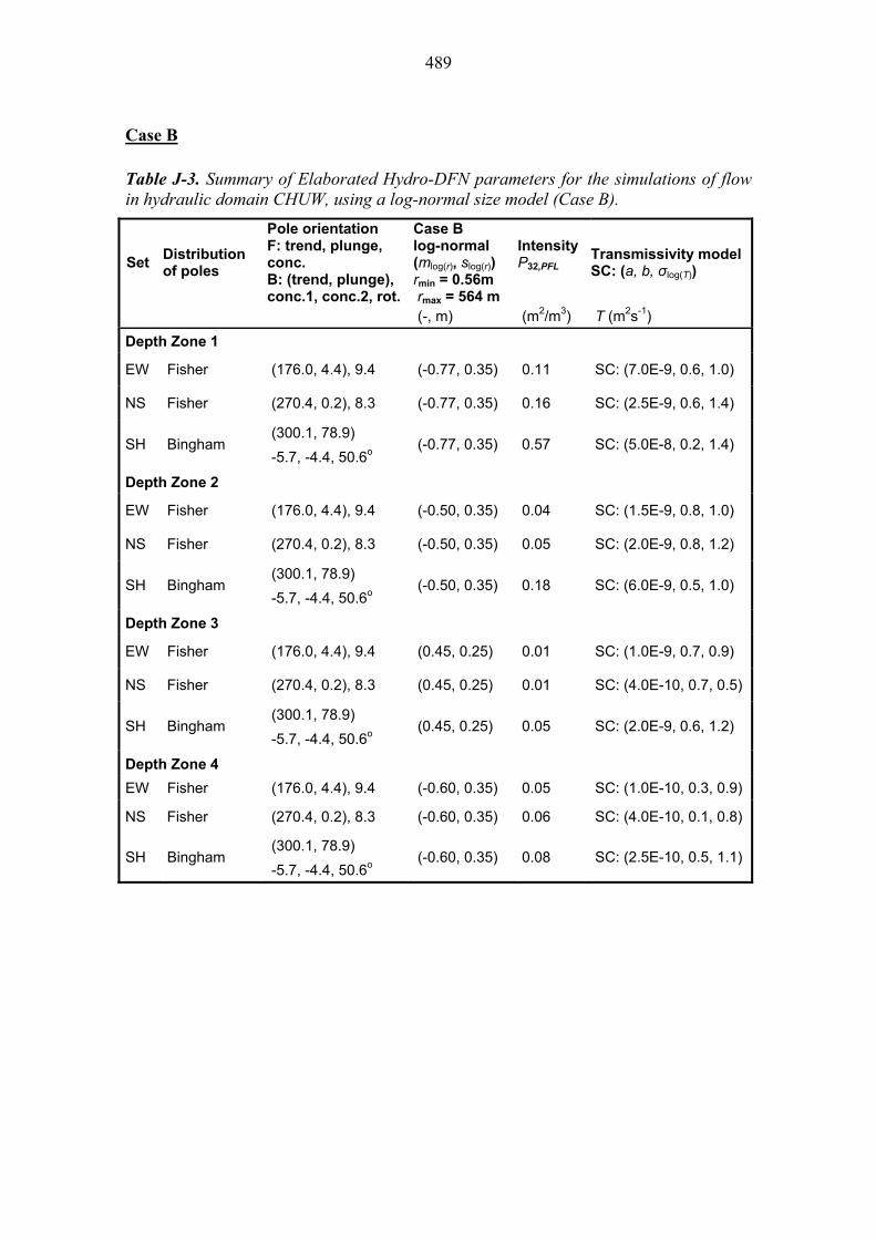
489
Case B
Table J-3. Summary of Elaborated Hydro-DFN parameters for the simulations of flow in hydraulic domain CHUW, using a log-normal size model (Case B).
Set Distribution of poles
Pole orientation F: trend, plunge, conc. B: (trend, plunge), conc.1, conc.2, rot.
Case B log-normal (mlog(r), slog(r)) rmin = 0.56m rmax = 564 m
Intensity P32,PFL
Transmissivity model SC: (a, b, σlog(T))
(-, m) (m2/m3) T (m2s-1)
Depth Zone 1
EW Fisher (176.0, 4.4), 9.4 (-0.77, 0.35) 0.11 SC: (7.0E-9, 0.6, 1.0)
NS Fisher (270.4, 0.2), 8.3 (-0.77, 0.35) 0.16 SC: (2.5E-9, 0.6, 1.4)
SH Bingham (300.1, 78.9)
-5.7, -4.4, 50.6o (-0.77, 0.35) 0.57 SC: (5.0E-8, 0.2, 1.4)
Depth Zone 2
EW Fisher (176.0, 4.4), 9.4 (-0.50, 0.35) 0.04 SC: (1.5E-9, 0.8, 1.0)
NS Fisher (270.4, 0.2), 8.3 (-0.50, 0.35) 0.05 SC: (2.0E-9, 0.8, 1.2)
SH Bingham (300.1, 78.9)
-5.7, -4.4, 50.6o (-0.50, 0.35) 0.18 SC: (6.0E-9, 0.5, 1.0)
Depth Zone 3
EW Fisher (176.0, 4.4), 9.4 (0.45, 0.25) 0.01 SC: (1.0E-9, 0.7, 0.9)
NS Fisher (270.4, 0.2), 8.3 (0.45, 0.25) 0.01 SC: (4.0E-10, 0.7, 0.5)
SH Bingham (300.1, 78.9)
-5.7, -4.4, 50.6o (0.45, 0.25) 0.05 SC: (2.0E-9, 0.6, 1.2)
Depth Zone 4
EW Fisher (176.0, 4.4), 9.4 (-0.60, 0.35) 0.05 SC: (1.0E-10, 0.3, 0.9)
NS Fisher (270.4, 0.2), 8.3 (-0.60, 0.35) 0.06 SC: (4.0E-10, 0.1, 0.8)
SH Bingham (300.1, 78.9)
-5.7, -4.4, 50.6o (-0.60, 0.35) 0.08 SC: (2.5E-10, 0.5, 1.1)

490
Case C
Table J-4. Summary of Elaborated Hydro-DFN parameters for the simulations of flow in hydraulic domain CHUW, using a power-law size model (r0=0.2, kr=2.59) with channels (Case C).
Set Distribution of poles
Pole orientation F: trend, plunge, conc. B: (trend, plunge), conc. 1, conc.2, rot.
Case C deletion parameters (d, a)
Intensity P32,open
Transmissivity model SC: (a, b, σlog(T))
(-, m) (m2/m3) T (m2s-1)
Depth Zone 1
EW Fisher (176.0, 4.4), 9.4 (16.00, 1.90) 0.89 SC: (6.0E-8, 0.35, 0.9)
NS Fisher (270.4, 0.2), 8.3 (25.00, 6.35) 1.04 SC: (1.5E-8, 0.5, 1.0)
SH Bingham (300.1, 78.9)
-5.7, -4.4, 50.6o (19.25, 3.51) 3.79 SC: (8.0E-8, 0.6, 0.9)
Depth Zone 2
EW Fisher (176.0, 4.4), 9.4 (13.60, 0.72) 0.54 SC: (5.0E-9, 0.55, 1.0)
NS Fisher (270.4, 0.2), 8.3 (14.00, 0.92) 0.63 SC: (7.0E-9, 0.45, 1.1)
SH Bingham (300.1, 78.9)
-5.7, -4.4, 50.6o (15.25, 1.53) 2.28 SC: (1.1E-8, 0.45, 0.9)
Depth Zone 3
EW Fisher (176.0, 4.4), 9.4 (9.75, -1.18) 0.51 SC: (1.5E-9, 0.7, 0.5)
NS Fisher (270.4, 0.2), 8.3 (6.15, -2.96) 0.64 SC: (3.0E-9, 0.5, 0.5)
SH Bingham (300.1, 78.9)
-5.7, -4.4, 50.6o (11.40, -0.37) 1.61 SC: (2.5E-9, 1.0, 1.2)
Depth Zone 4
EW Fisher (176.0, 4.4), 9.4 (35.00, 11.29) 0.39 SC: (1.0E-10, 0.65, 0.3)
NS Fisher (270.4, 0.2), 8.3 (100.00, 43.40)
0.46 SC: (1.0E-10, 0.65, 0.6)
SH Bingham (300.1, 78.9)
-5.7, -4.4, 50.6o (22.00, 4.87) 0.93 SC: (2.5E-10, 1.0, 0.6)
491
APPENDIX K: PALAEOHYDROGEOLOGICAL UNCERTAINTIES
Stochastic uncertainties for site-scale palaeohydrogeological simulations are examined in section 13.5 for five realisations of the Case A semi-correlated model. This appendix details equivalent analysis of groundwater composition and head for individual drillholes based on two realisations of:
the Case A correlated model,
the Case A uncorrelated model,
the Case B semi-correlated model,
the Case C semi-correlated model.
Predictions of groundwater head values are presented in section K.1 and compared to observations. Concentrations of SO4 and HCO3 are compared with measured values in sections K.2 and K.3 respectively.
K.1 Groundwater head predictions
Comparisons of measured groundwater head with predictions from two realisations of the Case A correlated and uncorrelated model, along with two realisations of the semi-correlated Case B and Case C models are detailed below. For each model case, results are presented on an individual drillhole basis for KR1 through KR15 in Figure K-1 to Figure K-8. Minimal variation in groundwater head occurs between realisations, with profiles accurately representing measurements in most drillholes.
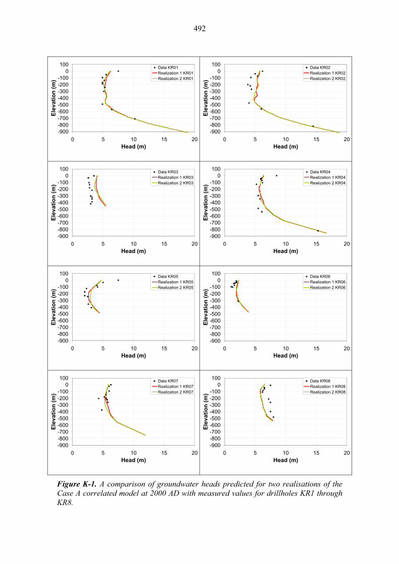
492
-900-800-700-600-500-400-300-200-100
0100
0 5 10 15 20Head (m)
Ele
vati
on
(m
)
Data KR01Realization 1 KR01Realization 2 KR01
-900-800-700-600-500-400-300-200-100
0100
0 5 10 15 20Head (m)
Ele
vati
on
(m
)
Data KR02Realization 1 KR02Realization 2 KR02
-900-800-700-600-500-400-300-200-100
0100
0 5 10 15 20Head (m)
Ele
vati
on
(m
)
Data KR03Realization 1 KR03Realization 2 KR03
-900-800-700-600-500-400-300-200-100
0100
0 5 10 15 20Head (m)
Ele
vati
on
(m
)
Data KR04Realization 1 KR04Realization 2 KR04
-900-800-700-600-500-400-300-200-100
0100
0 5 10 15 20Head (m)
Ele
vati
on
(m
)
Data KR05Realization 1 KR05Realization 2 KR05
-900-800-700-600-500-400-300-200-100
0100
0 5 10 15 20Head (m)
Ele
vat
ion
(m
)
Data KR06Realization 1 KR06Realization 2 KR06
-900-800-700-600-500-400-300-200-100
0100
0 5 10 15 20Head (m)
Ele
vati
on
(m
)
Data KR07Realization 1 KR07Realization 2 KR07
-900-800-700-600-500-400-300-200-100
0100
0 5 10 15 20Head (m)
Ele
vati
on
(m
)
Data KR08Realization 1 KR08Realization 2 KR08
Figure K-1. A comparison of groundwater heads predicted for two realisations of the Case A correlated model at 2000 AD with measured values for drillholes KR1 through KR8.
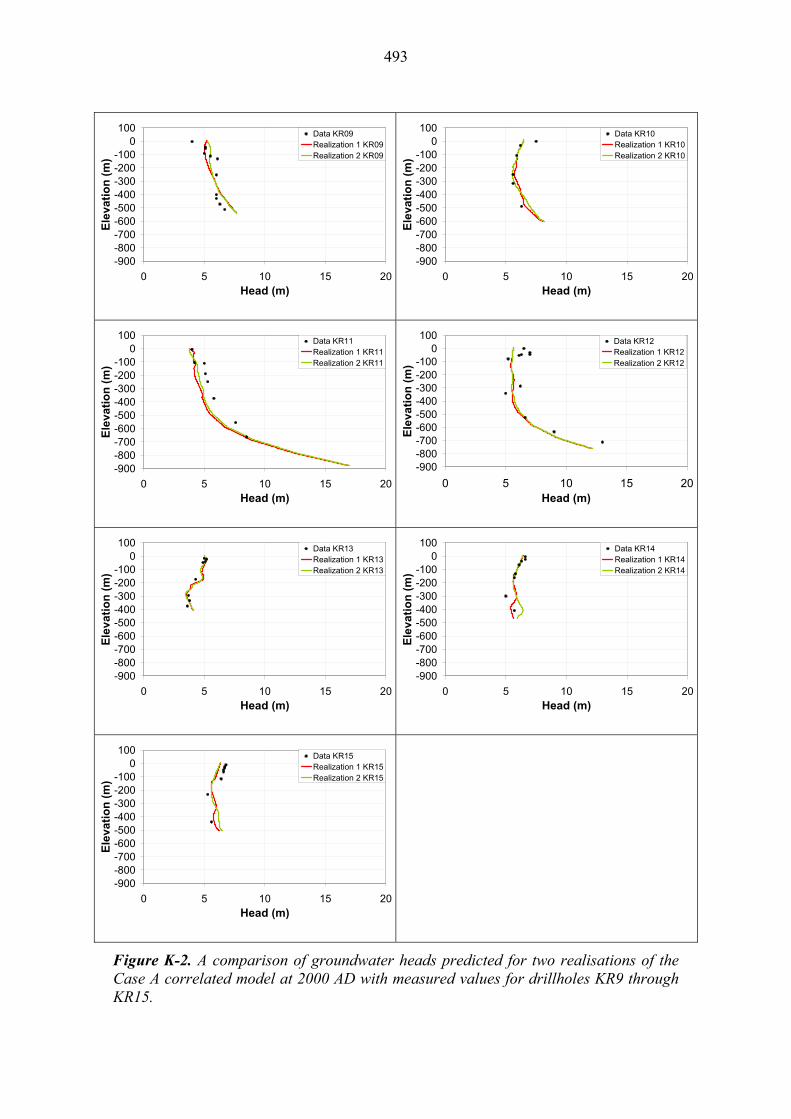
493
-900-800-700-600-500-400-300-200-100
0100
0 5 10 15 20Head (m)
Ele
vati
on
(m
)
Data KR09Realization 1 KR09Realization 2 KR09
-900-800-700-600-500-400-300-200-100
0100
0 5 10 15 20Head (m)
Ele
vati
on
(m
)
Data KR10Realization 1 KR10Realization 2 KR10
-900-800-700-600-500-400-300-200-100
0100
0 5 10 15 20Head (m)
Ele
vati
on
(m
)
Data KR11Realization 1 KR11Realization 2 KR11
-900-800-700-600-500-400-300-200-100
0100
0 5 10 15 20Head (m)
Ele
vati
on
(m
)
Data KR12Realization 1 KR12Realization 2 KR12
-900-800-700-600-500-400-300-200-100
0100
0 5 10 15 20Head (m)
Ele
vati
on
(m
)
Data KR13Realization 1 KR13Realization 2 KR13
-900-800-700-600-500-400-300-200-100
0100
0 5 10 15 20Head (m)
Ele
vati
on
(m
)
Data KR14Realization 1 KR14Realization 2 KR14
-900-800-700-600-500-400-300-200-100
0100
0 5 10 15 20Head (m)
Ele
vati
on
(m
)
Data KR15Realization 1 KR15Realization 2 KR15
Figure K-2. A comparison of groundwater heads predicted for two realisations of the Case A correlated model at 2000 AD with measured values for drillholes KR9 through KR15.

494
-900-800-700-600-500-400-300-200-100
0100
0 5 10 15 20Head (m)
Ele
vati
on
(m
)
Data KR01Realization 1 KR01Realization 2 KR01
-900-800-700-600-500-400-300-200-100
0100
0 5 10 15 20Head (m)
Ele
vati
on
(m
)
Data KR02Realization 1 KR02Realization 2 KR02
-900-800-700-600-500-400-300-200-100
0100
0 5 10 15 20Head (m)
Ele
vati
on
(m
)
Data KR03Realization 1 KR03Realization 2 KR03
-900-800-700-600-500-400-300-200-100
0100
0 5 10 15 20Head (m)
Ele
vati
on
(m
)
Data KR04Realization 1 KR04Realization 2 KR04
-900-800-700-600-500-400-300-200-100
0100
0 5 10 15 20Head (m)
Ele
vati
on
(m
)
Data KR05Realization 1 KR05Realization 2 KR05
-900-800-700-600-500-400-300-200-100
0100
0 5 10 15 20Head (m)
Ele
vat
ion
(m
)
Data KR06Realization 1 KR06Realization 2 KR06
-900-800-700-600-500-400-300-200-100
0100
0 5 10 15 20Head (m)
Ele
vati
on
(m
)
Data KR07Realization 1 KR07Realization 2 KR07
-900-800-700-600-500-400-300-200-100
0100
0 5 10 15 20Head (m)
Ele
vati
on
(m
)
Data KR08Realization 1 KR08Realization 2 KR08
Figure K-3. A comparison of groundwater heads predicted for two realisations of the Case A uncorrelated model at 2000 AD with measured values for drillholes KR1 through KR8.
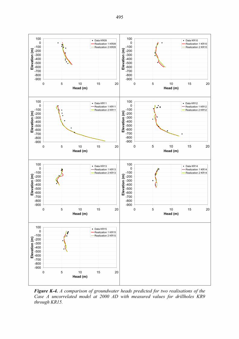
495
-900-800-700-600-500-400-300-200-100
0100
0 5 10 15 20Head (m)
Ele
vati
on
(m
)
Data KR09Realization 1 KR09Realization 2 KR09
-900-800-700-600-500-400-300-200-100
0100
0 5 10 15 20Head (m)
Ele
vati
on
(m
)
Data KR10Realization 1 KR10Realization 2 KR10
-900-800-700-600-500-400-300-200-100
0100
0 5 10 15 20Head (m)
Ele
vati
on
(m
)
Data KR11Realization 1 KR11Realization 2 KR11
-900-800-700-600-500-400-300-200-100
0100
0 5 10 15 20Head (m)
Ele
vati
on
(m
)
Data KR12Realization 1 KR12Realization 2 KR12
-900-800-700-600-500-400-300-200-100
0100
0 5 10 15 20Head (m)
Ele
vati
on
(m
)
Data KR13Realization 1 KR13Realization 2 KR13
-900-800-700-600-500-400-300-200-100
0100
0 5 10 15 20Head (m)
Ele
vati
on
(m
)
Data KR14Realization 1 KR14Realization 2 KR14
-900-800-700-600-500-400-300-200-100
0100
0 5 10 15 20Head (m)
Ele
vati
on
(m
)
Data KR15Realization 1 KR15Realization 2 KR15
Figure K-4. A comparison of groundwater heads predicted for two realisations of the Case A uncorrelated model at 2000 AD with measured values for drillholes KR9 through KR15.

496
-900-800-700-600-500-400-300-200-100
0100
0 5 10 15 20Head (m)
Ele
vati
on
(m
)
Data KR01Realization 1 KR01Realization 2 KR01
-900-800-700-600-500-400-300-200-100
0100
0 5 10 15 20Head (m)
Ele
vati
on
(m
)
Data KR02Realization 1 KR02Realization 2 KR02
-900-800-700-600-500-400-300-200-100
0100
0 5 10 15 20Head (m)
Ele
vati
on
(m
)
Data KR03Realization 1 KR03Realization 2 KR03
-900-800-700-600-500-400-300-200-100
0100
0 5 10 15 20Head (m)
Ele
vati
on
(m
)
Data KR04Realization 1 KR04Realization 2 KR04
-900-800-700-600-500-400-300-200-100
0100
0 5 10 15 20Head (m)
Ele
vati
on
(m
)
Data KR05Realization 1 KR05Realization 2 KR05
-900-800-700-600-500-400-300-200-100
0100
0 5 10 15 20Head (m)
Ele
vat
ion
(m
)
Data KR06Realization 1 KR06Realization 2 KR06
-900-800-700-600-500-400-300-200-100
0100
0 5 10 15 20Head (m)
Ele
vati
on
(m
)
Data KR07Realization 1 KR07Realization 2 KR07
-900-800-700-600-500-400-300-200-100
0100
0 5 10 15 20Head (m)
Ele
vati
on
(m
)
Data KR08Realization 1 KR08Realization 2 KR08
Figure K-5. A comparison of groundwater heads predicted for two realisations of the Case B semi-correlated model at 2000 AD with measured values for drillholes KR1 through KR8.

497
-900-800-700-600-500-400-300-200-100
0100
0 5 10 15 20Head (m)
Ele
vati
on
(m
)
Data KR09Realization 1 KR09Realization 2 KR09
-900-800-700-600-500-400-300-200-100
0100
0 5 10 15 20Head (m)
Ele
vati
on
(m
)
Data KR10Realization 1 KR10Realization 2 KR10
-900-800-700-600-500-400-300-200-100
0100
0 5 10 15 20Head (m)
Ele
vati
on
(m
)
Data KR11Realization 1 KR11Realization 2 KR11
-900-800-700-600-500-400-300-200-100
0100
0 5 10 15 20Head (m)
Ele
vati
on
(m
)
Data KR12Realization 1 KR12Realization 2 KR12
-900-800-700-600-500-400-300-200-100
0100
0 5 10 15 20Head (m)
Ele
vati
on
(m
)
Data KR13Realization 1 KR13Realization 2 KR13
-900-800-700-600-500-400-300-200-100
0100
0 5 10 15 20Head (m)
Ele
vati
on
(m
)
Data KR14Realization 1 KR14Realization 2 KR14
-900-800-700-600-500-400-300-200-100
0100
0 5 10 15 20Head (m)
Ele
vati
on
(m
)
Data KR15Realization 1 KR15Realization 2 KR15
Figure K-6. A comparison of groundwater heads predicted for two realisations of the Case B semi-correlated model at 2000 AD with measured values for drillholes KR9 through KR15.
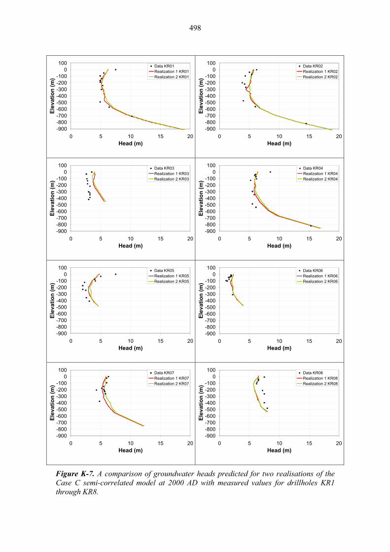
498
-900-800-700-600-500-400-300-200-100
0100
0 5 10 15 20Head (m)
Ele
vati
on
(m
)
Data KR01Realization 1 KR01Realization 2 KR01
-900-800-700-600-500-400-300-200-100
0100
0 5 10 15 20Head (m)
Ele
vati
on
(m
)
Data KR02Realization 1 KR02Realization 2 KR02
-900-800-700-600-500-400-300-200-100
0100
0 5 10 15 20Head (m)
Ele
vati
on
(m
)
Data KR03Realization 1 KR03Realization 2 KR03
-900-800-700-600-500-400-300-200-100
0100
0 5 10 15 20Head (m)
Ele
vati
on
(m
)
Data KR04Realization 1 KR04Realization 2 KR04
-900-800-700-600-500-400-300-200-100
0100
0 5 10 15 20Head (m)
Ele
vati
on
(m
)
Data KR05Realization 1 KR05Realization 2 KR05
-900-800-700-600-500-400-300-200-100
0100
0 5 10 15 20Head (m)
Ele
vat
ion
(m
)
Data KR06Realization 1 KR06Realization 2 KR06
-900-800-700-600-500-400-300-200-100
0100
0 5 10 15 20Head (m)
Ele
vati
on
(m
)
Data KR07Realization 1 KR07Realization 2 KR07
-900-800-700-600-500-400-300-200-100
0100
0 5 10 15 20Head (m)
Ele
vati
on
(m
)
Data KR08Realization 1 KR08Realization 2 KR08
Figure K-7. A comparison of groundwater heads predicted for two realisations of the Case C semi-correlated model at 2000 AD with measured values for drillholes KR1 through KR8.
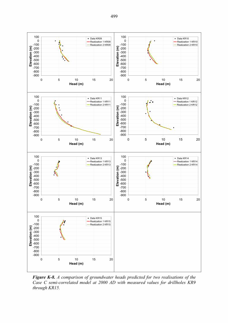
499
-900-800-700-600-500-400-300-200-100
0100
0 5 10 15 20Head (m)
Ele
vati
on
(m
)
Data KR09Realization 1 KR09Realization 2 KR09
-900-800-700-600-500-400-300-200-100
0100
0 5 10 15 20Head (m)
Ele
vati
on
(m
)
Data KR10Realization 1 KR10Realization 2 KR10
-900-800-700-600-500-400-300-200-100
0100
0 5 10 15 20Head (m)
Ele
vati
on
(m
)
Data KR11Realization 1 KR11Realization 2 KR11
-900-800-700-600-500-400-300-200-100
0100
0 5 10 15 20Head (m)
Ele
vati
on
(m
)
Data KR12Realization 1 KR12Realization 2 KR12
-900-800-700-600-500-400-300-200-100
0100
0 5 10 15 20Head (m)
Ele
vati
on
(m
)
Data KR13Realization 1 KR13Realization 2 KR13
-900-800-700-600-500-400-300-200-100
0100
0 5 10 15 20Head (m)
Ele
vati
on
(m
)
Data KR14Realization 1 KR14Realization 2 KR14
-900-800-700-600-500-400-300-200-100
0100
0 5 10 15 20Head (m)
Ele
vati
on
(m
)
Data KR15Realization 1 KR15Realization 2 KR15
Figure K-8. A comparison of groundwater heads predicted for two realisations of the Case C semi-correlated model at 2000 AD with measured values for drillholes KR9 through KR15.

500
K.2 Groundwater concentrations of sulphate
Comparisons of measured SO4 concentrations in groundwater with predictions from two realisations of the Case A correlated and uncorrelated model, along with two realisations of the semi-correlated Case B and Case C models are detailed below. For each model case, results are presented on an individual drillhole basis for KR1 through KR15 in Figure K-9 to Figure K-16. Greater variations in sulphate concentration with depth occur between model realisations than for the corresponding groundwater head analysis in section K.1. From just two simulations, a number of measured SO4 concentrations become realizable, and it is expected that if additional realisations were considered, a greater proportion of the concentrations observed would be captured within the envelope of results.

501
-900-800-700-600-500-400-300-200-100
0100
0 100 200 300 400 500 600SO4 (mg/L)
Ele
vati
on
(m
)
Data KR01Realization 1 KR01Realization 2 KR01
-900-800-700-600-500-400-300-200-100
0100
0 100 200 300 400 500 600SO4 (mg/L)
Ele
vati
on
(m
)
Data KR02Realization 1 KR02Realization 2 KR02
-900-800-700-600-500-400-300-200-100
0100
0 100 200 300 400 500 600SO4 (mg/L)
Ele
vati
on
(m
)
Data KR03Realization 1 KR03Realization 2 KR03
-900-800-700-600-500-400-300-200-100
0100
0 100 200 300 400 500 600SO4 (mg/L)
Ele
vati
on
(m
)
Data KR04Realization 1 KR04Realization 2 KR04
-900-800-700-600-500-400-300-200-100
0100
0 100 200 300 400 500 600SO4 (mg/L)
Ele
vati
on
(m
)
Data KR05Realization 1 KR05Realization 2 KR05 -900
-800-700-600-500-400-300-200-100
0100
0 100 200 300 400 500 600SO4 (mg/L)
Ele
vati
on
(m
)
Data KR06Realization 1 KR06Realization 2 KR06
-900-800-700-600-500-400-300-200-100
0100
0 100 200 300 400 500 600SO4 (mg/L)
Ele
vati
on
(m
)
Data KR07Realization 1 KR07Realization 2 KR07
-900-800-700-600-500-400-300-200-100
0100
0 100 200 300 400 500 600SO4 (mg/L)
Ele
vati
on
(m
)
Data KR08Realization 1 KR08Realization 2 KR08
Figure K-9. A comparison of SO4 concentrations predicted from two realisations of the Case A correlated model at 2000 AD with measured values for drillholes KR1 through KR8.

502
-900-800-700-600-500-400-300-200-100
0100
0 100 200 300 400 500 600SO4 (mg/L)
Ele
vati
on
(m
)
Data KR09Realization 1 KR09Realization 2 KR09
-900-800-700-600-500-400-300-200-100
0100
0 100 200 300 400 500 600SO4 (mg/L)
Ele
vati
on
(m
)
Data KR10Realization 1 KR10Realization 2 KR10
-900-800-700-600-500-400-300-200-100
0100
0 100 200 300 400 500 600SO4 (mg/L)
Ele
vati
on
(m
)
Data KR11Realization 1 KR11Realization 2 KR11
-900-800-700-600-500-400-300-200-100
0100
0 100 200 300 400 500 600SO4 (mg/L)
Ele
vati
on
(m
)
Data KR12Realization 1 KR12Realization 2 KR12
-900-800-700-600-500-400-300-200-100
0100
0 100 200 300 400 500 600SO4 (mg/L)
Ele
vati
on
(m
)
Data KR13Realization 1 KR13Realization 2 KR13 -900
-800-700-600-500-400-300-200-100
0100
0 100 200 300 400 500 600SO4 (mg/L)
Ele
vati
on
(m
)
Data KR14Realization 1 KR14Realization 2 KR14
-900-800-700-600-500-400-300-200-100
0100
0 100 200 300 400 500 600SO4 (mg/L)
Ele
vati
on
(m
)
Data KR15Realization 1 KR15Realization 2 KR15
Figure K-10. A comparison of SO4 concentrations predicted from two realisations of the Case A correlated model at 2000 AD with measured values for drillholes KR9 through KR15.

503
-900-800-700-600-500-400-300-200-100
0100
0 100 200 300 400 500 600SO4 (mg/L)
Ele
vati
on
(m
)
Data KR01Realization 1 KR01Realization 2 KR01
-900-800-700-600-500-400-300-200-100
0100
0 100 200 300 400 500 600SO4 (mg/L)
Ele
vati
on
(m
)
Data KR02Realization 1 KR02Realization 2 KR02
-900-800-700-600-500-400-300-200-100
0100
0 100 200 300 400 500 600SO4 (mg/L)
Ele
vati
on
(m
)
Data KR03Realization 1 KR03Realization 2 KR03
-900-800-700-600-500-400-300-200-100
0100
0 100 200 300 400 500 600SO4 (mg/L)
Ele
vati
on
(m
)
Data KR04Realization 1 KR04Realization 2 KR04
-900-800-700-600-500-400-300-200-100
0100
0 100 200 300 400 500 600SO4 (mg/L)
Ele
vati
on
(m
)
Data KR05Realization 1 KR05Realization 2 KR05 -900
-800-700-600-500-400-300-200-100
0100
0 100 200 300 400 500 600SO4 (mg/L)
Ele
vati
on
(m
)
Data KR06Realization 1 KR06Realization 2 KR06
-900-800-700-600-500-400-300-200-100
0100
0 100 200 300 400 500 600SO4 (mg/L)
Ele
vati
on
(m
)
Data KR07Realization 1 KR07Realization 2 KR07
-900-800-700-600-500-400-300-200-100
0100
0 100 200 300 400 500 600SO4 (mg/L)
Ele
vati
on
(m
)
Data KR08Realization 1 KR08Realization 2 KR08
Figure K-11. A comparison of SO4 concentrations predicted from two realisations of the Case A uncorrelated model at 2000 AD with measured values for drillholes KR1 through KR8.
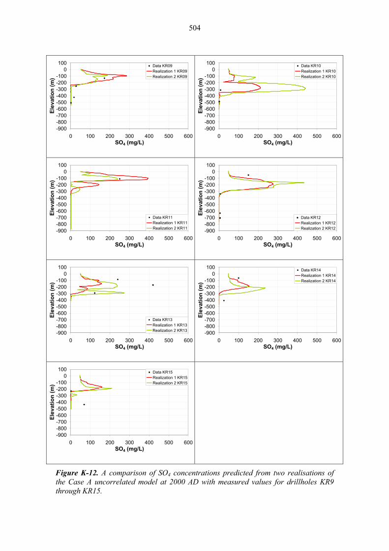
504
-900-800-700-600-500-400-300-200-100
0100
0 100 200 300 400 500 600SO4 (mg/L)
Ele
vati
on
(m
)
Data KR09Realization 1 KR09Realization 2 KR09
-900-800-700-600-500-400-300-200-100
0100
0 100 200 300 400 500 600SO4 (mg/L)
Ele
vati
on
(m
)
Data KR10Realization 1 KR10Realization 2 KR10
-900-800-700-600-500-400-300-200-100
0100
0 100 200 300 400 500 600SO4 (mg/L)
Ele
vati
on
(m
)
Data KR11Realization 1 KR11Realization 2 KR11 -900
-800-700-600-500-400-300-200-100
0100
0 100 200 300 400 500 600SO4 (mg/L)
Ele
vati
on
(m
)
Data KR12Realization 1 KR12Realization 2 KR12
-900-800-700-600-500-400-300-200-100
0100
0 100 200 300 400 500 600SO4 (mg/L)
Ele
vati
on
(m
)
Data KR13Realization 1 KR13Realization 2 KR13 -900
-800-700-600-500-400-300-200-100
0100
0 100 200 300 400 500 600SO4 (mg/L)
Ele
vati
on
(m
)
Data KR14Realization 1 KR14Realization 2 KR14
-900-800-700-600-500-400-300-200-100
0100
0 100 200 300 400 500 600SO4 (mg/L)
Ele
vati
on
(m
)
Data KR15Realization 1 KR15Realization 2 KR15
Figure K-12. A comparison of SO4 concentrations predicted from two realisations of the Case A uncorrelated model at 2000 AD with measured values for drillholes KR9 through KR15.

505
-900-800-700-600-500-400-300-200-100
0100
0 100 200 300 400 500 600SO4 (mg/L)
Ele
vati
on
(m
)
Data KR01Realization 1 KR01Realization 2 KR01
-900-800-700-600-500-400-300-200-100
0100
0 100 200 300 400 500 600SO4 (mg/L)
Ele
vati
on
(m
)
Data KR02Realization 1 KR02Realization 2 KR02
-900-800-700-600-500-400-300-200-100
0100
0 100 200 300 400 500 600SO4 (mg/L)
Ele
vati
on
(m
)
Data KR03Realization 1 KR03Realization 2 KR03
-900-800-700-600-500-400-300-200-100
0100
0 100 200 300 400 500 600SO4 (mg/L)
Ele
vati
on
(m
)
Data KR04Realization 1 KR04Realization 2 KR04
-900-800-700-600-500-400-300-200-100
0100
0 100 200 300 400 500 600SO4 (mg/L)
Ele
vati
on
(m
)
Data KR05Realization 1 KR05Realization 2 KR05 -900
-800-700-600-500-400-300-200-100
0100
0 100 200 300 400 500 600SO4 (mg/L)
Ele
vati
on
(m
)
Data KR06Realization 1 KR06Realization 2 KR06
-900-800-700-600-500-400-300-200-100
0100
0 100 200 300 400 500 600SO4 (mg/L)
Ele
vati
on
(m
)
Data KR07Realization 1 KR07Realization 2 KR07
-900-800-700-600-500-400-300-200-100
0100
0 100 200 300 400 500 600SO4 (mg/L)
Ele
vati
on
(m
)
Data KR08Realization 1 KR08Realization 2 KR08
Figure K-13. A comparison of the SO4 concentrations predicted from two realisations of the Case B semi-correlated model at 2000 AD with measured values for drillholes KR1 through KR8.
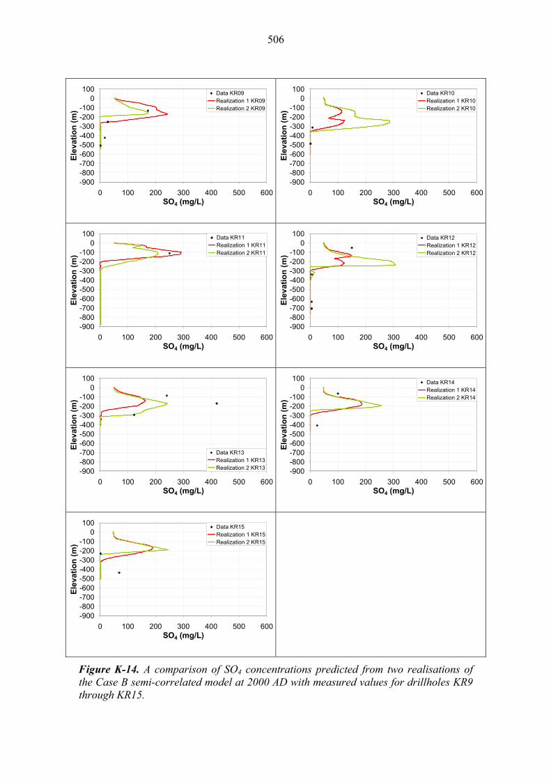
506
-900-800-700-600-500-400-300-200-100
0100
0 100 200 300 400 500 600SO4 (mg/L)
Ele
vati
on
(m
)
Data KR09Realization 1 KR09Realization 2 KR09
-900-800-700-600-500-400-300-200-100
0100
0 100 200 300 400 500 600SO4 (mg/L)
Ele
vati
on
(m
)
Data KR10Realization 1 KR10Realization 2 KR10
-900-800-700-600-500-400-300-200-100
0100
0 100 200 300 400 500 600SO4 (mg/L)
Ele
vati
on
(m
)
Data KR11Realization 1 KR11Realization 2 KR11
-900-800-700-600-500-400-300-200-100
0100
0 100 200 300 400 500 600SO4 (mg/L)
Ele
vati
on
(m
)
Data KR12Realization 1 KR12Realization 2 KR12
-900-800-700-600-500-400-300-200-100
0100
0 100 200 300 400 500 600SO4 (mg/L)
Ele
vati
on
(m
)
Data KR13Realization 1 KR13Realization 2 KR13 -900
-800-700-600-500-400-300-200-100
0100
0 100 200 300 400 500 600SO4 (mg/L)
Ele
vati
on
(m
)
Data KR14Realization 1 KR14Realization 2 KR14
-900-800-700-600-500-400-300-200-100
0100
0 100 200 300 400 500 600SO4 (mg/L)
Ele
vati
on
(m
)
Data KR15Realization 1 KR15Realization 2 KR15
Figure K-14. A comparison of SO4 concentrations predicted from two realisations of the Case B semi-correlated model at 2000 AD with measured values for drillholes KR9 through KR15.
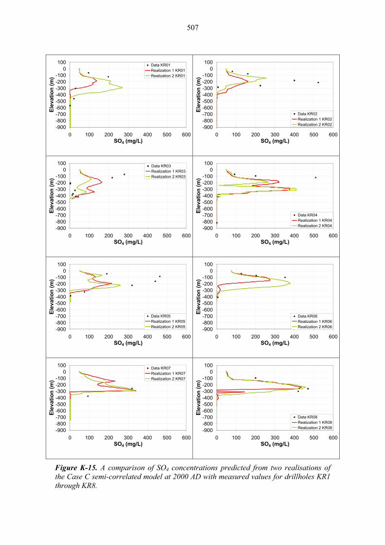
507
-900-800-700-600-500-400-300-200-100
0100
0 100 200 300 400 500 600SO4 (mg/L)
Ele
vati
on
(m
)
Data KR01Realization 1 KR01Realization 2 KR01
-900-800-700-600-500-400-300-200-100
0100
0 100 200 300 400 500 600SO4 (mg/L)
Ele
vati
on
(m
)
Data KR02Realization 1 KR02Realization 2 KR02
-900-800-700-600-500-400-300-200-100
0100
0 100 200 300 400 500 600SO4 (mg/L)
Ele
vati
on
(m
)
Data KR03Realization 1 KR03Realization 2 KR03
-900-800-700-600-500-400-300-200-100
0100
0 100 200 300 400 500 600SO4 (mg/L)
Ele
vati
on
(m
)
Data KR04Realization 1 KR04Realization 2 KR04
-900-800-700-600-500-400-300-200-100
0100
0 100 200 300 400 500 600SO4 (mg/L)
Ele
vati
on
(m
)
Data KR05Realization 1 KR05Realization 2 KR05 -900
-800-700-600-500-400-300-200-100
0100
0 100 200 300 400 500 600SO4 (mg/L)
Ele
vati
on
(m
)
Data KR06Realization 1 KR06Realization 2 KR06
-900-800-700-600-500-400-300-200-100
0100
0 100 200 300 400 500 600SO4 (mg/L)
Ele
vati
on
(m
)
Data KR07Realization 1 KR07Realization 2 KR07
-900-800-700-600-500-400-300-200-100
0100
0 100 200 300 400 500 600SO4 (mg/L)
Ele
vati
on
(m
)
Data KR08Realization 1 KR08Realization 2 KR08
Figure K-15. A comparison of SO4 concentrations predicted from two realisations of the Case C semi-correlated model at 2000 AD with measured values for drillholes KR1 through KR8.
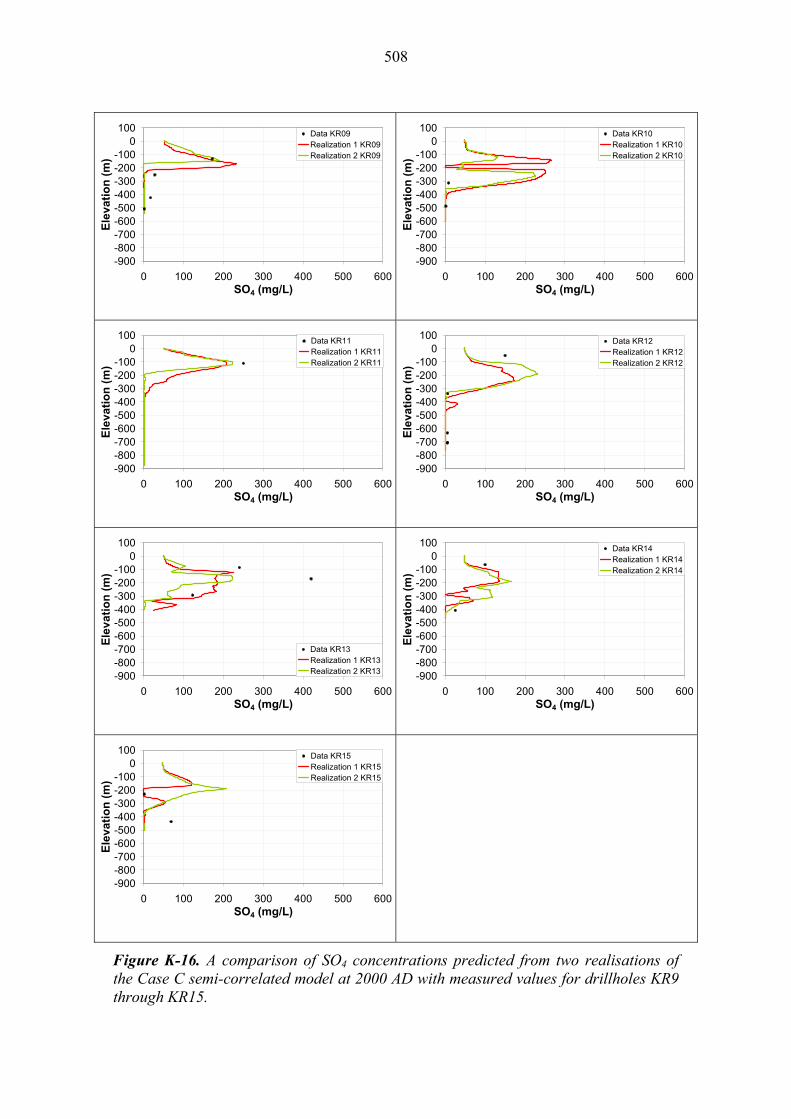
508
-900-800-700-600-500-400-300-200-100
0100
0 100 200 300 400 500 600SO4 (mg/L)
Ele
vati
on
(m
)
Data KR09Realization 1 KR09Realization 2 KR09
-900-800-700-600-500-400-300-200-100
0100
0 100 200 300 400 500 600SO4 (mg/L)
Ele
vati
on
(m
)
Data KR10Realization 1 KR10Realization 2 KR10
-900-800-700-600-500-400-300-200-100
0100
0 100 200 300 400 500 600SO4 (mg/L)
Ele
vati
on
(m
)
Data KR11Realization 1 KR11Realization 2 KR11
-900-800-700-600-500-400-300-200-100
0100
0 100 200 300 400 500 600SO4 (mg/L)
Ele
vati
on
(m
)
Data KR12Realization 1 KR12Realization 2 KR12
-900-800-700-600-500-400-300-200-100
0100
0 100 200 300 400 500 600SO4 (mg/L)
Ele
vati
on
(m
)
Data KR13Realization 1 KR13Realization 2 KR13 -900
-800-700-600-500-400-300-200-100
0100
0 100 200 300 400 500 600SO4 (mg/L)
Ele
vati
on
(m
)
Data KR14Realization 1 KR14Realization 2 KR14
-900-800-700-600-500-400-300-200-100
0100
0 100 200 300 400 500 600SO4 (mg/L)
Ele
vati
on
(m
)
Data KR15Realization 1 KR15Realization 2 KR15
Figure K-16. A comparison of SO4 concentrations predicted from two realisations of the Case C semi-correlated model at 2000 AD with measured values for drillholes KR9 through KR15.

509
K.3 Groundwater concentrations of bicarbonate
Comparisons of measured HCO3 concentrations in groundwater with predictions from two realisations of the Case A correlated and uncorrelated model, along with two realisations of the semi-correlated Case B and Case C models are detailed below. For each model case, results are presented on an individual drillhole basis for KR1 through KR15 in Figure K-17 to Figure K-24, although no measurements are available for comparison in drillholes KR13 and KR14. Greater variation in bicarbonate concentration with depth occurs between model realisations than for the corresponding groundwater head analysis in section K.1. From just two simulations, a number of measured HCO3 concentrations become realizable, and it is expected that if additional realisations were considered, a greater proportion of the concentrations observed would be captured within the envelope of results.

510
-900-800-700-600-500-400-300-200-100
0100
0 100 200 300 400 500 600HCO3 (mg/L)
Ele
vati
on
(m
)
Data KR01Realization 1 KR01Realization 2 KR01 -900
-800-700-600-500-400-300-200-100
0100
0 100 200 300 400 500 600HCO3 (mg/L)
Ele
vati
on
(m
)
Data KR02Realization 1 KR02Realization 2 KR02
-900-800-700-600-500-400-300-200-100
0100
0 100 200 300 400 500 600HCO3 (mg/L)
Ele
vati
on
(m
)
Data KR03Realization 1 KR03Realization 2 KR03
-900-800-700-600-500-400-300-200-100
0100
0 100 200 300 400 500 600HCO3 (mg/L)
Ele
vati
on
(m
)
Data KR04Realization 1 KR04Realization 2 KR04
-900-800-700-600-500-400-300-200-100
0100
0 100 200 300 400 500 600HCO3 (mg/L)
Ele
vati
on
(m
)
Data KR05Realization 1 KR05Realization 2 KR05 -900
-800-700-600-500-400-300-200-100
0100
0 100 200 300 400 500 600HCO3 (mg/L)
Ele
vati
on
(m
)
Data KR06Realization 1 KR06Realization 2 KR06
-900-800-700-600-500-400-300-200-100
0100
0 100 200 300 400 500 600HCO3 (mg/L)
Ele
vati
on
(m
)
Data KR07Realization 1 KR07Realization 2 KR07 -900
-800-700-600-500-400-300-200-100
0100
0 100 200 300 400 500 600HCO3 (mg/L)
Ele
vati
on
(m
)
Data KR08Realization 1 KR08Realization 2 KR08
Figure K-17. A comparison of HCO3 concentrations predicted from two realisations of the Case A correlated model at 2000 AD with measured values for drillholes KR1 through KR8.
511
-900-800-700-600-500-400-300-200-100
0100
0 100 200 300 400 500 600HCO3 (mg/L)
Ele
vati
on
(m
)
Data KR09Realization 1 KR09Realization 2 KR09 -900
-800-700-600-500-400-300-200-100
0100
0 100 200 300 400 500 600HCO3 (mg/L)
Ele
vati
on
(m
)
Data KR10Realization 1 KR10Realization 2 KR10
-900-800-700-600-500-400-300-200-100
0100
0 100 200 300 400 500 600HCO3 (mg/L)
Ele
vati
on
(m
)
Data KR11Realization 1 KR11Realization 2 KR11
-900-800-700-600-500-400-300-200-100
0100
0 100 200 300 400 500 600HCO3 (mg/L)
Ele
vati
on
(m
)
Data KR12Realization 1 KR12Realization 2 KR12
-900-800-700-600-500-400-300-200-100
0100
0 100 200 300 400 500 600HCO3 (mg/L)
Ele
vati
on
(m
)
Data KR13Realization 1 KR13Realization 2 KR13 -900
-800-700-600-500-400-300-200-100
0100
0 100 200 300 400 500 600HCO3 (mg/L)
Ele
vati
on
(m
)
Data KR14Realization 1 KR14Realization 2 KR14
-900-800-700-600-500-400-300-200-100
0100
0 100 200 300 400 500 600HCO3 (mg/L)
Ele
vati
on
(m
)
Data KR15Realization 1 KR15Realization 2 KR15
Figure K-18. A comparison of HCO3 concentrations predicted from two realisations of the Case A correlated model at 2000 AD with measured values for drillholes KR9 through KR15.

512
-900-800-700-600-500-400-300-200-100
0100
0 100 200 300 400 500 600HCO3 (mg/L)
Ele
vati
on
(m
)
Data KR01Realization 1 KR01Realization 2 KR01 -900
-800-700-600-500-400-300-200-100
0100
0 100 200 300 400 500 600HCO3 (mg/L)
Ele
vati
on
(m
)
Data KR02Realization 1 KR02Realization 2 KR02
-900-800-700-600-500-400-300-200-100
0100
0 100 200 300 400 500 600HCO3 (mg/L)
Ele
vati
on
(m
)
Data KR03Realization 1 KR03Realization 2 KR03
-900-800-700-600-500-400-300-200-100
0100
0 100 200 300 400 500 600HCO3 (mg/L)
Ele
vati
on
(m
)
Data KR04Realization 1 KR04Realization 2 KR04
-900-800-700-600-500-400-300-200-100
0100
0 100 200 300 400 500 600HCO3 (mg/L)
Ele
vati
on
(m
)
Data KR05Realization 1 KR05Realization 2 KR05 -900
-800-700-600-500-400-300-200-100
0100
0 100 200 300 400 500 600HCO3 (mg/L)
Ele
vati
on
(m
)
Data KR06Realization 1 KR06Realization 2 KR06
-900-800-700-600-500-400-300-200-100
0100
0 100 200 300 400 500 600HCO3 (mg/L)
Ele
vati
on
(m
)
Data KR07Realization 1 KR07Realization 2 KR07 -900
-800-700-600-500-400-300-200-100
0100
0 100 200 300 400 500 600HCO3 (mg/L)
Ele
vati
on
(m
)
Data KR08Realization 1 KR08Realization 2 KR08
Figure K-19. A comparison of HCO3 concentrations predicted from two realisations of the Case A uncorrelated model at 2000 AD with measured values for drillholes KR1 through KR8.
513
-900-800-700-600-500-400-300-200-100
0100
0 100 200 300 400 500 600HCO3 (mg/L)
Ele
vati
on
(m
)
Data KR09Realization 1 KR09Realization 2 KR09 -900
-800-700-600-500-400-300-200-100
0100
0 100 200 300 400 500 600HCO3 (mg/L)
Ele
vati
on
(m
)
Data KR10Realization 1 KR10Realization 2 KR10
-900-800-700-600-500-400-300-200-100
0100
0 100 200 300 400 500 600HCO3 (mg/L)
Ele
vati
on
(m
)
Data KR11Realization 1 KR11Realization 2 KR11
-900-800-700-600-500-400-300-200-100
0100
0 100 200 300 400 500 600HCO3 (mg/L)
Ele
vati
on
(m
)
Data KR12Realization 1 KR12Realization 2 KR12
-900-800-700-600-500-400-300-200-100
0100
0 100 200 300 400 500 600HCO3 (mg/L)
Ele
vati
on
(m
)
Data KR13Realization 1 KR13Realization 2 KR13 -900
-800-700-600-500-400-300-200-100
0100
0 100 200 300 400 500 600HCO3 (mg/L)
Ele
vati
on
(m
)
Data KR14Realization 1 KR14Realization 2 KR14
-900-800-700-600-500-400-300-200-100
0100
0 100 200 300 400 500 600HCO3 (mg/L)
Ele
vati
on
(m
)
Data KR15Realization 1 KR15Realization 2 KR15
Figure K-20. A comparison of the HCO3 concentrations predicted from two realisations of the Case A uncorrelated model at 2000 AD with measured values for drillholes KR9 through KR15.
514
-900-800-700-600-500-400-300-200-100
0100
0 100 200 300 400 500 600HCO3 (mg/L)
Ele
vati
on
(m
)
Data KR01Realization 1 KR01Realization 2 KR01 -900
-800-700-600-500-400-300-200-100
0100
0 100 200 300 400 500 600HCO3 (mg/L)
Ele
vati
on
(m
)
Data KR02Realization 1 KR02Realization 2 KR02
-900-800-700-600-500-400-300-200-100
0100
0 100 200 300 400 500 600HCO3 (mg/L)
Ele
vati
on
(m
)
Data KR03Realization 1 KR03Realization 2 KR03
-900-800-700-600-500-400-300-200-100
0100
0 100 200 300 400 500 600HCO3 (mg/L)
Ele
vati
on
(m
)
Data KR04Realization 1 KR04Realization 2 KR04
-900-800-700-600-500-400-300-200-100
0100
0 100 200 300 400 500 600HCO3 (mg/L)
Ele
vati
on
(m
)
Data KR05Realization 1 KR05Realization 2 KR05 -900
-800-700-600-500-400-300-200-100
0100
0 100 200 300 400 500 600HCO3 (mg/L)
Ele
vati
on
(m
)
Data KR06Realization 1 KR06Realization 2 KR06
-900-800-700-600-500-400-300-200-100
0100
0 100 200 300 400 500 600HCO3 (mg/L)
Ele
vati
on
(m
)
Data KR07Realization 1 KR07Realization 2 KR07 -900
-800-700-600-500-400-300-200-100
0100
0 100 200 300 400 500 600HCO3 (mg/L)
Ele
vati
on
(m
)
Data KR08Realization 1 KR08Realization 2 KR08
Figure K-21. A comparison of HCO3 concentrations predicted from two realisations of the Case B semi-correlated model at 2000 AD with measured values for drillholes KR1 through KR8.
515
-900-800-700-600-500-400-300-200-100
0100
0 100 200 300 400 500 600HCO3 (mg/L)
Ele
vati
on
(m
)
Data KR09Realization 1 KR09Realization 2 KR09 -900
-800-700-600-500-400-300-200-100
0100
0 100 200 300 400 500 600HCO3 (mg/L)
Ele
vati
on
(m
)
Data KR10Realization 1 KR10Realization 2 KR10
-900-800-700-600-500-400-300-200-100
0100
0 100 200 300 400 500 600HCO3 (mg/L)
Ele
vati
on
(m
)
Data KR11Realization 1 KR11Realization 2 KR11
-900-800-700-600-500-400-300-200-100
0100
0 100 200 300 400 500 600HCO3 (mg/L)
Ele
vati
on
(m
)
Data KR12Realization 1 KR12Realization 2 KR12
-900-800-700-600-500-400-300-200-100
0100
0 100 200 300 400 500 600HCO3 (mg/L)
Ele
vati
on
(m
)
Data KR13Realization 1 KR13Realization 2 KR13 -900
-800-700-600-500-400-300-200-100
0100
0 100 200 300 400 500 600HCO3 (mg/L)
Ele
vati
on
(m
)
Data KR14Realization 1 KR14Realization 2 KR14
-900-800-700-600-500-400-300-200-100
0100
0 100 200 300 400 500 600HCO3 (mg/L)
Ele
vati
on
(m
)
Data KR15Realization 1 KR15Realization 2 KR15
Figure K-22. A comparison of HCO3 concentrations predicted from two realisations of the Case B semi-correlated model at 2000 AD with measured values for drillholes KR9 through KR15.
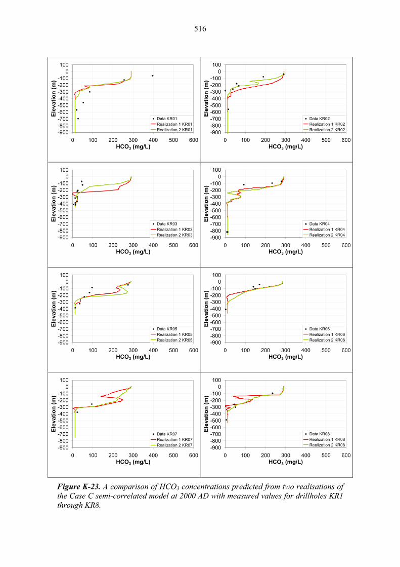
516
-900-800-700-600-500-400-300-200-100
0100
0 100 200 300 400 500 600HCO3 (mg/L)
Ele
vati
on
(m
)
Data KR01Realization 1 KR01Realization 2 KR01 -900
-800-700-600-500-400-300-200-100
0100
0 100 200 300 400 500 600HCO3 (mg/L)
Ele
vati
on
(m
)
Data KR02Realization 1 KR02Realization 2 KR02
-900-800-700-600-500-400-300-200-100
0100
0 100 200 300 400 500 600HCO3 (mg/L)
Ele
vati
on
(m
)
Data KR03Realization 1 KR03Realization 2 KR03
-900-800-700-600-500-400-300-200-100
0100
0 100 200 300 400 500 600HCO3 (mg/L)
Ele
vati
on
(m
)
Data KR04Realization 1 KR04Realization 2 KR04
-900-800-700-600-500-400-300-200-100
0100
0 100 200 300 400 500 600HCO3 (mg/L)
Ele
vati
on
(m
)
Data KR05Realization 1 KR05Realization 2 KR05 -900
-800-700-600-500-400-300-200-100
0100
0 100 200 300 400 500 600HCO3 (mg/L)
Ele
vati
on
(m
)
Data KR06Realization 1 KR06Realization 2 KR06
-900-800-700-600-500-400-300-200-100
0100
0 100 200 300 400 500 600HCO3 (mg/L)
Ele
vati
on
(m
)
Data KR07Realization 1 KR07Realization 2 KR07 -900
-800-700-600-500-400-300-200-100
0100
0 100 200 300 400 500 600HCO3 (mg/L)
Ele
vati
on
(m
)
Data KR08Realization 1 KR08Realization 2 KR08
Figure K-23. A comparison of HCO3 concentrations predicted from two realisations of the Case C semi-correlated model at 2000 AD with measured values for drillholes KR1 through KR8.
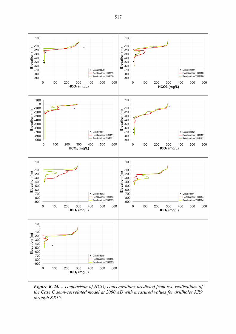
517
-900-800-700-600-500-400-300-200-100
0100
0 100 200 300 400 500 600HCO3 (mg/L)
Ele
vati
on
(m
)
Data KR09Realization 1 KR09Realization 2 KR09 -900
-800-700-600-500-400-300-200-100
0100
0 100 200 300 400 500 600HCO3 (mg/L)
Ele
vati
on
(m
)
Data KR10Realization 1 KR10Realization 2 KR10
-900-800-700-600-500-400-300-200-100
0100
0 100 200 300 400 500 600HCO3 (mg/L)
Ele
vati
on
(m
)
Data KR11Realization 1 KR11Realization 2 KR11
-900-800-700-600-500-400-300-200-100
0100
0 100 200 300 400 500 600HCO3 (mg/L)
Ele
vati
on
(m
)
Data KR12Realization 1 KR12Realization 2 KR12
-900-800-700-600-500-400-300-200-100
0100
0 100 200 300 400 500 600HCO3 (mg/L)
Ele
vati
on
(m
)
Data KR13Realization 1 KR13Realization 2 KR13 -900
-800-700-600-500-400-300-200-100
0100
0 100 200 300 400 500 600HCO3 (mg/L)
Ele
vati
on
(m
)
Data KR14Realization 1 KR14Realization 2 KR14
-900-800-700-600-500-400-300-200-100
0100
0 100 200 300 400 500 600HCO3 (mg/L)
Ele
vati
on
(m
)
Data KR15Realization 1 KR15Realization 2 KR15
Figure K-24. A comparison of HCO3 concentrations predicted from two realisations of the Case C semi-correlated model at 2000 AD with measured values for drillholes KR9 through KR15.

518
519
APPENDIX L: FRACTURE RETENTION CLASSES
Four fracture transport classes are defined in Section 4.8 for the filling minerals of fractures at Olkiluoto. These are
1. Fractures dominated by calcite;
2. Fractures dominated by hydrothermal clays;
3. Slickensided fractures;
4. Other fractures.
Specifically, fractures within the enhanced fracture database are assigned to one of four classes (TC1 through TC4) using the following logic:
a. Fractures are assigned to transport class Calcite if the fracture filling contains calcite or dolomite. The assumption is made that calcite- and dolomite- filled fractures are symptomatic of the same alteration state and are as equally likely to feature enhanced porosities.
b. Fractures are assigned to transport class Clay if the fracture filling contains ‘KA’, ‘KI’, ‘KS’, ‘IS’, ‘IL’, ‘MO’ or ‘SM’; if field KAOLINITE contains ‘KA’, field ILLITE contains ‘IL’, field MONTMORILLONITE contains ‘MO’, or field SMECTITE contains ‘SM’. Only clay minerals of hydrothermal origin are considered.
c. Fractures are assigned to transport class Slickenside if the fracture is in altered or weathered host rock, is in crush in unweathered rock, is a single individual fault or shear or shear zone. Fractures are also assigned to transport class Slickenside if the fracture is explicitly identified as a slickensided fracture or a fracture filled with soft material.
d. Any fracture not strictly meeting the aforementioned criteria is classified as transport class Other.
Application of the different fracture transport classes to the DFN model requires that the information on the different fracture types is conveyed from the geological analysis to the flow and transport analysis in the DFN model. As described in previous sections, fracture data is divided into four domains (NHU, CHUW, CHUE and SHU); four depth zones and three fracture orientation sets (N-S, E-W and SH). Since each fracture in the enhanced database is assigned a retention type, it would clearly be possible to calculate the percentages of fractures (either all fractures or PFL fractures) which are assigned to a particular retention type for each of the 48 different combinations of depth zone, domain and fracture orientation set. However, due to the uneven spread of fractures and PFL fractures across the 48 combinations, this approach is not robust statistically. To create a more robust solution, combinations exhibiting similar characteristics according to their depth zone, domain and fracture orientation set are aggregated together to form larger and therefore statistically more meaningful ensembles of data. The process by which this is achieved is described below.
Figure L-1 through to Figure L-6 show a series of plots which illustrate the percentage of fractures and PFL fractures by retention type, depth zone, domain and fracture set.
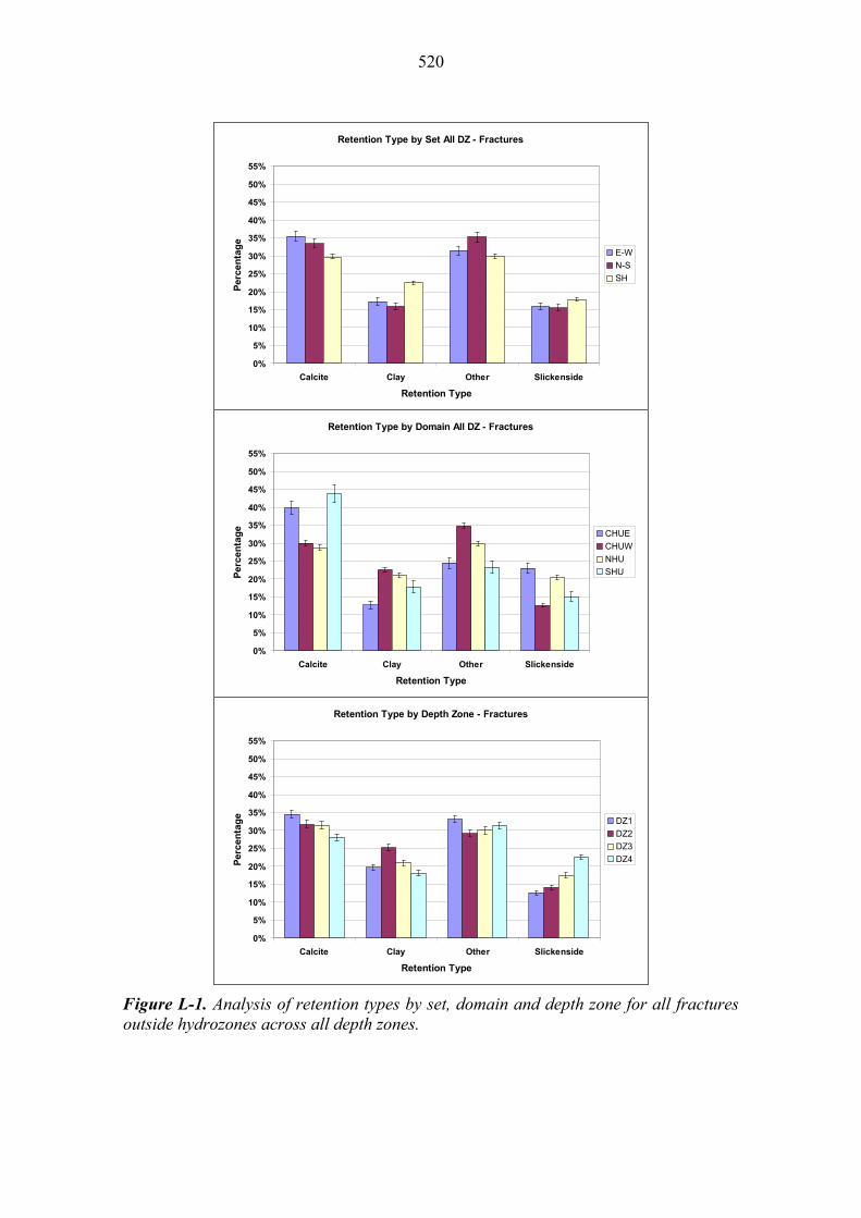
520
Retention Type by Set All DZ - Fractures
0%
5%
10%
15%
20%
25%
30%
35%
40%
45%
50%
55%
Calcite Clay Other Slickenside
Retention Type
Per
cen
tag
e
E-W
N-S
SH
Retention Type by Domain All DZ - Fractures
0%
5%
10%
15%
20%
25%
30%
35%
40%
45%
50%
55%
Calcite Clay Other Slickenside
Retention Type
Per
cen
tag
e
CHUE
CHUW
NHU
SHU
Retention Type by Depth Zone - Fractures
0%
5%
10%
15%
20%
25%
30%
35%
40%
45%
50%
55%
Calcite Clay Other Slickenside
Retention Type
Per
cen
tag
e
DZ1
DZ2
DZ3
DZ4
Figure L-1. Analysis of retention types by set, domain and depth zone for all fractures outside hydrozones across all depth zones.

521
Retention Type by Set All DZ - PFL
0%
5%
10%
15%
20%
25%
30%
35%
40%
45%
50%
55%
Calcite Clay Other Slickenside
Retention Type
Per
cen
tag
e
E-W
N-S
SH
Retention Type by Domain All DZ - PFL
0%
5%
10%
15%
20%
25%
30%
35%
40%
45%
50%
55%
Calcite Clay Other Slickenside
Retention Type
Per
cen
tag
e
CHUE
CHUW
NHU
SHU
Retention Type by Depth Zone - PFL
0%
5%
10%
15%
20%
25%
30%
35%
40%
45%
50%
55%
Calcite Clay Other Slickenside
Retention Type
Per
cen
tag
e
DZ1
DZ2
DZ3
DZ4
Figure L-2. Analysis of retention types by set, domain and depth zone for PFL fractures outside hydrozones across all depth zones.

522
Ret
enti
on
Typ
e b
y D
om
ain
DZ1
- F
ract
ure
s
0%5%
10%
15%
20%
25%
30%
35%
40%
45%
50%
55%
60%
Cal
cite
Cla
yO
the
rS
lick
en
sid
e
Ret
enti
on
Typ
e
Percentage
CH
UE
CH
UW
NH
U
SH
U
Ret
enti
on
Typ
e b
y D
om
ain
DZ2
- F
ract
ure
s
0%5%
10%
15%
20%
25%
30%
35%
40%
45%
50%
55%
60%
Cal
cite
Cla
yO
the
rS
lick
en
sid
e
Ret
enti
on
Typ
e
Percentage
CH
UE
CH
UW
NH
U
SH
U
Ret
enti
on
Typ
e b
y D
om
ain
DZ3
- F
ract
ure
s
0%5%
10%
15%
20%
25%
30%
35%
40%
45%
50%
55%
60%
Cal
cite
Cla
yO
the
rS
lick
en
sid
e
Ret
enti
on
Typ
e
Percentage
CH
UE
CH
UW
NH
U
SH
U
Ret
enti
on
Typ
e b
y D
om
ain
DZ4
- F
ract
ure
s
0%5%
10%
15%
20%
25%
30%
35%
40%
45%
50%
55%
60%
Cal
cite
Cla
yO
the
rS
lick
en
sid
e
Ret
enti
on
Typ
e
Percentage
CH
UE
CH
UW
NH
U
SH
U
Fig
ure
L-3
. A
naly
sis
of r
eten
tion
typ
es b
y do
mai
n in
eac
h de
pth
zone
for
all
fra
ctur
es o
utsi
de h
ydro
zone
s sh
owin
g pe
rcen
tage
of
all
frac
ture
s in
eac
h re
tent
ion
type
.
522
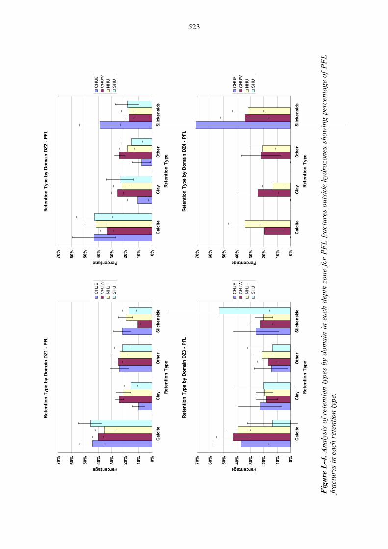
523
Ret
enti
on
Typ
e b
y D
om
ain
DZ1
- P
FL
0%
10%
20%
30%
40%
50%
60%
70%
Cal
cite
Cla
yO
the
rS
lick
en
sid
e
Ret
enti
on
Typ
e
Percentage
CH
UE
CH
UW
NH
U
SH
U
Ret
enti
on
Typ
e b
y D
om
ain
DZ2
- P
FL
0%
10%
20%
30%
40%
50%
60%
70%
Cal
cite
Cla
yO
the
rS
lick
en
sid
e
Ret
enti
on
Typ
e
Percentage
CH
UE
CH
UW
NH
U
SH
U
Ret
enti
on
Typ
e b
y D
om
ain
DZ3
- P
FL
0%
10%
20%
30%
40%
50%
60%
70%
Cal
cite
Cla
yO
the
rS
lick
en
sid
e
Ret
enti
on
Typ
e
Percentage
CH
UE
CH
UW
NH
U
SH
U
Ret
enti
on
Typ
e b
y D
om
ain
DZ4
- P
FL
0%
10%
20%
30%
40%
50%
60%
70%
Cal
cite
Cla
yO
the
rS
lick
en
sid
e
Ret
enti
on
Typ
e
Percentage
CH
UE
CH
UW
NH
U
SH
U
Fig
ure
L-4
. A
naly
sis
of r
eten
tion
typ
es b
y do
mai
n in
eac
h de
pth
zone
for
PF
L f
ract
ures
out
side
hyd
rozo
nes
show
ing
perc
enta
ge o
f P
FL
fr
actu
res
in e
ach
rete
ntio
n ty
pe.
523
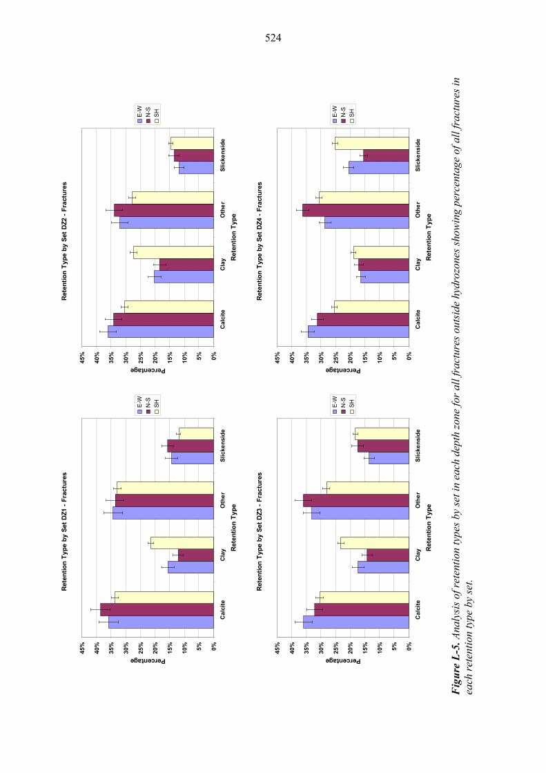
524
Ret
enti
on
Typ
e b
y S
et D
Z1 -
Fra
ctu
res
0%5%
10%
15%
20%
25%
30%
35%
40%
45%
Ca
lcit
eC
lay
Oth
er
Sli
cke
nsi
de
Ret
enti
on
Typ
e
Percentage
E-W
N-S
SH
Ret
enti
on
Typ
e b
y S
et D
Z2 -
Fra
ctu
res
0%5%
10%
15%
20%
25%
30%
35%
40%
45%
Ca
lcit
eC
lay
Oth
er
Sli
cke
nsi
de
Ret
enti
on
Typ
e
Percentage
E-W
N-S
SH
Ret
enti
on
Typ
e b
y S
et D
Z3 -
Fra
ctu
res
0%5%
10%
15%
20%
25%
30%
35%
40%
45%
Ca
lcit
eC
lay
Oth
er
Sli
cke
nsi
de
Ret
enti
on
Typ
e
Percentage
E-W
N-S
SH
Ret
enti
on
Typ
e b
y S
et D
Z4 -
Fra
ctu
res
0%5%
10%
15%
20%
25%
30%
35%
40%
45%
Ca
lcit
eC
lay
Oth
er
Sli
cke
nsi
de
Ret
enti
on
Typ
e
Percentage
E-W
N-S
SH
Fig
ure
L-5
. Ana
lysi
s of
ret
enti
on ty
pes
by s
et in
eac
h de
pth
zone
for
all f
ract
ures
out
side
hyd
rozo
nes
show
ing
perc
enta
ge o
f all
frac
ture
s in
ea
ch r
eten
tion
type
by
set.
524
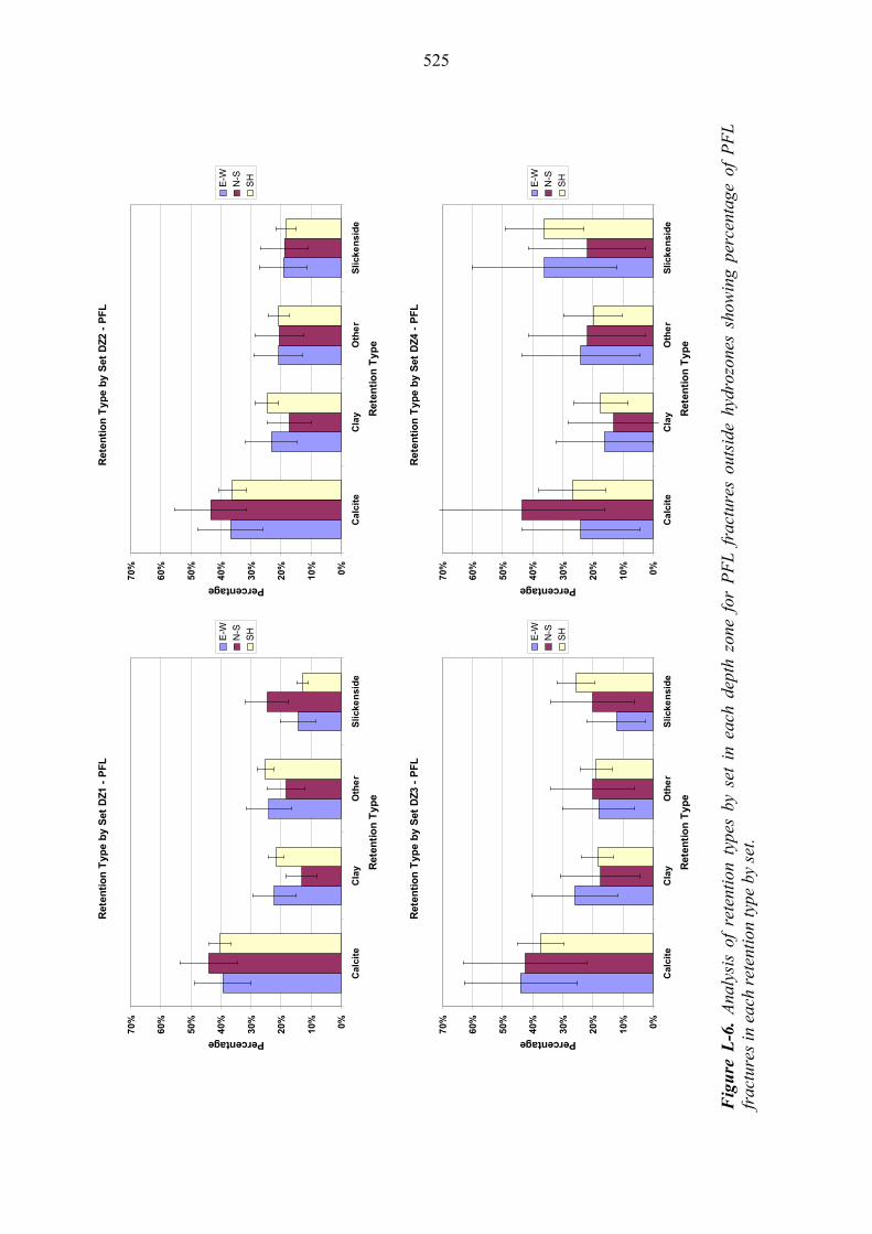
525
Ret
enti
on
Typ
e b
y S
et D
Z1 -
PF
L
0%
10%
20%
30%
40%
50%
60%
70%
Ca
lcit
eC
lay
Oth
er
Sli
cke
nsi
de
Ret
enti
on
Typ
e
Percentage
E-W
N-S
SH
Ret
enti
on
Typ
e b
y S
et D
Z2 -
PF
L
0%
10%
20%
30%
40%
50%
60%
70%
Ca
lcit
eC
lay
Oth
er
Sli
cke
nsi
de
Ret
enti
on
Typ
e
Percentage
E-W
N-S
SH
Ret
enti
on
Typ
e b
y S
et D
Z3 -
PF
L
0%
10%
20%
30%
40%
50%
60%
70%
Ca
lcit
eC
lay
Oth
er
Sli
cke
nsi
de
Ret
enti
on
Typ
e
Percentage
E-W
N-S
SH
Ret
enti
on
Typ
e b
y S
et D
Z4 -
PF
L
0%
10%
20%
30%
40%
50%
60%
70%
Ca
lcit
eC
lay
Oth
er
Sli
cke
nsi
de
Ret
enti
on
Typ
e
Percentage
E-W
N-S
SH
Fig
ure
L-6
. A
naly
sis
of r
eten
tion
typ
es b
y se
t in
eac
h de
pth
zone
for
PF
L f
ract
ures
out
side
hyd
rozo
nes
show
ing
perc
enta
ge o
f P
FL
fr
actu
res
in e
ach
rete
ntio
n ty
pe b
y se
t.
525
526
The following observations can be made by inspection of Figure L-1 through to Figure L-6:
By depth. Similar depth trends are observed for Calcite and Slickenside, in both fractures and PFL fractures. For calcite the percentage of calcite decreases with depth, while for slickenside there is a corresponding increase. Clay shows a significant depth trend from DZ2 to DZ4 in fractures but a smaller reduction in DZ4 for PFL fractures. Others remain fairly constant with depth for both all fractures and PFL fractures.
By fracture set. For PFL fractures, differences between E-W and SH set are small for all retention types, with slightly more variability observed with N-S although differences are not statistically significant apart from N-S lower for clay (which is also seen in all fractures). An increase in Slickenside with depth is clear for all orientations and SH set, but is not so clear for sub-vertical. A decrease for Calcite is clear for all orientations and SH set, not so clear for sub-vertical, especially N-S. There is a slight decrease in Clay in DZ3 and DZ4 fairly consistent across all sets.
By domain. Greater variability is observed between domains than between sets,
for both all fractures and PFL fractures although no discernable pattern is observed. A similar pattern between domains is observed for PFL fractures as for all fractures. For PFL fractures, CHUE is different for Clay and Slickenside; SHU can be assumed to be the same as NHU. CHUW has slight differences to NHU. Differences for CHUE in Clay are limited to DZ1 and DZ2 and only just statistically significant. Calcite increases and Other decreases.
It is clear from these figures and the observations above that there are no clear and unambiguous trends that can be drawn from figures and observations above. Any conclusions therefore contain an element of subjectivity. However, the following conclusions are made: Base the distribution between retention types on the count of PFL fractures in
each retention type rather than all fractures; Apply a depth trend for each retention type by dividing the total PFL count for
each retention class according to the PFL count for each retention type in each depth zone;
Combine N-S and E-W into a single group called Sub-vertical and then further subdivide the PFL count in each depth zone according to the number of PFL fractures in each Sub-horizontal (SH) and Sub-vertical orientation set;
And finally, further subdivide the PFL count in each Sub-vertical and Sub-horizontal orientation set in each depth zone according to whether the PFL lies in the CHUE or non-CHUE hydraulic domain.
Figure 4-32 and Table 4-11 detail retention type percentages based on the above conclusions.
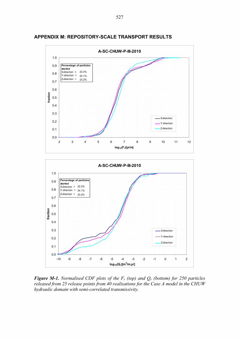
527
APPENDIX M: REPOSITORY-SCALE TRANSPORT RESULTS
A-SC-CHUW-P-III-2010
0.0
0.1
0.2
0.3
0.4
0.5
0.6
0.7
0.8
0.9
1.0
2 3 4 5 6 7 8 9 10 11 12
log10(Fr)[yr/m]
frac
tio
n
X-direction
Y-direction
Z-direction
Percentage of particles started X-direction = Y-direction =
Z-direction = 24.1%
22.2%
23.2%
A-SC-CHUW-P-III-2010
0.0
0.1
0.2
0.3
0.4
0.5
0.6
0.7
0.8
0.9
1.0
-10 -9 -8 -7 -6 -5 -4 -3 -2 -1 0 1 2
log10(Qr)[m3/m,yr]
frac
tio
n
X-direction
Y-direction
Z-direction
Percentage of particles started X-direction = Y-direction =
Z-direction =
22.2%
24.1%
23.2%
Figure M-1. Normalised CDF plots of the Fr (top) and Qr (bottom) for 250 particles released from 25 release points from 40 realisations for the Case A model in the CHUW hydraulic domain with semi-correlated transmissivity.
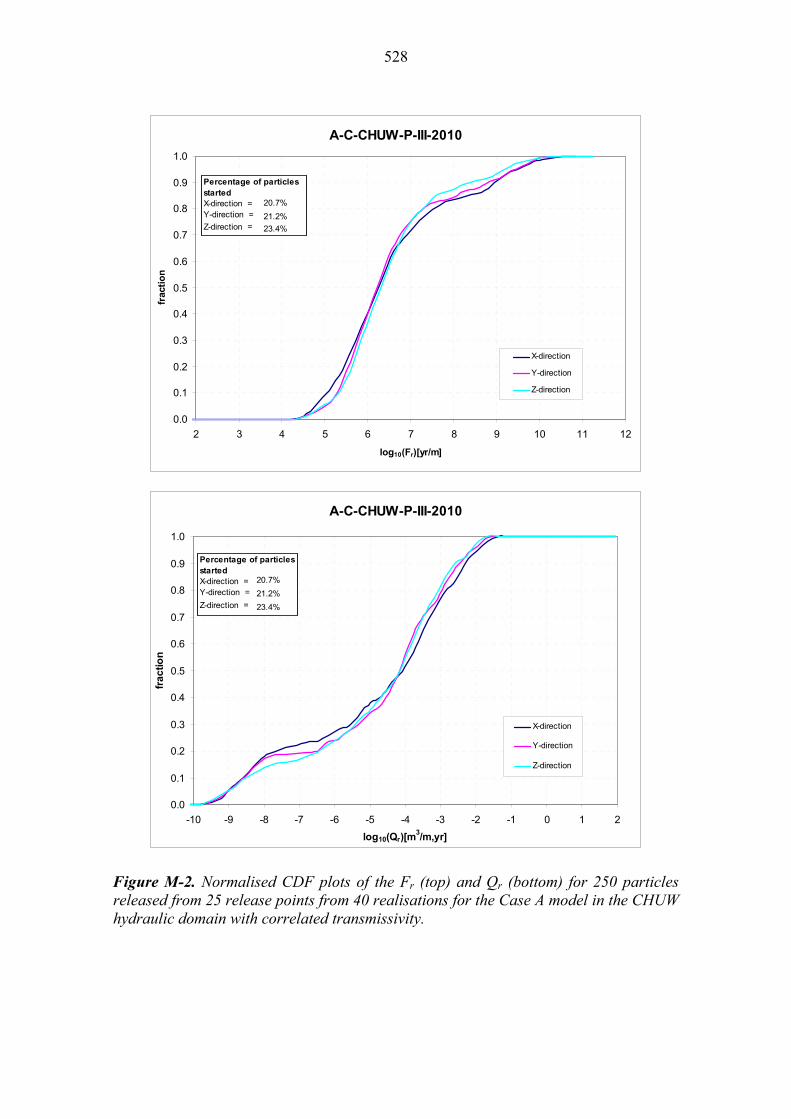
528
A-C-CHUW-P-III-2010
0.0
0.1
0.2
0.3
0.4
0.5
0.6
0.7
0.8
0.9
1.0
2 3 4 5 6 7 8 9 10 11 12
log10(Fr)[yr/m]
frac
tio
n
X-direction
Y-direction
Z-direction
Percentage of particles started X-direction = Y-direction =
Z-direction = 21.2%
20.7%
23.4%
A-C-CHUW-P-III-2010
0.0
0.1
0.2
0.3
0.4
0.5
0.6
0.7
0.8
0.9
1.0
-10 -9 -8 -7 -6 -5 -4 -3 -2 -1 0 1 2
log10(Qr)[m3/m,yr]
frac
tio
n
X-direction
Y-direction
Z-direction
Percentage of particles started X-direction = Y-direction =
Z-direction =
20.7%
21.2%
23.4%
Figure M-2. Normalised CDF plots of the Fr (top) and Qr (bottom) for 250 particles released from 25 release points from 40 realisations for the Case A model in the CHUW hydraulic domain with correlated transmissivity.
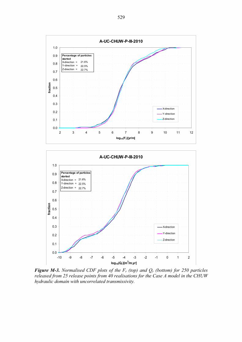
529
A-UC-CHUW-P-III-2010
0.0
0.1
0.2
0.3
0.4
0.5
0.6
0.7
0.8
0.9
1.0
2 3 4 5 6 7 8 9 10 11 12
log10(Fr)[yr/m]
frac
tio
n
X-direction
Y-direction
Z-direction
Percentage of particles started X-direction = Y-direction =
Z-direction = 22.5%
21.6%
22.7%
A-UC-CHUW-P-III-2010
0.0
0.1
0.2
0.3
0.4
0.5
0.6
0.7
0.8
0.9
1.0
-10 -9 -8 -7 -6 -5 -4 -3 -2 -1 0 1 2
log10(Qr)[m3/m,yr]
frac
tio
n
X-direction
Y-direction
Z-direction
Percentage of particles started X-direction = Y-direction =
Z-direction =
21.6%
22.5%
22.7%
Figure M-3. Normalised CDF plots of the Fr (top) and Qr (bottom) for 250 particles released from 25 release points from 40 realisations for the Case A model in the CHUW hydraulic domain with uncorrelated transmissivity.
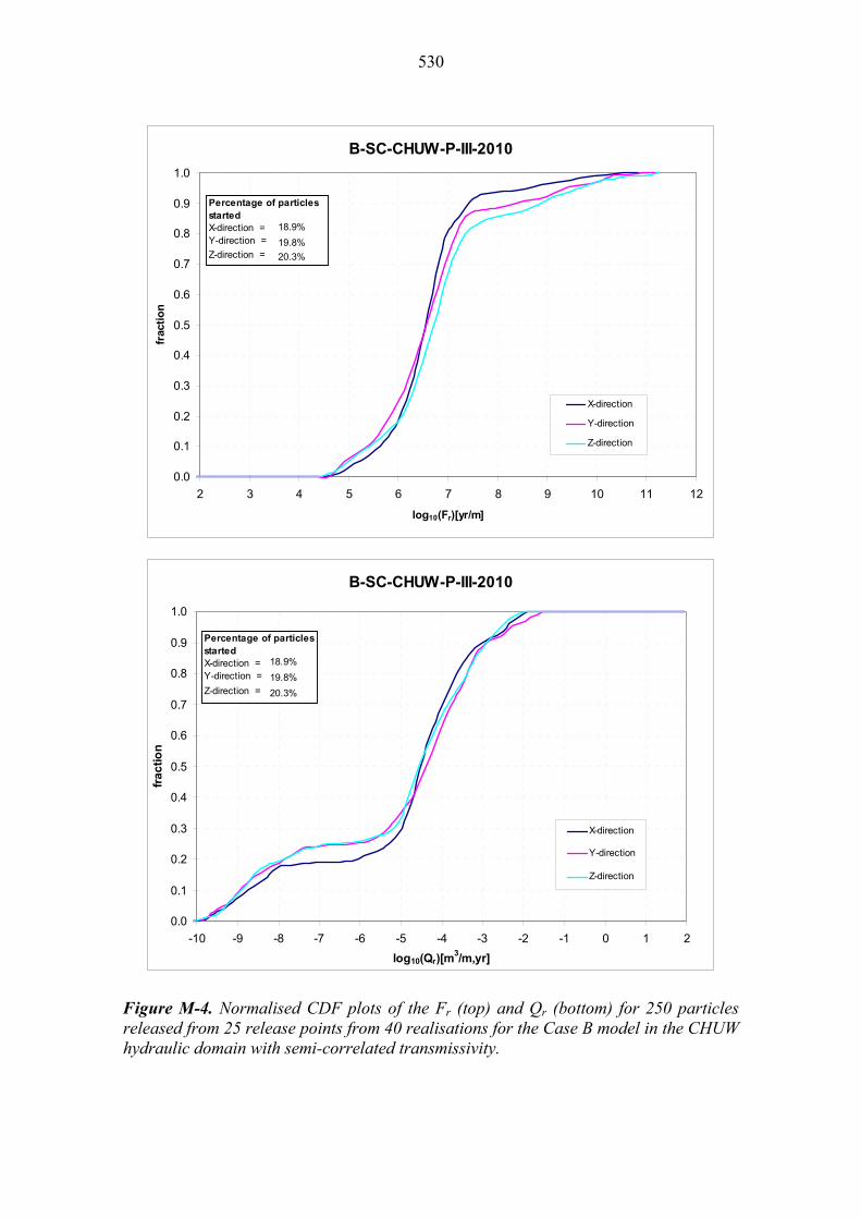
530
B-SC-CHUW-P-III-2010
0.0
0.1
0.2
0.3
0.4
0.5
0.6
0.7
0.8
0.9
1.0
2 3 4 5 6 7 8 9 10 11 12
log10(Fr)[yr/m]
frac
tio
n
X-direction
Y-direction
Z-direction
Percentage of particles started X-direction = Y-direction =
Z-direction = 19.8%
18.9%
20.3%
B-SC-CHUW-P-III-2010
0.0
0.1
0.2
0.3
0.4
0.5
0.6
0.7
0.8
0.9
1.0
-10 -9 -8 -7 -6 -5 -4 -3 -2 -1 0 1 2
log10(Qr)[m3/m,yr]
fra
cti
on
X-direction
Y-direction
Z-direction
Percentage of particles started X-direction = Y-direction =
Z-direction =
18.9%
19.8%
20.3%
Figure M-4. Normalised CDF plots of the Fr (top) and Qr (bottom) for 250 particles released from 25 release points from 40 realisations for the Case B model in the CHUW hydraulic domain with semi-correlated transmissivity.

531
C-SC-CHUW-P-III-2010
0.0
0.1
0.2
0.3
0.4
0.5
0.6
0.7
0.8
0.9
1.0
2 3 4 5 6 7 8 9 10 11 12
log10(Fr)[yr/m]
frac
tio
n
X-direction
Y-direction
Z-direction
Percentage of particles started X-direction = Y-direction =
Z-direction = 25.2%
22.9%
27.6%
C-SC-CHUW-P-III-2010
0.0
0.1
0.2
0.3
0.4
0.5
0.6
0.7
0.8
0.9
1.0
-10 -9 -8 -7 -6 -5 -4 -3 -2 -1 0 1 2
log10(Qr)[m3/m,yr]
fra
cti
on
X-direction
Y-direction
Z-direction
Percentage of particles started X-direction = Y-direction =
Z-direction =
22.9%
25.2%
27.6%
Figure M-5. Normalised CDF plots of the Fr (top) and Qr (bottom) for 250 particles released from 25 release points from 40 realisations for the Case C model in the CHUW hydraulic domain with semi-correlated transmissivity.
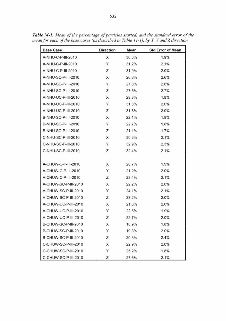
532
Table M-1. Mean of the percentage of particles started, and the standard error of the mean for each of the base cases (as described in Table 11-1), by X, Y and Z direction.
Base Case Direction Mean Std Error of Mean
A-NHU-C-P-III-2010 X 30.3% 1.9%
A-NHU-C-P-III-2010 Y 31.2% 2.1%
A-NHU-C-P-III-2010 Z 31.9% 2.0%
A-NHU-SC-P-III-2010 X 26.8% 2.6%
A-NHU-SC-P-III-2010 Y 27.8% 2.6%
A-NHU-SC-P-III-2010 Z 27.5% 2.7%
A-NHU-UC-P-III-2010 X 29.3% 1.8%
A-NHU-UC-P-III-2010 Y 31.8% 2.0%
A-NHU-UC-P-III-2010 Z 31.8% 2.0%
B-NHU-SC-P-III-2010 X 22.1% 1.8%
B-NHU-SC-P-III-2010 Y 22.7% 1.8%
B-NHU-SC-P-III-2010 Z 21.1% 1.7%
C-NHU-SC-P-III-2010 X 30.3% 2.1%
C-NHU-SC-P-III-2010 Y 32.9% 2.3%
C-NHU-SC-P-III-2010 Z 32.4% 2.1%
A-CHUW-C-P-III-2010 X 20.7% 1.9%
A-CHUW-C-P-III-2010 Y 21.2% 2.0%
A-CHUW-C-P-III-2010 Z 23.4% 2.1%
A-CHUW-SC-P-III-2010 X 22.2% 2.0%
A-CHUW-SC-P-III-2010 Y 24.1% 2.1%
A-CHUW-SC-P-III-2010 Z 23.2% 2.0%
A-CHUW-UC-P-III-2010 X 21.6% 2.0%
A-CHUW-UC-P-III-2010 Y 22.5% 1.9%
A-CHUW-UC-P-III-2010 Z 22.7% 2.0%
B-CHUW-SC-P-III-2010 X 18.9% 1.8%
B-CHUW-SC-P-III-2010 Y 19.8% 2.0%
B-CHUW-SC-P-III-2010 Z 20.3% 2.4%
C-CHUW-SC-P-III-2010 X 22.9% 2.0%
C-CHUW-SC-P-III-2010 Y 25.2% 1.8%
C-CHUW-SC-P-III-2010 Z 27.6% 2.1%
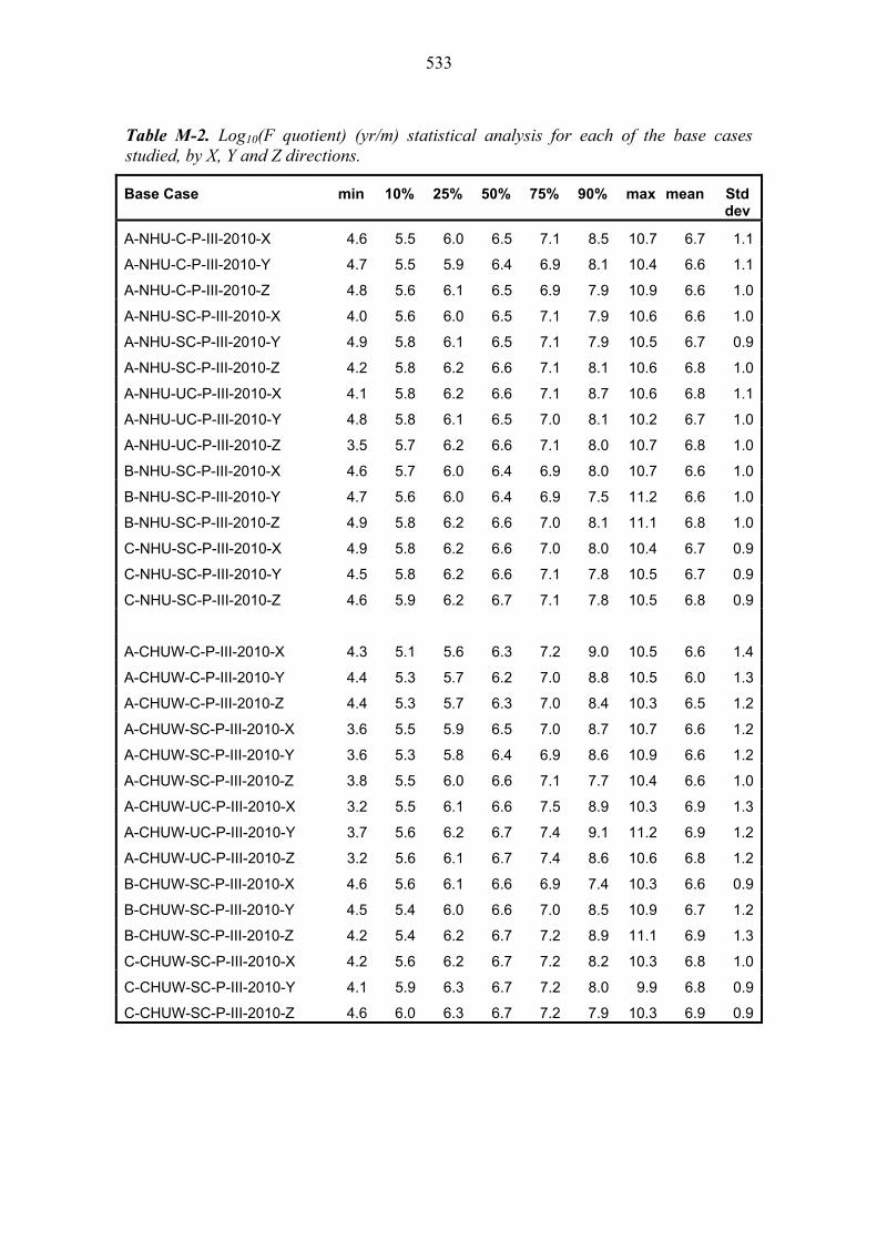
533
Table M-2. Log10(F quotient) (yr/m) statistical analysis for each of the base cases studied, by X, Y and Z directions.
Base Case min 10% 25% 50% 75% 90% max mean Std dev
A-NHU-C-P-III-2010-X 4.6 5.5 6.0 6.5 7.1 8.5 10.7 6.7 1.1
A-NHU-C-P-III-2010-Y 4.7 5.5 5.9 6.4 6.9 8.1 10.4 6.6 1.1
A-NHU-C-P-III-2010-Z 4.8 5.6 6.1 6.5 6.9 7.9 10.9 6.6 1.0
A-NHU-SC-P-III-2010-X 4.0 5.6 6.0 6.5 7.1 7.9 10.6 6.6 1.0
A-NHU-SC-P-III-2010-Y 4.9 5.8 6.1 6.5 7.1 7.9 10.5 6.7 0.9
A-NHU-SC-P-III-2010-Z 4.2 5.8 6.2 6.6 7.1 8.1 10.6 6.8 1.0
A-NHU-UC-P-III-2010-X 4.1 5.8 6.2 6.6 7.1 8.7 10.6 6.8 1.1
A-NHU-UC-P-III-2010-Y 4.8 5.8 6.1 6.5 7.0 8.1 10.2 6.7 1.0
A-NHU-UC-P-III-2010-Z 3.5 5.7 6.2 6.6 7.1 8.0 10.7 6.8 1.0
B-NHU-SC-P-III-2010-X 4.6 5.7 6.0 6.4 6.9 8.0 10.7 6.6 1.0
B-NHU-SC-P-III-2010-Y 4.7 5.6 6.0 6.4 6.9 7.5 11.2 6.6 1.0
B-NHU-SC-P-III-2010-Z 4.9 5.8 6.2 6.6 7.0 8.1 11.1 6.8 1.0
C-NHU-SC-P-III-2010-X 4.9 5.8 6.2 6.6 7.0 8.0 10.4 6.7 0.9
C-NHU-SC-P-III-2010-Y 4.5 5.8 6.2 6.6 7.1 7.8 10.5 6.7 0.9
C-NHU-SC-P-III-2010-Z 4.6 5.9 6.2 6.7 7.1 7.8 10.5 6.8 0.9
A-CHUW-C-P-III-2010-X 4.3 5.1 5.6 6.3 7.2 9.0 10.5 6.6 1.4
A-CHUW-C-P-III-2010-Y 4.4 5.3 5.7 6.2 7.0 8.8 10.5 6.0 1.3
A-CHUW-C-P-III-2010-Z 4.4 5.3 5.7 6.3 7.0 8.4 10.3 6.5 1.2
A-CHUW-SC-P-III-2010-X 3.6 5.5 5.9 6.5 7.0 8.7 10.7 6.6 1.2
A-CHUW-SC-P-III-2010-Y 3.6 5.3 5.8 6.4 6.9 8.6 10.9 6.6 1.2
A-CHUW-SC-P-III-2010-Z 3.8 5.5 6.0 6.6 7.1 7.7 10.4 6.6 1.0
A-CHUW-UC-P-III-2010-X 3.2 5.5 6.1 6.6 7.5 8.9 10.3 6.9 1.3
A-CHUW-UC-P-III-2010-Y 3.7 5.6 6.2 6.7 7.4 9.1 11.2 6.9 1.2
A-CHUW-UC-P-III-2010-Z 3.2 5.6 6.1 6.7 7.4 8.6 10.6 6.8 1.2
B-CHUW-SC-P-III-2010-X 4.6 5.6 6.1 6.6 6.9 7.4 10.3 6.6 0.9
B-CHUW-SC-P-III-2010-Y 4.5 5.4 6.0 6.6 7.0 8.5 10.9 6.7 1.2
B-CHUW-SC-P-III-2010-Z 4.2 5.4 6.2 6.7 7.2 8.9 11.1 6.9 1.3
C-CHUW-SC-P-III-2010-X 4.2 5.6 6.2 6.7 7.2 8.2 10.3 6.8 1.0
C-CHUW-SC-P-III-2010-Y 4.1 5.9 6.3 6.7 7.2 8.0 9.9 6.8 0.9
C-CHUW-SC-P-III-2010-Z 4.6 6.0 6.3 6.7 7.2 7.9 10.3 6.9 0.9

534
Table M-3. Log10(Flow-rate per unit width (Q)) (m3/m, yr) statistical analysis for each of the base cases studied by X, Y and Z directions.
Base Case min 10% 25% 50% 75% 90% max mean Std dev
A-NHU-C-P-III-2010-X -10.1 -8.4 -5.8 -4.1 -3.4 -2.6 -1.6 -4.8 2.1
A-NHU-C-P-III-2010-Y -10.0 -8.3 -5.2 -4.0 -3.3 -2.6 -1.8 -4.6 2.0
A-NHU-C-P-III-2010-Z -10.2 -8.2 -5.0 -4.2 -3.4 -2.7 -1.8 -4.6 1.9
A-NHU-SC-P-III-2010-X -10.6 -7.9 -5.3 -4.2 -3.4 -2.9 -1.6 -4.7 1.8
A-NHU-SC-P-III-2010-Y -9.9 -8.2 -5.2 -4.1 -3.4 -2.9 -1.8 -4.7 1.9
A-NHU-SC-P-III-2010-Z -10.0 -8.0 -5.4 -4.2 -3.5 -3.0 -1.5 -4.8 1.8
A-NHU-UC-P-III-2010-X -10.3 -8.7 -6.9 -4.3 -3.5 -3.0 -1.4 -5.1 2.2
A-NHU-UC-P-III-2010-Y -10.3 -8.3 -5.5 -4.1 -3.4 -2.9 -2.0 -4.8 2.0
A-NHU-UC-P-III-2010-Z -10.7 -8.4 -5.3 -4.2 -3.5 -2.9 -1.3 -4.8 1.9
B-NHU-SC-P-III-2010-X -10.6 -8.7 -5.5 -4.1 -3.3 -2.8 -2.0 -4.9 2.2
B-NHU-SC-P-III-2010-Y -10.6 -8.8 -5.7 -4.1 -3.5 -2.9 -1.8 -4.9 2.1
B-NHU-SC-P-III-2010-Z -10.5 -8.9 -5.5 -4.3 -3.6 -3.1 -2.0 -5.1 2.1
C-NHU-SC-P-III-2010-X -10.6 -8.0 -5.3 -4.2 -3.5 -2.8 -1.5 -4.7 1.8
C-NHU-SC-P-III-2010-Y -9.9 -7.5 -5.2 -4.3 -3.6 -2.9 -1.7 -4.7 1.7
C-NHU-SC-P-III-2010-Z -10.1 -7.2 -5.2 -4.2 -3.4 -3.0 -2.0 -4.6 1.7
A-CHUW-C-P-III-2010-X -9.9 -8.6 -6.4 -4.0 -3.1 -2.4 -1.4 -4.8 2.3
A-CHUW-C-P-III-2010-Y -9.8 -8.5 -5.8 -4.2 -3.2 -2.5 -1.4 -4.8 2.2
A-CHUW-C-P-III-2010-Z -10.5 -8.5 -5.8 -4.2 -3.3 -2.6 -1.8 -4.8 2.1
A-CHUW-SC-P-III-2010-X -10.7 -8.5 -6.2 -4.2 -3.5 -2.8 -0.9 -5.0 2.1
A-CHUW-SC-P-III-2010-Y -10.0 -8.5 -5.5 -4.1 -3.3 -2.8 -0.5 -4.8 2.1
A-CHUW-SC-P-III-2010-Z -10.0 -7.2 -5.2 -4.3 -3.5 -2.7 -1.0 -4.6 1.8
A-CHUW-UC-P-III-2010-X -9.9 -8.4 -6.0 -4.3 -3.5 -2.9 -0.3 -5.0 2.0
A-CHUW-UC-P-III-2010-Y -10.6 -8.7 -6.4 -4.6 -3.7 -3.1 -0.7 -5.2 2.1
A-CHUW-UC-P-III-2010-Z -9.9 -8.6 -6.3 -4.5 -3.7 -2.9 -0.7 -5.1 2.0
B-CHUW-SC-P-III-2010-X -10.0 -8.8 -5.3 -4.5 -3.8 -3.0 -2.0 -5.0 2.0
B-CHUW-SC-P-III-2010-Y -10.1 -9.0 -6.2 -4.4 -3.6 -2.9 -1.6 -5.1 2.2
B-CHUW-SC-P-III-2010-Z -10.3 -8.9 -6.9 -4.6 -3.6 -2.9 -2.1 -5.2 2.2
C-CHUW-SC-P-III-2010-X -9.9 -8.0 -5.6 -4.5 -3.7 -3.2 -1.4 -5.0 1.8
C-CHUW-SC-P-III-2010-Y -10.5 -7.6 -5.2 -4.4 -3.8 -3.4 -2.0 -4.8 1.6
C-CHUW-SC-P-III-2010-Z -10.0 -7.0 -5.4 -4.4 -3.9 -3.4 -1.6 -4.8 1.5

535
Table M-4. Log10(travel times) (yr) statistical analysis for each base case studied in X, Y and Z directions.
Base Case min 10% 25% 50% 75% 90% max mean Std dev
A-NHU-C-P-III-2010-X 0.5 1.3 1.7 2.1 2.6 3.9 6.3 2.3 1.0
A-NHU-C-P-III-2010-Y 0.7 1.3 1.6 2.0 2.5 3.5 5.9 2.2 0.9
A-NHU-C-P-III-2010-Z 0.8 1.4 1.7 2.1 2.5 3.3 6.4 2.3 0.9
A-NHU-SC-P-III-2010-X 0.1 1.4 1.7 2.1 2.6 3.3 6.1 2.3 0.9
A-NHU-SC-P-III-2010-Y 0.9 1.5 1.8 2.1 2.6 3.4 6.0 2.3 0.8
A-NHU-SC-P-III-2010-Z 0.4 1.6 1.9 2.2 2.7 3.6 6.2 2.4 0.9
A-NHU-UC-P-III-2010-X 0.2 1.6 1.9 2.3 2.9 4.5 2.1 2.6 1.1
A-NHU-UC-P-III-2010-Y 0.6 1.6 1.9 2.2 2.7 3.8 6.0 2.5 1.0
A-NHU-UC-P-III-2010-Z -0.1 1.6 2.0 2.4 2.8 3.8 6.1 2.5 1.0
B-NHU-SC-P-III-2010-X 0.8 1.5 1.8 2.2 2.6 3.7 6.3 2.4 1.0
B-NHU-SC-P-III-2010-Y 0.9 1.5 1.8 2.2 2.6 3.3 7.1 2.4 1.0
B-NHU-SC-P-III-2010-Z 0.9 1.7 2.0 2.3 2.7 3.7 7.0 2.6 1.0
C-NHU-SC-P-III-2010-X 0.9 1.7 2.0 2.3 2.7 3.5 6.1 2.5 0.8
C-NHU-SC-P-III-2010-Y 0.7 1.7 2.0 2.4 2.8 3.4 6.0 2.5 0.8
C-NHU-SC-P-III-2010-Z 0.7 1.8 2.1 2.5 2.9 3.4 6.4 2.6 0.8
A-CHUW-C-P-III-2010-X 0.4 0.9 1.3 1.9 2.8 3.3 6.0 2.3 1.3
A-CHUW-C-P-III-2010-Y 0.5 1.1 1.4 1.9 2.6 4.2 6.0 2.2 1.2
A-CHUW-C-P-III-2010-Z 0.4 1.2 1.5 2.0 2.6 3.8 5.8 2.2 1.1
A-CHUW-SC-P-III-2010-X 0.0 1.3 1.6 2.1 2.6 4.0 6.4 2.3 1.1
A-CHUW-SC-P-III-2010-Y 0.0 1.1 1.6 2.0 2.5 4.1 6.4 2.2 1.1
A-CHUW-SC-P-III-2010-Z 0.2 1.3 1.8 2.0 2.7 3.4 5.8 2.3 0.9
A-CHUW-UC-P-III-2010-X -0.3 1.3 1.9 2.4 3.2 4.6 6.0 2.6 1.2
A-CHUW-UC-P-III-2010-Y 0.2 1.5 1.9 2.4 3.1 4.5 7.0 2.7 1.2
A-CHUW-UC-P-III-2010-Z -0.4 1.4 1.9 2.4 3.1 4.3 6.2 2.6 1.1
B-CHUW-SC-P-III-2010-X 0.7 1.5 1.9 2.3 2.6 3.1 5.9 2.3 0.8
B-CHUW-SC-P-III-2010-Y 0.6 1.3 1.8 2.3 2.7 3.9 6.7 2.4 1.1
B-CHUW-SC-P-III-2010-Z 0.4 1.3 2.0 2.4 2.9 4.5 6.9 2.6 1.2
C-CHUW-SC-P-III-2010-X 0.5 1.5 2.0 2.5 3.0 3.7 6.0 2.6 0.9
C-CHUW-SC-P-III-2010-Y 0.4 1.8 2.1 2.5 2.9 3.7 5.7 2.6 0.8
C-CHUW-SC-P-III-2010-Z 0.8 1.9 2.2 2.5 3.0 3.6 6.1 2.7 0.8
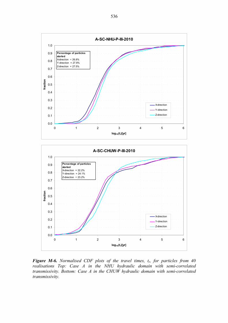
536
A-SC-NHU-P-III-2010
0.0
0.1
0.2
0.3
0.4
0.5
0.6
0.7
0.8
0.9
1.0
0 1 2 3 4 5 6
log10(tr)[yr]
frac
tio
n
X-direction
Y-direction
Z-direction
Percentage of particles started X-direction = 26.8%Y-direction = 27.8%
Z-direction = 27.5%
A-SC-CHUW-P-III-2010
0.0
0.1
0.2
0.3
0.4
0.5
0.6
0.7
0.8
0.9
1.0
0 1 2 3 4 5 6
log10(tr)[yr]
frac
tio
n
X-direction
Y-direction
Z-direction
Percentage of particles started X-direction = 22.2%Y-direction = 24.1%
Z-direction = 23.2%
Figure M-6. Normalised CDF plots of the travel times, tr, for particles from 40 realisations Top: Case A in the NHU hydraulic domain with semi-correlated transmissivity. Bottom: Case A in the CHUW hydraulic domain with semi-correlated transmissivity.

537
Log10(Fr) median, 10% and 90% percentiles
5
6
7
8
9
10
11
AC AS AU BS CS
Model Case
log
10(F
r [y/
m]) CHUW-X
NHU-X
CHUW-Y
NHU-YCHUW-Z
NHU-Z
log10(Fr) mean +- standard deviation
5
6
7
8
9
10
11
AC AS AU BS CS
Model Case
log
10(F
r [y
/m]) CHUW-X
NHU-XCHUW-Y
NHU-Y
CHUW-ZNHU-Z
Figure M-7. Minimum and median Fr of the simulated flow paths for different alternative DFN models and flow directions for the NHU domain in Depth Zone 4. Notations of the alternate models are Case A correlated transmissivity (AC); Case A semi-correlated transmissivity (AS); Case A uncorrelated transmissivity (AU); CaseB semi-correlated transmissivity (BS) and Case C semi-correlated transmissivity (CS). In the top graph vertical lines show 10 % to 90 % variability between different realisations. Median F of all realisations is shown by horizontal lines. In the bottom graph vertical lines show standard deviation variability between different realisations. Mean F of all realisations is shown by horizontal lines.
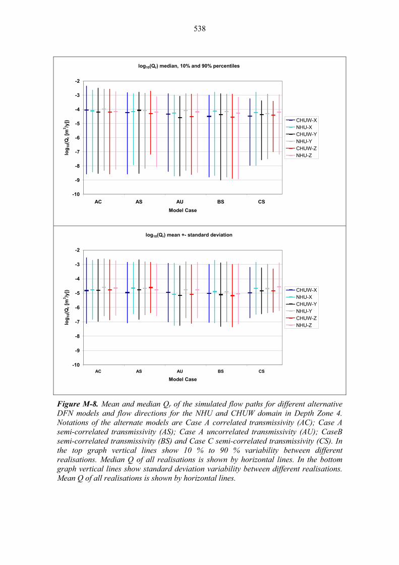
538
log10(Qr) median, 10% and 90% percentiles
-10
-9
-8
-7
-6
-5
-4
-3
-2
AC AS AU BS CS
Model Case
log
10(Q
r [m
3 /y]) CHUW-X
NHU-XCHUW-Y
NHU-Y
CHUW-ZNHU-Z
log10(Qr) mean +- standard deviation
-10
-9
-8
-7
-6
-5
-4
-3
-2
AC AS AU BS CS
Model Case
log
10(Q
r [m
3 /y]) CHUW-X
NHU-X
CHUW-YNHU-Y
CHUW-Z
NHU-Z
Figure M-8. Mean and median Qr of the simulated flow paths for different alternative DFN models and flow directions for the NHU and CHUW domain in Depth Zone 4. Notations of the alternate models are Case A correlated transmissivity (AC); Case A semi-correlated transmissivity (AS); Case A uncorrelated transmissivity (AU); CaseB semi-correlated transmissivity (BS) and Case C semi-correlated transmissivity (CS). In the top graph vertical lines show 10 % to 90 % variability between different realisations. Median Q of all realisations is shown by horizontal lines. In the bottom graph vertical lines show standard deviation variability between different realisations. Mean Q of all realisations is shown by horizontal lines.

539
log10(tr) mean, 10% and 90% perecentiles
0
1
2
3
4
5
6
7
AC AS AU BS CS
Model Case
log
10(t
r([y
])
CHUW-X
NHU-XCHUW-Y
NHU-Y
CHUW-ZNHU-Z
log10(tr) mean +- standard deviation
0
1
2
3
4
5
6
7
AC AS AU BS CS
Model Case
log
10(t
r[y]
)
CHUW-X
NHU-XCHUW-Y
NHU-Y
CHUW-ZNHU-Z
Figure M-9. Mean and median tr of the simulated flow paths for different alternative DFN models and flow directions for the NHU and CHUW domain in Depth Zone 4. Notations of the alternate models are Case A correlated transmissivity (AC); Case A semi-correlated transmissivity (AS); Case A uncorrelated transmissivity (AU); CaseB semi-correlated transmissivity (BS) and Case C semi-correlated transmissivity (CS). In the top graph vertical lines show 10 % to 90 % variability between different realisations. Median t of all realisations is shown by horizontal lines. In the bottom graph vertical lines show standard deviation variability between different realisations. Mean t of all realisations is shown by horizontal lines.

540


![Approximate Nearest Neighbor Search for Low Dimensional ... · Approximate Nearest Neighbor Search for Low ... [KR02]. The problem of ANN in spaces of low doubling dimension was studied](https://img.dokumen.tips/doc/110x75/5c76bd1409d3f28c0f8c1247/approximate-nearest-neighbor-search-for-low-dimensional-approximate-nearest.jpg)


![Nearest-Neighbor Searching and Metric Space Dimensionsverma/classes/uml/ref/nn_survey_clarkson.pdf · [KR02, BKL04, HKMR04]. Some of these algorithms, or related ones, have been implemented,](https://img.dokumen.tips/doc/110x75/5c76bd1409d3f28c0f8c1256/nearest-neighbor-searching-and-metric-space-vermaclassesumlrefnnsurveyclarksonpdf.jpg)