Embed Size (px)
Citation preview
University of Bath
PHD
Development and Validation of a Mathematical Model for Surge in Radial Compressors
(Alternative Format Thesis)
Powers, Kate
Award date:2021
Awarding institution:University of Bath
Link to publication
Alternative formatsIf you require this document in an alternative format, please contact:[email protected]
Copyright of this thesis rests with the author. Access is subject to the above licence, if given. If no licence is specified above,original content in this thesis is licensed under the terms of the Creative Commons Attribution-NonCommercial 4.0International (CC BY-NC-ND 4.0) Licence (https://creativecommons.org/licenses/by-nc-nd/4.0/). Any third-party copyrightmaterial present remains the property of its respective owner(s) and is licensed under its existing terms.
Take down policyIf you consider content within Bath's Research Portal to be in breach of UK law, please contact: [email protected] with the details.Your claim will be investigated and, where appropriate, the item will be removed from public view as soon as possible.
Download date: 18. Feb. 2022
University of Bath
PHD
Development and Validation of a Mathematical Model for Surge in Radial Compressors
(Alternate Format Thesis)
Powers, Kate
Award date:2021
Awarding institution:University of Bath
Link to publication
Alternative formatsIf you require this document in an alternative format, please contact:[email protected]
General rightsCopyright and moral rights for the publications made accessible in the public portal are retained by the authors and/or other copyright ownersand it is a condition of accessing publications that users recognise and abide by the legal requirements associated with these rights.
• Users may download and print one copy of any publication from the public portal for the purpose of private study or research. • You may not further distribute the material or use it for any profit-making activity or commercial gain • You may freely distribute the URL identifying the publication in the public portal ?
Take down policyIf you believe that this document breaches copyright please contact us providing details, and we will remove access to the work immediatelyand investigate your claim.
Download date: 03. Jun. 2021
Development and Validation of a
Mathematical Model for Surge in
Radial Compressors
submitted by
Katherine Powers
for the degree of Doctor of Philosophy
at the
University of Bath
Department of Mathematical Sciences
May 2021


COPYRIGHT NOTICE
Attention is drawn to the fact that copyright of this thesis rests with the author and
copyright of any previously published materials included may rest with third parties.
A copy of this thesis has been supplied on condition that anyone who consults it
understands that they must not copy it or use material from it except as licensed,
permitted by law or with the consent of the author or other copyright owners, as
applicable.
DECLARATION OF ANY PREVIOUS SUBMISSION OF THE
WORK
The material presented here for examination for the award of a higher degree by research
has not been incorporated into a submission for another degree.
Signature of Author . . . . . . . . . . . . . . . . . . . . . . . . . . . . . . . . . . . . . . . . . . . . . . . . .
Katherine Powers
DECLARATION OF AUTHORSHIP
I am the author of this thesis, and the work described therein was carried out by
myself personally in collaboration with my supervisors Paul Milewski, Chris Brace,
Colin Copeland and Chris Budd.
Signature of Author . . . . . . . . . . . . . . . . . . . . . . . . . . . . . . . . . . . . . . . . . . . . . . . . .
Katherine Powers

ABSTRACT
Radial compressors are found in many systems including automotive engines, air-
conditioning systems, and aircraft axillary power units. The work in this thesis focuses
on the application of automotive turbochargers but the methodology is applicable for
all uses.
Turbocharger compressors increase the power output of an engine. They are limited at
low flow rates by compressor surge. Surge is characterised by low frequency oscillations
in mass flow and pressure, and is often damaging to the compressor.
There have been many attempts to model and predict the point of surge onset, usually
via map-based models. Many of these rely on calibration to experimental or CFD data.
This has two main disadvantages: (i) the model requires calibrating each time a change
in the compressor geometry occurs, and (ii) there is no way to gain insight into the
physical causes of surge.
The work in this thesis aims to address these problems by developing a new model for
surge starting from the fundamental equations of fluid motion, and only including a
minimal number of fitted parameters. All models are developed using mathematical av-
eraging techniques and validated by conducting experiments of a compressor operating
in stable, surge and reverse flow regimes.
The resulting surge model has been able to capture both mild surge, where oscillations
occur without any full flow reversal, and deep surge, where flow is observed travelling
in the reverse direction through the compressor. This is the first time any model has
been able to capture and explain the existence of both types of surge.
During model development, it was discovered that incidence losses at the impeller inlet
and diffuser recirculation were the main factors that determine the location of surge
onset. Also, explanations were found for observed phenomena like the quiet period
that is sometimes observed during surge.
Finally, stability analysis was performed on the reduced order surge model, and the
existence of both supercritical and subcritical Hopf bifurcations were discovered. This
analysis reinforced and explained the behaviour of the model simulations.
1

2

ACKNOWLEDGEMENTS
There are so many people who have helped me along my PhD journey and I am so grateful toall of you. I do not have space here to do justice to the guidance, support, and kindness youhave given or shown me.
First and foremost, I would like to thank my supervisors Paul Milewski, Chris Brace, ColinCopeland and Chris Budd. Especially, Paul and Chris (Brace) who have been with me fromthe beginning to the very end. Your guidance and support has been invaluable. No matter howstuck I became, between you, you always managed to help me find a new way of thinking aboutthe problem. I am very grateful for your patience, understanding, kindness, and willingness tohelp, both with the research and during personally difficult times. I shall miss working with you.
Next, I would like to thank the SAMBa CDT as a whole. Not only did you provide the fundingfor this research (EPSRC: EP/L015684/1), you provided a social and supportive environment.I am grateful to the management team for their guidance and support, and to the many friendsand colleagues (in SAMBa or the wider maths department) who have discussed research, sharedin the highs and lows of a PhD, and made this entire journey more enjoyable.
I also wish to thank those office mates and colleagues in Mechanical Engineering who werewilling to discuss my work, answer my questions, or help with the more practical side of engi-neering. Coming into engineering from a different discipline was a steep learning curve, so Iam very grateful for your patience and support.
Likewise, I am grateful to the people at Cummins Turbo Technologies. I am so glad that youtook interest in my research, and am very grateful for all the support you have provided since,including hosting me on site, providing data and equipment, and for your time, enthusiasm andencouragement.
I would also like to thank all those I have worked with through student services throughout mytime at the university. Your continued support and advice has helped me navigate various issueswhether big or small. I could not have done this without your help.
On a personal level, I wish to thank my family and friends. Thank you for always sticking byme, through the good and bad. Your unwavering support and encouragement has helped keepme motivated through the hard times, and the fun and laughter we share makes the good timeseven better.
In particular, I would like to thank my Dad who not only supported me as a parent but oftenas my unofficial fifth supervisor. Whether as a sounding board, a mentor, a problem solver, animage editor or a supportive listener - thank you for always being there.
Finally, I wish to dedicate this thesis in memory of my Grandma, Nadine Powers (1937-2020),who I know will always be proud of me.
.
3

4
Contents
1 Introduction 17
1.1 Thesis Motivation . . . . . . . . . . . . . . . . . . . . . . . . . . . . . . 17
1.1.1 Overview of Turbochargers . . . . . . . . . . . . . . . . . . . . . 17
1.1.2 Operation of Radial Compressors . . . . . . . . . . . . . . . . . . 21
1.1.3 Surge and its Problems . . . . . . . . . . . . . . . . . . . . . . . 23
1.2 Literature Review . . . . . . . . . . . . . . . . . . . . . . . . . . . . . . 25
1.2.1 Existing Models . . . . . . . . . . . . . . . . . . . . . . . . . . . 25
1.2.2 Alternative Modelling Techniques . . . . . . . . . . . . . . . . . . 34
1.2.3 Discussion of Approaches . . . . . . . . . . . . . . . . . . . . . . 40
1.3 Aims of Thesis . . . . . . . . . . . . . . . . . . . . . . . . . . . . . . . . 43
1.4 Structure of Thesis . . . . . . . . . . . . . . . . . . . . . . . . . . . . . . 43
2 Reduced Model for Surge with Cubic-shaped Compressor Character-
istics 45
2.1 Equations of Fluid Motion . . . . . . . . . . . . . . . . . . . . . . . . . . 45
2.1.1 Conservation of Mass . . . . . . . . . . . . . . . . . . . . . . . . 45
2.1.2 Conservation of Momentum (in a Rotating Frame) . . . . . . . . 46
2.1.3 Conservation of Energy . . . . . . . . . . . . . . . . . . . . . . . 48
5
2.1.4 Initial Assumptions . . . . . . . . . . . . . . . . . . . . . . . . . 50
2.2 Reduced Model for Surge . . . . . . . . . . . . . . . . . . . . . . . . . . 50
2.3 Throttle Characteristic . . . . . . . . . . . . . . . . . . . . . . . . . . . . 58
2.4 Compressor Characteristic . . . . . . . . . . . . . . . . . . . . . . . . . . 61
2.4.1 Isentropic Formulation . . . . . . . . . . . . . . . . . . . . . . . . 62
2.4.2 Addition of Friction . . . . . . . . . . . . . . . . . . . . . . . . . 69
2.4.3 Addition of Incidence Loss . . . . . . . . . . . . . . . . . . . . . . 74
2.5 Paper 1: Modelling Axisymmetric Centrifugal Compressor Characteris-
tics from First Principles . . . . . . . . . . . . . . . . . . . . . . . . . . . 77
2.6 Discussion of Paper 1 . . . . . . . . . . . . . . . . . . . . . . . . . . . . 89
2.6.1 Improvement of Stall Function . . . . . . . . . . . . . . . . . . . 90
2.7 Conclusions . . . . . . . . . . . . . . . . . . . . . . . . . . . . . . . . . . 93
3 Reverse Flow Region in Compressor Characteristics 95
3.1 Reverse Flow Model Development . . . . . . . . . . . . . . . . . . . . . 95
3.2 Paper 2: Development and Validation of a Model for Centrifugal Com-
pressors in Reversed Flow Regimes . . . . . . . . . . . . . . . . . . . . . 99
3.2.1 Paper 2 Addendum . . . . . . . . . . . . . . . . . . . . . . . . . . 113
3.3 Discussion of Paper 2 . . . . . . . . . . . . . . . . . . . . . . . . . . . . 113
3.4 Conclusions . . . . . . . . . . . . . . . . . . . . . . . . . . . . . . . . . . 116
4 Surge Model with Quintic-shaped Compressor Characteristics and
Spatial Effects 117
4.1 PDE Form of the Reduced Surge Model . . . . . . . . . . . . . . . . . . 118
4.2 Compressor Characteristic with Diffuser Recirculation . . . . . . . . . . 121
6

4.3 Paper 3: A New First-principles Model to Predict Incipient and Deep
Surge for a Centrifugal Compressor . . . . . . . . . . . . . . . . . . . . . 123
4.4 Discussion of Paper 3 . . . . . . . . . . . . . . . . . . . . . . . . . . . . 160
4.4.1 Return to Reverse Flow . . . . . . . . . . . . . . . . . . . . . . . 166
4.5 Conclusions . . . . . . . . . . . . . . . . . . . . . . . . . . . . . . . . . . 167
5 Stability Analysis of Surge Model 169
5.1 Selected Model for Analysis . . . . . . . . . . . . . . . . . . . . . . . . . 169
5.2 Equilibrium Points . . . . . . . . . . . . . . . . . . . . . . . . . . . . . . 170
5.3 Linear Stability Analysis . . . . . . . . . . . . . . . . . . . . . . . . . . . 172
5.3.1 Computing the Jacobian . . . . . . . . . . . . . . . . . . . . . . . 173
5.3.2 Determinant-Trace Argument . . . . . . . . . . . . . . . . . . . . 174
5.3.3 Results . . . . . . . . . . . . . . . . . . . . . . . . . . . . . . . . 177
5.4 Hopf Bifurcation . . . . . . . . . . . . . . . . . . . . . . . . . . . . . . . 178
5.4.1 Non-hyperbolicity . . . . . . . . . . . . . . . . . . . . . . . . . . 180
5.4.2 Transversality . . . . . . . . . . . . . . . . . . . . . . . . . . . . . 181
5.4.3 Genericity . . . . . . . . . . . . . . . . . . . . . . . . . . . . . . . 182
5.4.4 Results . . . . . . . . . . . . . . . . . . . . . . . . . . . . . . . . 184
5.5 Interpretation of Results . . . . . . . . . . . . . . . . . . . . . . . . . . . 185
5.6 Conclusions . . . . . . . . . . . . . . . . . . . . . . . . . . . . . . . . . . 190
6 Conclusions 193
6.1 Key Insights . . . . . . . . . . . . . . . . . . . . . . . . . . . . . . . . . . 194
6.2 Future Work . . . . . . . . . . . . . . . . . . . . . . . . . . . . . . . . . 196
7

8

List of Figures
1-1 Turbocharged engine . . . . . . . . . . . . . . . . . . . . . . . . . . . . . 18
1-2 Axial and radial turbochargers . . . . . . . . . . . . . . . . . . . . . . . 18
1-3 Size range of radial turbochargers . . . . . . . . . . . . . . . . . . . . . . 19
1-4 Synthetic e-fuels . . . . . . . . . . . . . . . . . . . . . . . . . . . . . . . 20
1-5 Components of a radial compressor . . . . . . . . . . . . . . . . . . . . . 21
1-6 Example compressor map . . . . . . . . . . . . . . . . . . . . . . . . . . 22
1-7 Time series of surge dynamics . . . . . . . . . . . . . . . . . . . . . . . . 24
1-8 Turbocharged engine in GT-POWER . . . . . . . . . . . . . . . . . . . . 26
1-9 Greitzer’s (1976) compression model schematic . . . . . . . . . . . . . . 27
1-10 Koff and Greitzer’s (1984) compressor characteristic . . . . . . . . . . . 30
1-11 Galindo et al. (2008) compressor characteristics . . . . . . . . . . . . . . 31
1-12 Piecewise linear basis . . . . . . . . . . . . . . . . . . . . . . . . . . . . . 33
1-13 Lagrange polynomial basis . . . . . . . . . . . . . . . . . . . . . . . . . . 34
1-14 GAM with 6 basis functions . . . . . . . . . . . . . . . . . . . . . . . . . 36
1-15 GAM fit using GCV . . . . . . . . . . . . . . . . . . . . . . . . . . . . . 37
2-1 Compression system schematic for reduced surge model . . . . . . . . . 51
2-2 Orifice used for throttle characteristic . . . . . . . . . . . . . . . . . . . 58
9
2-3 Throttle characteristic . . . . . . . . . . . . . . . . . . . . . . . . . . . . 60
2-4 Standard impeller and diffuser geometry (left) and geometry used in
model where air no longer turns from axial to radial but enters radially
(right) in the cylindrical polar coordinate system. . . . . . . . . . . . . . 61
2-5 Calculation of normal for impeller blade . . . . . . . . . . . . . . . . . . 65
2-6 Isentropic compressor characteristics . . . . . . . . . . . . . . . . . . . . 69
2-7 Compressor characteristics with friction only . . . . . . . . . . . . . . . 73
2-8 Stability of compressor characteristics with friction . . . . . . . . . . . . 73
2-9 Losses occurring in a compressor . . . . . . . . . . . . . . . . . . . . . . 74
2-10 Incidence loss . . . . . . . . . . . . . . . . . . . . . . . . . . . . . . . . . 75
2-11 Initial impeller stall function . . . . . . . . . . . . . . . . . . . . . . . . 89
2-12 Revised impeller stall function . . . . . . . . . . . . . . . . . . . . . . . 92
2-13 Compressor characteristic with revised stall function . . . . . . . . . . . 92
3-1 Original reverse flow properties . . . . . . . . . . . . . . . . . . . . . . . 96
3-2 Local and global flow reversal . . . . . . . . . . . . . . . . . . . . . . . . 97
3-3 Corrected shear parameter relationship . . . . . . . . . . . . . . . . . . . 113
3-4 Revised reverse flow properties . . . . . . . . . . . . . . . . . . . . . . . 114
3-5 Reverse flow simulation . . . . . . . . . . . . . . . . . . . . . . . . . . . 115
4-1 Compression system schematic for PDE reduced surge model . . . . . . 119
4-2 Implementation of impeller and diffuser stall . . . . . . . . . . . . . . . 122
4-3 Mild and deep surge limit cycles (with inlet pipe) . . . . . . . . . . . . . 160
4-4 Flow dynamics in both inlet and outlet pipes . . . . . . . . . . . . . . . 162
4-5 Approximating period of oscillation . . . . . . . . . . . . . . . . . . . . . 164
10

4-6 Reverse flow and surge test data for same compressor . . . . . . . . . . 166
5-1 Stability criteria for a Jacobian . . . . . . . . . . . . . . . . . . . . . . . 175
5-2 Linear stability analysis results . . . . . . . . . . . . . . . . . . . . . . . 178
5-3 Mach number in entire domain . . . . . . . . . . . . . . . . . . . . . . . 185
5-4 Jacobian determinant and trace in the domain . . . . . . . . . . . . . . 187
5-5 Determining sign of Hopf parameter dH . . . . . . . . . . . . . . . . . . 187
5-6 Determining sign of Hopf parameter aH . . . . . . . . . . . . . . . . . . 188
5-7 Hopf bifurcation diagram . . . . . . . . . . . . . . . . . . . . . . . . . . 188
5-8 Suggested global bifurcation diagram . . . . . . . . . . . . . . . . . . . . 189
6-1 Discrete-time map based approach for model analysis . . . . . . . . . . . 199
11

12

List of Tables
4.1 Requirements for staggered grid spacial discretisation . . . . . . . . . . . 119
13

14

Nomenclature
a Speed of sound
a Impeller inlet stall parameter
aH Hopf bifurcation stability parameter
A Cross-sectional area
b Diffuser stall parameter
B Greitzer’s parameter
cv Specific heat at constant volume
dH Hopf bifurcation parameter
E Specific total energy
f Friction factor
F Friction function
F Force per unit volume
g Acceleration due to gravity
h Height
J Jacobian
L Length
m Mass
m Mass flow rate
Ma Mach number
nb Number of blades
p Pressure
q Mass flow per radian
Q Heat energy
r Radius
ra Rayleigh number
R Specific gas constant
S Surface area
t Time
T Temperature, or period of oscillation
u, u Velocity
U Internal energy
V Volume
W Work
x Distance
α Flow angle into the diffuser
α∗ Critical angle for diffuser stall
β Flow angle into the impeller
βB Blade angle at impeller inlet
γ Specific heat ratio
∆x Grid spacing
η Diffuser stall function
κ Isentropic constant
λ Eigenvalue
λs GAM smoothing parameter
µ Throttle parameter
ν Shear loss parameter
ξ Impeller stall function
Π Stress
ρ Density
σp Prandtl number
τ Non-dimensional time
τ Deviatoric stress
φ Basis functions
Φ Non-dimensional mass flow
Ψ Non-dimensional pressure
ωH Helmholtz frequency
Ω,Ω Impeller rotational speed
15

Subscripts/superscripts:
amb Ambient
c Compressor
D Diffuser
I Impeller
p Plenum
r Radial
R Rotating frame
ss Steady state
S Stationary frame
tip Impeller tip
T Throttle
x Axial or x direction
θ Tangential
∗ Critical or equilibrium value
16

Chapter 1
Introduction
1.1 Thesis Motivation
Turbochargers are a vital component for aiding engine manufacturers to meet the latest
emissions standards. However, turbocharger operation is limited by surge for low mass
flow rates. Surge often comprises of violent pressure oscillations that cause damage to
the turbocharger and its installation. Therefore, for every application, turbochargers
need to be matched in a way that ensures they won’t be required to operate in surge.
Thus, in this thesis, we aim to improve current methods for predicting the onset of
surge.
1.1.1 Overview of Turbochargers
Turbochargers are a boosting mechanism that increases the power output of an engine.
Figure 1-1 shows a schematic of a turbocharged engine. A turbocharger consists of a
compressor and a turbine that are connected via by a common shaft [1]. Exhaust gases
are used to drive the turbine, which in turn drives the compressor. The compressor
raises the pressure and density of inlet air and feeds it to the inlet of the engine [1].
This supplies the engine cylinders with more oxygen per unit volume, meaning more
fuel can be burnt for the same size of engine, which results in a higher power output
[2].
Turbochargers were first developed by Dr. Alfred J. Buchi of Switzerland between
1909 and 1912 [3]. However, his ideas gained little acceptance at the time and it
17

Figure 1-1: Typical arrangement of a turbocharged engine [1]. Pi denotes the pressureand Ti denotes the temperature at each stage of the cycle.
took until 1925 for the first successful turbocharger application to appear, where two
German ships were fitted with 2000 hp turbocharged diesel engines. Following this, and
throughout the 1930s, turbochargers with axial turbines were used in marine, railway,
and large stationary applications [3].
In the 1940s radial turbines were developed, meaning that radial flow turbochargers
were developed for use on small automotive diesel engines. By the 1950s, major engine
producers such as Cummins, Volvo and Scania began experimenting with turbocharged
engines for trucks [3]. Initially, these early designs were unsuccessful due to the large
size of the turbocharger, but by 1954 German engineer Kurt Beirer developed the
first compact turbo compressor, making turbocharged engines more viable for smaller
applications [4].
Nowadays, both axial and radial (also known as centrifugal) turbochargers are still
used. Typically, axial turbochargers are used in aircraft or marine applications where
large volumes of air need to be compressed [1]. However, centrifugal turbochargers are
common in automotive engines because they maintain relatively high efficiency when
reduced to small sizes, they have a larger operating range, and they are cheaper to
Figure 1-2: Slice through an axial turbocharger [5] (left) and centrifugal turbocharger[6] (right).
18
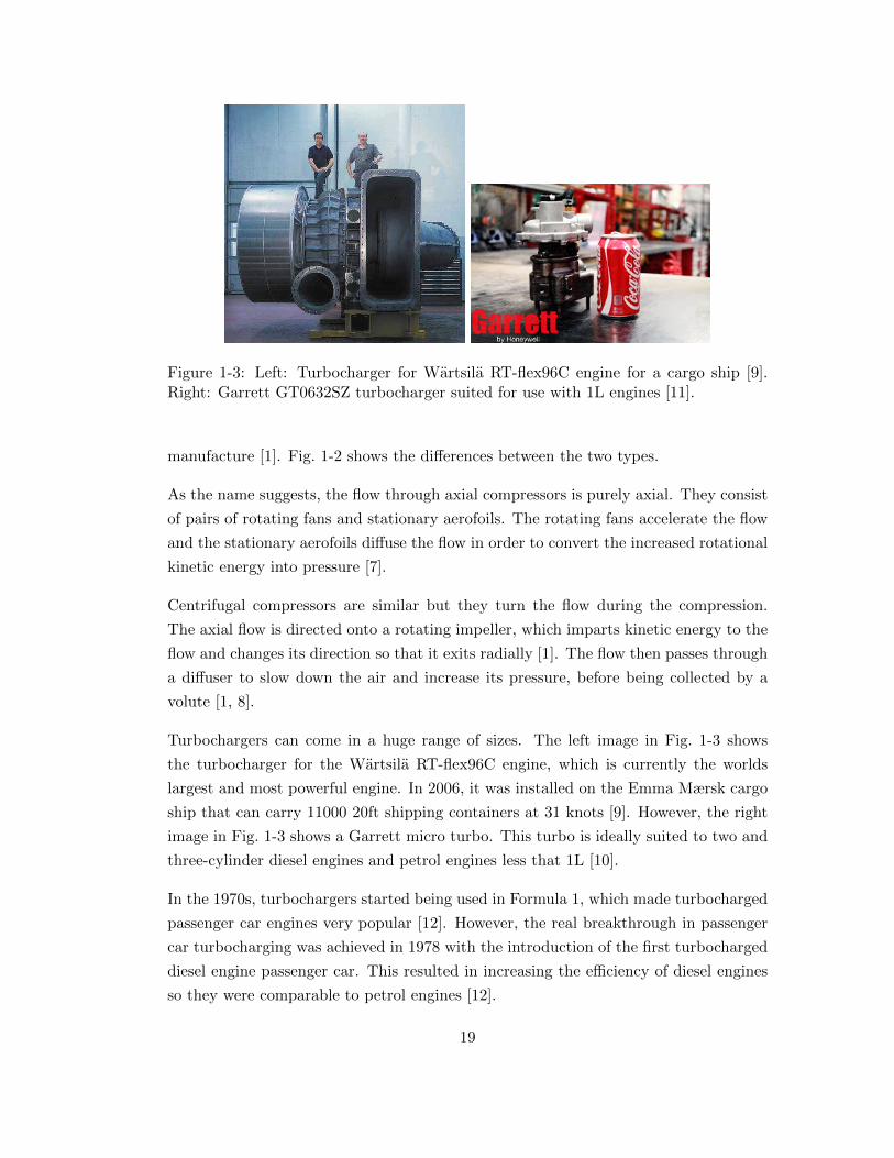
Figure 1-3: Left: Turbocharger for Wartsila RT-flex96C engine for a cargo ship [9].Right: Garrett GT0632SZ turbocharger suited for use with 1L engines [11].
manufacture [1]. Fig. 1-2 shows the differences between the two types.
As the name suggests, the flow through axial compressors is purely axial. They consist
of pairs of rotating fans and stationary aerofoils. The rotating fans accelerate the flow
and the stationary aerofoils diffuse the flow in order to convert the increased rotational
kinetic energy into pressure [7].
Centrifugal compressors are similar but they turn the flow during the compression.
The axial flow is directed onto a rotating impeller, which imparts kinetic energy to the
flow and changes its direction so that it exits radially [1]. The flow then passes through
a diffuser to slow down the air and increase its pressure, before being collected by a
volute [1, 8].
Turbochargers can come in a huge range of sizes. The left image in Fig. 1-3 shows
the turbocharger for the Wartsila RT-flex96C engine, which is currently the worlds
largest and most powerful engine. In 2006, it was installed on the Emma Mærsk cargo
ship that can carry 11000 20ft shipping containers at 31 knots [9]. However, the right
image in Fig. 1-3 shows a Garrett micro turbo. This turbo is ideally suited to two and
three-cylinder diesel engines and petrol engines less that 1L [10].
In the 1970s, turbochargers started being used in Formula 1, which made turbocharged
passenger car engines very popular [12]. However, the real breakthrough in passenger
car turbocharging was achieved in 1978 with the introduction of the first turbocharged
diesel engine passenger car. This resulted in increasing the efficiency of diesel engines
so they were comparable to petrol engines [12].
19
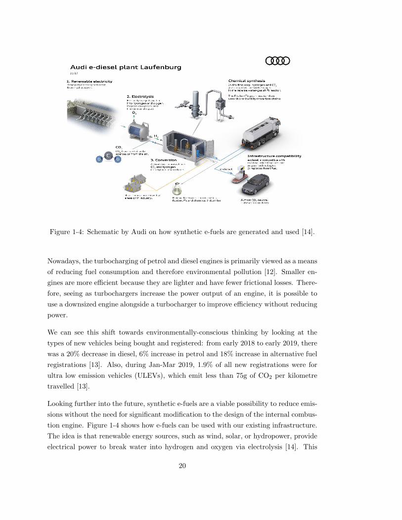
Figure 1-4: Schematic by Audi on how synthetic e-fuels are generated and used [14].
Nowadays, the turbocharging of petrol and diesel engines is primarily viewed as a means
of reducing fuel consumption and therefore environmental pollution [12]. Smaller en-
gines are more efficient because they are lighter and have fewer frictional losses. There-
fore, seeing as turbochargers increase the power output of an engine, it is possible to
use a downsized engine alongside a turbocharger to improve efficiency without reducing
power.
We can see this shift towards environmentally-conscious thinking by looking at the
types of new vehicles being bought and registered: from early 2018 to early 2019, there
was a 20% decrease in diesel, 6% increase in petrol and 18% increase in alternative fuel
registrations [13]. Also, during Jan-Mar 2019, 1.9% of all new registrations were for
ultra low emission vehicles (ULEVs), which emit less than 75g of CO2 per kilometre
travelled [13].
Looking further into the future, synthetic e-fuels are a viable possibility to reduce emis-
sions without the need for significant modification to the design of the internal combus-
tion engine. Figure 1-4 shows how e-fuels can be used with our existing infrastructure.
The idea is that renewable energy sources, such as wind, solar, or hydropower, provide
electrical power to break water into hydrogen and oxygen via electrolysis [14]. This
20

can then be combined with carbon dioxide to obtain e-methane, e-diesel, or e-kerosene.
Therefore, these fuels are having a net-zero carbon impact as they utilise carbon that
is already in the atmosphere, rather than adding carbon to the atmosphere that is
currently stored in the ground, e.g. through fossil fuels [14].
The fact that this would allow the internal combustion engine to remain relatively the
same, also means that turbochargers will still be useful in the future for improving
efficiency or power from an engine.
For this thesis, we will focus on automotive turbochargers. The automotive industry
is large and has been continually growing since the end of WWII. At the end of March
2019, there were 38.4 million vehicles licensed in Great Britain: 82.5% were cars, 10.6%
were LGVs, 1.3% were HGVs, and 3.3% were motorcycles [13]. Therefore, focusing on
improvements for automotive applications, particularly cars, has the potential for a
large impact.
Since the majority of cars use relatively small radial turbochargers, we will focus our
attention on these. However, the methodology discussed within this thesis can be used
for larger turbochargers and adapted for other applications.
1.1.2 Operation of Radial Compressors
Figure 1-5 shows the four components of a radial compressor: the inlet pipe, the
impeller, the diffuser and the volute.
The inlet is a simple pipe which directs the flow from above onto the impeller eye.
Some inlets have guide vanes in order to gain some control over the flow behaviour [1].
Figure 1-5: Components of a radial compressor from side and plan view points [15].
21
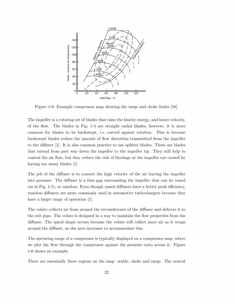
Figure 1-6: Example compressor map showing the surge and choke limits [16].
The impeller is a rotating set of blades that raise the kinetic energy, and hence velocity,
of the flow. The blades in Fig. 1-5 are straight radial blades, however, it is more
common for blades to be backswept, i.e. curved against rotation. This is because
backswept blades reduce the amount of flow distortion transmitted from the impeller
to the diffuser [1]. It is also common practice to use splitter blades. These are blades
that extend from part way down the impeller to the impeller tip. They still help to
control the air flow, but they reduce the risk of blockage at the impeller eye caused by
having too many blades [1].
The job of the diffuser is to convert the high velocity of the air leaving the impeller
into pressure. The diffuser is a thin gap surrounding the impeller that can be vaned
(as in Fig. 1-5), or vaneless. Even though vaned diffusers have a better peak efficiency,
vaneless diffusers are more commonly used in automotive turbochargers because they
have a larger range of operation [1].
The volute collects air from around the circumference of the diffuser and delivers it to
the exit pipe. The volute is designed in a way to maintain the flow properties from the
diffuser. The spiral shape occurs because the volute will collect more air as it wraps
around the diffuser, so the area increases to accommodate this.
The operating range of a compressor is typically displayed on a compressor map, where
we plot the flow through the compressor against the pressure ratio across it. Figure
1-6 shows an example.
There are essentially three regions on the map: stable, choke and surge. The central
22

stable area is the region of normal operation of the compressor. It is bounded on the
left by the surge line and on the right by a choking region.
The choking region is where the air velocity at some location within the compressor
approaches sonic conditions and so the compressor can’t accept any higher mass flow
rate. In this scenario, the compressor speed is likely to rise substantially with little
change to the mass flow rate [1].
The surge region is where flow instabilities are observed. The dividing line between
stable operation and surge is often difficult to predict as it depends on the whole
compression system, not just the compressor itself.
1.1.3 Surge and its Problems
Surge is an aerodynamic instability that exists when operating a compressor at low mass
flow rates. Normally air flows from regions of high pressure to regions of low pressure.
The compressor generates pressure in the outlet pipe and so the air is travelling against
the pressure gradient.
When operating with a small mass flow, it is possible for flow reversal to occur as the
force applied to the fluid by the pressure gradient is large enough to overcome the fluid
momentum. Once flow reversal occurs, the pressure drops in the outlet pipe and the
air resumes its forward directional flow. This oscillation in mass flow and pressure is
termed surge [1].
Surge is a large amplitude, low frequency oscillation of the averaged flow through the
compressor [17]. However, there are different classifications of surge.
When the oscillations in mass flow are large enough that actual flow reversal is seen,
this is called deep surge [18]. Alternatively, when mass flow and pressure oscillations
are observed but the flow always remains travelling in the forward direction, this is
classed as mild or incipient surge [18].
It is also possible to see a combination of behaviours. For example, Fig. 1-7 illustrates
an observable limit cycle for surge behaviour. It has four operating regimes: (1) The
speed of the flow at the impeller tip increases and the mass flow rate decreases; (2) The
compressor operates in mild surge, so fluctuations in pressure and mass flow grow; (3)
The mass flow reverses and the pressure drastically decreases; (4) The flow recovers
rapidly to the forward direction and the cycle repeats from (1) [19].
23

Figure 1-7: Time-resolved behaviour during a surge limit cycle, where ΦC denotesdimensionless mass flow in the compressor, and Ψ denotes dimensionless pressure [19].
Surge is commonly found to be triggered by some form of stall. There are two main
types of stall.
The first can occur at the inlet to the impeller or a vaned diffuser and is caused by
incidence. This means that, as mass flow decreases, the inlet flow angle increases and
causes a separation of the flow at the blade or vane wall [1].
The second type is often seen in a vaneless diffuser and is caused by recirculation. This
is where friction reduces the radial velocity of the flow near the shroud-side wall of the
diffuser, reducing its spiral angle so that it is swept back into the impeller [1].
It has been discovered that a compressor operating at high impeller speed is more likely
to surge due to stall in the diffuser, and a compressor operating at low impeller speed
is more likely to surge due to stall in the impeller inducer [20].
Operation in deep surge often damages the compressor and surrounding installation,
which can be costly to repair [1]. Surge causes vibrations that can unbalance the
machinery, which can result in contact between the impeller blades and the housing.
This leads to bending or fracture of the impeller blades. Operation in surge also results
in excessive internal temperatures due to extra friction between the components and
energy losses in the air as it recirculates. This rise in temperature can damage the
installation, for example through the melting of plastic connectors [17].
24

The mild form of surge is less damaging, but is still very noisy. This causes problems
with customer acceptance because the sound would be off-putting to any driver.
Since surge limits the amount of boost provided at low engine speeds, it is desirable
to operate close to surge without entering it for prolonged periods of time. Therefore,
it is important for designers and manufacturers to create models that can predict the
location of the surge region, as well as aid understanding of the flow dynamics near
that region.
However, due to the unstable nature of surge, and the fact that it depends on the
system pipework, this limit is often difficult to predict. Motivated by this, the work
undertaken in this thesis looks into new approaches for modelling and predicting surge
in radial compressors.
1.2 Literature Review
1.2.1 Existing Models
Models Requiring Turbochargers
There are many reasons why simulating an engine is useful. It allows for the prediction
of performance under different operating conditions, as well as optimisation and devel-
opment of designs of specific components. Therefore, even when turbochargers are not
the main focus of research, it is often important to have a model of them so the entire
engine performance can be studied.
There are many industrially-focused engine simulation software packages available, in-
cluding GT-POWER, Ricardo Wave, and LESoft [21, 22]. GT-POWER is part of
the GT-SUITE by Gamma Technologies. It is able to predict engine performance
quantities, like power and torque, and includes physical models for wave dynamics,
combustion and after-treatment [22].
Most of the systems being analysed are highly complex. For example, Fig. 1-8 shows
schematic of a 4-cylinder turbocharged engine modelled in GT-POWER. Each compo-
nent has its own model, so it is important that individual models are computationally
fast because running the whole system will call on each component multiple times.
This means that the current models for turbochargers in these engine systems are very
25
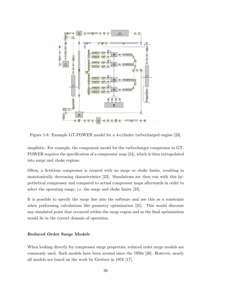
Figure 1-8: Example GT-POWER model for a 4-cylinder turbocharged engine [23].
simplistic. For example, the component model for the turbocharger compressor in GT-
POWER requires the specification of a compressor map [24], which is then extrapolated
into surge and choke regions.
Often, a fictitious compressor is created with no surge or choke limits, resulting in
monotonically decreasing characteristics [23]. Simulations are then run with this hy-
pothetical compressor and compared to actual compressor maps afterwards in order to
select the operating range, i.e. the surge and choke limits [23].
It is possible to specify the surge line into the software and use this as a constraint
when performing calculations like geometry optimisation [25]. This would discount
any simulated point that occurred within the surge region and so the final optimisation
would lie in the correct domain of operation.
Reduced Order Surge Models
When looking directly for compressor surge properties, reduced order surge models are
commonly used. Such models have been around since the 1950s [26]. However, nearly
all models are based on the work by Greitzer in 1976 [17].
26

Figure 1-9: Compression system used in Greitzer’s model [17]. The pipes containingthe compressor and throttle have much smaller diameters than the plenum, and havelengths Lc and LT respectively.
Greitzer simplifies an axial compression system to the model shown in Fig. 1-9. Here,
the compressor (modelled via an actuator disk) is connected to a large exit plenum,
and the air discharges through a throttle (also represented by an actuator disk) [17].
Greitzer considered flows of low inlet Mach number, so the associated pressure rise
is small in comparison to ambient pressure. This, combined with the relatively low
oscillation frequency of surge, meant Greitzer could assume the flow in the compressor
and throttle pipes was incompressible. The one dimensional incompressible momentum
equation is given by
ρdu
dt= −∂p
∂x. (1.2.1)
Integrating this with respect to x in the compressor and throttle pipes gives
LcAc
dmc
dt= ρcLc
ducdt
= pc − pp, (1.2.2)
LTAT
dmT
dt= ρTLT
duTdt
= pp − pT , (1.2.3)
where subscripts p, c and T denote the plenum, compressor and throttle respectively,
and m = Aρu is the mass flow rate with cross-sectional area, A. [17]
Greitzer assumed the plenum is large enough so that fluid velocities are negligible, but
still smaller than the wavelength of an acoustic wave oscillating at a typical surge fre-
quency. The latter assumption allowed Greitzer to also assume the pressure is constant
in space throughout the plenum at any instant in time. Applying conservation of mass
in the plenum gives us
mc − mT = Vpdρpdt
=ρambVpγpamb
dppdt, (1.2.4)
27

by assuming the fluid is isentropic and that temperature in the plenum Tp =ppRρp
is
ambient. Here Vp denotes the volume of the plenum and γ is the specific heat ratio.
[17]
Therefore, Greitzer is assuming that all of the kinetic energy of the flow is associated
with the motion of the fluid in the compressor and throttle pipes, and all of the potential
energy is associated with the compression of the gas in the plenum [17].
To close the system we need to know pc and pT . Greitzer decided to use
tdpcdt
= pcss − pc (1.2.5)
to determine pc, where pcss denotes a steady-state compressor characteristic, and t is a
time constant that describes the growth of stall cells (usually obtained via experiment).
Using this ODE instead of directly assuming pc ≈ pcss allows the model to simulate
the lag in compressor response, which can cause a lag between reaching the stall limit
and observing rotating stall cells or surge. [17]
For pT Greitzer assumed that we have either a variable area nozzle or a valve, so that
the orifice equation
pT =1
2ρambu
2T =
m2T
2ρambA2T
(1.2.6)
holds [17].
Greitzer then nondimensionalised the mass flows with ρambΩAc, the pressures with12ρambΩ
2 and the time variables with 1ωH
, where ωH = a√
AcVpLc
is the Helmholtz fre-
quency, Ω is the mean rotor velocity, and a is the speed of sound.
Denoting the dimensionless mass flows by Φ, the dimensionless pressure differences by
Ψ, and dimensionless time variables by τ , leads to the system
dΦc
dτ= B(Ψc −Ψ) (1.2.7)
dΦT
dτ=B
G(Ψ−ΨT ) (1.2.8)
dΨ
dτ=
1
B(Φc − ΦT ) (1.2.9)
dΨc
dτ=
1
τ(Ψcss −Ψc) (1.2.10)
where G = LTAcLcAT
, and B = Ω2a
√VpAcLc
[17]. B is often referred to as Greitzer’s parameter
28

and can be regarded as the ratio of pressure forces and inertial forces acting in the
compressor pipe [27].
Often, this system of ODEs is simplified further by assuming (i) τ = 0, so the com-
pressor acts in a quasi-steady manor, and (ii) that the pressure at the throttle is set
instantaneously by the pressure in the plenum so we can use
mT =√
2ρambA2T pp (1.2.11)
as a direct function instead of the ODE (see, for example, [28], [19], [29]). This would
reduce the above system to just two ODEs, namely:
dΦc
dτ= B(Ψcss −Ψ) (1.2.12)
dΨ
dτ=
1
B(Φc − ΦT ) (1.2.13)
where ΦT is the nondimensional form of the throttle equation. This system is often
referred to as the Moore-Greitzer equations.
Despite the fact Greitzer’s model was derived for axial compressors, this model has also
been used for radial compressors. For example, Arnulfi et al. [27] used a model derived
from Greitzer’s in order to simulate an industrial low-pressure multistage centrifugal
compressor with vaned diffusers. The main difference in Arnulfi’s model was the use
of a discontinuous parameter for τ so that a significant time lag was only introduced
when stalling occurred because this matched observed experiments [27].
Similarly, Elder et al. [20] and Fink et al. [19] used models based on Greitzer’s for vaned
and vaneless radial compressors respectively. However, instead of using experiments
to determine the compressor characteristic, they used meanline or lumped parame-
ter modelling approaches. Furthermore, Fink et al. extended Greitzer’s work to take
into account the effect of impeller inertia and speed variation, but this required the
additional specification of a torque characteristic [19].
There are many examples of these quasi-steady compressor models in literature, how-
ever, the main variation in the work seems to be how the compressor characteristic is
specified. The steady-state behaviour of the compressor is far more complex than that
of the throttle and so a characteristic is more complicated to determine. There have
been three main approaches for obtaining the compressor characteristics.
The first is through complex experimental studies. In 1984, Koff and Greitzer [30]
29
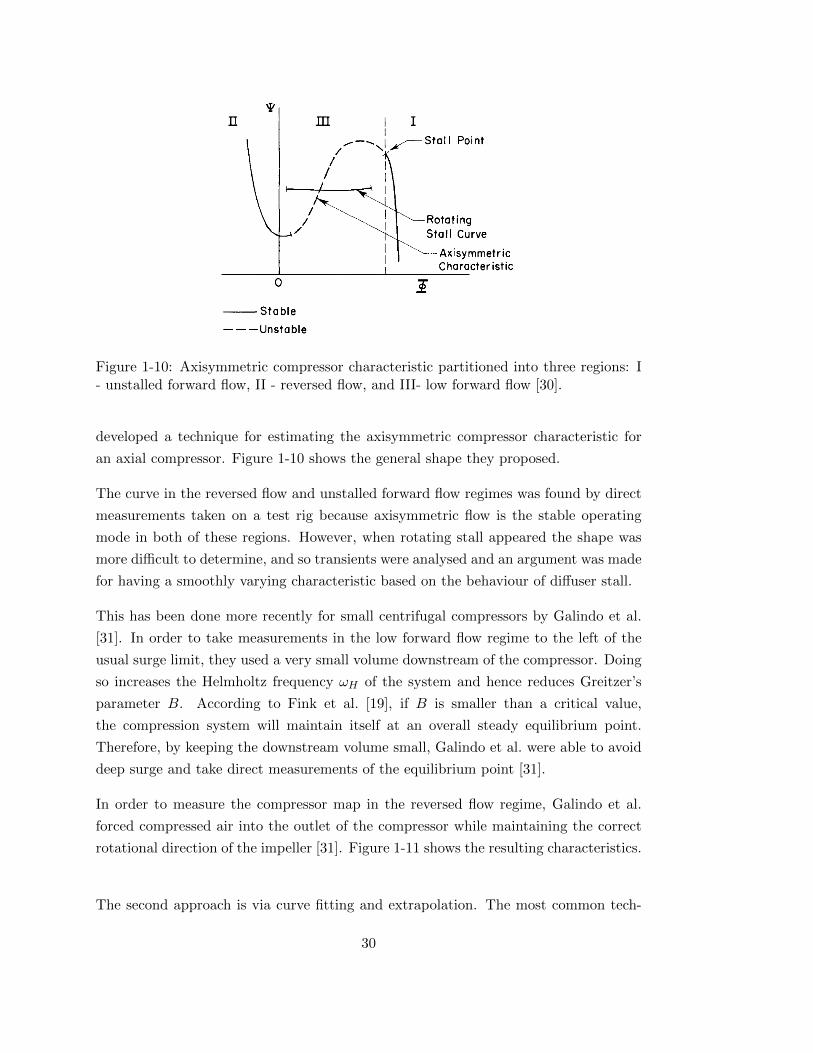
Figure 1-10: Axisymmetric compressor characteristic partitioned into three regions: I- unstalled forward flow, II - reversed flow, and III- low forward flow [30].
developed a technique for estimating the axisymmetric compressor characteristic for
an axial compressor. Figure 1-10 shows the general shape they proposed.
The curve in the reversed flow and unstalled forward flow regimes was found by direct
measurements taken on a test rig because axisymmetric flow is the stable operating
mode in both of these regions. However, when rotating stall appeared the shape was
more difficult to determine, and so transients were analysed and an argument was made
for having a smoothly varying characteristic based on the behaviour of diffuser stall.
This has been done more recently for small centrifugal compressors by Galindo et al.
[31]. In order to take measurements in the low forward flow regime to the left of the
usual surge limit, they used a very small volume downstream of the compressor. Doing
so increases the Helmholtz frequency ωH of the system and hence reduces Greitzer’s
parameter B. According to Fink et al. [19], if B is smaller than a critical value,
the compression system will maintain itself at an overall steady equilibrium point.
Therefore, by keeping the downstream volume small, Galindo et al. were able to avoid
deep surge and take direct measurements of the equilibrium point [31].
In order to measure the compressor map in the reversed flow regime, Galindo et al.
forced compressed air into the outlet of the compressor while maintaining the correct
rotational direction of the impeller [31]. Figure 1-11 shows the resulting characteristics.
The second approach is via curve fitting and extrapolation. The most common tech-
30

Figure 1-11: Measured steady-state compressor map extended into the surge and neg-ative flow zones experimentally [31].
nique is to use the cubic relation proposed by Moore and Greitzer in 1986 [32], i.e.
Ψcss = ψc0 +H
[1 +
2
3
(Φ
W− 1
)− 1
2
(Φ
W− 1
)3]
(1.2.14)
with parameters ψc0 , H and W found through fitting to experimental compressor map
data. However other curve fitting techniques have been proposed, including ones involv-
ing Chebyshev polynomials in order to capture more features of the characteristics [33],
and ones involving elliptic equations in order to adjust the characteristic for different
settings on a variable-geometry diffuser [34].
The third is via meanline modelling. In a mean-line model the compressor is divided
into sections over which the equations of motion and loss models are evaluated. Most of
the mean-line models follow the meridional path of the compressor and typically split
it into sections for the inlet, impeller, diffuser and volute [20, 35]. However, there are
two-zone models that have primary and secondary flow sections within the impeller in
order to account for slip [36].
The majority of these mean-line models apply empirical loss models to the sections.
Typical collections of loss models for compressors can be found in [37, 38, 39]. These
loss models usually have loss coefficients that need to be tuned to the particular com-
pressor that is being studied, which makes meanline modelling still partially reliant on
experimental data or CFD simulation.
31
Computational Fluid Dynamics
When more detailed modelling of a turbocharger is required, engineers typically turn to
numerical simulation software like Ansys-CFX to perform computational fluid dynamics
(CFD). With the advancement in computing power, this has been a growing area of
interest.
In a CFD model, a 3D domain is built in the computer and a mesh is constructed over
it. This mesh divides the domain into millions of control volumes, or cells, within which
the conservation of mass, momentum and energy equations can be solved numerically
using finite differences (FDs) or finite element methods (FEMs) [40].
FEM uses the weak form of the equations of motion. To exemplify this, consider the
1D Poisson’s equation
−d2w
dx2= g, w(±1) = 0. (1.2.15)
The weak form is found by multiplying by an arbitrary function v such that v(±1) = 0
and integrating [41]. So we get
∫ 1
−1vgdx = −
∫ 1
−1vd2w
dx2dx =
>
0
−vdwdx
∣∣∣∣1
−1
+
∫ 1
−1
dv
dx
dw
dxdx. (1.2.16)
From here, we define a finite dimensional basis, φ1, φ2, ..., φn, where each function
satisfies the boundary condition φi(±1) = 0, ∀i. We can then find an approximate
solution to w via w ≈∑ni=1wiφi, which will converge to the exact solution as n→∞
[41]. Writing v =∑n
j=1 vjφj we get
n∑
j=1
vj
∫ 1
−1φjgdx =
n∑
j=1
n∑
i=1
vj
(∫ 1
−1
dφjdx
dφidx
dx
)wi, (1.2.17)
which in vector notation becomes vT c = vTKw where
cj =
∫ 1
−1φjgdx and Kji =
∫ 1
−1
dφjdx
dφidx
dx. (1.2.18)
Therefore, this just reduces to the matrix solve of Kw = c to find the vector of
coefficients for the approximate solution w.
The simplest basis for FEM are piecewise linear functions φi(xj) = δij where δij is the
32

Figure 1-12: Example FEM basis with piecewise linear functions φ2(x) and φ3(x) shownwith solid and dashed lines respectively [41]. Each function φi will only interact withits two neighbours.
Kronecker delta (see Fig. 1-12). This means that
cj =
∫ 1
−1φjgdx ≈
n∑
i=1
δijg(xi) = g(xj) (1.2.19)
so the function only needs to be known at the grid points, x1, x2, ..., and we have a
summation over evaluated function points.
This basis has the advantage that K will be tridiagonal, hence the system Kw = c
can be solved very quickly, however convergence to the true solution can be slow and
so often a large n is required for accuracy [41].
Automatic, CFD based geometric optimisations are commonly used by centrifugal com-
pressor designers. However, one major issue that remains unresolved is how to deter-
mine the surge margin of these compressors [42].
Conducting a detailed, fully-unsteady, 3D flow analysis through a compressible large-
eddy simulation would be the most appropriate method for determining the surge
limit. However, since the impeller runs at speeds requiring thousands of revolutions
per second and surge has a period of approximately 0.1 seconds, many iterations of
the CFD model are needed to simulate a single surge cycle. Furthermore, a fine mesh
would be required in order to capture the small scale flow dynamics, like impeller stall,
that influence surge, so this is far too computationally expensive for manufacturing
needs [42].
Therefore, a common method is to run a steady-state CFD simulation iteratively along
a speed line, and define the surge limit as the last converged CFD calculation [42]. This
is not ideal as there could be other reasons why a simulation did not converge, and the
need for multiple iterations still makes this method costly in terms of computation.
Furthermore, running a complex CFD model often doesn’t have the ability to identify
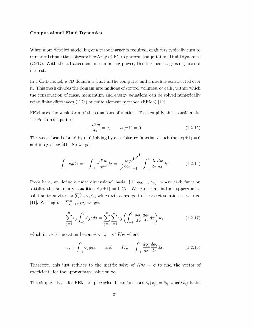
33
Figure 1-13: Lagrange polynomial basis [41]. (a) Global basis for SM method, withφ2 (solid) and φ4 (dashed). (b) Local basis for SEM method, with φ2 (solid) and φ3
(dashed).
key parameters of physical phenomena that lead to certain events. For example, by
defining the surge limit to be the last converged CFD simulation, it is not simple to
identify from previous simulations what physical phenomena are contributing to surge
because there are many variables and interactions to consider.
1.2.2 Alternative Modelling Techniques
Further to the existing compressor and surge related models, there are other mathe-
matical modelling techniques that could be helpful for analysing surge.
Advanced Numerical Approaches
Numerical methods for simulating flows are becoming increasingly common. One such
area of interest are Spectral Methods (SMs) and Spectral Element Methods (SEMs).
These work in a similar way to the FEM described above. They also require a weak
form of the problem, and expand the solution in terms of a basis [41]. The key difference
is in the choice of basis. While FEM resulted in a summation of evaluated function
values, SMs and SEMs approximate a solution as a summation of functions.
SMs are those where each function in the basis spans the entire domain (i.e. a global
basis) whereas SEMs are similar to the FEM in that they are only non-zero over
a small portion of the domain (i.e. a local basis) [41]. Common basis choices for
SMs are trigonometric functions (see [43] for example), or Lagrange polynomials [41].
Restricting Lagrange polynomials to certain parts of the domain would result in a SEM.
Figure 1-13 shows Lagrange polynomials as a global basis and a local basis.
Since SMs require a basis that is defined over the entire domain while still satisfying
34
the boundary conditions, these methods are only suitable when the domain comprises
of simple geometries. For more complicated geometries, SEMs are needed.
The choice of the basis functions is important when considering computational cost.
Not only will a large basis (i.e. n 1) increase computational cost, but a poorly
conditioned matrix K will also cause these methods to be costly [41].
SMs and SEMs have been used for solving the Navier-Stokes fluid equations. For ex-
ample, Lomtev and Karniadakis [44] develop a discontinuous spectral method with a
hierarchical basis formed from Jacobi polynomials. This formulation sees good conver-
gence even on a highly distorted mesh, and high computational efficiency [44]. There-
fore, it would be possible to extend works like this to improve the efficiency of CFD
codes used for simulating compressor surge.
Statistical Approaches
Another mathematical approach to consider is statistical regression modelling. This
is where experimental data is used to predict how a variable is dependent on other
known parameters. So, in the context of surge, we could find a statistical model for
the location of the surge limit by considering geometric dimensions of the compressor
and test rig, and operating parameters like impeller speed. This approach could also
be used to create a function for the compressor characteristic that depends on known
geometry.
One such approach is to fit a Generalised Additive Model (GAM). Suppose that we
want to estimate a formula for the random variable Wi and we have a set of observed
data wi along with known parameters v1i, v2i, v3i, ... then a GAM takes the form
g0(E(Wi)) = g1(v1i) + g2(v2i) + g3(v3i) + ... (1.2.20)
for functions gi, where E is the expectation over many realisations of the variable at
fixed parameter values [45]. We can find the best fit for the functions gi by expanding
them in terms of a basis. For example, suppose we wish to understand how the wear
of a car engine depends on its size. Labelling wi = wear and vi = size, means we wish
to fit the GAM:
wi = g(vi) + εi, (1.2.21)
35

Figure 1-14: GAM fit of engine wear vs size for a basis of size k = 6 [45].
where ε represents noise in the observed data. To find g we can write
g(x) =k∑
j−1
φj(x)ϑj , (1.2.22)
where φj are basis functions, and ϑj are unknown parameters that we can find via a
least squares fit to the observed data [45]. For this example with a piecewise linear
basis for size k = 6 we get the resulting function in Fig. 1-14.
Choosing the basis size k automatically from the data is difficult, so instead k is usually
set to equal the number of data points and
||w − V ϑ||+ λsϑTSϑ (1.2.23)
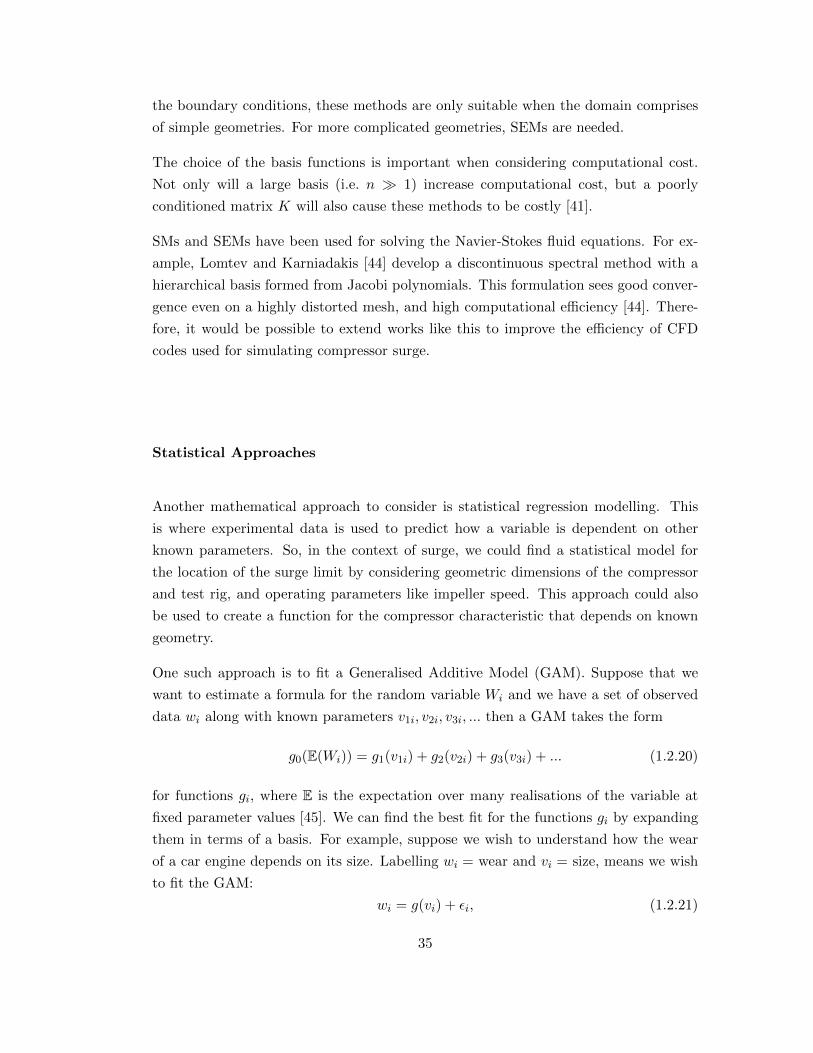
is minimised to penalise the sinuousness of the fitting [45]. Here, ϑTSϑ are the squared
differences and λs is referred to as the smoothing parameter. This is determined by
minimising the Generalised Cross Validation (GCV), which is a measure of how well
the fitted function approximates each data point in turn [45]. The resulting GAM fit
for this is shown in Fig. 1-15
As can be seen, even simple piecewise linear GAM fits can produce reasonable models
for estimating a variable. The main downside to statistical approaches is the require-
ment of a large amount of data that spans the parameters of interest. For example, for
surge we would need test data for different types and sizes of turbochargers, as well as
different rigs and operating conditions.
36
Figure 1-15: Left: Generalised Cross Validation score used to identify smoothing pa-rameter λ ≡ λs [45]. Right: GAM fit of engine wear vs size for this smoothing parameter[45].
Reduced Modelling
Finally, we will discuss reduced modelling approaches. These are techniques where we
reduce the complexity (usually via reduction in the dimension) of the problem but still
retain the dominant behaviours in the solution. There are numerous approaches that
fit in this category; some follow formal procedures and others have a more flexible,
ad-hoc method.
One approach is called averaging. As the name suggests, this is where we replace the
original functions of the system with the average over one or more dimensions.
Averaging over time is commonly used in dynamical systems to give asymptotic ap-
proximations to the original time-dependent system [46]. For example, suppose we
have a periodic system dependent on some small parameter ε,
x = εg(x, t, ε), g(x, t, ε) = g(x, t+ T, ε). (1.2.24)
Since ε is small, the change in x with time is slow in comparison to the period of oscil-
lation T . Often we are interested in the overall dynamic behaviour and less interested
in the small fluctuations with time. Therefore, we can compute the time average of the
function g by
g(x) =1
T
∫ T
0g(x, s, 0) ds. (1.2.25)
It has been shown that the solution w to w = εg(w) will be within O(ε) of the true
37
solution x(t) for t < 1ε , so we can use w to give us insight to the overall dynamic
behaviour of the system [46].
It is possible to use averaging with systematic asymptotic methods in order to capture
more of the solution complexity. For example, suppose we have flow down a straight
pipe in the x direction, then the average flows in the y and z directions would be zero.
We could write the flow velocity as
u(t, x, y, z) = u(t, x)ex + u(t, x, y, z), (1.2.26)
where u is the deviation of the flow from the average flow. This deviation is likely to be
largest at the pipe walls, and so Boundary Layer Theory (see for example [47]) could
be applied to understand more of the flow dynamics and help quantify the error of the
averaging approximation.
Another reduced modelling approach is Galerkin truncations. This is where variables
are expanded in terms of basis functions. That way, model reduction can be achieved
by selecting the first few dominant terms.
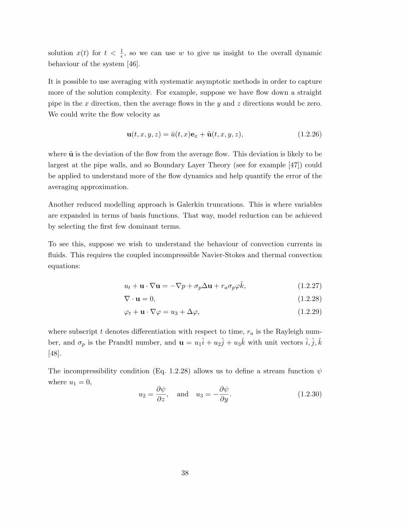
To see this, suppose we wish to understand the behaviour of convection currents in
fluids. This requires the coupled incompressible Navier-Stokes and thermal convection
equations:
ut + u · ∇u = −∇p+ σp∆u + raσpϕk, (1.2.27)
∇ · u = 0, (1.2.28)
ϕt + u · ∇ϕ = u3 + ∆ϕ, (1.2.29)
where subscript t denotes differentiation with respect to time, ra is the Rayleigh num-
ber, and σp is the Prandtl number, and u = u1i + u2j + u3k with unit vectors i, j, k
[48].
The incompressibility condition (Eq. 1.2.28) allows us to define a stream function ψ
where u1 = 0,
u2 =∂ψ
∂z, and u3 = −∂ψ
∂y. (1.2.30)
38
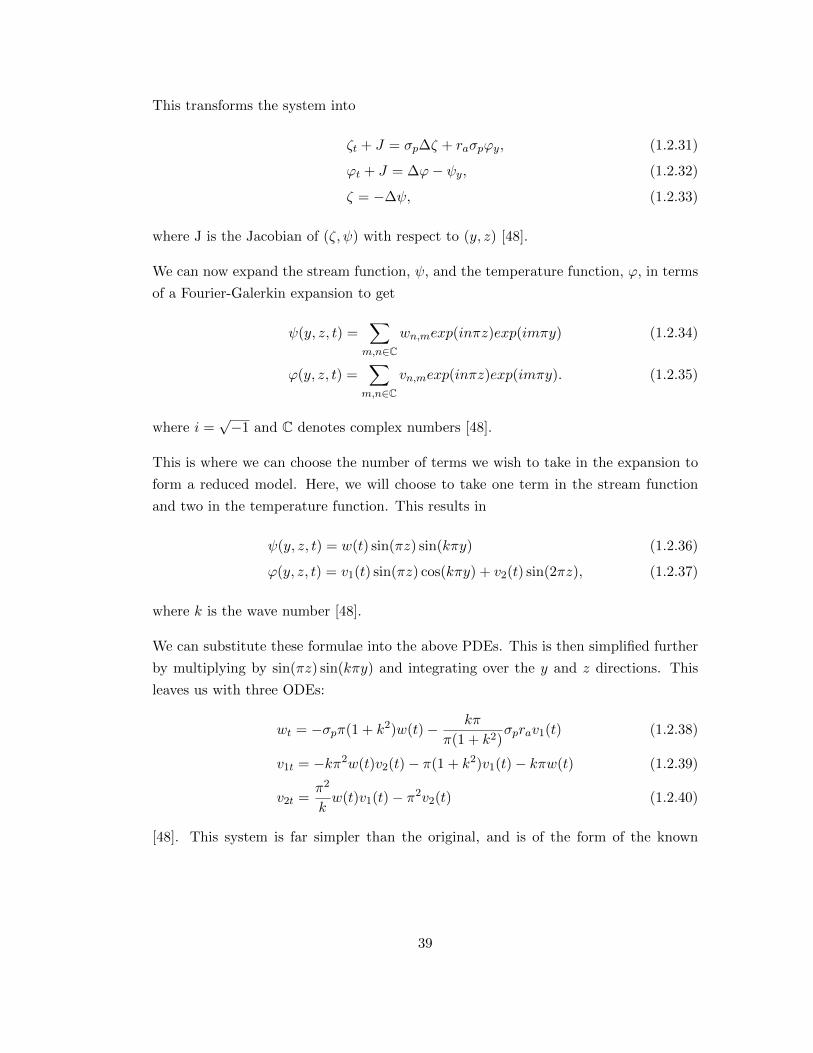
This transforms the system into
ζt + J = σp∆ζ + raσpϕy, (1.2.31)
ϕt + J = ∆ϕ− ψy, (1.2.32)
ζ = −∆ψ, (1.2.33)
where J is the Jacobian of (ζ, ψ) with respect to (y, z) [48].
We can now expand the stream function, ψ, and the temperature function, ϕ, in terms
of a Fourier-Galerkin expansion to get
ψ(y, z, t) =∑
m,n∈Cwn,mexp(inπz)exp(imπy) (1.2.34)
ϕ(y, z, t) =∑
m,n∈Cvn,mexp(inπz)exp(imπy). (1.2.35)
where i =√−1 and C denotes complex numbers [48].
This is where we can choose the number of terms we wish to take in the expansion to
form a reduced model. Here, we will choose to take one term in the stream function
and two in the temperature function. This results in
ψ(y, z, t) = w(t) sin(πz) sin(kπy) (1.2.36)
ϕ(y, z, t) = v1(t) sin(πz) cos(kπy) + v2(t) sin(2πz), (1.2.37)
where k is the wave number [48].
We can substitute these formulae into the above PDEs. This is then simplified further
by multiplying by sin(πz) sin(kπy) and integrating over the y and z directions. This
leaves us with three ODEs:
wt = −σpπ(1 + k2)w(t)− kπ
π(1 + k2)σprav1(t) (1.2.38)
v1t = −kπ2w(t)v2(t)− π(1 + k2)v1(t)− kπw(t) (1.2.39)
v2t =π2
kw(t)v1(t)− π2v2(t) (1.2.40)
[48]. This system is far simpler than the original, and is of the form of the known
39
Lorenz system:
Xt = c1(Y −X) (1.2.41)
Yt = −Y + c2X −XZ (1.2.42)
Zt = −c3Z +XY, (1.2.43)
for constants ci, which has been frequently studied via dynamical systems analysis as
it is known to exhibit chaotic behaviour [48]. Therefore, it is possible to gain under-
standing of convection currents in fluids by studying the far simpler Lorenz equations.
1.2.3 Discussion of Approaches
Numerical
The accuracy of numerical simulations of flows has increased dramatically over the past
decade due to the rapid growth in high speed computing power. Spectral, or spectral
element, methods may be more computationally efficient than standard CFD codes,
but they are both typically run on high-performance super computers with parallel
code in order to achieve maximum accuracy in the shortest amount of time.
Since surge cycles often experience local or small scale phenomena like rotating stall, re-
circulation, and eddy currents, full unsteady 3D simulations are required to completely
capture the dynamics. CFD can struggle when modelling large scale phenomena that
depend on small scale effects because it is too computationally expensive to perform
this direct numerical simulation with the required fineness of mesh [40]. SM or SEM
methods with a hierarchical basis are better able to deal with different scales within
the simulation, so it is possible to use these methods for improvements to numerical
surge simulation.
However, CFD is a well established tool and so new numerical models are unlikely to
be taken up by companies. The industry is more likely to make use of less accurate
but very quick models that can help give insight into the behaviour of surge during the
early design stages, as they currently tend to rely heavily on experiments for this.
40

Experimental or Statistical
The advantage of using a predominantly experimental approach for surge studies is
its simplicity because reading data or evaluating polynomial-like expressions are very
quick computationally. However, surge is not always easy to measure experimentally.
This is partially due to its damaging nature, which means a compressor cannot be
operated in this region for long periods of time, and partially its complexity. For
example, sometimes the surge limit can be recorded at different locations for the same
experimental set-up, meaning it can be very sensitive to initial conditions.
Also, since surge is a system level phenomenon, the experimental results are often lim-
ited to the particular experimental set-up and not any compressor installation. This
means that a large variety of tests would need to be performed in order to understand
what behaviour is specific to that set-up and what can be applied universally. Conduct-
ing experiments are expensive in both equipment and time requirements; so approaches
that require a large amount of experimental data are less desirable [49].
Furthermore, forming functions based mostly on experiment makes it difficult to gain
intuition into why the system behaves as it does. This information is vital because if
we can understand what causes the system to surge, it can help control the system to
prevent it from occurring.
Reduced Modelling
Since numerical modelling would be too computationally expensive, and experimental
data doesn’t give us the required insight into the surge phenomenon, creating a reduced
model appears to be the best way forward.
Of the methods discussed in the previous section, averaging is the approach that is
easiest to compare back to the original physics. This not only makes any resulting
simulations easier to understand but gives us the freedom to incorporate some empiri-
cally generated physical models into the system. Furthermore, it is possible to extend
this approach at a later date to include asymptotics or Galerkin truncations on the
perturbation from the average flow.
The strength of having a mathematically simple model is that it is relatively simple to
perform analysis like stability analysis and bifurcation theory (see [28] for an example
of this analysis applied to Greitzer’s model). These are powerful tools which would
41

allow us to gain insight into how the dynamics of surge changes when parameters, such
as geometrical dimensions, are varied.
To model surge in a compression system, we could average the Navier-Stokes equations
for fluid motion in order to reduce the dimension from 3D in space to just 1D in space.
Doing this in a way that minimises the number of fitted parameters, would result in a
model with a high predictive ability.
Fast running, simple models that can predict the onset of surge for any turbocharger
and test rig set up would hugely benefit the turbocharger industry. It would speed up
the early design stages, due to less reliance on time consuming CFD, and reduce costs
because of a reduced need for experimental testing.
Greitzer’s model falls into this category of reduced models as it has integrated out the
spatial dependence, making it only dependant on time. The use of Greitzer’s model
in this from has been relatively unchanged over the past 30 years. Therefore, using
more analytical methods to develop a model similar to Greitzer’s could provide some
improvements.
Firstly, the derivation of Greitzer’s model relied on the specific set up of a test rig. In
particular, it required that the system contained a large exit plenum. However, a lot of
systems do not include such a plenum, so using the averaging technique on the specific
test rig or engine set up could improve accuracy of the model results.
Also, Greitzer’s ODEs are simplified ODEs with nonlinearity only appearing through
the assumed compressor and throttle characteristics. In contrast, by applying averaging
methods to the nonlinear Navier Stokes equations we could systematically retain all
required nonlinear terms and thus generate more accurate simulations.
Moreover, if we average to reduce the unsteady Navier Stokes equations from 3D to
1D spatially, we could evaluate the resulting PDE of time and space to simulate the
pressure and mass flow waves travelling through the system pipework. How these
waves interact with, say, their reflections, could provide some useful understanding of
the system level surge phenomena. Also, the PDE system being only 1D in space would
still run very quickly in comparison to CFD.
It is also important to note that systems like Greitzer’s rely on the specification of a
steady-state compressor characteristic. We could create a reduced model for this by
also using the technique of averaging on the steady Navier Stokes equations to reduce
the system to 1D in space. The benefit of using the same mathematical technique for
42

both parts of the surge model is that we would have consistency of assumptions with
both models.
Also, a reduced model for the compressor characteristic that is 1D in space would pro-
vide more detail than the meanline modelling approach. It would allow for simulation
of the steady-state flow throughout the compressor, rather than at the specific regions
that a meanline models evaluate over. Furthermore, as it would be developed directly
from the Navier Stokes equations, it can be created in a way that reduces the amount
of dependence on empirical loss models which would improve its predictive capability
and remove the need to tune the characteristic to a particular compressor.
1.3 Aims of Thesis
This thesis aims to:
Create a predictive model for the onset of compressor surge.
This model will need to balance the model accuracy with computational efficiency.
Therefore, we aim to develop a model that is as simple as possible, while still
capturing the main dynamics of surge.
Gain further understanding of surge dynamics.
This includes understanding the routes into surge, the pressure wave dynamics in
the compression system, and the stability of the system. Insight will be obtained
from both the development of, and the analysis of, any reduced order surge
models.
1.4 Structure of Thesis
Chapter 2 describes the initial formulation for a reduced order model for surge. It begins
by understanding the fundamental equations of fluid motion, and then uses averaging
techniques to develop a model to capture surge in a simple compression system.
The resulting model depends on the specification of compressor and throttle character-
istics. Therefore, equations for these are developed, again using averaging techniques
on the fundamental fluid equations.
43
Special care is taken during the creation of the compressor characteristic to ensure
that only the most essential dynamics are included. Thus keeping the characteristic as
computationally efficient as possible, but retaining the ability to capture all relevant
surge dynamics.
Chapter 3 takes a more detailed look into the dynamics of the system when the flow
in the compressor is reversed. The compressor characteristic is altered to ensure it
captures the reserve flow dynamics correctly, and is validated via experiments.
Chapter 4 extends the model for the compressor characteristic to allow the reduced
order surge model to capture both mild and deep surge oscillations. Also, the surge
model is studied in its PDE form and solved numerically in order to simulate mass
flow and pressure waves travelling through the system. The generated simulations are
validated through experimental surge tests.
Chapter 5 performs stability analysis on the ODE form of the reduced order surge
model. Linear stability analysis is used to determine what variables influence the loca-
tion of the surge limit, and bifurcation theory is used to explain some of the dynamics
observed in model simulations and experimental data.
Finally, Chapter 6 summaries the work undertaken in this thesis. It highlights the key
insights into the physics behind the surge phenomenon gained during the development
and analysis of the surge models. Suggestions for how this research could be extended
in the future are also made.
This thesis follows the alternative thesis format and so Chapters 2, 3, and 4 contain
papers that are published or submitted for publication.
44
Chapter 2
Reduced Model for Surge with
Cubic-shaped Compressor
Characteristics
Following from the discussion in Chapter 1, we shall address the thesis aims via the
creation of a new reduced order model for compressor surge. We shall develop this
by performing averaging techniques on the fundamental equations for fluid motion.
Starting from these fundamental equations allows us to keep track of any assumptions
being made, and ensure they are consistent throughout the model development.
2.1 Equations of Fluid Motion
There are three fundamental fluid equations that come from conservation laws. Namely,
conservation of mass, momentum and energy. In this section, we will derive these
equations so that we can gain a physical understanding of the individual terms.
2.1.1 Conservation of Mass
Consider a volume V (t) of fluid moving with time. The mass of this volume is given
by
m(t) =
∫
V (t)ρ dV (2.1.1)
45

where ρ is the density [50]. Since V (t) is a closed system and matter cannot be created
or destroyed, m(t) is constant in time, i.e.
dm
dt=
d
dt
∫
V (t)ρ dV = 0. (2.1.2)
We can use the Reynolds’ Transport Theorem to take the differential through the
integral sign. This gives us
∫
V (t)
∂ρ
∂t+∇ · (ρu) dV = 0. (2.1.3)
The first term is the change in mass with time within the volume V (t), and the second
is the mass flux into and out of the volume.
Since V (t) is a arbitrary volume of fluid, this implies that the integrand must be zero.
Hence, the conservation of mass can be written as
∂ρ
∂t+∇ · (ρu) = 0. (2.1.4)
2.1.2 Conservation of Momentum (in a Rotating Frame)
Suppose that we have a continuum of fluid with velocity u(x, t) = (u1(x, t), u2(x, t), u3(x, t))T ,
density ρ(x, t) and volume V (x, t), where x = (x1, x2, x3)T denotes position. The rate
of change of a quantity of interest, say g(x, t), as we follow the fluid is given by
Dg
Dt=∂g
∂t+
3∑
i=1
∂g
∂xi
dxidt
=∂g
∂t+ (u · ∇)g (2.1.5)
where DDt is termed the total derivative [51].
Now, Newton’s Second Law of motion states that the total force acting on a system
is equal to its mass multiplied by its acceleration. Since mass m = ρV , we can divide
through by volume to get
ρDu
Dt= F (2.1.6)
where F is the force acting on fluid per unit volume [52].
By expanding the total derivative, adding conservation of mass (Eq. 2.1.4) multiplied
46

by u, and noticing
(ρu · ∇)u + u∇ · (ρu) = ∇ · (ρ(u⊗ u)), (2.1.7)
Eq. 2.1.6 becomes∂
∂t(ρu) +∇ · (ρ(u⊗ u)) = F. (2.1.8)
This is now in a similar form to the conservation of mass, where the first term is the
change of momentum within the volume V and the second is the flux of momentum.
To find F, we need to consider three types of forces acting on the fluid: (i) gravitational,
(ii) internal stresses, and (iii) rotational.
For (i), Newton’s second law tells us the force applied to the fluid will be mg, where g
is acceleration due to gravity. Therefore, on division by volume, F(i) = ρg.
For (ii), note that the force applied to the fluid is a stress, Π, acting on an area. Using
the Divergence theorem, this becomes
∫
AΠ · dA =
∫
V∇ ·Π dV, (2.1.9)
and so the force per unit volume is F(ii) = ∇·Π. It is normal to decompose the stresses
into normal stresses (i.e. pressures) and shear stresses. Hence, Πij = −pδij + τij where
δij is the Kronecker delta and τ is the deviatoric stress tensor, and so F(ii) = −∇p+∇·τ[53].
Finally, for (iii), suppose that a particle of fluid is in a rotating field of angular velocity
Ω. Let S denote the stationary frame and R the rotating frame of reference. Then
if the particle moved in the rotating frame, an observer in stationary frame would see
this motion of the particle as well as the motion of the field. So if the particle has
position x, then (dx
dt
)
S
=
(dx
dt
)
R
+ Ω× x (2.1.10)
[54]. Differentiating this again, and noticing d2xdt2
= DuDt , gives us
(Du
Dt
)
S
=
(Du
Dt
)
R
+dΩ
dt× x + 2Ω× u + Ω× (Ω× x) (2.1.11)
[50]. Therefore, assuming the angular velocity is constant, Newton’s second law gives
us
F = ρ
(Du
Dt
)
R
= ρ
(Du
Dt
)
S
− 2ρΩ× u− ρΩ× (Ω× x). (2.1.12)
47

This means that the momentum in the rotating frame has two extra forces, F(iii) =
−2ρΩ× u− ρΩ× (Ω× x), than if the flow field was stationary. The term 2ρΩ× u is
called the Coriolis force and ρΩ× (Ω× x) is called the centrifugal force [51].
Putting all these together, we get that
F = ρg −∇p+∇ · τ − 2ρ(Ω× u)− ρ(Ω× (Ω× x)) (2.1.13)
is the total force acting on fluid per unit volume. Thus, the conservation of momentum
in a rotating frame becomes
∂
∂t(ρu) +∇ · (ρ(u⊗ u)) + 2ρ(Ω× u) + ρ(Ω× (Ω× x)) = ρg −∇p+∇ · τ . (2.1.14)
2.1.3 Conservation of Energy
The first law of thermodynamics states that
DQ
Dt=DU
Dt+DW
Dt, (2.1.15)
where Q is the heat energy supplied, U is the internal energy and DWDt is the work done
by the system.
There are two ways in which work is done on the fluid. The first is pressure causing a
change in volume, i.e.
pD
Dt
(1
ρ
). (2.1.16)
This can be written as pρ∇ · u because conservation of mass in total derivative form
gives usDρ
Dt= −ρ(∇ · u). (2.1.17)
The second is the work done on adjacent layers of a fluid by the action of shear forces
[55], i.e.
1
ρτ : ∇u =
1
ρ
3∑
i=1
3∑
j=1
τij∂ui∂xj
. (2.1.18)
Therefore, on multiplication by ρ, the equation for thermal energy is given by
ρDQ
Dt= ρ
DU
Dt+ p∇ · u− τ : ∇u. (2.1.19)
48
Now, taking the dot product of u with the conservation of momentum (Eq. 2.1.6 with
2.1.13) results in
ρu · Du
Dt= ρu · g− u · ∇p+ u · (∇ · τ )− 2ρu · (Ω× u)− ρu · (Ω× (Ω× x)). (2.1.20)
Notice that, u · (Ω× u) = 0,
u · (Ω× (Ω× x)) = −(Ω× x) · (Ω× u) = − D
Dt
( |Ω× x|22
), (2.1.21)
and
u · g = −D(gh)
Dt, (2.1.22)
where h is vertical height as u · g is the component of velocity acting in the direction
of gravity [52]. Therefore, we can write Eq. 2.1.20 in terms of total derivatives by
ρD
Dt
( |u|22
+ gh− |Ω× x|22
)= −u · ∇p+ u · (∇ · τ ). (2.1.23)
Finally, since −u · ∇p = p(∇ · u)−∇ · (pu), we have that
p(∇ · u) = ρD
Dt
( |u|22
+ gh− |Ω× x|22
)+∇ · (pu)− u · (∇ · τ ). (2.1.24)
Combining this with Eq. (2.1.19), and using u · (∇ · τ ) + τ : ∇u = ∇ · (τ · u), we get
ρDQ
Dt= ρ
D
Dt
( |u|22
+ gh− |Ω× x|22
+ U
)+∇ · (pu)−∇ · (τ · u). (2.1.25)
Define E to be the total specific energy in a rotating frame, i.e.
E =|u|2
2+ gh+ U − |Ω× x|2
2. (2.1.26)
Then, the conservation of energy becomes
ρDE
Dt+∇ · (pu)−∇ · (τ · u) = ρQ, (2.1.27)
or, on expansion of the total derivative and addition of conservation of mass (Eq. 2.1.4)
multiplied by E,
∂
∂t(ρE) +∇ · (ρuE + pu)−∇ · (τ · u) = ρQ. (2.1.28)
49
2.1.4 Initial Assumptions
Since we are looking in particular at air flow, we can make some initial assumptions.
Firstly, we will assume that we have a perfect gas, so U = cvT for a constant cv, and
an ideal gas so
p = ρRT. (2.1.29)
We can also assume that gravitational effects are negligible, because air density is
relatively small and we are assuming our turbochargers are not too far off the ground.
Finally, for the sake of model simplicity, we will assume we have no heat transfer and
no viscous dissipation, i.e. the terms Q and ∇ · (τ · u) are neglected. However, we will
still consider dissipative losses like friction.
2.2 Reduced Model for Surge
The next step in modelling surge is to apply the fundamental equations of fluid motion
to a situation where we know surge is observed.
In order to find the surge limit for turbochargers experimentally, they are usually in-
stalled on a gas stand where the compressor and turbine sections are independently
controlled. Different amounts of hot, compressed air can be fed into the turbine sec-
tion to set the rotor speed to a desired value. Figure 2-1 shows the compressor-side
installation, where the compressor is connected to a valve via a simple pipe. As the
valve is shut, the amount of air going through the compressor is restricted and surge
can be observed.
Let us model the air in the pipe between the compressor and throttle valve. The
equations of motion give us:
∂ρ
∂t+∇ · (ρu) = 0, (2.2.1)
∂
∂t(ρu) +∇ · (ρ(u⊗ u)) = −∇p+∇ · τ , (2.2.2)
∂
∂t(ρE) +∇ · (ρuE + pu) = 0, (2.2.3)
where
E =|u|2
2+ cvT (2.2.4)
50

Figure 2-1: Schematic of compressor installation used for reduced order surge model.The impeller rotational speed, Ω is set by the turbine rotor. The inlet to the compressoris assumed to be ambient air. The outlet is assumed to be a constant area pipe endingin a throttle valve.
as Ω = 0 because we are in a stationary frame of reference. Notice that, since p = ρRT ,
we can write
E =|u|2
2+cvR
p
ρ=|u|2
2+
1
γ − 1
p
ρ(2.2.5)
where γ is the specific heat ratio.
For simplicity, let’s assume that we have no shear stress forces (including friction)
acting on the flow, so ∇·τ = 0. Therefore, the energy equation in total derivative form
(Eq. 2.1.27) after expanding ∇ · (pu) becomes
ρD
Dt
( |u|22
+1
γ − 1
p
ρ
)= −p∇ · u− u · ∇p. (2.2.6)
Similarly, the momentum equation in total derivative form (Eq. 2.1.6) becomes
ρDu
Dt= −∇p. (2.2.7)
Taking the dot product of this with u gives us
ρD
Dt
( |u|22
)= ρu · Du
Dt= −u · ∇p, (2.2.8)
so subtracting this from Eq. 2.2.6 leaves us with
ρD
Dt
(1
γ − 1
p
ρ
)= −p∇ · u. (2.2.9)
51

Finally, using conservation of mass (Eq. 2.1.17), we get that
ρD
Dt
(1
γ − 1
p
ρ
)=p
ρ
Dρ
Dt, (2.2.10)
which reduces toD
Dt
(ln
(p
ργ
))= 0. (2.2.11)
Integrating this, and rearranging, gives p = κργ for some constant κ. When the energy
equation collapses to this form, the system is called isentropic.
Suppose we are in Cartesian coordinates with the pipe sitting along the x-direction.
Then, since we are primarily interested in how the dynamics change along the length of
the pipe, we can average the system over the y and z-directions. Therefore, the average
of a function G will be
G(x) =1
A
∫∫
AG(x, y, z) dydz, (2.2.12)
where A is the cross-sectional area of the pipe.
Notice that we can write the conservation of mass as
∂ρ
∂t+∂ρux∂x
+∇yz · (ρu) = 0, (2.2.13)
where
∇yz · (ρu) =∂ρuy∂y
+∂ρuz∂z
(2.2.14)
is the divergence purely in the y and z direction. Therefore, integrating the conservation
of mass gives us
∫∫
A
∂ρ
∂tdydz +
∫∫
A
∂ρux∂x
dydz +
∫∫
A∇yz · (ρu) dydz = 0. (2.2.15)
For the first two terms, the derivative can be pulled out of the integral because A does
not depend on t or x and the definition of the average (Eq. 2.2.12) can be used. For
the final term, we can use the Divergence theorem in the 2D y-z plane. This gives us
∂
∂t(Aρ) +
∂
∂x(Aρux) +
∫
∂A(ρu) · n dS = 0, (2.2.16)
where n is the outward pointing unit normal and S is the surface of the pipe.
The flux leaving the pipe through the walls is u · n. Therefore, we will assume u · n = 0
52
so no air can escape the pipe through the walls. This leaves us with
∂
∂t(Aρ) +
∂
∂x(Aρux) = 0. (2.2.17)
Similarly for the x-component of the conservation of momentum, we can integrate
∂ρux∂t
+∂ρu2
x
∂x+∇yz · (ρuux) = −∂p
∂x, (2.2.18)
and pass the integrals through the derivatives of t and x to get
∂
∂t(Aρux) +
∂
∂x
(Aρu2
x
)+
∫
∂Aρuxu · n dS = − ∂
∂x(Ap) . (2.2.19)
Thus, using the fact that u · n = 0, we have
∂
∂t(Aρux) +
∂
∂x
(Aρu2
x
)= − ∂
∂x(Ap) . (2.2.20)
For the y and z components of the conservation of momentum write uyz = (uy, uz)T .
Then we have
∂ρuyz∂t
+∂
∂x(ρuxuyz) +∇yz · (ρuyz ⊗ uyz) = −∇yzp. (2.2.21)
Following the same procedure as above, this gives us
∂
∂t(Aρuyz) +
∂
∂x(Aρuxuyz) = −
∮
∂Ap dS (2.2.22)
because the no-flux boundary condition means that∫∂A ρuyzuyz · n dS = 0. If we
assume that the pressure is the same at every point on the pipe surface, then
∮
∂Ap dS = 0, (2.2.23)
and writing in component form we have
∂
∂t(Aρuy) +
∂
∂x(Aρuxuy) = 0. (2.2.24)
∂
∂t(Aρuz) +
∂
∂x(Aρuxuz) = 0. (2.2.25)
A common problem with the method of averaging is that we end up with more unknown
53
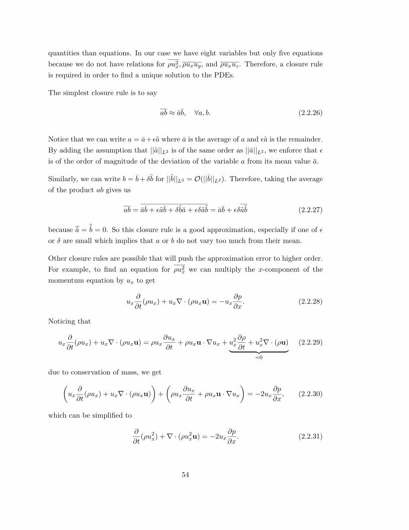
quantities than equations. In our case we have eight variables but only five equations
because we do not have relations for ρu2x, ρuxuy, and ρuxuz. Therefore, a closure rule
is required in order to find a unique solution to the PDEs.
The simplest closure rule is to say
ab ≈ ab, ∀a, b. (2.2.26)
Notice that we can write a = a+εa where a is the average of a and εa is the remainder.
By adding the assumption that ||a||L2 is of the same order as ||a||L2 , we enforce that ε
is of the order of magnitude of the deviation of the variable a from its mean value a.
Similarly, we can write b = b+ δb for ||b||L2 = O(||b||L2). Therefore, taking the average
of the product ab gives us
ab = ab+ εab+ δba+ εδab = ab+ εδab (2.2.27)
because a = b = 0. So this closure rule is a good approximation, especially if one of ε
or δ are small which implies that a or b do not vary too much from their mean.
Other closure rules are possible that will push the approximation error to higher order.
For example, to find an equation for ρu2x we can multiply the x-component of the
momentum equation by ux to get
ux∂
∂t(ρux) + ux∇ · (ρuxu) = −ux
∂p
∂x. (2.2.28)
Noticing that
ux∂
∂t(ρux) + ux∇ · (ρuxu) = ρux
∂ux∂t
+ ρuxu · ∇ux + u2x
∂ρ
∂t+ u2
x∇ · (ρu)︸ ︷︷ ︸
=0
(2.2.29)
due to conservation of mass, we get
(ux
∂
∂t(ρux) + ux∇ · (ρuxu)
)+
(ρux
∂ux∂t
+ ρuxu · ∇ux)
= −2ux∂p
∂x, (2.2.30)
which can be simplified to
∂
∂t(ρu2
x) +∇ · (ρu2xu) = −2ux
∂p
∂x. (2.2.31)
54

Therefore, we can average this to get
∂
∂t(Aρu2
x) +∂
∂x(Aρu3
x) = −2A
(ux∂p
∂x
). (2.2.32)
This means we have an evolution equation for the ρu2x and now only require a closure
rule for higher order terms, for example,
ρu3x =
ρuxρu2x
ρ(2.2.33)
which should give a more accurate approximation than Eq. 2.2.26.
However, the system is more complex because we have another PDE that needs solving,
and we would have to include a closure rule for ux∂p∂x as well. Therefore, we will close
our system by using Eq. 2.2.26 because we are aiming to find a mathematically simple
system that captures the main surge dynamics.
This means that Eqs. 2.2.24 becomes
∂
∂t(Aρuy) +
∂
∂x(Aρuxuy) = 0. (2.2.34)
Since we expect the momentum to change down the length of the pipe, we need to
allow ρux to vary with x. Therefore, the only way to satisfy this equation is to assume
uy = 0. The same argument applied to Eq. 2.2.25 leads to uz = 0.
Therefore, the conservation of mass, momentum and energy for our system becomes
∂
∂t(Aρ) +
∂
∂x(Aρu) = 0, (2.2.35)
∂
∂t(Aρu) +
∂
∂x(Aρu2) = − ∂
∂x(Ap), (2.2.36)
p = κργ , (2.2.37)
where we have used u ≡ ux and dropped the bars for notational ease.
Using Eq. 2.2.37 and the definition of mass flow rate m = Aρu, we can re-write this
55
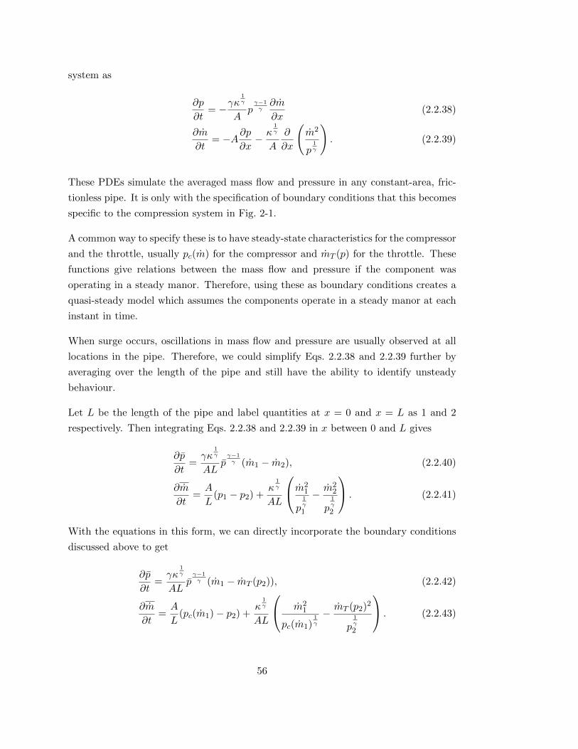
system as
∂p
∂t= −γκ
1γ
Apγ−1γ∂m
∂x(2.2.38)
∂m
∂t= −A∂p
∂x− κ
1γ
A
∂
∂x
(m2
p1γ
). (2.2.39)
These PDEs simulate the averaged mass flow and pressure in any constant-area, fric-
tionless pipe. It is only with the specification of boundary conditions that this becomes
specific to the compression system in Fig. 2-1.
A common way to specify these is to have steady-state characteristics for the compressor
and the throttle, usually pc(m) for the compressor and mT (p) for the throttle. These
functions give relations between the mass flow and pressure if the component was
operating in a steady manor. Therefore, using these as boundary conditions creates a
quasi-steady model which assumes the components operate in a steady manor at each
instant in time.
When surge occurs, oscillations in mass flow and pressure are usually observed at all
locations in the pipe. Therefore, we could simplify Eqs. 2.2.38 and 2.2.39 further by
averaging over the length of the pipe and still have the ability to identify unsteady
behaviour.
Let L be the length of the pipe and label quantities at x = 0 and x = L as 1 and 2
respectively. Then integrating Eqs. 2.2.38 and 2.2.39 in x between 0 and L gives
∂p
∂t=γκ
1γ
ALpγ−1γ (m1 − m2), (2.2.40)
∂m
∂t=A
L(p1 − p2) +
κ1γ
AL
m
21
p1γ
1
− m22
p1γ
2
. (2.2.41)
With the equations in this form, we can directly incorporate the boundary conditions
discussed above to get
∂p
∂t=γκ
1γ
ALpγ−1γ (m1 − mT (p2)), (2.2.42)
∂m
∂t=A
L(pc(m1)− p2) +
κ1γ
AL
m2
1
pc(m1)1γ
− mT (p2)2
p1γ
2
. (2.2.43)
56
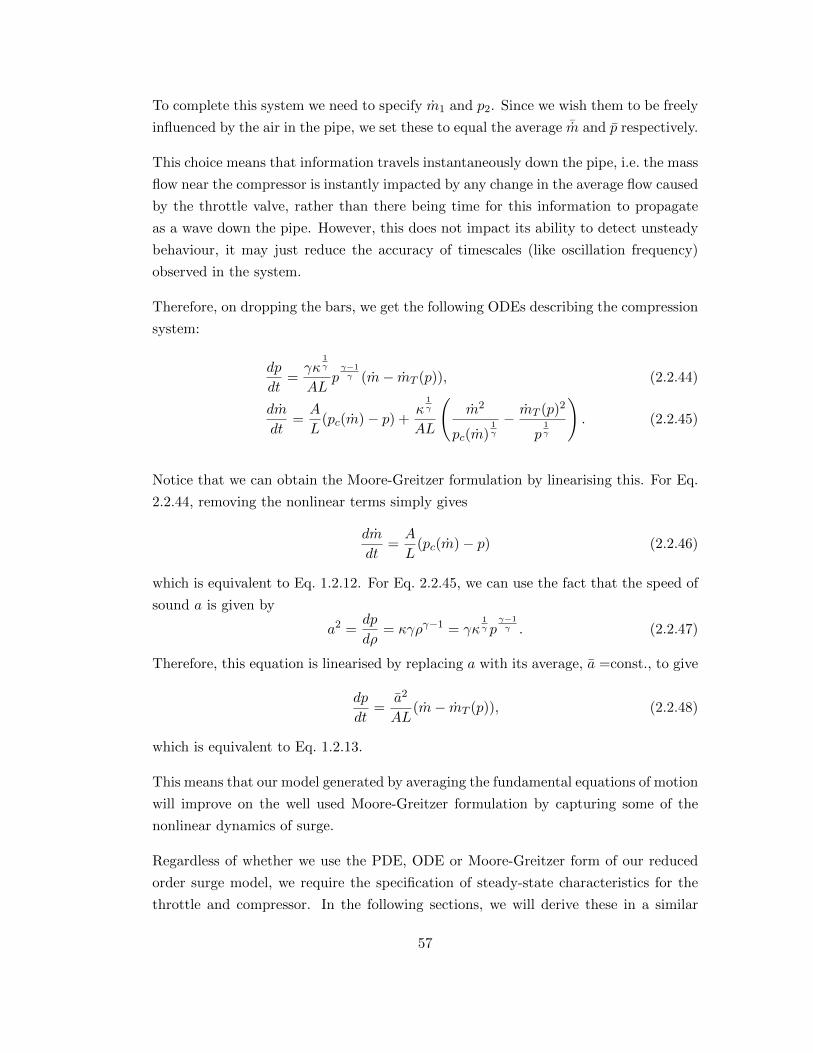
To complete this system we need to specify m1 and p2. Since we wish them to be freely
influenced by the air in the pipe, we set these to equal the average ¯m and p respectively.
This choice means that information travels instantaneously down the pipe, i.e. the mass
flow near the compressor is instantly impacted by any change in the average flow caused
by the throttle valve, rather than there being time for this information to propagate
as a wave down the pipe. However, this does not impact its ability to detect unsteady
behaviour, it may just reduce the accuracy of timescales (like oscillation frequency)
observed in the system.
Therefore, on dropping the bars, we get the following ODEs describing the compression
system:
dp
dt=γκ
1γ
ALpγ−1γ (m− mT (p)), (2.2.44)
dm
dt=A
L(pc(m)− p) +
κ1γ
AL
(m2
pc(m)1γ
− mT (p)2
p1γ
). (2.2.45)
Notice that we can obtain the Moore-Greitzer formulation by linearising this. For Eq.
2.2.44, removing the nonlinear terms simply gives
dm
dt=A
L(pc(m)− p) (2.2.46)
which is equivalent to Eq. 1.2.12. For Eq. 2.2.45, we can use the fact that the speed of
sound a is given by
a2 =dp
dρ= κγργ−1 = γκ
1γ p
γ−1γ . (2.2.47)
Therefore, this equation is linearised by replacing a with its average, a =const., to give
dp
dt=
a2
AL(m− mT (p)), (2.2.48)
which is equivalent to Eq. 1.2.13.
This means that our model generated by averaging the fundamental equations of motion
will improve on the well used Moore-Greitzer formulation by capturing some of the
nonlinear dynamics of surge.
Regardless of whether we use the PDE, ODE or Moore-Greitzer form of our reduced
order surge model, we require the specification of steady-state characteristics for the
throttle and compressor. In the following sections, we will derive these in a similar
57
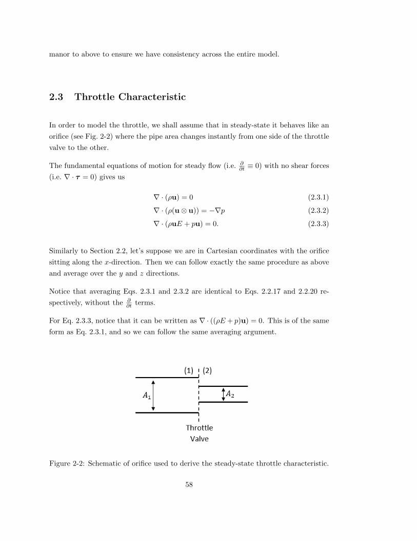
manor to above to ensure we have consistency across the entire model.
2.3 Throttle Characteristic
In order to model the throttle, we shall assume that in steady-state it behaves like an
orifice (see Fig. 2-2) where the pipe area changes instantly from one side of the throttle
valve to the other.
The fundamental equations of motion for steady flow (i.e. ∂∂t ≡ 0) with no shear forces
(i.e. ∇ · τ = 0) gives us
∇ · (ρu) = 0 (2.3.1)
∇ · (ρ(u⊗ u)) = −∇p (2.3.2)
∇ · (ρuE + pu) = 0. (2.3.3)
Similarly to Section 2.2, let’s suppose we are in Cartesian coordinates with the orifice
sitting along the x-direction. Then we can follow exactly the same procedure as above
and average over the y and z directions.
Notice that averaging Eqs. 2.3.1 and 2.3.2 are identical to Eqs. 2.2.17 and 2.2.20 re-
spectively, without the ∂∂t terms.
For Eq. 2.3.3, notice that it can be written as ∇ · ((ρE + p)u) = 0. This is of the same
form as Eq. 2.3.1, and so we can follow the same averaging argument.
Figure 2-2: Schematic of orifice used to derive the steady-state throttle characteristic.
58
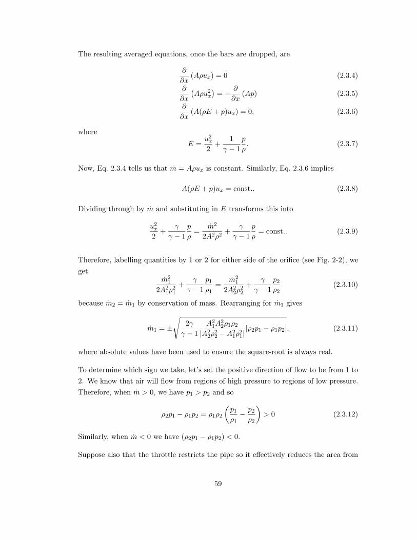
The resulting averaged equations, once the bars are dropped, are
∂
∂x(Aρux) = 0 (2.3.4)
∂
∂x
(Aρu2
x
)= − ∂
∂x(Ap) (2.3.5)
∂
∂x(A(ρE + p)ux) = 0, (2.3.6)
where
E =u2x
2+
1
γ − 1
p
ρ. (2.3.7)
Now, Eq. 2.3.4 tells us that m = Aρux is constant. Similarly, Eq. 2.3.6 implies
A(ρE + p)ux = const.. (2.3.8)
Dividing through by m and substituting in E transforms this into
u2x
2+
γ
γ − 1
p
ρ=
m2
2A2ρ2+
γ
γ − 1
p
ρ= const.. (2.3.9)
Therefore, labelling quantities by 1 or 2 for either side of the orifice (see Fig. 2-2), we
getm2
1
2A21ρ
21
+γ
γ − 1
p1
ρ1=
m21
2A22ρ
22
+γ
γ − 1
p2
ρ2(2.3.10)
because m2 = m1 by conservation of mass. Rearranging for m1 gives
m1 = ±√
2γ
γ − 1
A21A
22ρ1ρ2
|A22ρ
22 −A2
1ρ21||ρ2p1 − ρ1p2|, (2.3.11)
where absolute values have been used to ensure the square-root is always real.
To determine which sign we take, let’s set the positive direction of flow to be from 1 to
2. We know that air will flow from regions of high pressure to regions of low pressure.
Therefore, when m > 0, we have p1 > p2 and so
ρ2p1 − ρ1p2 = ρ1ρ2
(p1
ρ1− p2
ρ2
)> 0 (2.3.12)
Similarly, when m < 0 we have (ρ2p1 − ρ1p2) < 0.
Suppose also that the throttle restricts the pipe so it effectively reduces the area from
59

Figure 2-3: (a) Steady-state throttle characteristic to be used in reduced order surgemodel. The intercept occurs when the flow in the pipe has identical conditions to thaton the other side of the throttle valve (in this case ambient). (b) Incompressible versionof throttle characteristic commonly used in literature.
A to µA, for some fraction µ, and the air after going through the throttle is at ambient
conditions.
Then, the throttle characteristic is given by
mT = sgn(pρamb − pambρ)
√2γ
γ − 1
µ2A2ρρamb|µ2ρ2
amb − ρ2| |pρamb − pambρ|. (2.3.13)
As we saw in Section 2.2, the fact that we have no stress terms means the isentropic
relation holds (see Eq. 2.2.11). Hence, we can simply use that ρ =( pκ
) 1γ , to make this
a function only of p. Figure 2-3(a) shows the resulting characteristic in the mass flow
- pressure plane.
Our formula for the throttle characteristic is slightly different to those typically used
in literature because the orifice equation is usually derived from the incompressible
form of conservation of energy. We decided to derive the compressible form of the
orifice equation to ensure consistency across the model, i.e. the model for the pipes,
compressor and throttle will all assume compressible flow.
As we can see from Fig. 2-3(b), the compressible throttle characteristic is different
from the incompressible version because it has a horizontal asymptote at zero pressure,
which makes sense because pressure is always positive and only zero if a vacuum is
achieved. However, since this mainly affects the case where air is flowing backwards
through the orifice, we could use the incompressible version in studies where the air is
always travelling in a forward direction through the throttle.
60
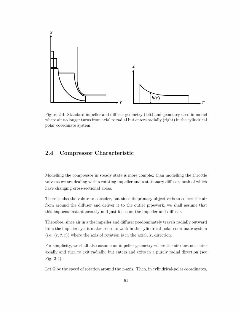
Figure 2-4: Standard impeller and diffuser geometry (left) and geometry used in modelwhere air no longer turns from axial to radial but enters radially (right) in the cylindricalpolar coordinate system.
2.4 Compressor Characteristic
Modelling the compressor in steady state is more complex than modelling the throttle
valve as we are dealing with a rotating impeller and a stationary diffuser, both of which
have changing cross-sectional areas.
There is also the volute to consider, but since its primary objective is to collect the air
from around the diffuser and deliver it to the outlet pipework, we shall assume that
this happens instantaneously and just focus on the impeller and diffuser.
Therefore, since air in a the impeller and diffuser predominately travels radially outward
from the impeller eye, it makes sense to work in the cylindrical-polar coordinate system
(i.e. (r, θ, x)) where the axis of rotation is in the axial, x, direction.
For simplicity, we shall also assume an impeller geometry where the air does not enter
axially and turn to exit radially, but enters and exits in a purely radial direction (see
Fig. 2-4).
Let Ω be the speed of rotation around the x-axis. Then, in cylindrical-polar coordinates,
61
the steady-state component form of the fundamental fluid equations are:
1
r
∂
∂r(rρur) +
1
r
∂
∂θ(ρuθ) +
∂
∂x(ρux) = 0 (2.4.1)
1r∂∂r (rρu2
r) + 1r∂∂θ (ρuruθ) + ∂
∂x(ρurux)− ρu2θr − 2ρΩuθ − ρΩ2r = −∂p
∂r + [∇ · τ ]r (2.4.2)
1
r
∂
∂r(rρuruθ) +
1
r
∂
∂θ(ρu2
θ) +∂
∂x(ρuθux) +
ρuruθr
+ 2ρΩur = −1
r
∂p
∂θ+ [∇ · τ ]θ (2.4.3)
1
r
∂
∂r(rρuxur) +
1
r
∂
∂θ(ρuθux) +
∂
∂x(ρu2
x) = −∂p∂x
+ [∇ · τ ]x (2.4.4)
1
r
∂
∂r(rur(ρE + p)) +
1
r
∂
∂θ(uθ(ρE + p)) +
∂
∂x(ux(ρE + p)) = 0 (2.4.5)
where
E =|u|2
2+
1
γ − 1
p
ρ− Ω2r2
2. (2.4.6)
2.4.1 Isentropic Formulation
Similarly to the previous two sections, we begin by simplifying the system by assuming
there are no shear stress forces, i.e. ∇ · τ = 0. This means that we have isentropic flow
and the relation p = κργ holds. This can be proven by a similar argument to that of
Eq. 2.2.6 - 2.2.11 with the rotational terms included.
Now, since the impeller and diffuser are distinct components in the centrifugal com-
pressor, we will consider them separately in the model formulation.
Impeller
Let us assume we have straight radial blades, so uθ = 0 in the impeller channels. This
results in:
1
r
∂
∂r(rρur) +
∂
∂x(ρux) = 0 (2.4.7)
1
r
∂
∂r(rρu2
r) +∂
∂x(ρurux)− ρΩ2r = −∂p
∂r(2.4.8)
62
2ρΩur = −1
r
∂p
∂θ(2.4.9)
1
r
∂
∂r(rρuxur) +
∂
∂x(ρu2
x) = −∂p∂x
(2.4.10)
1
r
∂
∂r(rur(ρE + p)) +
∂
∂x(ux(ρE + p)) = 0. (2.4.11)
Notice that this has removed all mention of θ apart from in the second momentum
equation (Eq. 2.4.9). This equation specifies that there will be a pressure gradient in
the tangential direction due to the Coriolis force. We can therefore make the simplifying
assumption that all variables (except p) are constant with θ and can be considered as
a function of r and x only.
Using this, we can integrate Eq. 2.4.9 to get
p(r, θ, x) = −2Ωrρur(r, x)θ + p(r, x) (2.4.12)
where p is the constant of integration chosen so that it corresponds to the pressure in
the centre of a channel. This means the channel walls are at
(π + 2πk)
nb, k = 0, .., nb − 1 (2.4.13)
where nb is the number of blades. Therefore, assuming each impeller channel behaves
identically, we can take the average of this over the θ direction by
p(r, x) =1
2π
nb∑
i=1
∫ πnb
− πnb
p(r, θ, x) dθ. (2.4.14)
This results in p = p(r, x) because
−Ωrρur(r, x)
π
nb∑
i=1
∫ πnb
− πnb
θ dθ = 0. (2.4.15)
Therefore, by approximating p(r, θ, x) by its value at the centre of the impeller channel,
we no longer need Eq. 2.4.9 and we have a system that is only dependent on r and x.
Since we want to understand the dynamics as we travel through the compressor, it
makes sense to average the flow over the x-direction so we end up with a 1D model for
flow in the radial direction.
63
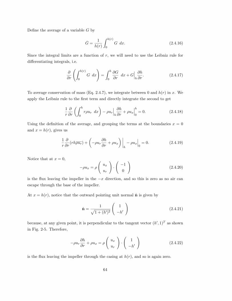
Define the average of a variable G by
G =1
h(r)
∫ h(r)
0G dx. (2.4.16)
Since the integral limits are a function of r, we will need to use the Leibniz rule for
differentiating integrals, i.e.
∂
∂r
(∫ h(r)
0G dx
)=
∫ h
0
∂G
∂rdx+G
∣∣∣h
∂h
∂r. (2.4.17)
To average conservation of mass (Eq. 2.4.7), we integrate between 0 and h(r) in x. We
apply the Leibniz rule to the first term and directly integrate the second to get
1
r
∂
∂r
(∫ h
0rρur dx
)− ρur
∣∣∣h
∂h
∂r+ ρux
∣∣∣h
0= 0. (2.4.18)
Using the definition of the average, and grouping the terms at the boundaries x = 0
and x = h(r), gives us
1
r
∂
∂r(rhρur) +
(−ρur
∂h
∂r+ ρux
) ∣∣∣∣h
− ρux∣∣∣0
= 0. (2.4.19)
Notice that at x = 0,
−ρux = ρ
(ux
ur
)·(−1
0
)(2.4.20)
is the flux leaving the impeller in the −x direction, and so this is zero as no air can
escape through the base of the impeller.
At x = h(r), notice that the outward pointing unit normal n is given by
n =1√
1 + (h′)2
(1
−h′
)(2.4.21)
because, at any given point, it is perpendicular to the tangent vector (h′, 1)T as shown
in Fig. 2-5. Therefore,
−ρur∂h
∂r+ ρux = ρ
(ux
ur
)·(
1
−h′
)(2.4.22)
is the flux leaving the impeller through the casing at h(r), and so is again zero.
64
Figure 2-5: Height of impeller blade given by the function x = h(r). The outwardpointing unit normal, n, at any point r∗ is perpendicular to the tangent at that point.
This means that the average of Eq. 2.4.7 is
1
r
∂
∂r(rhρur) = 0. (2.4.23)
Following exactly the same approach for Eqs. 2.4.8, 2.4.10, and 2.4.11, gives
1
r
∂
∂r(rhρu2
r)− hρΩ2r = − ∂
∂r(hp) + p
∣∣∣h
∂h
∂r, (2.4.24)
1
r
∂
∂r(rhρurux) = −p
∣∣∣h
0, (2.4.25)
1
r
∂
∂r(rhρurE + rhurp) = 0. (2.4.26)
Similarly to the approach in Section 2.2, we assume that ab = ab,∀a, b.
We will also assume that the pressure is constant in the x direction, so
p∣∣∣h
= p∣∣∣0
= p. (2.4.27)
This means that Eq. 2.4.25 reduces to
1
r
∂
∂r(rhρurux) = 0, (2.4.28)
and so we need to assume ux = 0 so no restrictions are placed on how ρur varies with
r through this equation.
65
Thus, on dropping bars, the averaged equations of motion for steady flow through the
impeller are
1
r
∂
∂r(rhρur) = 0 (2.4.29)
1
r
∂
∂r(rhρu2
r)− hρΩ2r = −h∂p∂r
(2.4.30)
1
r
∂
∂r
(rhρur
(u2r
2+
γ
γ − 1
p
ρ− Ω2r2
2
))= 0 (2.4.31)
where
E =u2r
2+
1
γ − 1
p
ρ− Ω2r2
2. (2.4.32)
In order to simplify this system, we can replace the energy equation (Eq. 2.4.31) with
the isentropic condition p = κργ , and integrate Eq. 2.4.29 to give
q = rhρur, (2.4.33)
where q is a constant. Notice also that q = m2π because the cross sectional area of the
impeller is A = 2πrh.
Therefore, substituting these in Eq. 2.4.30 and dividing through by hρ, gives
q
rhρ
∂ur∂r− Ω2r = −γκργ−2∂ρ
∂r. (2.4.34)
Noticing that qrhρ = ur and integrating results in
u2r
2− Ω2r2
2= − κγ
γ − 1ργ−1 + c1, (2.4.35)
which, when written entirely in terms of ρ, becomes
q2
2r2h2ρ2+
κγ
γ − 1ργ−1 =
Ω2r2
2+ c1, (2.4.36)
for constant of integration c1 that can be found by using the boundary condition that
ρ = ρamb at the impeller inlet.
Equation 2.4.36 can therefore be solved to find the density ρ, and hence p = κργ , at
each mass flow m = 2πq for a chosen impeller speed setting, Ω.
66

Diffuser
In the diffuser, we can assume that the flow is independent of θ as a vaneless diffuser
is axisymmetric. Also, Ω = 0 since the diffuser is not a rotating part. Therefore, the
fundamental equations of motion give us
1
r
∂
∂r(rρur) +
∂
∂x(ρux) = 0 (2.4.37)
1
r
∂
∂r(rρu2
r) +∂
∂x(ρurux)− ρu2
θ
r= −∂p
∂r(2.4.38)
1
r
∂
∂r(rρuruθ) +
∂
∂x(ρuθux) +
ρuruθr
= 0 (2.4.39)
1
r
∂
∂r(rρuxur) +
∂
∂x(ρu2
x) = −∂p∂x
(2.4.40)
1
r
∂
∂r(rur(ρE + p)) +
∂
∂x(ux(ρE + p)) = 0 (2.4.41)
This system is already a function of r and x only. Therefore, as before, we average over
the axial height to get a 1D model for the flow in the radial direction.
In the diffuser, the channel height remains constant, so we can perform averaging
without needing the Leibniz rule. Also, our no-flux boundary conditions simply become
ux∣∣0
= ux∣∣h
= 0. (2.4.42)
Therefore, the five averaged equations of motion are
1
r
∂
∂r(rhρur) = 0, (2.4.43)
1
r
∂
∂r(rhρu2
r)−hρu2
θ
r= −h∂p
∂r, (2.4.44)
1
r
∂
∂r(rhρuruθ) +
hρuruθr
= 0, (2.4.45)
1
r
∂
∂r(rhρurux) = −p
∣∣∣h
0, (2.4.46)
1
r
∂
∂r(rh(ρurE + urp)) = 0, (2.4.47)
respectively.
As with the impeller, we assume that ab = ab and that the pressure, p, is constant in
x. Hence, Eq. 2.4.46 requires us to assume ux = 0 in order to not apply additional
67
restriction on ρur through this equation.
Therefore, on dropping the bars, the equations of motion in the diffuser are
1
r
∂
∂r(rhρur) = 0 (2.4.48)
1
r
∂
∂r(rhρu2
r)−hρu2
θ
r= −h∂p
∂r(2.4.49)
1
r
∂
∂r(rhρuruθ) +
hρuruθr
= 0 (2.4.50)
1
r
∂
∂r
(rhρur
(u2r
2+u2θ
2+
γ
γ − 1
p
ρ
))= 0 (2.4.51)
where
E =u2r
2+u2θ
2+
1
γ − 1
p
ρ. (2.4.52)
To simplify this system, we can again replace the energy equation (Eq. 2.4.51) with the
isentropic relation p = κργ . We can also integrate Eq. 2.4.48 to get q = rhρur, where
q is constant.
Therefore, we can take out q = rhρur from the differential in Eq. 2.4.50 and divide
through by hρur to get∂uθ∂r
+uθr
= 0. (2.4.53)
This can be integrated to give
uθ =c
r(2.4.54)
for a constant c that can be found by using the boundary condition of uθ = Ωr at the
impeller tip, ie. c = Ωr2tip.
Substituting these relations for q, uθ, and p into Eq. 2.4.49 and dividing by hρ results
in
ur∂ur∂r−
Ω2r4tip
r3= −γκργ−2∂ρ
∂r(2.4.55)
because ur = qrhρ . Therefore, integrating this and writing ur in terms of q, gives us
q2
2r2h2ρ2+
κγ
γ − 1ργ−1 = −
Ω2r4tip
2r2+ c2, (2.4.56)
where c2 is a constant of integration that can be found by applying the boundary
condition that density is continuous at the impeller - diffuser interface.
Therefore, this can be solved to find the density, ρ, through the diffuser at each mass
68
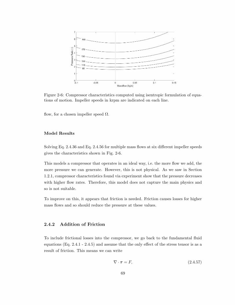
Figure 2-6: Compressor characteristics computed using isentropic formulation of equa-tions of motion. Impeller speeds in krpm are indicated on each line.
flow, for a chosen impeller speed Ω.
Model Results
Solving Eq. 2.4.36 and Eq. 2.4.56 for multiple mass flows at six different impeller speeds
gives the characteristics shown in Fig. 2-6.
This models a compressor that operates in an ideal way, i.e. the more flow we add, the
more pressure we can generate. However, this is not physical. As we saw in Section
1.2.1, compressor characteristics found via experiment show that the pressure decreases
with higher flow rates. Therefore, this model does not capture the main physics and
so is not suitable.
To improve on this, it appears that friction is needed. Friction causes losses for higher
mass flows and so should reduce the pressure at these values.
2.4.2 Addition of Friction
To include frictional losses into the compressor, we go back to the fundamental fluid
equations (Eq. 2.4.1 - 2.4.5) and assume that the only effect of the stress tensor is as a
result of friction. This means we can write
∇ · τ = F, (2.4.57)
69

where F is a friction function. Notice that this is friction per unit volume because,
during derivation of the fundamental fluid equations, all terms were divided by volume.
We will assume that F relates to skin fiction, rather than the internal friction of the
fluid. This is defined as the shearing stress exerted by the fluid on the surface over
which it flows [56]. Therefore,
F = −τwS (2.4.58)
where τw is the wall shearing stress, and S is the surface area (per unit volume). This
can be written as
F = −1
2fρu|u|S (2.4.59)
where f is the fanning friction factor [57]. Notice that u|u| ensures that the friction
always acts against the flow.
For ease of solving the system ODEs, we will simplify this further to
F = −1
2fρu|ur|S (2.4.60)
and assume that the friction factor f encompasses the difference, i.e.
f ∝
√u2r + u2
θ
ur. (2.4.61)
In the impeller this f is equivalent to the fanning friction factor as uθ = 0, however
it will be slightly different in the diffuser. In practice, we will fit the friction factor to
experimental data in order to find an accurate value for simulations.
To generate a model for the steady state operation of the compressor we can follow
exactly the same procedure as in Section 2.4.1 with the addition of F in the momentum
equations to give
1
r
∂
∂r(rhρur) = 0 (2.4.62)
1
r
∂
∂r(rhρu2
r)− hρΩ2r = −h∂p∂r
+ hFr (2.4.63)
1
r
∂
∂r
(rhρur
(u2r
2+
γ
γ − 1
p
ρ− Ω2r2
2
))= 0 (2.4.64)
70

for the impeller and
1
r
∂
∂r(rhρur) = 0, (2.4.65)
1
r
∂
∂r(rhρu2
r)−hρu2
θ
r= −h∂p
∂r+ hFr, (2.4.66)
1
r
∂
∂r(rhρuruθ) +
hρuruθr
= hFθ, (2.4.67)
1
r
∂
∂r
(rhρur
(u2r
2+u2θ
2+
γ
γ − 1
p
ρ
))= 0, (2.4.68)
for the diffuser, where the bars have been dropped for ease.
To simplify these systems of ODEs, note that we no longer satisfy the isentropic relation
because of the additional frictional losses. Therefore, for the impeller, we integrate Eqs.
2.4.62 and 2.4.64 to get q = rhρur and
u2r
2+
γ
γ − 1
p
ρ− Ω2r2
2= EI (2.4.69)
respectively, where q and EI are both constants. Rearranging Eq. 2.4.69 for p and
substituting into Eq. 2.4.63 along with q and
Fr = −1
2fρ|ur|urSI , SI = 2
(nb
2πr+
1
h
), (2.4.70)
for number of impeller blades nb, results in
∂ρ
∂r=−ρq2
(1r + 1
h∂h∂r
)− Ω2r3h2ρ3 + γfρ|q|q
(nb2πr + 1
h
)(γ+1
2
)q2 − (γ − 1)
(Ω2r2
2 + EI
)r2h2ρ2
, (2.4.71)
which is an ODE that can be solved quickly via numerical methods, like Runga-Kutta,
for the density ρ.
Similarly, for the diffuser, we integrate Eqs. 2.4.65 and 2.4.68 to get q = rhρur and
u2r
2+u2θ
2+
γ
γ − 1
p
ρ= ED, (2.4.72)
and substitute these along with
Fr = −1
2fρ|ur|urSD, SD =
2
h, (2.4.73)
71

into Eq. 2.4.66 to get
∂ρ
∂r=−ρq2
r − r2h2ρ3(γu2θr + (γ − 1)uθ
∂uθ∂r
)+ γ fhρ|q|q(
γ+12
)q2 + (γ − 1)
(u2θ2 − ED
)r2h2ρ2
. (2.4.74)
Finally, Eq. 2.4.67 is given by
1
r
∂
∂r(rhρuruθ) +
hρuruθr
= −h1
2fρ|ur|uθSD (2.4.75)
because the friction Fθ opposes the momentum of the fluid. Therefore, taking q = rhρur
out of the derivative and dividing by hρur gives us
∂uθ∂r
+uθr
= −f2
sgn(ur)uθSD. (2.4.76)
Using the fact that SD = 2h and integrating results in
uθ =c
re−sgn(ur)( fh)r (2.4.77)
where sgn(ur) = ±1 depending on the sign of ur, and c is the constant of integration.
Since ur and uθ have the same sign, we could also write this as
uθ =c
re−sgn(uθ)( fh)r. (2.4.78)
Finally, we know that
c = Ωr2tipe
( fh)rtip (2.4.79)
because the tangential velocity is assumed to be continuous at the impeller - diffuser
interface (i.e. uθ = Ωr at r = rtip).
This means that Eq. 2.4.74 is an ODE purely for density ρ and can be solved numerically
in the same manor as Eq. 2.4.71.
Model Results
Solving Eqs. 2.4.71 and 2.4.74 for multiple mass flows at six different impeller speeds
results in the compressor characteristics shown in Fig. 2-7.
72

Figure 2-7: Compressor characteristics map computed by averaging the fundamentalfluid equations with the inclusion of skin friction. Impeller speeds in krpm are indicatedon each line.
This model is now able to capture a cubic-like shape similar to that seen in experiments
(see Section 1.2.1). This means that friction plays a vital role in the operation of a
compressor, and so cannot be left out of any model.
However, this model still is missing some important dynamics. Using this characteristic
in the reduced order surge model developed in Section 2.2 (both the nonlinear ODEs
and the Moore-Greitzer version) we only ever see stable behaviour. Figure 2-8 shows
this at a low mass flow value where we would expect to see surge.
In Section 1.2.1, we saw that the characteristics observed experimentally had a local
minimum at zero mass flow, rather than the point of inflection we have obtained. This
Figure 2-8: Stable operation using the Moore-Greitzer model. Left: Trajectory ofcompressor operation in mass flow-pressure plane. Right: Pressure and mass flowtraces of compressor operation with time.
73

Figure 2-9: Determination of shape of compressor characteristics by looking at differentlosses [1]. The characteristic (A-D) is created by subtracting the loss curves shown atthe bottom of the graph.
suggests that the reason our characteristic behaves stably is that it is monotonically
decreasing.
Therefore, to achieve a compressor characteristic that exhibits surge behaviour, we
need to include some losses that occur for small mass flow rates. According to Watson
and Janota [1], the pressure drop observed at low mass flow rates are due to incidence
losses (see Fig. 2-9).
2.4.3 Addition of Incidence Loss
Incidence losses occur when the flow entering the impeller does not perfectly match the
blades. Figure 2-10 shows that flow entering the impeller channel at an angle larger
than the blade angle can cause the flow to separate. This separation can be modelled
as a blockage in the channel.
To represent this blockage we create a stall function, ξ, where m = ξAρur. This means
that ξA represents the area of the channel that is available for the flow to pass through.
Suppose β is the angle of the flow entering the impeller and βB is the impeller inlet
blade angle. Then for β ≤ βB, we assume there are no incidence losses and so ξ = 1.
For β > βB, we can find the stall function by considering the velocity as a function of
the mass flow, i.e. ur(m) = mξAρ .
74

Figure 2-10: Left: Flow matches the blades perfectly, so zero incidence loss. Right:Flow enters the impeller channel at an angle β > βB, so we have incidence losses. Herethe flow separates and we assume the stalled flow causes a blockage in the channel.
We would like ξ to be a smooth function, therefore we will make the velocity continu-
ously differentiable at β = βB, i.e.
ur(mB) =mB
Aρ, (2.4.80)
durdm
(mB) =1
Aρ. (2.4.81)
Also, at zero mass flow, we would expect the velocity to be zero. So we have another
condition of
ur(0) = 0. (2.4.82)
We desire a free parameter in the stall function in order to set the strength of this stall
based on experimental data. Therefore, with three conditions and a free parameter,
the simplest function we can use to describe the stalled velocity is a cubic:
ur = am3 + bm2 + cm+ d. (2.4.83)
Differentiating this gives
durdm
= 3am2 + 2bm+ c. (2.4.84)
75
Then, condition 2.4.82 immediately gives us d = 0, and conditions 2.4.80 and 2.4.81
gives us
mB
Aρ= am3
B + bm2B + cmB, (2.4.85)
1
Aρ= 3am2
B + 2bmB + c, (2.4.86)
respectively. Choosing a as our free parameter and solving these for b and c gives us
b = −2amB, (2.4.87)
c =1
Aρ+ am2
B. (2.4.88)
Therefore, our stalled velocity is given by
ur(m) = am3 − 2amBm2 +
(1
Aρ+ am2
B
)m. (2.4.89)
Using the fact that ur = mξAρ and rearranging for ξ results in
ξ(β) =1
1 + a(
1− tanβBtanβ
)2 , (2.4.90)
where a = aAρm2B, because
m
mB=
tanβBtanβ
. (2.4.91)
Note that this doesn’t change any of the ODEs in Section 2.4.2 because it only influences
the definition of the constant q. Previously, q = m2π whereas to incorporate the stalling
we can change this to be
q =m
2πξ(β). (2.4.92)
The resulting compressor characteristic and its behaviour when integrated into the
nonlinear reduced order surge model are presented in the paper included in the following
section.
76

This declaration concerns the article entitled:
Modeling Axisymmetric Centrifugal Compressor Characteristics from First Principles
Publication status (tick one)
Draft manuscript Submitted In review Accepted Published X
Publication details (reference)
Powers, K. H., Brace, C. J., Budd, C. J., Copeland, C. D., and Milewski, P. A. (August 25, 2020). "Modeling Axisymmetric Centrifugal Compressor Characteristics from First Principles."
ASME. J. Turbomach. September 2020; 142(9): 091010. https://doi.org/10.1115/1.4047616
Copyright status (tick the appropriate statement)
I hold the copyright for this material Copyright is retained by the publisher, but I have
been given permission to replicate the material here X
Candidate’s contribution to the paper (provide details, and also indicate as a percentage)
The contribution of Katherine Powers to the paper is as follows:
• Formulation of ideas (80%) with advice from supervisors
• Derivation of equations for the mathematical models (90%)
• Writing MATLAB code and creating of numerical simulations (100%)
• Comparing numerical simulations to given experimental data, and analysing of the results (100%)
• Presentation of data in journal format (100%)
Statement from Candidate
This paper reports on original research I conducted during the period of my Higher Degree by Research candidature.
Signed
Date
26/02/2021
2.5 Paper 1: Modelling Axisymmetric Centrifugal Com-
pressor Characteristics from First Principles
77

Katherine H. PowersDepartment of Mathematical Sciences,
University of Bath,Claverton Down,
Bath BA2 7AY, UKe-mail: [email protected]
Chris J. BraceDepartment of Mechanical Engineering,
University of Bath,Claverton Down,
Bath BA2 7AY, UKe-mail: [email protected]
Chris J. BuddDepartment of Mathematical Sciences,
University of Bath,Claverton Down,
Bath BA2 7AY, UKe-mail: [email protected]
Colin D. CopelandSchool of Sustainable Energy Engineering,
Simon Fraser University,University Drive,
Surrey V3T 0N1, BC, Canadae-mail: [email protected]
Paul A. MilewskiDepartment of Mathematical Sciences,
University of Bath,Claverton Down,
Bath BA2 7AY, UKe-mail: [email protected]
Modeling AxisymmetricCentrifugal CompressorCharacteristics From FirstPrinciplesTurbochargers are a vital component for aiding engine manufacturers in meeting the latestemissions standards. However, their range of operation is limited for low mass flows bycompressor surge. Operation in surge results in pressure and mass flow oscillations thatare often damaging to the compressor and its installation. Since surge is a highlycomplex flow regime, full unsteady three-dimensional models are generally too computa-tionally expensive to run. The majority of current low-dimensional surge models use acubic compressor characteristic that needs to be fitted to experimental data. Therefore,each time a compressor is studied using these models, costly experimental testing isrequired. In this paper, a new technique for obtaining an axisymmetric centrifugal compres-sor characteristic is presented. This characteristic is built using the equations of mass,momentum, and energy from first principles in order to provide a more complete modelthan those currently obtained via experimental data. This approach enables us to explainthe resulting cubic-like shape of the characteristic and hence to identify impeller inletstall as a route into surge. The characteristic is used within a quasi-steady, map-basedsurge model in order to demonstrate its ability to predict the onset of surge while only pro-viding geometric data as input. Validation is provided for this model by a discussion of thequalitative flow dynamics and a good fit to experimental data, especially for low impellerspeeds and pressure ratios. [DOI: 10.1115/1.4047616]
Keywords: centrifugal compressors, compressor stall, surge, modeling
IntroductionThere are a huge number of applications for centrifugal compres-
sors [1]. Although the methodology presented in this paper is appli-cable to all centrifugal compressors (via the extension of models by,for example, Macdougal and Elder [2] who developed a one-dimensional (1D) map-based model for process plant applications),we will focus on the application to turbocharger compressors for theautomotive industry.Turbocharger compressors are normally used to increase the
power output of smaller engines, so they can be used in place oflarger naturally aspirated ones, making the vehicle more environ-mentally friendly [3]. They need a wide stable operating range,but this range is limited by surge at low mass flow rates andchoke at high mass flow rates.Surge is an instability that results in audible mass flow and pres-
sure oscillations that would be off-putting to any driver. Moreover,these oscillations, in combination with an increase in temperature,often damage the compressor or its installation.Surge is commonly found to be triggered by some form of stall.
There are two main types of stall. The first can occur at the inlet tothe impeller or a vaned diffuser and is caused by incidence. Thismeans that, as mass flow decreases, the inlet flow angle increasesand causes a separation of the flow at the blade or vane wall [4].In the impeller, this stall can pass between neighboring channelsto become a rotating stall. The second type is often seen in a
vaneless diffuser and is caused by recirculation. This is where fric-tion reduces the radial velocity of the flow near the shroud-side wallof the diffuser, reducing its spiral angle so that it is swept back intothe impeller [4].The stalling of the impeller and diffuser can occur individually or
simultaneously but are not independent as stall in one componentinfluences the behavior of stall in the other. There is extensive liter-ature on the stall and surge behavior of compressors, for example,Refs. [5–9].Since surge limits the amount of boost provided at low engine
speeds, there is a desire to operate close to surge without enteringit for prolonged periods of time. Therefore, it becomes essentialto create models that can predict the location of the surge regionas well as aid understanding of the flow dynamics near that region.A very common numerical modeling approach is computational
fluid dynamics (CFD). In a CFD model, a 3D domain is built inthe computer, and a mesh is inserted into it. This mesh divides thedomain into millions of control volumes, or cells, within which theconservation of mass, momentum, and energy equations can besolved numerically [10]. The accuracy of CFD computations hasincreased dramatically over the past decades due to the rapidgrowth in high-speed computing power. However, CFD can strugglewhen modeling large scale phenomena that depend on small scaleeffects because it is too computationally expensive to perform thisdirect numerical simulation with the required fineness of mesh[10]. Since surge cycles often experience local or small scale phe-nomena like rotating stall, recirculation, and eddies, full unsteady3D CFD is required to completely capture the dynamics. However,the computational cost of this is not suitable for industrial needs [11].Map-based models provide a popular alternative to CFD for mod-
eling surge. All of these models take as an input a compressor map
Contributed by the International Gas Turbine Institute (IGTI) of ASME forpublication in the JOURNAL OF TURBOMACHINERY. Manuscript received October 14,2019; final manuscript received April 7, 2020; published online August 25, 2020.Assoc. Editor: David G. Bogard.
Journal of Turbomachinery SEPTEMBER 2020, Vol. 142 / 091010-1Copyright © 2020 by ASME78

that has been extended beyond the surge point and into reversedflows. The speed lines on these extended compressor maps areoften referred to as compressor characteristics.Usually, these models assume that at any given time, the compres-
sor is operating in steady-state, and so are quasi-steady in nature.There are many examples of these models in the literature forvarious compressor types and applications [6,12–15]. However,there has been some work on unsteady 1D models that incorporatethe compressor map as a boundary condition [16,17].The majority of these models are based on a nonlinear model by
Greitzer [18]. Greitzer modeled an axial compression system by useof two actuator disks, one to represent the compressor and the otherto represent the throttle valve. These are connected together by apipe and a large plenum. The flow is considered incompressiblewithin the pipe and to have negligible kinetic energy within theplenum. This generates a set of ordinary differential equations(ODEs) to model the behavior of flow in the compression system,for example, the Moore-Greitzer model [18,19]
dΦdt
= B(ψc − Ψ) (1)
dΨdt
=1B(Φ − ψ−1
T ) (2)
for nondimensional mass flow,Φ, and pressure, Ψ, where ψc and ψTare compressor and throttle characteristics, respectively.For the throttle characteristic ψT, the Orifice equation [19]:
ψT = ξT0 +1
ξ2TΦ2 (3)
is typically used.There have been three main approaches for obtaining the com-
pressor characteristics. The first is through complex experimentalstudies, for example, Koff and Greitzer [20] proposed a cubic-likeshape after experimentally testing an axial compressor in variousflow regimes. The curve was reasonably straightforward to deter-mine in backflow and steady forward flow regimes. However,when rotating stall appeared, the shape was more difficult to deter-mine, and so transients were analyzed and an argument was madefor having a smoothly varying characteristic based on the behaviorof diffuser stall. This has been done more recently for small centrif-ugal compressors by Galindo et al. [21], also producing a cubic-likecurve.The second approach is via curve fitting and extrapolation. The
most common technique is to use the cubic relation proposed byMoore and Greitzer [22], i.e.
ψc = ψc0 + H 1 +23
ΦW
− 1
( )−12
ΦW
− 1
( )3[ ]
(4)
with parameters H and W found through fitting to experimentalcompressor map data. However, other curve fitting techniqueshave been proposed, including ones involving Chebyshev polyno-mials in order to capture more features of the characteristics [23],and ones involving elliptic equations in order to adjust the charac-teristic for different settings on a variable-geometry diffuser [24].The third is via mean-line modeling. In a mean-line model, the
compressor is divided into sections over which the equations ofmotion and loss models are evaluated. Most of the mean-linemodels follow the meridional path of the compressor and typicallysplit it into sections for the inlet, impeller, diffuser, and volute[25,26]. However, there are two-zone models that have primaryand secondary flow sections within the impeller in order to accountfor slip [27]. Themajority of thesemean-linemodels apply empiricalloss models to the sections. Typical collections of loss models forcompressors can be found in Refs. [28–30]. These loss modelsusually have loss coefficients that need to be tuned to the particularcompressor that is being studied, which makes mean-line modelingstill partially reliant on data or CFD simulation.
The advantage of the purely experimental approach for findingcompressor characteristics is its simplicity because reading dataor evaluating polynomial-like expressions is very quick computa-tionally. However, map-based surge models are sensitive to theshape of the compressor characteristic, so it is vital to understandthis fully, and an experimental approach does not give us anyinsight into the reason why we get this shape of the curve. In addi-tion, since surge is a system phenomenon, experimentally measuredsurge can be limited to the particular experimental setup and not, aswould be desirable, any compressor installation.The mean-line model approach can provide some understanding
of the characteristic’s shape because it is based in part on the phys-ical equations of motion, and a tuned mean-line model producessome good results. However, this model usually still requires com-pressor specific data to tune the loss coefficients. Ideally, we wouldlike a model that works for every type of compressor using onlyknown information, like geometry; therefore, any parameters inthe model need to be universal.In this paper, compressor characteristics are generated through
simulations of a physical model for the compressor. This physicalmodel is derived from first principles and uses inputs solely fromgeometry. It has been designed to be as simple as possible whilestill capturing the dynamics of surge. Therefore, it contains aminimal number of parameters and has found relations for thesethat make them universally applicable. The strength of having amathematically simple model is that it can be used for things likebifurcation analysis, which is a powerful tool to study the dynamicsof surge as parameters, such as geometrical dimensions, are changed.Since the model has been built from physical principles and is
theoretical in nature, it gives us a new understanding of the stalland surge phenomena, which in turn will help in the design offuture compressors. To the authors’ knowledge, this is the firsttime that such a model has been created, and it makes an importantstep in updating the low-dimensional surge models that haveremained relatively unchanged over the past 30 years. This novelapproach will enable low-dimensional surge models to be a usefultool for turbocharger designers, as it will provide insight into thesurge limitations of a new design while reducing the need fortesting during preliminary design stages.
Equations of MotionThe key physical laws needed for deriving a model for a com-
pressor from first principles are conservation of mass
∂ρ∂t
+ ∇ · (ρu) = 0 (5)
conservation of momentum in a rotating frame
∂∂t(ρu) + ∇ · (ρ(u⊗ u)) + 2ρ(Ω × u) + ρ(Ω × (Ω × r)) = ρg
−∇p + ∇ · τ (6)
and conservation of energy
∂∂t(ρE) + ∇ · (ρuE + pu) − ∇ · (τ · u) = ρQ (7)
In the inertial frame of reference,
E =|u|22
+ U (8)
where U is the specific internal energy. However, when we are in arotating frame of reference, E becomes the relative specific energy,so
E +Ω2r2
2=|u|22
+ U (9)
to take into account the energy added to the flow by the rotation.
091010-2 / Vol. 142, SEPTEMBER 2020 Transactions of the ASME79
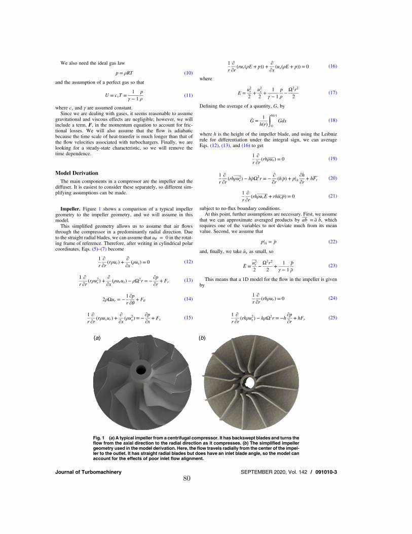
We also need the ideal gas law
p = ρRT (10)
and the assumption of a perfect gas so that
U = cvT =1
γ − 1p
ρ(11)
where cv and γ are assumed constant.Since we are dealing with gases, it seems reasonable to assume
gravitational and viscous effects are negligible; however, we willinclude a term, F, in the momentum equation to account for fric-tional losses. We will also assume that the flow is adiabaticbecause the time scale of heat-transfer is much longer than that ofthe flow velocities associated with turbochargers. Finally, we arelooking for a steady-state characteristic, so we will remove thetime dependence.
Model DerivationThe main components in a compressor are the impeller and the
diffuser. It is easiest to consider these separately, so different sim-plifying assumptions can be made.
Impeller. Figure 1 shows a comparison of a typical impellergeometry to the impeller geometry, and we will assume in thismodel.This simplified geometry allows us to assume that air flows
through the compressor in a predominantly radial direction. Dueto the straight radial blades, we can assume that uθ = 0 in the rotat-ing frame of reference. Therefore, after writing in cylindrical polarcoordinates, Eqs. (5)–(7) become
1r
∂∂r
(rρur) +∂∂x
(ρux) = 0 (12)
1r
∂∂r
(rρu2r ) +∂∂x
(ρurux) − ρΩ2r = −∂p∂r
+ Fr (13)
2ρΩur = −1r
∂p∂θ
+ Fθ (14)
1r
∂∂r
(rρuxur) +∂∂x
(ρu2x ) = −∂p∂x
+ Fx (15)
1r
∂∂r
(rur(ρE + p)) +∂∂x
(ux(ρE + p)) = 0 (16)
where
E =u2r2+u2x2+
1γ − 1
p
ρ−Ω2r2
2(17)
Defining the average of a quantity, G, by
G =1
h(r)
∫h(r)0
Gdx (18)
where h is the height of the impeller blade, and using the Leibnizrule for differentiation under the integral sign, we can averageEqs. (12), (13), and (16) to get
1r
∂∂r
(rhρur) = 0 (19)
1r
∂∂r
(rhρu2r ) − hρΩ2r = −∂∂r
(hp) + p|h∂h∂r
+ hFr (20)
1r
∂∂r
(rhρurE + rhurp) = 0 (21)
subject to no-flux boundary conditions.At this point, further assumptions are necessary. First, we assume
that we can approximate averaged products by ab = a b, whichrequires one of the variables to not deviate much from its meanvalue. Second, we assume that
p|h = p (22)
and, finally, we take ux as small, so
E =u2r2−Ω2r2
2+
1γ − 1
p
ρ(23)
This means that a 1D model for the flow in the impeller is givenby
1r
∂∂r
(rhρur) = 0 (24)
1r
∂∂r
(rhρu2r ) − hρΩ2r = −h∂p∂r
+ hFr (25)
Fig. 1 (a) A typical impeller from a centrifugal compressor. It has backswept blades and turns theflow from the axial direction to the radial direction as it compresses. (b) The simplified impellergeometry used in the model derivation. Here, the flow travels radially from the center of the impel-ler to the outlet. It has straight radial blades but does have an inlet blade angle, so the model canaccount for the effects of poor inlet flow alignment.
Journal of Turbomachinery SEPTEMBER 2020, Vol. 142 / 091010-380

1r
∂∂r
rhρuru2r2+
γ
γ − 1p
ρ−Ω2r2
2
( )( )= 0 (26)
where the bars have been dropped for convenience.
Diffuser. The diffuser is non-rotating, so Ω= 0, and we return tothe inertial frame of reference. It is also assumed that the compres-sor has a vaneless diffuser, which allows the assumption that all var-iables are independent of θ.Therefore, in this case, Eqs. (5)–(7) become
1r
∂∂r
(rρur) +∂∂x
(ρux) = 0 (27)
1r
∂∂r
(rρu2r ) +∂∂x
(ρurux) −ρu2θr
= −∂p∂r
+ Fr (28)
1r
∂∂r
(rρuruθ) +∂∂x
(ρuθux) +ρuruθr
= Fθ (29)
1r
∂∂r
(rρuxur) +∂∂x
(ρu2x ) = −∂p∂x
+ Fx (30)
1r
∂∂r
(rur(ρE + p)) +∂∂x
(ux(ρE + p)) = 0 (31)
where
E =u2r2+u2x2+
1γ − 1
p
ρ(32)
Averaging Eqs. (27)–(29) and (31) subject to no-flux conditionsas before, gives
1r
∂∂r
(rhρur) = 0 (33)
1r
∂∂r
(rhρu2r ) −hρu2θr
= −h∂p∂r
+ hFr(34)
1r
∂∂r
(rhρuruθ) +hρuruθ
r= hFθ (35)
1r
∂∂r
(rhρurE + rhurp) = 0 (36)
Therefore, using the same assumptions as we did for the impeller,so that ab = a b and
E =u2r2+u2θ2+
1γ − 1
p
ρ(37)
we get the following system of equations for the diffuser (after drop-ping the bars):
1r
∂∂r
(rhρur) = 0 (38)
1r
∂∂r
(rhρu2r ) −hρu2θr
= −h∂p∂r
+ hFr (39)
1r
∂∂r
(rhρuruθ) +hρuruθ
r= hFθ (40)
1r
∂∂r
rhρuru2r2+u2θ2+
γ
γ − 1p
ρ
( )( )= 0 (41)
Friction. Skin friction is the only type of frictional loss that isconsidered in this model. It is defined as the shear stress exertedby the fluid on the surface over which it flows [31]. Therefore, ifτw denotes the wall shear stress
F = −τwS (42)
⇒ F = −12f ρu2r S (43)
where S denotes the total surface area of the contact faces betweenthe walls and the fluid per unit volume, and
f =τw
12ρu2r
(44)
is the Fanning friction factor [32].Therefore, in the impeller, we have
Fr = −12f ρu2r SI (45)
where
SI = 2nb2πr
+1h
( )(46)
and for the diffuser, we have
Fr = −12f ρu2r SD (47)
Fθ = −12f ρuruθSD (48)
where
SD =2h
(49)
Stalling. The mass flow rate is defined as m = A ρur for a cross-sectional area A. In the diffuser, the area is simply A= 2πrh.However, in the impeller, we can get stalling at the inlet. As seenin Fig. 2, low inlet velocities lead to large flow angles, β, whichresult in flow separation. This region of stalled flow effectivelyblocks part of the channel, and so reduces the area of the channelavailable to the unstalled flow.Therefore, defining the impeller area as A= θrh for
θ =
2π
1 + α 1 −tan βBtan β
( )2( ) β > βB
2π otherwise
⎧⎪⎪⎪⎨⎪⎪⎪⎩
(50)
where βB is the inlet blade angle of the impeller, allows us to takeinto account this stalling. The parameter α is used to control thestrength of the stalling, for example, if A0 is the area of the entirechannel, then the maximum blockage results in an area of (1/(1+α))A0.It is not uncommon to use blockage as a way to represent stalled
flow regimes. Day et al. [33] developed a model for rotating stall inan axial compressor. They noted that stall cells had negligible axialvelocity, whereas the unstalled regions had a higher axial velocitythan expected. This led to them including a stall cell blockageparameter in their model to simulate this.
091010-4 / Vol. 142, SEPTEMBER 2020 Transactions of the ASME81
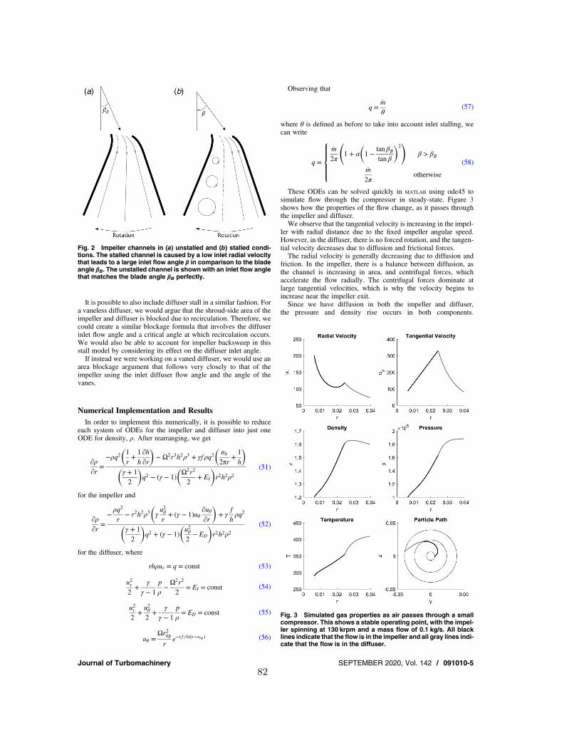
It is possible to also include diffuser stall in a similar fashion. Fora vaneless diffuser, we would argue that the shroud-side area of theimpeller and diffuser is blocked due to recirculation. Therefore, wecould create a similar blockage formula that involves the diffuserinlet flow angle and a critical angle at which recirculation occurs.We would also be able to account for impeller backsweep in thisstall model by considering its effect on the diffuser inlet angle.If instead we were working on a vaned diffuser, we would use an
area blockage argument that follows very closely to that of theimpeller using the inlet diffuser flow angle and the angle of thevanes.
Numerical Implementation and ResultsIn order to implement this numerically, it is possible to reduce
each system of ODEs for the impeller and diffuser into just oneODE for density, ρ. After rearranging, we get
∂ρ∂r
=−ρq2
1r+1h
∂h∂r
( )− Ω2r3h2ρ3 + γf ρq2
nb2πr
+1h
( )γ + 12
( )q2 − (γ − 1)
Ω2r2
2+ EI
( )r2h2ρ2
(51)
for the impeller and
∂ρ∂r
=−ρq2
r− r2h2ρ3 γ
u2θr+ (γ − 1)uθ
∂uθ∂r
( )+ γ
f
hρq2
γ + 12
( )q2 + (γ − 1)
u2θ2− ED
( )r2h2ρ2
(52)
for the diffuser, where
rhρur = q = const (53)
u2r2+
γ
γ − 1p
ρ−Ω2r2
2= EI = const (54)
u2r2+u2θ2+
γ
γ − 1p
ρ= ED = const (55)
uθ =Ωr2tipr
e−( f /h)(r−rtip) (56)
Observing that
q =m
θ(57)
where θ is defined as before to take into account inlet stalling, wecan write
q =
m
2π1 + α 1 −
tan βBtan β
( )2( )
β > βB
m
2πotherwise
⎧⎪⎪⎪⎨⎪⎪⎪⎩
(58)
These ODEs can be solved quickly in MATLAB using ode45 tosimulate flow through the compressor in steady-state. Figure 3shows how the properties of the flow change, as it passes throughthe impeller and diffuser.We observe that the tangential velocity is increasing in the impel-
ler with radial distance due to the fixed impeller angular speed.However, in the diffuser, there is no forced rotation, and the tangen-tial velocity decreases due to diffusion and frictional forces.The radial velocity is generally decreasing due to diffusion and
friction. In the impeller, there is a balance between diffusion, asthe channel is increasing in area, and centrifugal forces, whichaccelerate the flow radially. The centrifugal forces dominate atlarge tangential velocities, which is why the velocity begins toincrease near the impeller exit.Since we have diffusion in both the impeller and diffuser,
the pressure and density rise occurs in both components.
Fig. 3 Simulated gas properties as air passes through a smallcompressor. This shows a stable operating point, with the impel-ler spinning at 130 krpm and a mass flow of 0.1 kg/s. All blacklines indicate that the flow is in the impeller and all gray lines indi-cate that the flow is in the diffuser.
Fig. 2 Impeller channels in (a) unstalled and (b) stalled condi-tions. The stalled channel is caused by a low inlet radial velocitythat leads to a large inlet flow angle β in comparison to the bladeangle βB. The unstalled channel is shown with an inlet flow anglethat matches the blade angle βB perfectly.
Journal of Turbomachinery SEPTEMBER 2020, Vol. 142 / 091010-582

The temperature also rises throughout the compressor because offriction. In the diffuser, friction is acting against both the radialand tangential component of velocity, whereas in the impeller, thetangential velocity is dictated by the impeller rotation and so frictiononly acts against the radial velocity. Therefore, we see a sharper risein temperature in the diffuser.The particle path shows us that the flow is traveling in an Archi-
medean spiral in the impeller due to the radial blades and the forcedrotation. This turns into an approximately logarithmic spiral in thediffuser. If there was no friction in the diffuser, we would have atrue logarithmic spiral as the path would be that of a free vortex.Running this simulation for multiple impeller speeds and mass
flows and plotting the outlet static pressure produce compressorcharacteristics, as seen in Fig. 4. Notice that because we alsoknow the outlet density and velocity, we can compute the total pres-sure characteristic (and hence the total-to-total pressure ratio at eachpoint).By varying factors within the simulation, it is easy to discover
why we get this cubic-like shape. The local minimum at lowmass flows (Fig. 4(a)) is caused by stalling in the impeller andchanges with values of the stall parameter α. The negative slopeto the right of the local maximum (Fig. 4(b)) is due to frictionand changes with the value of the friction factor f. Finally, inreversed flow, the compressor acts as a restrictor, and so, the char-acteristic has a negative slope because it follows a shape similar tothat of an orifice.
Parameter Fitting. In order for the model to be predictive, rela-tionships for the two parameters in the model, f and α, need to bedetermined. These relationships must only depend on the knownmodel variables, such as mass flow or impeller speed.We shall demonstrate this process via the use of two datasets; one
for finding the relationship and the other for checking this relation-ship holds across different compressors. For ease, let us label thesedatasets as A and B. Each dataset is from an experimental study per-formed on the gas stand at the University of Bath and consists of acompressor map, detailing the total-to-total pressure ratio at
different mass flows and impeller speeds, and surge data, includingthe peak static pressure oscillation amplitude for each impellerspeed. Table 1 gives geometric details of the compressors associ-ated with each dataset, where Fig. 5 can be used for reference.Consider the friction parameter, f. Using dataset A, we can find a
value for f at each impeller speed by performing a least squares fitfrom the model line to the compressor map data. For this, we arecareful to only use the points in the dataset that are truly steady(i.e., show no form of oscillation above the normal noise level inthe data) because our compressor characteristics only outputsteady-state compressor behavior. This provided us with a linearrelationship between the friction parameter and impeller speedgiven by
f = 0.14 + 5 × 10⁻⁶Ω (59)
where Ω is in radians/s. To validate this relationship, we perform aleast squares fit for each speed line in dataset B (again using steadypoints only). Figure 6 shows the linear relationship found fromdataset A (crosses) alongside the desired values of f for dataset B(circles). Dataset B also appears to share the linear relationship,but the fit would be better if there was a minor shift to the intercept.Implementing this shift has no visible effect on the resulting charac-teristics, so the original relationship is used.
Fig. 4 Simulated static pressure compressor characteristics for six different impellerspeeds, labeled on each line in krpm. The points (a) and (b) correspond to locationswhere stalling and friction are dominant effects, respectively. The point (c) identifiesthe local maximum that is used in Fig. 9.
Table 1 Geometric details of the compressors used forparameter fitting and validation
Dataset A Dataset B
Number of blades 6+ 6 6+ 6Hub diameter 12.8 mm 10 mmShroud diameter 33.5 mm 29.6 mmWheel tip diameter 49 mm 40 mmDiffuser height 3.4 mm 3 mmDiffuser length 15.1 mm 15.7 mmDiffuser area ratio 1.6 1.8
Note: Figure 5 can be referred to for explanation of the dimensions.
091010-6 / Vol. 142, SEPTEMBER 2020 Transactions of the ASME83
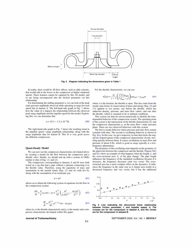
In reality, there would be 3D flow effects, such as eddy currents,that would add to the losses in the compressor at higher rotationalspeeds. These features cannot be captured by this 1D model, andso are being encompassed into the friction parameter via thisrelationship.For determining the stalling parameter α, we can look at the peak
static pressure amplitude observed while operating at surge for eachspeed line in dataset A. The left-hand-side graph in Fig. 7 showshow the value of α impacts the relationship between the observedpeak surge amplitude and the impeller speed for the model. Exploit-ing this, we can determine that
α = 10.3 − 1.5 × 10⁻⁴Ω (60)
The right-hand-side graph in Fig. 7 shows the resulting trend inthe impeller speed—surge amplitude relationship, along with thesurge amplitude data for dataset B. This fit is very good acrossthe different compressors.
Quasi-Steady ModelWe can now use the compressor characteristics developed above
by creating a model for the flow between the compressor and athrottle valve. Ideally, we should end up with a system of ODEssimilar to that of Eqs. (1) and (2).The compressors corresponding to datasets A and B were both
tested on a rig that had a pipe without a plenum connecting it tothe throttle value. Therefore, using the equations of mass andmomentum in the inertial frame (Eqs. (5) and (6) with Ω= 0),along with the assumption of an isentropic gas
p = κργ (61)
allows us to obtain the following system of equations for the flow inthe compression system:
dm
dt=A
L( pc(m) − p) +
κ1/γ
AL
m2
pc(m)1/γ−mT (p)2
p1/γ
( )(62)
dp
dt=γκ1/γ
ALp(γ−1)/γ(m − mT (p)) (63)
where mT is the throttle characteristic and pc is the steady-state com-pressor characteristic developed within this paper.
For the throttle characteristic, we can use
m2T (p) =
2γγ − 1
λ2A2ρρamb
λ2ρ2amb − ρ2
( )(ρpamb − ρambp) (64)
where λ is the fraction, the throttle is open. This has come from thesteady-state forms of conservation of mass and energy (Eqs. (5) and(7)) applied to two points: one before the throttle, which hasunknown density, pressure, and mass flow values, and one afterthe throttle, which is assumed to be at ambient conditions.This system can then be solved numerically to identify the time-
dependent behavior of the compression system. The operating pointof the system is the intersection of the throttle characteristic mT andthe compressor characteristic pc in the mass flow—static pressureplane. There are two observed behaviors with this system.The first is steady behavior where pressure and mass flow remain
constant with time. The second is oscillating behavior as shown inFig. 8(a). In this case, we get a trajectory in time that tracks the neg-atively sloped regions of the compressor characteristic closely, trav-eling quickly between them. It causes oscillations in mass flow andpressure of about 6 Hz, which is good as surge typically is a low-frequency phenomena.The dynamics of this oscillating state depends on the geometry of
the pipework between the compressor and the throttle. Figures 8(b)and 8(c) show an example of what happens when the length, L, andthe cross-sectional area, A, of the pipe change. The pipe lengthinfluences the frequency of the simulated oscillations because if Lincreases, the frequency decreases (and vice versa). The cross-sectional area has a more complex effect on the dynamics. It influ-ences the frequency in the same way as L (larger area results in adecreased frequency and vice versa), but it has the additional
Fig. 5 Diagram indicating the dimensions given in Table 1
Fig. 6 Line indicating the discovered linear relationshipbetween friction parameter, f, and impeller speed, Ω. Thecrosses are for the compressor in dataset A, and the circlesare for the compressor in dataset B.
Journal of Turbomachinery SEPTEMBER 2020, Vol. 142 / 091010-784
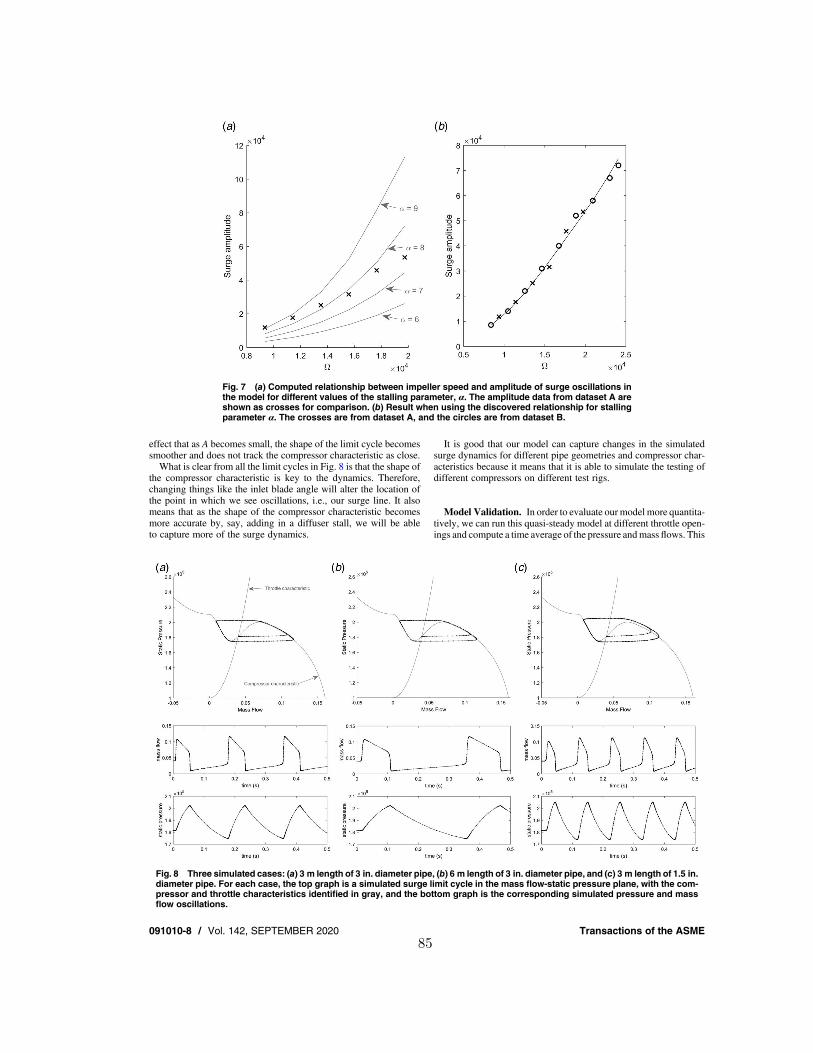
effect that as A becomes small, the shape of the limit cycle becomessmoother and does not track the compressor characteristic as close.What is clear from all the limit cycles in Fig. 8 is that the shape of
the compressor characteristic is key to the dynamics. Therefore,changing things like the inlet blade angle will alter the location ofthe point in which we see oscillations, i.e., our surge line. It alsomeans that as the shape of the compressor characteristic becomesmore accurate by, say, adding in a diffuser stall, we will be ableto capture more of the surge dynamics.
It is good that our model can capture changes in the simulatedsurge dynamics for different pipe geometries and compressor char-acteristics because it means that it is able to simulate the testing ofdifferent compressors on different test rigs.
Model Validation. In order to evaluate our model more quantita-tively, we can run this quasi-steady model at different throttle open-ings and compute a time average of the pressure andmassflows. This
Fig. 7 (a) Computed relationship between impeller speed and amplitude of surge oscillations inthe model for different values of the stalling parameter, α. The amplitude data from dataset A areshown as crosses for comparison. (b) Result when using the discovered relationship for stallingparameter α. The crosses are from dataset A, and the circles are from dataset B.
Fig. 8 Three simulated cases: (a) 3 m length of 3 in. diameter pipe, (b) 6 m length of 3 in. diameter pipe, and (c) 3 m length of 1.5 in.diameter pipe. For each case, the top graph is a simulated surge limit cycle in the mass flow-static pressure plane, with the com-pressor and throttle characteristics identified in gray, and the bottom graph is the corresponding simulated pressure and massflow oscillations.
091010-8 / Vol. 142, SEPTEMBER 2020 Transactions of the ASME85

can be used to produce a time-averaged compressor map, which isessentially what we get through testing. Figure 9 shows this time-averaged map with experimental data points for both datasets Aand B.We have chosen to classify the data into two categories: those
that only show oscillations at the average noise level (whichchanges from about 100 Pa to 1000 Pa, as the impeller speedincreases) are considered steady, and those that show oscillationsgreater than that are considered unsteady. In Fig. 9, we haveplotted the steady data as circles and the unsteady data as crosses.For the simulated compressor map, we have plotted bars that
identify the range of values seen when computing the time-averagesolution. From this, we can see a clear line that indicates the onsetof oscillations in our model. We call this the simulated surge lineand have shown this with comparison to the data underneath eachmap.Our simulated surge line is very close to the local maximum of
the compressor characteristics (see Fig. 4(c)), which is shownwith a gray dashed line in the figure. Since the gradient of the char-acteristic (and hence the location of local maximum and minimum)
is determined by the impeller inlet stall, we can deduce that this stallis triggering our simulated compressor into surge.We can also see that our simulated surge line is close to the
point in the data where it switches from steady behavior to mildoscillation. It appears to predict an earlier surge onset for lowerimpeller speeds, but it is possible that this is due to the fact thatdistinguishing between noise and mild oscillations is difficult forthese points.At high speeds, our surge line is within the region of mild oscil-
lation (or mild surge) and, for compressor A, is getting close to thedeep surge limit (the left-most data point). This suggests that thetrigger for mild surge at these points is likely to be somethingother than impeller inlet stall, and that it is this in combinationwith the impeller inlet stall that causes deep surge.The simulated amplitude of the oscillations is increasing as mass
flow decreases, which is very promising as in experiments, the oscil-lations typically grow toward the deep surge limit (where testing isstopped to prevent damage to the compressor). However, as massflow is reduced, there becomes a point in our simulated map thatthe oscillations stop and the flow becomes stable again. This may
Fig. 9 Comparison between the simulated total-to-total compressor map and the data for datasets Aand B. The simulated map has been plotted as lines with bars showing the max and min simulatedvalues. The data are shown with circles if it is steady and crosses if it showed oscillations larger thanthe average noise level. The speed in krpm is indicated on each line. For clarity, a single speed linefrom the middle of the map is shown separately below. Finally, situated at the bottom, the simulatedsurge line is shown (in solid black) in comparison to the data. The dashed gray line shows the locationof the local maximum of the compressor characteristics (Fig. 4(c)) for comparison.
Journal of Turbomachinery SEPTEMBER 2020, Vol. 142 / 091010-986
indeed be true because Koff and Greitzer [20] found during theirexperimental study of the compressor map that the flow canbecome stable again close to shut-off. However, we have someunsteady data points that lie in this part of our curves, so ourregion of stability is currently larger than is observed experimentally.When examining the fit of the data to the simulated average
total-to-total pressure ratio curves, we can see that for speedsunder 200 krpm, the points follow the steady portion of the curveclosely, and for speeds under 180 krpm, the time-averaged unsteadypoints are also a reasonable fit. From the single speed line plots, it isclear to see that, as mass flow decreases, our model predicts steadyflow behavior with an increasing pressure ratio until the simulatedsurge line, and unsteady flow behavior with a decreasing averagepressure ratio after that point. When the data approach the surgeline, it seems to flatten out instead but usually remains within thesimulated range of oscillation.From the single speed line for dataset B, we can see that the
model is not always able to simulate the pressure ratios for highmass flows. This is because at high mass flows, we approach thechoked flow region, and the Mach number for the flow increasestoward 1. Our model does not include any form of shock loss thatwould occur as the flow approaches the speed of sound, and sodoes not contain all the physics required to capture the chokedflow behavior.Above speeds of 200 krpm, the fit is not as good, meaning that
our model is missing some important physical dynamics for thehigher impeller speeds. Diffuser stall is a phenomenon that isusually triggered first at higher impeller speeds; therefore, incorpo-rating this into the model is expected to improve the fit and surgedynamics at these higher speeds.Overall, this model has been able to predict a surge line for a
compressor by only considering its geometry. There are inaccura-cies in the model, but we have made a choice to compromise onaccuracy for the sake of having a predictive model, and these inac-curacies can be improved upon as more dynamics are added.
Summary and ConclusionsA new method for producing compressor characteristics has been
presented, updating the work on low-dimensional surge modelsdeveloped during the 1970s. An original steady-state compressormodel was developed from the mass, momentum, and energy con-servation laws, along with two factors to model friction and stalling.Creating the model this way allowed for insight into various fea-tures observed in a compressor characteristic. For example, stallingcreates a local minimum and maximum in low forward mass flows.Since the location of this feature correlates to the location of thesurge line in our model, we were able to identify impeller inletstall as a route into surge.The model equations were reduced and simplified to form ODEs
that are quick to solve. If full 3D CFD was used to model flow in acompressor near surge, this highly complex problem becomes verycomputationally expensive. Low-dimensional surge models are aviable alternative because the need for quick evaluations outweighsthe need for high accuracy, and so, it is vital that this speed of com-putation is maintained.Relationships for the friction parameter and stalling parameter
with impeller speed were found by comparison to test data.These relationships hold across multiple compressor geometries,allowing the model to be fully deterministic. Therefore, themodel has the ability to be a predictive tool for surge limits ofnew compressor designs because it only needs geometric measure-ments as inputs.The model showed promising results when compared with com-
pressor map data, and is able to capture reasonably realistic surgefrequencies when included in a low-dimensional surge model. Itis able to identify when oscillations in mass flow and pressure arelikely to appear, and is able to capture a growing amplitude in oscil-lations as the mass flow is further reduced.
Further work is planned to include diffuser recirculation or stallinto this model. It is generally agreed that diffuser stall cantrigger surge at higher impeller speeds, which will hopefullyimprove the accuracy of the model’s surge limit.
AcknowledgmentThe authors are grateful to Tomasz Duda, Stefan Tuechler, and
Zheng Liu, who provided the geometry, compressor map, andsurge amplitude data within this paper.Katherine Powers is supported by a scholarship from the EPSRC
Centre for Doctoral Training in Statistical Applied Mathematics atBath (SAMBa), under the project EP/L015684/1.
NomenclatureMathematical Symbols
f = friction factorg = acceleration due to gravityh = channel heightm = mass flowp = static pressureq = mass flow per radianr = radiusu = velocityA = cross-sectional areaB = Greitzer’s parameterE = specific energyF = frictionL = lengthQ = specific heat energyR = specific gas constantS = surface areaT = temperatureU = specific internal energycv = specific heat at constant volumenb = the number of impeller bladesα = stalling factorβ = flow angleβB = blade angleγ = specific heat ratioκ = isentropic constantλ = fraction throttle is openξT = throttle parameterρ = densityτ = stressΦ = nondimensional mass flowΨ = nondimensional pressureΩ = angular velocity
Subscripts
amb = ambientc = compressorD = diffuserI = impellerr = radial directionT = throttletip = impeller tipx = axial directionθ = tangential direction
References[1] Rasmussen, P. C., and Kurz, R., 2009, “Centrifugal Compressor Applications—
Upstream and Midstream,” Proceedings of the 38th Turbomachinery Symposium,Texas A&M University.
091010-10 / Vol. 142, SEPTEMBER 2020 Transactions of the ASME87

[2] Macdougal, I., and Elder, R. L., 1983, “Simulation of Centrifugal CompressorTransient Performance for Process Plant Applications,” J. Eng. Power, 105(4),pp. 885–890.
[3] Stone, R., 2012, Introduction to Internal Combustion Engines, 4th ed., PalgraveMacMillan, Hampshire, UK.
[4] Watson, N., and Janota, M. S., 1982, Turbocharging: The Internal CombustionEngine, MacMillan, London.
[5] Pampreen, R. C., 1993, Compressor Surge and Stall, Concepts Eti, Norwich, VT.[6] Fink, D. A., Cumpsty, N. A., and Greitzer, E. M., 1992, “Surge Dynamics in a
Free-Spool Centrifugal Compressor System,” ASME J. Turbomach., 114(2),pp. 321–332.
[7] De Jager, B., 1995, “Rotating Stall and Surge Control: A Survey,” Proceedings ofthe 34th IEEE Conference on Decision and Control, New Orleans, LA, Vol. 2, pp.1857–1862.
[8] Longley, J. P., 1994, “A Review of Nonsteady Flow Models for CompressorStability,” ASME J. Turbomach., 116(2), pp. 202–215.
[9] Stenning, A. H., 1980, “Rotating Stall and Surge,” J. Fluid. Eng., 102(1), pp. 14–20.
[10] Linfield, K. W., and Mudry, R. G., 2008, Pros and Cons of CFD and PhysicalFlow Modeling, Airflow Sciences Corporation, Livonia, MI.
[11] Cozzi, L., Rubechini, F., Marconcini, M., Arnone, A., Astrua, P., Schneider, A.,and Silingardi, A., 2017, “Facing the Challenges in CFD Modelling of MultistageAxial Compressors,” ASME Turbo Expo 2017: Turbomachinery TechnicalConference and Exposition, Charlotte, NC.
[12] Arnulfi, G. L., Giannattasio, P., Giusto, C., Massardo, A. F., Micheli, D., andPinamonti, P., 1999, “Multistage Centrifugal Compressor Surge Analysis: PartII—Numerical Simulation and Dynamic Control Parameters Evaluation,”ASME J. Turbomach., 121(2), pp. 312–320.
[13] Van Helvoirt, J., de Jager, B., Steinbuch, M., and Smeulers, J., 2004, “StabilityParameter Identification for a Centrifugal Compression System,” 43rd IEEEConference on Decision and Control, Paradise Islands, The Bahamas, Vol. 4,pp. 3400–3405.
[14] Mizuki, S., Asaga, Y., Ono, Y., and Tsujita, H., 2006, “Investigation ofSurge Behavior in a Micro Centrifugal Compressor,” J. Therm. Sci., 15(2),pp. 97–102.
[15] Tamaki, H., 2008, “Effect of Piping Systems on Surge in CentrifugalCompressors,” J. Mech. Sci. Technol., 2(10), pp. 1857–1863.
[16] Galindo, J., Arnau, F. J., Tiseira, A., and Piqueras, P., 2010, “Solution of theTurbocompressor Boundary Condition for One-Dimensional Gas-DynamicCodes,” Math. Comput. Modell., 52(7–8), pp. 1288–1297.
[17] Torregrosa, A., Arnau, F., Piqueras, P., Reyes-Belmonte, M., Knutsson, M., andLennblad, J., 2012, “Acoustic One-Dimensional Compressor Model forIntegration in a Gas-Dynamic Code,” SAE 2012 World Congress & Exhibition,Detroit, MI.
[18] Greitzer, E. M., 1976, “Surge and Rotating Stall in Axial Flow Compressors—Part I: Theoretical Compression System Model,” J. Eng. Power, 98(2),pp. 190–198.
[19] Hos, C., Champneys, A., and Kullmann, L., 2003, “Bifurcation Analysis of Surgeand Rotating Stall in the Moore-Greitzer Compression System,” IMA J. Appl.Math., 68(2), pp. 205–228.
[20] Koff, S. G., and Greitzer, E. M., 1984, “Stalled Flow Performance for AxialCompressors: I—Axisymmetric Characteristic,” 29th International Gas TurbineConference and Exhibit, Amsterdam, Netherlands.
[21] Galindo, J., Serrano, J. R., Climent, H., and Tiseira, A., 2008, “Experiments andModelling of Surge in Small Centrifugal Compressor for Automotive Engines,”Exp. Therm. Fluid. Sci., 32(3), pp. 818–826.
[22] Moore, F. K., and Greitzer, E. M., 1986, “A Theory of Post-Stall Transients inAxial Compression Systems: Part I—Development of Equations,” ASMEJ. Eng. Gas Turb. Power, 108(1), pp. 68–76.
[23] Zagorowska, M., and Thornhill, N. F., 2017, “Compressor Map ApproximationUsing Chebyshev Polynomials,” 25th Mediterranean Conference on Controland Automation (MED), Valletta, Malta, pp. 846–869.
[24] Li, X., Yang, C., Wang, Y., and Wang, H., 2018, “A Prediction Model ofCompressor With Variable-Geometry Diffuser Based on Elliptic Equation andPartial Least Squares,” R. Soc. Open Sci., 5(1), pp. 1–19.
[25] Elder, R. L., and Gill, M. E., 1985, “A Discussion of the Factors AffectingSurge in Centrifugal Compressors,” ASME J. Eng. Gas Turb. Power, 107(2),pp. 499–506.
[26] Martin, G., Talon, V., Higelin, P., Charlet, A., and Caillol, C., 2009,“Implementing Turbomachinery Physics Into Data Map-Based TurbochargerModels,” SAE Int. J. Engines, 2(1), pp. 211–229.
[27] Japikse, D., 1996, Centrifugal Compressor Design and Performance, Vol. 2,Concepts Eti, White River Junction, VT.
[28] Velasquez, E. I. G., 2017, “Determination of a Suitable Set of Loss Models forCentrifugal Compressor Performance Prediction,” Chinese J. Aeronaut., 30(5),pp. 1644–1650.
[29] Oh, H. W., Yoon, E. S., and Chung, M. K., 1997, ““An Optimum Set of LossModels for Performance Prediction of Centrifugal Compressors,” Proc. Inst.Mech. Eng. Part A: J. Power Energy, 211(4), pp. 331–338.
[30] Gong, X., and Chen, R., 2014, “Total Pressure Loss Mechanism of CentrifugalCompressors,” Mech. Eng. Res., 4(2), pp. 45–59.
[31] Burr, K. P., Akylas, T. R., and Mei, C. C., 2003, Chapter 2: Two-DimensionalLaminar Boundary Layers, Lecture Notes, MIT, Cambridge, MA.
[32] Winterbone, D. E., and Pearson, R. J., 2000, Theory of Engine ManifoldDesign: Wave Action Methods for I.C. Engines, Professional EngineeringPublishing, London, UK.
[33] Day, I. J., Greitzer, E. M., and Cumpsty, N. A., 1978, “Prediction of CompressorPerformance in Rotating Stall,” J. Eng. Power, 100(1), pp. 1–12.
Journal of Turbomachinery SEPTEMBER 2020, Vol. 142 / 091010-1188
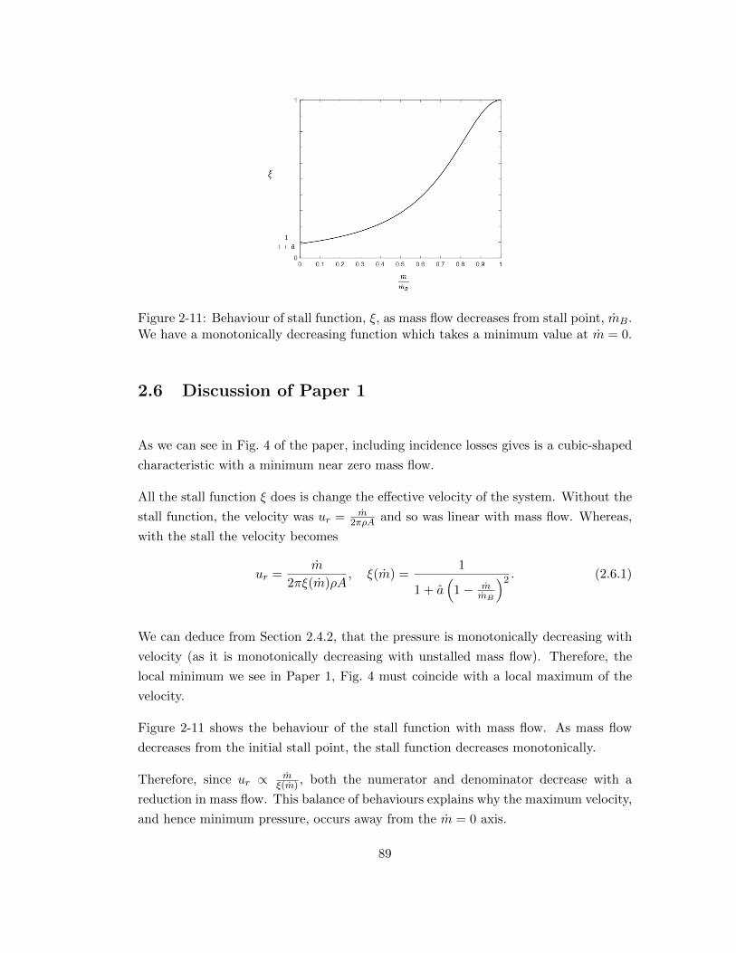
Figure 2-11: Behaviour of stall function, ξ, as mass flow decreases from stall point, mB.We have a monotonically decreasing function which takes a minimum value at m = 0.
2.6 Discussion of Paper 1
As we can see in Fig. 4 of the paper, including incidence losses gives is a cubic-shaped
characteristic with a minimum near zero mass flow.
All the stall function ξ does is change the effective velocity of the system. Without the
stall function, the velocity was ur = m2πρA and so was linear with mass flow. Whereas,
with the stall the velocity becomes
ur =m
2πξ(m)ρA, ξ(m) =
1
1 + a(
1− mmB
)2 . (2.6.1)
We can deduce from Section 2.4.2, that the pressure is monotonically decreasing with
velocity (as it is monotonically decreasing with unstalled mass flow). Therefore, the
local minimum we see in Paper 1, Fig. 4 must coincide with a local maximum of the
velocity.
Figure 2-11 shows the behaviour of the stall function with mass flow. As mass flow
decreases from the initial stall point, the stall function decreases monotonically.
Therefore, since ur ∝ mξ(m) , both the numerator and denominator decrease with a
reduction in mass flow. This balance of behaviours explains why the maximum velocity,
and hence minimum pressure, occurs away from the m = 0 axis.
89

Furthermore, as was shown in Paper 1, Fig. 8, this new shape of characteristic can
simulate surge-like behaviour when combined with the nonlinear reduced order model
presented in Section 2.2.
This surge-like behaviour coincides with the positive gradient of the compressor charac-
teristic (between the local minimum (a) and local maximum (c) as labelled in Paper 1,
Fig. 4). This positive gradient only occurs because of our inclusion of incidence losses
into the model. Therefore, incidence loss and the resulting impeller inlet stall is a vital
mechanism for surge.
As we can see from Paper 1, Fig. 8, the mass flow oscillations stay positive for all time.
Therefore this is technically classed as mild surge. However, the simulated amplitudes
of oscillation imply this should be deep surge. This means that the current stall function
may not be using the correct assumptions.
2.6.1 Improvement of Stall Function
From Paper 1, Fig. 8, it appears that the intercept value is too high for our limit cycles
to enter the negative flow regime. The limit cycle appears to retain an almost constant
pressure from the local maximum until it intersects the characteristic just before the
axis. If the intercept value was lower, then it’s possible for the limit cycle to enter the
negative mass flow region before intersecting the characteristic.
This implies that we may have had the wrong condition at m = 0. Since m = 2πξAρur,
we assumed that m = 0 results in ur = 0. However, there is the possibility that ξ = 0
instead. This would mean that at zero flow, incidence losses are at a maximum as the
entire impeller channel has stalled. This agrees with the suggestion from Watson and
Janota [1] shown in Fig. 2-9 where the incidence losses increase monotonically from the
optimal case of flow angle matching the blade angle.
In Section 2.4.3 we derived the form of the stall function using
m
ξAρ= ur(m) = am3 + bm2 + cm+ d. (2.6.2)
By no longer requiring ur = 0 at m = 0, we do not assume d = 0, but the other
90
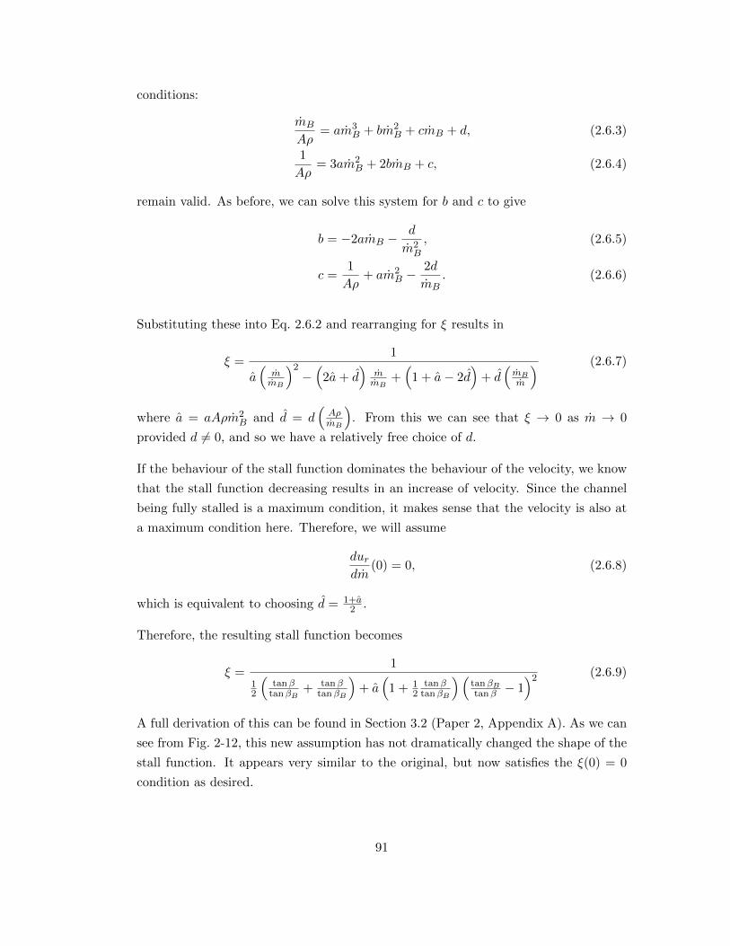
conditions:
mB
Aρ= am3
B + bm2B + cmB + d, (2.6.3)
1
Aρ= 3am2
B + 2bmB + c, (2.6.4)
remain valid. As before, we can solve this system for b and c to give
b = −2amB −d
m2B
, (2.6.5)
c =1
Aρ+ am2
B −2d
mB. (2.6.6)
Substituting these into Eq. 2.6.2 and rearranging for ξ results in
ξ =1
a(mmB
)2−(
2a+ d)
mmB
+(
1 + a− 2d)
+ d(mBm
) (2.6.7)
where a = aAρm2B and d = d
(AρmB
). From this we can see that ξ → 0 as m → 0
provided d 6= 0, and so we have a relatively free choice of d.
If the behaviour of the stall function dominates the behaviour of the velocity, we know
that the stall function decreasing results in an increase of velocity. Since the channel
being fully stalled is a maximum condition, it makes sense that the velocity is also at
a maximum condition here. Therefore, we will assume
durdm
(0) = 0, (2.6.8)
which is equivalent to choosing d = 1+a2 .
Therefore, the resulting stall function becomes
ξ =1
12
(tanβ
tanβB+ tanβ
tanβB
)+ a
(1 + 1
2tanβ
tanβB
)(tanβBtanβ − 1
)2 (2.6.9)
A full derivation of this can be found in Section 3.2 (Paper 2, Appendix A). As we can
see from Fig. 2-12, this new assumption has not dramatically changed the shape of the
stall function. It appears very similar to the original, but now satisfies the ξ(0) = 0
condition as desired.
91

Figure 2-12: Behaviour of revised stall function, ξ, as mass flow decreases from stallpoint, mB. We have a monotonically decreasing function which satisfies ξ(0) = 0.
Figure 2-13 shows the compressor characteristics if we use this new stall function. We
observe that we have a discontinuity at zero flow. This is problematic because it is
unclear how we should define the compressor characteristic at m = 0. Furthermore,
numerical software for solving ODEs can have problems resolving discontinuities so
special care would need to be taken around this point. (See Gear and Osterby [58] for
a discussion of solving ODEs with discontinuities.)
To understand why we have a discontinuity, recall (from Eq.2.4.69 and 2.4.72) that we
Figure 2-13: Resulting compressor characteristic for new stall function. A discontinuityoccurs at m = 0 due to a jump in velocity at this point.
92

have
p =γ − 1
γ
(EIρ−
ρu2r
2+ρΩ2r2
2
)(2.6.10)
p =γ − 1
γ
(EDρ−
ρu2r
2− u2
θ
2
)(2.6.11)
in the impeller and diffuser respectively.
The new stall function implies that at m = 0 we have a velocity ur 6= 0 as ξ = 0.
However, in reverse flow we have no stall function and so ur = 0 at zero flow. This
jump in velocity explains the jump in pressure.
As we saw in Section 1.2.1, all the previously proposed compressor characteristics have
been smooth with no discontinuities. If we believe this to hold for our characteristic,
then that means energy is lost in some way in the reverse flow regime so that EI and
ED can balance the jump in velocity at zero flow.
Therefore, it is worth taking a more detailed look into the behaviour of flow travelling
in the reversed direction through the compressor. This is the topic of the next chapter.
2.7 Conclusions
In this chapter, we have derived a reduced order model for compressor surge, along
with a throttle and compressor characteristic.
Through the derivation of the steady-state compressor characteristic, we have learned
that friction and incidence losses are key dynamics in order to achieve realistic simula-
tions of a compressor.
Since we have developed loss functions to incorporate the dynamics of friction and
impeller inlet stall, the resulting model depends on two parameters that control the
strength of these losses. In order for this model to be fully predictive, universal rela-
tions need to be found for these parameters. Paper 1 found some relations that are
promising, however due to limits of the amount of available data, we cannot conclude
these relations will hold universally across a variety of compressor sizes.
In Paper 1, we also observed that our model may be too simplistic to predict the surge
line accurately for all impeller speeds. We saw that our model was predicting surge
onset at lower mass flows than the experimental data suggested for the higher impeller
93
speeds, and deduced that the inclusion of diffuser recirculation may be needed.
We also noticed that our current model was only capturing mild surge dynamics as
the mass flows remained positive for all times, despite the pressure oscillations having
amplitudes reminiscent of deep surge.
We have proposed an alternative stall function that assumes the impeller channels
are fully stalled at zero flow. This gives a more promising shape of characteristic for
m > 0. However, it results in a discontinuity at m = 0 and so we concluded that a
more detailed look into reverse flow was required.
94
Chapter 3
Reverse Flow Region in
Compressor Characteristics
As we discovered in Section 2.6.1, it is important to consider the dynamics of flow
travelling backwards through the compressor. This is an area of research that tends
to be overlooked, but it is important as the shape of the characteristic for m < 0 will
influence the behaviour of deep surge cycles.
3.1 Reverse Flow Model Development
From now on, we will construct the compressor characteristic by two separate models.
The first will be the model developed in the previous chapter, with the new stall
function suggested in Section 2.6.1, for positive mass flows. The second we will develop
in this chapter and will be for negative mass flows.
Figure 3-1 shows how the model developed in Section 2.5 modelled reversed flow. These
are plots with radius so they need to be read from right to left (as the flow is travelling
from the diffuser outlet to the impeller inlet).
There are two main points to note. Firstly, the direction of flow in the diffuser does
not follow the shape of the volute. Instead it is in the same direction as positive flow.
Secondly, the tangential velocity is increasing monotonically until it matches the speed
of the impeller at the impeller-diffuser interface.
95
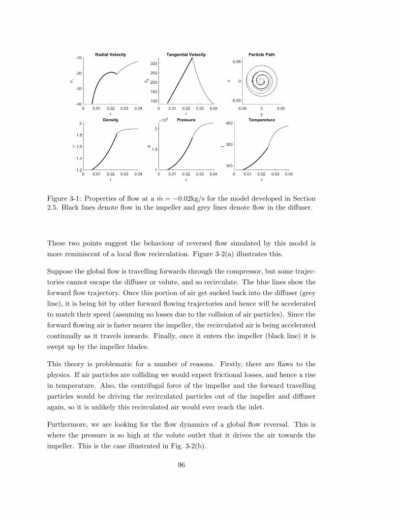
Figure 3-1: Properties of flow at a m = −0.02kg/s for the model developed in Section2.5. Black lines denote flow in the impeller and grey lines denote flow in the diffuser.
These two points suggest the behaviour of reversed flow simulated by this model is
more reminiscent of a local flow recirculation. Figure 3-2(a) illustrates this.
Suppose the global flow is travelling forwards through the compressor, but some trajec-
tories cannot escape the diffuser or volute, and so recirculate. The blue lines show the
forward flow trajectory. Once this portion of air get sucked back into the diffuser (grey
line), it is being hit by other forward flowing trajectories and hence will be accelerated
to match their speed (assuming no losses due to the collision of air particles). Since the
forward flowing air is faster nearer the impeller, the recirculated air is being accelerated
continually as it travels inwards. Finally, once it enters the impeller (black line) it is
swept up by the impeller blades.
This theory is problematic for a number of reasons. Firstly, there are flaws to the
physics. If air particles are colliding we would expect frictional losses, and hence a rise
in temperature. Also, the centrifugal force of the impeller and the forward travelling
particles would be driving the recirculated particles out of the impeller and diffuser
again, so it is unlikely this recirculated air would ever reach the inlet.
Furthermore, we are looking for the flow dynamics of a global flow reversal. This is
where the pressure is so high at the volute outlet that it drives the air towards the
impeller. This is the case illustrated in Fig. 3-2(b).
96
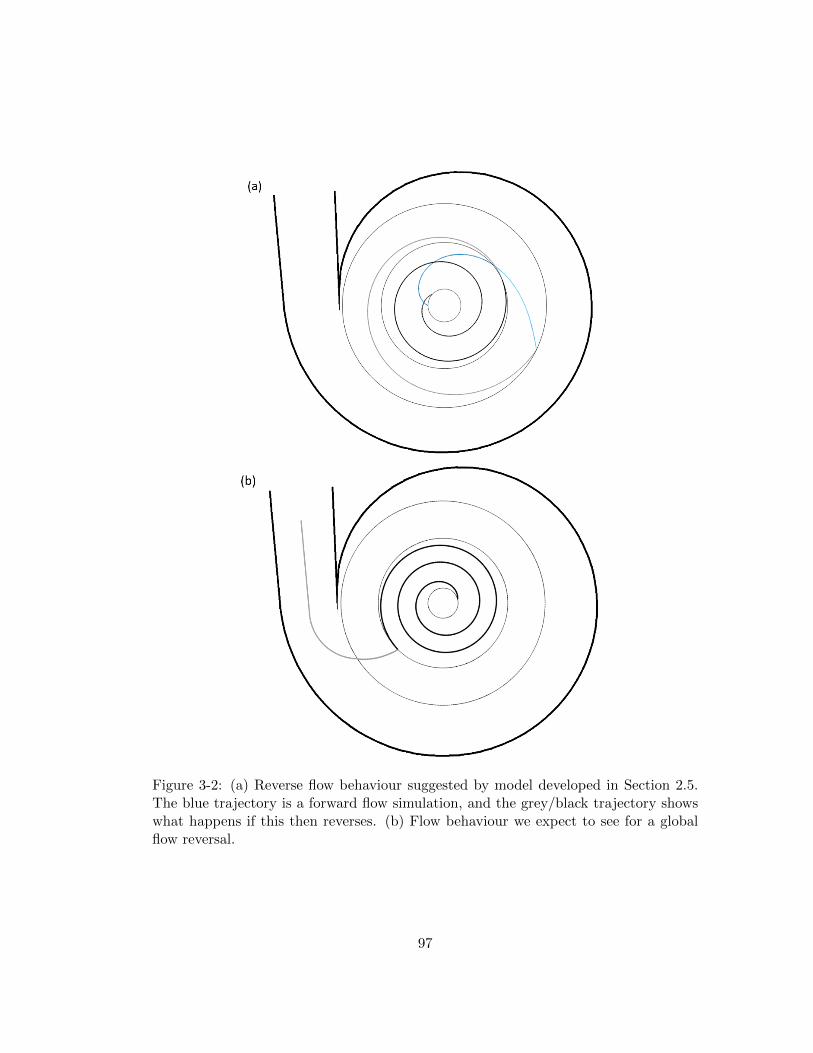
Figure 3-2: (a) Reverse flow behaviour suggested by model developed in Section 2.5.The blue trajectory is a forward flow simulation, and the grey/black trajectory showswhat happens if this then reverses. (b) Flow behaviour we expect to see for a globalflow reversal.
97

In order to simulate this global flow reversal, a different boundary condition needs to be
used for tangential velocity. The previous model assumed that the tangential velocity
at the impeller-diffuser interface would be equal to that of the rotating impeller, but
this need not be the case. Instead we will look for a boundary condition that depends
on the shape of the volute so we know at what angle the flow would enter the diffuser.
Moreover, noticing that we expect there to be a large a jump in tangential velocity at
the impeller-diffuser interface, we can expect shear losses to play an important role for
reverse flow. These shear losses would provide a way to balance the pressure drop at
m = 0 seen in forward flow due to the new stall function (presented in Section 2.6.1).
The paper in the next section derives a new model for reversed flow, including the two
main changes suggested above. It also presents the resulting compressor characteristics
and compares them with experimental data for the reversed flow regime.
98

This declaration concerns the article entitled:
Development and Validation of a Model for Centrifugal Compressors in Reversed Flow Regimes
Publication status (tick one)
Draft manuscript Submitted In review Accepted Published X
Publication details (reference)
Powers, K., Kennedy, I., Brace, C., Milewski P., and Copeland, C. (January 11, 2021) “Development and Validation of a Model for Centrifugal Compressors in Reversed Flow Regimes.” Proceedings of the ASME Turbo Expo 2020: Turbomachinery Technical Conference and Exposition. ASME. https://doi.org/10.1115/GT2020-16005
Copyright status (tick the appropriate statement)
I hold the copyright for this material Copyright is retained by the publisher, but I have
been given permission to replicate the material here X
Candidate’s contribution to the paper (provide details, and also indicate as a percentage)
The contribution of Katherine Powers to the paper is as follows:
• Formulation of ideas (90%) with advice from supervising authors
• Derivation of equations for the mathematical models (90%)
• Participation in design and implementation of experiments (40%)
• Writing MATLAB code and creating of numerical simulations (100%)
• Comparing numerical simulations to given experimental data, and analysing of the results (100%)
• Presentation of data in journal format (90%)
Statement from Candidate
This paper reports on original research I conducted during the period of my Higher Degree by Research candidature.
Signed
Date
26/02/2021
3.2 Paper 2: Development and Validation of a Model for
Centrifugal Compressors in Reversed Flow Regimes
99
Proceedings of ASME Turbo Expo 2020Turbomachinery Technical Conference and Exposition
GT2020June 22-26, 2020, London, England
GT2020-16005
DEVELOPMENT AND VALIDATION OF A MODEL FOR CENTRIFUGALCOMPRESSORS IN REVERSED FLOW REGIMES
Katherine H. Powers, Ian J. Kennedy, Chris J. Brace, Paul A. Milewski, Colin D. CopelandUniversity of Bath
Claverton Down, Bath, BA2 7AY. UKEmail: [email protected]
ABSTRACT
Turbochargers are widely used to help reduce the environ-mental impact of automotive engines. However, a limiting factorfor turbochargers is compressor surge. Surge is an instabilitythat induces pressure and flow oscillations that often damagesthe turbocharger and its installation.
Most predictions of the surge limit are based on low-ordermodels, such as the Moore-Greitzer model. These models tend torely on a characteristic curve for the compressor created by ex-trapolating the constant speed lines of a steady-state compressormap into the negative mass flow region. However, there is littlevalidation of these assumptions in the public literature.
In this paper, we develop further the first-principles modelfor a compressor characteristic presented in Powers et al. [1],with a particular emphasis on reverse flow. We then perform ex-periments using a 58mm diameter centrifugal compressor pro-vided by Cummins Turbo Technologies, where we feed air inthe reverse direction though the compressor while the impelleris spinning in the forwards direction in order to obtain data inthe negative mass flow region of the compressor map.
This demonstrated experimentally that there is a stable op-erating region in the reverse flow regime. The recorded datashowed a good match with the theoretical model developed inthis paper. We also identified a change in characteristic be-haviour as the impeller speed is increased which, to the authorsknowledge, has not been observed in any previously publishedexperimental work.
NOMENCLATUREA Cross-sectional areaa Stalling factorB Greitzer’s parameterdet DeterminantE Specific energyf Friction factorF Skin frictiong Acceleration due to gravityh Channel heightJ JacobianL Lengthm Mass flownb Number of impeller bladesp Static pressureQ Heat transferq Mass flow per radianR Specific gas constantS Surface area per unit volumeT Temperaturetr Traceu Velocityβ Flow angleβB Blade angleδ Thickness of shear layerγ Specific heat ratioκ Isentropic constantλ Second viscosity coefficientµ Dynamic viscosity
1 Copyright c© 2020 by ASME
100
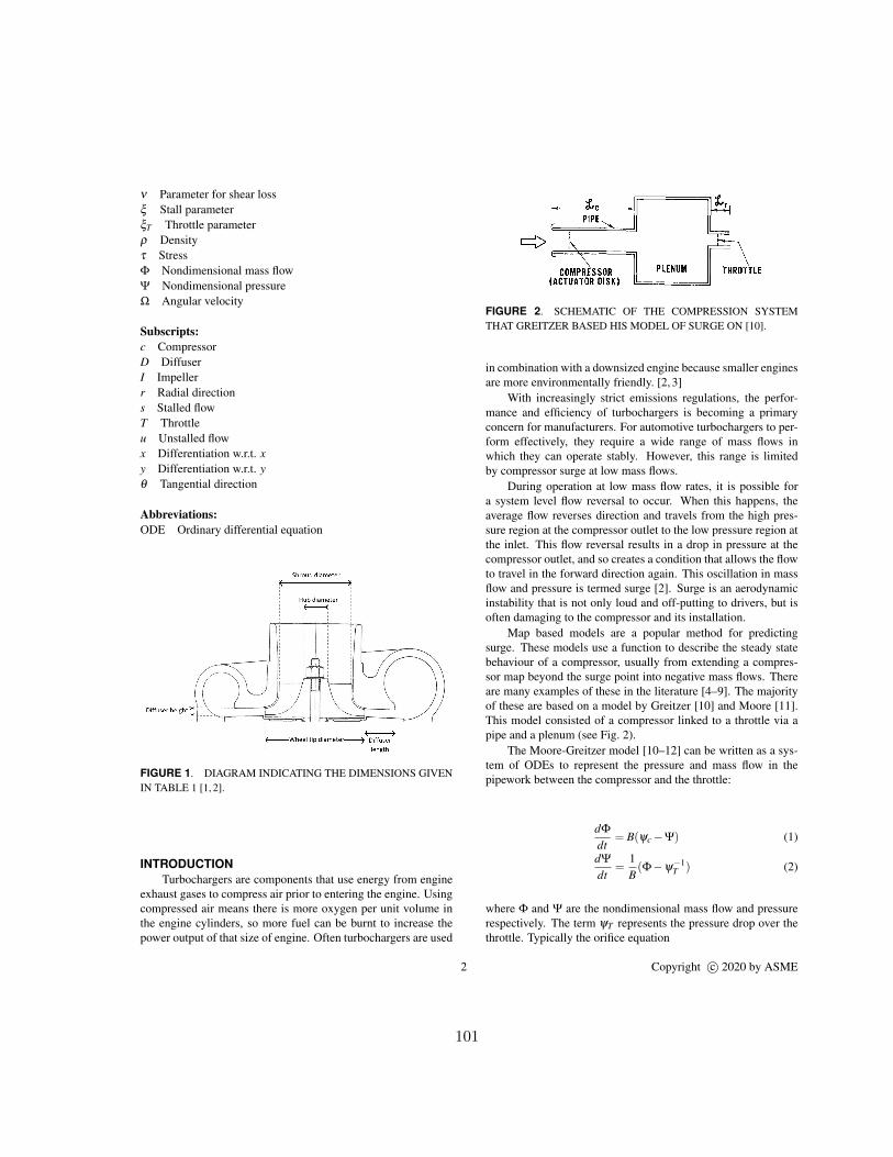
ν Parameter for shear lossξ Stall parameterξT Throttle parameterρ Densityτ StressΦ Nondimensional mass flowΨ Nondimensional pressureΩ Angular velocity
Subscripts:c CompressorD DiffuserI Impellerr Radial directions Stalled flowT Throttleu Unstalled flowx Differentiation w.r.t. xy Differentiation w.r.t. yθ Tangential direction
Abbreviations:ODE Ordinary differential equation
FIGURE 1. DIAGRAM INDICATING THE DIMENSIONS GIVENIN TABLE 1 [1, 2].
INTRODUCTIONTurbochargers are components that use energy from engine
exhaust gases to compress air prior to entering the engine. Usingcompressed air means there is more oxygen per unit volume inthe engine cylinders, so more fuel can be burnt to increase thepower output of that size of engine. Often turbochargers are used
FIGURE 2. SCHEMATIC OF THE COMPRESSION SYSTEMTHAT GREITZER BASED HIS MODEL OF SURGE ON [10].
in combination with a downsized engine because smaller enginesare more environmentally friendly. [2, 3]
With increasingly strict emissions regulations, the perfor-mance and efficiency of turbochargers is becoming a primaryconcern for manufacturers. For automotive turbochargers to per-form effectively, they require a wide range of mass flows inwhich they can operate stably. However, this range is limitedby compressor surge at low mass flows.
During operation at low mass flow rates, it is possible fora system level flow reversal to occur. When this happens, theaverage flow reverses direction and travels from the high pres-sure region at the compressor outlet to the low pressure region atthe inlet. This flow reversal results in a drop in pressure at thecompressor outlet, and so creates a condition that allows the flowto travel in the forward direction again. This oscillation in massflow and pressure is termed surge [2]. Surge is an aerodynamicinstability that is not only loud and off-putting to drivers, but isoften damaging to the compressor and its installation.
Map based models are a popular method for predictingsurge. These models use a function to describe the steady statebehaviour of a compressor, usually from extending a compres-sor map beyond the surge point into negative mass flows. Thereare many examples of these in the literature [4–9]. The majorityof these are based on a model by Greitzer [10] and Moore [11].This model consisted of a compressor linked to a throttle via apipe and a plenum (see Fig. 2).
The Moore-Greitzer model [10–12] can be written as a sys-tem of ODEs to represent the pressure and mass flow in thepipework between the compressor and the throttle:
dΦdt
= B(ψc−Ψ) (1)
dΨdt
=1B(Φ−ψ−1
T ) (2)
where Φ and Ψ are the nondimensional mass flow and pressurerespectively. The term ψT represents the pressure drop over thethrottle. Typically the orifice equation
2 Copyright c© 2020 by ASME
101

FIGURE 3. CUBIC FUNCTION AND ITS PARAMETERISATIONTHAT MOORE AND GREITZER USED AS A COMPRESSORCHARACTERISTIC [11].
ψT = ξT 0 +1
ξ 2T
Φ2, (3)
[12] is used.The term ψc is the compressor characteristic, which repre-
sents the pressure rise over the compressor in steady-state con-ditions. This characteristic is difficult to determine. Koff andGreitzer [13] performed an experimental study on an axial com-pressor to determine its shape. They discovered that it was ap-proximately cubic, so Moore and Greitzer [11] proposed using acubic polynomial with parameters that can be fitted to compres-sor map data, i.e.
ψc = ψc0 +H
[1+
23
(ΦW−1)− 1
2
(ΦW−1)3]
(4)
where the parameters are explained in Fig. 3. In 2008, Galindoet al. [14] did a similar experimental study for a small centrifugalcompressor, also producing a cubic-like curve.
Since the compressor map data is contained within the pos-itive mass flow region, using a cubic effectively extrapolates thetrend into the negative flow region, meaning error can easily beinduced here.
There have been some more theoretical approaches to deter-mine the compressor characteristic. The majority of those seenin the literature have involved mean-line or lumped parametermodelling, e.g. [15–17], but recently Powers et al. [1] developeda model from first principles. However, there is little evidenceto validate these compressor characteristics in the reverse flowregime.
The reverse flow region is important because it contributesto the behaviour of the flow during deep surge cycles. Therefore,understanding the physics in the reversed flow region better couldhelp us understand the nature of surge cycles and help mitigatetheir damaging behaviour.
Also, a more accurate representation of reverse flow will im-prove the accuracy of surge models. Surge models are vital forturbocharger and engine designers because they need to under-stand the operating regimes of the turbocharger and, more specif-ically, the limits in which they can operate safely.
The aim of this paper is to perform a more detailed study intothe reversed flow region of the compressor characteristic. Firstly,we will further develop the model presented by Powers et al. [1],taking more care over the reversed flow region. Then we willperform experiments using a 58mm compressor in order to mapthis region and look at how the characteristic shape changes overdifferent operating regimes. Finally, we will compare the experi-mental results to physical models for compressor characteristics,focusing in particular on the model developed here.
MATHEMATICAL MODELPowers et al. [1] developed a model for the compressor char-
acteristics starting from the fundamental equations for conserva-tion of mass, momentum (in a rotating frame) and energy:
∂ρ∂ t
+∇ · (ρu) = 0, (5)
∂∂ t (ρu)+∇ · (ρ(u⊗u))+2ρ(ΩΩΩ×u)+ρ(ΩΩΩ× (ΩΩΩ× r)) = ρg−∇p+∇ · τ, (6)∂∂ t
(ρE)+∇ · (ρuE + pu)−∇ · (τ ·u) = ρQ (7)
respectively, along with the ideal gas law p = ρRT and the as-sumption of a perfect gas (so the specific heat ratio, γ , is assumedconstant).
This was reduced to a system of 1D ODEs in the radial di-rection by assuming:
(i) radial impeller blades, so uθ = 0 in the rotating frame, and(ii) a vaneless diffuser with axisymmetric flow, so ∂
∂θ = 0,
and then averaging over the axial direction.The resulting ODEs for the impeller were
1r
∂∂ r
(rhρur) = 0, (8)
1r
∂∂ r
(rhρu2r )−hρΩ2r =−h
∂ p∂ r
+hFr, (9)
1r
∂∂ r
(rhρur
(u2
r
2+
γγ−1
pρ− Ω2r2
2
))= 0, (10)
3 Copyright c© 2020 by ASME
102

and for the diffuser were
1r
∂∂ r
(rhρur) = 0, (11)
1r
∂∂ r
(rhρu2r )−
hρu2θ
r=−h
∂ p∂ r
+hFr, (12)
1r
∂∂ r
(rhρuruθ )+hρuruθ
r= hFθ , (13)
1r
∂∂ r
(rhρur
(u2
r
2+
u2θ2
+γ
γ−1pρ
))= 0, (14)
where
Fr =f2
ρu2r S (15)
Fθ =f2
ρuruθ S (16)
represent skin friction.A relationship for the friction parameter was found from per-
forming a least squares fit to data:
f = 0.14+5×10⁻⁶Ω. (17)
This was validated against different compressor geometries toshow its potential as a universal relationship.
Powers et al. [1] also created a stall function to take intoaccount how the compressor responds to incidence losses andany resulting local recirculation. We have deviated from theirwork and propose a new stall function, ξ .
Writing
m = ξ Aρur, (18)
we see that ξ A represents the area of the channel that is notblocked due to stall. Therefore, at ξ = 1 the flow is not stalledand at ξ = 0 the flow is completely stalled.
We shall assume that, like Powers et al., when the flow stalls,the velocity is continuous with a continuous gradient. However,instead of forcing the unstalled flow velocity to be zero at zeromass flow, we shall assume that the velocity of the unstalled flowincreases with stalling and will be a maximum when the systemis fully stalled.
It may sound counter-intuitive to allow a non-zero velocityfor the unstalled portion of the flow when the average flow iszero. However, let subscripts u and s denote unstalled and stalledportions respectively, then
m = Asρ>0
us + 0
Auρuu = 0. (19)
FIGURE 4. RELATIONSHIP BETWEEN IMPELLER SPEED ANDDEEP SURGE AMPLITUDE FOR STALL PARAMETER a = 1.7.TEST DATA INDICATED AS CIRCLES HAS BEEN ADDED FORCOMPARISON.
This shows us that at m = 0, all of the flow is stalled and so havean average velocity of zero, and none of the flow is unstalled soit is a valid to have a non-zero velocity at that point.
These assumptions result in
ξ =1
12
(tanβBtanβ + tanβ
tanβB
)+ a(
1+ 12
tanβtanβB
)(tanβBtanβ −1
)2 , (20)
where a is the parameter that controls the level of stalling (seeAppendix A for full derivation).
Since this is a different function to the stall parameter fromPowers et al. we cannot use their correlation. Surge tests wereperformed using the same turbocharger as in the reverse flowtests below. Using the amplitude of the pressure oscillations dur-ing a deep surge cycle, we determined that a = 1.7 for this com-pressor (see Fig. 4). Unlike Powers et al. this is not a universalrelation and so further work is needed to develop a relationshipfor the stall parameter so the model developed can remain pre-dictive.
The stall function created by Powers et al. [1] had a localminimum in the positive flow region, which implied that the flowwould recover from surge and be stable at a low enough forwardmass flow. However, this new function effectively shifts the lo-cal minimum in the characteristic so that it is at zero mass flow,meaning that, once the flow is surging, it will continue to surgeas the mass flow is reduced to zero, and only once the flow isreversed will it stabilise.
Reverse flowWe shall now make a few small changes to this model to
make it suitable for the reverse flow case. First, it is important to
4 Copyright c© 2020 by ASME
103
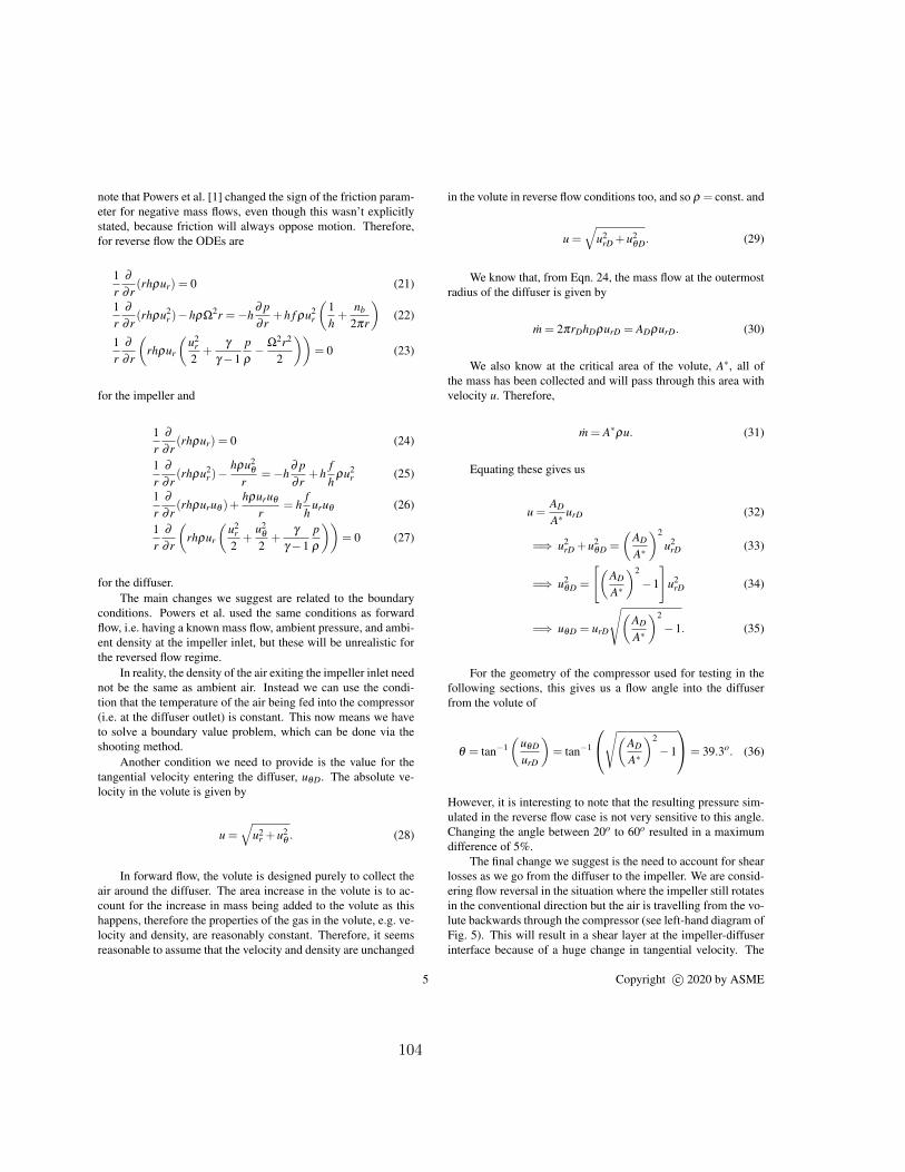
note that Powers et al. [1] changed the sign of the friction param-eter for negative mass flows, even though this wasn’t explicitlystated, because friction will always oppose motion. Therefore,for reverse flow the ODEs are
1r
∂∂ r
(rhρur) = 0 (21)
1r
∂∂ r
(rhρu2r )−hρΩ2r =−h
∂ p∂ r
+h f ρu2r
(1h+
nb
2πr
)(22)
1r
∂∂ r
(rhρur
(u2
r
2+
γγ−1
pρ− Ω2r2
2
))= 0 (23)
for the impeller and
1r
∂∂ r
(rhρur) = 0 (24)
1r
∂∂ r
(rhρu2r )−
hρu2θ
r=−h
∂ p∂ r
+hfh
ρu2r (25)
1r
∂∂ r
(rhρuruθ )+hρuruθ
r= h
fh
uruθ (26)
1r
∂∂ r
(rhρur
(u2
r
2+
u2θ2
+γ
γ−1pρ
))= 0 (27)
for the diffuser.The main changes we suggest are related to the boundary
conditions. Powers et al. used the same conditions as forwardflow, i.e. having a known mass flow, ambient pressure, and ambi-ent density at the impeller inlet, but these will be unrealistic forthe reversed flow regime.
In reality, the density of the air exiting the impeller inlet neednot be the same as ambient air. Instead we can use the condi-tion that the temperature of the air being fed into the compressor(i.e. at the diffuser outlet) is constant. This now means we haveto solve a boundary value problem, which can be done via theshooting method.
Another condition we need to provide is the value for thetangential velocity entering the diffuser, uθD. The absolute ve-locity in the volute is given by
u =√
u2r +u2
θ . (28)
In forward flow, the volute is designed purely to collect theair around the diffuser. The area increase in the volute is to ac-count for the increase in mass being added to the volute as thishappens, therefore the properties of the gas in the volute, e.g. ve-locity and density, are reasonably constant. Therefore, it seemsreasonable to assume that the velocity and density are unchanged
in the volute in reverse flow conditions too, and so ρ = const. and
u =√
u2rD +u2
θD. (29)
We know that, from Eqn. 24, the mass flow at the outermostradius of the diffuser is given by
m = 2πrDhDρurD = ADρurD. (30)
We also know at the critical area of the volute, A∗, all ofthe mass has been collected and will pass through this area withvelocity u. Therefore,
m = A∗ρu. (31)
Equating these gives us
u =AD
A∗urD (32)
=⇒ u2rD +u2
θD =
(AD
A∗
)2
u2rD (33)
=⇒ u2θD =
[(AD
A∗
)2
−1
]u2
rD (34)
=⇒ uθD = urD
√(AD
A∗
)2
−1. (35)
For the geometry of the compressor used for testing in thefollowing sections, this gives us a flow angle into the diffuserfrom the volute of
θ = tan−1(
uθD
urD
)= tan−1
√(
AD
A∗
)2
−1
= 39.3o. (36)
However, it is interesting to note that the resulting pressure sim-ulated in the reverse flow case is not very sensitive to this angle.Changing the angle between 20o to 60o resulted in a maximumdifference of 5%.
The final change we suggest is the need to account for shearlosses as we go from the diffuser to the impeller. We are consid-ering flow reversal in the situation where the impeller still rotatesin the conventional direction but the air is travelling from the vo-lute backwards through the compressor (see left-hand diagram ofFig. 5). This will result in a shear layer at the impeller-diffuserinterface because of a huge change in tangential velocity. The
5 Copyright c© 2020 by ASME
104
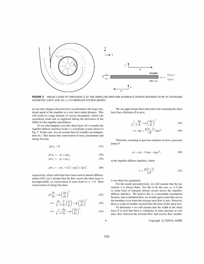
FIGURE 5. SHEAR LAYER OF THICKNESS δ AT THE IMPELLER-DIFFUSER INTERFACE DURING REVERSE FLOW IN STANDARDGEOMETRY (LEFT) AND AN x-y CO-ORDINATE SYSTEM (RIGHT).
air not only changes direction but is accelerated to the large rota-tional speed of the impeller in a very short radial distance. Thiswill result in a large amount of viscous dissipation, which wasconsidered small and so neglected during the derivation of theODEs for the impeller and diffuser.
To see what happens over this shear layer, let’s consider theimpeller-diffuser interface in the x-y coordinate system shown inFig. 5. In this case, we can assume that all variables are indepen-dent of x. This means that conservation of mass, momentum andenergy become
(ρv)y = 0 (37)
ρvuy =−px +µuyy (38)ρvvy =−py +µvyy (39)
ρvey =−pvy +λv2y +µu2
y +2µv2y (40)
respectively, where subscripts have been used to denote differen-tiation [18]. Let’s assume that the flow across the shear layer isincompressible, so conservation of mass leads to vy = 0. Thenconservation of energy becomes
ρv∂e∂y
= µ(
∂u∂y
)2
(41)
=⇒ ρvγ−1
∂∂y
(pρ
)= µ
(∂u∂y
)2
(42)
=⇒ vγ−1
∂ p∂y
= µ(
∂u∂y
)2
. (43)
We can approximate these derivatives by assuming the shearlayer has a thickness δ to give,
vγ−1
∆pδ
= µ(
∆uδ
)2
(44)
=⇒ ∆p =µ(γ−1)
vδ(∆u)2. (45)
Therefore, returning to previous notation we have a pressurejump of
pI = pD−ν(uθ I−uθD)2, (46)
at the impeller-diffuser interface, where
ν =µ(γ−1)
urδ(47)
is our shear loss parameter.For the model presented here, we will assume that the pa-
rameter ν is always finite. For this to be the case, ur 6= 0 andso some form of transport always occurs across the impeller-diffuser interface. We believe this is a reasonable assumptionbecause, due to turbulent flow, we would expect some flux acrossthe boundary even when the average mass flow is zero. However,there is scope for further research into the form of this shear loss.
To determine ν we will assume that the width of the shearlayer δ is such that there is continuity in static pressure at zeromass flow between the forward flow and reverse flow models.
6 Copyright c© 2020 by ASME
105
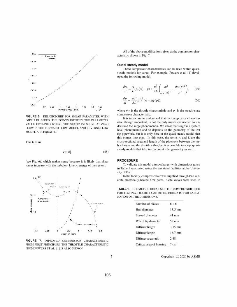
FIGURE 6. RELATIONSHIP FOR SHEAR PARAMETER WITHIMPELLER SPEED. THE POINTS IDENTIFY THE PARAMETERVALUE OBTAINED WHERE THE STATIC PRESSURE AT ZEROFLOW IN THE FORWARD FLOW MODEL AND REVERSE FLOWMODEL ARE EQUATED.
This tells us
ν ∝ u2θ (48)
(see Fig. 6), which makes sense because it is likely that shearlosses increase with the turbulent kinetic energy of the system.
FIGURE 7. IMPROVED COMPRESSOR CHARACTERISTICFROM FIRST PRINCIPLES. THE THROTTLE CHARACTERISTICFROM POWERS ET AL. [1] IS ALSO SHOWN.
All of the above modifications gives us the compressor char-acteristic shown in Fig. 7.
Quasi-steady modelThese compressor characteristics can be used within quasi-
steady models for surge. For example, Powers et al. [1] devel-oped the following model:
dmdt
=AL(pc(m)− p)+
κ1γ
AL
(m2
pc(m)1γ− mT (p)2
p1γ
), (49)
d pdt
=γκ
1γ
ALp
γ−1γ (m− mT (p)), (50)
where mT is the throttle characteristic and pc is the steady-statecompressor characteristic.
It is important to understand that the compressor character-istic, though important, is not the only ingredient needed to un-derstand the surge phenomenon. We know that surge is a systemlevel phenomenon and so depends on the geometry of the testrig pipework, but it is only here in the quasi-steady model thatthis comes into play. In this case, the terms A and L are thecross-sectional area and length of the pipework between the tur-bocharger and the throttle valve, but it is possible to adopt quasi-steady models that take into account inlet geometry as well.
PROCEDURETo validate this model a turbocharger with dimensions given
in Table 1 was tested using the gas stand facilities at the Univer-sity of Bath.
In the facility, compressed air was supplied through two sep-arate electrically heated flow paths. Gate valves were used to
TABLE 1. GEOMETRIC DETAILS OF THE COMPRESSOR USEDFOR TESTING. FIGURE 1 CAN BE REFERRED TO FOR EXPLA-NATION OF THE DIMENSIONS.
Number of blades 6+6
Hub diameter 13.5 mm
Shroud diameter 41 mm
Wheel tip diameter 58 mm
Diffuser height 3.15 mm
Diffuser length 16.7 mm
Diffuser area ratio 2.48
Critical area of housing 7 cm2
7 Copyright c© 2020 by ASME
106

FIGURE 8. SCHEMATIC OF THE GAS STAND USED TO TESTTHE COMPRESSORS.
control the flow. One flow was used to drive the turbine andwas in the conventional direction, entering at the turbine inlet.This was the predominant means of controlling the speed of theturbocharger. The other compressed air stream was fed in the re-verse flow direction through the compressor, entering at the com-pressor outlet. See Fig. 8 for a schematic of the test rig set-up.
To run the experiment, air was let into the turbine side todrive the rotor. The valve feeding air to the compressor outletremained closed so there was no air going through the compres-sor side. This led to surging behaviour with an audible pulsatingflow. The turbine speed was limited to approximately 20,000 rpmso not to cause damage to the compressor.
Compressed air was then fed into the compressor side in thereverse direction by opening the valve. This stopped the surgingbehaviour and stabilised the flow.
The turbine speed was then increased to the desired values.The compressor side valve was adjusted to keep the flow in thestable backflow regime throughout the testing. At fixed speeds,the compressor side mass flow was slowly increased from 15g/sto 80g/s to map out the reversed flow characteristic. This wasrepeated multiple times and for multiple different speeds.
A high-frequency pressure measurement was recorded tocheck the steadiness of the flow. Since the flow was found tobe steady, measurements were taken at 10Hz of the mass flow,temperature and pressure on the compressor side. A V-cone wasused to measure the mass flow, PRTs for the temperature, andpneumatically averaged pressure transducers for static and to-
tal pressure measurements. The locations and accuracy of thesemeasurements are indicated in Fig. 8.
RESULTS AND DISCUSSIONThe first interesting observation was that the flow was surg-
ing when the valve feeding air into the compressor was fullyclosed. A snapshot of this is shown in Fig. 9. Therefore, it ishighly probable that the flow dynamics are continually unsteadybetween zero flow and the surge line in forward flow. Combiningthis with the fact that the flow dynamics at negative mass flowswas observed to be steady, shows us that a switch of stability hasto occur at zero mass flow. Therefore, this supports our new stallfunction with a local minimum at zero flow.
The next important result to recognise is that the flow issteady in the reverse flow region. Consider the Moore-Greitzermodel (Eqns. 1 & 2) [12]:
dΦdt
= B(ψc−Ψ) = f (Φ,Ψ), (51)
dΨdt
=1B(Φ−ψ−1
T ) = g(Φ,Ψ). (52)
Computing the Jacobian, J, allows us to determine regions ofstability for this model:
J =
[d fdΦ
d fdΨ
dgdΦ
dgdΨ
]=
B dψc
dΦ −B1B − 1
B
(dψTdΦ
)−1
. (53)
FIGURE 9. SURGING BEHAVIOUR OF THE COMPRESSORWHEN OPERATING AT ZERO MASS FLOW.
8 Copyright c© 2020 by ASME
107

FIGURE 10. RECORDED COMPRESSOR MAPPINGS IN NEGATIVE MASS FLOW REGION AT DIFFERENT IMPELLER SPEEDS. LEFTSHOWS THE RAW DATA AND THE RIGHT SHOWS A COMPARISON BETWEEN THE DATA AND THE MODEL. THEORETICAL ASYMP-TOTES FOR THE DATA HAVE BEEN ADDED IN GREY TO THE RIGHT HAND PLOT. THE SPEEDS INDICATED ON EACH LINE ARE INKRPM.
The system is stable if detJ > 0 and trJ < 0 [19]. In our case,
detJ = 1− dψc
dΦ
(dψT
dΦ
)−1
, (54)
trJ = Bdψc
dΦ− 1
B
(dψT
dΦ
)−1
. (55)
The surge models in literature all have a throttle characteris-tic with a positive gradient (see Fig. 7). Also, as most models arebased on the cubic characteristic of Moore and Greitzer (Eqn. 4)they tend to assume a negative gradient of the compressor char-acteristic. The model we developed above also has this featureof a negative slope in the reverse flow region.
This means that
dψT
dΦ> 0>
dψc
dΦ(56)
=⇒ dψc
dΦ
(dψT
dΦ
)−1
< 1 (57)
=⇒ detJ > 0 (58)
and
dψT
dΦ> 0,
dψc
dΦ< 0 (59)
=⇒ trJ = Bdψc
dΦ− 1
B
(dψT
dΦ
)−1
< 0 (60)
so having a negative gradient of the compressor characteristic re-sults in a mathematically stable system and hence steady flow. Soobserving experimentally stable flow supports compressor char-acteristics having a negative gradient in the negative mass flowregion.
The left-hand plot of Fig. 10 shows the raw test data obtainedin the pressure-mass flow plane at different impeller speeds. Theright-hand plot shows how this data compares to the model devel-oped in the previous sections. We can see that we achieve a goodquantitative fit to our model for all points, except the near-zeropoints at higher impeller speeds.
The 85krpm and 95krpm speed lines also have a good qual-itative fit because they share the same quadratic-like shape thatour model predicts. Therefore, the model we developed abovemust capture the predominant physics going on in reverse flow.
Looking closely at the raw data, we can see a gradual changein shape of the reverse flow characteristic as the impeller speed
9 Copyright c© 2020 by ASME
108
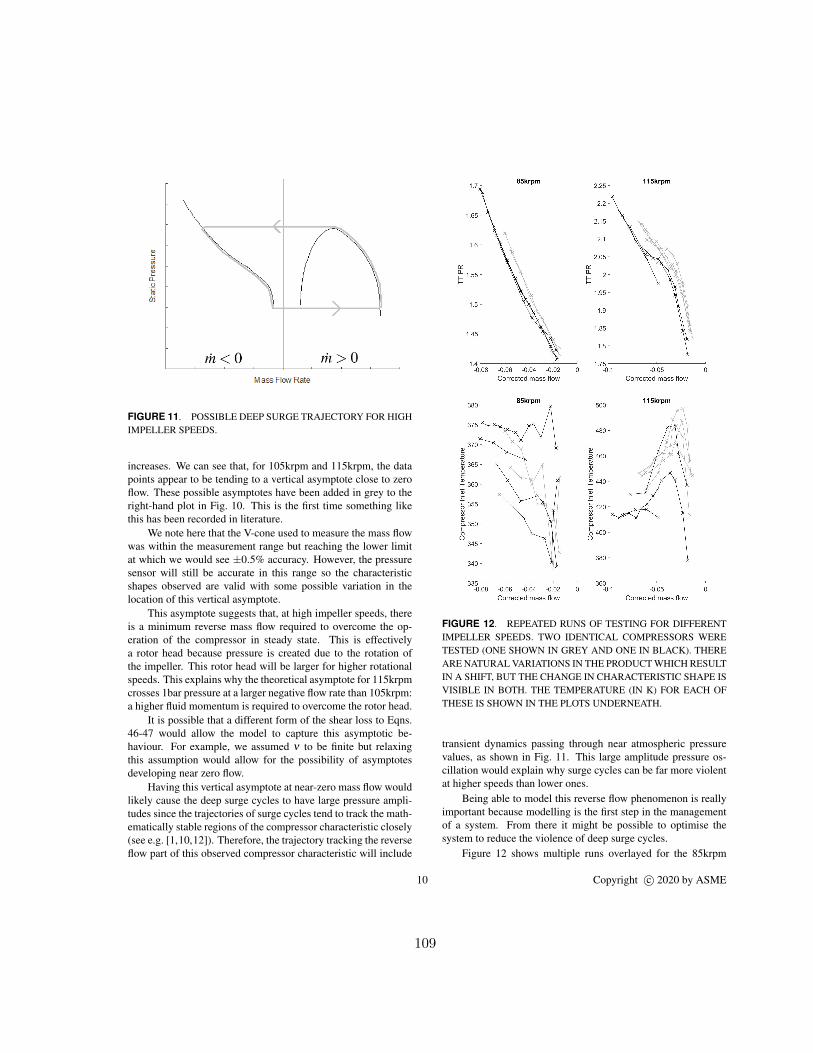
FIGURE 11. POSSIBLE DEEP SURGE TRAJECTORY FOR HIGHIMPELLER SPEEDS.
increases. We can see that, for 105krpm and 115krpm, the datapoints appear to be tending to a vertical asymptote close to zeroflow. These possible asymptotes have been added in grey to theright-hand plot in Fig. 10. This is the first time something likethis has been recorded in literature.
We note here that the V-cone used to measure the mass flowwas within the measurement range but reaching the lower limitat which we would see ±0.5% accuracy. However, the pressuresensor will still be accurate in this range so the characteristicshapes observed are valid with some possible variation in thelocation of this vertical asymptote.
This asymptote suggests that, at high impeller speeds, thereis a minimum reverse mass flow required to overcome the op-eration of the compressor in steady state. This is effectivelya rotor head because pressure is created due to the rotation ofthe impeller. This rotor head will be larger for higher rotationalspeeds. This explains why the theoretical asymptote for 115krpmcrosses 1bar pressure at a larger negative flow rate than 105krpm:a higher fluid momentum is required to overcome the rotor head.
It is possible that a different form of the shear loss to Eqns.46-47 would allow the model to capture this asymptotic be-haviour. For example, we assumed ν to be finite but relaxingthis assumption would allow for the possibility of asymptotesdeveloping near zero flow.
Having this vertical asymptote at near-zero mass flow wouldlikely cause the deep surge cycles to have large pressure ampli-tudes since the trajectories of surge cycles tend to track the math-ematically stable regions of the compressor characteristic closely(see e.g. [1,10,12]). Therefore, the trajectory tracking the reverseflow part of this observed compressor characteristic will include
FIGURE 12. REPEATED RUNS OF TESTING FOR DIFFERENTIMPELLER SPEEDS. TWO IDENTICAL COMPRESSORS WERETESTED (ONE SHOWN IN GREY AND ONE IN BLACK). THEREARE NATURAL VARIATIONS IN THE PRODUCT WHICH RESULTIN A SHIFT, BUT THE CHANGE IN CHARACTERISTIC SHAPE ISVISIBLE IN BOTH. THE TEMPERATURE (IN K) FOR EACH OFTHESE IS SHOWN IN THE PLOTS UNDERNEATH.
transient dynamics passing through near atmospheric pressurevalues, as shown in Fig. 11. This large amplitude pressure os-cillation would explain why surge cycles can be far more violentat higher speeds than lower ones.
Being able to model this reverse flow phenomenon is reallyimportant because modelling is the first step in the managementof a system. From there it might be possible to optimise thesystem to reduce the violence of deep surge cycles.
Figure 12 shows multiple runs overlayed for the 85krpm
10 Copyright c© 2020 by ASME
109

and 115 krpm speed lines, the temperature at each of these runsis shown below them. These runs were performed on differentdays, with the test cell starting cold and starting warm. For lowimpeller speeds the repeatability was good. However, the vari-ability in the repeats increased with impeller speed.
From looking at the plots of temperature, we believe that thisis not the cause of the variability. There is a large variability inthe temperature of the points at both speeds, but only minimalchange in the repeat runs for 85krpm. If it were the tempera-ture, we would expect to see the variability in both 85krpm and115krpm.
During testing, we noticed that the main cause of variationseemed to be the starting condition. We usually started at lowmass flows and swept gradually upwards to larger ones, but start-ing part way up this sweep gave us different results initially. Thiscould mean that either (i) the system itself is sensitive, or (ii) thetwo types of dynamics creating the change in characteristic shapeare interacting or can be observed at the same mass flow depen-dent on the starting conditions.
It is interesting to note that the highest temperaturesrecorded for 115krpm coincide with the points at which we getthis transition from the quadratic-like shape to the asymptoticbehaviour. Therefore, any physical phenomenon that causes thistransition appears to result in a large rise in temperature.
We tested two identical turbochargers during these reversedflow experiments and we have plotted the results from both onFig. 12. There is standard manufacturing variability betweenthe two turbochargers, but it is interesting to note that both tur-bochargers observed this change in characteristic shape with im-peller speed.
We would have liked to obtain results at higher impellerspeeds. However, pushing the turbine to higher speeds whilemaintaining the reversed flow conditions in the impeller leads tocatastrophic failure of the turbocharger (see Fig. 13). We alsodecided not to test at larger negative mass flows due to the riskof causing a failure, because the temperature of the system wasreaching values over 200oC.
FIGURE 13. TURBOCHARGER FAILURE AS A RESULT OFTESTING AT 135 KRPM.
CONCLUSIONSThe majority of surge models for turbochargers rely on a
steady-state compressor characteristic that is extrapolated intothe reverse flow region. We have conducted experiments to mea-sure the characteristic in the region of negative mass flows. Wehave shown that the flow operates stably in this case, which pro-vides supporting evidence for the models like the Moore-Greiztermodel.
We further developed the model by Powers et al. [1], tak-ing care of the dynamics and boundary conditions that hold inreversed flow conditions. We suggested a new stall function thatresults in a characteristic with a local minimum at zero flow, andhave provided supporting experimental evidence for this.
We experimentally identified a change in characteristicshape as the impeller speed increases. This is the first time sucha change has been recorded, and it suggests that the physical dy-namics of the flow change at high impeller speeds at near-zeroflow.
The model in the reverse flow regime showed excellentagreement to the experimental data. However, the model doesn’tcurrently capture the change in characteristic shape. This phe-nomenon is likely to be caused by a rotor head, and further workis planned to incorporate this into the mathematical model byusing a different form of shear loss at the impeller-diffuser inter-face.
ACKNOWLEDGMENTThe authors very are grateful to Cummins Turbo Technolo-
gies for their continued support of this work and, particularly, forproviding the turbochargers used for carrying out this test work.
Katherine Powers is supported by a scholarship from the EP-SRC Centre for Doctoral Training in Statistical Applied Mathe-matics at Bath (SAMBa), under the project EP/L015684/1.
REFERENCES[1] Powers, K. H., Brace, C. J., Budd, C. J., Copeland, C. D.,
and Milewski, P. A. “Modelling axisymmetric centrifu-gal compressor characteristics from first principles”. InASME Turbo Expo 2019: Turbomachinery Technical Con-ference and Exposition, American Society of MechanicalEngineers Digital Collection.
[2] Watson, N., and Janota, M. S., 1982. Turbocharging: Theinternal combustion engine. MacMillan.
[3] Stone, R., 2012. Introduction to internal combustion en-gines, 4 ed. Palgrave MacMillan.
[4] Emmons, H. W., Pearson, C. E., and Grant, H. P., 1955.“Compressor surge and stall propagation, traks”. ASME.
[5] Fink, D. A., Cumpsty, N. A., and Greitzer, E. M., 1992.“Surge dynamics in a free-spool centrifugal compressorsystem”. Journal of Turbomachinery, 114, pp. 321– 332.
11 Copyright c© 2020 by ASME
110
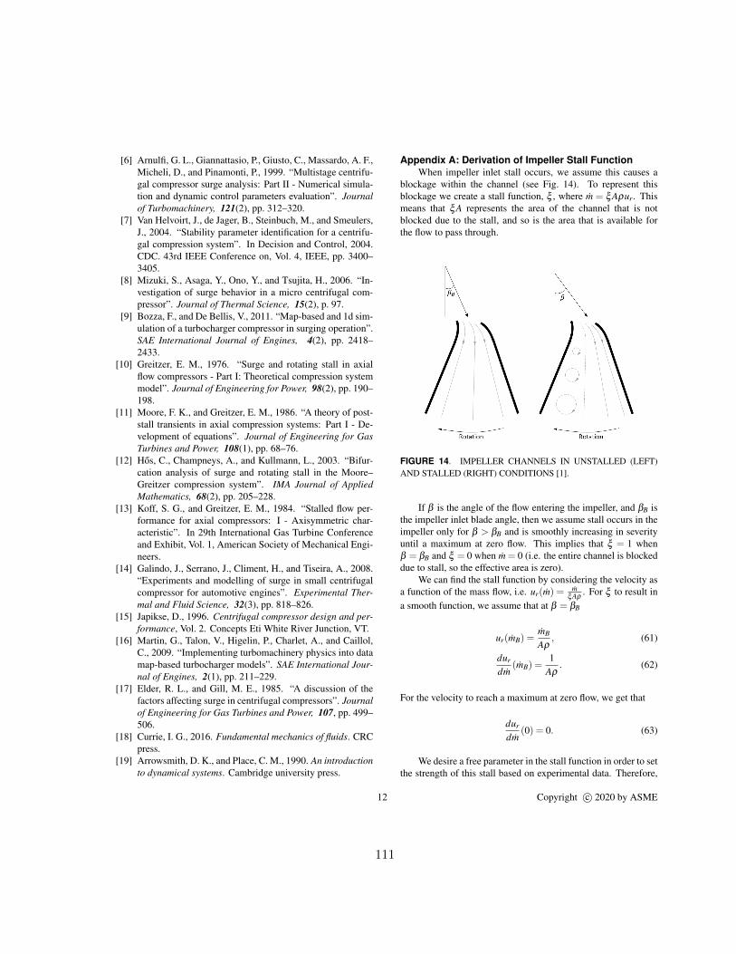
[6] Arnulfi, G. L., Giannattasio, P., Giusto, C., Massardo, A. F.,Micheli, D., and Pinamonti, P., 1999. “Multistage centrifu-gal compressor surge analysis: Part II - Numerical simula-tion and dynamic control parameters evaluation”. Journalof Turbomachinery, 121(2), pp. 312–320.
[7] Van Helvoirt, J., de Jager, B., Steinbuch, M., and Smeulers,J., 2004. “Stability parameter identification for a centrifu-gal compression system”. In Decision and Control, 2004.CDC. 43rd IEEE Conference on, Vol. 4, IEEE, pp. 3400–3405.
[8] Mizuki, S., Asaga, Y., Ono, Y., and Tsujita, H., 2006. “In-vestigation of surge behavior in a micro centrifugal com-pressor”. Journal of Thermal Science, 15(2), p. 97.
[9] Bozza, F., and De Bellis, V., 2011. “Map-based and 1d sim-ulation of a turbocharger compressor in surging operation”.SAE International Journal of Engines, 4(2), pp. 2418–2433.
[10] Greitzer, E. M., 1976. “Surge and rotating stall in axialflow compressors - Part I: Theoretical compression systemmodel”. Journal of Engineering for Power, 98(2), pp. 190–198.
[11] Moore, F. K., and Greitzer, E. M., 1986. “A theory of post-stall transients in axial compression systems: Part I - De-velopment of equations”. Journal of Engineering for GasTurbines and Power, 108(1), pp. 68–76.
[12] Hos, C., Champneys, A., and Kullmann, L., 2003. “Bifur-cation analysis of surge and rotating stall in the Moore–Greitzer compression system”. IMA Journal of AppliedMathematics, 68(2), pp. 205–228.
[13] Koff, S. G., and Greitzer, E. M., 1984. “Stalled flow per-formance for axial compressors: I - Axisymmetric char-acteristic”. In 29th International Gas Turbine Conferenceand Exhibit, Vol. 1, American Society of Mechanical Engi-neers.
[14] Galindo, J., Serrano, J., Climent, H., and Tiseira, A., 2008.“Experiments and modelling of surge in small centrifugalcompressor for automotive engines”. Experimental Ther-mal and Fluid Science, 32(3), pp. 818–826.
[15] Japikse, D., 1996. Centrifugal compressor design and per-formance, Vol. 2. Concepts Eti White River Junction, VT.
[16] Martin, G., Talon, V., Higelin, P., Charlet, A., and Caillol,C., 2009. “Implementing turbomachinery physics into datamap-based turbocharger models”. SAE International Jour-nal of Engines, 2(1), pp. 211–229.
[17] Elder, R. L., and Gill, M. E., 1985. “A discussion of thefactors affecting surge in centrifugal compressors”. Journalof Engineering for Gas Turbines and Power, 107, pp. 499–506.
[18] Currie, I. G., 2016. Fundamental mechanics of fluids. CRCpress.
[19] Arrowsmith, D. K., and Place, C. M., 1990. An introductionto dynamical systems. Cambridge university press.
Appendix A: Derivation of Impeller Stall FunctionWhen impeller inlet stall occurs, we assume this causes a
blockage within the channel (see Fig. 14). To represent thisblockage we create a stall function, ξ , where m = ξ Aρur. Thismeans that ξ A represents the area of the channel that is notblocked due to the stall, and so is the area that is available forthe flow to pass through.
FIGURE 14. IMPELLER CHANNELS IN UNSTALLED (LEFT)AND STALLED (RIGHT) CONDITIONS [1].
If β is the angle of the flow entering the impeller, and βB isthe impeller inlet blade angle, then we assume stall occurs in theimpeller only for β > βB and is smoothly increasing in severityuntil a maximum at zero flow. This implies that ξ = 1 whenβ = βB and ξ = 0 when m = 0 (i.e. the entire channel is blockeddue to stall, so the effective area is zero).
We can find the stall function by considering the velocity asa function of the mass flow, i.e. ur(m) = m
ξ Aρ . For ξ to result ina smooth function, we assume that at β = βB
ur(mB) =mB
Aρ, (61)
dur
dm(mB) =
1Aρ
. (62)
For the velocity to reach a maximum at zero flow, we get that
dur
dm(0) = 0. (63)
We desire a free parameter in the stall function in order to setthe strength of this stall based on experimental data. Therefore,
12 Copyright c© 2020 by ASME
111

with three conditions and a free parameter, the simplest functionwe can use to describe the stalled velocity is a cubic:
ur = am3 +bm2 + cm+d. (64)
Differentiating this gives
dur
dm= 3am2 +2bm+ c. (65)
Therefore, Eqn. 63 leads to c = 0 and Eqn. 62 gives us
3am2B +2bmB =
1Aρ
(66)
=⇒ b =1
2AρmB− 3
2amB. (67)
Finally, Eqn. 61 gives us
am3B +
(1
2AρmB− 3
2amB
)m2
B +d =mB
Aρ(68)
=⇒ d =mB
2Aρ+
a2
m3B. (69)
Therefore, the stalled velocity has the form
ur(m) = am3 +(
12AρmB
− 32 amB
)m2 +
(mB2Aρ + a
2 m3B
)(70)
=⇒ mAρξ = am3 +
(1
2AρmB− 3
2 amB
)m2 +
(mB2Aρ + a
2 m3B
)(71)
=⇒ 1ξ = (aAρm2
B)m2
m2B+(
m2mB− 3
2 (aAρm2B)
mmB
)+(
mB2m +
(aAρm2B)
2mBm
). (72)
Let a = aAρm2B, then
1ξ= a
m2
m2B+
(12− 3
2a)
mmB
+
(12+
12
a)
mB
m(73)
=⇒ 1ξ = 1
2
(m
mB+ mB
m
)+ a(1+ 1
2mBm
)( mmB−1)2. (74)
Finally notice that
mmB
=Aρur
AρuBr=
ur
ΩrΩruB
r=
tanβB
tanβ, (75)
so the stall function becomes
ξ =1
12
(tanβBtanβ + tanβ
tanβB
)+ a(
1+ 12
tanβtanβB
)(tanβBtanβ −1
)2 . (76)
13 Copyright c© 2020 by ASME
112
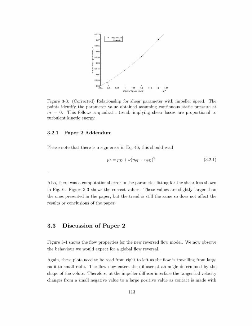
Figure 3-3: (Corrected) Relationship for shear parameter with impeller speed. Thepoints identify the parameter value obtained assuming continuous static pressure atm = 0. This follows a quadratic trend, implying shear losses are proportional toturbulent kinetic energy.
3.2.1 Paper 2 Addendum
Please note that there is a sign error in Eq. 46, this should read
pI = pD + ν(uθI − uθD)2. (3.2.1)
.
Also, there was a computational error in the parameter fitting for the shear loss shown
in Fig. 6. Figure 3-3 shows the correct values. These values are slightly larger than
the ones presented in the paper, but the trend is still the same so does not affect the
results or conclusions of the paper.
3.3 Discussion of Paper 2
Figure 3-4 shows the flow properties for the new reversed flow model. We now observe
the behaviour we would expect for a global flow reversal.
Again, these plots need to be read from right to left as the flow is travelling from large
radii to small radii. The flow now enters the diffuser at an angle determined by the
shape of the volute. Therefore, at the impeller-diffuser interface the tangential velocity
changes from a small negative value to a large positive value as contact is made with
113

Figure 3-4: Properties of flow at a m = −0.02kg/s for the model developed in Section3.2. Black lines denote flow in the impeller and grey lines denote flow in the diffuser.
the impeller blades.
There is also a shear layer that acts instantaneously at the impeller-diffuser interface.
The shear losses produce extra heat, which is why there is a sudden rise in temperature.
There is also a jump in pressure because the flow satisfies the state equation p = ρRT .
One of the interesting things about the reversed flow regime, is that it is stable despite
being an off-design condition with complex flow dynamics.
Figure 3-5 shows our model simulating the experimental reversed flow testing performed
in Paper 2. For a typical surge experiment, the throttle valve would exit into ambient
air, and so the intercept of the throttle curve is approximately 1 bar. However, since we
are feeding compressed air into the compressor outlet, this is equivalent to having a very
high pressure at the outlet of the throttle valve. Therefore, the throttle characteristic
has shifted vertically to account for this.
We can see that this system is stable because the trajectory moves to the operating
point (the intersection between the compressor and throttle characteristic) and stays
there for all time.
In Paper 2, we showed that the mathematical stability of the system depended on the
gradient of the compressor and throttle characteristics. However, the mathematical
114
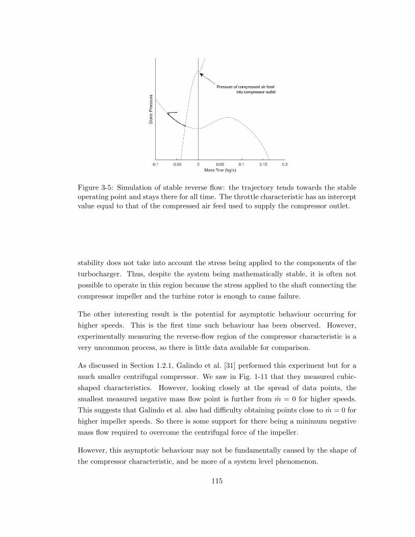
Figure 3-5: Simulation of stable reverse flow: the trajectory tends towards the stableoperating point and stays there for all time. The throttle characteristic has an interceptvalue equal to that of the compressed air feed used to supply the compressor outlet.
stability does not take into account the stress being applied to the components of the
turbocharger. Thus, despite the system being mathematically stable, it is often not
possible to operate in this region because the stress applied to the shaft connecting the
compressor impeller and the turbine rotor is enough to cause failure.
The other interesting result is the potential for asymptotic behaviour occurring for
higher speeds. This is the first time such behaviour has been observed. However,
experimentally measuring the reverse-flow region of the compressor characteristic is a
very uncommon process, so there is little data available for comparison.
As discussed in Section 1.2.1, Galindo et al. [31] performed this experiment but for a
much smaller centrifugal compressor. We saw in Fig. 1-11 that they measured cubic-
shaped characteristics. However, looking closely at the spread of data points, the
smallest measured negative mass flow point is further from m = 0 for higher speeds.
This suggests that Galindo et al. also had difficulty obtaining points close to m = 0 for
higher impeller speeds. So there is some support for there being a minimum negative
mass flow required to overcome the centrifugal force of the impeller.
However, this asymptotic behaviour may not be fundamentally caused by the shape of
the compressor characteristic, and be more of a system level phenomenon.
115
3.4 Conclusions
In this chapter we have derived a model for flow travelling in the reverse direction
through a centrifugal compressor. We recognised that the model in Section 2.5 treated
flow reversal in a way that is similar to local flow recirculation, but we were after the
properties of the compressor for when global flow reversal occurred.
We created a new boundary condition for tangential velocity, based on the geometry
of the volute. We also incorporated a shear layer at the impeller-diffuser interface.
We combined this new reverse flow model with the forward flow model from Section
2.5 using the new form of stall function developed in Section 2.6.1. This has resulted
in a cubic-shaped compressor characteristic with a local minimum at zero flow. This
characteristic is very similar in shape to those commonly used in literature (see Section
1.2.1) but has the advantage of being made from first-principles.
We also discovered possible asymptotic behaviour in the negative flow regime while
undertaking experimental work. This could mean the compressor characteristic itself
should contain an asymptote, or that there is some system level phenomenon that
changes the behaviour of simulations for low mass flows.
The assumption that our compressor characteristic is continuous at zero flow is actively
included in the model developed in Section 3.2 via the choice of the shear loss parameter
ν. Therefore, it is possible to develop a model for the compressor with a different
assumption, which would allow asymptotes to occur.
However, having a continuous curve means we do not have to deal with discontinuous
ODEs while simulating surge. Furthermore, the majority of centrifugal compressor
characteristics proposed in literature are smooth. Therefore, for the next chapter, we
will continue to use this assumption.
116

Chapter 4
Surge Model with Quintic-shaped
Compressor Characteristics and
Spatial Effects
As discussed in Section 2.5, we believe that including diffuser recirculation into the
model for the compressor characteristic may improve the prediction of the surge limit
for higher impeller speeds. Hence, the main focus of this chapter is on including this into
our reduced surge model, and evaluating its performance in comparison to experimental
data.
In order to get a realistic comparison to experimental data, we need to model the
experimental test rig in space and time so we can simulate the behaviour of mass flow
and pressure at locations equivalent to the sensor locations. Therefore, this will require
us to solve a Partial Differential Equation (PDE) system.
117
4.1 PDE Form of the Reduced Surge Model
Recall that, in Section 2.2, we derived two PDEs (Eqs. 2.2.38 and 2.2.39) that simulated
the mass flow and pressure of any constant-area, frictionless pipe. These were
∂p
∂t= −γκ
1γ
Apγ−1γ∂m
∂x, (4.1.1)
∂m
∂t= −A∂p
∂x− κ
1γ
A
∂
∂x
(m2
p1γ
). (4.1.2)
One way to solve these PDEs is by the Method of Lines (see for example [59]), where
a discretisation to the x variable is applied. This results in a system of ODEs for mass
flow and pressure at every point in the spacial discretisation. These ODEs can then be
solved numerically as before using Runga-Kutta methods.
Suppose we have a regular grid of K points in the x direction, with grid spacing ∆x.
Applying a centred difference discretisation to our PDEs results in
∂pj∂t
=γκ
1γ
Apγ−1γ
j
mj−1 − mj+1
2∆x, (4.1.3)
∂mj
∂t= A
pj−1 − pj+1
2∆x+κ
1γ
A
1
2∆x
m
2j−1
p1γ
j−1
−m2j+1
p1γ
j+1
, (4.1.4)
for j = 2, ...,K − 1. To compute∂mj∂t and
∂pj∂t at j = 1 and j = K we would use first
order differences, for example,
∂p1
∂t=γκ
1γ
Apγ−1γ
1
m1 − m2
∆x, (4.1.5)
so we do not require values from outside the domain.
Notice that Eq. 4.1.3 states that p only depends on the neighbouring grid points through
m. Similarly, Eq. 4.1.4 states that the linear contribution to m depends on p only at its
neighbours. Therefore, it makes sense to set up a staggered grid to numerically solve
these PDEs.
Suppose K is even, and we have boundary conditions for p1 and mK . Then solving
on a staggered grid would work by solving Eq. 4.1.3 for p on j = 2, 4, ...,K and Eq.
4.1.4 for m on j = 1, 3, ...,K − 1. To be able to compute Eq. 4.1.4, the values of m on
j = 2, 4, ...,K − 2 are found by linearly interpolating the neighbouring points.
118

Figure 4-1: Model set up for simulating surge behaviour. Both the inlet and outletpipes are modelled using the specified boundary conditions. The numerical solution iscomputed on a staggered grid: white points indicate locations where the pressure PDEis solved and grey points indicate where the mass flow PDE is solved.
The specification of boundary conditions informs us of whether we require K to be
odd or even, and which of Eq. 4.1.3 or 4.1.4 are solved on the even or odd grid points.
Table 4.1 summaries this.
Figure 4-1 shows a simple schematic of the test facility we used to experimentally record
surge behaviour. Measurements we taken at locations both in the inlet pipe and outlet
pipe to the compressor, so we need to model both pipes.
Suppose the inlet pipe is from j = 1, ..,M and the outlet pipe is from j = M + 1, ..., N .
In the test facility, the inlet pipe was open to the room, and so we can set the boundary
condition as p1 = pamb. We also know that the compressor sits between M and M + 1,
meaning that
pM+1 = pc(mM+1, pM ), (4.1.6)
where pc is the steady-state compressor characteristic. We could use this expression to
set a constraint on either pM+1, pM or mM+1.
Boundary conditions K Eq. 4.1.3 Eq. 4.1.4
p1 and mK Even j = 2, 4, ...,K j = 1, 3, ...,K − 1p1 and pK Odd j = 2, 4, ...,K − 1 j = 1, 3, ...,Km1 and pK Even j = 1, 3, ...,K − 1 j = 2, 4, ...,Km1 and mK Odd j = 1, 3, ...,K j = 2, 4, ...,K − 1
Table 4.1: Requirements on number of points, K, in the discretisation, as well as whichequations are solved on which grid points, for each possible pair of boundary conditions.
119

Notice that, if we picked an arbitrary pM+1 (for a given pM ), we could identify multiple
mM that would result in this pressure. Therefore, it is best that we do not invert this
function, and so use this condition to set pM+1.
Furthermore, to allow the compressor to operate freely, we wish to keep mM+1 and pM
as free variables so the boundary condition we specify at M has to be a restriction on
mM . We know that a compressor operating in steady-state has a constant mass flow
across it. Therefore, we can set mM = mM+1.
Finally, at N , we have the throttle and so
mN = mT (pN ) (4.1.7)
holds. The throttle characteristic is a bijection (i.e. each mass flow maps to a unique
pressure and vice versa), and so it does not matter whether this boundary condition is
used to constrain mass flow or pressure.
Referring to Tab. 4.1, these boundary conditions require Eq. 4.1.3 (Eq. 4.1.4) to be
solved on even (resp. odd) grid points for both pipes. We also have the requirement
that M is even, but N can be any integer due to the flexibility of condition 4.1.7.
Another advantage of using a staggered grid is that this system can be related to
previously mentioned ODE systems. Suppose we do not have the inlet pipe, so M = 0
and pM = pamb. Then if we set N = 3, ∆x = 12L2 we get
∂m1
∂t=
2A
L2(pc(m1)− p2) +
2κ1γ
AL2
m2
1
pc(m1)1γ
− (m1 + m3)2
4p1γ
2
, (4.1.8)
∂p2
∂t=γκ
1γ
AL2pγ−1γ
2 (m1 − m3), (4.1.9)
∂m3
∂t=
2A
L2(p2 − pT (m3)) +
2κ1γ
AL2
(m1 + m3)2
4p1γ
2
− m23
pT (m3)1γ
, (4.1.10)
which are equivalent to the ODEs in Greitzer’s 1976 paper [17], once the nonlinearity
120
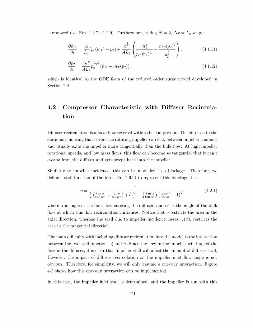
is removed (see Eqs. 1.2.7 - 1.2.9). Furthermore, taking N = 2, ∆x = L2 we get
∂m1
∂t=
A
L2(pc(m1)− p2) +
κ1γ
AL2
m2
1
pc(m1)1γ
− mT (p2)2
p1γ
2
, (4.1.11)
∂p2
∂t=γκ
1γ
AL2pγ−1γ
2 (m1 − mT (p2)). (4.1.12)
which is identical to the ODE form of the reduced order surge model developed in
Section 2.2.
4.2 Compressor Characteristic with Diffuser Recircula-
tion
Diffuser recirculation is a local flow reversal within the compressor. The air close to the
stationary housing that covers the rotating impeller can leak between impeller channels
and usually exits the impeller more tangentially than the bulk flow. At high impeller
rotational speeds, and low mass flows, this flow can become so tangential that it can’t
escape from the diffuser and gets swept back into the impeller.
Similarly to impeller incidence, this can be modelled as a blockage. Therefore, we
define a stall function of the form (Eq. 2.6.9) to represent this blockage, i.e.
η =1
12
(tanαtanα∗ + tanα
tanα∗)
+ b(1 + 1
2tanαtanα∗
) (tanα∗tanα − 1
)2 , (4.2.1)
where α is angle of the bulk flow entering the diffuser, and α∗ is the angle of the bulk
flow at which this flow recirculation initialises. Notice that η restricts the area in the
axial direction, whereas the stall due to impeller incidence losses, ξ(β), restricts the
area in the tangential direction.
The main difficulty with including diffuser recirculation into the model is the interaction
between the two stall functions, ξ and η. Since the flow in the impeller will impact the
flow in the diffuser, it is clear that impeller stall will affect the amount of diffuser stall.
However, the impact of diffuser recirculation on the impeller inlet flow angle is not
obvious. Therefore, for simplicity, we will only assume a one-way interaction. Figure
4-2 shows how this one-way interaction can be implemented.
In this case, the impeller inlet stall is determined, and the impeller is run with this
121

Figure 4-2: Flow chart showing how both impeller inlet stall and diffuser stall areimplemented in the steady-state model for the compressor. Impeller incidence has theability to affect diffuser recirculation, but not vice versa. Subscript 0 denotes an initialvalue.
stalled area to determine the flow angle into the diffuser. The diffuser stall is then
determined and the stalled area recomputed to account for this. The entire system
(both impeller and diffuser) are then run with this stalled area As to simulate the
dynamics.
It is possible to allow the diffuser stall to impact the impeller inlet angle and iteratively
solve to find the stalled area, but this would add extra complexity and computation
time.
The paper in the next section presents the resulting compressor characteristics once
diffuser recirculation is incorporated into the model. It considers how to define the
critical angle α∗, and the stall factor b. It also extends the compressor model to
include some effects of the volute in order to improve the choked-flow properties.
Finally, the paper looks at simulated dynamics of the entire compression system when
this characteristic is incorporated into the PDE model above, and compares these to
experimental data.
122

This declaration concerns the article entitled:
A New First-Principles Model to Predict Incipient and Deep Surge for a Centrifugal Compressor
Publication status (tick one)
Draft manuscript Submitted X In review Accepted Published
Publication details (reference)
Powers, K., Kennedy, I., Archer, J., Eynon, P., Horsley, J., Brace, C., Copeland, C., and Milewski, P. (2021) “A New First-Principles Model to Predict Incipient and Deep Surge for a Centrifugal Compressor.” Journal of Energy (Submitted)
Copyright status (tick the appropriate statement)
I hold the copyright for this material X Copyright is retained by the publisher, but I have
been given permission to replicate the material here
Candidate’s contribution to the paper (provide details, and also indicate as a percentage)
The contribution of Katherine Powers to the paper is as follows:
• Formulation of ideas (90%) with advice from supervising authors
• Derivation of equations for the mathematical models (90%)
• Participation in design and implementation of experiments (40%)
• Writing MATLAB code and creating of numerical simulations (100%)
• Comparing numerical simulations to given experimental data, and analysing of the results (100%)
• Presentation of data in journal format (100%)
Statement from Candidate
This paper reports on original research I conducted during the period of my Higher Degree by Research candidature.
Signed
Date
26/02/2021
4.3 Paper 3: A New First-principles Model to Predict In-
cipient and Deep Surge for a Centrifugal Compressor
123
A New First-principles Model to Predict Incipient and
Deep Surge for a Centrifugal Compressor
Katherine Powersa,1, Ian Kennedyb, Jamie Archerc, Paul Eynonc, JohnHorsleyc, Chris Braceb, Colin Copelandd, Paul Milewskia
aDepartment of Mathematical Sciences, University of Bath, Claverton Down, Bath, BA27AY, UK
bDepartment of Mechanical Engineering, University of Bath, ClavertonDown, Bath, BA2 7AY, UK
cCummins Turbo Technologies, St Andrew’s Road, Huddersfield, HD1 6RA, UKdSchool of Sustainable Energy Engineering, Simon Fraser University, 5118 - 10285
University Drive, Surrey, V3T 0N1, BC, Canada
Abstract
Centrifugal compressors are used in many applications, including micro-gasturbines, automotive turbochargers, and air-conditioning. Compressor surgeis an instability that occurs at low flow rates that is often damaging to thecompressor and its installation. In particular, the incipient surge regime isknown to produce noise characteristics that cause problems with customeracceptance. It is therefore important to be able to predict both incipientand deep surge onset which has historically only been possible to assessexperimentally.
Powers et al. [1, 2] have developed a model for the compressor charac-teristic from first-principles so that surge could be predicted without thereliance on costly testing. In this paper, we will extend their work to includediffuser recirculation and show a new quintic-like shape for the compressorcharacteristic that is able to differentiate between incipient and deep surge.
We will then use this model to simulate the surge behaviour observed ona test rig. We develop a model that allows variations in both space and timeto capture the wave dynamics in the pipework. We explore how the systemevolves from stable operation, through incipient surge, into deep surge. Thismodel is validated via experiment conducted at the University of Bath.
1Please address all correspondence to this author. Email: [email protected]
Preprint submitted to Elsevier 24th February 2021
124
The potential of this model to predict both surge regimes will allow en-gineers to better design centrifugal compressors, and match them to partic-ular applications to avoid problematic surge behaviour, in advance of exper-imental tests.
Keywords: Surge, Centrifugal/Radial Compressors, Compressible Fluids,Reduced order modelling, Ordinary Differential Equations
Nomenclature
A Cross-sectional areaa Impeller inlet stall parameterB Greitzer’s parameterb Diffuser stall parameterc Speed of soundE Specific energyF Friction functionf Friction coefficientfq Frequencyg Acceleration due to gravityh Channel heightL Lengthm Mass flowˆm Effective mass flownb Number of impeller bladesODE Ordinary differential equationp Pressureq Mass flow per radianQ Heat fluxR Specific gas constantr RadiusS Surface area per unit volumes Distance
t TimeT Temperatureu Velocityx Distanceα Wheel exit flow angleα∗ Critical wheel exit flow angleαB Impeller backsweep angleβ Impeller inlet flow angleβB Impeller inlet blade angleγ Specific heat ratio∆x Grid spacingη Diffuser stall functionκ Isentropic constantλ Throttle settingν Shear loss parameterξ Impeller inlet stall functionξT Throttle parametersρ Densityτ Deviatoric stress tensorΦ Nondimensional mass flowΨ Nondimensional pressureΩ Angular rotation
2
125
Subscripts/superscripts:
amb Ambientc CompressorD DiffuserI Impellerr Radial direction
T Throttletip Impeller wheel tipV Voluteθ Tangential direction∗ Critical
1. Introduction
Centrifugal compressors have wide range of applications because com-pressed air is such an important commodity. Compressed air is an importantmedium for energy transfer in many processes, from pneumatics, to vehiclepropulsion and breaks, to refrigeration. In this paper, we will discuss thecentrifugal compressor in the context of automotive turbochargers, but themethodology presented is applicable to many more uses.
Nowadays most road vehicles have downsized turbocharged engines. Thereis a drive to reduce pollutants, especially greenhouse gasses, and downsizedengines are more environmentally friendly [3]. It is the turbocharger thatallows us to use downsized engines because they increase the power outputof that engine making it comparable to the previously used larger naturallyaspirated engines [4].
Surge is an aerodynamic instability that exists when operating the tur-bocharger compressor at low mass flows [4]. Therefore, surge limits the com-pressor operating regime and hence limits the amount of boost provided atlow engine speeds. As a result, being able to predict the onset of surge isvital for engine manufacturers.
Surge causes oscillations in mass flow and pressure. There are differentclasses of surge. When the oscillations in mass flow are large enough that ac-tual flow reversal is seen, this is called deep surge [5]. Operating in deep surgeoften causes damage to the impeller blades within the compressor becausethe oscillations unbalance the machinery and results in contact between theblades and the housing. The temperature rises significantly as a result of os-cillating flow and can sometimes causes connections between the compressorand its installation to fail.
However, when mass flow and pressure oscillations are observed but theflow always remains travelling in the forward direction, this is classed asincipient surge [5]. This form of surge is less damaging, but is still very
3
126
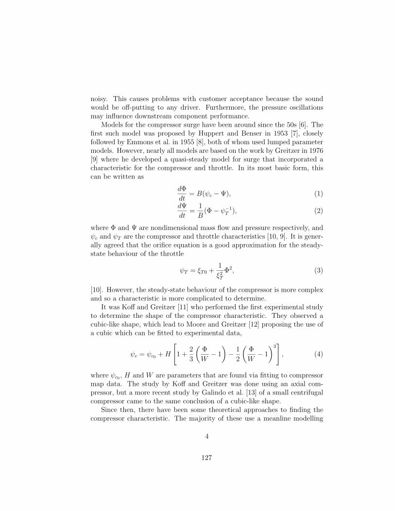
noisy. This causes problems with customer acceptance because the soundwould be off-putting to any driver. Furthermore, the pressure oscillationsmay influence downstream component performance.
Models for the compressor surge have been around since the 50s [6]. Thefirst such model was proposed by Huppert and Benser in 1953 [7], closelyfollowed by Emmons et al. in 1955 [8], both of whom used lumped parametermodels. However, nearly all models are based on the work by Greitzer in 1976[9] where he developed a quasi-steady model for surge that incorporated acharacteristic for the compressor and throttle. In its most basic form, thiscan be written as
dΦ
dt= B(ψc −Ψ), (1)
dΨ
dt=
1
B(Φ− ψ−1T ), (2)
where Φ and Ψ are nondimensional mass flow and pressure respectively, andψc and ψT are the compressor and throttle characteristics [10, 9]. It is gener-ally agreed that the orifice equation is a good approximation for the steady-state behaviour of the throttle
ψT = ξT0 +1
ξ2TΦ2, (3)
[10]. However, the steady-state behaviour of the compressor is more complexand so a characteristic is more complicated to determine.
It was Koff and Greitzer [11] who performed the first experimental studyto determine the shape of the compressor characteristic. They observed acubic-like shape, which lead to Moore and Greitzer [12] proposing the use ofa cubic which can be fitted to experimental data,
ψc = ψc0 +H
[1 +
2
3
(Φ
W− 1
)− 1
2
(Φ
W− 1
)3], (4)
where ψc0 , H and W are parameters that are found via fitting to compressormap data. The study by Koff and Greitzer was done using an axial com-pressor, but a more recent study by Galindo et al. [13] of a small centrifugalcompressor came to the same conclusion of a cubic-like shape.
Since then, there have been some theoretical approaches to finding thecompressor characteristic. The majority of these use a meanline modelling
4
127
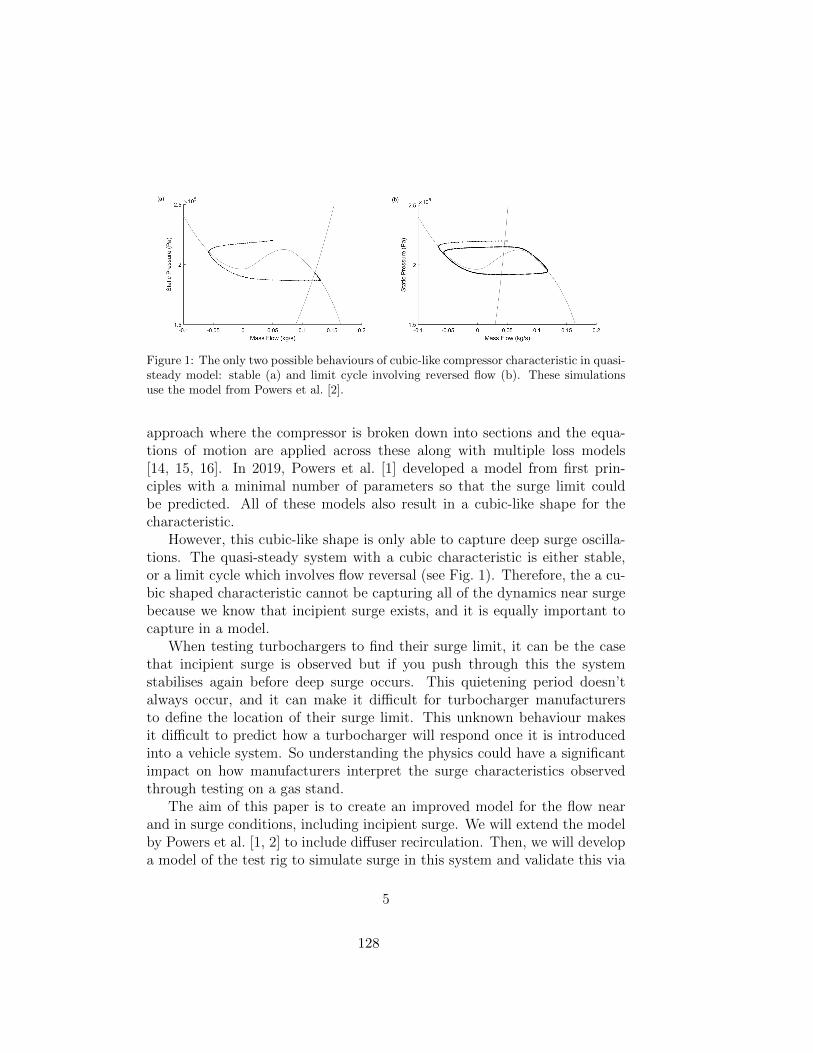
Figure 1: The only two possible behaviours of cubic-like compressor characteristic in quasi-steady model: stable (a) and limit cycle involving reversed flow (b). These simulationsuse the model from Powers et al. [2].
approach where the compressor is broken down into sections and the equa-tions of motion are applied across these along with multiple loss models[14, 15, 16]. In 2019, Powers et al. [1] developed a model from first prin-ciples with a minimal number of parameters so that the surge limit couldbe predicted. All of these models also result in a cubic-like shape for thecharacteristic.
However, this cubic-like shape is only able to capture deep surge oscilla-tions. The quasi-steady system with a cubic characteristic is either stable,or a limit cycle which involves flow reversal (see Fig. 1). Therefore, the a cu-bic shaped characteristic cannot be capturing all of the dynamics near surgebecause we know that incipient surge exists, and it is equally important tocapture in a model.
When testing turbochargers to find their surge limit, it can be the casethat incipient surge is observed but if you push through this the systemstabilises again before deep surge occurs. This quietening period doesn’talways occur, and it can make it difficult for turbocharger manufacturersto define the location of their surge limit. This unknown behaviour makesit difficult to predict how a turbocharger will respond once it is introducedinto a vehicle system. So understanding the physics could have a significantimpact on how manufacturers interpret the surge characteristics observedthrough testing on a gas stand.
The aim of this paper is to create an improved model for the flow nearand in surge conditions, including incipient surge. We will extend the modelby Powers et al. [1, 2] to include diffuser recirculation. Then, we will developa model of the test rig to simulate surge in this system and validate this via
5
128
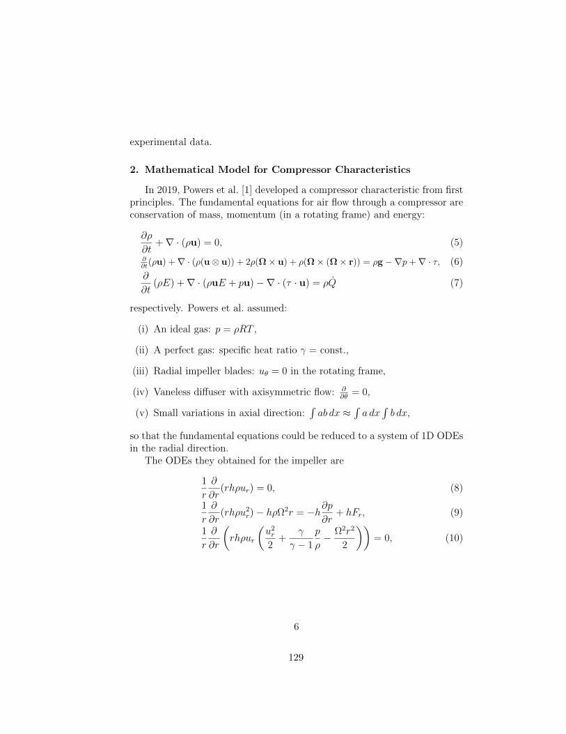
experimental data.
2. Mathematical Model for Compressor Characteristics
In 2019, Powers et al. [1] developed a compressor characteristic from firstprinciples. The fundamental equations for air flow through a compressor areconservation of mass, momentum (in a rotating frame) and energy:
∂ρ
∂t+∇ · (ρu) = 0, (5)
∂∂t
(ρu) +∇ · (ρ(u⊗ u)) + 2ρ(Ω× u) + ρ(Ω× (Ω× r)) = ρg −∇p+∇ · τ, (6)
∂
∂t(ρE) +∇ · (ρuE + pu)−∇ · (τ · u) = ρQ (7)
respectively. Powers et al. assumed:
(i) An ideal gas: p = ρRT ,
(ii) A perfect gas: specific heat ratio γ = const.,
(iii) Radial impeller blades: uθ = 0 in the rotating frame,
(iv) Vaneless diffuser with axisymmetric flow: ∂∂θ
= 0,
(v) Small variations in axial direction:∫ab dx ≈
∫a dx
∫b dx,
so that the fundamental equations could be reduced to a system of 1D ODEsin the radial direction.
The ODEs they obtained for the impeller are
1
r
∂
∂r(rhρur) = 0, (8)
1
r
∂
∂r(rhρu2r)− hρΩ2r = −h∂p
∂r+ hFr, (9)
1
r
∂
∂r
(rhρur
(u2r2
+γ
γ − 1
p
ρ− Ω2r2
2
))= 0, (10)
6
129

and for the diffuser are
1
r
∂
∂r(rhρur) = 0, (11)
1
r
∂
∂r(rhρu2r)−
hρu2θr
= −h∂p∂r
+ hFr, (12)
1
r
∂
∂r(rhρuruθ) +
hρuruθr
= hFθ, (13)
1
r
∂
∂r
(rhρur
(u2r2
+u2θ2
+γ
γ − 1
p
ρ
))= 0, (14)
where
Fr =f
2ρu2rS (15)
Fθ =f
2ρuruθS (16)
represents skin friction.In 2020, Powers et al. [2] developed this further. They suggested a stall
function of
ξ =1
12
(tanβBtanβ
+ tanβtanβB
)+ a
(1 + 1
2tanβtanβB
)(tanβBtanβ
− 1)2 , (17)
to take into account incidence losses. This works by writing m = ξAρur sothat ξA represents the area of the impeller channel that is not blocked dueto stall (see Fig. 2). Therefore, when the flow angle β is equal to the bladeangle βB, ξ = 1 and there is no stalling. However, as β → 90o, ξ → 0 andthe channel becomes fully stalled.
The authors also looked in depth at the reverse flow part of this charac-teristic. In this case, air is travelling from the volute through to the impellerinlet but the impeller wheel is still rotating in the forward direction as thisis controlled by the turbine. In this case, the angle at which air enters fromthe volute into the diffuser has to be specified, and Powers et al. [2] arguedthat this should be
θ = tan−1(uθDurD
)= tan−1
√(
ADA∗
)2
− 1
(18)
7
130

Figure 2: Flow dynamics in an impeller channel with blade angle βB . Left: The flowenters at angle β = βB , and the channel has no stall. Right: The flow enters at angleβ > βB and we have stall that effectively blocks the channel. The flow can only travelthrough an area of ξA.
from geometry considerations. Here, AD = 2πrh is the cross-sectional areaof the diffuser and A∗ is the critical area of the housing.
Another important addition for the reverse flow case is the existence of ashear layer between the diffuser and the impeller. When the air comes intocontact with the impeller it is suddenly accelerated in the opposite direction,and so there is a large change in tangential velocity in a short radial distance.The shear layer causes a loss in pressure due to viscous dissipation. Powerset al. [2] decided to use an instantaneous loss at the interface,
pI = pD + ν(uθI − uθD)2, (19)
where the shear loss parameter ν was found by assuming the characteristicis continuous at zero flow.
8
131
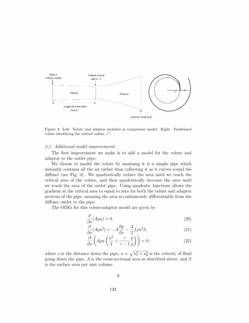
Figure 3: Left: Volute and adaptor included in compressor model. Right: Traditionalvolute identifying the critical radius, r∗.
2.1. Additional model improvements
The first improvement we make is to add a model for the volute andadaptor to the outlet pipe.
We choose to model the volute by assuming it is a simple pipe whichinstantly contains all the air rather than collecting it as it curves round thediffuser (see Fig. 3). We quadratically reduce the area until we reach thecritical area of the volute, and then quadratically increase the area untilwe reach the area of the outlet pipe. Using quadratic functions allows thegradient at the critical area to equal to zero for both the volute and adaptorsections of the pipe, meaning the area is continuously differentiable from thediffuser outlet to the pipe.
The ODEs for this volute-adaptor model are given by
∂
∂s(Aρu) = 0, (20)
∂
∂s(Aρu2) = −A∂p
∂s− A
2fρu2S, (21)
∂
∂s
(Aρu
(u2
2+
γ
γ − 1
p
ρ
))= 0, (22)
where s is the distance down the pipe, u =√u2r + u2θ is the velocity of fluid
going down the pipe, A is the cross-sectional area as described above, and Sis the surface area per unit volume.
9
132

The crucial part of this addition is that it allows us to take the criticalarea of the housing into account. This has improved the choke region ofthe compressor characteristic significantly because, in reality, the flow oftenchokes in the housing, especially for high impeller speeds.
Another improvement we made was to capture some of the effects ofbackswept blades into the model. In order to keep the impeller ODEs simpleand efficient to solve, we wish to keep the assumption of radial blades withinthe impeller. However, we can easily take into account the effect backsweephas on the angle at which the flow exits the impeller into the diffuser by
uθ∣∣tip
= Ωrtip − ur∣∣tip
tan(αB) (23)
where αB is the backsweep angle.Since the flow angle into the diffuser effects how long flow remains in the
diffuser, this addition is able to capture some of the pressure drop backsweptblades cause. It will also allow us the capture how backsweep affects thestability of the system when considering diffuser recirculation in the nextsection.
2.2. Diffuser Recirculation
Diffuser recirculation occurs when air exits the impeller in a predomin-antly tangential direction. When this happens, some of the air does notescape from the diffuser, and instead gets drawn back into the impeller. Dueto leakage flow over the top of the blades, the air exiting the impeller at theshroud-side is usually more tangential than the main flow. Therefore, therecirculation usually occurs here.
This can be accounted for by considering the recirculation as a blockage,in a similar way to the impeller inlet stall developed by Powers et al. [1, 2].This idea is shown in Fig. 4.
In reality, the exit angle of the flow depends on the axial height. There-fore, the critical angle for stall in the diffuser will be the angle at which themain body of the flow has to exit for the shroud-side portion of the flow torecirculate. To get an estimate for this angle, we looked at CFD simulationsfor four different compressors near surge (as this is where diffuser stall islikely to occur). The results are shown in Fig. 5. This shows us that thecritical angle is likely to be in the range of 70o to 75o. In literature, this angleis often given between 75o and 85o [17, 18]. Therefore, we shall use 75o forour critical angle.
10
133

Since we are treating diffuser recirculation as a blockage, we can developa stall function in the exactly same way as Powers et al. [2]. This gives us afunction,
η =1
12
(tanα∗tanα
+ tanαtanα∗
)+ b(1 + 1
2tanαtanα∗
) (tanα∗tanα
− 1)2 , (24)
where α is the flow angle and α∗ is the critical angle. As with impeller inletstall, we have η = 1 implies no stall and η → 0 when the recirculation blocksthe entire channel.
It’s important to notice that, since we have two forms of stalling thateffectively restrict the area inside the compressor, there will be interactionsbetween the two. There is a natural impact of the impeller stall on the diffuserstall because impeller inlet stall will influence the impeller exit velocity, andhence angle α. However, the impact of the diffuser stall on the impeller isnot obvious. Here we assume for simplicity that it doesn’t affect the angleof the incoming flow and so the impeller stall is unaffected by the diffuserstalling.
2.3. Parameter fittings
With these additions to the compressor model, we now have three un-known parameters: (i) f the friction coefficient, (ii) a the stall factor forimpeller inlet stall, and (iii) b the stall factor for diffuser recirculation.
Figure 4: Diffuser stall causing shroud-side recirculation due to air exiting the impellerat an angle greater than a critical angle α > α∗. The recirculation effectively causes ablockage: ηA is the effective area available to the flow.
11
134

Figure 5: CFD data of the average flow angle at the wheel exit close to the surge limit forfour different turbochargers, the tip diameter of which are included in the legend. Eachcompressor was run at five different impeller speeds - the higher speeds correspond to thepoints with higher pressure ratio.
For friction, Powers et al. [1, 2] showed that there existed a linear rela-tionship between the friction factor and the impeller speed. This is because3D losses that are more prominent for higher speeds cannot be captured byour 1D model, and so are being encompassed into the friction factor. For ourmodel, we will use
f = 0.013 + 1.15× 10⁻⁵Ω. (25)
This was found by comparing our model to experimental data for steadypoints.
For impeller inlet stall, Powers et al. [2] showed that a constant stallfactor was able to capture the behaviour. Similarly, in this paper we use aconstant factor of a = 5. This value was calculated by comparing our modelwith the amplitude of deep surge oscillations observed in experiments.
Finally, for diffuser recirculation, we have tuned the stall parameter bycomparing our model with the amplitude of incipient surge oscillations fromexperimental data. See Table 1 for the results. Here, we did not find a re-lationship that can be explained physically, which means that the real-lifesystem is more complex than our model predicts. For example, our assump-tion that the critical angle α∗ is constant with impeller speed and it’s justthe flow angle that changes could be too simplistic. Figure 5 suggests thatthe critical angle could decrease with impeller speed, meaning that stallingoccurs earlier (so b is larger)for higher impeller speeds.
12
135

Figure 6: The variation in the diffuser stall function, η, with stall factor b.
Moreover, the computed values for b only span a small range of the pos-sible values, and they only has a small effect on the stall function. Figure 6shows how the stall function changes with b. It only affects the gradient, i.e.whether stall initially occurs quickly and then slows, or is initially slow andspeeds up.
Universal relations need to be found to make this compressor model fullypredictive. This can be done by regression analysis on a large dataset froma wide range of turbochargers. However, due to a limit of resources availableto the authors, this is out of scope for this paper.
Table 1: Tuned values for diffuser recirculation stall factor b.
Ω b85 krpm 0115 krpm 0.5135 krpm 1.6155 krpm 1.2
13
136

Figure 7: Resulting compressor characteristics when both impeller stall and diffuser recir-culation are included. The impeller speeds in krpm are labelled on each line.
2.4. Resulting characteristic
Similarly to Powers et al. [1, 2], we can reduce the above systems ofequations to the following ODEs:
Impeller:∂ρ
∂r=−ρq2
(1r
+ 1h∂h∂r
)− γΩ2r3h2ρ3 + γfρq2
(nb2πr
+ 1h
)(γ+12
)q2 − (γ − 1)EIr2h2ρ2
, (26)
Diffuser:∂ρ
∂r=−ρq2
r− r2h2ρ3
(γu2θr
+ (γ − 1)uθ∂uθ∂r
)+ γ f
hρq2
(γ+12
)q2 + (γ − 1)
(u2θ2− ED
)r2h2ρ2
, (27)
Volute:∂ρ
∂s=
m2ρfS − 2ρm2 dAds
(3− γ)m2 − 2(γ − 1)EV ρ2A2, (28)
14
137
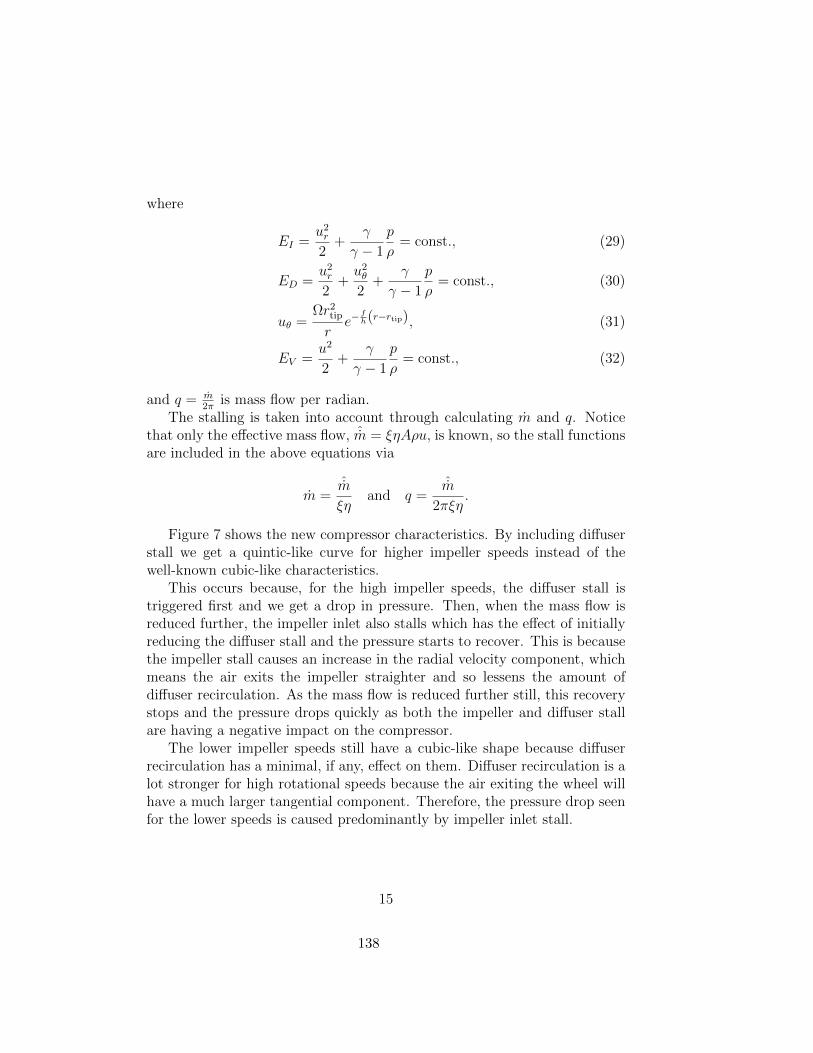
where
EI =u2r2
+γ
γ − 1
p
ρ= const., (29)
ED =u2r2
+u2θ2
+γ
γ − 1
p
ρ= const., (30)
uθ =Ωr2tipr
e−fh(r−rtip), (31)
EV =u2
2+
γ
γ − 1
p
ρ= const., (32)
and q = m2π
is mass flow per radian.The stalling is taken into account through calculating m and q. Notice
that only the effective mass flow, ˆm = ξηAρu, is known, so the stall functionsare included in the above equations via
m =ˆm
ξηand q =
ˆm
2πξη.
Figure 7 shows the new compressor characteristics. By including diffuserstall we get a quintic-like curve for higher impeller speeds instead of thewell-known cubic-like characteristics.
This occurs because, for the high impeller speeds, the diffuser stall istriggered first and we get a drop in pressure. Then, when the mass flow isreduced further, the impeller inlet also stalls which has the effect of initiallyreducing the diffuser stall and the pressure starts to recover. This is becausethe impeller stall causes an increase in the radial velocity component, whichmeans the air exits the impeller straighter and so lessens the amount ofdiffuser recirculation. As the mass flow is reduced further still, this recoverystops and the pressure drops quickly as both the impeller and diffuser stallare having a negative impact on the compressor.
The lower impeller speeds still have a cubic-like shape because diffuserrecirculation has a minimal, if any, effect on them. Diffuser recirculation is alot stronger for high rotational speeds because the air exiting the wheel willhave a much larger tangential component. Therefore, the pressure drop seenfor the lower speeds is caused predominantly by impeller inlet stall.
15
138

Figure 8: Schematic for mathematical test rig model. It is composed of an inlet and outletpipe for the compressor. There is also a throttle valve at the exit of the outlet pipe. Theboundary conditions used for the two pipes are also shown.
3. Mathematical Model for Test Rig
Surge is a system level phenomenon. Therefore, to study this behaviourwe need to model the system around the compressor as well as the compressoritself. Since we will validate this model by comparing it to experimental datagathered on a test rig, we shall create a model consisting of straight inlet andoutlet pipes, with a throttle valve on exit. See Fig. 8 for details.
The fluid in these pipes will obey the standard conservation of mass (Eq.5) and conservation of momentum (Eq. 6) equations. We shall assume that wehave an isentropic flow in the pipes, i.e. p = κργ, to replace the conservationof energy equation. Written in 1D for mass flow and pressure, with directionalong the pipe denoted by x, this gives:
∂p
∂t+γκ
1γ
Apγ−1γ∂m
∂x= 0, (33)
∂m
∂t+ A
∂p
∂x+κ
1γ
A
∂
∂x
(m2
p1γ
)+fSκ
1γ
2A
m2
p1γ
= 0, (34)
where f is a friction factor. Although, f is part of a skin friction term, thisterm will encompass the losses due to dissipation. The flow on exit from thecompressor will be more turbulent than the air prior to it and so we expectthere to be more dissipation losses in the outlet pipe. Therefore, we shall usef = 0.05 in the inlet pipe and f = 0.1 in the outlet pipe.
In order to reduce this to a system of ODEs that can be solved withinMATLAB, we use a centred-difference discretisation in x. Therefore, for a
16
139

location xj within the pipes, and grid spacing ∆x, we have:
∂pj∂t
=γκ
1γ
Apγ−1γ
j
mj−1 − mj+1
2∆x, (35)
∂mj
∂t= A
pj−1 − pj+1
2∆x+κ
1γ
A
1
2∆x
m
2j−1
p1γ
j−1
− m2j+1
p1γ
j+1
− fSκ
1γ
2A
m2j
p1γ
j
. (36)
At each end point of the pipe, we cannot use central differences becauseit would require a point outside of the domain of the pipe. Therefore, we usea first-order difference instead. We also need to specify boundary conditionsfor each end of the pipes. Figure 8 shows the boundary conditions we use.
For the inlet pipe we have a fixed ambient pressure at (1) because thispipe is left open to the room. At (2), we have a constraint that the massflux into the compressor must be the same as that leaving the compressor atpoint (3).
For the outlet pipe, we apply the compressor characteristic developed inSection 2 at (3), which requires both the mass flux through the compressoras well as the inlet pressure to compute the outlet pressure. Finally, we applythe throttle characteristic at (4). We use the same throttle characteristic asPowers et al. [1] but assume constant density for simplicity, namely:
m = sgn(p− pamb)√
2γ
γ − 1ρambA2
λ2
1− λ2 |p− pamb|. (37)
where λ is the fraction the throttle is open, and sgn(x) = x|x| returns the sign
of variable x.
4. Experiments
To provide some validation for this model, we tested a turbocharger usingthe gas stand facilities at the University of Bath. The turbocharger testedhad dimensions given in Table 2, and the layout of the test facility is shownin Fig. 9.
For the turbine section, compressed air was supplied through electricallyheated flow paths and gate valves were used to control the flow. For thecompressor section, the inlet pipe was left open so the compressor could drawair in freely from the test cell room. The amount of flow passing through thecompressor was controlled by a gate valve in the outlet pipe.
17
140

Figure 9: Layout of gas-stand test facility at the University of Bath. The table lists thecomponents with their measurement accuracy where applicable.
To run the experiment, the compressor outlet pipe valve was opened fullyto ensure the turbocharger would initially operate in a non-surge region.
Table 2: Geometric details of the tested compressor.
Number of blades 6 + 6Hub diameter 13.5 mmShroud diameter 41 mmWheel tip diameter 58 mmDiffuser height 3.15 mmDiffuser area ratio 2.48
18
141

Figure 10: (a) Calibration of hotwire sensor to V-cone velocities. A check of the calibrationwas also done with a hot rig. The line where points would lie if the two sensors agreed,along with ±5% error, is shown in grey. (b) Experimental data that contains the highestvelocities (155krpm deep surge operating point) and the calibration limit. A very smallportion of the data lies outside the calibration and so will have lower accuracy. However,this will have minimal impact on the overall result.
Then hot, compressed air was let into the turbine side to drive the rotor.Once the desired rotor speed was reached, the compressor outlet valve wasshut gradually while adjusting the turbine-side valves in order to keep therotor speed constant.
The manufacturer supplied compressor map was used as a guide to identifya near surge location. Starting from this point, high-frequency pressure andflow velocity signals were recorded approximately every 0.002kg/s as the com-pressor outlet valve was closed until the compressor entered deep surge. Thiswas repeated for four different rotor speeds.
A hotwire was used to measure the velocity (and hence, with measured
Figure 11: Grey: Original mass flow data using hotwire sensor. Black: Smoothed signalusing a 100-point moving average.
19
142
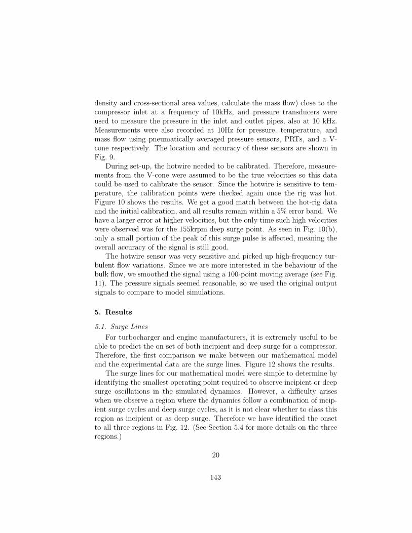
density and cross-sectional area values, calculate the mass flow) close to thecompressor inlet at a frequency of 10kHz, and pressure transducers wereused to measure the pressure in the inlet and outlet pipes, also at 10 kHz.Measurements were also recorded at 10Hz for pressure, temperature, andmass flow using pneumatically averaged pressure sensors, PRTs, and a V-cone respectively. The location and accuracy of these sensors are shown inFig. 9.
During set-up, the hotwire needed to be calibrated. Therefore, measure-ments from the V-cone were assumed to be the true velocities so this datacould be used to calibrate the sensor. Since the hotwire is sensitive to tem-perature, the calibration points were checked again once the rig was hot.Figure 10 shows the results. We get a good match between the hot-rig dataand the initial calibration, and all results remain within a 5% error band. Wehave a larger error at higher velocities, but the only time such high velocitieswere observed was for the 155krpm deep surge point. As seen in Fig. 10(b),only a small portion of the peak of this surge pulse is affected, meaning theoverall accuracy of the signal is still good.
The hotwire sensor was very sensitive and picked up high-frequency tur-bulent flow variations. Since we are more interested in the behaviour of thebulk flow, we smoothed the signal using a 100-point moving average (see Fig.11). The pressure signals seemed reasonable, so we used the original outputsignals to compare to model simulations.
5. Results
5.1. Surge Lines
For turbocharger and engine manufacturers, it is extremely useful to beable to predict the on-set of both incipient and deep surge for a compressor.Therefore, the first comparison we make between our mathematical modeland the experimental data are the surge lines. Figure 12 shows the results.
The surge lines for our mathematical model were simple to determine byidentifying the smallest operating point required to observe incipient or deepsurge oscillations in the simulated dynamics. However, a difficulty ariseswhen we observe a region where the dynamics follow a combination of incip-ient surge cycles and deep surge cycles, as it is not clear whether to class thisregion as incipient or as deep surge. Therefore we have identified the onsetto all three regions in Fig. 12. (See Section 5.4 for more details on the threeregions.)
20
143

Figure 12: A comparison to the model predicted surge lines (black) and the surge lines fromexperimental data (grey). The impeller speeds (in krpm) are labelled on each compressorcharacteristic.
To determine the surge line for the data, we needed to identify the massflow of the operating point, i.e. the average mass flow going through thethrottle. We decided to use the V-cone measurements for this as being furtherfrom the compressor, it shouldn’t be influenced as much by the instantaneousflow dynamics.
For steady operation, the V-cone mass flow gives us the operating point,and for incipient surge, the oscillations are relatively small so the averagemass flow is close to the operating point. However, for deep surge, the massflow oscillations vary a lot and are often far from the operating point. Fur-thermore, the V-cone sensor cannot distinguish between forward and reverseflow as it only identifies the magnitude of the flow, meaning that taking adirect average of this sensor would not be appropriate.
All we know for certain is that the operating point will have a smallermass flow than the previous operating point, and so we chose to use a massflow that was approx. 0.002kg/s smaller than the previous one. For example,for the 155krpm speed line, steady operation was observed for 0.174kg/sthrough to 0.118kg/s. Mild surge was first observed when the flow was re-
21
144

duced further from 0.118kg/s and registered an average flow of 0.106kg/s.Mild surge continued to register through to an average flow of 0.102kg/s.Reducing the flow further resulted in deep surge oscillations which registeredan average flow of 0.109kg/s. Since we know the deep surge was observedafter a reduction in flow from the previous mild surge point, we chose thelocation of the deep surge line to be at a mass flow of 0.1kg/s.
Comparing the incipient surge lines, we see a good match throughout. Wecorrectly predict that there is no incipient surge for the lowest two speeds,and we can predict the onset of incipient surge to within 5% for the top twospeeds.
Notice that the existence of simulated incipient surge dynamics coincideswith quintic-shaped characteristics (not cubic-shaped ones). This impliesthat incipient surge is caused by the interaction of impeller inlet stall anddiffuser recirculation. Since this is the first time a quintic-like characteristichas been captured by any model of a centrifugal compressor, it is the firsttime anyone has suggested a reason for the observed behaviour of incipientsurge.
Looking at the experimental deep surge line, we can see that is it muchcloser to the point at which we simulate a mix of deep and incipient surge,rather than the point at which we simulate full deep surge. This makessense because it is possible for the experimental noise to tip the system fromswitching between incipient and deep surge cycles into solely deep surgecycles, and so this mixed region becomes deep surge.
Moreover, since most compressor mappings are performed in a way toprevent damage occurring, they are likely to back off at the first sign ofdeep surge irrespective of whether this is mixed with incipient oscillations.Therefore, it is likely that most compressor designers would classify thismixed surge region as deep surge because large pressure oscillations occur.
Therefore, assuming the mixed surge region is classified as deep surge, weget a good prediction for the deep surge line as well. We predict deep surgeonset slightly early for low speeds and slightly late for high speeds, but theerror has stayed within 20%.
22
145
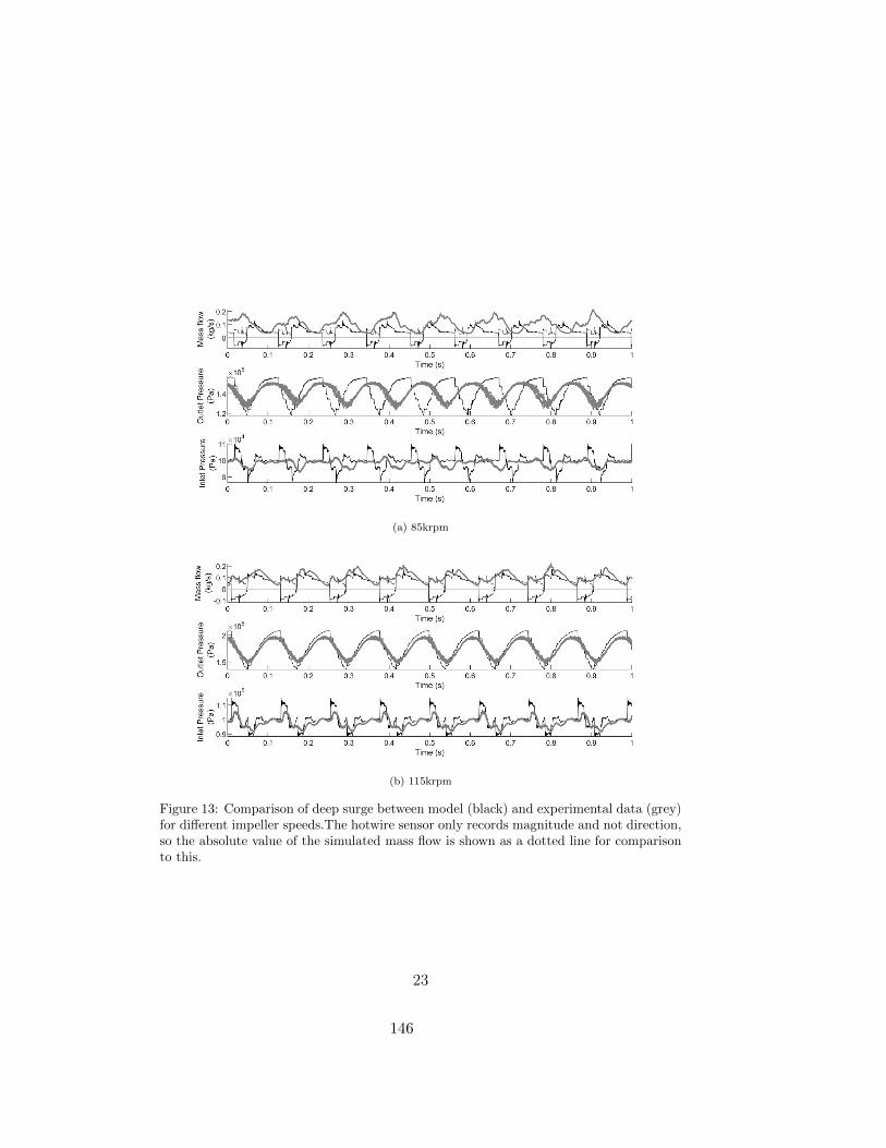
(a) 85krpm
(b) 115krpm
Figure 13: Comparison of deep surge between model (black) and experimental data (grey)for different impeller speeds.The hotwire sensor only records magnitude and not direction,so the absolute value of the simulated mass flow is shown as a dotted line for comparisonto this.
23
146
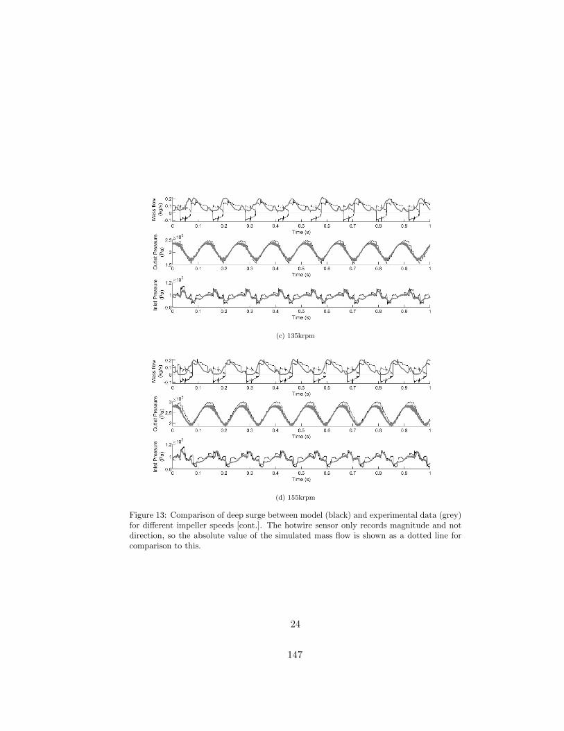
(c) 135krpm
(d) 155krpm
Figure 13: Comparison of deep surge between model (black) and experimental data (grey)for different impeller speeds [cont.]. The hotwire sensor only records magnitude and notdirection, so the absolute value of the simulated mass flow is shown as a dotted line forcomparison to this.
24
147
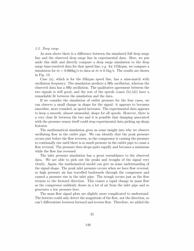
5.2. Deep surge
As seen above there is a difference between the simulated full deep surgeline and the observed deep surge line in experimental data. Here, we putaside this shift and directly compare a deep surge simulation to the deepsurge time-resolved data for that speed line, e.g. for 155krpm, we compare asimulation for m = 0.066kg/s to data at m ≈ 0.1kg/s. The results are shownin Fig. 13.
Case (a), which is for the 85krpm speed line, has a miss-match withoscillation frequency. The simulation predicts a 9Hz oscillation, whereas theobserved data has a 8Hz oscillation. The qualitative agreement between thetwo signals is still good, and the rest of the speeds (cases (b)-(d)) have aremarkable fit between the simulation and the data.
If we consider the simulation of outlet pressure for the four cases, wecan observe a small change in shape for the signal: it appears to becomessmoother, more rounded, as speed increases. The experimental data appearsto keep a smooth, almost sinusoidal, shape for all speeds. However, there isa very close fit between the two and it is possible that damping associatedwith the pressure sensor itself could stop experimental data picking up sharpfeatures.
The mathematical simulation gives us some insight into why we observeoscillating flow in the outlet pipe. We can identify that the peak pressureoccurs just before the flow reverses, so the compressor is causing the pressureto continually rise until there is so much pressure in the outlet pipe to cause aflow reversal. The pressure then drops quite rapidly and becomes a minimumwhile the flow has reversed.
The inlet pressure simulation has a great resemblance to the observeddata. We are able to pick out the peaks and troughs of the signal veryclearly. Again, the mathematical model can give us some understanding ofthe signal shape. The peak inlet pressure occurs when we have flow reversal,so high pressure air has travelled backwards through the compressor andcaused a pressure rise in the inlet pipe. The trough occurs just as the flowreturns to the forward direction. This causes a rapid change in mass flowas the compressor suddenly draws in a lot of air from the inlet pipe and sogenerates a low pressure here.
The mass flow signal plots are slightly more complicated to understand.The hotwire could only detect the magnitude of the flow, not the direction, socan’t differentiate between forward and reverse flow. Therefore, we added the
25
148

plot |m| for the simulated flow as a dotted line in order to compare with thedata collected. Looking at case (b), with impeller speed 115krpm, gives thebest comparison between the simulation and the data. It follows the dottedline very closely, and so the data was able to identify both the forward andreverse flow signals. For all cases, the data and simulation are a good matchfor the forward flow peaks. However, for case (d) the hotwire did not appearto pick up the reverse flow and so shows as near zero during this period.
5.3. Incipient surge
We now do a similar comparison for incipient surge. The results are shownin Fig. 14.
This time, for both cases we have a miss-match of oscillation frequency.The data has an oscillation of approximately 12Hz, whereas our model pre-dicts a frequency of 13Hz instead. This is still very good because we areable to simulate surge behaviour within a frequency of the expected order ofmagnitude.
Overall, the fits are not as good as for the deep surge cases, but our modelis still able to capture a remarkable amount of the features seen in the data.For example, for mass flow, we are able to pick out a signal with the correctamplitude and even pick out the double-peak or trough that is observed inthe data.
For the outlet pressure, our simulation has a higher average pressure anda slightly larger amplitude than observed in the data. However, the shape ofthe signal is very triangular which agrees with the shape of the data signal.
Finally, for the inlet pressure, our model seems to be predicting a higherpeak inlet pressure for both signals and, as with the outlet pressure, seemsto have a higher average pressure. However, we are still able to capture asignificant amount of the signal shape, especially for case (b).
26
149

(a) 135krpm
(b) 155krpm
Figure 14: Comparison of incipient surge between model (black) and experimental data(grey) for different impeller speeds.
27
150
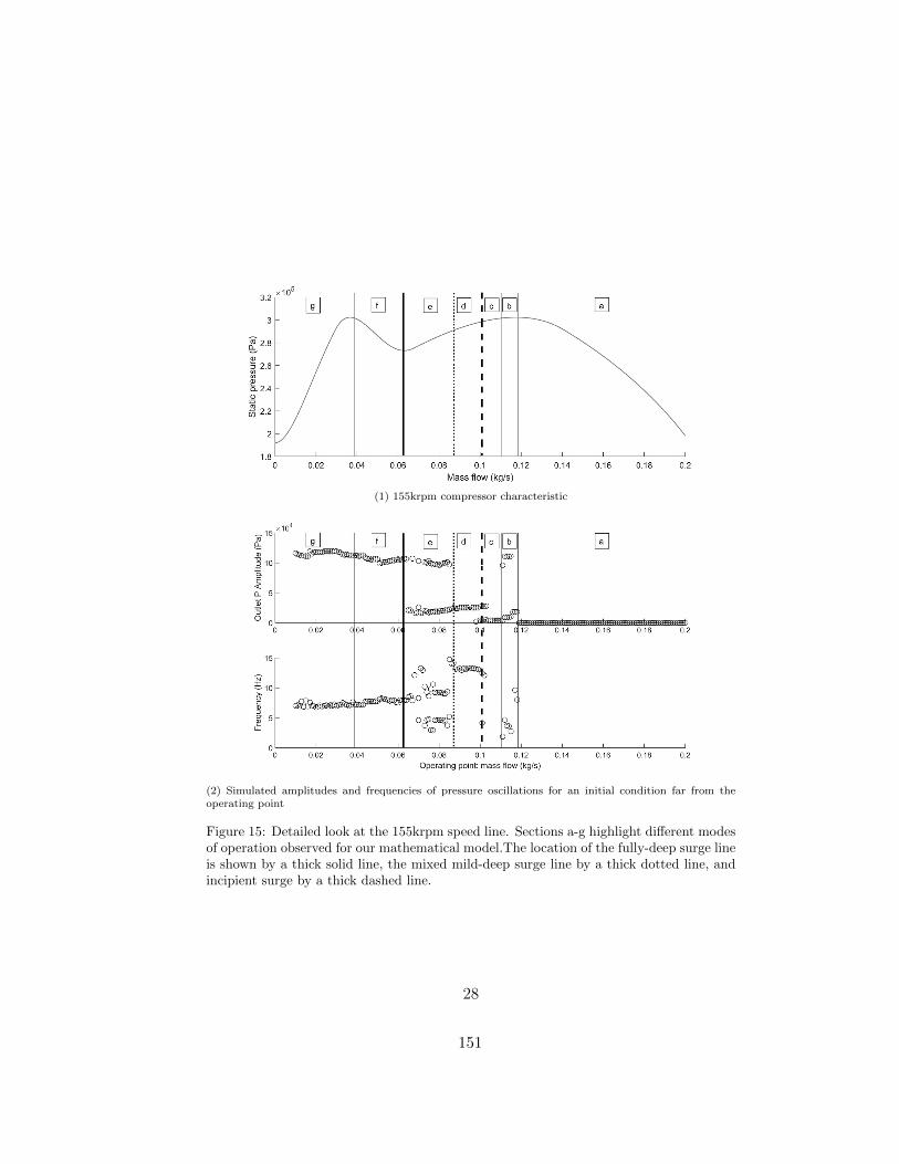
(1) 155krpm compressor characteristic
(2) Simulated amplitudes and frequencies of pressure oscillations for an initial condition far from theoperating point
Figure 15: Detailed look at the 155krpm speed line. Sections a-g highlight different modesof operation observed for our mathematical model.The location of the fully-deep surge lineis shown by a thick solid line, the mixed mild-deep surge line by a thick dotted line, andincipient surge by a thick dashed line.
28
151
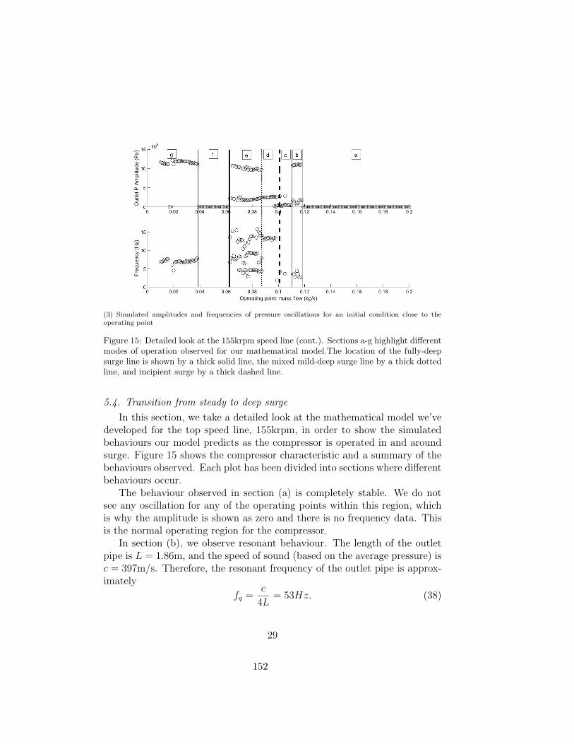
(3) Simulated amplitudes and frequencies of pressure oscillations for an initial condition close to theoperating point
Figure 15: Detailed look at the 155krpm speed line (cont.). Sections a-g highlight differentmodes of operation observed for our mathematical model.The location of the fully-deepsurge line is shown by a thick solid line, the mixed mild-deep surge line by a thick dottedline, and incipient surge by a thick dashed line.
5.4. Transition from steady to deep surge
In this section, we take a detailed look at the mathematical model we’vedeveloped for the top speed line, 155krpm, in order to show the simulatedbehaviours our model predicts as the compressor is operated in and aroundsurge. Figure 15 shows the compressor characteristic and a summary of thebehaviours observed. Each plot has been divided into sections where differentbehaviours occur.
The behaviour observed in section (a) is completely stable. We do notsee any oscillation for any of the operating points within this region, whichis why the amplitude is shown as zero and there is no frequency data. Thisis the normal operating region for the compressor.
In section (b), we observe resonant behaviour. The length of the outletpipe is L = 1.86m, and the speed of sound (based on the average pressure) isc = 397m/s. Therefore, the resonant frequency of the outlet pipe is approx-imately
fq =c
4L= 53Hz. (38)
29
152
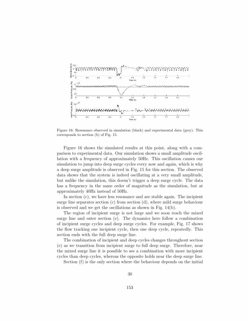
Figure 16: Resonance observed in simulation (black) and experimental data (grey). Thiscorresponds to section (b) of Fig. 15.
Figure 16 shows the simulated results at this point, along with a com-parison to experimental data. Our simulation shows a small amplitude oscil-lation with a frequency of approximately 50Hz. This oscillation causes oursimulation to jump into deep surge cycles every now and again, which is whya deep surge amplitude is observed in Fig. 15 for this section. The observeddata shows that the system is indeed oscillating at a very small amplitude,but unlike the simulation, this doesn’t trigger a deep surge cycle. The datahas a frequency in the same order of magnitude as the simulation, but atapproximately 40Hz instead of 50Hz.
In section (c), we have less resonance and are stable again. The incipientsurge line separates section (c) from section (d), where mild surge behaviouris observed and we get the oscillations as shown in Fig. 14(b).
The region of incipient surge is not large and we soon reach the mixedsurge line and enter section (e). The dynamics here follow a combinationof incipient surge cycles and deep surge cycles. For example, Fig. 17 showsthe flow tracking one incipient cycle, then one deep cycle, repeatedly. Thissection ends with the full deep surge line.
The combination of incipient and deep cycles changes throughout section(e) as we transition from incipient surge to full deep surge. Therefore, nearthe mixed surge line it is possible to see a combination with more incipientcycles than deep cycles, whereas the opposite holds near the deep surge line.
Section (f) is the only section where the behaviour depends on the initial
30
153

Figure 17: Simulated mass flow and pressure for the transition period between incipientand deep surge.This corresponds to section (e) of Fig. 15.
condition of the simulation. We have two possible behaviours in this region.The first is full deep surge as seen in Fig. 15(2), and the second is steadybehaviour as seen in Fig. 15(3).
We can plot these two behaviours in the mass flow - pressure plane (seeFig. 18) to get a better understanding of what is happening. This showsus that there is a region (shaded grey) close to the operating point (theintersection between throttle and compressor characteristics) that if we startthe simulation within we will see stable behaviour. Outside of this region,we will observe deep surge.
Having two possible dynamics occur at the same operating point cancause some really interesting behaviour. If region (f) is observed as stable, iteffectively moves the deep surge line to the beginning of section (g). There-fore, it explains why quiet periods can occur between incipient and deepsurge.
Figure 19 show some experimental data from Cummins Turbo Technolo-gies where this quiet period is observed. However, it is not always observedand sometimes repeat tests will give different answers, which can cause diffi-culties when trying to determine the deep surge limit. This is the first timethat this observed behaviour has been predicted and explained by surge mod-elling. Furthermore, being aware of the existence of two possible behavioursin region (f) is of key importance as it will help designers to determine more
31
154
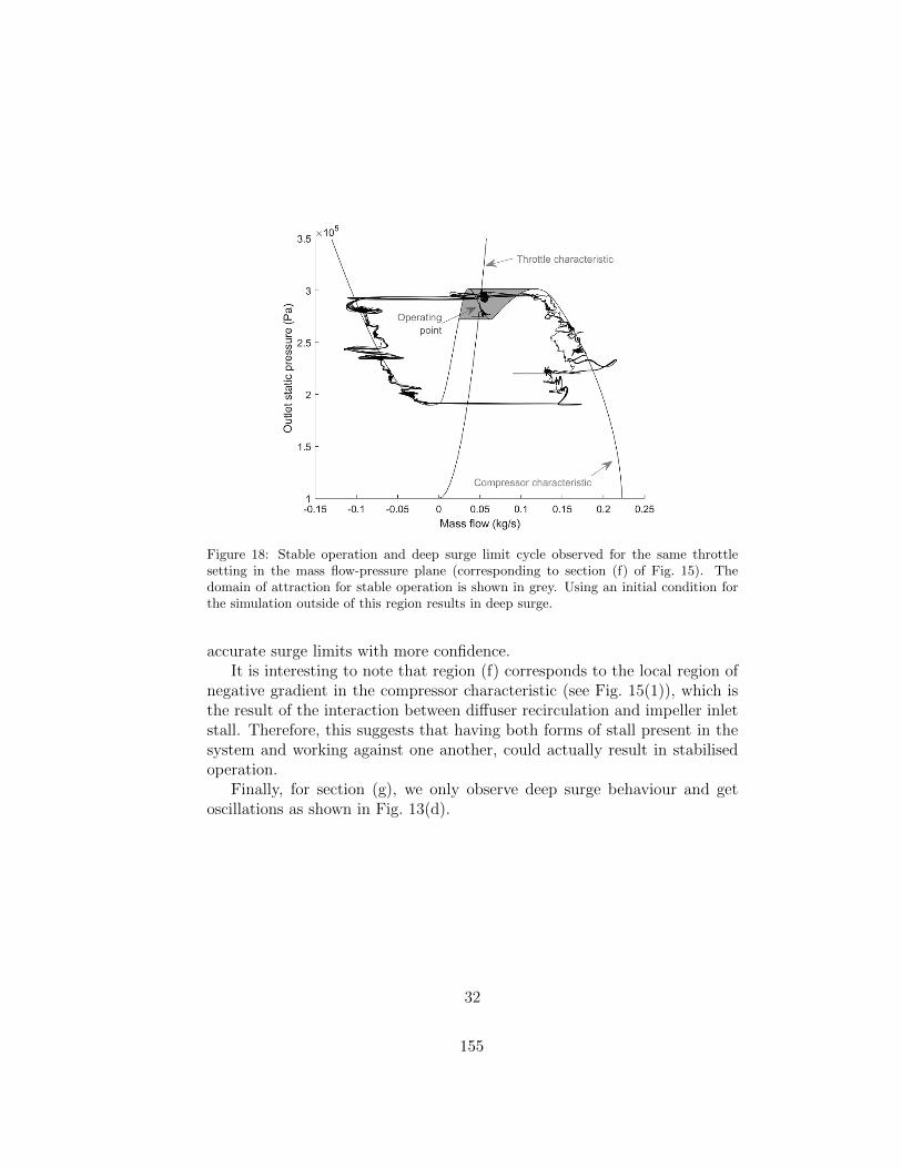
Figure 18: Stable operation and deep surge limit cycle observed for the same throttlesetting in the mass flow-pressure plane (corresponding to section (f) of Fig. 15). Thedomain of attraction for stable operation is shown in grey. Using an initial condition forthe simulation outside of this region results in deep surge.
accurate surge limits with more confidence.It is interesting to note that region (f) corresponds to the local region of
negative gradient in the compressor characteristic (see Fig. 15(1)), which isthe result of the interaction between diffuser recirculation and impeller inletstall. Therefore, this suggests that having both forms of stall present in thesystem and working against one another, could actually result in stabilisedoperation.
Finally, for section (g), we only observe deep surge behaviour and getoscillations as shown in Fig. 13(d).
32
155
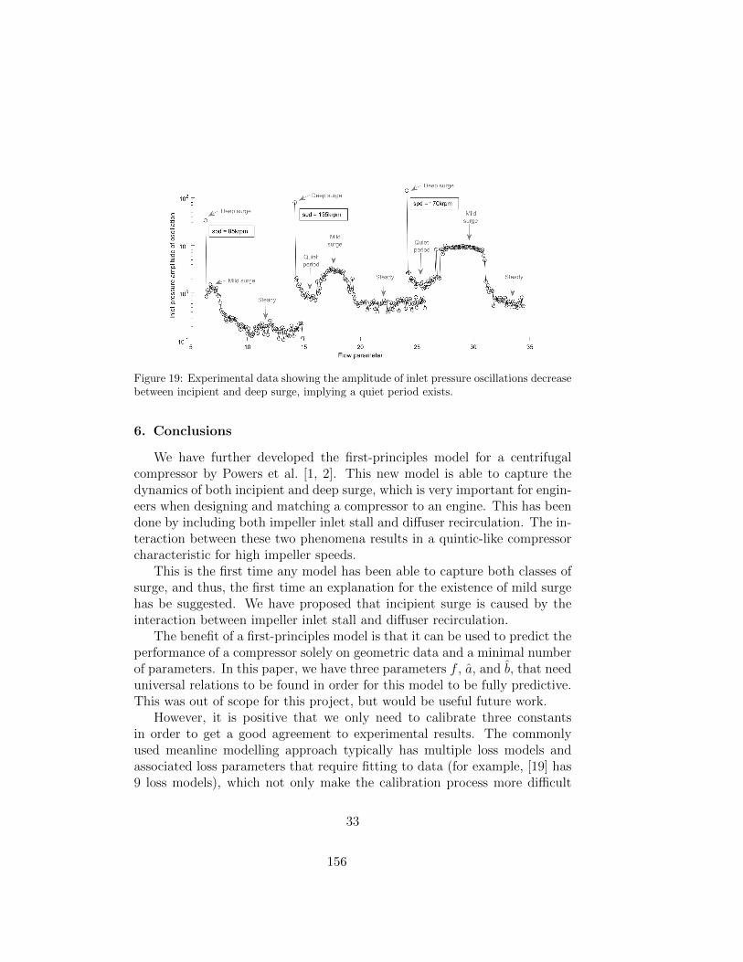
Figure 19: Experimental data showing the amplitude of inlet pressure oscillations decreasebetween incipient and deep surge, implying a quiet period exists.
6. Conclusions
We have further developed the first-principles model for a centrifugalcompressor by Powers et al. [1, 2]. This new model is able to capture thedynamics of both incipient and deep surge, which is very important for engin-eers when designing and matching a compressor to an engine. This has beendone by including both impeller inlet stall and diffuser recirculation. The in-teraction between these two phenomena results in a quintic-like compressorcharacteristic for high impeller speeds.
This is the first time any model has been able to capture both classes ofsurge, and thus, the first time an explanation for the existence of mild surgehas be suggested. We have proposed that incipient surge is caused by theinteraction between impeller inlet stall and diffuser recirculation.
The benefit of a first-principles model is that it can be used to predict theperformance of a compressor solely on geometric data and a minimal numberof parameters. In this paper, we have three parameters f , a, and b, that needuniversal relations to be found in order for this model to be fully predictive.This was out of scope for this project, but would be useful future work.
However, it is positive that we only need to calibrate three constantsin order to get a good agreement to experimental results. The commonlyused meanline modelling approach typically has multiple loss models andassociated loss parameters that require fitting to data (for example, [19] has9 loss models), which not only make the calibration process more difficult
33
156
but also reduces the models predictive ability as it has a higher dependenceon experimental or CFD data.
We then developed a non-linear test-rig model in which we can use thecompressor characteristics developed in this paper, and this was validatedvia experiments conducted at the University of Bath.
We have shown a great fit between simulation and data for incipient anddeep surge oscillations, for all impeller speeds. We are able to capture a lotof the details in the experimental data signals for mass flow and pressure.There is some minor miss-match with frequency of ±1Hz, but the oscillationfrequency always remains in the correct order of magnitude.
At low impeller speeds, diffuser recirculation is not triggered and we re-turn to the cubic-like shape of compressor characteristic commonly seen inliterature. Since incipient surge is only simulated with the quintic-like shape,we do not simulate mild surge for the lower speeds. This agrees with the data,as incipient surge was only observed for high impeller rotational speeds.
We have shown the range of behaviours that can be simulated by our testrig model for the 155krpm speed line. We were able to capture resonance,incipient surge, transitions between mild and deep surge, deep surge, and thepotential for a quiet period between incipient and deep surge.
Observing that our model can simulate both stable operation and deepsurge for the same throttle setting, helps to explain the quietening phe-nomenon where a stable region is sometimes observed between incipient anddeep surge operation. The behaviour of the mathematical model in thisregion depends on the initial conditions given to it, which explains why re-peated experiments can result in observing different surge behaviour for thisregion.
This model has huge potential for helping centrifugal compressor man-ufacturers. The mathematical models have a great predictive ability andare able to capture the dynamics observed in and around surge to remark-able detail. Also, by extending the test-rig model to a model of an engine,it is possible to use the compressor characteristics to predict the on-engineperformance of a compressor and the location of the surge limits for thatpipework.
Furthermore, this is the first time incipient surge and the potential fora quiet periods have been predicted in a model. This has allowed us topropose explanations for the existence of such phenomena where one did notexist before.
34
157

Acknowledgements
Katherine Powers is supported by a scholarship from the EPSRC Centrefor Doctoral Training in Statistical Applied Mathematics at Bath (SAMBa),under the project EP/L015684/1.
References
[1] K. H. Powers, C. J. Brace, C. J. Budd, C. D. Copeland, P. A. Milewski,Modeling axisymmetric centrifugal compressor characteristics from firstprinciples, Journal of Turbomachinery 142 (9) (2020) 091010(11 pages).
[2] K. H. Powers, I. J. Kennedy, C. J. Brace, P. A. Milewski, C. D. Copeland,Development and validation of a model for centrifugal compressors inreversed flow regimes, in: ASME Turbo Expo 2020: TurbomachineryTechnical Conference and Exposition, American Society of MechanicalEngineers Digital Collection, 2020.
[3] R. Stone, Introduction to internal combustion engines, 4th Edition, Pal-grave MacMillan, 2012.
[4] N. Watson, M. S. Janota, Turbocharging: The internal combustion en-gine, MacMillan, 1982.
[5] D. A. Fink, Surge dynamics and unsteady flow in centrifugal com-pressors, Ph.D. thesis, Massachusetts Institute of Technology (1988).
[6] I. Day, Stall, surge, and 75 years of research, Journal of Turbomachinery138 (1) (2016) 011001.
[7] M. C. Huppert, W. Benser, Some stall and surge phenomena in axial-flow compressors, Journal of the Aeronautical Sciences 20 (12) (1953)835–845.
[8] H. Emmons, C. Pearson, H. Grant, Compressor surge and stall propaga-tion, Trans. of the ASME 77 (4) (1955) 455–467.
[9] E. M. Greitzer, Surge and rotating stall in axial flow compressors - PartI: Theoretical compression system model, Journal of Engineering forPower 98 (2) (1976) 190–198.
35
158
[10] C. Hos, A. Champneys, L. Kullmann, Bifurcation analysis of surge androtating stall in the Moore–Greitzer compression system, IMA Journalof Applied Mathematics 68 (2) (2003) 205–228.
[11] S. G. Koff, E. M. Greitzer, Stalled flow performance for axial com-pressors: I - Axisymmetric characteristic, in: 29th International GasTurbine Conference and Exhibit, Vol. 1, American Society of Mechan-ical Engineers, 1984.
[12] F. K. Moore, E. M. Greitzer, A theory of post-stall transients in axialcompression systems: Part I - Development of equations, Journal ofEngineering for Gas Turbines and Power 108 (1) (1986) 68–76.
[13] J. Galindo, J. Serrano, H. Climent, A. Tiseira, Experiments and mod-elling of surge in small centrifugal compressor for automotive engines,Experimental Thermal and Fluid Science 32 (3) (2008) 818–826.
[14] R. L. Elder, M. E. Gill, A discussion of the factors affecting surge incentrifugal compressors, Journal of Engineering for Gas Turbines andPower 107 (1985) 499–506.
[15] G. Martin, V. Talon, P. Higelin, A. Charlet, C. Caillol, Implementingturbomachinery physics into data map-based turbocharger models, SAEInternational Journal of Engines 2 (1) (2009) 211–229.
[16] D. Japikse, Centrifugal compressor design and performance, Vol. 2, Con-cepts Eti White River Junction, VT, 1996.
[17] E. Sundstrom, M. Mihaescu, M. Giachi, E. Belardini, V. Michelassi,Analysis of vaneless diffuser stall instability in a centrifugal compressor,International Journal of Turbomachinery, Propulsion and Power 2 (4)(2017) 19.
[18] A. N. Abdelhamid, Analysis of rotating stall in vaneless diffusers of cent-rifugal compressors, in: ASME 1980 International Gas Turbine Confer-ence and Products Show, ASME, 1980.
[19] H. W. Oh, E. S. Yoon, M. Chung, An optimum set of loss models forperformance prediction of centrifugal compressors, Proceedings of theInstitution of Mechanical Engineers, Part A: Journal of Power and En-ergy 211 (4) (1997) 331–338.
36
159
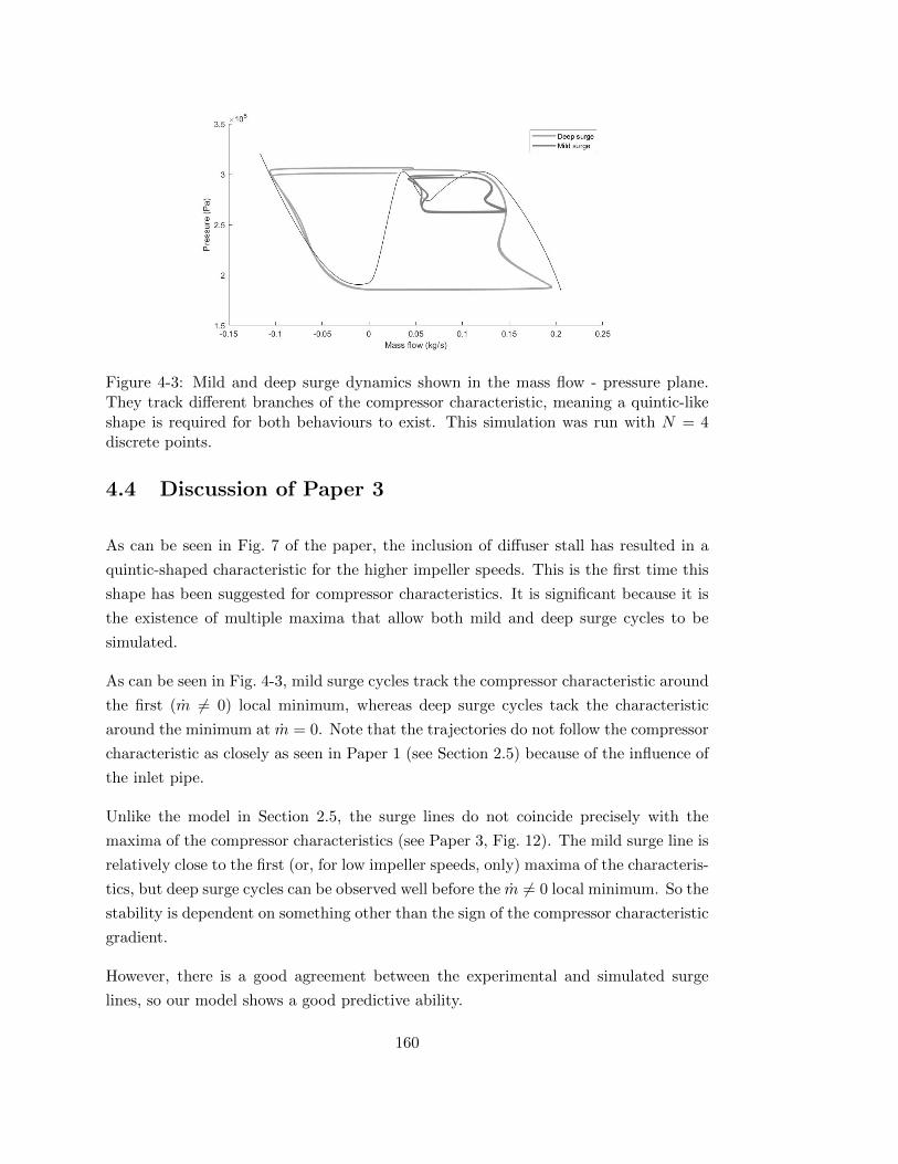
Figure 4-3: Mild and deep surge dynamics shown in the mass flow - pressure plane.They track different branches of the compressor characteristic, meaning a quintic-likeshape is required for both behaviours to exist. This simulation was run with N = 4discrete points.
4.4 Discussion of Paper 3
As can be seen in Fig. 7 of the paper, the inclusion of diffuser stall has resulted in a
quintic-shaped characteristic for the higher impeller speeds. This is the first time this
shape has been suggested for compressor characteristics. It is significant because it is
the existence of multiple maxima that allow both mild and deep surge cycles to be
simulated.
As can be seen in Fig. 4-3, mild surge cycles track the compressor characteristic around
the first (m 6= 0) local minimum, whereas deep surge cycles tack the characteristic
around the minimum at m = 0. Note that the trajectories do not follow the compressor
characteristic as closely as seen in Paper 1 (see Section 2.5) because of the influence of
the inlet pipe.
Unlike the model in Section 2.5, the surge lines do not coincide precisely with the
maxima of the compressor characteristics (see Paper 3, Fig. 12). The mild surge line is
relatively close to the first (or, for low impeller speeds, only) maxima of the characteris-
tics, but deep surge cycles can be observed well before the m 6= 0 local minimum. So the
stability is dependent on something other than the sign of the compressor characteristic
gradient.
However, there is a good agreement between the experimental and simulated surge
lines, so our model shows a good predictive ability.
160

In the paper, the PDEs for the compression system (Eqs. 33 and 34) have an additional
term to the ones we derived in Section 4.1. This is because, on programming Eqs. 4.1.1-
4.1.2, we observed high-frequency growing oscillations that are often found in numerical
solutions to PDEs. To remove these unphysical oscillations, we needed to incorporate
some form of damping.
Therefore, we chose to include some viscous dissipation into the model. Recall from
Section 2.1, that the fundamental equations of motion with stresses and viscous dissi-
pation are
∂ρ
∂t+∇ · (ρu) = 0, (4.4.1)
∂
∂t(ρu) +∇ · (ρ(u⊗ u)) = −∇p+∇ · τ, (4.4.2)
∂
∂t(ρE) +∇ · (ρuE + pu)−∇ · (τ · u) = 0. (4.4.3)
Recall also that viscous dissipation can be decomposed into two parts
∇ · (τ · u) = u · (∇ · τ)− τ : ∇u. (4.4.4)
By assuming τ : ∇u = 0 and just including dissipation in the form of the first term,
we can retain the isentropic flow assumption.
To see this, notice that subtracting conservation of momentum dotted with u from the
conservation of energy will cause the u · (∇ · τ) terms to cancel so we can follow the
same procedure as in Section 2.2 (Eqs. 2.2.6 - 2.2.11) to obtain the isentropic relation
p = κργ .
When modelling the steady-state behaviour of the compressor, we have chosen to model
∇·τ as a friction term, F . Therefore, to be consistent with this approach, so we decided
to include a viscous dissipation term of
∇ · (τ · u) = u · (∇ · τ) =f
2ρ|u|3S, (4.4.5)
which resulted in Eqs. 33 and 34 in the paper.
The simulation results of this PDE model with dissipation have a remarkable fit to the
experimental data. This is especially true for simulating deep surge (Paper 3, Fig. 13)
where we are able to capture the shapes of the mass flow, outlet pressure, and inlet
pressure traces to considerable detail.
161
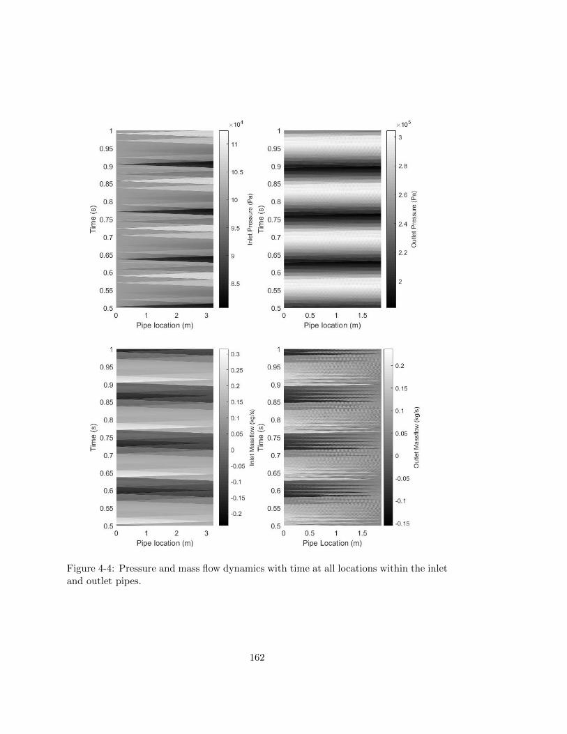
Figure 4-4: Pressure and mass flow dynamics with time at all locations within the inletand outlet pipes.
162
Moreover, the advantage of having a model that has both a time and spacial dimension,
is that we can capture the wave dynamics within the pipework. Figure 4-4, shows how
the pressure and mass flow at all spatial locations within the pipework vary with time.
Here, we can see a series of triangles. These are waves travelling from one end of the
pipe to the other at the speed of sound, a. We can see from this that the period of a
surge oscillation is an integer multiple of the time it takes for these waves to travel, i.e.La , where L is the length of the pipe.
To try and understand the period (and hence frequency) of the simulated surge oscil-
lations, consider the simple case where N = 4 and the system is a linearised, so
∂m1
∂t=
A
L1(pamb − p2), (4.4.6)
∂p2
∂t=
a21
AL1(m1 − m3), (4.4.7)
∂m3
∂t=
A
L2(pc(m3)− p4), (4.4.8)
∂p4
∂t=
a22
AL2(m3 − mT (p4)), (4.4.9)
where a1, a2 are constant values for speed of sound for the inlet and outlet pipes
depending on the average of p2 and p4 respectively.
As seen in Fig. 4-5(a), fast and slow dynamics are observed when plotting inlet mass
flow against outlet pressure. The slow dynamics occur when the trajectory follows
the compressor characteristic closely, and the fast dynamics occur when the trajectory
switches from one branch of the compressor characteristic to another.
Thus, a reasonable approximation for the period of oscillation is the sum of the time
taken for the slow dynamics (i.e. T↑ and T↓ in Fig. 4-5(b)). The slow dynamics occur
when the change in mass flow is small and so Eqs. 4.4.7 and 4.4.9 dominate. Eliminating
m3 in these gives:
d
dt
(p4 +
a22L1
a21L2
p2
)=
a22
AL2(m1 − mT (p4)). (4.4.10)
We can get an approximation to T↑ by replacing the mass flow values with their average
163

Figure 4-5: (a) Deep surge trajectory in the mass flow - pressure plane. The dynamics isvery fast when moving between branches of the compressor characteristic. (b) Diagramused to find an approximation for the period of surge oscillation.
(m↑ and mT in Fig. 4-5(b)), and approximating the derivative. This gives
∆P +a22L1
a21L2∆Pin
T↑≈ a2
2
AL2(m↑ − mT ), (4.4.11)
and so, on rearranging for T↑, we have
T↑ ≈(AL2∆P
a22
+AL1∆Pin
a21
)1
m↑ − mT(4.4.12)
where ∆P is the change in outlet pressure shown in Fig. 4-5(b), and ∆Pin is the
change in inlet pressure. This is typically a lot smaller than ∆P (e.g. Fig. 4-4 shows
us ∆P ≈ 1bar and ∆Pin ≈ 0.4bar), but will still impact the period of oscillation.
Similarly, for T↓ we have
T↓ ≈ −(AL2∆P
a22
+AL1∆Pin
a21
)1
m↓ − mT. (4.4.13)
Therefore, combining these for the period T ≈ T↑ + T↓ results in
T ≈ (m↑ − m↓)(m↑ − mT )(mT − m↓)
(A∆P
a2
L2
a2+A∆Pina1
L1
a1
). (4.4.14)
Notice that L1a1
and L2a2
are the lengths of time it takes for information to travel down
the inlet and outlet pipes respectively. Therefore, the true period is likely to be an
integer linear combination of these that is the close to the above approximation.
164
Furthermore, assuming there is no inlet pipe (and hence ∆Pin = 0) will result in a
smaller period (higher frequency). So the inlet pipework actually lowers the observed
frequency of oscillation, and explains why models without the inlet pipework can strug-
gle to match the observed surge dynamics.
This relation also tells us that the larger the surge amplitude, both in pressure, ∆P ,
and mass flow, ∆m = m↑ − m↓, results in a longer period (as hence lower frequency).
This agrees with the observation of mild surge having a higher frequency than deep
surge.
Also, this relation tells us that an increase in pipe cross-sectional area, or length, will
result in a longer period (lower frequency). This agrees with what we saw in Section
2.5.
Finally, notice that we can approximate the change dynamic pressure 12∆(ρu2) by
1
2∆(ρu)u =
1
2
∆m
Au, (4.4.15)
where u is the average velocity in the pipe. Therefore, we could write the period as
T ≈ 1
2∆mT2
(1
Ma2
∆P12∆(ρu2)
L2
a2+
1
Ma1
∆Pin12∆(ρu2
in)
L1
a1
)(4.4.16)
where
∆mT =
√(m↑ − mT
m↑ − m↓
)(mT − m↓m↑ − m↓
)(4.4.17)
is the geometric mean of the distance between m↑, m↓ and the throttle mass flow.
Therefore, we can expect the period of oscillation to be impacted by the throttle setting,
the Mach number in both pipes, and the ratio of static to dynamic pressure in each
pipe.
These approximations show us that the frequency of observed compressor surge is a
complex process that is influenced by many variables. Therefore, it is not surprising
that our model cannot always accurately predict the frequency of oscillation observed
in experimental measurements of surge.
165
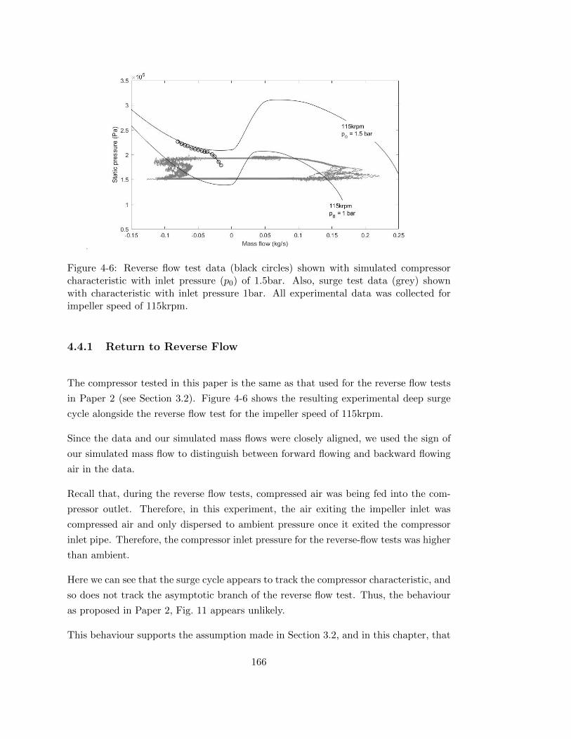
Figure 4-6: Reverse flow test data (black circles) shown with simulated compressorcharacteristic with inlet pressure (p0) of 1.5bar. Also, surge test data (grey) shownwith characteristic with inlet pressure 1bar. All experimental data was collected forimpeller speed of 115krpm.
4.4.1 Return to Reverse Flow
The compressor tested in this paper is the same as that used for the reverse flow tests
in Paper 2 (see Section 3.2). Figure 4-6 shows the resulting experimental deep surge
cycle alongside the reverse flow test for the impeller speed of 115krpm.
Since the data and our simulated mass flows were closely aligned, we used the sign of
our simulated mass flow to distinguish between forward flowing and backward flowing
air in the data.
Recall that, during the reverse flow tests, compressed air was being fed into the com-
pressor outlet. Therefore, in this experiment, the air exiting the impeller inlet was
compressed air and only dispersed to ambient pressure once it exited the compressor
inlet pipe. Therefore, the compressor inlet pressure for the reverse-flow tests was higher
than ambient.
Here we can see that the surge cycle appears to track the compressor characteristic, and
so does not track the asymptotic branch of the reverse flow test. Thus, the behaviour
as proposed in Paper 2, Fig. 11 appears unlikely.
This behaviour supports the assumption made in Section 3.2, and in this chapter, that
166
we have a continuous compressor characteristic. It also suggests that the asymptotic
behaviour seen in the reversed flow tests is likely to be linked to the behaviour of the
system as a whole. For example, as seen in Fig. 3-5, the throttle characteristic has a
very steep gradient, and so the behaviour could be explained if the system switches
from following the compressor characteristic to following the throttle characteristic for
small negative mass flows.
4.5 Conclusions
In this chapter we have further developed the steady-state compressor characteristic so
that it includes diffuser recirculation. This has resulted in a quintic-shaped character-
istic that has the ability to capture both mild and deep surge.
We also used the PDE form of the reduced order surge model created in Section 2.2
and solved this over a staggered grid. The staggered grid formulation provided us with
a simple way to transform between the PDEs and the ODE system used in the previous
two chapters.
We get excellent agreement to experimental data for mass flow and pressure traces at
a variety of different impeller speeds. We have some difficulty in accurately predicting
the correct frequency of oscillation. However, after a more detailed look into what
affects the period of a surge oscillation, it is clear that this is sensitive to many factors
and so it is unsurprising that a simple reduced model would have difficulty capturing
this.
We also see a good ability of the model to predict the onset of both mild and deep
surge. This implies that our reduced order model now contains the most important
dynamics to simulate this physical phenomena.
We have seen that the addition of inlet pipework has some interesting effects on the
simulated dynamics. Figure 4-3 shows us that the trajectories do not follow the com-
pressor characteristic as closely when the inlet pipe is modelled. The inlet pipe also
reduces the simulated frequency of oscillation.
Another thing to note is that, while exploring the effect inlet pressure has on the
compressor characteristics, the following relation was discovered:
pM+1 = pc
([pambpM
]mM+1, pamb
)pMpamb
. (4.5.1)
167
Since this was discovered by simulation, mathematical investigation is needed to vali-
date this result. However, this result is interesting because it means that the compres-
sor characteristic ODEs only need to be computed using ambient inlet pressure. This
would help with computational efficiency of the PDE model presented in the paper, as
the compressor characteristic ODEs need not been solved each time the pc boundary
condition is implemented.
Finally, we compared the results from the surge tests conducted in this Section 4.3 to
the reverse flow test in Section 3.2. Since the surge results have such a good fit while
using a continuous characteristic, it appears likely that the deviation of the reverse flow
tests from the characteristic is related to a system level phenomenon, rather than the
shape of the characteristic itself.
Now we have developed a model which captures the dynamics of surge with good
results, we can start to dig deeper into the mathematical properties of the model itself.
In particular, looking into conditions for the switch of stability is vital information
when trying to predict the location of surge limits.
168
Chapter 5
Stability Analysis of Surge Model
In all three papers (Sections 2.5, 3.2 and 4.3) we have observed that the stability of the
system appears to be dependent on the gradient of the compressor characteristic. In
particular, when the gradient of the compressor characteristic is negative, the system
appears to always be stable.
In order to understand this dependence further, we can perform more formal stability
analysis on our surge model.
5.1 Selected Model for Analysis
We wish to analyse a system which captures the main dynamics of surge, but is simple
enough that the analytical calculations are manageable. Therefore, we shall return to
the ODE model developed in Section 2.2:
dm
dt=A
L(pc(m)− p) +
κ1γ
AL
(m2
pc(m)1γ
− mT (p)2
p1γ
)≡ f(m, p), (5.1.1)
dp
dt=γκ
1γ
ALpγ−1γ (m− mT (p)) ≡ g(m, p). (5.1.2)
The results from analysing this model will still be applicable to the PDE model in
Section 4.1 since this is the case where N = 2 and we have no inlet pipe.
As noted in Section 4.4, the inlet pipe does influence the behaviour of the system, and
169

is therefore likely to have some influence on the system stability. However, surge is
still observed in the case with no inlet pipe and so we should be able to identify the
key variables which control the onset of surge instabilities without including this in the
stability analysis.
For the compressor characteristic, we shall use the model developed in Section 4.3 as
this will enable us to understand both mild surge and deep surge stability.
For the throttle characteristic, we shall use an incompressible version of that developed
in Section 2.3, i.e.
mT = sgn(p− pamb)√
2γ
γ − 1A2ρamb
µ2
1− µ2|p− pamb|, (5.1.3)
to make analytical computations involving this simpler. For our analysis, we shall
only consider p > pamb as this means the compressor is functioning as expected and
generating pressure within the pipework. Therefore this can be written as
mT = (σf(µ)(p− pamb))12 (5.1.4)
for a constant
σ =2γ
γ − 1A2ρamb, (5.1.5)
and function
f(µ) =µ2
1− µ2, (5.1.6)
where µ is the throttle parameter.
We have observed that by closing the throttle, we can see a switch of stability that
corresponds to the onset of surge. Therefore, we wish to understand how our system
changes with the behaviour of the parameter µ.
Let x = (m, p)T and F(·) = (f(·), g(·))T . Then our system can be written as x = F(x)
where x denotes differentiation with respect to t.
5.2 Equilibrium Points
The first step in stability analysis is finding the equilibrium (or stationary) points of
the system. These are points which remain unchanged by the differential equations, so
170
if the system was given an initial condition of an equilibrium point, it would remain
there for all time.
Let x∗ be an equilibrium point. Then x∗ = F(x∗) = 0, which implies f(m∗, p∗) =
g(m∗, p∗) = 0.
For our system, if g(m, p) = 0 then either p = 0 or m = mT (p).
Now, p = 0 is outside our domain of interest as pamb > 0. However, there is no
equilibrium point here as f →∞ as p→ 0 because, from Eq. 5.1.4, we have
m2T
p1γ
= σf(µ)
(pγ−1γ − pamb
p1γ
)→ −∞ (5.2.1)
as p→ 0.
If m = mT (p), then f(m, p) = 0 when
A
L(pc(m)− p) +
m2κ1γ
AL
(1
pc(m)1γ
− 1
p1γ
)= 0, (5.2.2)
which is true when p = pc(m).
Therefore, the system has an equilibrium point at (m∗, p∗) where m∗ = mT (p∗) and
p∗ = pc(m∗).
As seen in previous chapters, the intersection between the compressor characteristic and
the throttle characteristic is the operating point of the compression system. Therefore,
this tells us the operating point is an equilibrium point. This makes sense because
when the system is stable it tends to the operating point, and once there it remains
there for all time.
The next step is therefore to determine when this equilibrium is stable, which would
mean the compression system operates in a stable manner.
171
5.3 Linear Stability Analysis
To determine the stability of an equilibrium point, we want to study the behaviour of
nearby points, i.e. x = x∗ + y for small y. Differentiating gives x = y and
x = F(x∗ + y) =:0
F(x∗) +DF(x∗)y +O(|y|2) (5.3.1)
by Taylor expanding around x∗, where the matrix of partial derivatives, DF, is termed
the Jacobian [60]. Therefore, studying the linear system
y = DF(x∗)y (5.3.2)
will give us a reasonable idea of the behaviour of y = x− x∗ [60].
In the case of a non-singular Jacobian, the solution of Eq. 5.3.2 is
y(t) =n∑
i=1
yieλit, (5.3.3)
where (λi,yi) are eigenvalue - eigenvector pairs of the system. This tells us that, in
the direction of eigenvector yi, the solution is either growing or shrinking exponentially
dependent on the sign of λi [61]. Therefore:
If all eigenvalues have negative real part, y→ 0, and so x→ x∗ and the equilib-
rium point is stable.
If all eigenvalues have positive real part, y → ∞, so x grows away from x∗ and
the equilibrium point is unstable.
If we have a mix of positive and negative real parts, y will shrink exponentially in
some directions and grow exponentially in others. This is called a saddle point,
and the equilibrium point is unstable.
Moreover, if the eigenvalue has a non-zero imaginary part, the behaviour is oscillatory
in nature [61]. So we will have growing or shrinking spiral behaviour.
172

5.3.1 Computing the Jacobian
For our case, denote the Jacobian by J , then
J∗ =
(∂f∂m
∂f∂p
∂g∂m
∂g∂p
)∣∣∣∣∣(m∗,p∗)
. (5.3.4)
Differentiating Eqs. 5.1.1 and 5.1.2 gives
∂f
∂m=A
L
dpcdm
+κ
1γ
AL
(2m
pc(m)1γ
− m2
γpc(m)γ+1γ
dpcdm
), (5.3.5)
∂f
∂p= −A
L− κ
1γ
AL
(2mT (p)
p1γ
dmT
dp+mT (p)2
γpγ+1γ
), (5.3.6)
∂g
∂m=γκ
1γ
ALpγ−1γ , (5.3.7)
∂g
∂p=γκ
1γ
AL
(γ − 1
γ
(m− mT (p))
p1γ
− pγ−1γdmT
dp
), (5.3.8)
so evaluating at (m∗, p∗) results in
(∂f
∂m
)∗=
(A
L− κ
1γ
γAL
m∗2
p∗ γ+1
γ
)dpcdm
(m∗) +2κ
1γ
AL
m∗
p∗ 1γ
, (5.3.9)
(∂f
∂p
)∗= −2κ
1γ
AL
m∗
p∗ 1γ
dmT
dp(p∗)−
(A
L− κ
1γ
γAL
m∗2
p∗ γ+1
γ
), (5.3.10)
(∂g
∂m
)∗=γκ
1γ
ALp∗ γ−1
γ , (5.3.11)
(∂g
∂p
)∗= −γκ
1γ
ALp∗ γ−1
γdmT
dp(p∗). (5.3.12)
In Section 2.2, we determined that the system was isentropic so p = κργ (see Eq.
2.2.37). We can also write a2 = γpρ due to Eq. 2.2.47, and u = m
Aρ by definition of mass
flow rate. Therefore, the above can be simplified to get
(∂f
∂m
)∗=A
L
(1− u∗2
a∗2
)dpcdm
(m∗) +2u∗
L, (5.3.13)
173

(∂f
∂p
)∗= −2u∗
L
dmT
dp(p∗)− A
L
(1− u∗2
a∗2
), (5.3.14)
(∂g
∂m
)∗=a∗2
AL, (5.3.15)
(∂g
∂p
)∗= −a
∗2
AL
dmT
dp(p∗). (5.3.16)
5.3.2 Determinant-Trace Argument
Since this is a 2D system, we can use the determinant and trace of J∗ to give us stability
criteria. Consider the matrix
A =
(a b
c d
). (5.3.17)
The eigenvalues are solutions of the characteristic polynomial
0 = det(A− λI) =
∣∣∣∣∣a− λ b
c d− λ
∣∣∣∣∣ = λ2 − (trA)λ+ detA, (5.3.18)
where trA = a+ d and detA = ad− bc, are the trace and determinant, respectively.
Let λ1 and λ2 be the eigenvalues, then
λ1,2 =trA±
√trA2 − 4detA
2. (5.3.19)
We can also get from this that λ1 + λ2 = trA and λ1λ2 = detA [61].
From this we know:
detA < 0 means the eigenvalues have opposite signs and we have a saddle.
detA > 0 and trA < 0 means the eigenvalues have negative real part and we have
stability.
detA > 0 and trA > 0 means the eigenvalues have positive real part and the
system is unstable.
4detA > trA2 means we have complex eigenvalues and observe either stable or
unstable oscillatory behaviour.
This is summarised in Fig. 5-1.
174

Figure 5-1: Stability of an equilibrium point in the detA - trA plane, where A is thecorresponding Jacobian [62].
For our Jacobian, the determinant is given by
detJ∗ =1
L2(a∗2 − u∗2)
(1− dpc
dm(m∗)
dmT
dp(p∗)
), (5.3.20)
and the trace is
trJ∗ =A
L
(1− u∗2
a∗2
)dpcdm
(m∗) +2u∗
L− a∗2
AL
dmT
dp(p∗). (5.3.21)
We can see from this that the gradient of both the compressor and throttle characteristic
will play an important role in the stability of the system. Therefore, we will now look
for relations in terms of the gradient of the compressor characteristic, dpcdm , and the
gradient of the throttle characteristic,
dpTdm
=
(dmT
dp
)−1
, (5.3.22)
with the mass flow as the dependent variable. This is because we usually plot charac-
teristics with mass flow on the x-axis and pressure on the y-axis, so the gradients are
easier to understand in this form.
Suppose we have subsonic flow (i.e. u∗ < a∗), then we have stable behaviour when
175

detJ∗ > 0 and trJ∗ < 0, which means
dpTdm
(m∗) >dpcdm
(m∗) (5.3.23)
and
dpTdm
(m∗) <a∗2
A2(
1− u∗2a∗2
)dpcdm (m∗) + 2Au∗
(5.3.24)
respectively.
Similarly, for supersonic flow, stable behaviour occurs if
dpTdm
(m∗) <dpcdm
(m∗) (5.3.25)
anddpTdm
(m∗) <a∗2
2Au∗ −A2(u∗2a∗2 − 1
)dpcdm (m∗)
. (5.3.26)
Finally, we can classify the behaviour as a stable focus if, in addition, 4detJ∗ > (trJ∗)2
holds.
Using the fact that (a+ b)2 = (a− b)2 + 4ab, we can write
(trJ∗)2 =(AL
(1− u∗2
a∗2
)dpcdm −
[2u∗L − a∗2
ALdmTdp
])2+ 4
L2 (a∗2 − u∗2)[
2Au∗a∗2
dpcdm −
dpcdm
dmTdp
]. (5.3.27)
Therefore, 4detJ∗ > (trJ∗)2 can be written as
4
L2(a∗2 − u∗2)
(1− 2Au∗
a∗2dpcdm
)>
(A
L
(1− u∗2
a∗2
)dpcdm− 2u∗
L+a∗2
AL
dmT
dp
)2
. (5.3.28)
Taking square-roots gives us that either of the following hold:
A
L
(1− u∗2
a∗2
)dpcdm− 2u∗
L+a∗2
AL
dmT
dp> −
√4
L2(a∗2 − u∗2)
(1− 2Au∗
a∗2dpcdm
)(5.3.29)
A
L
(1− u∗2
a∗2
)dpcdm− 2u∗
L+a∗2
AL
dmT
dp<
√4
L2(a∗2 − u∗2)
(1− 2Au∗
a∗2dpcdm
). (5.3.30)
176
Therefore, on rearranging for the throttle gradient, we have either of
dpTdm
(m∗) >a∗2
2Au∗ −A2(
1− u∗2a∗2
)dpcdm + 2A
√(a∗2 − u∗2)
(1− 2Au∗
a∗2dpcdm
) , (5.3.31)
dpTdm
(m∗) <a∗2
2Au∗ −A2(
1− u∗2a∗2
)dpcdm − 2A
√(a∗2 − u∗2)
(1− 2Au∗
a∗2dpcdm
) , (5.3.32)
hold if we observe a focus.
5.3.3 Results
All of the stability criteria depends on three things: (i) the gradient of the throttle
characteristic, (ii) the gradient of the compressor characteristic, and (iii) the velocity
of the flow in comparison to the speed of sound.
Figure 5-2 shows how the stability of the system depends on the gradient of the charac-
teristics. The plots were constructed assuming u∗ and a∗ were constant, but the cases
of subsonic and supersonic flow are considered separately.
For subsonic regimes, a negative gradient of the compressor characteristic is almost
always stable, and surge (unstable focus/node) occurs mostly in the positive gradient
region. This is why in Section 2.5 we observed that the switch of stability coincided
with the maximum of the compressor characteristic.
However, our analysis also tells us that, for shallow throttle characteristic gradients,
the switch of stability will occur after the maxima. At higher impeller speeds, the surge
limit occurs at a higher positive mass flow value. Therefore, the gradient of the throttle
characteristic intersecting this point will be shallower than those at lower speeds. This
means we expect surge to occur after the maxima for higher speeds.
Moreover, our analysis tells us the opposite also holds true, i.e. that at lower impeller
speeds the onset of surge can be observed before the maximum of the compressor
characteristic.
For supersonic regimes, we can see that the system is only stable if the compressor
characteristic has a positive gradient. We are only likely to see supersonic flows in the
compression system if we are operating the compressor in choke (i.e. sonic flows are
occurring within the compressor). However, the gradient of the compressor character-
177

Figure 5-2: Stability analysis as the gradient of throttle and compressor characteristicsvary, for constant u∗, a∗ values. (a) shows the subsonic case (u∗ < a∗), and (b) thesupersonic case (u∗ > a∗).
istic tends to negative infinity when operating in choke (see Fig. 1-6 and Fig. 4-5, for
example). Therefore, we would observe a saddle.
178

5.4 Hopf Bifurcation
In Fig. 5-2, we can see that the stability of the system switches from stable to unstable
through the trJ∗ = 0 line. When the system is unstable, we observe surge and so we
expect stable limit cycles to be present in this region.
One way in which limit cycles appear in the system is through a Hopf bifurcation. This
is when an equilibrium point switches its stability at the point where a periodic solution
comes into existence. There is a theorem that can be used to prove the existence of
Hopf bifurcations (see, e.g. [63]).
Theorem 5.1. Hopf Bifurcation Theorem
Consider the planar system x = Fµ(x), written in component form as
x = fµ(x, y),
y = gµ(x, y),
where µ is a parameter. Suppose ∃x∗ such that F(x∗) = 0 and denote the eigenvalues
of the Jacobian DFµ(x∗) by
λ± = α(µ)± iβ(µ).
Suppose further that ∃µ∗ such that
1. Non-hyperbolicity condition: α(µ∗) = 0, β(µ∗) = ω 6= 0, where sgn(ω) = sgn(gx).
2. Transversality condition: dαdµ
∣∣∣∣µ∗
= dH 6= 0.
3. Genericity condition: When the system is written in the form
(x
y
)=
(0 −ωω 0
)(x
y
)+
(f(x, y)
g(x, y)
)
we have that aH 6= 0, where aH = 116(fxxx + fxyy + gxxy + gyyy) + 1
16ω (fxy(fxx +
fyy)− gxy(gxx + gyy)− fxxgxx + fyy gyy).
where the notation
fxy =∂2fµ∂x∂y
∣∣∣∣µ∗
(x∗)
has been used.
179

Then:
a unique curve of periodic solutions bifurcates from x∗ into the region µ > µ∗
(µ < µ∗) if aHdH < 0 (resp. aHdH > 0).
x∗ is a stable fixed point for µ > µ∗ (µ < µ∗) and an unstable fixed point for
µ < µ∗ (µ > µ∗) if dH < 0 (resp. dH > 0).
the periodic solutions have opposite stability to x∗ on the side of µ = µ∗ where
they exist.
Furthermore, the amplitude of the periodic orbits grows like√−dHaH
(µ− µ∗) whilst their
periods tend to 2π|ω| as |µ| → µ∗.
We will use this theorem to look for the existence of Hopf bifurcations for our system
as the parameter in the throttle characteristic, µ, varies.
5.4.1 Non-hyperbolicity
For the non-hyperbolicity condition of Theorem 5.1, recall that the eigenvalues of the
system are
λ1,2 =trJ∗ ±
√(trJ∗)2 − 4detJ∗
2. (5.4.1)
and so we require trJ∗ = 0 and detJ∗ > 0.
From Eq. 5.3.21, trJ∗ = 0 gives us
dmT
dp(p∗) =
A2
a∗2
(1− u∗2
a∗2
)dpcdm
(m∗) + 2Au∗
a∗2. (5.4.2)
Substituting this into Eq. 5.3.20 and simplifying, we get
detJ∗ =
(a∗
L
)2
−(A
L
(1− u∗2
a∗2
)dpcdm
+u∗
L
)2
. (5.4.3)
The non-hyperbolicity condition is satisfied provided this is greater than zero, i.e.
(A
L
(1−Ma2
) dpcdm
+u∗
L
)2
<
(a∗
L
)2
, (5.4.4)
180

which, on rearranging for the compressor characteristic gradient, becomes
− a∗
A(1−Ma)<dpcdm
<a∗
A(1 + Ma)(5.4.5)
where Ma = u∗a∗ is the Mach number.
5.4.2 Transversality
For the transversality condition, we require the derivative of trJ∗ with respect to the
throttle parameter µ to be non-zero at the point where Eq. 5.4.2 holds.
In terms of m∗ = mT (p∗) and p∗, we have
trJ∗ =
(A
L− κ
1γ
γAL
m∗2
p∗ γ+1
γ
)dpcdm
(m∗) +2κ
1γ
AL
m∗
p∗ 1γ
− γκ1γ
ALp∗ γ−1
γdmT
dp(p∗). (5.4.6)
Using the fact that the only variable depending on µ is mT , we can differentiate this
to get
d
dµ(trJ∗) = − 2κ
1γ
γAL
mT
p∗ γ+1
γ
dmT
dµ
dpcdm
+
(A
L− κ
1γ
γAL
m2T
p∗ γ+1
γ
)d2pcdm2
dmT
dµ
+2κ
1γ
AL
1
p∗ 1γ
dmT
dµ− γκ
1γ
ALp∗ γ−1
γd
dµ
(dmT
dp
). (5.4.7)
Recall from Eq. 5.1.4 that mT = (σf(µ)(p− pamb))12 for a constant σ and function
f(µ) = (µ−2 − 1)−1. Therefore, we can use the fact that
f ′(µ) = 2µ−3(µ−2 − 1)−2 =2
µ(1− µ2)f(µ), (5.4.8)
to determine
dmT
dµ=
1
2σ(p− pamb)f ′(µ)(σf(µ)(p− pamb))−
12 =
mT
µ(1− µ2). (5.4.9)
Similarly, differentiating
dmT
dp=
1
2σf(µ) (σf(µ)(p− pamb))−
12 (5.4.10)
181
with respect to µ and using the relation for f ′(µ) gives us
d
dµ
(dmT
dp
)=
1
µ(1− µ2)
dmT
dp. (5.4.11)
Substituting these into Eq. 5.4.7 and grouping terms results in
ddµ(trJ∗) = trJ∗
µ(1−µ2)− 1
µ(1−µ2)
[AL + κ
1γ
γALm∗2
p∗ γ+1γ
]dpcdm +
(AL − κ
1γ
γALm∗2
p∗ γ+1γ
)m∗
µ(1−µ2)d2pcdm2 . (5.4.12)
Therefore, evaluating this at µ∗ (the critical value of µ for which trJ∗ = 0), and writing
this back in terms of u∗ and a∗, we have
dH =1
µ∗(1− µ∗2)
[A
L
(1− u∗2
a∗2
)m∗
d2pcdm2
− A
L
(1 +
u∗2
a∗2
)dpcdm
]. (5.4.13)
Thus, the transversality condition of dH 6= 0 holds provided the compressor character-
istic does not have a point of inflection.
5.4.3 Genericity
Let us write m = x and p = y. The Taylor expansion of x = f(x, y) and y = g(x, y)
are
x = f∗xx+ f∗y y + 12f∗xxx
2 + f∗xyxy + 12f∗yyy
2 + 16f∗xxxx
3 + 12f∗xxyx
2y + 12f∗xyyxy
2 + 16f∗yyyy
3, (5.4.14)
y = g∗xx+ g∗yy + 12g∗xxx
2 + g∗xyxy + 12g∗yyy
2 + 16g∗xxxx
3 + 12g∗xxyx
2y + 12g∗xyyxy
2 + 16g∗yyyy
3, (5.4.15)
where the subscript x or y denotes differentiation with respect to that variable, and ∗denotes evaluation at the equilibrium point x∗ and critical parameter value µ∗.
From Eq. 5.3.5 or 5.3.6 we can see that fxy = 0, and thus fxyy = fxxy = 0. Similarly
Eq. 5.3.7 gives us gxx = 0, and so gxxx = gxxy = 0. Finally, from the non-hyperbolicity
condition we know trJ∗ = 0, which means f∗x = −g∗y . This means Eqs. 5.4.14 and
5.4.15 can be reduced to
x = −g∗yx+ f∗y y +1
2f∗xxx
2 +1
2f∗yyy
2 +1
6f∗xxxx
3 +1
6f∗yyyy
3, (5.4.16)
y = g∗xx+ g∗yy + g∗xyxy +1
2g∗yyy
2 +1
2g∗xyyxy
2 +1
6g∗yyyy
3. (5.4.17)
182
We also know from the non-hyperbolicity condition that, at trJ∗ = 0 the eigenvalues
are given by
λ1,2 = ±√
detJ∗ i = ±√−g∗2y − f∗y g∗x i, (5.4.18)
so we have ω =√−g∗2y − f∗y g∗x.
Since,
− 1
ωf∗y
(g∗y −f∗y−ω 0
)(−g∗y f∗yg∗x g∗y
)(0 f∗yω g∗y
)=
(0 −ωω 0
),
we can change variables to (u, v)T where
(x
y
)=
(0 f∗yω g∗y
)(u
v
)(5.4.19)
and can write our system in the form
(u
v
)=
(0 −ωω 0
)(u
v
)+
(f(u, v)
g(u, v)
), (5.4.20)
where
f(u, v) = g∗xyf∗yuv +
g∗yf∗y
2ω(2g∗xy − f∗xx)v2 +
(g∗yyf∗y − fyy∗g∗y)2ωf∗y
(ωu+ g∗yv)2
+g∗xyyf
∗y
2ω(ωu+ g∗yv)2v −
f∗xxxg∗y(f∗y )2
6ωv3 +
(g∗yyf∗y − fyy∗g∗y)6ωf∗y
(ωu+ g∗yv)3
(5.4.21)
g(u, v) =f∗xxf
∗y
2v2 +
f∗yy2f∗y
(ωu+ g∗yv)2 +f∗yyy6f∗y
(ωu+ g∗yv)3 +f∗xxx(f∗y )2
6v3 (5.4.22)
Therefore, after differentiation and evaluating at (u, v)T = (0, 0)T , the genericity con-
dition becomes
aH =f∗y16
[2g∗xyyg∗y + f∗xxxf
∗y − g∗yyyg∗x] +
f∗y16ω2
[(f∗yyg∗x + g∗xyf
∗y )(f∗xxg
∗y + g∗xyg
∗y − g∗yyg∗x)
+ g∗yf∗y
((g∗xy)
2 − (f∗xx)2)
+ g∗yyg∗y(2g
∗xyg∗y − g∗yyg∗x)]. (5.4.23)
By differentiating our system (Eqs. 5.1.1 and 5.1.2) and evaluating at the equilibrium
183
point x∗, we get
f∗y =A
L(1−Ma2)
dpcdm
+2u∗
L(5.4.24)
g∗x =a∗
AL(5.4.25)
g∗y = − a∗
AL
dmT
dp(5.4.26)
f∗xx =A
L(1−Ma2)
d2pcdm2
+A
L
γ + 1
γ
Ma2
p∗
(dpcdm
)2
− 4A
L
Ma2
m∗dpcdm
+2u∗
Lm∗(5.4.27)
f∗yy = −2u∗
L
d2mT
dp2− 2u∗
Lm∗
(dmT
dp
)2
+γ + 1
γ
A
L
Ma2
p∗(5.4.28)
g∗xy =(γ − 1)u∗
m∗L(5.4.29)
g∗yy = −2(γ − 1)u∗
Lm∗dmT
dp− a∗2
AL
d2mT
dp2(5.4.30)
f∗xxx =A
L(1−Ma2)
d3pcdm3
+ 3A
L
γ + 1
γ
Ma2
p∗d2pcdm2
dpcdm− 6
A
L
Ma2
m∗d2pcdm2
− (2γ + 1)(γ + 1)
γ2
A
L
Ma2
p∗2
(dpcdm
)3
+ 6γ + 1
γ
A
L
Ma2
m∗p∗
(dpcdm
)2
− 6A
L
Ma2
m∗2dpcdm
(5.4.31)
g∗xyy = −(γ − 1)A
L
Ma2
m∗2(5.4.32)
g∗yyy = −a∗2
AL
d3mT
dp3− 3(γ − 1)u∗
Lm∗d2mT
dp2+ 3(γ − 1)
A
L
Ma2
m∗2dmT
dp. (5.4.33)
Therefore, the genericity condition of aH 6= 0 is satisfied provided Ma 6= 1,
dpcdm6= − 2u∗
A(1−Ma2), (5.4.34)
and we do not have any hyperflex points (i.e. points where at least the first three
derivatives are zero) in either characteristic.
5.4.4 Results
The above calculations tell us that Hopf bifurcations exist in our model when
184
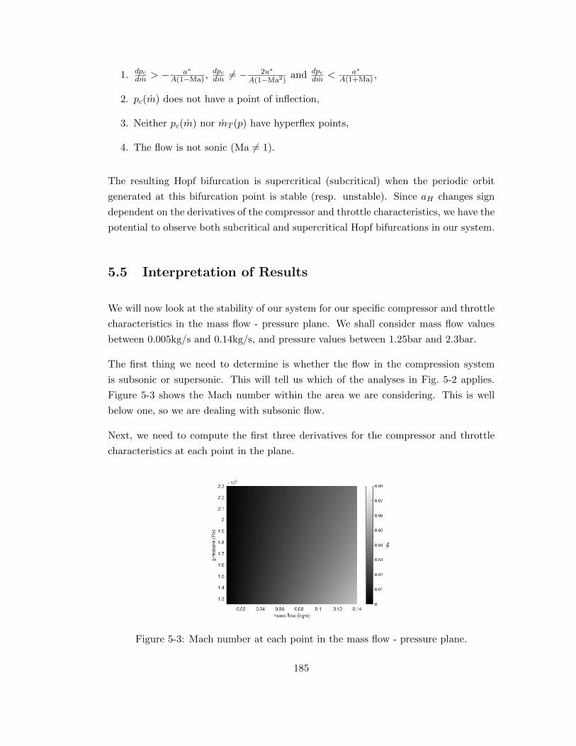
1. dpcdm > − a∗
A(1−Ma) , dpcdm 6= − 2u∗
A(1−Ma2)and dpc
dm < a∗A(1+Ma) ,
2. pc(m) does not have a point of inflection,
3. Neither pc(m) nor mT (p) have hyperflex points,
4. The flow is not sonic (Ma 6= 1).
The resulting Hopf bifurcation is supercritical (subcritical) when the periodic orbit
generated at this bifurcation point is stable (resp. unstable). Since aH changes sign
dependent on the derivatives of the compressor and throttle characteristics, we have the
potential to observe both subcritical and supercritical Hopf bifurcations in our system.
5.5 Interpretation of Results
We will now look at the stability of our system for our specific compressor and throttle
characteristics in the mass flow - pressure plane. We shall consider mass flow values
between 0.005kg/s and 0.14kg/s, and pressure values between 1.25bar and 2.3bar.
The first thing we need to determine is whether the flow in the compression system
is subsonic or supersonic. This will tell us which of the analyses in Fig. 5-2 applies.
Figure 5-3 shows the Mach number within the area we are considering. This is well
below one, so we are dealing with subsonic flow.
Next, we need to compute the first three derivatives for the compressor and throttle
characteristics at each point in the plane.
Figure 5-3: Mach number at each point in the mass flow - pressure plane.
185

Consider the throttle characteristic
m = mT (p, µ) =√σf(µ)(p− pamb). (5.5.1)
We can directly calculate the derivatives of the throttle characteristic for different values
of pressure and throttle parameter, i.e.
∂imT
∂pi(p, µ), for i = 1, 2, 3. (5.5.2)
However, we require the value of the gradient in terms of mass flow and pressure.
Therefore, we have to invert the throttle characteristic to find
µ = m−1T (m, p). (5.5.3)
Similarly, we can numerically compute the derivatives of the compressor characteristic
for different mass flow and impeller speed values, i.e.
∂ipc∂mi
(m,Ω), for i = 1, 2, 3. (5.5.4)
Therefore, we have to compute the inverse
Ω = p−1c (m, p) (5.5.5)
in order to calculate the derivates at points in the mass flow - pressure plane.
Since the inverses of the two characteristics are unknown, we numerically invert them
on a grid in the mass flow - pressure plane. This inversion process is the main source
of numerical error in the following analysis.
Having computed the derivatives, we can now compute detJ∗ and trJ∗ in order to
check the linear stability criteria. Figure 5-4 shows the results. Notice that detJ∗ > 0
everywhere, so we do not observe saddle points.
This also means that trJ∗ is the only function that determines the stability of the
system. Whenever trJ∗ < 0 the system is stable and trJ∗ > 0 the system is unstable.
Therefore, using Eq. 5.3.21 to compute trJ∗ = 0 is a quick way to determine the
location of the surge limit.
Also, since detJ∗ > 0, we know that whenever trJ∗ = 0 we get a Hopf bifurcation. In
186

Figure 5-4: Surface plots of the determinant (left) and trace (right) of the Jacobian inthe mass flow - pressure plane, wherever the gradients of characteristics are defined.
order to determine the form of these bifurcations, we need to compute parameters dH
and aH at the trJ∗ = 0 lines.
The shaded region in Fig. 5-5 shows the area in the mass flow - pressure plane where
dH < 0, and the three black lines identify where trJ∗ = 0. Notice that we do not get
clean lines or edges of the shaded regions because of the numerical error introduced by
inverting the characteristics on a grid. However, starting from high mass flow rates, we
can identify that the first line occurs in the dH < 0 region, the second in dH > 0 and
the third in dH < 0. This means that the middle Hopf bifurcation is in the opposite
direction to the other two.
Figure 5-5: Region (grey) in mass flow - pressure plane where dH < 0. Lines indicatingwhere trJ∗ = 0 are added in black.
187
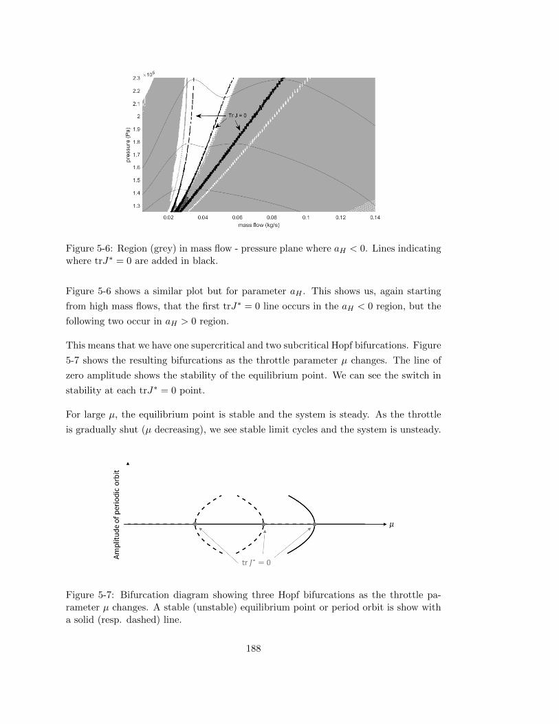
Figure 5-6: Region (grey) in mass flow - pressure plane where aH < 0. Lines indicatingwhere trJ∗ = 0 are added in black.
Figure 5-6 shows a similar plot but for parameter aH . This shows us, again starting
from high mass flows, that the first trJ∗ = 0 line occurs in the aH < 0 region, but the
following two occur in aH > 0 region.
This means that we have one supercritical and two subcritical Hopf bifurcations. Figure
5-7 shows the resulting bifurcations as the throttle parameter µ changes. The line of
zero amplitude shows the stability of the equilibrium point. We can see the switch in
stability at each trJ∗ = 0 point.
For large µ, the equilibrium point is stable and the system is steady. As the throttle
is gradually shut (µ decreasing), we see stable limit cycles and the system is unsteady.
Figure 5-7: Bifurcation diagram showing three Hopf bifurcations as the throttle pa-rameter µ changes. A stable (unstable) equilibrium point or period orbit is show witha solid (resp. dashed) line.
188

Figure 5-8: Suggested global bifurcation diagram for our system based on evidencefrom numerical simulation.
As we reduce µ further, we have unstable limit cycles. We would need to look at a
global picture to fully understand the behaviour of the system at this point.
Figure 5-8 shows an estimate of a global bifurcation diagram. Here we are predicting
saddle node bifurcations from the unstable Hopf bifurcations that result in stable period
orbits.
These stable periodic orbits do not have to grow with the bifurcation parameter µ, so
can explain why deep surge appears to be a fixed amplitude oscillation. Our estimate
for the location of these saddle nodes was deduced by studying Paper 3, Fig. 15 (Section
4.3).
This simulation showed us that we had a region of mild surge, followed by a region
where a combination of mild and deep surge limit cycles were observed. This implies
that a large amplitude periodic orbit (relating to deep surge) could be observed within
the first region where the equilibrium point becomes unstable. It also implies that
there must be a relatively small basin of attraction for both stable periodic orbits as
we can jump between them within a single simulation.
Paper 3, Fig. 15 then showed us that we have region where the simulation is either
stable, or a large amplitude periodic orbit, depending on the initial condition. So
189
again, we must have two stable behaviours. The unstable periodic orbit separates
these two stable behaviours. Since there is a larger distance between the stable and
unstable behaviour, it explains why the system does not jump between these two stable
behaviours within a simulation. It would require a larger deviation between calculated
points than that caused by numerically solving the ODEs or PDEs.
Finally, Paper 3 Fig. 15 observes a region where the only stable behaviour is a large
amplitude periodic orbit corresponding to deep surge. We observe this after the final
(smallest µ) bifurcation point.
Further investigation is needed in order to verify this global bifurcation picture. One
possibility would be to use a numerical continuation software, like AUTO [64].
Another area needing further investigation is the effect of including an inlet pipe into
the system. As seen in Fig. 5-5 or 5-6, the trJ∗ = 0 lines coincide with the turning
points of the compressor characteristic. This location of the surge line agrees with what
we observed in Section 2.5, when we had no inlet pipe. However, in Section 4.3, we
observed that the surge limits were further to the left than this. Therefore, performing
stability analysis on the system of 4 ODEs that take into account the inlet pipe may
produce different criteria for the location of the surge lines.
5.6 Conclusions
In this chapter we analysed the mathematical stability of our reduced order surge model.
We discovered that the operating point of the system is an equilibrium point, and so
the stability of the compression system depends on the stability of that equilibrium.
We performed linear stability analysis and discovered that the gradient of the compres-
sor and throttle characteristics were key factors in determining the stability. We also
noticed that the stability of the system changes dramatically if the flow in the pipework
is supersonic instead of subsonic.
Furthermore, we discovered that Hopf bifurcations exist whenever the trace of our
Jacobian is zero. For our compressor and throttle characteristics, we discovered that
we get three successive Hopf bifurcations: one supercritical and two subcritical.
We proposed a global bifurcation diagram based on our analysis and numerical simu-
lations of our model. This proposes an explanation for the multiple stable phenomena
190
observed in simulations (e.g. a stable equilibrium and stable limit cycle), and suggests
they are separated by an unstable limit cycle generated from a Hopf bifurcation.
A similar analysis was conducted by Hos et al. [28] for a linearised system. In their
work, the Mach number of the fluid did not appear in calculations, meaning the switch
of stability due to sonic flow only occurs due to the nonlinearity in our model.
They obtained a similar stability analysis picture to Fig. 5-2(a), but with the trJ∗ = 0
line entirely in the region of positive compressor gradient. Therefore, using a linearised
system may predict the onset of surge later than observed experimentally for lower
impeller speeds.
Furthermore, they used a cubic polynomial for the compressor characteristic, and this
resulted in one Hopf bifurcation. The stability of the resulting periodic orbit depended
on the parameter for the intercept of the throttle characteristic, which we know relates
to the value of ambient pressure.
For low impeller speeds where we observe a cubic-shaped, rather than quintic-shaped,
characteristic, we observe a single supercritical Hopf bifurcation. This is similar to the
results in Hos et al. [28] for smaller values of their intercept parameter.
Finally, we noted that it would be useful to undertake further work into the global
bifurcations occurring of our model, and on a stability analysis for a model that incor-
porates an inlet pipe.
191

192
Chapter 6
Conclusions
The work undertaken in this thesis was motivated by the problem of identifying surge
limits in radial compressors, with a particular emphasis on automotive turbochargers.
In Chapter 2, we developed a reduced order model for a compression system that in-
cluded a compressor and a throttle valve. We then developed steady-state throttle and
compressor characteristics to be incorporated into the reduced order surge model. All
models were developed using averaging to reduce the dimension of the 3D fundamental
equations of motion.
We also included two more empirical loss functions into the compressor characteristic to
take into account friction and incidence losses. These introduced two parameters into
the model that need universal relations in order for the model to be fully predictive.
In Chapter 3, we looked in more detail at the behaviour of air when it is travelling back-
wards through the compressor. We developed a model for reverse flow that took into
account shear losses at the interface between the impeller and the diffuser. The shear
loss parameter was calibrated by assuming the compressor characteristic is continuous.
During experimental validation of the reversed flow model, the resulting data appeared
to imply the existence of an asymptote near zero mass flow as we approach from m < 0.
However, the surge study carried out in Chapter 4 shows that an asymptote is unlikely
to exist in a characteristic and so this behaviour was more likely caused by a system
level phenomenon.
In Chapter 4, we included a further loss function into the compressor model relating to
diffuser recirculation. This resulted in a new shape of compressor characteristic never
193
derived before in literature. Combining this characteristic with the reduced order
model for surge allowed us to capture both mild and deep surge oscillations, as well as
phenomena like an observed mid-surge quiet period.
We also used the PDE form of the reduced order surge model and solved this numeri-
cally using a staggered grid method. This allowed us to capture wave dynamics in the
compression system pipework.
Furthermore, we modelled a compression system with both an inlet and outlet pipe
in order to compare to experimental data. This gave us insight into the role the inlet
pipe has on the system, including frequency, and stability (when comparing to results
in Chapter 5).
Finally, in Chapter 5, we performed stability analysis on our model to mathematically
determine the location of the surge limit. We discovered that the gradients of the
compressor and throttle characteristics were key for determining stability.
We also discovered that we observe Hopf bifurcations whenever we have a switch in
stability. We obtain both supercritical and subcritical Hopf bifurcations, and have
suggested a global bifurcation diagram that would explain the simulated dynamics
observed from our model.
6.1 Key Insights
Throughout this research project, we have learned many things about the dynamics of
surge and the key physical phenomena involved. We list the key points below.
1. Friction is needed to simulate operation of a radial compressor.
We derived the steady-state compressor characteristic by starting with the sim-
plest possible dynamics, and included additional physical phenomena based on
the results. In the isentropic formulation we discovered that the simulated com-
pressor generated more pressure for higher flow rates, whereas the opposite holds
true in experiments. It was only with the addition of friction that we were able
to simulate realistic behaviour of a compressor.
2. Incidence loss is a key phenomenon for simulating surge.
Similarly to point 1, we observed that a model with friction but no other losses
could not simulate unsteady behaviour reminiscent of surge. With the inclusion
194

of incidence losses, we observed the existence of limit cycles. Once we had the
stall function tending to zero as the flow tends to zero, we were able to relate
these limit cycles to deep surge cycles.
3. Shear losses are important for reverse flow conditions.
We studied flow travelling in the reverse direction through a radial compressor.
We noticed that there is a large jump in tangential velocity at the impeller -
diffuser interface that would cause losses. This explained why we were observing
higher than expected pressure values at small negative mass flow rates. By in-
cluding this loss, we were able to regain a continuous compressor characteristic
that could simulate deep surge cycles.
4. Diffuser recirculation is vital for observing mild surge.
We noticed that for high impeller rotational speeds, we were not capturing the
location of surge onset as well as for lower speeds. This prompted us to add
diffuser recirculation into the steady-state compressor characteristic model. We
used the same form of the stall function as with incidence losses, and this resulted
in a characteristic with two local minima, instead of just one. Having this extra
minima allowed our reduced order surge model to simulate two different limit
cycles, and we related each cycle to mild or deep surge depending on the amplitude
of oscillation. This was the first time any model had been able to capture and
explain the existence of both mild and deep surge.
5. Mid-surge quiet period is explained by interaction between the two types of stall.
We observed that our model simulated a region of stable operation after mild
surge had been triggered but prior to a deep surge cycle. This area typically
coincided with a region of negative gradient for the compressor characteristic.
This negative gradient is caused by the interaction between impeller inlet stall
(caused by incidence losses) and diffuser stall (caused by local flow recirculation).
Diffuser stall is triggered first and causes a pressure drop. When impeller stall
was triggered, this straightened the flow entering the diffuser and so reduced
the pressure drop caused by diffuser stall. This recovery of pressure causes the
negative gradient in that region of the compressor characteristic.
6. Stability is dependent on Mach number and gradients of characteristic curves.
We performed mathematical stability analysis on the reduced order surge model.
Using the fact that the operating point of the system is an equilibrium, we calcu-
lated the Jacobian matrix at this point to understand the linear stability of the
system. By considering the determinant and trace of the Jacobian, we were able
195
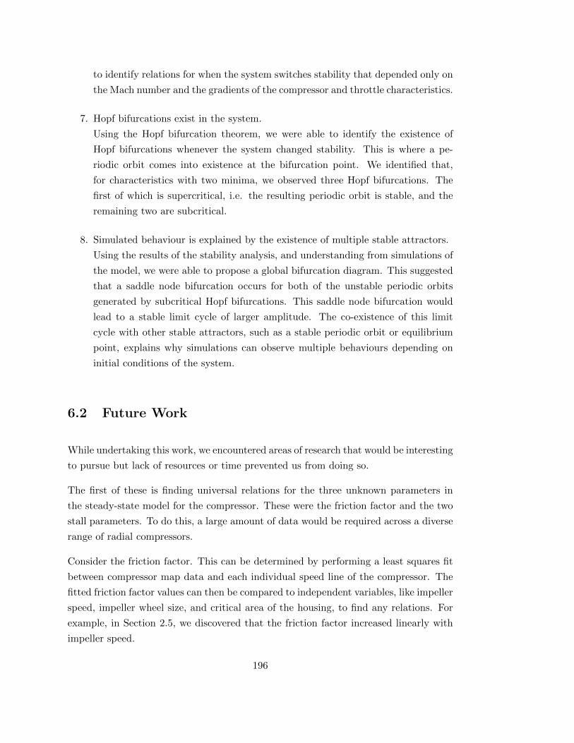
to identify relations for when the system switches stability that depended only on
the Mach number and the gradients of the compressor and throttle characteristics.
7. Hopf bifurcations exist in the system.
Using the Hopf bifurcation theorem, we were able to identify the existence of
Hopf bifurcations whenever the system changed stability. This is where a pe-
riodic orbit comes into existence at the bifurcation point. We identified that,
for characteristics with two minima, we observed three Hopf bifurcations. The
first of which is supercritical, i.e. the resulting periodic orbit is stable, and the
remaining two are subcritical.
8. Simulated behaviour is explained by the existence of multiple stable attractors.
Using the results of the stability analysis, and understanding from simulations of
the model, we were able to propose a global bifurcation diagram. This suggested
that a saddle node bifurcation occurs for both of the unstable periodic orbits
generated by subcritical Hopf bifurcations. This saddle node bifurcation would
lead to a stable limit cycle of larger amplitude. The co-existence of this limit
cycle with other stable attractors, such as a stable periodic orbit or equilibrium
point, explains why simulations can observe multiple behaviours depending on
initial conditions of the system.
6.2 Future Work
While undertaking this work, we encountered areas of research that would be interesting
to pursue but lack of resources or time prevented us from doing so.
The first of these is finding universal relations for the three unknown parameters in
the steady-state model for the compressor. These were the friction factor and the two
stall parameters. To do this, a large amount of data would be required across a diverse
range of radial compressors.
Consider the friction factor. This can be determined by performing a least squares fit
between compressor map data and each individual speed line of the compressor. The
fitted friction factor values can then be compared to independent variables, like impeller
speed, impeller wheel size, and critical area of the housing, to find any relations. For
example, in Section 2.5, we discovered that the friction factor increased linearly with
impeller speed.
196

Using statistical regression, like the Generalised Additive Model approach described in
Section 1.2.2, we can formalise this and find relations for parameters in cases where
the interactions between independent variables are important.
The second area to explore is the form of the stall functions used for impeller incidence
and diffuser recirculation. In Section 2.6.1 we had a free choice of the parameter d
provided it was non-zero. Therefore, exploring different possibilities for d, and its effect
on the resulting compressor characteristic and surge dynamics, would be interesting and
may allow us to capture the surge limit to higher accuracy.
Moreover, in Section 4.3 the fitted value for the diffuser stall parameter was not constant
and did not appear to have a relationship to independent variables (like impeller speed)
that could be explained physically. It would be useful to explore the form of the stall
function in this case because it is possible that it is not capturing the physical dynamics
of diffuser recirculation. For example, we identified that the critical angle at which local
flow reversal occurs, α∗, may need a model itself as it is a complex phenomena that
could depend on many factors of the flow.
The final area to explore in relation to the compressor characteristic is the effect of
inlet pressure. As discovered in Section 4.5, changing the inlet pressure appears to
cause a simple shift and stretch of the characteristics at ambient pressure. Formally
deriving this relation would help us understand exactly how the inlet pipe influences
the compressor system.
Furthermore, knowing the exact form of this relation would help us to incorporate the
effect of the inlet pipe into the stability analysis conducted in Chapter 5. For example,
if we understand how the inlet pressure varies with mass flow, and know the effect this
has on the compressor characteristic, we could use
dpcdm
(m, p0) =∂pc∂m
+∂pc∂p0
dp0
dm(6.2.1)
in the derived formulae to understand the effect inlet pressure has on the location of
the surge line.
There are other ways in which we could incorporate the effect of the inlet pipe into
the dynamical systems theory and stability analysis performed in Chapter 5. One way
would be to analyse the 4D system found by the PDE form of the reduced order surge
model with N=4 (see Section 4.1). This would result in a 4x4 matrix for the Jacobian,
and therefore make the analytical formulae far more complex and difficult to derive. It
197

is likely that numerical computation would be the most efficient way forward in this
case.
Another approach is to perform dynamical systems analysis on a discrete-time map.
Consider the linearised PDEs for flow in a pipe,
∂p
∂t+a2
A
∂m
∂x= 0, (6.2.2)
∂m
∂t+A
∂p
∂x= 0. (6.2.3)
If we change variables to
v+ = p+a
Am, (6.2.4)
v− = p− a
Am (6.2.5)
then
dv+
dt(x, t) = 0 on
dx
dt= a, (6.2.6)
dv−dt
(x, t) = 0 ondx
dt= −a. (6.2.7)
This means that a map can be found for the pressure and mass flow at different locations
in the pipe. Fig. 6-1 shows how this works for the pressure at the midpoint of the outlet
pipe. Here the difference in time between pn and pn+1 is L2a .
The boundary conditions allow the inclusion of the effects of the inlet pipe, and the
fact we have no averaging over the length of the pipe means wave dynamics will still
occur in this system.
Another area to explore is the behaviour of the reversed-flow tests at low mass flow
rates (see Section 3.2). The results from the experiments seemed to suggest that the
compressor characteristic had an asymptote near zero flow for high impeller speeds.
However, the surge tests for the same compressor (conducted in Section 4.3) imply
that this asymptotic behaviour is more likely due to a system level phenomenon.
It would be very interesting to repeat the reverse flow tests with the focus of under-
standing this behaviour. It would also be interesting if the behaviour could be captured
by modelling the reverse flow experimental procedure in a similar manner to our PDE
form of the surge model in Section 4.3. A new form of the throttle characteristic would
probably have to be developed in order to capture the true behaviour of high pressure
198
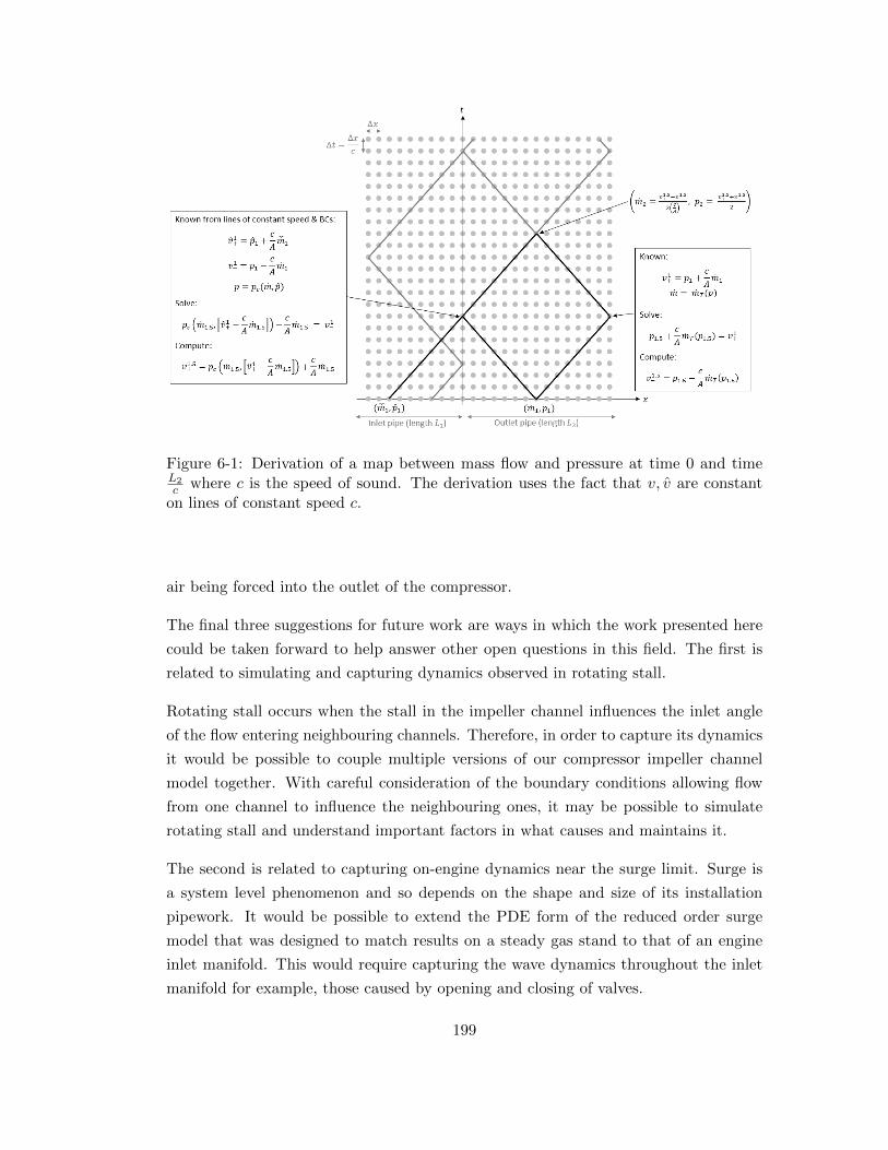
Figure 6-1: Derivation of a map between mass flow and pressure at time 0 and timeL2c where c is the speed of sound. The derivation uses the fact that v, v are constant
on lines of constant speed c.
air being forced into the outlet of the compressor.
The final three suggestions for future work are ways in which the work presented here
could be taken forward to help answer other open questions in this field. The first is
related to simulating and capturing dynamics observed in rotating stall.
Rotating stall occurs when the stall in the impeller channel influences the inlet angle
of the flow entering neighbouring channels. Therefore, in order to capture its dynamics
it would be possible to couple multiple versions of our compressor impeller channel
model together. With careful consideration of the boundary conditions allowing flow
from one channel to influence the neighbouring ones, it may be possible to simulate
rotating stall and understand important factors in what causes and maintains it.
The second is related to capturing on-engine dynamics near the surge limit. Surge is
a system level phenomenon and so depends on the shape and size of its installation
pipework. It would be possible to extend the PDE form of the reduced order surge
model that was designed to match results on a steady gas stand to that of an engine
inlet manifold. This would require capturing the wave dynamics throughout the inlet
manifold for example, those caused by opening and closing of valves.
199

In doing this, it might be possible to predict the surge limit for specific on-engine
applications. This would remove the need for an estimated surge margin on compressor
maps which takes into account the uncertainty of how a compressor will operate when
installed for a particular application, rather than the gas stand there the map was
initially generated.
The last is looking into a way to control or mitigate surge behaviour. Once a global
bifurcation analysis has been performed, it would be possible to identify domains of
attraction of stable behaviour and use this insight to design control strategies. These
strategies are likely to involve mechanisms for flow management that could prevent or
quickly respond to the existence of surge-like behaviour in a system.
200

References
[1] N. Watson and M. S. Janota, Turbocharging: The internal combustion engine. MacMillan,1982.
[2] R. Stone, Introduction to internal combustion engines. Palgrave MacMillan, 4 ed., 2012.
[3] “Turbocharger history.” http://www.cummins.ru/en/components/
turbo-technologies/turbocharger-history. [Online], Accessed 07/12/2020.
[4] “Turbocharger history.” http://www.turbo-tec.eu/uk/turbocharger-history/. [On-line], Accessed 07/12/2020.
[5] “Axial compressors.” http://turbomachinery.mandieselturbo.com/products/
compressors/axial. [Online], Accessed 19/01/2018.
[6] “Turbocharger.” https://en.wikipedia.org/wiki/Turbocharger. [Online], Accessed03/08/2016.
[7] “Axial compressor.” https://en.wikipedia.org/wiki/Axial_compressor. [Online], Ac-cessed 19/01/2018.
[8] “Centrifugal compressor.” https://en.wikipedia.org/wiki/Centrifugal_compressor.[Online], Accessed 03/08/2016.
[9] T. Puiu, “This is what 109,000 horsepower looks like.” https://www.zmescience.com/
science/biggest-most-poweful-engine-world/, 2019. [Online], Accessed 07/12/2020.
[10] “Broadest turbo range.” https://www.garrettmotion.com/turbocharger-technology/
how-a-turbo-works/broadest-turbo-range/. [Online], Accessed 07/12/2020.
[11] “Turbocharger specs.” https://turbochargerspecs.blogspot.com/2013/03/
garrett-gt06-gt0632sz-32-trim-80-hp.html, 2013. [Online], Accessed 07/12/2020.
[12] “History.” http://www.turbos.bwauto.com/en/products/turbochargerHistory.
aspx#:~:text=The%20real%20breakthrough%20in%20passenger,VW%20Golf%
20Turbodiesel%20in%201981. [Online], Accessed 07/12/2020.
[13] D. for Transport, “Vehicle licensing statistics: 2019 quar-ter 1 (jan-mar).” https://assets.publishing.service.gov.uk/
government/uploads/system/uploads/attachment_data/file/812253/
vehicle-licensing-statistics-january-to-march-2019.pdf. [Online], Accessed07/12/2020.
[14] “Synthetic fuels/audi e-fuels.” https://www.audi-mediacenter.com/en/
audi-e-fuels-243. [Online], Accessed 07/12/2020.
[15] B. Roy and A. M. Pradeep, “Turbomachinery aerodynamics.” http://nptel.ac.in/
courses/101101058/downloads/Lec-31ppts.pdf. [Online], Accessed 03/08/2016.
201

[16] M. Stewart, Surface Production Operations. Gulf Professional Publishing, Boston, 2019.
[17] E. M. Greitzer, “Surge and rotating stall in axial flow compressors - Part I: Theoreticalcompression system model,” Journal of Engineering for Power, vol. 98, no. 2, pp. 190–198,1976.
[18] D. A. Fink, Surge Dynamics and Unsteady Flow in Centrifugal Compressors. PhD thesis,Massachusetts Institute of Technology, 1988.
[19] D. A. Fink, N. A. Cumpsty, and E. M. Greitzer, “Surge dynamics in a free-spool centrifugalcompressor system,” Journal of Turbomachinery, vol. 114, pp. 321– 332, 1992.
[20] R. L. Elder and M. E. Gill, “A discussion of the factors affecting surge in centrifugalcompressors,” Journal of Engineering for Gas Turbines and Power, vol. 107, pp. 499–506,1985.
[21] K. Chan, A. Ordys, K. Volkov, and O. Duran, “Comparison of engine simulation softwarefor development of control system,” Modelling and Simulation in Engineering, vol. 2013,2013.
[22] I. Gamma Technologies, “Gt-power engine simulation software.” https:
//www.gtisoft.com/gt-suite-applications/propulsion-systems/
gt-power-engine-simulation-software/. [Online], Accessed 17/01/2021.
[23] O. Vıtek, J. Macek, and M. Polasek, “New approach to turbocharger optimization using1-d simulation tools,” tech. rep., SAE Technical Paper, 2006.
[24] I. Gamma Technologies, “Gt-suite engine performance tutorials.” https:
//mycourses.aalto.fi/pluginfile.php/637426/mod_folder/content/0/Engine_
Performance-tutorials.pdf. [Online], Accessed 17/01/2021.
[25] A. Rose, Application of a Continuously Variable Transmission to Engine Boosting andExhaust Energy Recovery Systems. PhD thesis, University of Bath, 2013.
[26] I. Day, “Stall, surge, and 75 years of research,” Journal of Turbomachinery, vol. 138, no. 1,p. 011001, 2016.
[27] G. L. Arnulfi, P. Giannattasio, C. Giusto, A. F. Massardo, D. Micheli, and P. Pina-monti, “Multistage centrifugal compressor surge analysis: Part II - Numerical simulationand dynamic control parameters evaluation,” Journal of Turbomachinery, vol. 121, no. 2,pp. 312–320, 1999.
[28] C. Hos, A. Champneys, and L. Kullmann, “Bifurcation analysis of surge and rotatingstall in the Moore–Greitzer compression system,” IMA Journal of Applied Mathematics,vol. 68, no. 2, pp. 205–228, 2003.
[29] H. Tamaki, “Effect of piping systems on surge in centrifugal compressors,” Journal ofMechanical Science and Technology, vol. 22, no. 10, pp. 1857–1863, 2008.
[30] S. G. Koff and E. M. Greitzer, “Stalled flow performance for axial compressors: I - Axisym-metric characteristic,” in 29th International Gas Turbine Conference and Exhibit, vol. 1,American Society of Mechanical Engineers, 1984.
[31] J. Galindo, J. Serrano, H. Climent, and A. Tiseira, “Experiments and modelling of surgein small centrifugal compressor for automotive engines,” Experimental Thermal and FluidScience, vol. 32, no. 3, pp. 818–826, 2008.
[32] F. K. Moore and E. M. Greitzer, “A theory of post-stall transients in axial compressionsystems: Part I - Development of equations,” Journal of Engineering for Gas Turbinesand Power, vol. 108, no. 1, pp. 68–76, 1986.
202
[33] M. Zagorowska and N. Thornhill, “Compressor map approximation using chebyshev poly-nomials,” 2017.
[34] X. Li, C. Yang, Y. Wang, and H. Wang, “A prediction model of compressor with variable-geometry diffuser based on elliptic equation and partial least squares,” Royal Society openscience, vol. 5, no. 1, p. 171468, 2018.
[35] G. Martin, V. Talon, P. Higelin, A. Charlet, and C. Caillol, “Implementing turbomachineryphysics into data map-based turbocharger models,” SAE International Journal of Engines,vol. 2, no. 1, pp. 211–229, 2009.
[36] D. Japikse, Centrifugal compressor design and performance, vol. 2. Concepts Eti WhiteRiver Junction, VT, 1996.
[37] E. I. G. VELaSQUEZ, “Determination of a suitable set of loss models for centrifugal com-pressor performance prediction,” Chinese Journal of Aeronautics, vol. 30, no. 5, pp. 1644–1650, 2017.
[38] H. W. Oh, E. S. Yoon, and M. Chung, “An optimum set of loss models for performanceprediction of centrifugal compressors,” Proceedings of the Institution of Mechanical Engi-neers, Part A: Journal of Power and Energy, vol. 211, no. 4, pp. 331–338, 1997.
[39] X. Gong and R. Chen, “Total pressure loss mechanism of centrifugal compressors,” Me-chanical engineering research, vol. 4, no. 2, p. 45, 2014.
[40] K. W. Linfield and R. G. Mudry, “Pros and cons of cfd and physical flow modeling,”Airflow Sciences Corporation, 2008.
[41] P. Fischer, “Introduction to galerkin methods.” http://fischerp.cs.illinois.edu/
tam470/refs/galerkin2.pdf. [Online], Accessed 22/12/2020.
[42] J. Ratz, S. Leichtfuß, M. Beck, H.-P. Schiffer, and F. Frohlig, “Surge margin optimizationof centrifugal compressors using a new objective function based on local flow parameters,”International Journal of Turbomachinery, Propulsion and Power, vol. 4, no. 4, p. 42, 2019.
[43] A. D. Muradova, “The spectral method and numerical continuation algorithm for the vonkarman problem with postbuckling behaviour of solutions,” Advances in ComputationalMathematics, vol. 29, no. 2, pp. 179–206, 2008.
[44] I. Lomtev and G. E. Karniadakis, “A discontinuous galerkin method for the navier–stokesequations,” International journal for numerical methods in fluids, vol. 29, no. 5, pp. 587–603, 1999.
[45] S. N. Wood, Generalized additive models: an introduction with R. CRC press, 2017.
[46] J. A. Sanders, F. Verhulst, and J. Murdock, Averaging methods in nonlinear dynamicalsystems, vol. 59. Springer, 2007.
[47] H. Steinruck, Asymptotic methods in fluid mechanics: Survey and recent advances, vol. 523.Springer Science & Business Media, 2012.
[48] J. Hateley, “The lorenz system.” http://web.math.ucsb.edu/~jhateley/paper/
lorenz.pdf. [Online], Accessed 17/01/2021.
[49] D. John and J. Anderson, “Computational fluid dynamics: the basics with applications,”P. Perback, International ed., Published, 1995.
[50] “B5.4 waves & compressible flow.” https://www0.maths.ox.ac.uk/system/files/
coursematerial/2015/3080/19/wcf.pdf. [Online], Accessed 19/07/2016.
203
[51] D. J. Acheson, Elementary fluid dynamics. Oxford University Press, 1990.
[52] R. Von Mises, H. Geiringer, and G. S. S. Ludford, Mathematical theory of compressiblefluid flow. Courier Corporation, 1958.
[53] E. M. Greitzer, C. S. Tan, and M. B. Graf, Internal flow: concepts and applications.Cambridge University Press, 2004.
[54] P. R. N. Childs, Rotating Flow. Elsevier Inc., 2011.
[55] H. Stewart, “The energy equation for a viscous compressible fluid,” Proceedings of theNational Academy of Sciences, vol. 28, pp. 161–164, 1942.
[56] K. P. Burr, T. R. Akylas, and C. C. Mei, “Chapter 2: Two-dimensional laminarboundary layers.” http://web.mit.edu/fluids-modules/www/highspeed_flows/ver2/
bl_Chap2.pdf. [Online], Accessed 27/03/2017.
[57] D. E. Winterbone and R. J. Pearson, Theory of engine manifold design: Wave actionmethods for IC engines. Professional Engineering Publishing, 2000.
[58] C. W. Gear and O. Osterby, “Solving ordinary differential equations with discontinuities,”ACM Transactions on Mathematical Software (TOMS), vol. 10, no. 1, pp. 23–44, 1984.
[59] A. V. Wouwer, P. Saucez, and C. Vilas, Simulation of Ode/Pde Models with MATLAB®,OCTAVE and SCILAB: Scientific and Engineering Applications. Springer, 2014.
[60] S. Wiggins, Introduction to applied nonlinear dynamical systems and chaos, vol. 2. SpringerScience & Business Media, 2003.
[61] G. Layek, An introduction to dynamical systems and chaos. Springer, 2015.
[62] “Stability theory.” https://en.wikipedia.org/wiki/Stability_theory. [Online], Ac-cessed 03/02/2021.
[63] J. Guckenheimer and P. Holmes, Nonlinear oscillations, dynamical systems, and bifurca-tions of vector fields, vol. 42. Springer Science & Business Media, 2013.
[64] “Auto software for continuation and bifurcation problems in ordinary differential equa-tions.” http://cmvl.cs.concordia.ca/auto/. [Online], Accessed 17/02/2021.
204