NASA Technical Memorandum 108863 USAATCOM Technical Report 94-A-022i'

/

d "

" 49"

Development and Validation ofa Blade-Element Mathematical Model

for the AH-64A Apache Helicopter

M. Hossein Mansur

(NASA-TM-108863) DEVELCPMENT AND

VALIOATION OF A BLADE-ELEMENT

MATHEMATICAL MODEL FOR THE AH-64A

APACHE HELICOPTER (Army Aviation

Systems Command) 98 p

N95-26710

Unclas

G3/OI 0048163

April 1995

National Aeronautics andSpace Administration

VUS ArmyAviation and Troop Command

Aeroflightdynamics DirectorateMoffett Field, CA 94035-1000

https://ntrs.nasa.gov/search.jsp?R=19950020290 2018-06-04T21:28:01+00:00Z

NASA Technical Memorandum 108863 USAATCOM Technical Report 94-A-022

Development and Validation ofa Blade-Element Mathematical Model

for the AH-64A Apache Helicopter

M. Hossein Mansur, Aeroflightdynamics Directorate, U.S. Army Aviation and Troop

Command, Ames Research Center, Moffett Field, California

April 1995

National Aeronautics and

Space Administration

Ames Research Center

Moffett Field, CA 94035-1000

US ArmyAviation and Troop Command

Aeroflightdynamics DirectorateMoffett Field, CA 94035-1000

Development and Validation of a Blade-Element

Mathematical Model for the AH-64A Apache

Helicopter

M. Hossein Mansur

Aeroflightdynamics Directorate

U.S. Army Aviation and Troop CommandAmes Research Center

Summary

A high-fidelity blade-element mathematical model for the AH-64A Apache Advanced Attack

Helicopter has been developed by the Aeroflightdynamics Directorate of the U.S. Army's Aviation and

Troop Command (ATCOM) at Ames Research Center. The model is based on the McDonnell Douglas

Helicopter Systems' (MDHS) Fly Real Time (FLYRT) model of the AH-64A (acquired under contract)

which was modified in-house and augmented with a blade-element-type main-rotor module. This report

describes, in detail, the development of the rotor module, and presents some results of an extensive

validation effort.

Introduction

High-fidelity simulation models of helicopters are needed for a variety of tasks including han-

dling qualities evaluations, pilot training, simulation of life-cycle upgrades, and accident investigations.

Many different approaches are currently used to develop mathematical models for helicopters. These

approaches can be organized into three distinct categories (ref. 1): 1) analytical models, 2) identified

models, and 3) combinations of 1 and 2. Analytical models rely on dynamic and aerodynamic theoriesand usually attempt to model each component of the helicopter individually. The combined, end-to-

end, responses of such models are generally accurate for the dominant responses and nonlinearities, but

are often imprecise in modeling rotor dynamics, especially in the off-axis (ref. 2). Identified models,

on the other hand, use available vehicle-response data (collected through flight testing) to generate

models which accurately characterize the end-to-end responses of an existing aircraft. Such models are

commonly used during prototype testing for optimization of flight control systems, where very accurate

response prediction is critical. In addition, they are very useful bases for simulation model validation,

as is demonstrated herein. Identified models generally do not attempt to treat the components of

the helicopter individually and their region of validity is restricted to the configuration and the linear

response at the flight condition of the identification. Further, there is no way to identify models of

aircraft still under development (prior to first flight) since there can be no access to flight-test data forsuch vehicles.

Component type models are, therefore, the only way to simulate helicopters during the design

phase, and provide the best way to simulate aircraft over their entire flight envelope. The latter is

especiallytrue at extremeconditions,suchasmay beencounteredin accidentinvestigations.Asidefromtheir applicabilityto theentireflightenvelope,however,thereisafurtheradvantageto makingtheinvestmentof time and resourcesneededto developa componenttypemodelof anexistinghelicopter.This advantageis the availabilityof flight-testdata,whichallowsengineersto performthe extensivetestingandcomparisonsofsimulationandaircraft responsesthat arenecessaryto developnewmodelingmethodsor enhanceexistingones.Theseneworenhancedmethodscanthenbeappliedto themodelingof bothexistingand futurehelicopters,improvingour modelingcapabilityoverall.

In the late 1980sthe U.S.Army initiated effortsto obtain a high-fidelitycomponenttype modelfor the AH-64A Apachehelicopter(fig. 1). The effortwaspromptedby the successof two pilot-in-the-loopUH-60accident-investigation-simulationsconductedat NASAAmes.Thosesimulationswereconductedusingacomponent-typemodelof the BlackHawkknownasGenHel,developedby Sikorskyandexpanded/improvedat Ames(ref.3). A modelwithcomparablecomplexityandfidelitywassoughtfor the AH-64A.

As a result of a competitiveprocurementeffort, the bestavailablemodelfor the AH-64A,the Mc-DonnellDouglasHelicopterSystems'(MDHS)Fly RealTime(FLYRT) (ref.4),wasobtainedincludingvalidation-flight-datain hoverandforwardflight. FLYRTreponseswereshownto matchthe providedflight datareasonablywell. However,a greatshortcomingofFLYRTwasperceivedto beits mMn-rotormodulewhich is basedon a map-typeapproach.This modelingapproachwasoriginMly conceivedinthe late 70sto allow real-timeoperationwith the limited computationalcapabilitiesavailableat thattime (ref.5). Theapproachreliesonapregeneratedmapto determinethe rotor'squasi-steadyresponseat eachcycle.First-order-lagapproximationsto rotor dynamicsarethenaddedto thesequasi-steadyvaluesto completetherotor response.Theproblemwith this techniqueis oneof completedependencyonandrestrictionby this pregeneratedmap,especiMlysincethecodefor the generationof moremapswasnot providedaspart of FLYRT.Therestrictionwasdeemedsurmountablesincethe computationalpowerof current computersmakesit possibleto run blade-elementmodelsin real-time,without theneedfor the generationof a map.

A blade-element-typemain-rotormodulewasthereforedevelopedto replacethe map-typemodulein FLYRT.The goalwasto achievethe flexibility that a blade-element-typemodule,unburdenedbythe restrictionsof a pregeneratedmap,wouldprovide.Further,the accessthat a blade-element-typerotor moduleallowsto the actualphysicalparametersof therotor wouldmakeit possibleto introducecorrections,enhancements,and newtheoriesasthey aredeveloped.It would thereforeallow for con-tinual improvement,which wouldnot havebeenpossiblewith the map-typerotor module.The newrotor wasincorporatedinto FLYRT,alongwith additionalmodificationsasnecessary.Thenewmodelis knownastheBlade-ElementModelfor APache(BEMAP).BEMAP hasbeenvalidatedin compar-isonwith availableflight data in hoverand forwardflight in both time and frequencydomains.Thefrequency-domainvalidationmethodsdrawheavilyon thetoolscontainedin CIFERR (ComprehensiveIdentificationfrom FrEquencyResponses)(ref.6),aswill bediscussed.This reportdescribes,in detail,the derivationof the rotor equationsfor theblade-elementrotor module.It alsopresentssomeresultsfrom the validationeffort. In everycase,FLYRT responseshavebeenincludedfor comparison.Note,however,that the intent is not to showsuperiorityof onemodelto the otherbut to showthat theblade-elementrotor modulehasbeenderivedand implementedcorrectly.

Mathematical Model Description

Tofacilitatethe introductionoftheblade-elementrotor module,FLYRTwasfirst extensivelymodi-fied.Themodificationsincluded:1)reorganizationof thecodeto improvemodularity,2) improvementsin its input/output capability,and3) additionof a plottingcapabilitynot providedunderthe contract.The basicstructureof the new rotor moduleis basedon the main-rotormoduleof GenHel(ref. 7),with the relevantequationsfor modelingthe AH-64Aderivedwith the aid of the symbolicmanipula-tion programMACSYMA (ref.8). The derivationof the rotor equationswaspart of anearliereffort,initiated by Chen(ref. 9), to developcompletebladedynamicequationsfor fully articulatedconfigu-rationswhichuseoneof thethreehingearrangementsmostcommonlyused,i,e.,lag-flap-pitch(1-f-p),flap-lag-pitch(f-l-p), andflap-pitch-lag(f-p-l). Chenderivedtheinertial portionof theequationsusingaLagrangianapproach,makingnohighorderorsmallangleassumptions.MACSYMAwaslaterusedto rederivethesameequationsusinga Newtonianapproach,againmakingnohighorderor smallangleassumptions.The two setsof equationswerecomparedandwerefound to be in generalagreement.Thoughthe Apacheusesan f-p-1hingesequence,the simplerf-l-p sequencewasusedin the newrotormodule.The choicewasmadein orderto avoidthe addedcomplexitythat wouldhaveresultedfromtreating bladepitch asa degreeof freedom.The reasoningwasthat giventhe small lead-lagangles,the increasedaccuracyachievedby usingthe actualf-p-1sequencewouldbeminimal.

The new rotor was then integratedinto FLYRT to createBEMAP. This alsorequiredthe re-placementof the trim moduleand the modificationof the equations-of-motion(EOFM) module,aswill be discussedlater. The modulesrepresentingothercomponentsof the Apachehelicopter,i.e.,fuselage/empennage/wings,vertical tail/tail rotor, horizontalstabilator,andlandinggearswereuseddirectlyfrom FLYRTwith minimalchangesrequiredforimplementation.TheDigital AutomaticStabi-lizationEquipment(DASE)modelusedin FLYRTwasalsoretained,however,extensivemodificationsto allowintroductionof controlinputsfrom flight-dataweremade.BEMAP is, therefore,a versionofFLYRTwhichhasbeen:1) equippedwith a blade-elementmain-rotormodule,2) upgradedwith newtrim and modifiedequations-of-motionmodules,3) restructuredto improvemodularity,4) enhancedwith flight-data-control-inputaccesscapability for flight-datacomparisons,and 5) updatedwith aversatileplotting option.

The developmentof the newblade-elementmodelwill bediscussedin detail in the next section.Thetrim moduleandthemodificationsto theequations-of-motionmodulewill alsobebrieflydiscussedsubsequently.No attempt is madein this report,however,to redocumentthe moduleswhichremainfunctionallyunchangedor only slightly changedfromFLYRT.The descriptionanddocumentationofthosemodulescan be found in reference4, generatedby MDHS aspart of the contract to deliverFLYRT to theArmy.

Development of the Rotor Module

In order to minimizethe developmenttime of the blade-elementmain-rotormodule,the main-rotor moduleof Sikorsky/AmesGenHelwasusedasa basicstructure.To developanAH-64Aversionof this rotor, it wasnecessaryto: 1) modify the moduleto allow noncollocatedflap and lead-laghinges,2) replaceall UH-60-specificdatawith AH-64A-specificdata,3) incorporatenewaerodynamiccoefficienttablesand new table-lookupand interpolationroutines,and 4) replaceall UH-60-specificequationswith AH-64A-specificequivalents.

Likethe GenHelmain-rotor(ref.3), theBEMAP rotorconsidersflapping,lead-lag,rotor rotationalspeed,and inflow degreesof freedom.An equal-annulimethod(ref. 7), modifiedfor noncollocatedhinges,was implementedto divide eachbladeinto elements.Equationsfor the local velocity andaccelerationof eachelementwerethenderivedbasedon aircraft and blade (lead-lag,flapping,androtational)motionsandtheelement'spositionwith respectto theaircraft Centerof Gravity (C.G.).

Thelocalvelocity,alongwith localinflowandwind,determinethelocalangleof attack andMachnumberfor entry into the aerodynamiccoefficienttables. Thecoefficientsarethen usedto calculatecomponentsof the aerodynamicforceand momentper bladeelement. Summingtheseover all theblade-elementsresultsin the aerodynamicforcesand momentsper blade. No dynamictwisting orbendingof the bladesweremodeled.Thepreformedlineartwist of the blades,however,is representedthroughadjustmentsof the blade-elementpitchangle.

Thelocalaccelerationat the bladeelementwasusedto deriveequationsfor the inertial forcesandmomentsper blade. Unlike the caseof aerodynamicforces,the bladeelementsusedfor the inertialderivationsweredifferentialelementsandanalyticalintegration,ratherthannumericalsummation,wasusedalongthe bladespan.Nosimplifyingassumptionsweremadein the derivationof the equations(asidefrom the assumptionof rigid blades)and, therefore,the equationsare quite complex. They,however,providea goodtool for exploringthe effectsof higherorderterms(usuallydropped)on thefidelity of therotor module.

The derivationof the equationsfor the rotor forces,rotor moments,and the coupledflappingand lead-lagequationsof motion areprovidedin the followingsubsectionsand appendixA. SimpleMACSYMAmacrosdevelopedto aidin the derivationshavealsobeenprovided(app.B). Theaerody-namicportion of the equationsfollowthe methodsusedin the GenHelmain rotor (ref. 7), modifyingfor the AH-64A as necessary.Followingthe GenHelstructure,the BEMAP rotor modulecontainsits own integrationalgorithmwhichgivesflappingand laggingpositionsandvelocitiesin the rotatingframe. TheAH-64A specificdataandthe aerodynamic-coefficienttableswereobtainedfrom the "AirVehicleTechnicalDescriptionData for the AH-64AAdvancedAttack Helicopter,"reference10. Foranglesof attack between-5 degand+30 deg the values of section lift and drag coefficients are from

wind-tunnel tests and are functions of local angle of attack and Mach number. For angles of attack from

+30 deg to +355 deg the values of section lift and drag coefficients are from C-81 equations (ref. 11),are independent of Mach number, and the lift coefficient data include the increase in maximum lift due

to dynamic stall.

The inflow components are calculated using the Pitt/Peters inflow model implemented as described

by Peters and HaQuang in their AHS Technical Note (ref. 12). The model, which is based on unsteady

actuator-disk theory, is valid for forward flight as well as hover and uses coefficients of aerodynamic

thrust, pitching moment, and rolling moment to calculate the three induced velocity states.

Derivation of Rotor Equations

As mentioned previously, the symbolic manipulation program MACSYMA was used to derive the

rotor equations using a Newtonian approach. Figure 2(a) shows the coordinate systems used in the

derivations. As can be seen, the model assumes a fully articulated rotor hub using flapping and lead-lag

hinges in a flap-lag-pitch hinge arrangement, the flapping hinge being closest to the center of rotation.

From the rotor shaft up, the rotating-shaft (rs) frame has its origin at the rotor hub and its y-axis

alongthe bladesegmentbetweenthehubandtheflappinghingeandrotating with the rotor. Frame3is similar to the rotating-shaftsystemexceptthat its origin is at the flappinghinge.Frame2 alsohasits origin at the flappinghingebut hasits y-axisalongthe blade-segmentbetweenthe flappingandthe lead-laghinges,i.e., rotatedaboutthe negativex-axisthrough/3(flappingup ispositive). Finally,frame1 is similar to frame2 exceptthat its origin is locatedon the lead-laghinge.

Velocity and acceleration vectors at the rotor hub- Thetranslationalandrotationalvelocityandaccelerationvectorsat the main-rotorhubdueto themotionof the helicopterareindependentofthe hingesequenceusedfor the rotor. Thesevectorsaretheresultof the translationalandrotationalvelocityandaccelerationof theaircraft'sC.G.andits separationfromtherotorhub (referto fig. 2(b)).

Let:

Vcgb = v = Inertial translational velocity of aircraft C.G. (body axes)w

/ }Wcgb = q = Inertial rotational velocity of aircraft C.G. (body axes)r

_hb = Yh = Hub location relative to C.G. (body axes)

Zh

The translational velocity at the rotor hub, in body axes, may then be calculated from:

ffhb= ffcgb+ _gb × _b (1)

substituting, we get:

Uhb I

Yhb _ Vhb

Whb{u}/p} {u+qzh}= v + q × Yh = v -_-rxh -- pzh

W r z h w + PYh - qxh

(2)

The translational acceleration at the rotor hub, in body axes, may be calculated in a similar manner.We have:

Vhb = Vhb + 5_9b× V_b (3)

where,

Vhb = _ + ÷xh -- _Szh (4)

Performing the cross product and summing, the acceleration vector at the rotor hub (body axes) isfound to be:

Vhb =

it + qw - rv - (q2 + r2)xh + (pq _ ÷)Yh + (pr + (t)Zh ]

i_+ ru -- pw + (pq + ?_)X h -- (r 2 + p2)yh + (qr - _9)z h

+ pv - qu + (pr - (1)Zh + (qr + fg)yh -- (p2 + q2)z h

(5)

To simplify the inclusion of the gravity terms in the analysis, the acceleration of gravity may be added

to the hub acceleration vector at this point. This is similar to the way GenHel (ref. 7) deals with the

gravity terms. The acceleration of gravity in body axes is found from:

[10 0][cos00sin0]{0}/ sin0}6gb= 0 cos¢ sine 0 1 0 0 = g sine cosO (6)

0 --sine cos¢ sinO 0 cosO g g cos¢ cosO

where 0 and ¢ are pitch and roll attitudes of the helicopter, respectively. Since gravity is an external

force, the negative of this acceleration should be added to the hub acceleration which will then be used

for calculating the inertial forces and moments. The augmented hub acceleration vector is:

{ahbx}/ahb _ ahby =

ahbz

it + qw - rv - (q2 + r2)xh + (pq _ ÷)Yh + (pr -- O)Zh + g sin 0 ]

i_+ ru -- pw + (pq + ÷)Xh -- (r 2 + P_)Yh + (qr -- P)Zh'-- g sin ¢ cos 0

(v + pv -- qu + (pr -- O)Xh + (qr + P)Yh -- (p2 + q2)z h _ g cos ¢ cos 0

(7)

To transform the velocity and acceleration vectors from the body axes to a fixed-shaft axes (fig. 2(b)),

assuming that the shaft is tilted longitudinally through an angle io (tilt back positive) and laterally

through an angle i¢ (tilt right positive), the acceleration vector in body axes should be multiplied bythe transformation matrix:

cos io 0 - sin io ][Ttilt ] = sin i¢ sin io cos i¢ sin i¢ cos io J (8)cosi¢ sini0 -sini¢ cosi¢ cosi0

Therefore, the hub velocity and acceleration vectors in a fixed-shaft axes are:

Uh/sVhfs = Vhfs

Whfs

Uhb

= [T,.t] vhbWhb

ahfs xahfs : ahfsy

ahfsz} {a'bx/= [:r.d ahb

ahbz

.,s}{.}qfs = [rtilt] q

rfs r

(9)

(10)

(11)

Velocity and acceleration vectors at the blade element- In order to derive the inertial

portion of the coupled flap-lag equations of motion using a Newtonian approach, the acceleration

vector at an arbitrary blade element needs to be determined. The acceleration at the rotor hub in

a fixed-shaft-axes system was derived previously. This acceleration vector has to be transformed to

a rotating-shaft system and summed with the local acceleration vector. Referring to figure 2(c), the

hub acceleration in a rotating-shaft system may be calculated by rotating the fixed-shaft-frame-vector

through an angle (_/2 - ¢) in the positive Z/s-direction. This is equivalent to multiplying by therotation matrix:

[TSsrs] =

cos(r/2 - ¢) sin(_/2 - ¢) 0 ]

-sin(r/2- ¢) cos(7_/2- ¢) 0 ]0 0 1(12)

Simplifying the matrix and multiplying, we get:

[sin cos 0](ahlx}(ah sxsin +a Isycos }ghrs = --COS¢ sine 0 ahIsy = --ah/sz COS¢+ah/sy sine (13)

0 0 1 ah/sz ahysz

To calculate the contribution of the local flapping and lead-lag motion we first need to write the position

vector of an arbitrary blade element in the rotating-shaft frame. Referring again to figure 2(a), the

position vector in frame 1 is (note, that lead is positive):

r_ sin6 }r6 cos 5

0

in frame 2:

r_ sin 5 }r_ cos 6 + Ae

0

in frame 3:

ilO o](0 cos/3 sin/3

0 - sin _ cos

and finally in the rotating-shaft frame:

r5 cos 5 + Ae = cos/3 (r_ cos 5 + Ae)

0 - sin/3 (r5 cos 5 + Ae)

r6 sin 6 ]

cos/3 (r_ cos 5 + Ae) + e_

- sin/3 (r_ cos 5 + Ae)

(14)

(15)

The blade-elementvelocityvectorin the rotating-shaftframemaythen becalculatedfrom:

{Y_sx }_s= Y_sy

Vrsz

where the hub velocity vector in a rotating-shaft frame is:

U/s sin¢+V/s cos¢ ]Prhrs = --UIs COS_b + V/s sin _p

Wfs

and the local derivative of the position vector is:

(16)

(17)

÷=

re $ cos 5 ]

-_ sin9 (_'_cos_+/',_) - T__ cos9 sin-_ eosZ (r_ cos_+/',_) + _'__ sinZ sin6

(18)

The rotational velocity of the rotating-shaft axis is found by summing the rotations due to body and:

rotor motions, as follows:

{o}sin cos¢}{ }wrs= + -cos¢ sine 0 qys = -Pys cos¢+qfs sin_b (19)

- 0 0 1 rfs rfs -- Q

MACSYMA was used for the derivation of the terms. Parameters in the MACSYMA derivations

were given symbolic names representative of the notation used up to this point. For example, the

blade-element velocity vector in the rotating-shaft frame (eq: 16) was developed as:

VRS = RRSDI = VHRS + RRSDL + CROSS3(OMEGARS, RRS)

where,

RRSDI =- rrs (r, rotating-shaft, derivative, inertial)

RRSDL =- rrs (r, rotating-shaft, derivative, local)

and "CROSS3(X,Y)" is a simple MACSYMA macro that calculates the cross product of two 3-D vectors

X and Y (included in app. B). The MACSYMA results are shown in appendix A. This velocity vectoris later used, along with inflow and wind velocities, to calculate the aerodynamic forces and moments.

The blade-element acceleration vector in a rotating-shaft frame:

{arsx}ars = arsyarsz

is found in a similar manner:

ARS=

AHRS + RRSDDL + 2 • CROSS3(OMEGARS, RRSDL) + CROSS3(OMEGARSD, RRS

+C RO S S3 (O M EG ARS, C RO S S3( O M EG ARS, RRS) )

where,

(r, rotating shaft, derivative, derivative, local)RRSDDL -_ rrs

(omega, rotating shaft, derivative)OMEGARSD - wrs

MACSYMA results are again shown in appendix A.

Inertial Terms

Now that we have the inertial acceleration vector in the rotating-shaft frame, we can derive the

inertial forces and moments and the inertial portion of the flap-lag equations of motion.

Blade inertial shears at the lead-lag hinge, rotating-shaft frame- The elemental inertial

force may be written, in rotating-shaft frame, as:

AP rs = (21)

The inertial force itself may then be written, in component form, as the sum of the elemental forcesover the entire blade:

/ rsx}{ rs= rsy =Firsz

--Am arsx ]

-Am arsy

-Am arsz

(22)

where the summation is over all the blade-elements. Allowing MACSYMA to do the integration by

letting:

M = _ Am : Mass of one blade outboard of outer hinge

FM = _ Am r5 : First mass moment of one blade about outer hinge

we find expressions for the components of the inertial shear at the lead-lag hinge in rotating-shaft axes.

The resulting equations are quite long and are, therefore, not included. In fact, from here on only the

MACSYMA output for the flapping and lead-lag equations have been included. All the intermedaite

equations, however, can be genetated by following the derivations provided.

Blade inertial hub forces, rotating-shaft frame- The inertial forces at the hub in a rotating-

shaft frame, for one blade, are the same as the inertial shears at the hinges. These were calculatedbefore as:

marsx/flits = Firsy = E-Am arsy (23)

Fi_sz E-Am arsz

Blade inertial hub forces, fixed-shaft frame- The inertial hub forces in the fixed-shaft frame

may be written, for one blade, as:

Isin c°s 0t{ rsx}{ rsxsin c°s }_]s = cos ¢ sin _b 0 Firsy = Firsz cos _b+ FiTsy sin ¢ (24)

0 .0 1 F/rsz F/_sz

Blade inertial moment at the lead-lag hinge, frame 1- In order to derive the inertial

moment at the lead-lag hinge, in frame-l, the acceleration vector needs to be defined in frame 1 (refer

to fig. 2(a)). Since the acceleration vectors in frames 1 and 2 are identical and frame 2 is simply a

single rotation through the flapping angle/3 up from the rotating-shaft frame, we have:

a2x Id2 = a2y =

a2z

1 0 0

0 cos/3 -sin/3

0 sin/3 cos/3 {aTsx}{arsx}{aix}arsy = arsy cos/3 - arsz sin/3 = aly -= dl

arsz arsy sin/3 + arsz cos/3 alz

(25)

Now, the moment at the lead-lag hinge may be written as:

where,

_Iil I _- E _51 x (--Am al) (26)

ra sin(5 }_'al = r6 cos 5

0

Therefore, the inertial moment at the lead-lag hinge is:

(27)

{ llx}{_iil 1 -_ Milly --_

Millz

y_.-Am r5 alz cos 5 ]

Am r5 alz sin5

--Am ra (aly sin 5 -- alx cos 5)

(28)

Again allowing MACSYMA to do the integration, by additionally letting:

SM = _ Am r 2 : Second mass moment of one blade about the outer hinge

we get expressions for the components of the inertial moment at the lead-lag hinge.

The lead-lag equation of motion is simply the expression of the moment equilibrium about the

lead-lag hinge (q-axis) and will therefore only involve the Minz component of the inertial moment

at the lead-lag hinge. Also, the lead-lag hinge does not support any moment about the q-axis and

therefore only the Xl and Yl components of the inertial moment are transferred down (except through

the lead-lag dampers, which are considered independently).

Blade inertial moments at the flapping hinge, frame 2- Inertial moments at the flapping

hinge come from two sources, 1) the moment of the inertial shear forces at the lead-lag hinge, 2) the

moment transferred through the lead-lag hinge.

The inertial moment due to inertial shears at the lead-lag hinge may be written, in frame 2, as:

10

where,

J_if21 = e × Fifly = 0

Fiflz -Ae Fiflx

(29)

[io o]l rsx}Fk:ly = 0 cos/3 - sin/? ' Firsy

Fiflz 0 sin/_ cos 3 Firsz

(30)

The inertial moment transferred through the lead-lag hinge may be written, in frame 2, as:

Minx }Mira = M.ly

0(31)

Then, the total inertial moment at the lead-lag hinge may be calculated as the sum of the two partsabove,

{_TIif 2 = ]_Zif21 + _'Iif22--_ Mif2y =

Mif2z

Millx + Ae Fiflz I

Milly

-Ae Fiflx

(32)

The fapping equation of motion is simply the expression of the moment equilibrium about the flapping

hinge (x2-axis) and will therefore only involve the Mif2x component of the inertial moment at theflapping hinge. Also, the flapping hinge does not support any moment about the x2-axis and therefore

only the Y2 and z2 components of the inertial moment are transferred down.

Blade inertial hub moments, rotating-shaft frame- The inertial hub moment in the rotating-

shaft frame, for one blade, is composed of two parts, 1) the moment of the inertial shear force at the

flapping hinge, and 2) the moment transferred through the flapping hinge.

The moments due to inertial shears at the flapping hinge may be written, in rotating-shaft frame, as:

{0}{ rsx}{e rsz}J_Iihrsl -= el3 × Firsv -= 0

0 Fi_z -e_ Fi_

(33)

The moments due to nonflapping moments at the flapping hinge may be written, in rotating-shaftframe, as:

[lO o]{o }{ o }ffIih_s2 = 0 cos/? sin/? Mil,y = Milly cos/?-Ae F_/Ix sin/? (34)

0 -sin/? cos/? -Ae Fiflx --Milly sinl3-- Ae Fiflx cos/?

11

Sothe total inertial momentat thehub maybecalculatedasthe sumof the twopartsabove,

fhrs : Mihrsl + Mihrs2 =

( e_ Fi_z }Milly cos_ - Ae Yiflx sin/3

--Milly sin_ -- Ae Fiflx cost3 - e¢ Firsx

(35)

Blade inertial hub moments, fixed-shaft frame- The total inertial moment at the hub, in

the fixed-shaft frame, can now be calculated by rotating from rotating to fixed-shaft frame:

sine -cos¢l_Iihfs = cos ¢ sin

0 0

Multiplying, we get:

0{0

1 ez Firsz }Milly cos _ - Ae Fifiz sin/3

--Milly sin/3 - Ae Fiflz cos/3 - e_ Firsx

(36)

]_ihfs : {

e_ Firsz sine - Miay cos/3 cos¢ + Ae Fiflx sinft cos¢ )

e¢ Firsz cos¢ + Mitly cos/3 sine - Ae Fillx sin_ sine

--Milly sin/3 -- Ae Fillx cos/3 - ef_ Firsx

(37)

Aerodynamic Terms

The calculation of the aerodynamic forces and moments follows closely the implementation used

by Howlett in GenHel (ref. 7). Specifically:

1. Treatment of the blade segment aerodynamic force calculation is completely nonlinear.

2. Bivariate maps, as a function of angle of attack and Mach number, are defined in the range -5 deg

to +30 deg, allowing some accounting of blade stall effects.

. For angles of attack from +30 deg to +355 deg, values of section lift and drag coefficients are from

C-81 equations. These, along with the low-angle maps, provide a complete coverage of angles of

attack, allowing some treatment of the aerodynamic characteristics on the retreating blade sideof the rotor disk.

4. Simple sweep theory is used to modify the unyawed blade-element lift coefficients.

5. Reynolds number effects, unsteady flow effects, and compressibility have been ignored.

No attempt was made to improve the application of swept wing theory used to calculate elemental

force components (tangential, radial, and normal) based on the lift and drag coefficients. The tables of

coefficients themselves, however, and the lookup scheme used to access them were, of course, changed

to represent the AH-64A Apache helicopter. Also, the different hinge sequence and the noncollocated

hinges of the AH-64A required reformulation of the transfer of aerodynamic forces and moments.

This in turn significantly modified the lead-lag and flapping equations as is detailed in the following

derivations. For details of the lift and drag calculations using coefficients based on local angle of attack

and Mach number, and the details of sweep theory used for enhancing the 2-D nature of the lift and

drag coefficient data, refer to Howlett (ref. 7).

12

Blade aerodynamic shear forces, rotating-shaft frame- Let Ft_s, Fr_8, and Fpi _ be thetangential, radial, and perpendicular (normal) components of the elemental aerodynamic force at a

given blade element (fig. 2(d)). Then the aerodynamic shear force may be written, in frame 1, as:

Pal =

cos 6 sin 5 0

-sin5 cos5 0

0 0 1Fris = Ft sin 5 + Fr cos 5

-EFp. -Fp(38)

The aerodynamic shear at the flapping hinge, at the lead-lag hinge, and at the hub are identical.

Therefore, the hub aerodynamic shear in the rotating-shaft frame, for one blade, may be written as:

FaT8 10 0]{ cos,+ sin,}0 cos fl sin fl Ft sin 5 + Fr cos 5

0 -sin_ cos_ -Fp

(39)

or,

{Farsy

Farsz

- Ft cos 5 + Fr sin 5 )

Ft sin 6 cos fl + Fr cos 6 cos fl - Fp sin

-Ft sin 6 sin fl - Fr cos 5 sin fl - Fp cos

(40)

Blade aerodynamic shear forces, fixed-shaft flame- Rotating down to a fixed-shaft frame,

we get:

[sin--cos 0]{ arsx}{A_afs= COS¢ si ¢ 0 Farsy =0 ; 1 Farsz

Farsx sin_- Farsy cos_/) /

Farsx cos ¢ + Farsy sin ¢-_aTsz

(41)

Blade aerodynamic moment about the lead-lag hinge, frame 1- The elemental aerody-

namic force at each blade element, in frame-l, is:

[cos,sin,0]{}{ cos,+ sin,)/alis : -- sin 6 cos 5 0 Fris = Fti_ sin 6 + Fr_ cos 5

0 0 1 -Fpi _ -Fpi _

the elemental aerodynamic moment at the lead-lag hinge, in frame-l, may then be written as:

Mallis z ?'6is COS X

0Fti_ sin 6 + F_,s cos 6 = r&_ Fp,_ sin 6

The blade aerodynamic moment about the lead-lag hinge may then be written as:

(42)

(43)

13

{ 2--r_i, Fpis cos5 }l_ra/1= E n_i_ Fp,_ sin 5

E re. G_

(44)

where the summation is over all the blade-elements.

Blade aerodynamic moment at the flapping hinge, frame 2- The aerodynamic moment

about the flapping hinge consists of two parts: 1) moment due to the shear force at the lead-lag hinge,

and 2) moment due to the non-leM-lag component of moment about the lead-lag hinge.

The moment due to aerodynamic shear force at the lead-lag hinge may be written, in frame 2, as:

IVIaI21 = e X Ft sin 5 + Fr cos 6 =

-Fp -Ae0 G }AeFt cosS-AeG sin5

(45)

The moment due to the non-lead-lag components of the moment about the lead-lag hinge may be

written, in frame 2, as:

E-re. G. cos5 }/_ra$% = E r5i, Fpi8 sin 5

0

So, the total aerodynamic moment at the flapping hinge is:

(46)

Ma:2= Ma:2:+ Ma:2_= {

E-re,, G. cosS-Ae G )r_i._ Fpi" sin 5

AeFt cosS-AeFr sin5

(47)

Blade aerodynamic hub moment, rotating-shaft frame- The aerodynamic hub moment

consists of two parts, 1) the moment due to shear force at the flapping hinge, and 2) the moment due

to the nonflapping moment at the flapping hinge.

The moment due to shear force at the flapping hinge may be written as:

Mahrs, = ef x Ft sin 5 cos fl + Fr cos 5 cos fl - Fp sin fl (48)

0 -Ft sin 5 sin fl - Fr cos 5 sin fl - Fp cos fl

or,

ef (-Ft sin5 sinfl-Fr cos5 sinfl-Fpcosfl) /0

-eft (-Ft cos 6 + G sin 5)

The moment due to the nonflapping moment about the flapping hinge may be written as:

(49)

14

or

l_ahrs2 = [ioo;{ o }0 cos/3 sin _ E r_i8 Fpi_ sin 5

0 -sin/3 cos/3 AeFt cosS-AeFr sin5

(50)

o }cos/3 (_, ra_s Fp_, sin 5) + sin _ (Ae Ft cos 5 - Ae Fr sin 5)

- sin/3 (_, r_,8 Fp_ sin 5) + cos _ (Ae Ft cos 5 - Ae Fr sin 5)

So, the aerodynamic hub moment in a rotating-shaft frame, for one blade, is:

l_ahrs = l_ahrsl -_- Mahrs2I Mahrsx }

= Mahrs v =

Mahrsz

(51)

e_ (-Ft sin 5 sin/3 - Fr cos 5 sin/3 - Fp cos _) ]cos _ (F, r,_ Fp_ sin 5) + sin/3 (Ae Ft cos 5 - Ae Fr sin 5)

-ez (-Ft cos 5 + Fr sin 5) + - sin _ (E r_ Fp_ sin 5) + cos/3 (Ae Ft cos 5 - Ae Fr sin 5)

(52)

Rotating to a fixed-shaft frame, we have:

I ah sxl[sin --COS O]{ a' rs }{ ahTsxsin -- ahrs COS }Mahfsu = COS _ sin _ 0 Mahrs u = Mahrsx cos _) + Mahrsy sin ¢

Mah f s _ 0 0 1 Mahrsz Mahr s_

(53)

Blade Restraint Terms

Both lead-lag and flapping spring and damping constraints are dealt with as proportional terms.

Referring to figure 2(e), the lead-lag spring and damper exert a moment of:

{ ° //_r/1 = 0

Ke 5 + K_

(54)

on the blade. The lead-lag spring and damper and the flapping spring and damper together exert a

moment of:

{ 9+/ z }l_r f 2 : 0

5-(55)

on the blade segment between the flapping and the lead-lag hinges (Ae in fig. 2(e)) in frame 2, and a

moment of:

15

or

Isin cos cos cos sin ]{/_ThSs = cos ¢ sin ¢ cos _ sin ¢ sin/3 0 (56)

0 - sin 13 cos j3 -K5 5 - K_ 8

3_rrh/s-- -(K/_/3 + K_ _) cos_,- (K_ 5 + K_ 5) sine sin/3 / (57)-(K_ _ + K_ 8) cos_

on the hub in the fixed-shaft axes.

Lead-lag equation of motion- The lead-lag equation of motion is simply the solution of:

Millz -Jr Mallz Jr Mrllz : 0 (58)

for 5. This was done using MACSYMA with the "SIMPORG" macro (app. B) used for the factoring

work. "SIMORG" basically takes the desired parts of the unsimplified equation from the initial stack

and adds them to the final stack after performing algebraic and trigonometric simplifications (for more

information refer to app. B). The resulting equation is given in appendix A.

Flapping equation of motion- The flapping equation of motion is simply the solution of:

Mif2x + Mas2x -4- Mr$2x = 0 (59)

for/_. This was also done using MACSYMA. The "SIMPORG" macro was again used for the factoring

work, and the resulting equation is given in appendix A.

Upgrades to Other Modules

As in actual rotors, the total rotor outputs from the blade-element rotor module contain high

frequency harmonics. Because of this harmonic variation, the original trim module supplied with

FLYRT could not be used to trim the new model. The original trim module was designed to calculate

the variation matrix only once and then use it throughout the trim procedure. A routine which would

recalculate this matrix at every step was needed instead. Also, the original equations-of-motion module

had to be modified to allow the averaging necessary to remove the harmonics of the forces and moments

generated by the blade-element rotor module.

A new trim module, based on the IMSL (ref. 13) subroutine ZXSSQ but following the general

setup of the original FLYRT trim module, was therefore developed. Also, the equations-of-motion

module was upgraded to provide the needed averaging during trim. The combination of the new trim

and equations-of-motion routines were shown to be satisfactory for trimming BEMAP throughout theflight envelope.

Further modifications of the equations-of-motion module were also necessary. In the map-type

rotor module inertial effects are not taken into account explicitly. Instead, the polar moment of inertia

16

of the rotor is lumpedwith the other inertias in the equations-of-motionmodule. By contrast,theblade-elementmoduleexplicitly accountsfor the inertial forcesandmomentsat the rotor. Therefore,theequations-of-motionmodulehadto bemodifiedto accountfor this difference.In effect,the rotorpolarmomentof inertia wasreplacedwith the hubpolarmomentof inertiaandtherotor inertiaswereaccountedfor explicitly at the rotor moduleitself.

Apache Flight Data

During the summer of 1990, an instrumented AH-64A Apache helicopter was used to perform a

series of tests to collect data specifically for model validation purposes. The tests were conducted at

the U.S. Army's Airworthiness Qualification Test Directorate (AQTD) at Edwards Air Force Base in

California, and were part of a broader effort (ref. 14) aimed at validating the new Handling Qualities

Requirements for Military Rotorcraft (ADS-33C) (ref. 15). This database represents the best available

source of flight-data for the AH-64A Apache. The only major shortcoming of the data is the fact that

the helicopter used for the tests did not have an instrumented rotor and therefore rotor data were not

collected.

Both static and dynamic validation data were collected. Static (or trim) validation data were

collected for various flight conditions from hover to 129 kts forward airspeed, several side-ward and

rear-ward speeds, and a steady climb condition. In addition, some of the forward flight data were

collected at two different aircraft C.G. positions to allow analysis of the effects of C.G. location on

aircraft response. To collect trim data at each flight condition, the aircraft was flown to a stable trim

at the desired flight condition and about 10 sec of data were collected at the trim state before movingon to the next run.

The dynamic validation data consisted of doublets and frequency sweeps in all four control axes at

hover, 60 and 120 kts forward airspeed. Data were collected with both DASE on and off. In order to

reduce the effects of winds and gusts on the recorded responses, the flights were conducted in conditionsof near zero winds.

BEMAP Validation

BEMAP was extensively validated by comparing its responses with the.flight data described above.

The validation effort spanned both hover and forward flight and was conducted in both time and

frequency domains. Some of the results of the validation work are presented below.

Trim Validation

The trim checks were conducted by setting up the model to match, as closely as possible, the

configuration and flight condition of the available flight data. This included the use of flight-test values

of aircraft weight, C.G. location, ambient temperature/density, and altitude. It's usual practice to trim

models at zero sideslip for low-speed flight and at zero-roll angle for high speed. Since the longitudinal

and lateral components of the aircraft airspeed were available, however, it was decided to trim the

model on roll angle at all speeds and treat sideslip angle as a fixed trim parameter. Therefore, four

controls and two attitudes (pitch and roll) were used to trim the model in all cases. As discussed earlier

a new trimming algorithm was developed to trim the new blade-element rotor. Using this routine, and

17

a simpleaveragingschemein the equations-of-motionmodule(only during trim), it waspossibletozeroout the net forcesandmomentson the aircraftevenwith the harmonicnatureof the rotor forcesand moments.

The checkswererun for hover,10,20, 30,40, 60,80, 100,120,and 129kts and the resultsareshownin figures3(a-g). As may beseen,the model trim valuesmatchflight data quite well. Thedifferencesareseento belessthan 10percentin mostcases.Thelargestveriationsarein the 20-40ktsrangewhichexpandsthe transitionallift regionwhereinflowmodelingis lessaccurate.

Figure 3(a) comparesthe predictedtrim pitch attitude (both BEMAP and FLYRT) with flightdata. The match betweenBEMAP and flight data is quite goodcloseto hoverand at high speed(>80 kts). Between20and80kts, however,themodelfirst overandthenunderpredictsthetrim pitchattitude. The largestvariationoccursat 40kts'whereBEMAP underpredictsthe actualpitch angleby about 2.9deg.Everywhereelsethevariationis significantlysmallerthan this maximum.

Figure3(b) comparesthepredictedcollectiveinput requiredto trim with theflight values.BEMAPpredictsthe generaltrend of the collectivevariationwith airspeedquite well. The model,however,consistentlyunderpredictsthe requiredcollectiveby up to 10percent.The variationis the largestathoverandhighspeedandisonaveragelowerbetween20and80kts. Thereasonfor this discrepancyathovermaybe the simplifiedtreatmentof the rotor/fuselageinteractionincorporatedinto the fuselagemodel. The effectof the rotor downwashon the fuselagedoesnot seemto be accountedfor in asatisfactorymanner,underpredictingthe downforceon the fuselage.Note,that FLYRTdoesa slightlybetter job of predictingthe collectiveinput requiredto trim.

Figure3(c) comparesthe predictedlongitudinalcyclicinput to trim with the correspondingflightvalues.BEMAP is seento duplicatethe generaltrend in themigrationof the longitudinalcyclicwithairspeedquite well. The matchis seento beexcellentbelow20kts (lessthan 1 percentdifference)andquite goodabove60kts (around3 percentor less).In the middlespeeds(transitionallift region),however,the modeloverpredictsthe longitudinalcyclic requiredto trim by up to 8 percentat onepoint.

Figure3(d) comparesthe predictedroll attitude with the actual flight values.The generaltrendof the roll anglevariationwith airspeedis duplicatedvery well. BEMAP slightly underpredictstheroll angle(by lessthan 1 deg)closeto hoverandthenoverpredictsit by a maximumof about 1 degbetween30 and120kts.

Figure3(e) comparesthe lateralcyclicrequiredfor trim with the flight values.Again,the generaltrend in themigrationof the lateralcyclicwith airspeedisduplicatedquitewell. Below30kts, BEMAPunderpredictsthe lateralcyclicrequiredto trim by 1-2 percent.Above30kts, the modelconsistentlyoverpredictsthe lateralcyclicrequirementbyaround2percentall thewayto 120kts. Overall,BEMAPresultsareseento becloserto the flight valuesthanFLYRT.

Figure3(f) comparesthemodeledpedalrequirementfor trim with flight data. It canbeseenthatthe generalvariationwith airspeedis not duplicatedaswell as it wasfor the other trim parameters.The differencebetweenpredictedandactualvalues,however,neverexceeds14percentandis lessthan10percentin mostcases.The inadequatetreatmentof the effectsof main-rotordownwashon the tailrotor is thought to be the causeof this discrepancy.

18

Finally, figure3(g) showsthe variationof the horizontalstabilatorincidenceanglewith airspeedand showsthat the model predictsthe incidenceanglequite well throughout. This indicatesthatan error in the horizontalstabilatorangleis not responsiblefor the trim pitch attitude discrepanciesbetween20 and 80kts. This however,doesnot meanthat the horizontalstabilator is not the causesincethe main rotor to horizontaltail interferanceeffect,and not the angle,maybe the sourceof theerrors.

Time Domain Validation

Similar to trim, the time-domain validations were conducted by setting up the model to match, as

closely as possible, the configuration and flight conditions of the available flight data. This included the

use of flight-test values of aircraft weight, C.G. location, ambient temperature/density, and altitude.

No information, however, was available concerning moments and products of inertia of the test aircraft.

Therefore, best estimates based on values given in the FLYRT documentation and related AH-64A work

for an AH-64A helicopter configured similar to the test aircraft were used (table 1).

Actual pilot-control inputs were used to drive the model in all cases. To avoid the initial abrupt

control changes that would have been encountered due to mismatches in trim, the actual pilot controls

were first converted to difference values. This simply consisted of subtracting the initial trim-control

values from the control values at all subsequent times. These difference values were then added to the

trim values of the controls calculated by the model. As a result, the lines depicting the model control

inputs in all the plots presented in this section are parallel to the lines depicting the flight-test values.The bias between the two lines is an indication of how close the model trim values were to the actual

flight-data values at the initiation of the data run.

The flight data used for hover were collected with the DASE turned off whereas the flight data used

for forward flight were collected with the DASE on. Since the validation of the airframe model was the

only objective, control inputs were injected at the main- and tail-rotor swashplates for all maneuvers.

This, in effect, bypassed the DASE module and prevented any DASE module errors from affecting the

results of the comparisons. Note, however, that in the absence of the stabilizing effects of the DASE

the model diverges much more rapidly. This point is explored later in this report.

The test data were used as received from AEFA and no attempt was made to correct or remove

instrument biases or recording errors. For each maneuver, control inputs in all four axes, angular

rates, rotor rpm, body-axis velocities, normal acceleration, and horizontal stabilator incidence angle

are shown and compared to flight data (in some cases engine torque is shown instead of stabilator

incidence angle to help explain discrepancies). Note, that this large amount of data is provided for

completeness and therefore not every plot is explicitly referred to in the following discussions.

Hover

Four maneuvers, a doublet in each control axis, were considered. The aircraft configuration data

for the four maneuvers are presented in table 2. All the maneuvers were characterized by the pilot

input in the main control being much larger than his inputs in the other three controls. Nevertheless,

all the inputs were fed into the model to insure as close a match to the actual maneuver as possible.

19

In mostcases,thereis somesmallcontrolactivity in all theaxesprior to thestart of the maneuver.Theseweremost likely madeby the pilot to maintainor tighten the trim conditionasthe helicoptercontinuallytendsto departfromtrim. Also,in somecasesthe intial ratesat the beginningof the dataarenot zeroandthe pilot mayhaveattemptedto correctthem usingappropriateinputs prior to theactualinitiation of the maneuver.Sincethemodelratesarehard-zerosat trim, suchcorrectiveinputscancausethe modelto divergefrom the flight dataevenbeforethe maneuveractually begins.Thiseffectis especiallypronouncedat hover. To overcomethis problemto someextent, a provisionwasaddedto allowthe introductionof inputsto bedelayeduntil a specifictime afterthe start of the data(start of data is time -- 0.0). Thecriterionfor the selectionof themodifiedstart time wassetto be theoccurrenceof zerorates(or ascloseto it aspossible)in the flightdata. In otherwords,theflight datafor eachmaneuverwerescannedanda time(prior to thebeginningof the maneuver)wasselectedwhenall the angularrateswerejointly ascloseto zeroaspossible.This time wasthen usedasthe start ofpilot-input controlof the model,the inputs beingleft at the trim valuesuntil then. As a consequenceof this modification,the controlinput tracesfor the modelare flat anddo not followthe flight databetweentime = 0.0 and the modified start time. This modification was only used in hover.

Finally, due to control freeplay in the actual aircraft, small inputs sometimes produced no flight-test

response. Because there is no modeling of control freeplay, simulation responses may be expected to

be faster with greater magnitude. A similar situation was noted by Ballin in his UH-60 modeling work

(ref. 3).

Lateral response- Figures 4(a-c) compare the responses of BEMAP with flight data for a left-

right lateral doublet. The pilot inputs are depicted in figure 4(a). There is significant control activity

prior to the start of the maneuver itself. These are especially noticeable in the lateral-cyclic and pedals.

As discussed above, to prevent these extraneous inputs from affecting the match, the pilot-control-input

injection into the model was delayed, in this case to time = 2.8 sec. Overall, BEMAP predicts the trim

controls quite well in all axes except collective. As mentioned in the trim validation section, the main

reason for the discrepancy in collective is thought to be insufficient modeling of the effects of rotor

downwash impingement on the fuselage. Figure 4(b) shows that the roll-rate response of the aircraft

is duplicated quite correctly by BEMAP. The yaw-rate response is also duplicated quite well and the

rotor rpm variation has the same character as the flight-test results. The pitch-rate response, however,

initially goes the wrong way. The problem of predicting the pitch-to-roll and roll-to-pitch coupling

responses will be discussed further, later in the report. Figure 4(c) shows that the components of

body velocity are duplicated well initially. Finally, it seems that the incidence angle of the horizontal

stabilator is overestimated by the model. However, according to the ADS-10 document for the Apache

(ref. 10), the horizontal stabilator should be at 25 deg in this flight condition. The reason for the lower

flight data value is therefore not known.

Longitudinal response- Figures 5(a-c) compare the responses of BEMAP with flight data for

a forward-aft longitudinal doublet. Figure 5(a) shows that eventhough only longitudinal cyclic inputs

were intended, there is significant activity in the lateral axes. Again, the model predicts the controls

required to trim quite well except for collective. Note, that the injection of pilot-control into the model

starts at time ----1.0 sec. Figure 5(b) shows that the on-axis pitch rate is modeled quite well for the first

part of the doublet. The match deteriorates, however, for the second part of the doublet. The off-axis

roll response rate initially goes the wrong way in much the same way as the off-axis pitch response

did in the lateral doublet case, suggesting a symmetry in the off-axis response error in hover. From

figure 5(c) it may be seen that BEMAP predicts the normal acceleration well. Also, the variations in

2O

the bodylateralandlongitudinalvelocitiesareduplicatedreasonablywell initially. However,variationsof themodeledhorizontaltail incidenceangledonot followtheflight data. Note,that the flight valuesof the horizontaltail incidenceangleseemto exceedthe25deglimit, implyinga possiblemeasurementerror.

Directional response- Comparisonsof theresponsesof BEMAP with flight data for a left-rightdirectionaldoubletareshownin figures6(a-c). As maybeseenfrom figure6(a),pilot-input injectioninto the modeldoesnot occuruntil time = 2 sec. Figure 6(b) showsthat yaw-rateresponseandrotor rpm variationsare duplicatedreasonablywell. Also,BEMAP duplicatesthe aircraft roll ratereasonablywell up to the secondpart of the doublet (9 sec). Finally, the pitch-rateresponseseemsto followthe generaltrendsof the actual response,with BEMAP and FLYRT responsesbeingverysimilar. Figure6(c) showsthat the lateral translationalvelocityvariationpredictedby the modelissignificantlylarger then the actualvariation. Thereasonfor this is probablythe higherpositiverollratepredictedby the modelbetween4 and7 secandtheresultinghigherroll attitudes.

Heave response- Figures7(a-c) compareBEMAP responseswith flight data for an up-downcollectivedoublet. Figure 7(a)depictsthe control inputs for the maneuver.As may be seenfromfigure7(b), all the modelangularrate characteristicsaresimilarto the flight data for thefirst 8-9 secof the maneuver.Themodeledrotor rpm response,however,showssignificantdiscrepancy.The mainreasonfor this error is the enginetorqueresponse,as depictedin figure 7(c). As maybe seen,theengineresponse,as triggeredby the collectiveinput, is so fast that the model rotor not only doesnot droop,it actuallyoverspeeds.Noattempt, however,wasmadeto modify the 701enginemoduleprovidedwith FLYRT.Finally,figure7(c)alsoshowsthat themodelduplicatesthenormalaccelerationresponsereasonablywell, indicatingproperimplementationof the Pitt/Peters inflowmodel.

60 kts

Fourmaneuvers,adoubletin eachcontrolaxis,wereconsidered.Theaircraftconfigurationdataforthe four maneuversarepresentedin table3. Again,all the maneuverswerecharacterizedby the pilotinput in the main controlbeingmuchlargerthanhis inputsin the other threecontrols.Nevertheless,all the inputs werefedinto themodelto insureasclosea matchto the actualmaneuveraspossible.

Lateral response- Comparisonsof BEMAP responseswith flight data for a right-left lateraldoubletat 60kts arepresentedin figures8(a-c). Thepilot controlinputs areshownin figure8(a). Asnotedin the trim validationsection,the pedalinput requiredto trim is underpredictedby BEMAP.Identical resultswereobtainedusingFLYRT.The angularrate and rotor rpm responsesareshownin figure8(b). BEMAP predictsthe roll-rateresponseverywell for the first half of the doublet,butunderpredictsthe roll-rate magnitudeduring the secondhalf. BEMAP alsopredictsthe yaw-ra_eresponsequite well for the first 6 secof the maneuver.The predictedpitch-rateresponse,however,is significantlyin error. Note,that the discrepancyis quite similar to the discrepancynotedin hoverfor the lateraldoubletmaneuver.Finally,BEMAP predictsthegeneraltrendof rotor rpm variationquite well, thoughthe magnitudeof the responseis underpredicted.Figure8(c) comparesBEMAP'slongitudinalandlateralcomponentsof bodyvelocity,andnormalaccelerationwith flight dataandalsoshowsthe positionof the horizontalstabilator throughoutthe maneuver.The longitudinalvelocitycompareswellwith the flight data. Thepredictedlateral-velocityresponseissomewhatdifferentthanflight, however,andthe maximumlateralvelocityencounteredisslightly higher. Also,BEMAP doesnot predict the variationof the normalaccelerationvery well for this maneuver.Finally, the model

21

predictsthe initial incidenceangleof the horizontalstabilatorwithin 1 deg.The matchworsenswithtime, but it's probablybecausethe model,asa whole,is divergingfrom flight data.

Longitudinal response- Figures 9(a-c) depict the validation results for a forward-aft longitudinal

doublet at 60 kts. The control inputs are shown in figure 9(a). Figure 9(b) shows that the on-axis

pitch-rate response is predicted quite well. Also, BEMAP seems to predict the general shape of the

off-axis roll-rate response quite well. This is interesting since BEMAP's prediction of the off-axis pitch-

rate response to a roll doublet at 60 kts seemed to go the wrong way. Also, this is different than hover

where the results showed a symmetry in the off-axes responses, by both being in error in a similar

way. Figure 9(b) also shows that yaw coupling to pitch is not predicted well. Further, there is a

discrepancy in the rotor rpm response even though the engine response is modeled fairly well, as shown

in figure 9(c). Finally, figure 9(c) also shows that the general shape of the normal acceleration response

is duplicated well.

Directional response- Figures 10(a-c) compare the responses of BEMAP with flight-test results

for a left-right directional doublet. Figure 10(a) shows the control inputs for the maneuver. Figure 10(b)

indicates that the on axes yaw-rate response is modeled quite well throughout the maneuver. Also, the

roll rate is matched quite well for the majority of the time. The pitch rate, however, is not predicted

well. Figure 10(c) shows that the longitudinal component of body velocity remains fairly flat and this

characteristic is modeled well. The .variation of the lateral component of body velocity is also modeled

well in magnitude, but there seems to be a significant delay in its actual buildup which is not duplicated

well. Finally, the error seen in the normal acceleration is likely caused by the error in the pitch rate.

Heave response- Figures ll(a-c) present comparisons of BEMAP responses with flight data for

an up-down collective doublet. Figure 11(a) shows the control inputs for the maneuver. Figure 11(b)

shows that all angular rates are predicted reasonably well. The rotor rpm variation, however, shows

significant discrepancy. A look at figure 11(c) shows that the reason for this discrepancy, as in the

hover collective doublet case, is the engine response. As may be seen, the engine-torque response as

triggered by the collective input is so fast that the modeled rotor not only does not droop, it actually

overspeeds. Finally, figure 11(c) shows that the normal acceleration is duplicated quite well, indicating

that the dynamic inflow model seems to be valid.

120 kts

In general, BEMAP responses at 120 kts are not as good as those in hover and 60 kts. This is likely

because at 120 kts the aerodynamic theory used for the rotor-blade-segment aerodynamics begins to

be inadequate. Effects such as reverse flow and compressibility become more pronounced at these high

sl_eeds. Since such effects are not accounted for rigorously (or not at all in the case of compressibility)

in the model, the model's ability to predict the aircraft responses deteriorates. Again, four maneuvers,

a doublet in each control axes, were considered. The aircraft configuration data for the four maneuvers

are presented in table 4.

Lateral response- Figures 12(a-c) show the results of comparing BEMAP responses with flight

data at 120 kts for a right-left lateral doublet. Figure 12(a) shows that all the controls required to trim

are predicted reasonably well except for collective. Interestingly, the discrepancy in collective seems

quite similar to what was observed in the hover cases. In the 120 kts case, however, the rotor downwash

impingement on the fuselage cannot be the cause of the discrepancy because the skew angle is quite

22

large. Figure12(b)showsthat the initial roll-rateresponseis duplicatedquitewell by the model,butit underpredictsthe magnitudeof theresponseto the secondpart of thedoublet.Also,asin thehovercases,the pitch-rateresponseto a lateral input is not modeledwell,and initially goesin the oppositedirection.Figure 12(c)showsthat neitherBEMAPnorFLYRT seemto beveryaccuratein predictingthe lateral andlongitudinalcomponentsof bodyvelocity,or thevariationof the normalacceleration.

Longitudinal response- Figures13(a-c)comparetheresponsesof BEMAP with flight data for a

forward-aft longitudinal doublet at 120 kts. The control inputs are shown in figure 13(a). Figure 13(b)

shows the on-axis pitch response to be duplicated quite well. More interestingly, the initial off-axis

roll-rate response of the model seems to follow the general trend of the actual response. Specifically,

the response does not seem to go in the opposite direction, as it does in the case of the off-axis pitch

response to a roll input. Since the same kind of results were noted at 60 kts, this further suggests that

there is some asymmetry in the ability to duplicate the two off-axes responses in forward flight. This

asymmetry might provide some clues as to the cause of the discrepancies and why none of the current

models are capable of duplicating the off-axis response (as discussed in ref. 2).

Directional response- Figures 14(a-c) show BEMAP responses to a directional doublet at

120 kts. The pilot controls are shown in figure 14(a). Figure 14(b) indicates that the BEMAP yaw-rate

response duplicates flight quite well. BEMAP pitch and roll rates, however, show significant discrep-

ancy. Note, that FLYRT does a better job matching the flight-roll rate. Finally, figure 14(c) shows that

both models fall short of matching either the velocity components or the normal acceleration observed

in flight.

Heave response- Figures 15(a-c) depict BEMAP responses to a collective doublet at 120 kts.

Pilot inputs are shown in figure 15(a). Figure 15(b) shows that BEMAP duplicates the general trends of

the angular-rate responses of the aircraft. Again, however, the fast engine-module response to collective

causes the model rpm responses to be incorrect. Finally, as figure 15(c) shows, BEMAP fails to match

the lateral component of velocity observed in flight.

Effects of Bypassing the Date Model

As mentioned earlier, in the absence of the stabilizing effects of the DASE the model diverges

much more rapidly. Introducing pilot inputs at the swashplate, as was done here to concentrate on the

airframe model validation, in effect removes the stabilizing effects of the modeled DASE. Moreover, since

the test aircraft's DASE could have been responding to conditions not duplicated by the simulation,

significant discrepancies could result. To demonstrate this effect, the lateral maneuver at 120 kts

discussed previously with pilot inputs introduced at the swashplate was repeated with the modeled

DASE turned on and pilot inputs introduced at the stick. The results are shown in figure 16. As

may be seen, the new results show significant improvement over the original run in the on-axis. The

roll-rate response is seen to match the flight data much better, especially for the second half of the

doublet. As expected, the effect of feedback is to mask errors at low frequencies. Therefore, leaving the

DASE model on and introducing pilot inputs at the stick for all the runs would have led to much closer

results. However, it would have masked errors in the airframe modeling which need to be identified

and addressed.

23

Frequency Domain Validation

Flight-data-based frequency responses for hover were already available from Schroeder et. al.

(ref. 1). Frequency responses for forward flight, however, were not available and had to be generated as

part of the BEMAP validation effort. As in reference 1, CIFER R was used along with frequency sweep

data collected at AEFA (discussed earlier) to generate the frequency responses.. Briefly, the processwas as follows:

° All available forward-flight-sweep data were processed through FRESPID and MISOSA using a

single representative window size. FRESPID is a CIFER R subprogram which uses the chirp-

z transform (an advanced fast-fourier transform algorithm) and overlapping hanning windows

(used to provide low spectral variance through averaging) to calculate magnitude, phase, and

coherence data from frequency sweep time histories. MISOSA is another CIFER R subprogram

which processes FRESPID results to remove the corrupting effects of correlated inputs in the

off-axis controls. In effect, the output of MISOSA consists of "conditioned" frequency responses

that represent the relationship of the output to the input with the contribution of all other inputsremoved.

This preliminary processing was performed to insure that the highest possible coherence could

be achieved in the final-frequency response pairs.

. For each axis, the two/three best runs were selected (based on the coherence plots obtained from

MISOSA in step 1), concatenated, and reprocessed through FRESPID using five windows. The

windows used were 10, 20, 30, 35, and 40 sec long and were sized to provide the best combination

of low-frequency coverage and maximized spectral averaging.

3. The results of step 2 were then processed through MISOSA to eliminate the contaminating effects

of correlated off-axis inputs.

4. Finally, the results of step 3 were processed through COMPOSITE, which is the CIFER R sub-

program used to optimize the data obtained using various window sizes.

Only DASE-off data were used for all the frequency-domain comparisons. In the absence of stability

augmentation the pilot often has to use significant off-axis control inputs in order to maintain safe

flying attitudes during the sweep. Consequently, the coherence of the frequency response pairs are

poor in some cases, especially in the off-axis responses.

Ideally, it would have been preferable to drive the model with the same frequency-sweep inputs

and process the model responses through CIFER R to generate frequency response pairs (magnitude

and phase plots). However, since the open-loop model is unstable and would diverge long before the

90 see duration of a typical sweep, running frequency sweeps through the model would have required

additional effort to introduce additional stability loops as in reference 3. Instead, a simple numerical

linearization technique was used to generate linear state-space models which could then be compared

with the flight data. The stability derivative generation routine delivered with FLYRT was modified for

this task. In particular, it was modified to perform a two-sided linearization to provide more accurate

results, i.e., each derivative was calculated as:

/ y(Xo+ zxx) - y(Xo - zx )] (60)_x X=Xo = 2Ax

24

Hover

Preliminaryhoverresultswerebrieflydocumentedin reference16andareexpandeduponhere.Asin reference16, the identifiedtime delaysfrom reference1 wereusedwith BEMAP 6-DOFresultstopartially compensatefor the limitationsof 6-DOFanalysis.Table5(a) providesa comparisonof thestability derivativesidentifiedby Schroederet. al. (ref. 1)with thederivativesobtainedfromBEMAP.As may beseen,thereis generalagreementbetweenthe modelandthe identifiedon-axisrotational-stability derivatives.Thepitch to roll (Mp) androll to pitch (Lq)off-axisderivatives,however,donotagreewith theflight-identifiedvalues.In fact, theBEMAP-basedvaluesfor both Mp and Lq are of the

same magnitude but opposite sign compared to the identified values. This is not surprising considering

the time domain comparisons discussed earlier.

Moving to control derivatives, examination of the results in table 5(b) shows good agreement for the

on-axis rotational pitch (Mzon), roll (Liar), and yaw (Nped) control derivatives. The on-axis translational

longitudinal (Xzon), lateral (YZat), and heave (Zcol) control derivatives also show general agreement with

the flight values.

The closeness of the match between BEMAP responses and flight data can be better seen by compar-

ing the actual frequency response pairs instead of derivative values: These are shown in figures 17(a-d).

In figure 17(a), BEMAP roll-rate and lateral-velocity responses are compared with flight data. As can

be seen, BEMAP responses match the flight data quite well, especially in the frequency range between

0.8 and 7 rad/sec. Furthermore, BEMAP responses show slight improvement over FLYRT for both

cases. Figure 17(b) compares BEMAP's pitch-rate and longitudinal-velocity responses with flight data.

Again, the figure shows that the responses are quite close. The coherence of the pitch-rate response

results is quite good and the match is seen to be good in a wider frequency range (0.5-10 rad/sec)

compared to roll. However, the unsatisfactory coherence of the longitudinal velocity results at very low

frequencies (less than 0.5 rad/sec) makes them unreliable. Figure 17(c) compares BEMAP yaw rate

and heave velocity responses with flight data. The responses again compare favorably and BEMAP and

FLYRT seem to be identical in high frequencies (this should be expected since BEMAP uses the same

tail-rotor module). At low frequencies, however, FLYRT seems to do better in predicting the yaw-rate

response. Finally, figure 17(d) depicts the poor match between BEMAP off-axes responses and flight

data and shows that FLYRT responses are the same way. Note, that the match in magnitud e is signif-

icantly better than the match in phase, which reflects the time domain effect of magnitude matching

but with wrong phasing (opposite), and the derivatives Mp and Lq having the correct magnitude but

the wrong sign.

60 kts

Tables 5(a-b) provide the stability and control derivatives obtained from BEMAP and FLYRT at

60 kts. Since state-space models based on flight data were not identified in forward flight, the model

derivatives can not be evaluated and are only provided for completeness. The quality of the BEMAP

responses can, however, be evaluated by comparing Bode plots of the responses of a BEMAP-based

6-DOF linear model (the same identified time delays used in hover were used here due to a lack of more

appropriate values) with frequency response pairs obtained from flight data. Figures 18(a-c) show

such a comparison. Figure 18(a) shows the roll- and pitch-rate responses to lateral and longitudinal

inputs respectively. As may be seen, BEMAP does quite well in predicting the roll-rate response

and significantly improves on FLYRT. Tile two models both match the pitch-rate data reasonably

well. Figure 18(b) shows that BEMAP provides noticeable improvement over FLYRT in predicting

25

the yaw-rateresponseto pedals.Bothmodels,however,havedifficultypredictingthevertical-velocityresponseto acollectiveinput. Finally,figure18(c)corroboratestheresultsobtainedin thetimedomainregardingthe asymmetryof the off-axispredictionin forwardflight. As maybe seen,BEMAP doesfairly well in predicting the off-axisroll-to-pitch responseat frequenciesabove0.7rad/sec,showingnoticeableimprovementoverFLYRT. It still, however,doespoorly in predictingthepitch responsetoa lateral input, asdoesFLYRT.

120 kts

Thefrequencyresponsepairsgeneratedfromthe 120kts flightdatahadthelowestoverallcoherenceof all the data. As a result only theon-axesresponseshad sufficientcoherenceto providereasonablereliability. Therefore,only on-axesresponsesarepresentedhere. Table 6(a-b) presentthe 6-DOF-stability derivativesfrom BEMAP and FLYRT.As in the 60 kts case,flight-identifiedstate-spacemodelswerenotavailable,sothederivativescannotbecomparedto flight data. Theyare,nevertheless,presentedfor completeness.Also, the hoverflight-identifiedtimedelayswereagainuseddueto a lackof moreappropriatevalues. Figure19(a)depictsthe on-axeslateral and longitudinal responses.Asmaybeseen,BEMAP doesquitewellin both casesandshowsimprovementoverFLYRT.Figure19(b)depictsthe on-axesdirectionalandheaveresponses.Again, BEMAP responsesareseento matchtheflight data reasonablywell andto showimprovementoverFLYRT.

Concluding Remarks

A blade-element mathematical model for the AH-64A Apache Advanced Attack Helicopter

(BEMAP) has been developed by the Aeroflightdynamics Directorate of the U.S. Army ATCOM.

BEMAP is based on the MDHS FLYRT model of the AH-64A, but incorporates a blade-element ap-

proach in its main-rotor module. This approach treats the aerodynamic and especially the inertial

forces and moments more rigorously and removes the dependency on pregenerated maps inherent in

the original FLYRT main-rotor module.

Results of the BEMAP validation effort described in this report indicate that:

i. Responses compare favorably with FLYRT, indicating that the blade-element rotor module has

been derived and implemented correctly.

2. On-axis responses match hover and forward-flight flight data well as indicated by the time and

frequency domain comparisons.

. Off-axes results match flight data poorly at hover for both pitch-to-roll and roll-to-pitch responses.

This may be seen in both time and frequency domains and by comparing the off-axes stability

derivatives with those identified from flight.

, Off-axes correlation results for forward flight are mixed. The aircraft's roll response to a pitch

input is predicted fairly well whereas the pitch response to a roll input is not. This difference can

be seen in both the time and the frequency domain results.

hnprovements in our AH-64A simulation capability, including a solution to the off-axes discrepancies,

can now be attempted by including enhanced aerodynamics and explicit treatment of compressibility,

blade stall, and reverse flow in the blade-element rotor module.

26

Appendix A

Blade-element velocity vector in rotating-shaft frame

COS(PSI) VHFS + SIN(PSI) UHFS + (COS(BETA) (COS(DELTA) RDELTA + DELE)

+ EBETA) (OMG - RFS) - SIN(BETA) (SIN(PSI) QFS - PFS C0S(PSI))

(COS(DELTA) RDELTA + DELE) + COS(DELTA) ......

dDELTA

dT

RDELTA

SIN(PSI) VHFS - C0S(PSI) UHFS + SIN(DELTA) RDELTA (RFS - OMG)

- SIN(BETA) (- COS(PSI) QFS - PFS SIN(PSI)) (COS(DELTA) RDELTA + DELE)

- SIN(BETA)

dBETA

dT

(COS(DELTA) RDELTA + DELE)

- COS(BETA) SIN(DELTA)

dDELTA

dT

...... RDELTA

WHFS + (COS(PSI) QFS + PFS SIN(PSI))

(COS(BETA) (COS(DELTA) RDELTA + DELE) + EBETA)

- COS(BETA)

dBETA

dT

(COS(DELTA) RDELTA + DELE)

+ SIN(DELTA) (PFS COS(PSI) - SIN(PSI) QFS) RDELTA

dDELTA

+ SIN(BETA) SIN(DELTA) ...... RDELTA

dT

Blade-element acceleration vector in rotating-shaft frame

(COS(BETA)

dOMG dRFS

(C0S(DELTA) RDELTA + DELE) + EBETA) ( )

dT dT

_'_EGF._|_G PAGE _ NOT FtL,ME,_

29

/

+ (OMG - RFS) (SIN(DELTA) RDELTA (RFS - 0NG)

- SIN(BETA) (- COS(PSI) QFS - PFS SIN(PSI)) (COS(DELTA) RDELTA + DELE))

+ 2 ((- SIN(BETA) .....

dBETA

dT

(COS(DELTA) RDELTA + DELE)

- COS(BETA) SIN(DELTA)

dDELTA

dT

RDELTA) (OMG - RFS)

+ (SIN(PSI) QFS - PFS COS(PSI)) (SIN(BETA) SIN(DELTA)

dDELTA

dT

...... RDELTA

- COS(BETA) .....

dBETA

dT

(COS(DELTA) RDELTA + DELE)))

+ (SIN(PSI) QFS - PFS COS(PSI)) ((COS(PSI) QFS + PFS SIN(PSI))

(COS(BETA) (COS(DELTA) RDELTA + DELE) + EBETA)

+ SIN(DELTA) (PFS COS(PSI) - SIN(PSI) QFS) RDELTA)

- SIN(BETA) (SIN(PSI) ....

dQFS dPSI

+ C0S(PSI)

dT dT

.... QFS + PFS SIN(PSI) ....

dPSI

dT

dPFS

dT

..... COS(PSI)) (COS(DELTA) RDELTA + DELE) + COS(DELTA)

2

d DELTA

2

dT

RDELTA

dDELTA 2

- SIN(DELTA) (...... )

dT

RDELTA + AHFSX SIN(PSI) + AHFSY COS(PSI)

arsy

dRFS dOMG

SIN(DELTA) RDELTA (......... ) + 2

dT dT

(COS(DELTA)

dDELTA

dT

...... RDELTA (RFS - 0MG) + (- COS(PSI) QFS - PFS SIN(PSI))

dDELTA dBETA

3O

(SIN(BETA) SIN(DELTA)

dT

RDELTA - COS(BETA) .....

dT

(COS(DELTA) RDELTA + DELE))) + ((COS(BETA) (COS(DELTA) RDELTA + DELE) + EBETA)

(OMG - RFS) - SIN(BETA) (SIN(PSI) QFS - PFS COS(PSI))

(COS(DELTA) RDELTA + DELE)) (RFS - OMG)

+ (- COS(PSI) QFS - PFS SIN(PSI)) ((COS(PSI) QFS + PFS SIN(PSI))

(COS(BETA) (COS(DELTA) RDELTA + DELE) + EBETA)

+ SIN(DELTA) (PFS COS(PSI) - SIN(PSI) QFS) RDELTA)

SIN(BETA) (- COS(PSI)

dQFS dPSI

.... + SIN(PSI) ....

dT dT

QFS - PFS COS(PSI) ....

dPSI

dT

dPFS

dT

..... SIN(PSI)) (COS(DELTA) RDELTA + DELE)

- SIN(BETA)

2

d BETA

2

dT

(COS(DELTA) RDELTA + DELE)

dBETA 2

- COS(BETA) (..... )

dT

(COS(DELTA) RDELTA + DELE)

- COS(BETA) SIN(DELTA)

2

d DELTA

2

dT

dDELTA 2

....... RDELTA - COS(BETA) COS(DELTA) (...... )

dT

RDELTA

+ 2 SIN(BETA)

dBETA

dT

..... SIN(DELTA) ......

dDELTA

dT

RDELTA + AHFSY SIN(PSI) - AHFSX COS(PSI)

_T82

(COS(PSI) QFS + PFS SIN(PSI)) (SIN(DELTA) RDELTA (RFS - OMG)

-SIN(BETA) (- COS(PSI) QFS - PFS SIN(PSI)) (COS(DELTA) RDELTA + DELE))

+ (PFS COS(PSI) - SIN(PSI) QFS) ((COS(BETA) (COS(DELTA) RDELTA + DELE)

31

+ EBETA)(OMG- RFS)- SIN(BETA)(SIN(PSI)OFS- PFSCOS(PSI))

(COS(DELTA) RDELTA + DELE)) + 2 ((COS(PSI) QFS + PFS SIN(PSI))

(- SIN(BETA)

dBETA

dT

(COS(DELTA) RDELTA + DELE)

COS(BETA) SIN(DELTA) ......

dDELTA dDELTA

RDELTA) + COS(DELTA) ......

dT dT

(PFS COS(PSI) - SIN(PSI) QFS) RDELTA) + (COS(PSI) .....

dQFS dPSl

SIN(PSI) QFS

dT dT

+ PFS COS(PSI)

dPSI dPFS

.... +

dT dT

.... SIN(PSI)) (COS(BETA) (COS(DELTA) RDELTA + DELE)

+ EBETA) - COS(BETA)

2

d BETA

2

dT

(COS(DELTA) RDELTA + DELE)

dBETA 2

+ SIN(BETA) (..... )

dT

(COS(DELTA) RDELTA + DELE)

+ SIN(DELTA) (- SIN(PSI)

dQFS

dT

COS(PSI)

dPSI

dT

.... QFS - PFS SIN(PSI)

dPSI

dT

dPFS

dT

COS(PSI)) RDELTA + SIN(BETA) SIN(DELTA)

2

d DELTA

2

dT

RDELTA

dDELTA 2

+ SIN(BETA) COS(DELTA) (- ..... )

dT

RDELTA

+ 2 COS(BETA)

dBETA

dT

..... SIN(DELTA)

dDELTA

dT

...... RDELTA + AHFSZ

32

Lead-lag equation of motion

((COS(BETA)*'DIFF(RFS,T,1)+(1-COS(BETA)**2)*COS(DELTA)*SIN(DELTA)*

1 RFS**2+(((2*SIN(BETA)*COS(DELTA)**2-SIN(BETA))*COS(PSI)-2*COS(B

2 ETA)*SIN(BETA)*COS(DELTA)*SIN(DELTA)*SIN(PSI))*QFS+(2*SIN(BETA)

3 *COS(DELTA)**2-SIN(BETA))*PFS*SIN(PSI)+2*COS(BETA)*SIN(BETA)*CO

4 S(DELTA)*SIN(DELTA)*PFS*COS(PSI)+(2*COS(BETA)**2-2)*COS(DELTA)*

5 SIN(DELTA)*OMG-2*SIN(BETA)*'DIFF(BETA,T,I)*COS(DELTA)**2)*RFS+S

6 IN(BETA)*SIN(PSI)*'DIFF(QFS,T,I)+((COS(BETA)-2*COS(BETA)*COS(DE

7 LTA)**2)*COS(PSI)*SIN(PSI)+(-COS(BETA)**2-1)*COS(DELTA)*SIN(DEL

8 TA)*COS(PSI)**2+COS(BETA)**2*COS(DELTA)*SIN(DELTA))*QFS**2+(SIN

9 (BETA)*COS(PSI)*'DIFF(PSI,T,I)+((-2*COS(BETA)**2-2)*COS(DELTA)*

: SIN(DELTA)*PFS*CDS(PSI)+2*COS(BETA)*SIN(BETA)*COS(DELTA)*SIN(DE

; LTA)*OMG+2*COS(BETA)*'DIFF(BETA,T,I)*COS(DELTA)**2)*SIN(PSI)+(4

< *COS(BETA)*COS(DELTA)**2-2*COS(BETA))*PFS*COS(PSI)**2+((SIN(BET

= A)-2*SIN(BETA)*COS(DELTA)**2)*OMG+2*'DIFF(BETA,T,I)*COS(DELTA)*

> SIN(DELTA))*COS(PSI)+(COS(BETA)-2*CQS(BETA)*COS(DELTA)**2)*PFS)

*QFS+SIN(BETA)*PFS*SIN(PSI)*'DIFF(PSI,T,1)+((2*COS(BETA)*COS(DE

@ LTA)**2-COS(BETA))*PFS**2*COS(PSI)+((SIN(BETA)-2*SIN(BETA)*COS(

1 DELTA)**2)*OMG+2*'DIFF(BETA,T,I)*COS(DELTA)*SIN(DELTA))*PFS)*SI

2 N(PSI)+(COS(BETA)**2+I)*COS(DELTA)*SIN(DELTA)*PFS**2*COS(PSI)**

3 2+((-2*COS(BETA)*SIN(BETA)*COS(DELTA)*SIN(DELTA)*OMG-2*COS(BETA

4 )*'DIFF(BETA,T,I)*COS(DELTA)**2)*PFS-SIN(BETA)*'DIFF(PFS,T,I))*

5 COS(PSI)-COS(DELTA)*SIN(DELTA)*PFS**2-COS(BETA)*'DIFF(OMG,T,I)+

6 (1-COS(BETA)**2)*COS(DELTA)*SIN(DELTA)*OMG**2+2*SIN(BETA)*'DIFF

7 (BETA,T,1)*COS(DELTA)**2*OMG-('DIFF(BETA,T,1))**2*COS(DELTA)*SI

8 N(DELTA))*SM+(COS(DELTA)*EBETA+COS(BETA)*DELE*COS(DELTA))*FM*'D

9 IFF(KFS,T,1)+(-COS(BETA)*SIN(DELTA)*EBETA-COS(BETA)**2*DELE*SIN

: (DELTA))*FM*RFS**2+(((-SIN(BETA)*SIN(DELTA)*EBETA-2*COS(BETA)*S

; IN(BETA)*DELE*SIN(DELTA))*FM*SIN(PSI)+SIN(BETA)*DELE*COS(DELTA)

< *FM*COS(PSI))*QFS+SIN(BETA)*DELE*COS(DELTA)*FM*PFS*SIN(PSI)+(SI

= N(BETA)*SIN(DELTA)*EBETA+2*COS(BETA)*SIN(BETA)*DELE*SIN(DELTA))

> *FM*PFS*COS(PSI)+(2*COS(BETA)*SIN(DELTA)*EBETA+2*COS(BETA)**2*D

ELE*SIN(DELTA))*FM*OMG-2*SIN(BETA)*'DIFF(BETA,T,I)*DELE*COS(DEL

@ TA)*FM)*RFS+(SIN(BETA)*DELE*COS(DELTA)*FM*SIN(PSI)-SIN(BETA)*SI

I N(DELTA)*EBETA*FM*COS(PSI))*'DIFF(QFS,T,I)+((-COS(DELTA)*EBETA-

2 COS(BETA)*DELE*COS(DELTA))*FM*COS(PSI)*SIN(PSI)+(-COS(BETA)*SIN

3 (DELTA)*EBETA-COS(BETA)**2*DELE*SIN(DELTA))*FM*COS(PSI)**2+(COS

4 (BETA)**2-1)*DELE*SIN(DELTA)*FM)*QFS**2+((SIN(BETA)*SIN(DELTA)*

5 EBETA*FM*SIN(PSI)+SIN(BETA)*DELE*COS(DELTA)*FM*COS(PSI))*'DIFF(

6 PSI,T,I)+((-2*COS(BETA)*SIN(DELTA)*EBETA-2*COS(BETA)**2*DELE*SI

7 N(DELTA))*FM*PFS*COS(PSI)+(SIN(BETA)*SIN(DELTA)*EBETA+2*COS(BET

8 A)*SIN(BETA)*DELE*SIN(DELTA))*FM*OMG+2*COS(BETA)*'DIFF(BETA,T,I

9 )*DELE*COS(DELTA)*FM)*SIN(PSI)+(2*COS(DELTA)*EBETA+2*COS(BETA)*

: DELE*COS(DELTA))*FM*PFS*COS(PSI)**2+(2*'DIFF(BETA,T,1)*DELE*SIN

; (DELTA)*FM-SIN(BETA)*DELE*COS(DELTA)*FM*OMG)*COS(PSI)+(-COS(DEL

< TA)*EBETA-COS(BETA)*DELE*COS(DELTA))*FM*PFS)*QFS+(SIN(BETA)*DEL

= E*COS(DELTA)*FM*PFS*SIN(PSI)-SIN(BETA)*SIN(DELTA)*EBETA*FM*PFS*

> COS(PSI))*'DIFF(PSI,T,I)+((COS(DELTA)*EBETA+COS(BETA)*DELE*COS(

33

DELTA))*FM*PFS**2*COS(PSI)-SIN(BETA)*SIN(DELTA)*EBETA*FM*'DIFF(

© PFS,T,I)+(2*'DIFF(BETA,T,I)*DELE*SIN(DELTA)*FM-SIN(BETA)*DELE*C

i OS(DELTA)*FM*OMG)*PFS+(AHFSY*COS(BETA)*SIN(DELTA)-AHFSX*COS(DEL

2 TA))*FM)*SIN(PSI)+(COS(BETA)*SIN(DELTA)*EBETA+COS(BETA)**2*DELE

3 *SIN(DELTA))*FM*PFS**2*COS(PSI)**2+(-SIN(BETA)*DELE*COS(DELTA)*

4 FM*'DIFF(PFS,T,1)+((-SIN(BETA)*SIN(DELTA)*EBETA-2*COS(BETA)*SIN

5 (BETA)*DELE*SIN(DELTA))*FM*OMG-2*COS(BETA)*'DIFF(BETA,T,1)*DELE

6 *COS(DELTA)*FM)*PFS+(-AHFSX*COS(BETA)*SIN(DELTA)-AHFSY*COS(DELT

7 A))*FM)*COS(PSI)+(-COS(BETA)*SIN(DELTA)*EBETA-DELE*SIN(DELTA))*

8 FM*PFS**2+(-COS(DELTA)*EBETA-COS(BETA)*DELE*COS(DELTA))*FM*'DIF

9 F(OMG,T,1)+(-COS(BETA)*SIN(DELTA)*EBETA-COS(BETA)**2*DELE*SIN(D

: ELTA))*FN*OMG**2+2*SIN(BETA)*'DIFF(BETA,T,1)*DELE*COS(DELTA)*FN

; *OMG-MRL1Z-MAL1Z+(-('DIFF(BETA,T,1))**2*DELE-AHFSZ*SIN(BETA))*S

< IN(DELTA)*FM)/SM

Flapping equation of motion

((SIN(BETA)*COS(DELTA)*SIN(DELTA)*'DIFF(RFS,T,1)-COS(BETA)*SIN(BET

1 A)*COS(DELTA)**2*RFS**2+(((2*COS(BETA)**2-1)*COS(DELTA)**2*SIN(

2 PSI)+COS(BETA)*COS(DELTA)*SIN(DELTA)*COS(PSI))*QFS+COS(BETA)*CO

3 S(DELTA)*SIN(DELTA)*PFS*SIN(PSI)+(1-2*COS(BETA)**2)*COS(DELTA)*

4 *2*PFS*COS(PSI)+2*COS(BETA)*SIN(BETA)*COS(DELTA)**2*OMG+2*SIN(B

5 ETA)*COS(DELTA)**2*'DIFF(DELTA,T,1))*RFS+(COS(DELTA)**2*COS(PSI

6 )-COS(BETA)*COS(DELTA)*SIN(DELTA)*SIN(PSI))*'DIFF(QFS,T,1)+(COS

7 (BETA)*SIN(BETA)*COS(DELTA)**2*SIN(PSI)**2+SIN(BETA)*COS(DELTA)

8 *SIN(DELTA)*COS(PSI)*SIN(PSI))*QFS**2+((-COS(DELTA)**2*SIN(PSI)

9 -COS(BETA)*COS(DELTA)*SIN(DELTA)*COS(PSI))*'DIFF(PSI,T,1)+SIN(B

: ETA)*COS(DELTA)*SIN(DELTA)*PFS*SIN(PSI)**2+(-2*COS(BETA)*SIN(BE

; TA)*COS(DELTA)**2*PFS*COS(PSI)+(1-2*COS(BETA)**2)*COS(DELTA)**2

< *OMG-2*COS(BETA)*COS(DELTA)**2*'DIFF(DELTA,T,1))*SIN(PSI)-SIN(B

= ETA)*COS(DELTA)*SIN(DELTA)*PFS*COS(PSI)**2+(-COS(BETA)*COS(DELT

> A)*SIN(DELTA)*OMG-2*COS(DELTA)*SIN(DELTA)*'DIFF(DELTA,T,1))*COS

(PSI))*QFS+(COS(DELTA)**2*PFS*COS(PSI)-COS(BETA)*COS(DELTA)*SIN

© (DELTA)*PFS*SIN(PSI))*'DIFF(PSI,T,1)+(-SIN(BETA)*COS(DELTA)*SIN

1 (DELTA)*PFS**2*COS(PSI)+COS(DELTA)**2*'DIFF(PFS,T,1)+(-COS(BETA

2 )*COS(DELTA)*SIN(DELTA)*OMG-2*COS(DELTA)*SIN(DELTA)*'DIFF(DELTA

3 ,T,1))*PFS)*SIN(PSI)+COS(BETA)*SIN(BETA)*COS(DELTA)**2*PFS**2*C

4 OS(PSI)**2+(COS(BETA)*COS(DELTA)*SIN(DELTA)*'DIFF(PFS,T,1)+((2*

5 COS(BETA)**2-1)*COS(DELTA)**2*OMG+2*COS(BETA)*COS(DELTA)**2*'DI

6 FF(DELTA,T,1))*PFS)*COS(PSI)-SIN(BETA)*COS(DELTA)*SIN(DELTA)*'D

7 IFF(OMG,T,I)-COS(BETA)*SIN(BETA)*COS(DELTA)**2*OMG**2-2*SIN(BET

8 A)*COS(DELTA)**2*'DIFF(DELTA,T,I)*OMG+2*'DIFF(BETA,T,1)*COS(DEL

9 TA)*SIN(DELTA)*'DIFF(DELTA,T,I))*SM+SIN(BETA)*DELE*SIN(DELTA)*F

: M*'DIFF(RFS,T,I)+((-SIN(BETA)*DELE*EBETA-COS(BETA)*SIN(BETA)*DE

; LE**2)*M+(-SIN(BETA)*COS(DELTA)*EBETA-2*COS(BETA)*SIN(BETA)*DEL

< E*COS(DELTA))*FM)*RFS**2+((((COS(BETA)*DELE*EBETA+(2*COS(BETA)*

= *2-1)*DELE**2)*M+(COS(BETA)*COS(DELTA)*EBETA+(4*COS(BETA)**2-2)

> *DELE*COS(DELTA))*FM)*SIN(PSI)+COS(BETA)*DELE*SIN(DELTA)*FM*COS

34

(PSI))*QFS+COS(BETA)*DELE*SIN(DELTA)*FM*PFS*SIN(PSI)+(((1-2*COS

© (BETA)**2)*DELE**2-COS(BETA)*DELE*EBETA)*M+((2-4*COS(BETA)**2)*

1 DELE*COS(DELTA)-COS(BETA)*COS(DELTA)*EBETA)*FM)*PFS*COS(PSI)+((

2 2*SIN(BETA)*DELE*EBETA+2*COS(BETA)*SIN(BETA)*DELE**2)*M+(2*SIN(

3 BETA)*COS(DELTA)*EBETA+4*COS(BETA)*SIN(BETA)*DELE*COS(DELTA))*F

4 M)*OMG+2*SIN(BETA)*DELE*COS(DELTA)*'DIFF(DELTA,T,I)*FM)*RFS+(((

5 COS(BETA)*DELE*EBETA+DELE**2)_M+.(COS(BETA)*COS(DELTA)*EBETA+2*D

6 ELE*COS(DELTA))*FM)*COS(PSI)-COS(BETA)*DELE*SIN(DELTA)*FM*SIN(P

7 SI))*'DIFF(QFS,T,I)+((COS(BETA)*SIN(BETA)*DELE**2*M+2*COS(BETA)

8 *SIN(BETA)*DELE*COS(DELTA)*FM)*SIN(PSI)**2+SIN(BETA)*DELE*SIN(D

9 ELTA)*FM*COS(PSI)*SIN(PSI)+(-SIN(BETA)*DELE*EBETA*M-SIN(BETA)*C

: OS(DELTA)*EBETA*FM)*COS(PSI)**2)*QFS**2+((((-COS(BETA)*DELE*EBE

; TA-DELE**2)*M+(-COS(BETA)*COS(DELTA)*EBETA-2*DELE*COS(DELTA))*F

< M)*SIN(PSI)-COS(BETA)*DELE*SIN(DELTA)*FM*COS(PSI))*'DIFF(PSI,T,

= I)+SIN(BETA)*DELE*SIN(DELTA)*FM*PFS*SIN(PSI)**2+(((-2*SIN(BETA)

> *DELE*EBETA-2*COS(BETA)*SIN(BETA)*DELE**2)*M+(-2*SIN(BETA)*COS(

DELTA)*EBETA-4*COS(BETA)*SIN(BETA)*DELE*COS(DELTA))*FM)*PFS*COS

© (PSI)+(((I-2*COS(BETA)**2)*DELE**2-COS(BETA)*DELE*EBETA)*M+((2-

I 4*COS(BETA)**2)*DELE*COS(DELTA)-COS(BETA)*COS(DELTA)*EBETA)*FM)

2 *OMG-2*CQS(BETA)*DELE*COS(DELTA)*'DIFF(DELTA,T,I)*FM)*SIN(PSI)-

3 SIN(BETA)*DELE*SIN(DELTA)*FM*PFS*COS(PSI)**2+(-COS(BETA)*DELE*S

4 IN(DELTA)*FM*OMG-2*DELE*SIN(DELTA)*'DIFF(DELTA,T,I)*FM)*COS(PSI

5 ))*QFS+(((COS(BETA)*DELE*EBETA+DELE**2)*M+(COS(BETA)*COS(DELTA)

6 *EBETA+2*DELE*COS(DELTA))*FM)*PFS*COS(PSI)-COS(BETA)*DELE*SIN(D

7 ELTA)*FM*PFS*SIN(PSI))*'DIFF(PSI,T,I)+(-SIN(BETA)*DELE*EBETA*M-

8 SIN(BETA)*COS(DELTA)*EBETA*FM)*PFS**2*SIN(PSI)**2+(-SIN(BETA)*D

9 ELE*SIN(DELTA)*FN*PFS**2*COS(PSI)+((COS(BETA)*DELE*EBETA+DELE**

: 2)*M+(COS(BETA)*COS(DELTA)*EBETA+2*DELE*COS(DELTA))*FM)*'DIFF(P

; FS,T,1)+(-COS(BETA)*DELE*SIN(DELTA)*FM*OMG-2*DELE*SIN(DELTA)*'D

< IFF(DELTA,T,1)*FM)*PFS+AHFSY*SIN(BETA)*DELE*M+AHFSY*SIN(BETA)*C

= OS(DELTA)*FN)*SIN(PSI)+(COS(BETA)*SIN(BETA)*DELE**2*N+2*COS(BET

> A)*SIN(BETA)*DELE*COS(DELTA)*FN)*PFS**2*COS(PSI)**2+(COS(BETA)*

DELE*SIN(DELTA)*FN*'DIFF(PFS,T,1)+(((COS(BETA)*DELE*EBETA+(2*CO

© S(BETA)**2-1)*DELE**2)*M+(COS(BETA)*COS(DELTA)*EBETA+(4*COS(BET

1 A)**2-2)*DELE*COS(DELTA))*FM)*OMG+2*COS(BETA)*DELE*COS(DELTA)*'

2 DIFF(DELTA,T,1)*FM)*PFS-AHFSX*SIN(BETA)*DELE*M-AHFSX*SIN(BETA)*

3 COS(DELTA)*FM)*COS(PSI)-SIN(BETA)*DELE*SIN(DELTA)*FM*'DIFF(ONG,

4 T,1)+((-SIN(BETA)*DELE*EBETA-COS(BETA)*SIN(BETA)*DELE**2)*M+(-S

S IN(BETA)*COS(DELTA)*EBETA-2*COS(BETA)*SIN(BETA)*DELE*COS(DELTA)

6 )*FM)*OMG**2-2*SIN(BETA)*DELE*COS(DELTA)*'DIFF(DELTA,T,I)*FM*OM

7 G-MKF2X-MAF2X+AHFSZ*COS(BETA)*DELE*M+(2*'DIFF(BETA,T,I)*DELE*SI

8 N(DELTA)*'DIFF(DELTA,T,I)+AHFSZ*COS(BETA)*COS(DELTA))*FM)/(COS(

9 DELTA)**2*SM+DELE**2*M+2*DELE*COS(DELTA)*FM)

35

Appendix B

_RECED_NG PAGE E_,_ NOT FJL_F._

m

c

LL_

LL_

: ( ,:'z:r.oa' ( [c '_3_' [1: ' _:] .v-) n'_m:r..'r."r_

+ ( [1: '_] _' IT ' _] V) a_H:r..'r.'_+ ( [I "C] _' [t ' I ] 'V') n_ZH.'r.:r.'_ : cI:r.oa' [ as_:_.,z• a.r.oa] ) x_o"z_

= : (_ '_') _.T.Oa

/¥

¥¥¥¥

¥¥¥¥

'([o'[t'_]_'[_'z]_-]

'[_z'asso_])_o_=:(_'_)_SSO_D

¥¥¥¥¥¥¥¥¥¥¥¥¥¥¥¥¥¥¥¥¥¥¥¥¥¥¥¥¥¥¥¥¥¥¥¥¥_¥¥¥¥¥¥¥¥¥¥¥¥¥¥¥¥¥¥¥¥¥¥¥¥¥¥¥¥¥¥¥¥_¥¥

S_O_D_ _E o_ _o _Dnpo_ _op _o sso_D

¥¥¥¥¥¥¥¥¥¥¥¥¥¥¥¥¥¥¥¥¥¥¥¥¥¥¥¥¥¥¥¥¥¥¥¥¥¥¥¥¥¥¥¥¥¥¥¥¥¥¥¥¥¥¥¥¥¥¥¥¥¥¥¥¥¥¥¥¥¥¥¥¥¥

c_cc

C_

C_

/*

SUBROUTINE ORG :

This subroutine is an interactive routine for sirmplifying a given expression

"A". The call is of the form:

ORG (A, [STATUS] )

where "A" is the expression to be simplified. After the routine is envoked

it changes the regular MACSYMA prompt to ORG> signifying that the program

is awaiting the expression to be factored out. After the user enters this

expression, followed by a ";" as usual, the subroutine factors out the

given expression, gives the part that was factored out (calls it THIS TIME:).

Entering a new expression at this point will continue the process by factoring

out this newly entered expression from the REMAINS part. Entering a "QUIT"

will quit the routine. The result of the factoring operation is the sum of the

two parts RUNSUM and RUNREM. If complete factorization is accomplished, RUNREMwill be zero.

*****

*/ORG (EXP, STATUS ) :=BLOCK ( [ FACT, RUNPART ],

RUNREM: EXP,

IF STATUS=NEW THEN RUNSUM:0,

DO

(FACT:READ ("ORG> "),

IF FACT # QUIT THEN

(if atom(FACT) then

( if ratcoef(runrem, FACT, l)=0 then

runpart :0else

(runpar t :FACT*TRIGS IMP (

RATSIMP (ratcoef (runrem, FACT, i) ) ) ,

runrem: ratcoef (runrem, FACT, 0) ,

runsum: runsum+runpar t ) )else

(RUNREM: RATSUBST (SUB, FACT, RUNREM),

IF RATCOEF (RUNREM, SUB, I) =0 THEN

(RUNPART :0,

runrem: subst (FACT, st%b, runrem) )

ELSE

(RUNPART : SUB*TRIGSIMP (

RATS IMP (RATCOEF (RUNREM, SUB, I) ) ),

RUNI%EM: RATEXPAND (RATCOEF (RUNREM, SUB, 0) ),

RUNREM: SUBST (FACT, SUB, RUNIqEM),

RUNPART :SUBST (FACT, SUB, RUNPART),

RUNSUM: RUNSUM+RUNPART) ) ,

PRINT("THIS TIME: ",RUNPART) )

else

RETURN( "END ORGANIZE") ) ) ;

References

1. Schroeder, J.; Watson, D. C.; Tischler, M. B.; and Eshow, M. M.: Identification and Simulation

Evaluation of an AH-64A Helicopter Hover Math Model. AIAA Atmospheric Flight Mechanics

Conference, AIAA Paper 91-2877, New Orleans, La., Aug. 12-14, 1991.

2. Curtiss, H. C., Jr.: On the Calculation of Response of Helicopters to Control Inputs. 18th Euro-

pean Rotorcraft Forum, Avignon, France, 1992.

3. Ballin, Mark G.: Validation of a Real-Time Engineering Simulation of the UH-60A Helicopter.

NASA TM-88360, Feb. 1987.

4. Kumar, S.; Harding, J.; Bass, S.; Metz, B.; and Mouritsen, S.: AH-64A Apache Engineering

Simulation Program Documentation. USAAVSCOM TR 90-A-012, Final Report, Oct. 1990.

5. Harrison, J. M.: An Integrated Approach to Effective Analytical Support of Helicopter Design and

Development. Paper no. 52, Proceedings of the Sixth European Rotorcraft and Powered Lift

Aircraft Forum, Sept. 16-19, 1980.

6. Tischler, M. B.; and Cauffman, M. G.: Frequency-Response Method for Rotorcraft System Iden-

tification: Flight Applications to BO-105 Coupled Rotor/Fuselage Dynamics. J. Amer. Hel.

Soc., vol. 37, no. 3, July 1992, pp. 3-17.

7. Howlett, J. J.: UH-60A Black Hawk Engineering Simulation Program: Volume I-Mathematical

Model. NASA CR-166309, Dec. 1981.

8. MACSYMA Reference Manual. The Mathlab Group. Laboratory for Computer Science,

Massachusetts Institute of Technology, Version 10, Jan. 1983.

9. Chen, Robert T. N.: Flap-Lag Equations of Motion of Rigid, Articulated Rotor Blades with Three

Hinge Sequences. NASA TM-100023, Nov. 1987.

10. Acker, G. F., et. al.: Air Vehicle Technical Description Data for the AH-64A Advanced Attack

Helicopter. Hughes Helicopter, Inc., Report no. 77-X-8002-3, Mar. 1984.

11. Davis, John M.; Bennett, Richard L.; and Blankenship, Barney L.: Rotorcraft Flight Simulation

with Aeroelastic Rotor and Improved Aerodynamic Representation. Volume II-User's Manual.

USAAMRDL-TR-74-10B, June 1974.

12. Peters, D. A.; and Ha Quang, N.: Dynamic Inflow for Practical Applications. J. Amer. Hel. Soc.,

vol. 33, no. 4, 1988, pp. 64-68.

13. IMSL Library Reference Manual, 9th edition. IMSL, Inc., Houston, Tex., 1982.

14. Abbott, William Y., et. al.: Engineering Evaluation of Aeronautical Design Standard (ADS)-33C,

Handling Qualities Requirements for Military Rotorcraft, Utilizing an AH-64A Apache Heli-

copter. TECOM Project no. 4-CO-230-000-004, AVSCOM Project no. 87-17, Nov. 1991.

41

15. AeronauticalDesignStandard-33C,HandlingQualitiesRequirementsforMilitary Rotorcraft. U.S.Army Aviation SystemsCommand, St. Louis, Mo., Aug. 1989.

16. Chaimovich, M.; and Mansur, M. H.: Investigation of the Flight Mechanics Simulation of a Hov-

ering Helicopter. Presented at the 48th Annual Forum of the AHS, Washington, D.C., 1992.

Table 1. Aircraft inertias (slug x ft2)

Ixx 6852

Ivy 37961Izz 38260

Ixz 4379

Table 2. Aircraft configuration data for hover maneuvers

Maneuver Main input Airspeed Weight C.G. Altitude Start time

(kts) (lb) (in.) (ft) (sec)4020 Lateral Hover 15399 204.73 100 2.8

4017 Long. Hover 15475 204.72 100 1.04014 Dir. Hover 15619 204.70 100 2.0

4028 Heave Hover 15184 204.77 100 2.8

Table 3. Aircraft configuration data for 60 kts maneuvers

Maneuver Main input Airspeed Weight C.G. Altitude Start time

(kts) (lb) (in.) (ft) (see)4927 LaterM 71 14957 204.80 6000 0.0

4912 Long. 72 15580 204.69 6000 0.05105 Dir. 70 15811 204.66 6000 0.0

5112 Heave 75 15372 204.74 6000 0.0

Table 4. Aircraft configuration data for 120 kts maneuvers

Maneuver Mmn input Airspeed Weight C.G. Altitude Start time

(kts) (lb) (in.) (R) (sec)4317 Lateral 128 15246 204.65 6000 0.0

4310 Long. 130 15887 204.55 6000 0.04320 Dir. 135 15103 204.67 6000 0.0

4326 Heave 131 14740 204.73 6000 0.0

42

Table5. (a) Stability derivativesin hover

Flight BEMAP FLYRTDerivative Param.value Param.value Param.value

Xu -0.02000 t -0.03290 -0.03320

Xw 0.000 + 0.02280 0.02790

Xq 0.000 + 1.715 3.023

Xv 0.000 + -7.000E-03 0.01210

Xp 0.6849 -1.117 -0.4413Xr 0.000 + -0.02830 -0.03220

Zu 0.000 + 6.300E-03 4.500E-03

Zw -0.1220 -0.3171 -0.2921

Zq 0.000 + 0.3261 0.1199Zv 0.000 + 1.100E-03 -3.900E-03

Zp 0.000 + -0.1442 -0.2241Zr 0.000 + 2.357 2.171

Mu 8.443E-04 -4.500E-03 -3.700E-03

Mw -5.142E-03 1.000E-03 -6.000E-04

M e -0.4192 -0.6069 -0.5521

Mv 7.103E-03 2.800E-03 -1.400E-03

Mp -0.2272 0.2142 0.08750

Mr -0.09000 t 0.01510 0.01160

Yu 0.000 + 0.01790 -8.300E-03

Yw 0.000 + -1.900E-03 -0.01740

Yq 0.000 + -1.375 -1.203

Yv -0.2788 -0.05790 -0.05020

Yp -1.560 -2.672 -2.938

Yr 0.000 + 0.6762 0.4704

Lu 0.000 + 0.02360 -6.900E-03

Lw 0.000 + -2.100E-03 -0.01150

Lq 1.040 t -1.171 -0.9598Lv -4.247E-03 -0.01820 -0.01710

Lp -1.828 -2.977 -2.424L r 0.000 + 0.4681 -0.07800

Nu 0.000 + 2.700E-03 -1.800E-03

Nw 0.000 + 2.000E-04 -7.000E-04

Nq 0.000 + -0.1570 -0.1114Nv 3.008E-03 6.400E-03 6.600E-03

Np -0.3085 -0.2605 -0.3376Nr -0.2702 -0.2291 -0.3176

+Eliminated during model structure determination.

tFixed value in model.

43

Table5. (b) Controlderivativesin hover

Flight BEMAP FLYRTDerivative Param. value Param. value Param. value

Xlon -1.483 -1.519 -1.841

Xlat -0.1939 0.04810 -0.07600

Xpe d 0.000 + -0.07430 -0.06320Xcoz 0.8355 0.6636 0.6897

Zion 0.000 + -0.09910 -0.1563

Zlat 0.000 + 3.400E-03 -0.03070

Zpe d 0.000 + -8.000E-03 -1.000E-04Zcol -5.430 -7.306 -7.863

Mlon 0.2353 0.2625 0.3144

Miat 0.05917 -0.02710 0.01330

Mped 0.000 + 0.01750 0.01810Mcoz 0.000 + 5.000E-04 1.500E-03

Ylon 0.000 + -0.2022 -0.1123

Yzat 0.4958 1.266 1.287

Yped -2.791 -1.796 -1.708

Ycol -0.8557 -0.2165 -0.1659

Lion -0.1042 t -0.1370 -0.1000

Llat 0.8341 1.184 1.145

Lpe d -0.4008 -0.5612 -0.3560

Lcol 0.000 + -0.07360 -0.02640

Nlon 0.000 + -0.01770 -0.01310

Mat 0.1041 0.1553 0.1501

Npe d 0.4943 0.5763 0.5887Ncoz 0.2662 "0.1941 0.2915

Tlon 0.08830 0.08830 0.08830

TZat 0.1206 0.1206 0.1206

Tped 0.07951 0.07951 0.07951Tcol 0.06107 0.06107 0.06107

+Eliminated during model structure determination.

tFixed value in model.

44

Table6. (a) Stabilityderivativesat 60kts

BEMAP FLYRTDerivative Param.value Param.value

Xu -0.03390 -0.03530

Xw 0.02470 0.01900

Xq -0.03360 1.023Xv 0.02040 0.05380

xp -1.013 -0.1456Xr -0.3169 -0.1559

Zu -0.06070 -0.05480

-0.5419 -0.5034Zq 98.40 101.3Zv -0.4638 -0.4439

Zp 4.714 -0.5447

ZT 2.557 1.797

Mu 1.700F__03 1.500E-03

Mw 2.300E-03 1.500E-03

Mq -1.368 -0.8738My 3.300E-03 -2.200E-03

MB 0.1127 0.04590Mr 0.02980 0.01120

Yu 5.400E-03 5.700E-03

Yw 1.200E-03 -0.03760

Yq -1.087 _, -1.031Yv -0.08810 -0.1706

Yp 1.615 -0.6978Yr -100.3 -100.3

Lu -2.700E-03 3.700E-03

L_v 0.01720 -0.01790

Lq -0.8584 -1.181Lv -9.700E-03 -0.08480

Lp -4.290 -3.067

Lr -0.1564 -0.1169

Nu -3.600E-03 -3.600E-03

Nw -2.000E-03 -7.800E-03

Nq 0.1280 -0.02520

Nv 6.300E-03 -4.800E-03

Np -0.5311 -0.4812

Nr -0.4518 -0.5120

45

Table6. (b) Controlderivativesat 60kts

BEMAP FLYRTDerivative Param. value Param. value

Xlon -1.615 -1.733

Xzat -0.1791 -0.06850

Zpe d 0.1434 0.1150Xcot 0.1470 0.1416

Zzon -1.630 -2.462

Ztat 0.1510 -0.07630

Zpe d 1.200E-03 8.000E-04Zcol -6.982 -6.690

Mlon 0.3700 0.3316

Mlat 0.03360 0.01500

Mped -0.01550 -5.400E-03Meot 0.09080 0.07190

_on -0.1311 -0.3392

Ylat 0.9025 1.227

Yped -1.163 -1.254

Ycol 0.04740 -0.1801

Llon -0.08710 -0.2402

Llat 1.263 1.100

Lped -0.2921 -0.2558Lcol 0.1696 -0.1233

Nlo_ -0.02670 -0.08140

Nzat 0.1495 0.1482

Nped 0.3740 0.4367Ncol 0.09920 0.1018

7_on 0.08830 0.08830

Tlat 0.1206 0.1206

Tped 0.07951 0.07951

TcoZ 0.06107 0.06107

46

Table7. (a) Stability derivativesat 120kts

BEMAP FLYRTDerivative Param.value Param.value

Xu -0.05680 -0.05520

Xw 0.02640 0.01360

Xq 10.37 10.29Xv 0.04610 0.05670

Xp -0.9485 -0.5177XT -0.06490 -0.05550

Zu 0.01620 0.02210

Zw -0.7376 -0.6446

zq 201.0 201.8Zv -1.239 -1.138

Zp 1.775 -2.334Zr 3.022 2.229

Mu 2.200E-03 1.800E-03

Mw 2.600E-03 2.500E-03

Mq -1.430 -1.077My 7.400E-03 4.400E-03

Mp 0.1902 0.1295

Mr 0.02380 0.02190

Yu 0.01420 0.01390

Y_ -3.800E-03 -0.03580

Yq -1.044 -0.6811

Yv -0.1422 -0.2552

Yp -9.555 -10.40

Yr -200.7 -200.8

Lu -4.000E-04 3.200E-03

Lw 0.01440 -9.500E-03

Lq -1.129 -0.8714

Lv -3.600E-03 -0.09040

Lp -3.626 -3.168Lr -0.07620 -0.06570

Nu -5.200E-03 -5.900E-03

Nw -3.000E-04 -2.500E-03

Nq 0.06130 2.300E-03Nv 8.300E-03 2.000E-03

Np -0.2875 -0.2754Nr -0.6668 -0.7556

47

Table7. (b) Controlderivativesat 120kts

BEMAP FLYRTDerivative Param.value Param.value

Xlon -1.479 -1.771

Xla t -0.1824 -0.06870

Zpe d 0.09060 0.08340

Xcol 7.200E-03 -0.04460

Zion -5.472 -5.541

Zlat 0.07900 -0.06750

Zped 0.03120 0.01020

Zcoz -8.921 -7.812

Mton 0.4585 0.3965

Mla t 0.02830 0.01510

Mped -0.01170 -1.800E-03Mcol 0.1882 0.1579

Y)on -0.08940 -0.4851

Ylat 0.9004 1.267

Yped -1.484 -1.569

Ycol -7.400E-03 -0.3069

Llon 0.05590 -0.2438

Lla t 1.280 1.111

Lped -0.3844 -0.3294

Lcol 0.2402 -0.05930

Nzon -0.01900 -0.07390

Ntat 0.1541 0.1491

Nped 0.4676 0.5437Ncol 0.1402 0.1629

Tlon 0.08830 0.08830

Tlat 0.1206 0.1206

_-p_d 0.07951 0.07951"rcol 0.06107 0.06107

48

/?\

_" 58.26 ft

Figure 1. AH-64A three view illustration.

(a)

Y2

Yl _ Lead-lag _ "_

r (_ v/ _'__ _'__'_F_llll_ _ Xrs

l:I k:

Figure 2. (a) Coordinate systems used in rotor derivations.

49

4

Xfs

(b)

Xb

5 °

Zfs

Zb

Xfs

(c)

Xrs

-90

Yrs

Yfs

Figure 2. (b) Body and fixed-shaft coordinate systems (drawing not to scale), (c) transformation from fixed to

rotating-shaft coordinates.

5O

Fpis

Yl _ Ftia_

Fris --_. _ _'_

(d) Zl

Lead-lagdamping

Lead-lagspring

Flap

i____o_ )Ae el3

(e)

Figure 2. (d) Elemental aerodynamic force components, (e) lead-lag damper modeling.

51

8

4,R

J_

oQ.

._E-2_--4

(a)

o o Flight data.._._ -- BEMAP

O_ ........ FLYRT

20 40 60 80 100 120 140Airspeed (knots)

8O.2"_ o_"70

o,1::___ 60

5o'

•.-- ,. 40

300

(e)

o Flightdata--BEMAP

......... FLYRT

"'& _"_-'-.._-,o__,_u .. o ..... .o........ .o........ o...%°% _ -o,oO._°" °°

° °,"• ° .... •

I I I I I I20 40 60 80 100 120

Airspeed (knots)

8OEO

70• 604) O

o = so(3"-

E _ 40z.

_- 300

(b)

o Flight data-- BEMAP........ FLYRT

o

0 O ....... o....,_ .... .oO''"

I I I I I I20 40 60 80 100 120

Airspeed (knots)

O= 80

j,06O

=_ 5o

I,..1,..-I- 30

(c)

o Flight data-- BEMAP........ FLYRT

- 0_0

I I I I I I0 20 40 60 80 100 120

Airspeed (knots)

8A

• 6

4qD

¢: 2(U

= 0

-2 (I--

-4

(d)

o Flight dataBEMAP

........ FLYRT

• O

........ I" I I I I I I0 20 40 60 80 100 120 140

Airspeed (knots)

I140

I140

80

Eo,.;,70

,.-o_m_'60

_._ so

•_- 40,I--

(f)

300

3O

3 25_

g lo"O

E 0I--

(g)

o Flight data-- BEMAP........ FLYRT

o o oo

°°"

•"" I I [ I I I20 40 60 80 100 120

Airspeed (knots)

-50

o Flight data

........

__ "'""0..___ c) CO

i I I I I_

20 40 60 80 100 120Airspeed (knots)

Figure 3. (a) Variation of trim pitch attitude with airspeed, (b) variation of trim collective with airspeed,

(c) variation of trim longitudinal cyclic with airspeed, (d) variation of trim roll attitude with airspeed,

(e) variation of trim lateral cyclic with airspeed, (f) variation of trim pedals with airspeed, (g) variationof trim horizontal stabilator incidence with airspeed.

I140

I140

I140

52

A

.2mtj

¢3

,=..I

70--.... BEMAP V-1.0

........... FLYRT V-5.13

Trends flight - test data60--

__ _. :_._. ...,.'..".....,.:. :.:.._:....50--

.o

4O I I I I I I I I I I I I 1

.2"6t_

._c"I3

e'-0

.J

69

67

65

63

40.00

38.25

g36.50

33.00

._ °°°'"°'..

__ ...,o. ,-,°,,,°,o°." "°o....°.°.°.,........................... • ,o°..°,.° .... o,.OO ° ° "°'° ,.._... _,.°, oo ...

I I I I I I I I I I I I I

70--

>

¢3

O

¢J

(a)

60

50

400

m

I I I I I I I I I I I I1 2 3 4 5 6 7 8 9 10 11 12

Time (sec)

Figure 4. (a) Responses to lateral doublet in hover.

I13

53

30.0 --

4) 17.5 --

5.0

Om -7.5 --

-20.0

BEMAP V-1.0

........... FLYRT V-5.13

Trends flight-test data _._,, ..

°o._o,o

o.oO°o

°Oo°

I I I I I I I I I I I "'L

20 -

"_ 104)

,.- 0.-,2Q=

-10

"2,,,, ,J_ °

..... :::.'.... .-........ _-'"" /,|."= == =p _,, e- "="° '=" "

I I I I I I I 1 I I I I I

20--

04)

104)

.m o

-lO

.," i I

• "° 18

°,. o.* •," 'o,°, ., •

--"-_.__., - ..''..":.':: :.'_.'_" - "" 2': ...... "'"

I I I I I I I I I

293 --

292qD

291O

rr

2900

(b)

- ......'_..... ....,.. ,..'Y'" .... :.-,:........

I I I I I I I I I I I I1 2 3 4 5 6 7 8 9 10 11 12

Time (sec)

Figure 4. (b) Continued.

I13

54

_" 30--

._, 20

_o

.*,_= 0

t-O

..J

-10

BEMAP V-1.0

-- Trends flight - test data

I I I i I I I I I I I t

OO

u

>m

m

60-

40--

20 --

0

-20 I I I I I

_, ,p9 , "" 4" "

.0o

o,o*

I I I I I I I I

1,2 m

1.1

•_ 1.0

0Z

.9

26

m o,°°°_°

." j

• .. , •

I I I I I I I I I I I i

_c 24 --

N'_"'--'E 23O

"r

220

I I I I I I I1 2 3 4 5 6 7

Time (sec)

I I I I I I8 9 10 11 12 13

Figure 4. (c) Concluded.

55

BEMAP V-1.0

55 _- ........... FLYRT V-5.13

- _ Trends flight - test data .- ...... ...

o,O,,,ooo° "°"°t ' ° °,°o, Q,_o_,..°,° ,°e M°,_,°° °o°°o, ,.,_, ,°_.

-9 52 ............ "............_ °.,°'"

Sl I I I I I I I I I I I

8O

,..,,

"2 70g

-, 60

C0.J

50 I I I I I I I I I I I I I

vm

11.

39

37

35

33

B

o-o, °°o.°°,° *eol _, ° ° ° °,°-° ° • °.°,°°.°°o°.°_ °, °°° ._*°,,, °,°°°,,,-°, .o,°° ° ° °..°°°°° °°°" '°°°°°°°" °°" °°° "°" °° °'°" ° "°°o

.,°, °o,, °°. °o°,°,°°j,°°°,°

I I I I I I I I I I I 1 I

70 -

>

U,m

o

o

60

50

4O

(a)

B

• ° ° °°°, • ,°, ,,o°, °°,, ° ° .o,° ,, °,,, ,,°°, ,, •, °°. ,o, ,.-• .-, ,°,. ,°,, ° °, ° °° °o°..° • ,o °, .,. °,°, ,°.o,,°°.°°°,,o° o° ....... ,,°

I I I I I I I I I I I I0 1 2 3 4 5 6 7 8 9 10 11 12

Time (sec)

Figure 5. (a) Responses to longitudinal doublet in hover.

I13

56

= -10O

CC

-2O

BEMAP V-1.0

10 -- . .......... FLYRT V-5.13

Trends flight - test data ,_,- _-=

_. °° _0 ..... - .... r_- .. -.._

""*,,° o. .... ° 0_ '_' .,.

..... ,,,,,,._.,_...._°°.o.

I I I I I I I I I I I I

30.0 --

o 17.5

"0_ 5.0

e-

.._- -7.5Q.

-20.0 I I I I I I I I I I I I I

30--

A

o 20--

'0_ 10--

_ 0m

-10 I

293 --

A

E292

'10

G)O.

_ 2910

n"

290

(b)

@

_o_,,,o,,°,°'°''o ...... ° ..... ,

I I I I I I I I I I I I

I I I I I I I I I I I1 2 3 4 5 6 7 8 9 10 11

Time (sec)

I12

I13

Figure 5. (b) Continued.

57

_- 30.0

.__ 12.5O

_o

> -5.0

.c_

_ -22.5CO

-40.0

40.0

"G

_,_ 27.5

o 15.00

>

•_ 2.5

J

-10

1.1

i 1.0

OO

m .9

EO

Z

.8

27

_,,eAm_= • 25

Nc

O

21

(c)

L±I.

.... BEMAP V-1.0

........... FLYRT V-5.13

Trends flight - test data• ."o . ,

Oo'_

"'°°'2

I I I I I I I I I I I I I

om o

.:,:.:.:.....................

I I I I I I I I I I I I I

m

"%0°

%°°%

0°%°°

'0.,0

I 1 [ I I I I I I I I I I

I I I I I I I I I I I I1 2 3 4 5 6 7 8 9 10 11 12

Time (sec)

I13

Figure 5. (c) Concluded.

58

56

A

.2

o_ 51

.J

46

BEMAP V-1.0

_ •.......... FLYRT V-5.13

I I I I I I I I I I I I

7O

o 68

g_ 66

62 I I I I I I I I I I I I

60--

5O

._ 40g.

30

20

..................... ,,,...,,,,. ..... °.o, _ : ...........

°'°°',,,°.,,,,,,,,o,,°., ...... ";

I I I I I I I I I I I I

70--

A

60

._>

_e"6 50L)

40

(a)

D

..o .............. °,..o .............................. o ......... ,° .... °,,.o°°°°,,°°o°,o.,o..°.,° .... °,,°°°,°o,°,°..o°°,°,

I I I I I I I I I I I I0 1 2 3 4 5 6 7 8 9 10 11 12

Time (sec)

Figure 6. (a) Responses to directional doublet in hover.

I13

59

10 -

0

_. -10 --OIZ

-20

10 -

0

eca

_" -10 --e--

o_

a.

-20

50 -

0

-5O

297 -

E

"a

¢ 292D.

n-

BEMAP V-1.0

........... FLYRT V-5.13

Trends flight - test data

*.

*,o,." •

I I I I I I I I I I I I I

_°°.,°

.'s

,,_'s "°

I I I I I I I I I I I I I

I I I I

"_ _ .'. c._...:....:,_...,s...'"""

I I I I I I I I

,°•

287 I I I I I I I I I I I I0 1 2 3 4 5 6 7 8 9 10 11 12

(b) Time (sec)

I13

Figure 6. (b) Continued.

60

-_ 10

,__ 0

_o

> -10

r-,I

,_ -20

0-1

--,3O

2O

_ 10

0

_oIll

> 0

3

-10

_ 1.0

0Z

.9

25

_®I 0CUe-

o._ 22•_ .c

2O

(c)

.... BEMAP V-l.0

........... FLYRT V-5.13

Trends flight - test data

I I I I

- - P _ _ _ v" P' r''" P°" t,_'_ . I

,, -°_,_ ,f

°°°°°,°

I I I I I I I I I

I I I I I I I I I I I I I

°°,°oo°

"_

, %o. o., o., ...... .°,°

I I I I I I I I I I I I

_ _ _w_ _

.o,_°,_,

*°,_°._,

"...:..-.

I I I1 2 3

I I I I4 5 6 7

Time (sec)

I I I I I I8 9 10 11 12 13

Figure 6. (c) Concluded.

61

A

rJ

¢)m

J.J

56

54

52

50

_ ---- -- BEMAP V-l.0

........... FLYRT V-5.13

Trends flight - test data ,_,...

"°°°'°°" °'°o%.., °, °.,°°l...,o ,.o. ,o.o,. • °

I i I I I I I I I i I I

72

A .°',''_

t.) I _r, ,°,.:r I |_

.................... _:;" ..... _::.::.C ,:;.....

"(°. .I

CO=J

82 I I i i i i i i I

50--

A

4O

30

70

6Oo_G)>•= 50O

O

o 40

3O

(a)

L __ --

°"*'*'o.............o.......... o.6........°....°.°... .... •. .... O.o

• .... ..o..°...•.. ...... o.....

i I I I i I i I i I I I

f /_

i i I i0 1 2 3 4

.*•o.o......°.

t -;t .')¢L";: ;_ -"-" Z L"L"-" " _-"S

I I I I I I I I5 6 7 8 9 10 11 12

Time (sec)

Figure 7. (a) Responses to collective doublet in hover.

I13

62

20--

O

10--

•_ 0__ -O

-1o I

10--

"D 0

e-o4.m

D.

-1o I

30--

BEMAP V-1.0

................ FLYRT V-5.13 , ";." t,f, _" g o

Trends flight - test data ,,,.

I I I I I I I I 1 I I I

_-•_"_.

_ o_

°°o°_o,,°'°"

10--

"O"-" -10 --

-30 m

-so I

300 --

A

E

290O.

(b)

280

I I I I I I I I I I I I

I I I I I I I I I I I I

I I I I I I I I I I I I0 1 2 3 4 5 6 7 8 9 10 11 12

Time (sec)

I13

Figure 7. (b) Continued.

63

500 -

400

¢1

300o

.Em 200CUJ

IO0

.... BEMAP V-1.0

........... FLYRT V-5.13

:- _ Trends flight - test data

__-,,_.-___..._._._.._..-._.,,_,__:.___:_-, -.- : :_ , .':..::....;_......

I I I I I I I I I I I I I

A 30.0-O

"-" 17,5 --

"6o"_ 5.0 --

F-

_ -_,.s -

0

"J -20.0

.... 'w m,

I I I I

tll IS

_ _ st .,.'°

f _ d S °°°"

__...'''

I I I I I I I I I

10 --

o

o -10 --0

>

-20 --

-30

1.40 --

..I

,- 1.15O

.m"6 .90Om

t_

0Z

I I I

'_" _, %"***'*. o. °

_',_ °°. .-*I• %° ." I

%% "'.*o" st

I I I I I I I I I I

(c)

.65 --

.4o I I0 1 2

,}t • ,.• t:=. :.'..

_._ L :It "'''..

,4 I °°

:d"

I I I I I I I I I I3 4 5 6 7 8 9 10 11 12

Time (sec)

I13

Figure 7. (c) Concluded.

64

A

0

0

0

.J

.o_"60

p-,m"0-I

t-o...I

"oG)0.

6O

50

40

3O

BEMAP V-1.0

........... FLYRT V-5.13

Trends flight- test da?

,.,,,,,, ..,,.o.., ,.,,.,0,, 0,, ,,. ,,..,,

•..-

I i I i I" I i i i I i I

60.00 --

58.25

56.50

54.75

53.00

-xll_,.

f [ I I I 1 I i I I I I

7O

80--

6O

5O

4O I I I I I I I I I I I I I

45.00 --

43.75g

_= 42.50

0

41.25

40.00

(a)

.., ....... . ...... .-. ..... 0.. ................. o ........ . ......... ° 0.0 .. ........ , .. 0. • ....... ° ............. ° .......... o ................... °.°o°°.

I I I I I I I I I I I1 2 3 4 5 6 7 8 9 10 11

Time (sec)

I12

Figure 8. (a) Responses to lateral doublet at 60 kts.

I13

65

20.0

0

7.5

_ -5.0m

_'-17.5

-30.0

10

0

o

e-

-10

10

A0

o

t_>.

-10

294

A

E292

qD

Q.

_ 2900

2880

(b)

..... BEMAP V-l.0

........... FLYRT V-5.13

Trends flight - test dataQ

.:._._.,.,._

I I I I I I I I I I I I I

r', '" '" ':":""':'"_"_

"_'%%. _.0¢.,,_: _ _..,'_""_"J,_.. _" "'

I I I I I I I I I I I I I

I I I I I I I I I I I I

I I I I I I I t t I i I1 2 3 4 5 6 7 8 9 10 11 12

Time (sec)

Figure 8. (b) Continued.

I13

66

__ 147.5O

o

> 135.0w(gC

.m"O

,_ 122.5C0.J

110.0

3O

20

o 10o

0

-10

1.200

i 1.075

.950OO

E .825O

Z

.700

•---_ 4

r-. o

.N 2O

"I-

(c)

m

.... BEMAP V-1.0

........... FLYRT V-5.13 .. " "

-- _ Trends flight - test data ,,., " ". _. .0o'°"

. _* .o..°'°

-- e 'P ,.'''. _ --°, . .i .

_ _ _...;,.., _. b,- •"" _"_'' '* "" .......

I I I I I I I I [ I I I I

,,m.,_L_ m m m_ .... PIL o

J

I I I I I [ I I I I [ I I

m • ...o,_al o,°.°" °

""',.:,:.:..........................:..:.:.':':'::':";""

00

I I I I I i I I ] I I I I

., ..... ,°.o.

o,,,°°.,, o°. i| "°°° ___ t°° I °

,_ -°°_, ° °,ooo.°,.°,°,o..°o_°.

I I I I I I I I I I1 2 3 4 5 6 7 8 9 10

Time (sec)

°°'**.,°.o

11 12

Figure 8. (c) Concluded.

I13

67

60

O

_ 50

|3

4O

90

A

o 70>,O

m(Ue-

qD

5of-O

..J

30

80

70

A

=_ 60"O

a.

5O

4O

47.00

-- BEMAP V-1.0

........... FLYRT V-5.13

Trends flight - test data

°°-.

., , .,..,-..." ..... ...°,_0 °.°% 0.,°o,. ,°,...,. ,,° .,°..-°.o, ...o" °, •, .. %°,,o.,°"..,_,.oo°,, ,.,,,. ,.°°..,,°°

o Q

I I I I I ].... I I I I I I

m

I I I I I I I I I I I I I

45.75

0

'_ 44.500

0

_ 43.25

m

.°o.o.o.,0 ..... ,.°0°°, °.._,... 0 ............. ° ° °, ° 0°..., ° °°° • °,o,, .0, ....... 00 _. ,°, °J .... %°°°.°°°,. 0°0o°-.° • .,°.,,°o..**. ° .° ....... 0 .... o ..... ° ........

42.00 I I I I I I I I I I I I0 1 2 3 4 5 6 7 8 9 10 11 12

(a) Time (sec)

I13

Figure 9. (a) Responses to longitudinal doublet at 60 kts.

68

2OEOG) 10

IU

_ 0

0_" -10 --

-2O

20.0 --

0

• 7.5--

_ -S.O --

f-

_ -17.s -n

-30.0

10--

A0

o

-10

295 --

A

E293

"OG)4)13.¢n

_ 2910

2890

(b)

BEMAP V-l.0

................ FLYRT V-5.13

Trends flight - test data ," "'"

• oO. -°•°_ °°°°.o ° °_

_- ..........., _ .--'--'¢." .,. ".,,.,_.. ...: :,._/ "-,.. "- - °-',.. ......

°°,o,,*°

I I I I I I I I I I I I I

• °_" o ,

I I I I I I 1 I I I I I I

_ ...... _w_ m

........ ,-• ..:.:':....." .,......:>_,,._,_• ..,, ",_:.

%°'o,-•1

I I I I I I I I I I I I I

°'°°.

:% ° ,° '*'°_ %

• ° °o •." °° •

• ,_- * %.. °" I ". •

-- % • _ , • ." .

• . _. °,°,°

• , ,,°"

I I I I ] I I I I I I I1 2 3 4 5 6 7 8 9 10 11 12

Time (sec)

I13

Figure 9. (b) Continued.

69

q)

2"o._.RO_P-

UJ

200 --

180

160

140

120

.... BEMAP V-1.0

........... FLYRT V-5.13°,

Trends flight - test data ..'" """..° ..,o

_" ...... ,0, ...... ..., ....... ° .... ,., .......... 0.00,.,, .... °'°'°°

I I I I I I I I I I I I

,.-. 160.0 --O

._ 147.5 --O

_o_ 136.0-

"O

_ 122.6

O

.a 110.0 I I I I I I I I I I I I I

AO

_ 2O

10

-,,I

30--,°,.

o..° "°.°

";'< , .I %,

I I I I I I I I I I I I I

1,400 --

A

i 1.125

.850

.575OZ

.300

(c)

D " "''°'°°°''°°°'''°°°°°°°°'''°°"

o°" I

° °, oO°° •

"Q!

I I I I I I I I I I I I0 1 2 3 4 5 6 7 8 9 10 11 12

Time (sec)

Figure 9. (c) Concluded.

I13

7O

60--

50o_¢.)>,

o 40

m

•"J 30

2O

BEMAP V-1,0

........... FLYRT V-5.13

_ Trends flight - test data __,_

O..o

_,,,,.o..,..,,,,,. ,.%,.°°°°,'*"'° "'°,,°,.°,°,.°°

I I I I I I I [ I I I I I

70--

o_

60¢.1

50.B"O

.u

400

.J

3O I ] I I I I I I [ I I I I

90--

7O

_- 50

3O I I I I I I I I I I I I I

50--

40

>

O

"6 30--

2O0

(a)

....... °°o.°,,,o ...... ° ...... ,°,o°_o,,o,°,.°,o,°°._,e°,°.,. ......... ,.°,.°,o,°° .... o ..................... °° .............

_ u .................

m

i I I I t I I [ i I I I1 2 3 4 5 6 7 8 9 10 11 12

Time (sec)

I13

Figure 10. (a) Responses to directional doublet at 60 kts.

71

_L

£1,

I

"p_nu!luoD (q) "01 _an_!_I

_L

I

(oes) etuu.

1.1. 01. 6 8 L 9 S Iv

I 1 I I I I I I

I I I I I I I I I I I I

%% •

o.,..

£ _ L 0

I I I ooL

(q)

,11o

00_ oO}'I0

¢DQ.

00£ _3

-- 0017

_ _ n.........,,..ILL_ u _ innllmll I

I I I I I I I I I I I I I

" "" ""._.7.,:._.., ....

I O'Oi:-

.<m

-- S'/-- =E

-- o's¢D

-- _'LI.

-- 0"0£

Og-

0

-- OI.-

A¢'s¢D

o¢D0

-- O_

elep ISal - lq6llt spua_l

O_

I I I I I I I I I I I / Og-

,_ --_ 01--

£ L'S-A 1HA'I.-I ...........

O'L-A dVlN=le ....

"110

tD

0

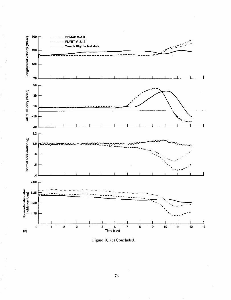
_, 1600

'_ 1300

C

_5 100

01

0.J

0

o>m

E

¢=.J

7O

50--

30--

10

-10 --

-30

1.2 m

i 1.0.8

E .60

Z

.4

7.00 --

-- BEMAP V-1.0

........... FLYRT V-5.13

Trends flight - test data

mm=

I I I 1 I I I I I I I I I

_o e 3.50

N

"-" 1.750

"I-

I I I I I I I I I I

°_

I I

0

(c)

roll

_, ..° .o

,_ *. o

'_ ".*oo.,.°o"

I I I I I I I I I I I I

,., ......... i°,,,..°o,o.,., ........ o°oo,o., .....

o .......... ° ...... ..°°

_ .o

%% °"....,,,..."°'*'

%

I I I I I I I I I I I I1 2 3 4 5 6 7 8 9 10 11 12

Time (sec)

Figure 10. (c) Concluded.

I13

73

6O

n

E40

3O

62.00

o 58.250

0

=_56.50"O

cm53.750,-I

51.00

8O

7O

"0

" 60

50

60

50.>

_e"6 40O

..... BEMAP V-l.0

........... FLYRT V-5.13

Trends flight - test data

....°'°,..,..,,,,,, ,,,., ,,°,,.,,°-, • ",'.°.° .... ....°..° ,..°.,°°.,".., .

• *.*.,. ,.° ,'..°°..° °,., . ,°° .°..,°., .°

I I I I I I I I I I I I I

I I I I I I I I I I I I I

n - ,_,,

t

30 I I I I I I I I I I I I0 1 2 3 4 5 6 7 8 9 10 11 12

(a) Time (sec)

I13

Figure 11. (a) Responses to collective doublet at 60 kts.

74

20

"G

"_ lOq)

-" 00

-10

e-

Q.

1

-1

BEMAP V-l.0

........... FLYRT V-5.13

Trends flight - test data

____.-="" _

..°'%

.....'° "°

I I I I I I I I I I I I I

,o

I [ I I I I I I I I [" I

"G

o ....¢,

G)

-10 --

m>,.

-2O

297.00 --

E 294.25 --

291.50Q.¢0

o 288.75 --

286.00

(b)

..%

7 -- "°''. %

•..-, - ."o _._

o. ,"• .o. o"

I I I I I I I I [ I I I J

I I I I1 2 3 4

I. o.*'S % ." ".

-- .. , -- • :

% • '.

,qs .°.°

I I I I I I I I5 6 7 8 9 10 11 12

Time (sec)

Figure 11. (b) Continued.

I13

75

9L

I

•p0pnlouo D (o)" I I zan_!::l

(0es) etULL_1. 14 01. 6 9 L 9 S

I I I I I I I I£ g I.

I I I I

,°

I I I I I I I I I I I I

.,• _'ll l

__ if:" "..:¢

¢,..

..

..

°.

I I I I I I I I I I I I I

""'"___

'w__"a "q d"_'_q 'J'_'_ "m _ _ _ _ _ _ _ _? _ _ _ _ _ _ _ _ _ _ _ _ u _ _ --

(0)

Z

0

=_

00

0

r"

<

00

0

01.1. t-o,,-,I

(,Q

E0_1.

08_

0

OH.

I I I I I I I I I I I" 1 0

..; o,,,.., OOt .5"• .,_ ¢_

t,,-

elep lsel - lq6!ll spueJJ. OOg....... , ... •

•a _ £1.'S-A J.HA'I=I ...........

O"I.-A dVIN:_BOOg

6O

o 500

0

• 40

3O

5O

A

O

O

"_ 40"D

C0..I

30

7O

_ -- .... BEMAP V-1.0

........... FLYRT V-5.138 •

_- "- .... Trends flight - test data

------------4 ,<-- ............ ----------.,• • _ f o° %,

.... • .....o ,o°,,....,,, ..... ,." - Ss • o,, ,,, ..... *...,., .... ......... o o. ..,

.°

• o"

I I I I I I I I I I I I I

• .° _,,,ooo°0,.

,°0,0 o,o o ,°°°° s =e - _.._ *..o °,°,°°%° °,°°,°,%°°.o° , .oo.0 .° ,,° • ,_ °oo °°,. ,o.°°, ,,., ° 0 o

I I I I I I I I I I I I I

5O

80

.........•"...".7.;...'.'......."..'..'...""" "--.'..,, ,-..'" ........"..;..',.'..'..'....'..'...-..'..-'-.i-"°- *= _ _..e " .°

• o .o.,o°,°.o.

I I I I I I I I I I I I

70

._"6

N 60o

500

(a)

............... • °.°° .... o,,.°°,°,°,o°°.,°°°° .......... ,,o.o ........ °,.° ............................... ooo .... ,°..,,..

I I I I I I I I I I I I1 2 3 4 5 6 7 8 9 10 11 12

Time (sec)

Figure 12. (a) Responses to lateral doublet at 120 kts.

I13

TT

20--

AOa_ 10--

"0

_ 0

_ -10 --

-20

• 3

1

t--O

,,!

-3

10

o

.=

t_>-

-10

293

i

.... BEMAP V-l.0

........... FLYRT V-5.13

- - _ _ Trends flight - test data

• s _ ," .° q._ •

I I I I I I I I I I I i I

/ ... •

Io.

I.° • o •

F_ v. .........,k° °" •°°°" •

I I I I I I I I I I I I I

A

E 292

"0

291Q.¢n

290

289 I0 1

(b)

I I I I I I I I I I I I I

I I I t I I I I I I ]2 3 4 5 6 7 8 9 10 11 12

Time (sec)

I13

Figure 12. (b) Continued.

78

--- 240O4)

•_' 230

220

O.J

210

3O

2o

>

10

.J

1.300

1.1754-*

1.050O(Jm

B

E .9250

Z

.80O

1.00

.... BEMAP V-1.0

........... FLYRT V-5.13

Trends flight - test data

I I I I I I I I I I I I

m

4, °_ • ."

"°%_° • •, g_Q

I I I I I I I I I I I I I

_E_lt Itt

..°°." °°° I4,_ °° . ° °_

-- pl.°°

• _ 1['° _ °o°.,°.°.°, .°.° '

• , . ..... .,;" Iv" .....................

IP

I I I I I I I I I I I I I

= _ -0.25

o° -1.50"Go_OC'O

O'_

•_-.-_ -2.75C

°°,°.° ° • . . ° .

............ ., ..'_'J*"'",¢:..:.. , ...................................._-_ _ *,,''.. ..... .°°'° ,,,,

-4.o0 I I I I I I 1 I I I [ I0 1 2 3 4 5 6 7 8 9 10 11 12

(C) Time (sec)

Figure 12. (c) Concluded.

I13

79

6O

0

o_ 40

m, 30

20

6O

.2 50m0

O

"_ 40._"O

_ 3o0,.J

2O

70--

6O

A

v

-_ 5O"0

4O

30

80m

,._ 7O

:>•= 600

m0

o 5O

BEMAP V-l.0

........... FLYRT V-5.13

Trends flight - test data

• oo,,oo ..*," ','.,o,"*, ,,',°'o "oo'," ',oo o*",-'°OO,oo,O_,o,o,,o °'°,°, o..°. o, o ,o, ,,, oo,I °.oO,o.°. o..o° ,,

1 I I I I I I I I I I I

4 _ ..,,o// \',...:,-- :.....•. ........ ._g \ " "< .:,,'L'_:...................-"_ ":" --:-.......

_._> _'..."

I I I I I I I I I I I I I

400

(a)

I I I I I I I I I I I I 1

I I I I I I I I I I I I I1 2 3 4 5 6 7 8 9 10 11 12 13

Time (sec)

Figure 13. (a) Responses to longitudinal doublet at 120 kts.

8O

2O

-" 0O

-10

10

AO

0

J_

a.

-10

10

0

_ 0

.m

m

-10

400

E300

_O

200

(b)

100

I I I

BEMAP V-l.0

FLYRT V-5.13

Trends flight - test data

• L .......... ';;"

I I ] I I I ] I I

1 I I I I I I I I I I I r

I I I I I I I I I I I I I

I I I1 2 3

I I I I I I I I I4 5 6 7 8 9 10 11 12

Time (sec)

Figure 13. (b) Continued.

I13

81

_" 240.00

.__ 212.500

m

185.0m

._¢'U

157.5C

0,.1

130.0

40.0

4)

27.5

o 15.0o>

u(13

2.5f13--I

-10.0

m

BEMAP V-l.0

........... FLYRT V-5.13

Trends flight - test data

_ __--..._,,,, ;,,, ---_

I I I I I I I I I I I I I

,D

E

00m

m

E

z

•.- ,c_0

(c)

Is=,, =` .b %j,.,. .... ,... %

,.. ...",,,

__ ............ .

I I I I I I I I I I I I

1.600 --

1.325

1.050

.775

.500

1

,,j,D •

I I I I I I I I I I I I

0

-1

-2

-30

..° .... 0,,°°°. .o'° °''°'*°'''_°°''° °'°°"

I I I I I I I I I I I I1 2 3 4 5 6 7 8 9 10 11 12

Time (sec)

I13

Figure 13. (c) Concluded.

82

60--

A

.9 50

O

40_1

A

.2O

O

t_

._.R"O

.==O'}e-O.-i

30

50--

BEMAP V-1.0

................ FLYRT V-5.13

Trends flight - test data

_e

,,,,oO° ,,'o, .... ,oo°'" "O*o° ,,,.,°,,,O,Oo,,Oo,.

o-° .,,. o.,.,,,°,,,,%°'°o.°° ,..° °,, o,°,°,..,o,,.,o ,' °o.,. ,%.o,°,°,,o' *-°°.,**.o°'°

I I I I I I I I I I I I I

4O

3O

o,,*'°'*.".°..° ,.°°

o.. ..,..,.°°.,o...... ,,,o°.'°o. .*** _ I_" _'_,_ *.o° .,o.,

Oo,, • ° °°,°.°°,., .°_ _% °,o°,,.o,.OO •

• _ "" °,,.,°°.oOO,°o.***°,.°" •

I I I I I I I I I I I I I

80--

'tO

D.

7O

6O

5O

4O

_ -..-.... . ..-....._ ....,..

I I I I I I I I I I I I

80--

A

G)>_= 70(3

_¢"6o

(a)

;_-.-'_.-`_.._...._-:..L...;..'_._:-:_._.:_....-`..L_`-..-.:_:_.L_.L_L._L.L_L.L.L_L._L.L_L_L.L._L._L._L-_:6o I I I I I I I I I I I I

0 1 2 3 4 5 6 7 8 9 10 11 12

Time (sec)

Figure 14. (a) Responses to directional doublet at 120 kts.

I13

83

10--

o

.=-- -100O:

-2O

2O

(U

•-_ lo0

.=,- 0.-20...

-10

20

"G" 10

IIU

--- 0

_ -10

-2O

300

E

"O

E 290(/)

0IIC

(b)

280

.... BEMAP V-1.0

........... FLYRT V-5.13

Trends flight - test data

.... _.. t._ ',_'_.q_

•.................'_,j/ ...... _.%." • ,,b %°°.,'°

I I I I I I I I I I I t I

-- __ n

I I I

,°o,,°'°

,,,o,,,,,,''"

-_._ ..- ,,,, __• °.,

I I I I I ] I I I

.°°o

.oo o._. .

%......'

I I I 1 I I i I I I I I I

,o

°%

"%

I I I i I I I I I I I2 3 4 5 6 7 8 9 10 11 12

Time (sec)

Figure 14. (b) Continued.

I13

84

•_" 280.0 --

262.5

"_ 245.0I¢U

._c1D

._=227.5C0

.J210

BEMAP V-l.0

........... FLYRT V-5.13

-- _ Trends flight - test data .....""

=,

-- =.

b,, l,.t Id I_ _' "'...

I I I I I I I I I I I I I

40--

¢)G)

20

0

z>o

.=

• s "_."r% p

A

v

t-O

.m

m

00o=mm

.EOZ

3 --

m

iiii

I I I I I I I I I I I I

0 m

o=-2.50

t,-, D

_'_"= .-_ -3.75O

"r

°.°

.°

-'":-'::....._ ..... . .......... _ .

%

I I I I I I I I I I I I0 1 2 3 4 5 6 7 8 9 10 11 12

Time (eec)

Figure 14. (c) Concluded.

I13

85

60

so

40

50

U

U

U

"_ 4OF-"O

C0

-J

30

7O

m

BEMAP V-1.0

........... FLYRT V-5.13

Trends flight - test data

o o*,,,"°°°*.o°*,,., ,, ,,o.oH o,o°O" " oo, ,°.°oo o°,. o °oo°°O o, oo .Oo O.oo,..,°°,°

°o°,,o • , ,,°,,,,°°°o,,O., °°o"o. °°o

I I I I I I "'i"'"....... I°" I I I I

.,.'.

• °*_ • _t'°

.... ,." # • •°, "'°""., ° °,°.,.o°,°,,,., ,o,. ,., .,.'* "-, . *.. °" I ".

°°°°°°°°°°. o° ,o°.,o°.°. o o°°o°, °°o . ._ • °°°°°°° •_. • °

°°°° • • I_ _

I I I I I I I I I I I I I

"O4)

a.

50

90

•"_0 °" "_'° "%',• • o I "a'#' .,,_ -- *b •• oo:.-,r....', 7.S,, 7.S•. ".7..'..'.7.--.... 7..',:..'..'..'..:,:

",...

oo,,-°

I I I I I I I I I 1 I I I

8O

4)>

= 70O

"6o 60

500

(a)

i

t|

1 I I I I I I J I 1 I I1 2 3 4 5 6 7 8 9 10 11 12

Time (sec)

Figure 15. (a) Responses to collective doublet at 120 kts.

I13

86

0

On"

-lO

10--BEMAP V-1.0

........... FLYRT V-5.13 ....j,,_,.Trends flight - test data ."" ". ,'" ,," _"

"°%°°°°.°°° _ °o

_ _.,.., ,..,,. __ ,,. ,,...,... -.. ................. i.,, -_...=_"- t_.. .-

. °" _

ID

• -1

e-

o_o.

lO

AO

_ o

-lO

4 B

I I I I I I I I I I I I I

Io. ""°)'°o • • .°"/,,\.... _ .." -- °

_..,,.._.

I I I I I I I I I I I I I

F._'_.,.. ..."....

:1 , ° ,: °¢°a.'

... _.. ,,,,.. -\/..... "" -.. ..... ,_.-_.....-. .. ';' _ F

I I I I I I I I I I I I

298.00 --

A

E 295.25

292.50

289.75

287.00

(b)

l" - ,%

-- %% t t

I I I I I I I I I I I I0 1 2 3 4 5 6 7 8 9 10 11 12

Time (sec)

Figure 15. (b) Continued.

I13

87

A 230

•"_ 2200

>

r-

_5 210

O_CO

,.I

200

40.0

27.5

.__° 15.0

_oIU>

_ 2.5o

.-I

-10.0

1.4

t-o= 1.1

00

0Z

.5

4,,e_ 1

= o= -1

•= ._ -30"r"

-50

(c)

BEMAP V-1.0

............ FLYRT V-5.13

Trends flight - test data

I I I I I I I I I I I I I

m ."'"'°'°

°_ _;**%

-- o°,,o,.,o _. .1..4r

I I I I I I I I I I I I I

It*v _I" ' ".

_ _, ...... :,,,, ".t

_l I,"" °°° "._

-- o" *, °

I I I I I I I [ I I I I

I ] I I I I I I I I I I1 2 3 4 5 6 7 8 9 10 11 12

Time (see)

I13

Figure 15. (c) Concluded.

88

A

.2mO

o

60--

5O

40

3O

20--

10

e#

0

o -10n-

-2O

0 3

"0"" 1

.=J_

o -1O.

-3

BEMAP, input at swashplate

.. •.......... BEMAP, input at stick

:t "_ _ Trends flight - test data"ij'_-,.,.. .... ,...,• "t •

I I I I I I I I I I I I I

"0_ 2

n nm -_

I I

_,_ . ........ ."..'._ ..__

I I I I I I I I I I

f .

• %

• %

| I I I I I I _ I I I I I

0

• %

• • •'_% _ S SS

._ ,,,% t/. s

I__........ _/." / \

I I I I I I I I I I I I I1 2 3 4 5 6 7 8 9 10 11 12

Time (sec)

Figure 16. Lateral doublet at 60 kts, input at stick.

I13

89

20I°0

-20==r-m -40t13

:S -60

Flight results

.... BEMAP V-1.0

.......... FLYRT V-5.13

PB/LAT /.

i l l ,I l i i i I

,,__mm_2oo_1oolOOot" PB/LA_

I I i II I i I II

or-==4)

J::O

O

1.0

.8

.6

.4

.210-1 100 101

Frequency (rad/sec)

80 I VB/LAT .."._0

_ -40i J I il l l I il

-s°ivB A-150 .... / -_e -250

-350-450

-550 i i J i I I i i"f'l

J=0

0 .4

.2 I _ i , , I i i i_/i I10-1 100 101

(a) Frequency (rad/sec)

Figure 17. (a) Comparison of BEMAP responses with flight at hover.

9O

Flight results

0Am

-2o

•, -40e.-o_ -60t_

-60

BEMAP V-1.0

FLYRT V-5.13

5O

-50

c/)

m -150J_a.

-250

I QB/LON '-

1.0

o • .8t-

.6J¢OO .4

.210-1

QB/I.ON _

100 101

Frequency (racl/sec)

6OAm

20"O

c -20

-60

150

_ 5O

_ -5om -150m

g. -25o-350

I i i _ i I t' , i i I

E UB/LON

I , , i il i , i tl

0

e-0

<.)

(b)

1.0

.8

.6

.4

.210-1

I UB/L I

100 101

Frequency (rad/sec)

Figure 17. (b) Continued.

91

20

0

-2O

40

40

150

5O

-50

-150

Flight results

.... BEMAP V-l.0

.......... FLYRT V-5.13

C

m

1.0

o .8

| .60

.4

.2 / i n f fl i _ _ _I10"1 100 101

Frequency (rad/sec)

6ofwcol=_ 40

20"_ 0

_= -20 I I I I

_-200

===_ --3o0

400 _ I

¢ .8 -0C

| .60

.4

.2 i n n ii n i a nl n n i nl10-2 10-1 100 101

(C) Frequency (rad/sec)

Figure 17. (c) Continued.

92

-- Flight results

.... BEMAP V-1.0

.......... FLYRT V-5.13

0

m-20

-4O

Cm -60W

-8O

pB o.......?..

.... _:::;_.:...""_. .... _ .............

/ I i , ,I t , I , I

45O

O) 250

50mp,

-150I PB/LON _-

t , , iI , , , II

1,0

o .8¢.=

.6c-o

0 .4

.210-1 100 101

Frequency (rad/sec)

0

m-20

OqD

_ -40_ -60m

lIE--8O

I QB/LAT .- ..

............ .-'" ". ,.,

I I I li J I I II

250

_ 5O

_ -1soO.

-35O

I QB/LA

............... • ...

i , J II , i , ,-I

m .8¢.}c

| .e¢.=00 .4

.210-1 100 101

(d) Frequency (rad/sec)

Figure 17. (d) Concluded.

93

20Im

o

i -20

-40-60

100

m 0(p

-100

-200

-300

oocot-O0

Flight results

.... BEMAP V-1.0

......... FLYRT V-5.13

PB/LAT

,.,..

I I I I I

1.0

.6

.4

.2 I ' _'l I I r ll I10-1 100 101

Frequency (rad/sec)

i i iI

0Am

-2o¢D

_= -40p.m -60:E

-60

5O

o_-50

o

-15o,'1

-250

1.0

Q_: .8

e) .6t-O(.) .4

(a)

Flight results

.... BEMAP Vol.0

......... FLYRT V-5.13

I I ill i i ill _ t I II

,,,,.2 I I I 111 I I I I[ I W _1

10-1 100 101 102

Frequency (rad/sec)

Figure 18. (a) Comparison of BEMAP responses with flight at 60 kts.

94

2OAm

0

_o -20=:Cm -40ca

:S-6O

150

50

-50Wr.

a.-150

4)o .8r-

a) .6t-o

W

G)

_= o.u¢-m -20m

:E-4O

150

350

-55oJ¢a.

-750

Flight results

.... BEMAP V-l.0

' •......... FLYRT V-5.13

I RB/PED

.,..../,, •

I I i_l a , ,,I ,

I RB/PED

%%

"OIRB'P D.4

.2 i i

10-1 100 101

Frequency (rad/sec)

1.0

G)O .8C

| .B.C:O

(J

(b)

40 IWB/CO_

20 -

WB/COL

% *..... .*

WB/COL _

.2 I I Jl t10 "1 100 101

Frequency (rad/sec)

Figure 18. (b) Continued.

I i il

, ill

i i,l

102

i t l[

95

Flight results

.... BEMAP V-1.0

.......... FLYRT V-5.13

-o -20

C

_ -40

-60 I _ _1 _ _ _1 I Ill

50 I PB/LO_

-150

-350-s.0

a. -750 i i wi I i i i i I i I ill

OC

.¢:O

o

1.0

I PB/LON

.6

.4

.2 !

10-1

Ill I t Ill

100 101

Frequency (rad/sec)

I I I II

10 2

.010 "-20"0

-40,mC

o_ -60

:E -80 I I I w l i i i i I

"_ -150

-350

-550_. -750

-950 I , i ,I , , , I I

I I I II

I I I I I

¢.)t-

t-O

(c)

1.0

.8

.6

.4

.210-1 100 101

Frequency (rad/sec)

Figure 18. (c) Concluded.

96

Flight results

.... BEMAP V-1.0

.......... FLYRT V-5.13

m'-" 20 t RB/PE_

-o -20

Cm --40

=E -60 i J ,ll I I Ill I I IJl

-5OA

-_ -250

U_

.450Q.

-650

I RB/PE_

00C

J=0

o 1.0.4.6.8I RB/PED_jj_/_I

.2 ' , jl , , i,l ,10"1 100 102

Frequency (rad/sec)

.--. 40 f WB/CO_

tin :_ ....... _ _:_.

20-0"0

C

_ -2o

_ -40 i I K ii i J i el I

250

o_ 50¢D"10

-150¢Du)

-350Q.

-550I WB/CO

I i J Jl i , ,,I i

ow_,..1.0.8.6t wB/CO-0.4

.2 I10"1 100 10 2

(b) Frequency (rad/sec)

Figure 19. (b) Concluded.

i 1,1

101

i III

t i il

I I II

101

98

2Om

o

•o -20:1

o) -40

:E-6O

Flight results

.... BEMAP V-1.0

.......... FLYRT V-5.13

I PB/LA_

.....

f i Ill I till i I ,tl

5OA0'}

-50

-15o

o. -250I PB/LA_

.."1 ..........I I ,I : I I I II I I Itl

{JI¢

a)t-O

1.0

.8

.6

.4

.210-1

i t I ill I i iii J

100 101

Frequency (rad/sec)

I i_l

102

,..,. 40 I QB/LO_

m20-

"O

.._: of..

o_ -20:E

-40 I i t il I I I II i I Itl

A 50 I QB/LO_..,

-5o -

-150 _--,... ,,,,7,,a. -250

I I ili I I ill i t ttl

(,,)f,.

ot-O

(,,)

(a)

1.0

.8

.6

.4

.210-1 100 101

Frequency (rad/sec)

Figure 19. (a) Comparison of BEMAP responses with flight at 120 kts.

97

Form ApprovedREPORT DOCUMENTATION PAGE OMBNo 07o4-0188Public reporting burden for this collectionof information is estimated to average 1 hour per response, including the time for reviewing instructions, searching existing data sources,gatheringand maintaining the data needed, and completingand reviewing the collectionof information. Send comments regardingthis burden estimate or any other aspect of thiscollection of information, including suggestionsfor reducingthis burden, to Washington Headquarters Services, Directoratefor information Operations and Reports, 1215 JeffersonDavis Highway, Suite 1204, Arlington, VA 22202-4302, and to the Office of Management and Budget, Paperwork Reduction Project (0704-0188), Washington, DC 20503.

1. AGENCY USE ONLY (Leave blank) 2. REPORT DATE 3. REPORT TYPE AND DATES COVERED

April 1995 Technical Memorandum4. TITLE AND SUBTITLE

Development and Validation of a Blade-Element Mathematical

Model for the AH-64A Apache Helicopter

6. AUTHOR(S)

M. Hossein Mansur

7. PERFORMING ORGANIZATION NAME(S) AND ADDRESS(ES)

Aeroflightdynamics Directorate, U.S. Army Aviation and Troop

Command, Ames Research Center, Moffett Field, California

9, SPONSORING/MONITORING AGENCY NAME(S) AND ADDRESS(ES)

National Aeronautics and Space Administration

Washington, DC 20546-0001 and U.S. Army Aviation and Troop

Command, St. Louis, MO 63120-1798

5. FUNDING NUMBERS

505-59-36

8. PERFORMING ORGANIZATIONREPORT NUMBER

A-95034

10. SPONSORING/MONITORINGAGENCY REPORT NUMBER

NASA TM- 108863

USAATCOM TR-94-A-022

11. SUPPLEMENTARY NOTES

Point of Contact: M. Hossein Mansur, Ames Research Center, MS 211-2,

Moffett Field, CA 94035-1000; (415) 604-6037

12a. DISTRIBUTION/AVAILABILITY STATEMENT

Unclassified-Unlimited

Subject Category - 01

12b. DISTRIBUTION CODE

13. ABSTRACT (Maximum 200 words)

A high-fidelity blade-element mathematical model for the AH-64A Apache Advanced Attack

Helicopter has been developed by the Aeroflightdynamics Directorate of the U.S. Army's Aviation and

Troop Command (ATCOM) at Ames Research Center. The model is based on the McDonnell Douglas

Helicopter Systems' (MDHS) Fly Real Time (FLYRT) model of the AH-64A (acquired under con-

tract) which was modified in-house and augmented with a blade-element-type main-rotor module. This

report describes, in detail, the development of the rotor module, and presents some results of an exten-sive validation effort.

14. SUBJECTTERMS

Blade-element; Helicopter, Mathematical model

17. SECURITY CLASSIFICATION

OF REPORT

Unclassified

NSN 7540-01-280-5500

18. SECURITY CLASSIFICATIONOF THIS PAGE

Unclassified

19. SECURITY CLASSIFICATIONOF ABSTRACT

15. NUMBER OF PAGES

9816. PRICE CODE

A0520. LIMITATION OF ABSTRACT

Standard Form 298 (Rev. 2-89)Prescribed by ANSI Std. Z39-18