HAL Id: hal-03182341https://hal.uca.fr/hal-03182341

Submitted on 28 Oct 2021

HAL is a multi-disciplinary open accessarchive for the deposit and dissemination of sci-entific research documents, whether they are pub-lished or not. The documents may come fromteaching and research institutions in France orabroad, or from public or private research centers.

L’archive ouverte pluridisciplinaire HAL, estdestinée au dépôt et à la diffusion de documentsscientifiques de niveau recherche, publiés ou non,émanant des établissements d’enseignement et derecherche français ou étrangers, des laboratoirespublics ou privés.

Developing states and the green challenge. A dynamicapproach

Alexandra-Anca Purcel

To cite this version:Alexandra-Anca Purcel. Developing states and the green challenge. A dynamic approach. RomanianJournal of Economic Forecasting, 2020, XXIII (2), pp.173-193. �hal-03182341�

1

Developing states and the green challenge. A dynamic approach

Babeș-Bolyai University, Faculty of Economics and Business Administration, Teodor Mihali

St. 58-60 400591, Cluj-Napoca, Romania

Université Clermont Auvergne, CNRS, IRD, CERDI, F-63000 Clermont-Ferrand, France

*Corresponding author: alexandra.anca.p@gmail.com

Abstract: This paper studies the effects of output, urbanization, energy intensity, and

renewable energy on aggregated and sector-specific CO2 emissions for a rich sample of

developing states. We employ the recently developed GMM panel VAR technique, which

allows us to tackle the potential endogeneity issue and capture both the current and future

impact of indicators on CO2 via the impulse-response analysis. On the one hand, robust to

several alternative specifications, the findings indicate that output, urbanization, and energy

intensity increase the aggregated CO2 emissions, while renewable energy exhibits an

opposite effect. Moreover, regarding the CO2 responsiveness to output and urbanization

shocks, the pattern may suggest that these countries are likely to attain the threshold that

would trigger a decline in CO2 emissions. We also reveal heterogeneities related to both

countries’ economic development and Kyoto Protocol ratification/ascension status. On the

other hand, the sectoral analysis unveils that the transportation, buildings, and non-

combustion sector tend to contribute more to increasing the future CO2 levels. Overall, our

study may provide useful insights concerning environmental sustainability prospects in

developing states.

Keyword: CO2 emissions; urbanization; energy efficiency; renewable energy; developing

countries; environmental Kuzents curve; GMM panel VAR.

JEL Classification: Q01, Q53, Q56, O13

Acknowledgments: I am indebted to the Editor (Corina Saman), two anonymous referees,

participants at ”The Thirteen International Conference on Economic Cybernetic Analysis:

Sustainable Growth in The Current Socio-Political Context (SGSP2018)” held at The

Bucharest University of Economic Studies, and Dorina Lazăr and Alexandru Minea for

valuable comments and fruitful discussions. All remaining errors are mine. Usual disclaimers

apply.

2

I. Introduction

As a global and stock pollutant with the highest share in greenhouse gasses, carbon dioxide

(CO2) emissions are considered the main driving force of environmental degradation.

According to Olivier et al. (2017) report, developing countries such as Indonesia and India

have recorded the highest absolute increase in CO2 emissions in 2016 (6.4% and 4.7%

respectively), followed closely by Malaysia, Philipines, and Ukraine.

Indeed, having the fastest-growing economies, most developing countries experience

complex structural changes that reflect in the mix of various socio-economic processes such

as industrialization and urbanization. For example, according to the United Nations World

Urbanization Prospects (2014)1, the urban population in 2014 accounted for 54% of the total

world population, and it is expected to rise at about 66% by 2050. Additionally, considering

the worldwide ongoing urbanization process, Asia and Africa seem to exhibit the fastest rate

of urbanization. Overall, these changes strongly connected with the industrialization process

also imply an intensification and a shift of economic activities towards urban conglomerates,

demanding the use of more energy resources, which in turn may reflect in higher pollution.

Consequently, some of the key factors that can help mitigate pollution include the gradual

replacement of classic fossil fuels with more carbon-neutral alternatives, the increase of

renewable sources in the energy mix, and the improvements in energy efficiency. In this

regard, the renewable energy and energy efficiency projects implemented between 2005 and

2016 in developing economies, and supported at the international level, are expected to

reduce greenhouse gas (GHG) emissions by 0.6 gigatons of CO2 per year by 2020 (United

Nations Environment Programme, 2017)2. Likewise, based on the same report, approximately

75 developing or emerging economies have implemented policies or programs that

incorporate renewable energy and energy efficiency technologies.

Looking at developing countries' positions vis-à-vis the global environmental

challenges and the main related tools designed to address them, they differ in certain features

from developed countries. On the one hand, developing states being Non-Annex I parties of

the Kyoto Protocol do not have binding commitments to reduce or limit their emissions,

compared to their industrialized counterparts. Nonetheless, they may voluntarily comply, and

the advanced economies that choose to support them in fighting global warming may also

benefit in terms of the fulfillment of their commitments. For example, the Kyoto Protocol's

1 https://population.un.org/wup/publications/files/wup2014-highlights.pdf 2https://wedocs.unep.org/bitstream/handle/20.500.11822/22149/1_Gigaton_Third%20Report_EN.pdf?sequence

=1&isAllowed=y

3

well-known Clean Development Mechanism (CDM) is designed to jointly involve

developing and developed economies in fighting climate change through the implementation

of various green projects.3 On the other hand, following the Paris Agreement's adoption under

the umbrella of the United Nations Framework Convention on Climate Change (UNFCCC),

both developing and developed economies are required to put the efforts and fight together

against the imminent threats of climate change. As such, the Paris Agreement may represent

one of the most powerful instruments adopted so far concerning developing countries and

their active role in combating and mitigating the harmful effects of global warming.

Taking stock of the above mentioned, the goal of this paper is to assess the

responsiveness of CO2 emissions following external disturbances to output and urbanization,

assuming a transmission channel that incorporates two of the key elements used in mitigating

environmental degradation, namely the renewable energy and energy efficiency. In doing so,

we employ the recently-developed Generalized Method of Moments (GMM) panel Vector

Auto-Regression (VAR) approach of Abrigo & Love (2016), which allows us to explore the

essential dynamics and tackle the potential endogeneity between indicators. The technique is

applied for a comprehensive group of developing countries, within a modified Stochastic

Impacts by Regression on Population, Affluence, and Technology (STIRPAT) framework,

which along with the Environmental Kuznets Curve (EKC) hypothesis4 helps us to provide

the necessary economic foundation for the assumed innovations’ transmission mechanism

required to identify the key structural shocks. Furthermore, opposite to a sizeable empirical

strand of literature that independently examines the nexus between CO2 and growth

(urbanization) via the classical (urbanization-related) EKC hypothesis, we jointly test these

two well-known hypotheses. Indeed, building on the general belief that a vast majority of

developing economies have not yet reached the maximum level of growth (urbanization) that

would ensure a decrease in pollution, this approach via the computation of impulse response

functions (IRFs) allows us to assess whether this will be feasible or not in the future. As well,

motivated by the ongoing structural changes that developing countries experience, we focus

on aggregated and sector-specific CO2, as they may provide us with complementary insights.

3 As a result of the CDM green projects (i.e., projects aimed at reducing emissions) implemented in developing

countries, the Annex I parties can buy Certified Emission Reduction (CER) units, which in turn help them to

meet some of their commitments of emission reduction (Carbon Trust, 2009). 4 The classical EKC hypothesis states that the relationship between environmental degradation and economic

growth follows a bell-shaped pattern (Grossman & Krueger, 1991).

4

Our findings can be summarized as follows. First, although output and urbanization

shocks trigger a rise in the current and future levels of CO2, the effect may reverse, and in the

long-run, a bell-shaped pattern seems to be at work in terms of the CO2 responsiveness.

Moreover, the green actions that developing countries have taken in the last decades, in

particular those related to renewable energy sources, seems to reduce the cumulated CO2

emissions both on the short- and long-term horizon. However, considering that the positive

disturbances to energy intensity are associated with an increase in CO2, more attention

should be paid to energy efficiency, by attracting and implementing more related projects.

Also, while the results confirm the persistence in CO2, a permanent shock to its dynamics

causes only a small increase in the future emissions levels.

Second, we examine the robustness of these findings by changing the order of

variables into the transmission channel, altering the sample in several ways concerning both

N and T dimensions, and controlling for an extensive set of exogenous factors. According to

IRFs, the shocks to output, urbanization, energy intensity, and CO2 have the same cumulated

increasing effect on CO2, opposite to positive disturbances to renewables that trigger a

cumulated decrease in CO2. Likewise, the CO2 response to GDP and urbanization shocks

tends to exhibit a bell-shaped pattern in the long-run, indicating that the related EKC

hypothesis may be validated.

Third, we find that the results are sensitive to both countries’ level of development

and the Kyoto Protocol ratification/ascension status. On the one hand, overall, the IRFs show

that low income economies might experience a more moderate increase in pollution in the

long-run than lower-middle income states. Besides, in low income states, the results seem to

be compatible with the EKC hypothesis, especially for urbanization. On the other hand, the

countries that ratified or acceded to the Kyoto Protocol before it entered into force may also

be those which have been more actively engaged in combating pollution, given that both

output and urbanization are more likely to display a threshold effect on CO2 (i.e. validate the

EKC hypothesis in the long-run). Indeed, this may also suggest that these states faced the

effects of increasing pollution earlier and, thus, decided to become more actively involved in

combating climate change sooner than their counterparts.

Finally, despite the positive response of aggregate CO2 to output and urbanization

shocks, when the sectoral components of CO2 are taken into account, the findings appear to

be much more diverse. In particular, we find opposite results for the other industrial

combustion and power industry sector, namely external disturbance to both GDP and

urbanization lead to a cumulated decrease in associated CO2. Thus, overall, the disaggregated

5

CO2 analysis indicate that transportation followed by construction and non-combustion

sector are more prone to contribute to increasing CO2 pollution in developing economies.

The remainder of the paper is organized as follows. Section 2 reviews the related empirical

literature. Section 3 provides the STIRPAT framework, discusses the research methodology,

and describes the data used in the analysis. Section 4 presents the baseline empirical findings.

Section 5 examines the robustness of these findings. Section 6 explores their sensitivity.

Section 7 analyzes the sector-specific CO2 dynamics following exogenous shocks to other

system variables, and the last section presents the concluding remarks.

II. Literature review

In the light of the vast body of empirical literature on the environmental degradation

determinants, this section aims to review some of the most recent empirical studies that tackle

the impact of output, urbanization, (non-) renewable energy, among other explanatory

factors, on environmental degradation. More precisely, we mainly focus on works that

explore this nexus for developing5 economies in the context of STIRPAT and/or EKC

hypothesis (both the classical and urbanization related ones). As well, given that the output

appears in almost all studies as one of the main determinants of environmental degradation,

we split the literature into two main parts, namely the (i) output-urbanization-environmental

degradation nexus, and (ii) output-(non-)renewables-environmental degradation nexus.6

First, regarding the impact of economic growth and urbanization on environmental

pollution, we further split the studies into two sub-categories. Thus, the first strand of

literature tackles the papers that extend the baseline STIRPAT equation and/or EKC

hypothesis to capture the effects of the urbanization process. In this fashion, researchers such

as Lin et al. (2009), Li et al. (2011), Wang et al. (2013), Wang & Lin (2017), among others,

using time-series data on China reveal that, overall, both urbanization and economic growth

exacerbate the environmental degradation. The authors employ techniques such as ridge

regression, partial least-squares regression, or VAR model. Likewise, the findings of Talbi

(2017) for Tunisia and Pata (2018) for Turkey show that urbanization increases CO2

pollution, while economic growth exhibits a nonlinear effect on CO2, validating the EKC

hypothesis.

5 The term “developing” is used with double connotation, meaning that it refers to both developing and

emerging countries. 6 We note that the studies that comprise, along with the output, both urbanization and (non-) renewable energy

as explanatory factors of environmental degradation, are included in the category that we consider most suitable.

6

Furthermore, making use of STIRPAT framework, several works (see e.g.

Poumanyvong & Kaneko, 2010; Liddle, 2013; Iwata & Okada, 2014; Sadorsky, 2014a; Wang

et al., 2015; among others) examine the effects of growth and urbanization on environmental

degradation, using either samples of developing countries or mixed samples comprising both

developing and developed economies. However, in most cases, the findings unveil that both

variables have a positive effect on environmental degradation. Also, it is worth noted that

concerning economic growth, Liddle (2013) and Wang et al. (2016) find evidence in favor of

the EKC hypothesis. Also, scholars such as Li et al. (2016), Awad & Warsame (2017), Joshi

& Beck (2018), among others, study the relationship between pollution and growth in the

context of the EKC hypothesis, while controlling for the effects of the urbanization process.

The authors apply either parametric or semi-parametric panel data techniques, and, most

frequently, environmental degradation is proxied by CO2 emissions. Overall, the findings

seem to be mixed with respect to the EKC hypothesis's validity, whereas urbanization tends

to increase the pollution levels.

The second strand of literature focuses on testing the urbanization-related EKC

hypothesis, whether or not this is done within the STIRPAT context. In this manner, the

findings provided by Martínez-Zarzoso & Maruotti (2011) support the urbanization-pollution

EKC for 88 developing states spanning over the period 1975-2003. Opposite, Zhu et al.

(2012) and, more recently, Wang et al. (2016) find little evidence in favor of urbanization-

CO2 and urbanization-SO2 EKC hypothesis, respectively. Besides, employing the panel

VAR analysis, Lin & Zhu (2017) study the dynamic relationship between industrial structure,

urbanization, energy intensity, and carbon intensity for 30 provinces of China spanning over

the period 2000-2015. Concerning the carbon intensity response following external shocks to

the other variables, the IRFs reveal that both urbanization and industrial structure decrease

the carbon intensity, while energy intensity disturbances increase (decrease) on impact (after

three years) the carbon intensity. According to twenty years horizon FEVDs’ results, only

urbanization exhibits a bell-shaped pattern on carbon intensity. Also, the findings provided by

Chen et al. (2019) and Xie & Liu (2019) show that urbanization exhibits nonlinear effects on

CO2 for 188 Chinese prefecture-level cities and 30 Chinese provinces, respectively.

Second, the present study is also related to the body of literature that investigates the

effects of economic growth, non-renewable energy (especially energy intensity), and/or

renewable energy on environmental degradation. In this regard, Shahbaz et al. (2015)

investigate for 13 Sub Saharan African states the link between energy intensity and CO2,

while additionally test the EKC hypothesis. On the one hand, the long-run panel findings

7

unveil that the energy intensity has a positive impact on CO2, while a bell-shaped pattern

characterizes the CO2-GDP nexus. On the other hand, the country-specific long-run results

reveal that energy intensity significantly increases CO2 in countries such as Botswana,

Congo Republic, Gabon, Ghana, South Africa, Togo, and Zambia. Besides, an inverted U-

shaped (U-shaped) relationship between CO2 and GDP is found in South Africa, the Congo

Republic, Ethiopia, and Togo (Senegal, Nigeria, and Cameroon). Antonakakis et al. (2017)

employ the panel VAR approach to investigate the dynamic interrelationship between output,

energy consumption (and its subcomponents, namely electricity, oil, renewable, gas, and

coal) CO2. In doing so, the authors concentrate on a large panel of 106 states spanning over

the period 1971-2011. Overall, for low income group, the findings (based on cumulative

generalized IRFs) reveal that CO2 respond significantly and positively only to output and oil

consumption shocks. On the contrary, for lower-middle income countries, the CO2 seems to

react significantly and positively to output, aggregated energy consumption, electricity

consumption, and oil consumption. Likewise, Naminse & Zhuang (2018) examine for China

the link between economic growth, energy intensity (in terms of coal, oil, gas, and

electricity), and CO2, over the period 1952-2012. The results based on the IRFs analysis

show that coal, electricity, and oil consumption have a positive impact on the future levels of

CO2. In contrast, gas consumption seems to decrease future levels of CO2. The regression

analysis also indicates an inverted U-shaped relationship between growth and CO2, in line

with EKC. Also, Charfeddine & Kahia (2020) investigate the impact of renewable energy and

financial development on both CO2 emissions and growth for 24 Middle East and North

Africa (MENA) states. The computed IRFs unveil a cumulative negative effect of renewables

on CO2, suggesting that renewable energy sources may reduce CO2 pollution.

Moreover, some authors assess the impact of (non-) renewable energy consumption

and output on CO2 pollution using the EKC framework for European Union (EU) states. As

such, the results of Bölük & Mert (2014) for a sample of 16 EU countries indicate that the

consumption of renewables has a positive impact on CO2 emissions, while the EKC

hypothesis is not validated. Conversely, based on a sample of 27 developing and developed

EU states, the findings of López-Menéndez et al. (2014) show, on the one hand, that

renewables have a negative effect on greenhouse gas emissions. On the other hand, the results

suggest that the EKC hypothesis may be at work for those economies which exhibit high

intensity with respect to renewable energy sources. Likewise, for a sample of EU economies,

Dogan & Seker (2016) show that renewable (non-renewable) energy decreases (increases) the

8

CO2 emission, and the EKC hypothesis is supported. As an empirical methodology, the

authors employ panel data techniques robust in the presence of cross-sectional dependence.7

Bearing in mind the present study’s objective, we previously review some studies that

directly or indirectly tackle the effects of output, urbanization, and (non-) renewable energy,

among others, on environmental degradation. However, given that we aim at addressing the

potential endogenous behavior between variables and, thus, consistent with the recursive

order that we impose among them (see subsection 4.2 for details), the study could also be

linked with the strand of research that examines the relationship between (i) output and

urbanization (see e.g. Brückner, 2012; Bakirtas & Akpolat, 2018; among others), (ii) output

and (non-) renewable energy (see e.g. Sadorsky, 2009; Salim & Rafiq, 2012; Liu, 2013;

Apergis & Payne, 2015; Doğan & Değer, 2018), (ii) urbanization and (non-) renewable

energy (see e.g. Shahbaz & Lean, 2012; Sadorsky, 2014b; Wang, 2014; Kurniawan &

Managi, 2018; among others), and as well the papers that focus on efficiency of (non-)

renewable energy (see e.g. Aldea et al., 2012; Jebali et al., 2017; Gökgöz et al., 2018; among

others).

III. STIRPAT framework, research strategy, and data

3.1. STIRPAT framework

STIRPAT is an analytical framework introduced in the literature by Dietz & Rosa (1994,

1997) as the stochastic counterpart of IPAT identity proposed by Ehrlich & Holdren (1971).

According to the I=PAT accounting equation, the environmental impacts denoted by (I) are

determined in a multiplicative way by demographic-economic forces such as population (P),

affluence (A), and technology (T). Nonetheless, over the years, to meet the needs of different

research questions the baseline IPAT/STIRPAT model has encountered many alternative

specifications (see e.g. Kaya, 1990; Schulze, 2002; Waggoner & Ausubel, 2002; Xu et al.,

2005; Martínez-Zarzoso et al., 2007; Lin et al., 2009; Shafiei & Salim, 2013; among others).

First, the classical IPAT equation written for panel data with observed countries over

the period takes the following for

7These findings are also partially supported by the more recent study of Inglesi-Lotz & Dogan (2018) for a

sample that comprises the top 10 electricity generators states from Sub-Saharan Africa. Specifically, the results

show that renewable (non-renewable) decreases (increases) the CO2, but the validity of the EKC hypothesis

over the period 1980-2011 is not supported.

9

Second, the stochastic counterpart of the above accounting identity is obtained by

applying natural logarithm on equation (1). Also, along with this transformation, we

approximate the environmental impacts with a well-known global pollutant, namely the

CO2 emissions. Likewise, we proxy with the share of the urban population in total

population (URB), with the gross domestic product (GDP), while it is captured through

both energy intensity (EINT) and the share of renewable energy in total energy consumption

(RENG). Subsequently, our modify STIRPAT model can be specified as follows

In the above equation, all the variables are expressed in natural logarithm form, while and

captures the potential country-specific fixed effects and the error term, respectively.

Moreover, given that the affluence term is usually expressed via GDP, its square (cubic) term

into the equation allows for testing the well-known EKC hypothesis in its traditional

(extended form). Indeed, the same holds for any explanatory factor, namely adding higher-

order polynomial terms, allows for testing a potential nonlinear effect of the respective

variable on environmental degradation (e.g. the urbanization-EKC hypothesis).

3.2. Methodology

To explore the CO2 responsiveness to other system variables shocks, we draw upon the novel

panel VAR methodology. In this regard, we follow the work of Love & Zicchino (2006) and

Abrigo & Love (2016) and estimate a homogeneous panel VAR model using the GMM

approach. Indeed, this technique gives us the possibility to treat all the variables

endogenously and also to account for the unobserved individual heterogeneity.

The reduced-form specification of a homogeneous panel VAR with individual fixed effects

can be written as follows

Where represents the vector of our four stationary endogenous variables, namely the GDP,

URB, EINT, RENG, and CO2, and stands for associated matrix polynomial in the lag

operator (i.e. the autoregressive structure). is the vector of constants, while and

denotes the vector of unobservables country-specific characteristics and idiosyncratic errors,

respectively. The unobservables may capture the cultural, institutional, and historical

individual country characteristics that are time-invariant. Likewise, we assume that the vector

of idiosyncratic errors possesses the following features: , and

, . Put differently, the innovations have zero first moment values, constant

10

variances, and do not exhibit individual serial and cross-sectional correlation (see Abrigo &

Love, 2016).

Furthermore, in line with Holtz-Eakin et al. (1988), the panel VAR model described

above assumes that the parameters are common across all panel members (Abrigo & Love,

2016). Indeed, this seems to be quite a strong restriction that may not hold when working

with a large number of countries, which are prone to exhibits certain particularities. Thus, the

country-specific fixed effects are introduced into the model to overcome the parameters'

homogeneity assumption. In this regard, the model may be estimated via the fixed effects or

ordinary least squares approach, but the coefficients are likely to suffer from Nickell's bias

(Nickell, 1981)—when estimating dynamic panels, the fixed-effects are correlated with the

regressors, given the lags of endogenous variables (Abrigo & Love, 2016). To alleviate this

issue, we use the Helmert procedure described in Arrelano & Bover (1995), and remove the

mean of all future available country-time observations, by applying forward mean-

differencing (orthogonal deviations). Also, in this manner, we refrain from eliminating the

orthogonality between transformed variables and lagged regressors. Consequently, the

coefficients are consistently estimated by GMM, using instruments the lags of independent

variables (Abrigo & Love, 2016).

3.3. Data

The study concentrates on 68 countries classified by World Bank (2017) as economies with

low and lower-middle income. The list of countries included in the analysis, grouped by

geographic region, is displayed in Table 1 in the Supplementary Material. Moreover, the data

are annual and cover the period from 1992 to 2015, while the sample is constructed according

to data availability and in such a way to omit to deal with missing observations for the main

variables. Also, by focusing on this period, we avoid the instabilities triggered by the fall of

the Communist Bloc and the end of the Cold War, which may equally distort our analysis.

On the one hand, our primary data source is the World Bank, given that four out of

five variables included in the empirical analysis come from World Bank Indicators (WDI,

2018). These variables are the GDP (constant 2011 international $, purchasing power parity),

EINT (energy intensity of GDP), URB (urban population as % of the total population), and

RENG (renewable energy consumption as % of total final energy consumption).

On the other hand, the data for CO2 emissions (kton per year) are collected from

Janssens-Maenhout et al. (2017), Emissions Database for Global Atmospheric Research

(EDGAR). For the baseline model, we use the aggregate CO2 emissions, computed as the

11

sum of emissions from transport, other industrial combustion, buildings, non-combustion, and

power industry sector. Nonetheless, in the heterogeneity section, we estimate the model for

each sector separately, using disaggregated CO2 emissions. Furthermore, to capture the

overall dynamics’ magnitude between variables (especially between CO2 and GDP), we

refrain from working with their per capita versions. Indeed, this allows us to further

investigate, in the robustness section, if potential changes in the population alter the baseline

findings. Also, for modeling purposes, all the variables are express in natural logarithm.

Table 2 and Table 3 in the Supplementary Material illustrates the variables definition and

their descriptive statistics before applying any transformation.

IV. Empirical results

4.1. Some preliminary data evaluations

Prior to modeling the dynamic relationship between variables, we check some univariate

properties of our data, such as the cross-sectional dependence, the critical assumption of

stationarity required by a stable VAR model, and the potential cointegration of variables.

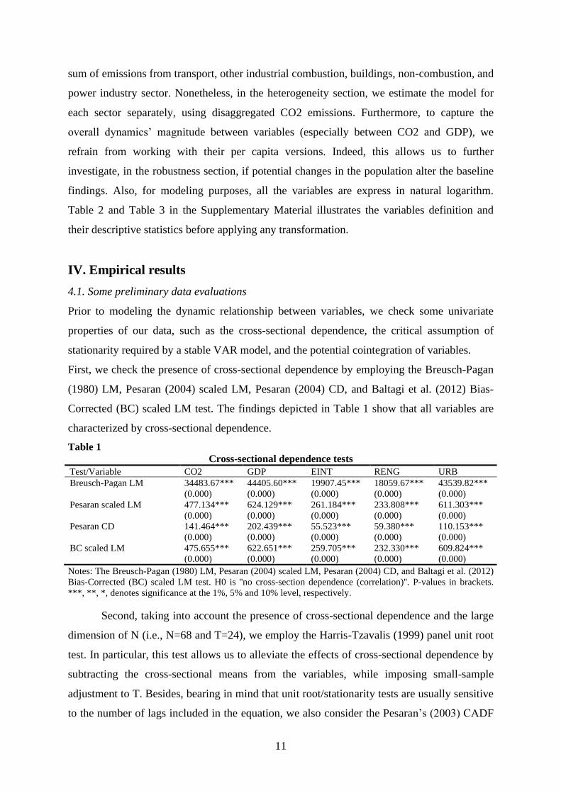
First, we check the presence of cross-sectional dependence by employing the Breusch-Pagan

(1980) LM, Pesaran (2004) scaled LM, Pesaran (2004) CD, and Baltagi et al. (2012) Bias-

Corrected (BC) scaled LM test. The findings depicted in Table 1 show that all variables are

characterized by cross-sectional dependence.

Table 1

Cross-sectional dependence tests

Test/Variable CO2 GDP EINT RENG URB

Breusch-Pagan LM 34483.67*** 44405.60*** 19907.45*** 18059.67*** 43539.82***

(0.000) (0.000) (0.000) (0.000) (0.000)

Pesaran scaled LM 477.134*** 624.129*** 261.184*** 233.808*** 611.303***

(0.000) (0.000) (0.000) (0.000) (0.000)

Pesaran CD 141.464*** 202.439*** 55.523*** 59.380*** 110.153***

(0.000) (0.000) (0.000) (0.000) (0.000)

BC scaled LM 475.655*** 622.651*** 259.705*** 232.330*** 609.824***

(0.000) (0.000) (0.000) (0.000) (0.000)

Notes: The Breusch-Pagan (1980) LM, Pesaran (2004) scaled LM, Pesaran (2004) CD, and Baltagi et al. (2012)

Bias-Corrected (BC) scaled LM test. H0 is ''no cross-section dependence (correlation)''. P-values in brackets.

***, **, *, denotes significance at the 1%, 5% and 10% level, respectively.

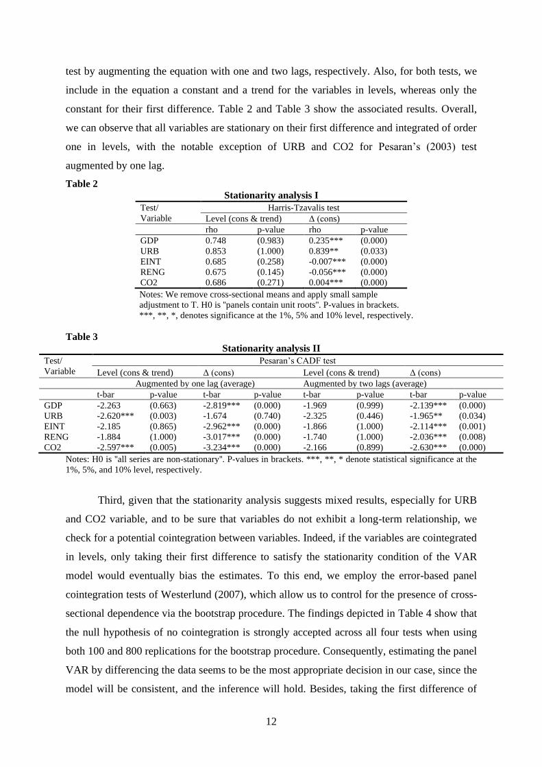
Second, taking into account the presence of cross-sectional dependence and the large

dimension of N (i.e., N=68 and T=24), we employ the Harris-Tzavalis (1999) panel unit root

test. In particular, this test allows us to alleviate the effects of cross-sectional dependence by

subtracting the cross-sectional means from the variables, while imposing small-sample

adjustment to T. Besides, bearing in mind that unit root/stationarity tests are usually sensitive

to the number of lags included in the equation, we also consider the Pesaran’s (2003) CADF

12

test by augmenting the equation with one and two lags, respectively. Also, for both tests, we

include in the equation a constant and a trend for the variables in levels, whereas only the

constant for their first difference. Table 2 and Table 3 show the associated results. Overall,

we can observe that all variables are stationary on their first difference and integrated of order

one in levels, with the notable exception of URB and CO2 for Pesaran’s (2003) test

augmented by one lag.

Table 2

Stationarity analysis I

Test/

Variable

Harris-Tzavalis test

Level (cons & trend) Δ (cons)

rho p-value rho p-value

GDP 0.748 (0.983) 0.235*** (0.000)

URB 0.853 (1.000) 0.839** (0.033)

EINT 0.685 (0.258) -0.007*** (0.000)

RENG 0.675 (0.145) -0.056*** (0.000)

CO2 0.686 (0.271) 0.004*** (0.000)

Notes: We remove cross-sectional means and apply small sample

adjustment to T. H0 is ''panels contain unit roots''. P-values in brackets.

***, **, *, denotes significance at the 1%, 5% and 10% level, respectively.

Table 3

Stationarity analysis II

Test/

Variable

Pesaran’s CADF test

Level (cons & trend) Δ (cons) Level (cons & trend) Δ (cons)

Augmented by one lag (average) Augmented by two lags (average)

t-bar p-value t-bar p-value t-bar p-value t-bar p-value

GDP -2.263 (0.663) -2.819*** (0.000) -1.969 (0.999) -2.139*** (0.000)

URB -2.620*** (0.003) -1.674 (0.740) -2.325 (0.446) -1.965** (0.034)

EINT -2.185 (0.865) -2.962*** (0.000) -1.866 (1.000) -2.114*** (0.001)

RENG -1.884 (1.000) -3.017*** (0.000) -1.740 (1.000) -2.036*** (0.008)

CO2 -2.597*** (0.005) -3.234*** (0.000) -2.166 (0.899) -2.630*** (0.000)

Notes: H0 is ''all series are non-stationary''. P-values in brackets. ***, **, * denote statistical significance at the

1%, 5%, and 10% level, respectively.

Third, given that the stationarity analysis suggests mixed results, especially for URB

and CO2 variable, and to be sure that variables do not exhibit a long-term relationship, we

check for a potential cointegration between variables. Indeed, if the variables are cointegrated

in levels, only taking their first difference to satisfy the stationarity condition of the VAR

model would eventually bias the estimates. To this end, we employ the error-based panel

cointegration tests of Westerlund (2007), which allow us to control for the presence of cross-

sectional dependence via the bootstrap procedure. The findings depicted in Table 4 show that

the null hypothesis of no cointegration is strongly accepted across all four tests when using

both 100 and 800 replications for the bootstrap procedure. Consequently, estimating the panel

VAR by differencing the data seems to be the most appropriate decision in our case, since the

model will be consistent, and the inference will hold. Besides, taking the first difference of

13

the log-transformed data facilitate the modeling between variables by allowing us to work

with their growth rates.

Table 4

Panel cointegration tests

Westerlund (2007)

Statistic Z-value Robust p-value Z-value Robust p-value

bootstrap with 100 replications bootstrap with 800 replications

Gt 0.669 0.271 0.669 0.271

Ga 13.271 1.000 13.271 1.000

Pt 10.714 0.591 10.714 0.591

Pa 9.670 0.684 9.670 0.684

Notes: H0 is ''no cointegration''. The equation includes the constant term, one lag, and one lead. The width

of the Bartlett kernel window is set to three. ***, **, *, denotes significance at the 1%, 5% and 10% level,

respectively.

4.2. Identification and estimation of the structural panel VAR model

4.2.1. Identification

A crucial aspect of the VAR approach involves the assumptions imposed to estimate the

associated system of simultaneous equations consistently. Indeed, converting the classical

VAR into a structural VAR (SVAR) approach by setting specific restrictions, allow us to

achieve the necessary causal inference, and have a meaningful economic interpretation of the

parameters. In other words, the identification in SVAR of all structural parameters requires

that some theory-based economic restrictions are imposed. In doing so, we draw upon a

recursive panel SVAR model, meaning that we do not impose any restriction on the matrix

that captures the impact effects8, i.e. we use exclusion restrictions. Effectively, this can be

done by imposing a particular causal order between variables, which plays a vital role in the

computation of both the Cholesky decomposition of the innovations' variance-covariance

matrix and the IRFs (Abrigo & Love, 2016). Correspondingly, we further detail the rationale

behind the causal ordering we impose on the systems’ variables.

First, according to the EKC hypothesis and STIRPAT framework, we argue that the

GDP exhibits the highest levels of exogeneity, while CO2 the highest level of endogeneity.

More specifically, we consider that CO2, namely the variable ordered last into our

transmission channel, responds more quickly following exogenous shocks to economic

activity. Thus, the exogenous structural disturbances to output have both a

contemporaneously and lagged impact on the CO2. Opposite, the GDP being ordered first

into the system may have only a delayed response to any exogenous shocks to CO2 (i.e. is

restricted to respond within the period).

8 The matrix of impact effects or impact multipliers matrix, stands for the matrix that contains the immediate

responses of the variables following a structural shock.

14

Second, the three remaining variables, namely the urbanization, energy intensity, and

renewable energy, enter the transmission channel at the right- (left) side of the GDP (CO2).

The reasoning for this choice is straightforward. On the one hand, as previously mentioned,

the related literature ranks these factors among the most important determinants of CO2

emission. On the other hand, regarding the sample’s particularities (discussed more is

detailed in the Introduction section), they may easily explain the ongoing urbanization

process, along with the efforts made by developing economies to combat climate change. In

this manner, for example, the active involvement in the CDM of the Kyoto Protocol may

mirror some of the countries’ efforts aiming to reduce environmental degradation. However,

what remains ambiguous so far, is the causal ordering of these factors in the transmission

channel, given that it may influence our results. Indeed, we may have less information than

the underlying economic foundation of CO2-GDP nexus, but the economic intuition could

equally help us in this regard.

Subsequently, we assume that any exogenous shocks to output may impact the

urbanization degree, which may further influence the energy intensity, renewable energy

share, and the CO2. The same logic is preserved for the other variables, namely the external

disturbances to energy intensity may affect renewables, which in turn may reflect on the CO2

emissions levels. Thus, the CO2 emissions are ultimately allowed to react within the period to

any exogenous shocks to the other system's variables. In contrast, all the variables respond

within the period following exogenous shocks to output.

Taken collectively, our previous economic rationale may be linked with the fast

growth of developing economies, which may impact the scale of the urbanization process. As

a result, we expect that the intensification of economic processes to increase the energy use,

but at the same time, at least from a sustainability perspective, to foster the advance in energy

efficiency and renewables. Notably, we postulate that efforts to promote energy efficiency

and the renewable energy share are a by-product of the pressures caused by urbanization and,

in any case, economic activity. Indeed, these efforts may also suggest the countries'

willingness to get involved in pollution mitigation activities.

Nonetheless, the Granger (1969) causality Wald test can also help us verify the

underlying economic reasoning. In this regard, we note that the associated results depicted in

Table 5 in the Supplementary Material overwhelmingly endorse the assumed transmission

channel between variables. Specifically, the findings show that each factor separately

Granger-causes the CO2 (except the renewable energy), while all four variables jointly

Granger-cause the CO2. Besides, GDP, along with all the excluded variables taken together,

15

Granger-cause the equation variable. Also, as a counterfactual, the causality towards the GDP

runs only from the renewable energy share, but its statistical significance is considerably low.

4.2.2. Estimation

A key primary step in estimating the panel SVAR involves setting the optimal lag length of

the model. Therefore, we choose the appropriate order of our panel SVAR, according to

moment and model selection criteria (MMSC) proposed by Andrews & Lu (2001) based on

Hansen’s (1982) J statistic. Table 6 in the Supplementary Material presents the associated

results. Overall, the MMSC statistics indicate that the first-order panel SVAR is the most

suitable, compared with the other two alternatives, namely the second- and third-order

specifications.9

Accordingly, we estimate the first-order panel SVAR model through the GMM

estimator. The results displayed in Table 8 in the Supplementary Material show the

following.10 On the one hand, the output has a significant positive one-lag impact on itself,

urbanization, and CO2, while a negative one on the energy intensity and renewable energy.

On the other hand, urbanization, renewable energy, and CO2 respond positively and

significantly to a one-lag impact of urbanization. Moreover, the energy intensity seems to

have a significant increasing delayed effect only on CO2 emissions. Also, given that

renewable energy displays a significant negative one-lag impact on GDP, there is a negative

feedback effect at work between the indicators.

The first-order panel SVAR-GMM findings give us an original resolution on the

dynamic behavior between variables. Indeed, it also represents the leading basis for the

crucial IRFs and forecast-error variance decompositions (FEVDs), which may be retrieved

following its multivariate estimation. As such, being mainly interested in the CO2 response

following shocks to other system variables, let us now discuss the associated orthogonalized

9 Along with MMSC (i.e. Bayesian, Akaike, and Hannan-Quinn information criterion) also the overall

coefficient of determination (CD) which shows the share of the variation explained by the model and Hansen’s

(1982) J statistic of over-identifying restrictions are reported (see Abrigo & Love, 2016). However, we rely

predominantly on MMSC in choosing the optimal lag length, given that the Hansen’s (1982) J statistic has no

correction for the degrees of freedom and, thus, may provide biased results. Also, we mention that the chosen

model accepts Hansen’s overidentification restriction at a 1% level of significance. 10 Post estimation, we examine the stability condition of the panel SVAR-GMM model. As such, we note that all

eigenvalues lie inside the unit root circle, proving that the model is correctly specified and exhibits a high

accuracy (see Table 7 and Figure 1 in the Supplementary Material).

16

cumulative IRFs11 and FEVDs, both generated based on 1000 Monte Carlo simulations, and

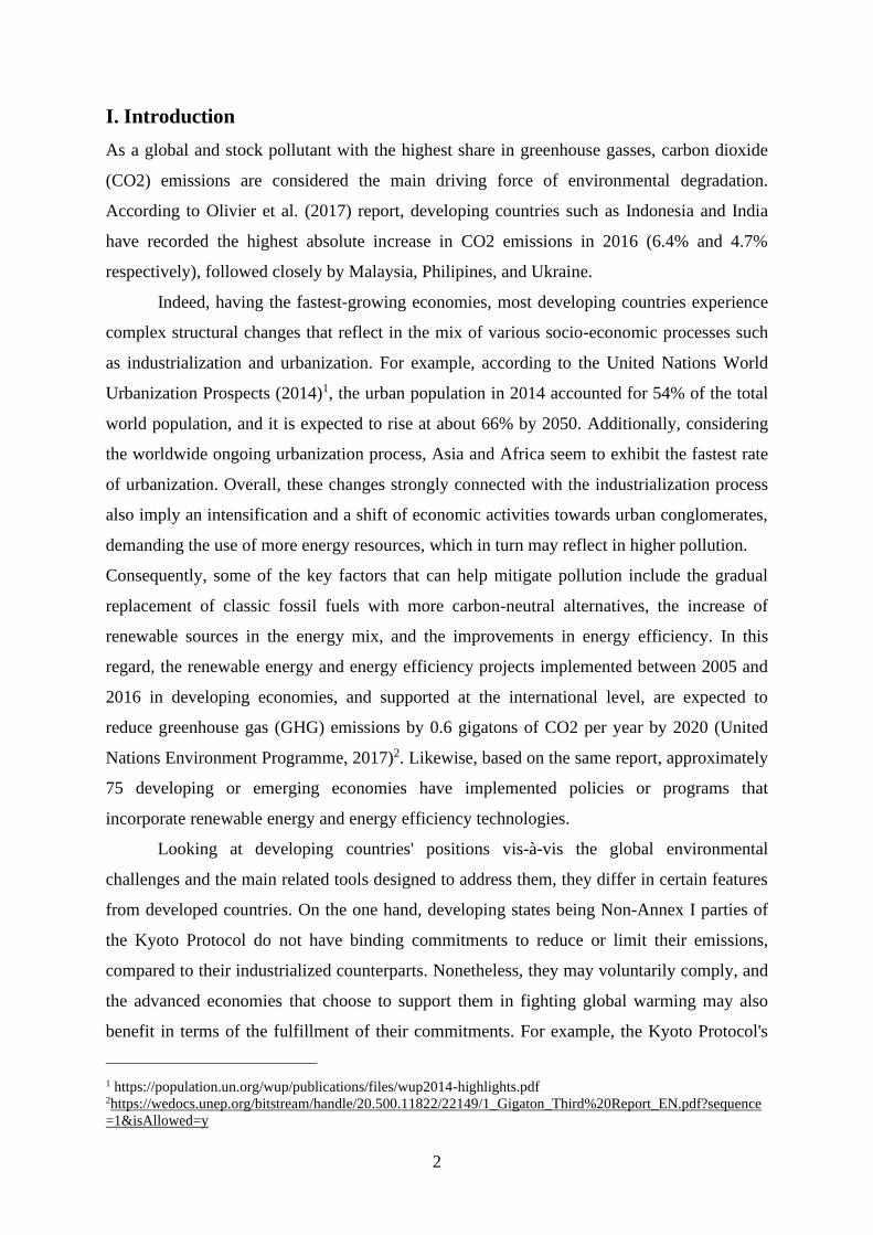
depicted in Figure 1 and Table 5, respectively.

First, the IRFs indicate that one standard deviation exogenous positive shock to GDP

triggers a persistent increase in CO2 emissions, both immediately and cumulated over the

twenty years horizon. More specifically, the CO2 increases with about two percentage points

(pp) on impact, following a positive shock to output. Although it shows a smooth evolution

over time, the upward trend seems to be slightly bent to the right. Likewise, its magnitude

almost triples in the long-run, reaching and even exceeding five pp. From an economic

perspective, these findings suggest that developing countries under examination are situated

on the EKC's growing side. However, depending on their economic context, the results may

suggest that they are likely to reach the crucial GDP turning point in the long-run sooner or

later. Overall, these findings are expected, considering that the developing countries exhibit

among the highest GDP growth rates, which are often incompatible with lower levels of

environmental pollution. For example, a positive exogenous technology shock may induce

the well-known phenomena of "catch-up growth" and, thus, trigger the intensification of

industrial processes, which would eventually reflect at first in higher pollution. Indeed, as the

nations' economic welfare grows, they can more easily acquire advanced green technologies,

which, along with the increase in household income, may equally promote environmental

sustainability. Thus, over time these may help in flattening the pollution curve. In this

fashion, judging from the perspective of a future potential validity of EKC, our findings may

complement the work of Liddle (2013), Shahbaz et al. (2015), Dogan & Seker (2016), Li et

al. (2016), Wang et al. (2016), Talbi (2017), Naminse & Zhuang (2018), Pata (2018), among

others.

Second, one standard deviation permanent positive shock to urbanization triggers an

increase in CO2, which may attain almost five pp after twenty years from impact. Also, we

note that the cumulated effect becomes statistically significant only after two years. This may

imply that the adverse effects of the urbanization process are not reflected immediately on the

environment, but rather with a delay. Additionally, the overall pattern of the CO2 response

seems to mirror to a certain extent the CO2 response to GDP shocks, suggesting that states

will be able to reach the urbanization threshold that would lead to a decrease in CO2 in the

future. In this regard, the results are similar to studies that unveil a bell-shaped pattern

11 We also recovered the simple orthogonalized IRFs, given that they are useful in evaluating the overall

stability of our model. In this regard, Figure 2 in the Supplementary Material shows that the CO2 responses

move towards zero over time, supporting both the variables’ stationarity condition and the overall stability of the

model.

17

between urbanization and environmental degradation (see e.g. Martínez-Zarzoso & Maruotti,

2011; Lin & Zhu, 2017; Chen et al., 2019).

Third, a positive one standard deviation shock to energy intensity raises the CO2 by

about three pp on impact. As well, the cumulate CO2 response exhibits a sharp increase over

roughly the first one year and a half, then stabilizes and very slowly increases until it reaches

nearly four pp following a permanent shock to energy intensity. This result is in line with the

study of Sadorsky (2014a), Shahbaz et al. (2015), and Naminse & Zhuang (2018), but

opposes the one of Martínez-Zarzoso & Maruotti (2011).

Fourth, in terms of the overall pattern displayed, the response of CO2 following a positive

exogenous shock to renewables seems quite similar to the cumulate effect produced by an

exogenous shock to energy intensity. However, one standard deviation positive shock to

RENG induces an opposite effect, namely a decrease of about two pp in CO2 at the moment

of the impact. Moreover, the cumulate magnitude of the negative response diminishes

significantly after the initial impact, and then stabilize and gravitate around the same value

for the rest of the period. We note that the permanent shock, projected twenty years ahead,

still causes a drop in CO2, even if the magnitude is slightly lower (i.e. around one and a half

pp). These findings corroborate the ones of López-Menéndez et al. (2014), Dogan & Seker

(2016), and Charfeddine & Kahia (2020) while contrasting those of Bölük & Mert (2014).

Finally, the CO2 increases at about nine pp in the aftermath of a permanent exogenous

positive shock to itself. However, the increasing of the cumulative response in the long-run is

almost imperceptible, pointing out a low magnitude of CO2 persistence (see the top-left plot

in Figure 1). Overall, this finding supports the one of Martínez-Zarzoso & Maruotti (2011),

Sadorsky (2014a), and Acheampong (2018), among others, who find persistence effects in

CO2 emissions.

Concerning FEVDs, on the one hand, as expected, the largest share of the variables'

variation is explained by their dynamics (see the principal diagonal of Table 3). Furthermore,

energy intensity seems to explain, twenty years ahead, about 9.99% of the variation in CO2,

followed by renewable energy (4.06%), output (3.99%), and urbanization (2.01%). Indeed,

the findings seem to uphold the energy as the primary contributor of CO2 in our group of

developing economies. Also, the results indicate that the renewables have a more significant

long-term contribution to CO2, compared to output and urbanization. Overall, this is a quite

exciting and promising result, which may suggest, yet again, that these states have made

substantial efforts to switch towards more environmentally friendly energy sources, and,

among others, that the CDM related projects have had the desired outcomes. Likewise, this

18

result is also supported by the large share of renewable energy variation, following a shock to

energy intensity.

On the other hand, we remark that the external shocks to output explain, twenty years

ahead, a large share of variation in the other macro factors. These findings are also not

unexpected, considering that the exogenous disturbances propagate first through output an

then to its related macro components. Besides, it seems that any exogenous shocks to the

remaining column variables, do not exhibit a large magnitude in explaining the fluctuations in

the row variables.

Figure 1

Cumulative orthogonalized IRFs

Observations: 1428 • Groups: 68

Notes: Considering two generic variables A and B, “A: B” denotes the response of B following

shocks to A. The continuous line denotes the impulse response functions. The dashed lines

stand for the associated 95% confidence interval computed based on 1000 Monte Carlo

simulations.

19

Table 5

Twenty years horizon forecast-error variance decompositions

Response variables Impluse variables

GDP URB EINT RENG CO2

GDP 99.36 0.21 0.19 0.19 0.02

URB 12.31 87.54 0.02 0.01 0.09

EINT 21.59 0.14 78.14 0.04 0.07

RENG 0.89 0.37 8.17 90.47 0.08

CO2 3.99 2.01 9.99 4.06 79.92

Notes: The numbers (in percentages) show the variation in the row variable that is explained by

the column variables.

V. Robustness

We assess the robustness of our baseline SVAR specification in several ways. Also, we focus

on reporting the associated findings with respect to the crucial IRFs, retrieved after running

the panel SVAR-GMM model.

5.1. Alternative ordering

Considering that we use a recursive ordering strategy to achieve identification in our SVAR,

we check the stability of the underlying economic rationale by implementing alternative

transmission schemes. On the one hand, we check the soundness of our economic intuition

behind the ordering of the factors positioned at the right-side (left-side) of GDP (CO2) within

the transmission scheme, namely URB, EINT, and RENG. In this manner, we switch their

initial position by running a five-time rotation between them, until we consider all available

options. On the other hand, we order each of these three factors at the top of the transmission

channel, namely before the output. Therefore, we can observe if changing the variable which

exhibits the highest level of exogeneity alters the baseline findings. It should be mentioned

that these new restrictions imposed among the system variables are even more consistent with

the literature that positions urbanization, energy intensity, and renewables as the main

determinants of CO2.

As shown by Figure 3 in the Supplementary Material, using distinct ordering

scenarios does not qualitatively alter the baseline findings. Indeed, as expected, small

changes in the magnitude of the responses are present. In this fashion, we note that a more

visible difference is at work for CO2 response following external shocks to EINT, especially

in the model where EINT is ordered first into the transmission channel. In particular, the

cumulative response of CO2 due to a positive shock to EINT seems to follow a downward

trend after reaching the peak, that is, approximately after one year and a half after the impact.

One possible explanation could be related to the fact that manifesting the highest level of

20

exogeneity, the effect of energy intensity on CO2, does not also include the effect of

disturbances to GDP and urbanization. As such, the energy intensity may appear much lower,

thus, having a lower impact on CO2.

5.2. Altering the sample

To check whether our baseline findings are robust under certain economic or political distress

conditions, we account for some well-known related events which can be seen in relation to

both T and N dimensions of our sample. First, to control for the potential (delayed) effects of

the global financial crisis, we restrict the period of analysis to (1992-2010) 1992-2008.

Furthermore, the exclusion of the period following 2008 coincides with the starting point of

the Kyoto Protocol's first commitment phase (i.e. 2008-2012). Thus, if there were specific

changes in the environmental behavior of developed countries as a result of potential

pressures to achieve their binding targets, we would expect them to reflect on developing

countries as well. Second, we drop the period immediately following the end of the Cold

War, namely 1992-1996, since the economies affected by this quite prominent geopolitical

distress could have encountered difficulties in terms of economic recovery. Indeed, if our

assumption hold, the fluctuations in their primary macro aggregates may alter the baseline

findings. Third, having in mind the Arab Spring, which involves several developing states,

we also check whether its effects reflected on our results. In doing so, we drop from the

sample all the economies affected to some extend by this major political unrest episode.

Finally, it is generally recognized that the petroleum industry has major implications on the

environment. In this fashion we exclude all states ranked by the Central Intelligence Agency

(CIA)12 among the top thirty economies regarding the crude oil exports. Overall, the

associated cumulative IFRs, depicted in Figure 4 in the Supplementary Material, shows that

independent of the restriction imposed on the sample, the baseline results are preserved both

in terms of pattern and statistical significance.

5.3. Exogenous control factors

We exogenously introduce, along with the main SVAR endogenous variables, several

additional explanatory factors into the model to control for a potential bias caused by omitted

variables. These variables are related to changes in the size of the economy13 (population),

12 For more details, see https://www.cia.gov/library/publications/the-world-factbook/fields/262rank.html 13 With respect to possible changes in countries’ population, we estimate two alternative models using (i) GDP

and CO2 in per capita terms, and (ii) GDP, EINT, and CO2 in per capita terms (i.e. their growth rates in per

21

sectoral output composition (agriculture, industry, and services as % of GDP), trade (trade as

% of GDP), environmental prospects (forest rents as % of GDP), external financing

(remittances in % GDP), and private sector financial conditions (domestic credit to the

private sector as % GDP) (see Table 2 and Table 3 in the Supplementary Material for

variables definition and descriptive statistics, respectively). Also, to maintain the stability

conditions of the SVAR model and consistency between variables, we transformed them into

growth rates, by taking the first difference of their log-transformed values. Overall, the

cumulative IRFs illustrated by Figure 5 in the Supplementary Material indicate that the

findings are comparable with those of the baseline model, especially judging based on the

significance and long-term trajectory of CO2 response due to different innovations shocks.

IV. Heterogeneity

This section explores the sensitivity of CO2 responses following external shocks to other

factors, depending on the income level group and the ratification or ascension date of states to

the Kyoto Protocol.

6.1. The level of economic development

The economic development stages that a country crosses imply that different effects such as

scale, structural, or technological, are at work during different periods and may cause

substantial fluctuations in environmental conditions (see e.g. Grossman & Krueger, 1991).

Thus, to explore the possible difference of CO2 responses with respect to countries’ income

level, we construct two sub-samples of low and lower-middle income economies, based on

the World Bank classification (2017) (see Table 4 in the Supplementary Material for

summary statistics). Panel (a) and panel (b) in Figure 6 in the Supplementary Material depicts

the cumulative IRFs for both income sub-samples. First, as expected, following external

shocks, the GDP exhibits a positive effect on CO2 but with higher magnitude in lower-

middle income economies. Moreover, the cumulated CO2 response over the first two years

displays a sharp increase in lower-middle income states, compared to the low income ones.

Likewise, the increasing long-run trajectory seems to be more accentuated in wealthier

countries.

capita terms, computed as the difference of log-transformed values). As shown by the panel (e)-(f) in Figure 4 in

the Supplementary Material, the cumulative IRFs are almost identical to those revealed by the baseline model.

22

Second, CO2 emissions significantly and positively react due to innovations shocks to

urbanization only in low income countries, and with a delay of around four years. Besides,

the CO2 response path tends to display a bell-shaped pattern in the long-term, supporting the

urbanization-EKC hypothesis. Conversely, the lack of significance in the lower-middle

income countries may suggest that the urbanization process is at a more advanced stage,

leading to a more abundant flow of sophisticated ecological practices that help in combating

pollution.

Third, following a positive shock to energy intensity (renewables), the CO2 emissions

respond in a positive (negative) way in both income groups. As well, the cumulated effect

shows a sharp increase after the impact in both sub-samples (except CO2 response following

renewables shocks in low income states, where the increase seems to be smoother and lower

in magnitude). However, starting approximately with the second year, the IRFs indicate that

the cumulated effect stabilizes and preserves its positive linear trajectory up to twenty years

in low income states. In contrast, it follows a monotonically increasing pattern in lower-

middle income ones. On the whole, this may confirm that in countries where the

industrialization process is more pronounced, it also becomes more challenging to maintain

low levels of pollution.

Finally, an exogenous positive shock to CO2 leads to an increase in its levels, and the

magnitude of impact seems to be comparable in both groups. Nonetheless, in low income

countries, the cumulated response starts to decline after the impact, and then quickly readjust

(after about two years) to a linear path that remains stable in the long-run. Opposite, in lower-

middle income economies, the cumulated response keeps an increasing trajectory over the

twenty years horizon.

6.2. The Kyoto Protocol status

We split the main sample taking into account the date of the ratification/accession of

individual states to the Kyoto Protocol based on the United Nations Treaty Collection14.

Thus, the first sub-sample (Kyoto Protocol group A) comprises the nations which ratified or

acceded before the year in which it entered into force (i.e. 2005), while in the second group

(Kyoto Protocol group B) we include the remaining countries for which the

ratification/accession date is 2005 onwards (see Table 4 in the Supplementary Material for

14https://treaties.un.org/Pages/ViewDetails.aspx?src=TREATY&mtdsg_no=XXVII-7-

a&chapter=27&clang=_en.

23

summary statistics). The cumulative IRFs are illustrated by panels (c) and (d) in Figure 6 in

the Supplementary Material.

On the one hand, the findings indicate that for the states which ratified or acceded to

the Kyoto Protocol before 2005, the evolution of cumulated CO2 response following output

and urbanization shocks seems to switch its increasing trend in the long-run. In particular,

this suggests that this group of countries may attain the peak in CO2 more rapidly and for

lower levels of GDP and URB, compared to the economies which ratified /acceded to the

Protocol after it entered into force. As such, the traditional and urbanization-EKC hypothesis

seems to be more realistic for the Kyoto Protocol group A. Moreover, for the Kyoto Protocol

group A states, the urbanization exhibits a delayed cumulated effect on CO2. In contrast, for

the members of group B, the effect loses its significance in the long-term.

On the other hand, an exogenous increase in energy intensity (renewables) triggers a

cumulated positive (negative) effect on CO2 in both groups of economies. However, at the

moment of the impact, the magnitude of CO2 response is higher due to energy intensity

(renewable energy) disturbances for the states which ratified/acceded to the Kyoto Protocol

before (after) it entered into force. Also, in the next two years after the impact, the cumulated

magnitude of CO2 response following both energy intensity and renewables shocks increases

sharply, but then stabilizes and raises very slowly for the group A economies. For the group

B states, the cumulated response of CO2 (i) raises abruptly after the impact due to EINT

disturbances, but then stabilizes to a new high and follows a linear path until the end of the

period, (ii) remains roughly at the same level recorded at the time of the impact following

renewable energy shocks. Besides, a positive one standard deviation shock to CO2 has a

positive effect on its levels for both groups. However, the cumulated effect increases

(decreases) slowly over the years across the states of the Kyoto Protocol group A (B).

Overall, the findings may suggest that the states which ratified or acceded to the Protocol

before 2005 are the ones that have undergone significant changes in their economic

development (e.g. have experienced a more intense process of industrialization and

urbanization, among others). Thus, they were committing much faster in actions to counteract

the potential adverse effects on the environment.

24

VII. Sectoral CO2 emissions

To have a more in-depth look at the potential changes in pollution dynamics in the

relationship with our macro indicators, we substitute aggregated CO2 with its sector-specific

counterparts (see Table 2 and Table 3 in the Supplementary Material for variables definition

and summary statistics, respectively).15 In doing so, we estimate the GMM-SVAR model

considering the CO2 related to each of the following sectors: transport, buildings, other

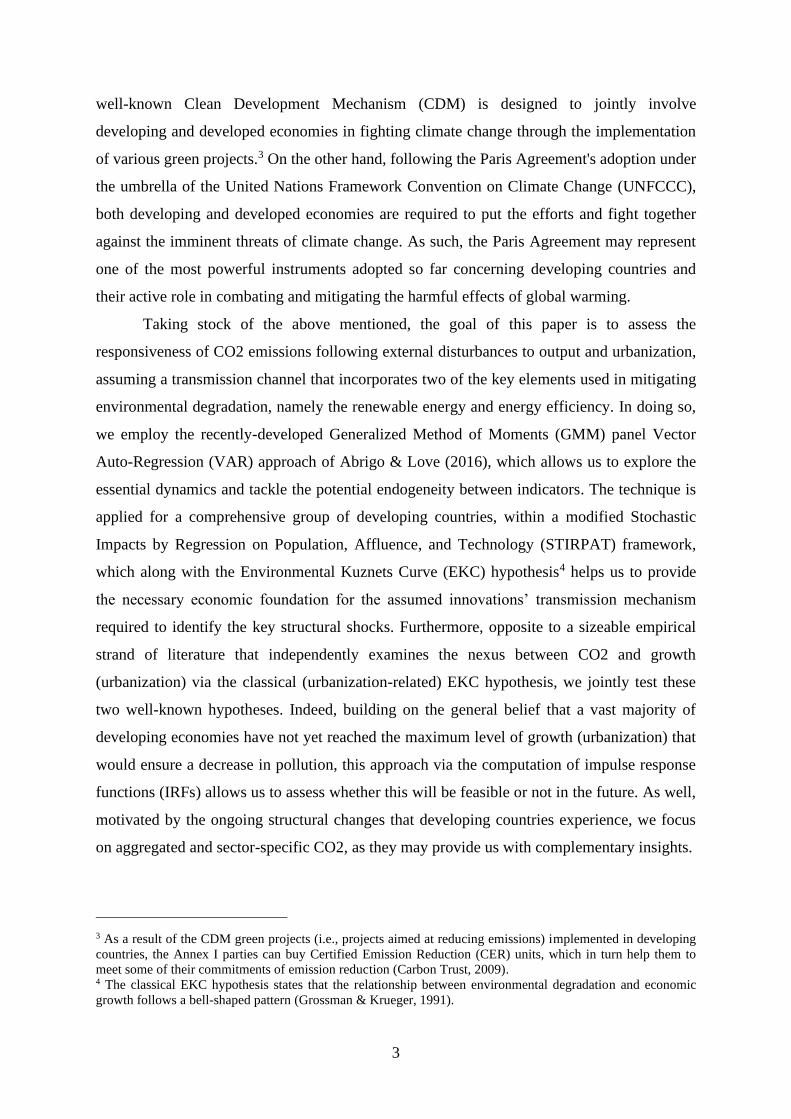
industrial combustion, non-combustion, and power industry. Figure 2 displays the CO2

sector-specific cumulative orthogonalized IRFs.

First, considering the presumed differences in the magnitude, an external shock to

output and urbanization has a cumulative significant positive effect on CO2 from transport,

buildings, and non-combustion sector—with the notable exception of CO2 from buildings

which do not significantly respond to urbanization disturbances. Besides, the significant

positive cumulated paths over the twenty-year horizon suggest that the related EKC

hypothesis may be at work in the very long-run, both for output and urbanization. Also, in

line with the baseline findings, the CO2 emissions respond with a delay of about two years

following urbanization shocks. On this last point, given that the construction industry has a

substantial contribution to the urbanization process, the lack of significance of the buildings-

related CO2 response following external shocks to urbanization may indicate that a

substantial number of green projects are implemented in this sector, thus, helping to reduce

the associated pollution.

Second, an exogenous increase in output and urbanization reduce the CO2 from other

industrial combustion and power industry sector both on impact and cumulated over twenty

years. However, industrial combustion- and power industry-related CO2 emissions do not

respond immediately to output shocks, but rather with roughly ten and eighteen years of

delay. Moreover, regarding the disturbances to urbanization, they seem to cause a U-shaped

pattern in cumulative CO2 emissions’ evolution, opposite to the bell-shaped pattern

postulated by the traditional EKC hypothesis.

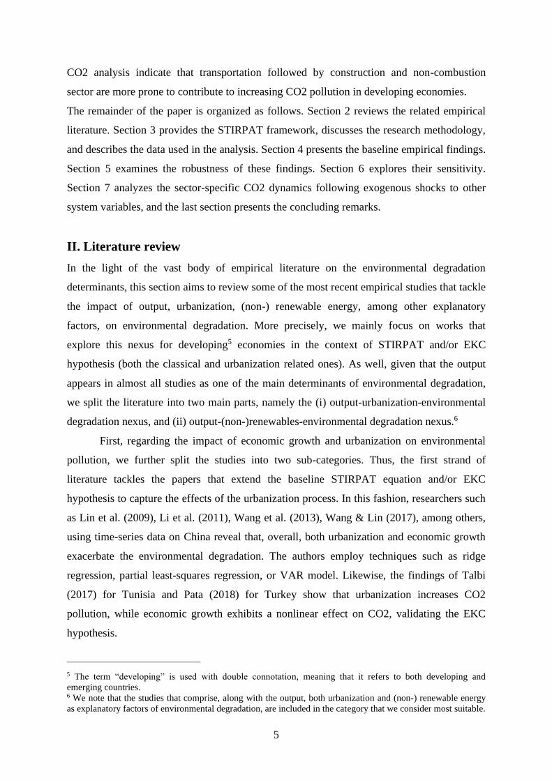
Third, the CO2 related to each of the five sectors react positively (negatively) to one

standard deviation energy intensity (renewables) shocks, both on impact and cumulated over

the twenty years, thus, backing up the baseline findings. However, the effect of renewables

15 We test the cross-sectional dependence and stationary properties of CO2 sector variables using the same tests

as for the baseline model. The findings confirm the presence of cross-sectional dependence, while the unit root

test shows that variables are stationary in levels (see Supplementary Material Table 9-11). However, in

empirical analysis, we use the first difference of the variables in order to work with growth rates and have all the

variables in the system at the same level.

25

on CO2 from non-combustion and power industry is not statistically significant. Indeed, these

two similar results may go hand in hand, given that access to energy in developing countries

is a significant issue, mainly alleviated, among others, by the transition to off-grid renewable

energy systems [International Renewable Energy Agency (IRENA), 2015). More precisely,

the off-grid renewables technologies (e.g. solar, micro-hydro, wind, biomass, among others),

whose leading market is concentrated in developing economies, represent the more

environmentally-friendly and cost-effective alternative to classical non-renewable energy

sources, such as the fossil fuels used for electricity generation via combustion processes [see

e.g. IRENA, 2015; Renewable Energy Policy Network for the 21st Century (REN21), 2015].

Additionally, the results also corroborate with the negative effect of output and urbanization

on power industry-related CO2.

Fourth, an external increase in the sector-specific CO2 emissions triggers a

statistically significant increase in its levels. At the same time, the magnitude at the moment

of impact ranges from about 14.5 pp (CO2 from transport) to 30 pp (CO2 from other

industrial combustion). Furthermore, the cumulated effect starts to decay immediately after

the impact (except CO2 associated with other industrial combustion), and then quickly

stabilizes and follows an almost linear path until the end of the analyzed period. In particular,

the results may highlight, yet again, the inertial behavior of CO2 pollution levels.

Overall, the findings illustrate, on the one hand, the complexity of the relationship

between sector-specific CO2 and the several related key economic aggregates, highlighting

which sector is more likely to be associated in the future with higher pollution levels. On the

other hand, the results strengthen the vital role of non-combustion energy sources and energy

efficiency projects (e.g. the rapidly growing off-grid renewable systems, the use of

sustainable technologies in the construction industry, among many others) in promoting green

growth and urbanization, and ultimately in reducing the environmental degradation.

26

Figure 2

Cumulative orthogonalized IRFs: sectoral CO2 emissions (a) CO2 from transport (b) CO2 from buildings

Observations: 1428 • Groups: 68 Observations: 1428 • Groups: 67

(c) CO2 from other industrial combustion (d) CO2 from non-combustion

Observations: 1405 • Groups: 67 Observations: 1428 • Groups: 68

27

Figure 2

(continued) (e) CO2 from power industry

Observations: 1422 • Groups: 68

Notes: The continuous line denotes the impulse response functions. The dashed lines stand for the associated

95% confidence interval computed based on 1000 Monte Carlo simulations.

VIII. Conclusion and policy implications

This paper explored the impact of external changes in output, urbanization, energy intensity,

and renewable energy on aggregated and sector-specific CO2, within a modified STIRPAT

analytical framework. To this end, motivated by the potential endogenous behavior between

variables, we employed the novel panel GMM-VAR technique for a rich sample of 68

developing states over 1992-2015.

The results showed, on the one hand, that an exogenous increase in output,

urbanization, energy intensity and CO2 led to a significant increase in CO2, both on impact

and cumulated over the twenty years horizon. Besides, the CO2 response following

disturbances to output and urbanization, suggest that a threshold effect, compatible with the

classical and urbanization EKC hypothesis, might be at work in the long-run for our group of

countries. Conversely, we found that a positive shock to renewables cumulatively and

significantly decreases the current and future levels of CO2. In sum, these findings may

imply that in the context of rapid industrialization and urbanization, renewable energy is one

of the most powerful tools in mitigating environmental degradation. Nonetheless, more

considerable attention must also be paid to energy efficiency, especially as increasing it can

further enhance the beneficial effects of renewable energy on the environment. These results

are supported by several robustness tests, including an alternative Cholesky ordering of

variables, when altering the sample, and controlling for a series of exogenous factors. On the

other hand, the findings are found to be are sensitive concerning both countries’ level of

28

development and their Kyoto Protocol ratification/ascension status. Besides, the

disaggregated CO2 analysis unveiled essential differences regarding the contribution of

various sectors to the overall CO2 pollution. In particular, the results may suggest that the

CO2 emissions related to transportation, construction, and non-combustion sector are more

likely to increase in the future, compared to other industrial combustion and power industry

sector.

The findings could be transposed in some valuable policy recommendations. First,

developing countries should pay more attention to the implications that the process of

urbanization, as well as the growth-promoting policies, have on CO2 pollution. Moreover, the

urban planning and development policy requires an appropriate design to accommodate better

any potential negative impacts on the quality of the environment. Second, although countries

make outstanding efforts to invest as much as possible in renewable energy sources and

minimize energy dependency, these investments should be continuously adapted to cope with

the dynamics of their particular economic environment. Likewise, adequate monitoring

during project implementation may increase their efficiency and signal beforehand any

potential nonconformities. Third, to counterbalance and mitigate the overall pollution,

additional efforts should be directed towards the sectors where CO2 emissions are more

likely to increase. Finally, the ongoing international cooperation and assistance from

developed nations may represent a central pillar in ensuring environmental sustainability in

developing economies. Future work could consider a more detailed breakdown of energy

sources in assessing their impact on CO2 (see e.g. Antonakakis et al., 2017; Naminse &

Zhuang, 2018). However, this is strictly conditioned by data availability, especially for this

group of developing economies. As well, an analysis of the impact of various types of crises

on CO2, by making use of complementary techniques such as the local projection method

(see e.g. Jalles, 2019), could provide additional insights regarding the future behavior of CO2

emissions.

29

References

Abrigo, M.R.M. and Love, I., 2016. Estimation of Panel Vector Autoregression in Stata.

The Stata Journal, 16(3), pp.778-804.

Aldea, A., Ciobanu, A. and Stancu, I., 2012. The Renewable Energy Development: A

Nonparametric Efficiency Analysis. Romanian Journal of Economic Forecasting,

15(1), pp.5-19.

Andrews, D.W.K. and Lu, B., 2001. Consistent model and moment selection procedures

for GMM estimation with application to dynamic panel data models. Journal of

Econometrics, 101, pp.123-164.

Antonakakis, N., Chatziantoniou, I. and Filis, G., 2017. Energy consumption, CO2

emissions, and economic growth: An ethical dilemma. Renewable and Sustainable

Energy Reviews, 68, pp.808-824.

Apergis, N. And Payne, J.E., 2015. Renewable Energy, Output, Carbon Dioxide

Emissions, and Oil Prices: Evidence from South America. Energy Sources, Part B:

Economics, Planning, and Policy, 10(3), pp.281-287.

Arellano, M. and Bover, O., 1995. Another look at the instrumental variable estimation of

error-components models. Journal of Econometrics, 68(1), pp.29-51.

Awad, A. and Warsame, M.H., 2017. Climate Changes in Africa: Does Economic Growth

Matter? A Semi-parametric Approach. International Journal of Energy Economics

and Policy, 7, pp.1-8.

Bakirtas, T. and Akpolat, A.G., 2018. The relationship between energy consumption,

urbanization, and economic growth in new emerging-market countries. Energy, 147,

pp.110-121.

Baltagi, B.H., Feng, Q. and Kao, C., 2012. A Lagrange Multiplier test for cross-sectional

dependence in a fixed effects panel data model. Journal of Econometrics, 170,

pp.164-177.

Breusch, T.S. and Pagan, A.R., 1980. The Lagrange multiplier test and its applications to

model specification in econometrics. Review of Economic Studies, 47, pp.239-253.

Brückner, M., 2012. Economic growth, size of the agricultural sector, and urbanization in

Africa. Journal of Urban Economics, 71(1), pp.26-36.

Carbon Trust, 2009. Global Carbon Mechanisms: Emerging lessons and implications

(CTC748). Available at: <https://prod-drupal

files.storage.googleapis.com/documents/resource/public/Global%20Carbon%20Mech

anisms%20-%20Emerging%20Lessons%20And%20Implications%20-

%20REPORT.pdf> [Accessed on April 2020]

Central Intelligence Agency, 2020. The World Factbook, Country comparison: crude oil-

Exports. Available at: <https://www.cia.gov/library/publications/the-world-

factbook/fields/262rank.html> [Accessed on April 2020]

Charfeddine, L. and Kahia, M., 2019. Impact of renewable energy consumption and

financial development on CO2 emissions and economic growth in the MENA region:

A panel vector autoregressive (PVAR) analysis. Renewable Energy, 139, pp.198-213.

Chen, S., Jin, H. and Lu, Y., 2019. Impact of urbanization on CO2 emissions and energy

consumption structure: a panel data analysis for Chinese prefecture-level cities.

Structural Change and Economic Dynamics, 49, pp.107-119.

Dietz, T. and Rosa, E.A., 1994. Rethinking the environmental impact of population,

affluence and technology. Human Ecology Review, 1, pp.277-300.

Dietz, T. And Rosa, E.A., 1997. Effects of population and affluence on CO2 emissions.

Proceedings of the National Academy of Sciences, USA, 94(1), pp.175-179.

30

Doğan, B. and Değer, O., 2018. The Energy Consumption and Economic Growth in the E7

Countries: Cointegration in Panel Data with Structural Breaks. Romanian Journal of

Economic Forecasting, 21(1), pp.63-75.

Dogan, E. and Seker, F., 2016. Determinants of CO2 emissions in the European Union:

The role of renewable and non-renewable energy. Renewable Energy, 94, pp.429-439.

Ehrlich, P.R. and Holdren, J.P., 1971. Impact of population growth. Science, 171, pp.1212-

1217.

Gökgöz, F. and Güvercin, M.T., 2018. Energy security and renewable energy efficiency in

EU. Renewable and Sustainable Energy Reviews, 96, pp.226-239.

Granger, C.W.J., 1969. Investigating causal relations by econometric models and

cross-spectral methods. Econometrica, 37, pp.424-438.

Grossman, G.M. and Krueger, A.B., 1991. Environmental impacts of a North American free

trade agreement, NBER Working Paper No. 3914.

Hansen, L.P., 1982. Large sample properties of generalized method of moments

estimators. Econometrica, 50, pp.1029-1054.

Harris, R.D.F. and Tzavalis, E., 1999. Inference for unit roots in dynamic panels where the

time dimension is fixed. Journal of Econometrics, 91, pp.201-226.

Holtz-Eakin, D., Newey, W. and Rosen, H.S., 1988. Estimating vector autoregressions with

panel data. Econometrica, 56(6), pp.1371-1395.

Inglesi-Lotz, R. and Dogan, E., 2018. The role of renewable versus non-renewable energy

to the level of CO 2 emissions a panel analysis of sub- Saharan Africa’s Βig 10

electricity generators. Renewable Energy, 123, pp.36-43.

International Renewable Energy Agency, 2015. Off-grid renewable energy systems: status

and methodological issues, Working paper. Available at: <https://www.irena.org/-

/media/Files/IRENA/Agency/Publication/2015/IRENA_Off-

grid_Renewable_Systems_WP_2015.pdf> [Accessed on April 2020]

Iwata, H., Okada, K. and Samreth, S., 2011. A note on the environmental Kuznets curve

for CO2: a pooled mean group approach. Applied Energy, 88, pp.1986-1996.

Janssens-Maenhout, G., Crippa, M., Guizzardi, D., Muntean, M., Schaaf, E., Olivier,

J.G.J., Peters, J.A.H.W. and Schure, K.M., 2017. Fossil CO2 and GHG emissions of

all world countries. EUR 28766 EN, Publications Office of the European Union,

Luxembourg, 2017, ISBN 978-92-79-73207-2, doi:10.2760/709792.

Jebali, E., Essid, H. And Khraief, N., 2017. The analysis of energy efficiency of the

Mediterranean countries: A two-stage double bootstrap DEA approach. Energy, 134,

pp.991-1000.

Joshi, P. and Beck, K., 2018. Democracy and carbon dioxide emissions: Assessing the

interactions of political and economic freedom and the environmental Kuznets curve.

Energy Research & Social Science, 39, pp.46-54.

Kaya, Y., 1990. Impact of Carbon Dioxide Emission Control on GNP Growth: Interpretation

of Proposed Scenarios. Paris: IPCC Energy and Industry Subgroup, Response

Strategies Working Group.

Kurniawan, R. and Managi, S., 2018. Coal consumption, urbanization, and trade openness

linkage in Indonesia. Energy Policy, 121, pp.576-583.

Li, T., Wang, Y. and Zhao, D., 2016. Environmental Kuznets Curve in China: New

evidence from dynamic panel analysis. Energy Policy, 91, pp.138-147.

Li, H., Mu, H., Zhang, M. and Li, N., 2011. Analysis on influence factors of China’s CO2

emissions based on Path–STIRPAT model. Energy Policy, 39, pp.6906-6911.

Liddle, B., 2013. Population, affluence, and environmental impact across development:

Evidence from panel cointegration modeling. Environmental Modelling & Software,

40, pp.255-266.

31

Lin, B. and Zhu, J., 2017. Energy and carbon intensity in China during the urbanization and

industrialization process: A panel VAR approach. Journal of Cleaner Production

Volume 168, pp.780-790.

Lin, S., Zhao, D. And Marinova, D., 2009. Analysis of the environmental impact of China

based on STIRPAT model. Environmental Impact Assessment Review, 29, pp.341-

347.

Liu, W.-C., 2013. The Relationship between Energy Consumption and Output: A

Frequency Domain Approach. Romanian Journal of Economic Forecasting, 16(4),

pp.44-55.

López-Menéndez, A.J., Pérez, R. and Moreno, B., 2014. Environmental costs and

renewable energy: Re-visiting the Environmental Kuznets Curve. Journal of

Environmental Management, 145, pp.368-373.

Love, I. and Zicchino, L., 2006. Financial development and dynamic investment behavior:

evidence from panel VAR. The Quarterly Review of Economics and Finance, 46(2),

pp.190-210.

Martínez-Zarzoso, I. and Maruotti, A., 2011. The impact of urbanization on CO2 emissions:

Evidence from developing countries. Ecological Economics, 70(7), pp.1344-1353.

Martínez-Zarzoso, I., Bengochea-Morancho, A. and Morales-Lage, R., 2007. The impact of

population on CO2 emissions: evidence from European countries. Environmental and

Resource Economics, 38, pp.497512.

Naminse, E.Y. and Zhuang, J., 2018. Economic Growth, Energy Intensity, and Carbon

Dioxide Emissions in China. Polish Journal of Environmental Studies, 27(5),

pp.2193-2201.

Nickell, S., 1981. Biases in Dynamic Models with Fixed Effects. Econometrica, 49(6),

pp.1417-1426.

Olivier, J.G.J., Janssens-Maenhout, K.M, Schure, M., & Peters J.A.H.W. (2017). Trends in

global CO2 and total greenhouse gas emissions: 2017 report. PBL Netherlands

Environmental Assessment Agency, The Hague. Available at:

<https://www.pbl.nl/sites/default/files/cms/publicaties/pbl-2017-trends-in-global-co2-

and-total-greenhouse-gas-emissons-2017-report_2674.pdf> [Accessed on June 2019].

Pata, U.K., 2018. Renewable energy consumption, urbanization, financial development,

income and CO 2 emissions in Turkey: Testing EKC hypothesis with structural

breaks. Journal of Cleaner Production, 187, pp.770-779.

Pesaran, H., 2003. A simple panel unit root test in the presence of cross section

dependence, Cambridge WP in Economics, no. 0346, University of Cambridge.

Pesaran, H., 2004. General diagnostic tests for cross section dependence in panels,

Cambridge Working Paper in Economics No. 0435, University of Cambridge.

Poumanyvong, P. and Kaneko, S., 2010. Does urbanization lead to less energy use and

lower CO2 emissions? A cross-country analysis. Ecological Economics, 70, pp.434-

444.

Renewable Energy Policy Network for the 21st Century, 2015. Renewables Global Status

Report - Annual reporting on renewables: Ten years of excellence. Available at:

<https://www.ren21.net/wp-content/uploads/2019/05/GSR2015_Full-

Report_English.pdf> [Accessed on April 2020]

Sadorsky, P., 2014a. The effect of urbanization on CO2 emissions in emerging economies.

Energy Economics, 41, pp.147-153.

Sadorsky, P., 2014b. The Effect of Urbanization and Industrialization on Energy Use in

Emerging Economies: Implications for Sustainable Development. American Journal

of Economics and Sociology, 73(2), pp.392-409.

32

Sadorsky, P., 2009. Renewable energy consumption and income in emerging economies.

Energy Policy, 37(10), pp.4021-4028.

Salim, R.A. and Rafiq, S., 2012. Why do some emerging economies proactively accelerate

the adoption of renewable energy? Energy Economics, 34(4), pp.1051-1057.

Schulze, P.C., 2002. I = PBAT. Ecological Economics, 40, pp.149-150.

Shahbaz, M., Solarin, S.A., Sbia, R. and Bibi, S., 2015. Does energy intensity contribute to

CO2 emissions? A trivariate analysis in selected African countries. Ecological

Indicators, 50, pp.215-224.

Shahbaz, M. and Lean, H.H., 2012. Does financial development increase energy

consumption? The role of industrialization and urbanization in Tunisia. Energy

Policy, 40, pp.473-479.

Shafiei, S. and Salim, R.A., 2014. Non-renewable and renewable energy consumption and

CO2 emissions in OECD countries: A comparative analysis. Energy Policy, 66,

pp.547-556.

Talbi, B., 2017. CO2 emissions reduction in road transport sector in Tunisia. Renewable

and Sustainable Energy Reviews, 69, pp.232-238.

United Nations, 2020. Treaty collection, Status of treaties, Chapter XXVII : Environment –

Kyoto Protocol to the United Nations Framework Convention on Climate Change.

Available at:

<https://treaties.un.org/Pages/ViewDetails.aspx?src=TREATY&mtdsg_no=XXVII-7-

a&chapter=27&clang=_en> [Accessed on April 2020].

United Nations Environment Program, 2017. Renewable Energy and Energy Efficiency in

Developing Countries: Contributions to Reducing Global Emissions. Third Report.

Available at:

<https://wedocs.unep.org/bitstream/handle/20.500.11822/22149/1_Gigaton_Third%2

0Report_EN.pdf?sequence=1&isAllowed=y> [Accessed on April 2020].

United Nations, Department of Economic and Social Affairs, Population Division, 2014.

World Urbanization Prospects: The 2014 Revision, Highlights (ST/ESA/SER.A/352).

Available at: <https://population.un.org/wup/publications/files/wup2014-

highlights.pdf> [Accessed on April 2020].

Waggoner, P.E. and Ausubel, J.H., 2002. A Framework for Sustainability Science: A

Renovated IPAT Identity. Proceedings of the National Academy of Sciences, USA,

99, pp.7860-7865.

Wang, Q., 2014. Effects of urbanisation on energy consumption in China. Energy Policy,

65, pp.332-339.

Wang, A. and Lin, B., 2017. Assessing CO2 emissions in China’s commercial sector:

Determinants and reduction strategies. Journal of Cleaner Production, 164,

pp.1542-1552.

Wang, P., Wu, W., Zhu, B. and Wei, Y., 2013. Examining the impact factors of energy-

related CO2 emissions using the STIRPAT model in Guangdong Province, China.

Applied Energy, 106, pp.65-71.

Wang, Y., Han, R. and Kubota, J., 2016. Is there an Environmental Kuznets Curve for SO2

emissions? A semi-parametric panel data analysis for China. Renewable and

Sustainable Energy Reviews, 54, pp.1182-1188.

Wang, Y., Chen, L. and Kubota, J., 2015. The relationship between urbanization, energy

use and carbon emissions: evidence from a panel of Association of Southeast Asian

Nations (ASEAN) countries. Journal of Cleaner Production, 112, pp.1368-1374.

Westerlund, J., 2007. Testing for error correction in panel data. Oxford Bulletin of

Economics and Statistics, 69, pp.709-748.

33

World Bank, 2018. World development indicators. Available at:

<http://data.worldbank.org/country> [Accessed on August 2018].

World Bank, 2017. Country Classification. World Bank Country and Lending Groups.

Available at: <https://datahelpdesk.worldbank.org/knowledgebase/articles/906519-

world-bank-country-and-lending-groups> [Accessed on August 2019].

Xie, Q. and Liu, J., 2019. Combined nonlinear effects of economic growth and urbanization

on CO2 emissions in China: Evidence from a panel data partially linear additive

model. Energy, 186, pp.115868.

Xu, Z.M., Cheng, G.D. and Qiu, G.Z., 2005. ImPACTS identity of sustainability

assessment. Acta Geographica Sinica, 60(2), pp.198-208.

Zhu, H.-M., You, W.-H. and Zeng, Z.-f., 2012. Urbanization and CO2 emissions: A

semiparametric panel data analysis. Economics Letters, 117, pp.848-850.

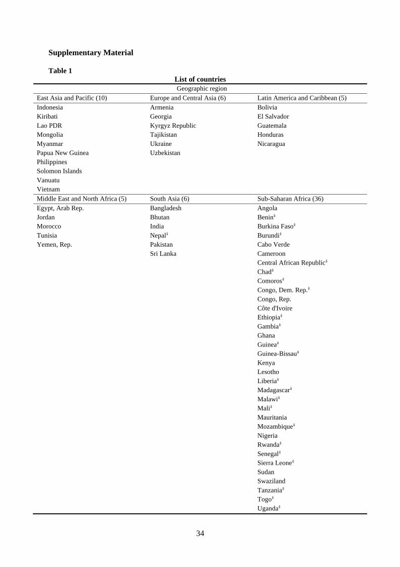
34

Supplementary Material

Table 1

List of countries

Geographic region

East Asia and Pacific (10) Europe and Central Asia (6) Latin America and Caribbean (5)

Indonesia

Kiribati

Lao PDR

Mongolia

Myanmar

Papua New Guinea

Philippines

Solomon Islands

Vanuatu

Vietnam

Armenia

Georgia

Kyrgyz Republic

Tajikistan

Ukraine

Uzbekistan

Bolivia

El Salvador

Guatemala

Honduras

Nicaragua

Middle East and North Africa (5) South Asia (6) Sub-Saharan Africa (36)

Egypt, Arab Rep.

Jordan

Morocco

Tunisia

Yemen, Rep.

Bangladesh

Bhutan

India

Nepal⸙

Pakistan

Sri Lanka

Angola

Benin⸙

Burkina Faso⸙

Burundi⸙

Cabo Verde

Cameroon

Central African Republic⸙

Chad⸙

Comoros⸙

Congo, Dem. Rep.⸙

Congo, Rep.

Côte d'Ivoire

Ethiopia⸙

Gambia⸙

Ghana

Guinea⸙

Guinea-Bissau⸙

Kenya

Lesotho

Liberia⸙

Madagascar⸙

Malawi⸙

Mali⸙

Mauritania

Mozambique⸙

Nigeria

Rwanda⸙

Senegal⸙

Sierra Leone⸙

Sudan

Swaziland

Tanzania⸙

Togo⸙

Uganda⸙

35

Zambia

Zimbabwe⸙

Notes: ⸙ denotes that the respective country belongs to the low income group.

Table 2

Variables definition

Variable Defintion Source

CO2 CO2 emissions totals of fossil fuel use and industrial

processes (ktonnes)

The European Commission, Joint Research Centre

(EC-JRC)/Netherlands Environmental Assessment

Agency (PBL). Emissions Database for Global

Atmospheric Research (EDGAR), release

EDGARv4.3.2_FT2016 (1970 - 2016). Janssens-

Maenhout, G., Crippa, M., Guizzardi, D., Muntean,

M., Schaaf, E., Olivier, J.G.J., Peters, J.A.H.W.,

Schure, K.M., Fossil CO2 and GHG emissions of

all world countries, EUR 28766 EN,Publications

Office of the European Union, Luxembourg, 2017,

ISBN 978-92-79-73207-2, doi:10.2760/709792,

JRC107877

(http://edgar.jrc.ec.europa.eu/overview.php?v=boo

klet2017&dst=CO2emi)

CO2_T CO2 emission from transport

CO2_B CO2 emission from buildings

CO2_OIC CO2 emission from other industrial combustion

CO2_NC CO2 emission from non-combustion

CO2_PI CO2 emission from power industry

GDP GDP based on purchasing power parity (PPP) (constant

2011 international $)

The World Bank, World Bank Indicators

(https://databank.worldbank.org/data/home.aspx)

URB Urban population (% of total population)

RENG Renewable energy consumption (% of total final energy

consumption)

EINT Energy intensity level of primary energy computed as total

primary energy supply over GDP measured in constant

2011 US dollars at PPP (MJ/$2011 PPP GDP)

POP Total midyear population

AGRI Agriculture, value added (% of GDP)

IND Industry, value added (% of GDP)

SERV Services, value added (% of GDP)

TRADE Trade (% of GDP)

FRENTS Forest rents (% of GDP)

CREDIT Domestic credit to private sector (% of GDP)

GDPc GDP per capita based on purchasing power parity (PPP)

(constant 2011 international $)

REM Migrant remittance inflows (nominal US$ million) The World Bank staff calculation based on data

from IMF Balance of Payments Statistics database

and data releases from central banks, national

statistical agencies, and World Bank country desks

(https://www.worldbank.org/en/topic/labormarkets

/brief/migration-and-remittances)

CO2c CO2 per capita emissions totals of fossil fuel use and

industrial processes (ktonnes)

Authors’ computation based on The European

Commission, Joint Research Centre (EC-

JRC)/Netherlands Environmental Assessment

Agency (PBL) (CO2 emissions:

http://edgar.jrc.ec.europa.eu/overview.php?v=book

let2017&dst=CO2emi) and World Bank Indicators

data (population:

https://databank.worldbank.org/data/home.aspx)

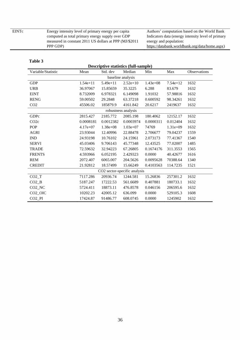
36

EINTc Energy intensity level of primary energy per capita

computed as total primary energy supply over GDP

measured in constant 2011 US dollars at PPP (MJ/$2011

PPP GDP)

Authors’ computation based on the World Bank

Indicators data (energy intensity level of primary

energy and population:

https://databank.worldbank.org/data/home.aspx)

Table 3

Descriptive statistics (full-sample)

Variable/Statistic Mean Std. dev Median Min Max Observations

baseline analysis

GDP 1.54e+11 5.49e+11 2.52e+10 1.43e+08 7.54e+12 1632

URB 36.97067 15.85659 35.3225 6.288 83.679 1632

EINT 8.732009 6.978321 6.149098 1.91032 57.98816 1632

RENG 59.00502 29.2848 63.37218 0.600592 98.34261 1632

CO2 45506.02 185879.9 4161.842 20.6217 2419637 1632

robustness analysis

GDPc 2815.427 2185.772 2085.198 180.4062 12152.17 1632

CO2c 0.0008181 0.0012382 0.0003974 0.0000311 0.012404 1632

POP 4.17e+07 1.38e+08 1.03e+07 74769 1.31e+09 1632

AGRI 23.93044 12.40996 22.88478 2.706677 79.04237 1559

IND 24.93198 10.76102 24.15961 2.073173 77.41367 1540

SERVI 45.03406 9.706143 45.77348 12.43525 77.02007 1485

TRADE 72.59632 32.94223 67.26805 0.1674176 311.3553 1565

FRENTS 4.593966 6.052195 2.429323 0.0000 40.42677 1616

REM 2072.407 6065.007 204.5626 0.0095628 70388.64 1340

CREDIT 21.92812 18.57499 15.66249 0.4103563 114.7235 1521

CO2 sector-specific analysis

CO2_T 7117.286 20936.74 1244.581 15.26836 257301.2 1632

CO2_B 5187.247 17222.53 561.6689 0.407881 180733.1 1632

CO2_NC 5724.411 18873.11 476.8578 0.046156 206595.6 1632

CO2_OIC 10202.23 42005.12 636.099 0.0000 529105.3 1608

CO2_PI 17424.87 91486.77 608.0745 0.0000 1245902 1632

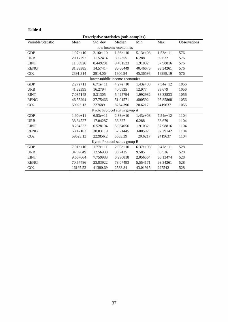
37

Table 4

Descriptive statistics (sub-samples)

Variable/Statistic Mean Std. dev Median Min Max Observations

low income economies

GDP 1.97e+10 2.16e+10 1.36e+10 5.13e+08 1.53e+11 576

URB 29.17297 11.52414 30.2355 6.288 59.632 576

EINT 11.83926 8.449231 9.401523 1.91032 57.98816 576

RENG 81.83385 14.57414 86.66449 40.46676 98.34261 576

CO2 2391.314 2914.064 1306.94 45.36593 18988.19 576

lower-middle income economies

GDP 2.27e+11 6.71e+11 4.27e+10 1.43e+08 7.54e+12 1056

URB 41.22395 16.2794 40.0925 12.977 83.679 1056

EINT 7.037145 5.31305 5.425794 1.992982 38.33533 1056

RENG 46.55294 27.75466 51.01571 .600592 95.85808 1056

CO2 69023.13 227689 8254.396 20.6217 2419637 1056

Kyoto Protocol status group A

GDP 1.90e+11 6.53e+11 2.88e+10 1.43e+08 7.54e+12 1104

URB 38.34527 17.04287 36.327 6.288 83.679 1104

EINT 8.284522 6.528194 5.964056 1.91032 57.98816 1104

RENG 53.47162 30.03119 57.21445 .600592 97.29142 1104

CO2 59523.13 222856.2 5533.39 20.6217 2419637 1104

Kyoto Protocol status group B

GDP 7.91e+10 1.77e+11 2.00e+10 6.37e+08 9.47e+11 528

URB 34.09649 12.56938 33.7425 9.585 65.526 528

EINT 9.667664 7.759983 6.990818 2.056564 50.13474 528

RENG 70.57486 23.83922 78.07493 5.554171 98.34261 528

CO2 16197.52 41380.69 2583.84 43.01915 227542 528

38

Table 5

Panel SVAR-Granger causality Wald test

[Equation] \ Excluded variable chi2 df prob > chi2

[GDP]

URB 1.083 1 (0.298)

EINT 1.531 1 (0.216)

RENG 2.812* 1 (0.094)

CO2 0.469 1 (0.493)

ALL 5.921 4 (0.205)

[URB]

GDP 10.608*** 1 (0.001)

EINT 0.167 1 (0.683)

RENG 2.247 1 (0.134)

CO2 1.989 1 (0.158)

ALL 16.152*** 4 (0.003)

[EINT]

GDP 22.044*** 1 (0.000)

URB 0.149 1 (0.699)

RENG 0.563 1 (0.453)

CO2 0.805 1 (0.370)

ALL 23.092*** 4 (0.000)

[RENG]

GDP 11.287*** 1 (0.001)

URB 5.934** 1 (0.015)

EINT 2.131 1 (0.144)

CO2 1.273 1 (0.259)

ALL 23.727*** 4 (0.000)

[CO2]

GDP 4.828** 1 (0.028)

URB 15.787*** 1 (0.000)

EINT 6.179** 1 (0.013)

RENG 1.313 1 (0.252)

ALL 22.787*** 4 (0.000)

Notes: H0 is ''Excluded variable does not Granger-cause equation variable'', while according

to H1 ''Excluded variable Granger-causes equation variable. ***, **, *, denotes significance at

the 1%, 5% and 10% level, respectively.

39

Table 6

Panel SVAR selection order criteria

Lag CD J J p-value MBIC MAIC MQIC

1 0.988 70.449 0.019 -270.824 -25.550 -117.853

2 0.988 48.099 0.033 -179.417 -15.900 -77.435

3 0.988 17.601 0.345 -96.156 -14.398 -45.166

Observations 1224

Panels 68

Notes: Model and moment selection criteria are computed using the first four lags of variables.

Table 7

Model stability condition

Eigenvalue

Real Imaginary Modulus

0.940 0 0.940

0.372 0 0.372

-0.081 0 0.081

-0.045 0 0.045

0.022 0 0.022

Notes: All the eigenvalues lie inside the unit circle. The GMM panel

SVAR model satisfies stability condition.

Figure 1

Inverted roots of AR characteristics polynomial (GMM-SVAR)

40

Table 8

First-order panel SVAR-GMM estimates

Response to

Response of GDPt-1 URBt-1 EINTt-1 RENGt-1 CO2t-1

GDP 0.3746*** -0.2343 0.0190 -0.0292* 0.0083

(0.0436) (0.2251) (0.0154) (0.0174) (0.0122)

URB 0.0066*** 0.9398*** 0.0002 0.0010 0.0011

(0.0020) (0.0241) (0.0007) (0.0007) (0.0007)

EINT -0.2868*** 0.1219 -0.0517 0.0271 0.0246

(0.0610) (0.3158) (0.0427) (0.0362) (0.0274)

RENG -0.1375*** 0.4409** -0.0481 -0.0618 -0.0263

(0.0409) (0.1810) (0.0329) (0.0497) (0.0233)

CO2 0.1628** 1.9181*** 0.1078** 0.0536 0.0072

(0.0741) (0.4827) (0.0433) (0.0468) (0.0367)

Observations 1428

Countries 68

Notes: The five-variable one lag panel SVAR is estimated by GMM, using first four lags of the variables as

instruments. The country-specific fixed effects are removed during estimation via the Helmert transformation.

Reported numbers display the coefficients of regressing the row variables on first lag of the column variables.

Standard errors robust to heteroskedasticity and serial correlation in brackets. ***, **, *, denotes significance at

the 1%, 5% and 10% level, respectively.

41

Figure 2

Orthogonalized IRFs

Observations: 1428 • Groups: 68

Notes: The continuous line denotes the impulse response functions. The dashed lines stand for the associated

95% confidence interval computed based on 1000 Monte Carlo simulations.

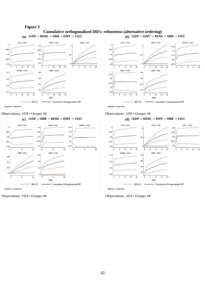
42

Figure 3

Cumulative orthogonalized IRFs: robustenss (alternative ordering)

(a) (b)

Observations: 1428 • Groups: 68 Observations: 1428 • Groups: 68

(c) (d)

Observations: 1428 • Groups: 68 Observations: 1428 • Groups: 68

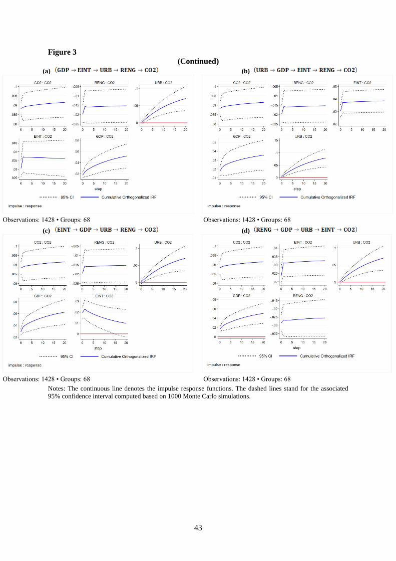
43

Figure 3

(Continued)

(a) (b)

Observations: 1428 • Groups: 68 Observations: 1428 • Groups: 68

(c) (d)

Observations: 1428 • Groups: 68 Observations: 1428 • Groups: 68

Notes: The continuous line denotes the impulse response functions. The dashed lines stand for the associated

95% confidence interval computed based on 1000 Monte Carlo simulations.

44

Figure 4

Cumulative orthogonalized IRFs: altering the sample & variables in per capita terms

(a) period: 1992-2008 (b) period: 1992-2010

Observations: 1020 • Groups: 68 Observations: 1156 • Groups: 68

(c) period: 1996-2015 (d) without: Egypt, Jordan, Mauritania, Morocco, Sudan, Tunisia,

Yemen

Observations: 1292 • Groups: 68 Observations: 1281 • Groups: 61

45

Figure 4

(Continued)

(e) without: Angola, Congo Rep., Egypt, Indonesia, Nigeria,

Vietnam

(f) GDP and CO2 in per capita terms

Observations: 1302 • Groups: 62 Observations: 1428 • Groups: 68

(g) GDP, EINT, and CO2 in per capita terms

Observations: 1428 • Groups: 68

Notes: The continuous line denotes the impulse response functions. The dashed lines stand for the associated

95% confidence interval computed based on 1000 Monte Carlo simulations.

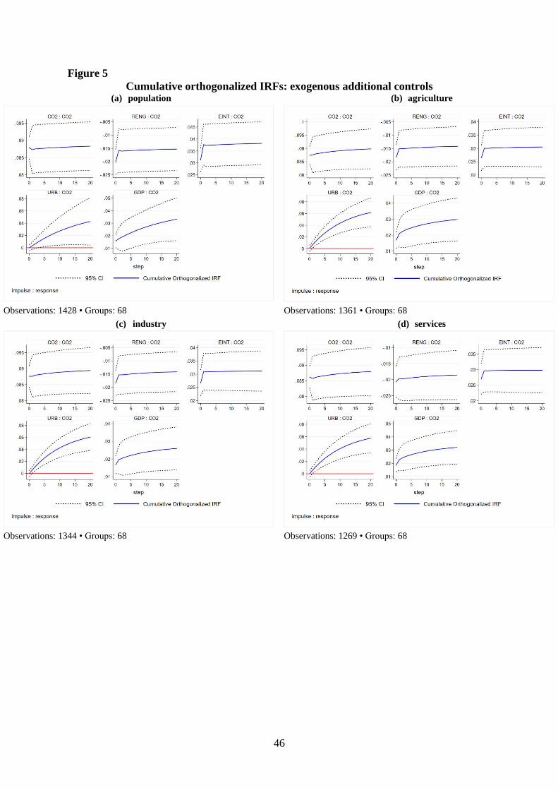
46

Figure 5

Cumulative orthogonalized IRFs: exogenous additional controls (a) population (b) agriculture

Observations: 1428 • Groups: 68 Observations: 1361 • Groups: 68

(c) industry (d) services

Observations: 1344 • Groups: 68 Observations: 1269 • Groups: 68

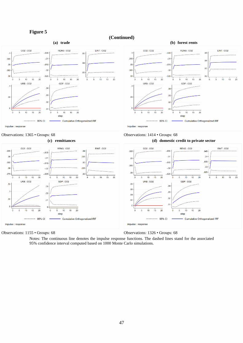
47

Figure 5

(Continued) (a) trade (b) forest rents

Observations: 1365 • Groups: 68 Observations: 1414 • Groups: 68

(c) remittances (d) domestic credit to private sector

Observations: 1155 • Groups: 68 Observations: 1326 • Groups: 68

Notes: The continuous line denotes the impulse response functions. The dashed lines stand for the associated

95% confidence interval computed based on 1000 Monte Carlo simulations.

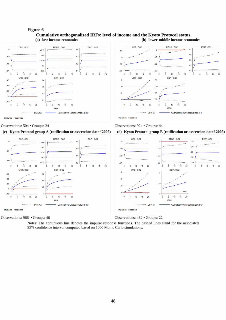
48

Figure 6

Cumulative orthogonalized IRFs: level of income and the Kyoto Protocol status (a) low income economies (b) lower-middle income economies

Observations: 504 • Groups: 24 Observations: 924 • Groups: 44

(c) Kyoto Protocol group A (ratification or asscension date 2005) (d) Kyoto Protocol group B (ratification or asscension date 2005)

Observations: 966 • Groups: 46 Observations: 462 • Groups: 22

Notes: The continuous line denotes the impulse response functions. The dashed lines stand for the associated

95% confidence interval computed based on 1000 Monte Carlo simulations.

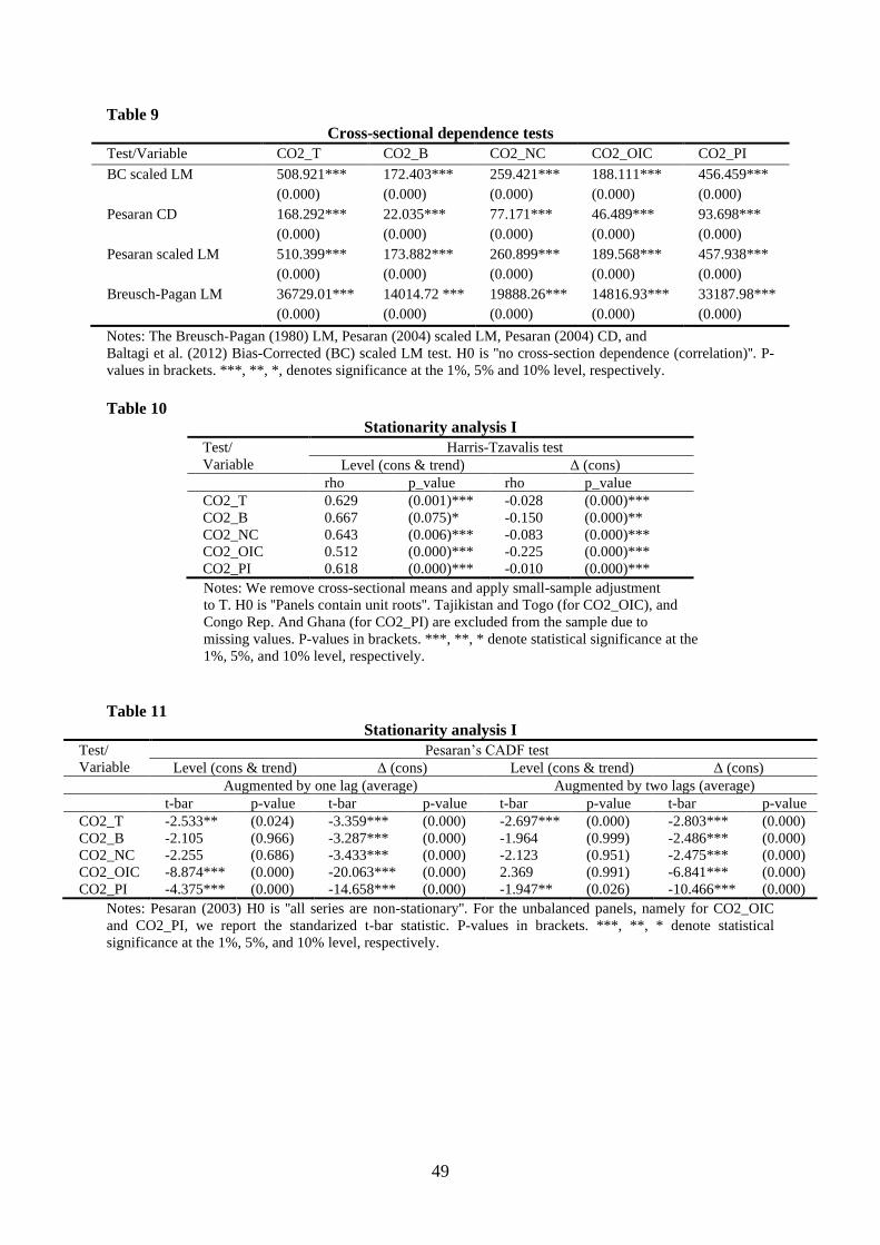
49

Table 9

Cross-sectional dependence tests

Test/Variable CO2_T CO2_B CO2_NC CO2_OIC CO2_PI

BC scaled LM 508.921*** 172.403*** 259.421*** 188.111*** 456.459***

(0.000) (0.000) (0.000) (0.000) (0.000)

Pesaran CD 168.292*** 22.035*** 77.171*** 46.489*** 93.698***

(0.000) (0.000) (0.000) (0.000) (0.000)

Pesaran scaled LM 510.399*** 173.882*** 260.899*** 189.568*** 457.938***

(0.000) (0.000) (0.000) (0.000) (0.000)

Breusch-Pagan LM 36729.01*** 14014.72 *** 19888.26*** 14816.93*** 33187.98***

(0.000) (0.000) (0.000) (0.000) (0.000)

Notes: The Breusch-Pagan (1980) LM, Pesaran (2004) scaled LM, Pesaran (2004) CD, and

Baltagi et al. (2012) Bias-Corrected (BC) scaled LM test. H0 is ''no cross-section dependence (correlation)''. P-

values in brackets. ***, **, *, denotes significance at the 1%, 5% and 10% level, respectively.

Table 10

Stationarity analysis I

Test/

Variable

Harris-Tzavalis test

Level (cons & trend) Δ (cons)

rho p_value rho p_value

CO2_T 0.629 (0.001)*** -0.028 (0.000)***

CO2_B 0.667 (0.075)* -0.150 (0.000)**

CO2_NC 0.643 (0.006)*** -0.083 (0.000)***

CO2_OIC 0.512 (0.000)*** -0.225 (0.000)***

CO2_PI 0.618 (0.000)*** -0.010 (0.000)***

Notes: We remove cross-sectional means and apply small-sample adjustment

to T. H0 is ''Panels contain unit roots''. Tajikistan and Togo (for CO2_OIC), and

Congo Rep. And Ghana (for CO2_PI) are excluded from the sample due to

missing values. P-values in brackets. ***, **, * denote statistical significance at the

1%, 5%, and 10% level, respectively.

Table 11

Stationarity analysis I

Test/

Variable

Pesaran’s CADF test

Level (cons & trend) Δ (cons) Level (cons & trend) Δ (cons)

Augmented by one lag (average) Augmented by two lags (average)

t-bar p-value t-bar p-value t-bar p-value t-bar p-value

CO2_T -2.533** (0.024) -3.359*** (0.000) -2.697*** (0.000) -2.803*** (0.000)

CO2_B -2.105 (0.966) -3.287*** (0.000) -1.964 (0.999) -2.486*** (0.000)

CO2_NC -2.255 (0.686) -3.433*** (0.000) -2.123 (0.951) -2.475*** (0.000)

CO2_OIC -8.874*** (0.000) -20.063*** (0.000) 2.369 (0.991) -6.841*** (0.000)

CO2_PI -4.375*** (0.000) -14.658*** (0.000) -1.947** (0.026) -10.466*** (0.000)

Notes: Pesaran (2003) H0 is ''all series are non-stationary''. For the unbalanced panels, namely for CO2_OIC

and CO2_PI, we report the standarized t-bar statistic. P-values in brackets. ***, **, * denote statistical

significance at the 1%, 5%, and 10% level, respectively.

50

Additional References for the Supplementary Material

Janssens-Maenhout, G., Crippa, M., Guizzardi, D., Muntean, M., Schaaf, E., Olivier,

J.G.J., Peters, J.A.H.W. and Schure, K.M., 2017. Fossil CO2 and GHG emissions of

all world countries. EUR 28766 EN, Publications Office of the European Union,

Luxembourg, ISBN 978-92-79-73207-2, doi:10.2760/709792, JRC107877.