Developing Analytical Framework to Measure Robustness of Peer-to-Peer Networks

Niloy Ganguly

Client/Server Architecture

Well known, powerful, reliable server is a data source

Clients request data from server

Very successful model WWW (HTTP), FTP, Web services, etc.

Server

Client

Client Client

Client

Internet

Client/Server Limitations

Scalability is hard to achieve (load balancing)

Presents a single point of failure (fault tolerance)

Network bandwidth adds the bottleneck problem

Requires administration

P2P systems try to address these limitations

Peer to Peer Networks

All nodes are both clients and servers i.e. Servent (SERVer+cliENT)

Provide and consume data Any node can initiate a connection

No centralized data source

“The ultimate form of democracy on the Internet”

Node

Node

Node Node

Node

Internet

Peer to Peer Networks Popular medium for file sharing and other

applications like IP telephony, distributed storage, publisher subscriber system,etc.

Overlay Networks Logical network above the physical p2p network Importance of the topology of overlay networks

Spread of information in the network Stability of the network due to dynamic nature of

the peers.

Overlay Network

• An overlay network is built on top of physical network. Nodes in the overlay can be thought of as being connected by virtual or logical links, each of which corresponds to a path, perhaps through many physical links, in the underlying network.

Examples:

• P2P overlay network run on top of the Internet.

Overlay Network

• An overlay network is built on top of physical network. Nodes in the overlay can be thought of as being connected by virtual or logical links, each of which corresponds to a path, perhaps through many physical links, in the underlying network.

Examples:

• P2P overlay network run on top of the Internet.

Overlay edge

Overlay Network

• An overlay network is built on top of physical network. Nodes in the overlay can be thought of as being connected by virtual or logical links, each of which corresponds to a path, perhaps through many physical links, in the underlying network.

Examples:

• P2P overlay network run on top of the Internet.

Overlay edge

Motivation Peers in the p2p system join and leave

network randomly without any central coordination.

Makes overlay structures highly dynamic in nature. Frequently it partitions the network into smaller

fragments Communication between peers become impossible.

In this work, our primary goal is to develop an analytical framework to examine the stability of the various overlay structures against dynamic movement of peers.

Overview Various Overlay Structures –

Topology Dynamic movements of peers Stability criterion Analytical framework

Topology of the Overlay Networks Topology of the overlay networks can be modeled

From experimentally collected data of overlay topology By various random graphs characterized by degree distribution

Examples: E-R graph

N number of vertices are connected with probability p. Probability of any randomly chosen node having degree k becomes

Degree distribution follows Poisson distribution. Maintains homogeneous connectivity

Scale free network Inhomogeneous connectivity Majority of nodes have only a few links and very few highly connected

nodes control the connectivity of entire network. Degree distribution follows power law distribution

!k

ezp

zk

k

ckpk

Topology of the Overlay networks

Superpeer networks Small fraction of nodes are superpeers and rest are

peers Each superpeer node is connected with a set of peers Superpeers are connected among themselves KaZaA adopted this kind of topology Follows Bimodal degree distribution Mathematically if otherwise

Superpeer Node

Peer node

0kp ml kkk ,0kp

Percolation and Peer Movement Movement of the peers can be modeled by

various kinds of node failures in the random graph

Degree independent node failure Probability of removal of a node is constant &

degree independent Targeted Attack

Nodes having highest connectivity is removed first Degree dependent node failure

Probability of removal of a node is inversely proportional to the degree of that node

Peers having lower connectivity are less stable because they enter and leave network frequently.

Stability Metric - Percolation Threshold Percolation threshold is the critical fraction of nodes

whose removal disintegrates the giant component into smaller fragmented components

We use percolation threshold as the stability metric for our analysis.

Initially all the nodes in the network are connected.

Forms a single giant component.

Percolation Threshold

Initial single connected component

f fraction of nodes

removed

Giant component still

exists

Percolation Threshold

Initial single connected component

f fraction of nodes

removed

Giant component still

exists

fc fraction of nodes

removed

The entire graph breaks into

smaller

fragments Therefore fc becomes percolation threshold

Stability Analysis We use generating function formalism

to perform stability analysis. According to this formalism, general

formula for the stability of the giant component with respect to any type of graph (pk) and any kind of failure (qk) becomes

0

0)1(k

kkk qkqkp

Generating function formalism Generating function:

Formal power series whose coefficients encode information.

Here encode information about a sequence

Used to understand different properties of the graph generates the probability

distribution of the vertex degrees. Average degree

0

0 )(k

kk xpxG

)1('0Gkz

.........)( 33

2210 xaxaxaaxP

,.....),,( 210 aaa

Stability Analysis and specifies the network

topology and failure models respectively.

specifies the probability of a node having degree to be present in the network after the process of removal of some portion of nodes is completed.

becomes the corresponding generating function.

kp kq

kk qp .k

0

0 )(k

kkk xqpxF

Stability Analysis

Topology specified by kp

Fraction of nodes removed according to )1( kq

kk qp .

specifies the probability of a node having degree k after the process of node removal

Stability Analysis Let F1(x) generates the distribution of outgoing edges of the

first neighbor of a randomly chosen node. F1(x)=F’0(x)/z

H1(x) generates the distribution of the component sizes reached by following a random edge.

H1(x) satisfies a self-consistency condition of the form H1(x)=1-F1(1)+xF1(H1(x))

Randomly selected node ‘A’

A

Degree distribution of the first neighbor of ‘A’

Stability Analysis

Distribution for the component size to which a randomly selected node belongs to generated by H0(x) where

H0(x)=1-F0(1)+xF0(H1(x))

= + + + + …….

Schematic representation of the sum rule for the connected component of vertices reached by following a random edge. (Self consistency condition)

Stability Analysis Average size of the component

Which diverges when F1’(1)=1

This equation states the critical condition for the stability of giant component

For any kind of graph ( pk) Undergoing any kind of failure (1-qk)

0

0)1(k

kkk qkqkp

)1('1

)1()1(')1()1('

1

1000 F

FFFsH

Stability at various scenario

Stability of generalized random graphs undergoing various failures

Degree Independent random failure : In this case qk=q=qc

Using

Therefore percolation threshold

1

12

kk

qc

1

11 2

kk

fc

0

0)1(k

kkk qkqkp

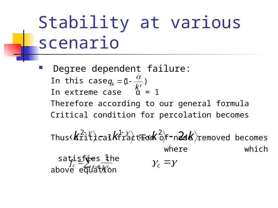
Stability at various scenario Degree dependent failure:

In this caseIn extreme case α = 1Therefore according to our general formula Critical condition for percolation becomes

Thus critical fraction of node removed becomes where which satisfies theabove equation

)1(

k

qk

kkkk 2212

0

1kc ck

f c

Case Study:Superpeer Networks Recently superpeer networks have been

adopted by many p2p systems like KaZaA.

A small fraction of nodes are superpeers and rest are peers.

Connectivity of superpeers are much more higher than the peers.

It can be modeled by bimodal degree distribution.

Case Study:Superpeer Networks Degree independent failure:

According to our framework, critical fraction for superpeer networks

where r = fraction of peers Superpeer degree Average degree of the network

222 221

mmmmc rkkkrkrkkkk

rkf

mkk

Case Study:Superpeer networksDegree independent failure

0 0.2 0.4 0.6 0.8 10

0.2

0.4

0.6

0.8

1

r (fraction of peers)

f c (cr

itica

l fra

ctio

n)

Km=25

Km=30

Km=40

Comparative study between theoretical and experimental

results

Theoretical Experimental

0 0.2 0.4 0.6 0.8 10.8

0.85

0.9

0.95

1

r (fraction of peers)

f c (cr

itica

l fra

ctio

n)

Km=25

Km=30

Km=40

Observations Increase of the fraction of superpeers (specially

above 15% to 20%) increases stability of the network.

Experimental result indicates the optimum superpeer to peer ratio for which overlay networks becomes most stable for this kind of failure.

Due to the contradiction of theoretical and practical concept of giant component, there is a little difference between theoretical and experimental results.

Case Study:Superpeer Networks Degree dependent failure: In this case, the value of which

percolates the network can be derived from our general formula and becomes

where Superpeer degree Average degree of the network

c

m

mm

c kk

kkkk

ln1

2)1(ln

1

mkk

Case Study:Superpeer networksDegree dependent failure Comparative study between theoretical and experimental

results

Theoretical Experimental

10 15 20 25 300.01

0.02

0.03

0.04

0.05

0.06

0.07

Km (Degree of superpeers)

c

<k>=8 <k>=12 <k>=16 Line fitting curve

10 15 20 25 300

0.02

0.04

0.06

0.08

0.1

Km (Degree of superpeers)

c

<k>=8 <k>=12 <k>=16 Line fitting curve

Observations

With the increase of superpeer degree, the value of γc that percolates the network decreases.

Thus it improves the stability of the network and the improvement follows hyperbolic trajectories.

Result supports our intuitive notion of giant component.

Conclusion Contribution of our work

Development of general framework to analyze the stability of p2p overlay networks.

Modeling the behavior of the peers using degree independent as well as degree dependent node failure.

Case Study : stability analysis of the superpeer networks.

Perform a comparative study between theoretical and experimental results to show the effectiveness of our theoretical model.

Future Work We have to perform a detailed comparative study of

stability of various overlay structures. Example: E-R networks,scale free networks, various kinds

of superpeer networks like Mixed Poisson and bimodal structures.

Peer movements can be modeled by various kinds of node failures and attacks where nodes having more importance are been targeted.

Importance of a node is determined by degree centrality, betweenness centrality, eigenvector centrality etc

Finally a comparative stability analysis of all these topologies with respect to combination of different attacks and failures.

Stability Criterion Giant Component

Most of the nodes in the network are connected to form a large connected component

After removing a fraction of nodes from the network A large fraction of nodes still remains connected. Although average distance increases.

A fraction of nodes removed from the

network

Percolation process Giant

component

Percolation Process:Degree independent failure

Occupied Node

Unoccupied Node

Nodes to be removed are selected at random (do not dependent on their

degree)

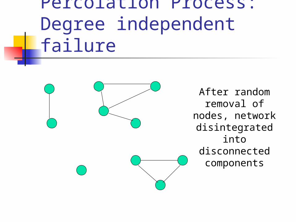
Percolation Process: Degree independent failure

After random removal of nodes,

network disintegrated into

disconnected components

Percolation Process: Targeted Attack

Highly connected nodes

Occupied Node

Unoccupied Node

Highly connected nodes are attacked first

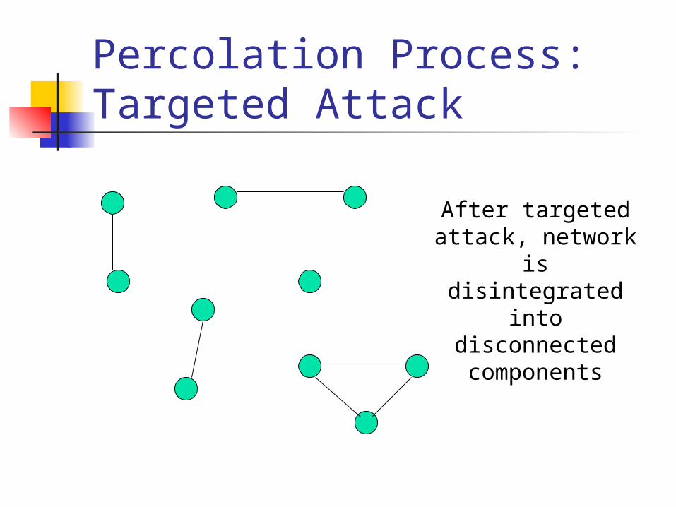
Percolation Process: Targeted Attack

After targeted attack, network is disintegrated into

disconnected components

Percolation Process: Degree dependent failure

Occupied Node

Unoccupied Node

Nodes to be removed are inversely proportional to its degree

Percolation Process: Degree dependent failure

After degree dependent

failure , network is disintegrated into

spited components

Movement of peers Topology of the overlay networks can be

modeled by various real world networks. Movement of peers can be represented by

percolation processes in those graphs. We study the stability of various

topologies by measuring the effect of percolation on the connectivity of the graph.