Embed Size (px)
Citation preview

UPTEC STS15 008
Examensarbete 30 hpJune 2015
Developing a Recommender Systemfor a Mobile E-commerce Application
Adam Elvander

Teknisk- naturvetenskaplig fakultet UTH-enheten Besöksadress: Ångströmlaboratoriet Lägerhyddsvägen 1 Hus 4, Plan 0 Postadress: Box 536 751 21 Uppsala Telefon: 018 – 471 30 03 Telefax: 018 – 471 30 00 Hemsida: http://www.teknat.uu.se/student
Abstract
Developing a Recommender System for a MobileE-commerce Application
Adam Elvander
This thesis describes the process of conceptualizing and developing a recommendersystem for a peer-to-peer commerce application. The application in question is calledPlick and is a vintage clothes marketplace where private persons and smaller vintageretailers buy and sell secondhand clothes from each other. Recommender systems is arelatively young field of research but has become more popular in recent years withthe advent of big data applications such as Netflix and Amazon. Examples ofrecommender systems being used in e-marketplace applications are however stillsparse and the main contribution of this thesis is insight into this sub-problem inrecommender system research. The three main families of recommender algorithmsare analyzed and two of them are deemed unfitting for the e-marketplace scenario.Out of the third family, collaborative filtering, three algorithms are described,implemented and tested on a large subset of data collected in Plick that consistsmainly of clicks made by users on items in the system. By using both traditional andnovel evaluation techniques it is further shown that a user-based collaborative filteringalgorithm yields the most accurate recommendations when compared to actual userbehavior. This represents a divergence from recommender systems commonly usedin e-commerce applications. The paper concludes with a discussion on the cause andsignificance of this difference and the impact of certain data-preprocessing techniqueson the results.
ISSN: 1650-8319, UPTEC STS15 008Examinator: Elísabet AndrésdóttirÄmnesgranskare: Michael AshcroftHandledare: Jimmy Heibert

1 Introduction ___________________________________________________________________ 2
1.1 Overview ________________________________________________________________ 2
1.2 Project Outline ____________________________________________________________ 2
1.3 Questions ________________________________________________________________ 3
1.4 Methods and Tools _________________________________________________________ 3
1.5 Report Structure ___________________________________________________________ 3
2 Recommender Systems _________________________________________________________ 4
2.1 About Data _______________________________________________________________ 4 2.1.1 What is a Rating? ____________________________________________________ 4 2.1.2 On Explicit and Implicit Ratings _________________________________________ 5
2.2 Families of Recommender Algorithms __________________________________________ 6 2.2.1 Content-based Filtering _______________________________________________ 6 2.2.2 Knowledge-based Filtering ____________________________________________ 7 2.2.3 Collaborative Filtering ________________________________________________ 8
2.2.3.1 User-based __________________________________________________ 8 2.2.3.2 Item-based __________________________________________________ 9 2.2.3.3 Matrix Factorization __________________________________________ 10
2.3 Recommendation Engines __________________________________________________ 10 2.3.1 Data Preprocessing _________________________________________________ 11 2.3.2 Similarity Measures _________________________________________________ 11 2.3.3 Predicting and Recommending ________________________________________ 12
3 System Information ___________________________________________________________ 13
3.1 Data in the E-Marketplace __________________________________________________ 13
3.2 The Plick Case ___________________________________________________________ 13 3.2.1 System Architecture _________________________________________________ 14 3.2.2 Features __________________________________________________________ 16 3.2.3 Users and Items ____________________________________________________ 16 3.2.4 Data _____________________________________________________________ 16
4 Selecting a Recommender System _______________________________________________ 17
4.1 Matching Data and Algorithms _______________________________________________ 17 4.1.1 Content-based methods _____________________________________________ 17 4.1.2 Knowledge-based methods ___________________________________________ 18 4.1.3 Collaborative Filtering methods ________________________________________ 18
4.1.3.1 User-based _________________________________________________ 19 4.1.3.2 Item-based _________________________________________________ 20 4.1.3.3 Matrix Factorization __________________________________________ 20
4.2 Implementation and Evaluation of Candidate Algorithms __________________________ 21 4.2.1 Data Selection and Preprocessing _____________________________________ 22 4.2.2 Item-Based ________________________________________________________ 23 4.2.3 Matrix Factorization _________________________________________________ 25 4.2.4 User-Based _______________________________________________________ 26
4.3 Extensions and Improvements _______________________________________________ 28 4.3.1 Rating Aggregation _________________________________________________ 28 4.3.2 Rating Normalization ________________________________________________ 29 4.3.4 Significance Weighting_______________________________________________ 30

1
4.4 Choosing an Algorithm: Evaluating Recommendations ____________________________ 31
5 Final System _________________________________________________________________ 33
5.1 Parameter Tuning _________________________________________________________ 33 5.1.1 Algorithm Parameters _______________________________________________ 33 5.1.2 Rating Aggregation Weights __________________________________________ 38
5.2 Schemas _______________________________________________________________ 39 5.2.1 Algorithm _________________________________________________________ 39 5.2.2 System ___________________________________________________________ 40
6 Discussion and Conclusions ___________________________________________________ 40
7 References __________________________________________________________________ 43

2
1 Introduction
1.1 Overview
The goal of this project is a functional recommendation algorithm integrated into the mobile
application Plick. Plick is an e-marketplace application for vintage clothing with a user-base in
the thousands. The application was launched in 2013 and has seen an increasing stream of
articles of clothing being posted, leading to a huge selection of ads for potential buyers to wade
through. This problem of an overwhelming supply is closely related to the more general expanse
of available information made possible by the internet, by many researchers referred to as
information overload.1 It is exactly this issue that recommender systems are designed to address
and is why Plick was considered in need of some form of personalized filtration of the available
inventory.
The market for vintage clothes has benefited greatly from the advent of e-commerce, bringing
buyers and sellers together with minimal effort. It has been further boosted by an increased
interest in environmentally friendly consumption habits in the past few decades. It is in this
emerging market that Plick exists, making use of the technologically driven simplicity of
connecting consumers with both individual sellers but also larger retailers of used clothes
without their own online platforms.
In the recommender systems research field the e-marketplace is a new and very atypical case
that brings unique challenges to the fore and that may require novel approaches to tackle.2 An
example of these challenges is the fact that in the selling of used clothes there is usually only one
of each item in the inventory and when that is sold it is gone from the system. This makes it
impossible to use a recommendation approach like Amazon’s “people who bought this also
bought…” There are many issues like this that come with the peer-to-peer structure of an
application like Plick. These issues are the reason Plick is such an interesting case to apply
recommender systems technology on. Meaningful relationships in the data have to be identified
in a changeable, almost volatile, environment.
The project was carried out in the Uppsala offices of Swace Digital, Plick’s parent company.
1.2 Project Outline
The outline and details of the project were decided on by the master’s student in collaboration
with the creators and developers of Plick. The project was carried out in three overarching
stages:
1. Exhaustive study of the research field and the commonly used techniques. From this
baseline a few promising methods were chosen for implementation and evaluation.
2. Implementation and comparison of the selected methods. In this stage the top performing
algorithm was selected for implementation in the live system.
3. Evaluation of the implemented solution and reporting.
1 Francesco Ricci, Lior Rokach, Bracha Shapira, Introduction to Recommender Systems Handbook, Springer, 2011, pp. 2 2 Note the distinction between e-marketplace and e-commerce. E-commerce is the umbrella term for all systems engaged in buying or selling goods and services online whereas an e-marketplace is a system where transactions are peer-to-peer oriented and the goods and services are unique or at least not produced by the owner of the marketplace.

3
1.3 Questions
As the project is a very practical one the questions that can be answered by it are more specific
and technical rather than general and scientific as is often the case with more theoretical projects.
- What are the unique challenges posed by an e-marketplace context when designing a
recommender system? How could they be handled?
- What would a recommender system appropriate for implementation in Plick look
like?
The first question will be a recurring topic throughout the report and will be answered in the last
section. The second question is answered in the form of the system described in section 5 of the
report and is further broached in the final discussion. Note that the second question is not asking
for the best possible system, only an appropriate one.
1.4 Methods and Tools
As stated above, a project of this type is in its nature very practical. The objective is to deliver a
component to a system that will hopefully increase user-activity and sales. However, designing a
reasonably high performing recommender system requires knowledge of the existing methods
and sufficient understanding of the mathematics they employ to apply them to the case in
question. With this in mind the main methodology of this project is to make use of existing
recommender system theory and descriptions of practical recommender applications to tailor a
system that fits the Plick case.
The tools used to carry out this project came mainly in the form of database management
tools and software development tools. To access, track, view and manipulate the data the
following technologies were used: MongoDB, MongoHQ, PostgreSQL, PGAdmin3 and
Microsoft Excel. The MongoDB-programs were used to extract and insert the new data attributes
introduced in this project into the system. The Postgres-programs were used to extract and
analyze the existing historical data. To design the system itself these software development
technologies were used: Python and IDLE (Python GUI) with the Python libraries Cython,
Numpy, PyMongo, Psycopg2 and Pandas. The app-hosting service Heroku and the version
control-system Git were used to deploy the finished system. The literature study was carried out
using Uppsala University’s library resources and Google Scholar.
1.5 Report Structure
The report is divided into seven sections. Section 1 introduces the project and describes the goal
and the questions the project will address. Section 2 gives a background to the research field the
project belongs to. This is followed by section 3 which is a brief overview of the system in
question, Plick. Section 4 describes the process of selecting the methods to be implemented for
testing, based on what was learned in the previous sections. Section 5 describes the fine-tuning
of the final system. Finally, section 6 contains a discussion and the concluding remarks about the
project. Section 7 holds the reference list.

4
1.6 Source Criticism
The main source used in the literature study is the Recommender Systems Handbook. This work
is an edited collection of 24 papers and reports, each with its own author or set of authors. By
including such a vast pool of co-authors it seems the editors of the handbook have attempted to
create a one-stop beginner’s guide to developing recommender systems and it has to some degree
been used as such in this project. Using one source as a theoretical foundation this extensively is
not without its risks. Accepting the formulation of, and solutions to, the recommender system
problem as proposed in the handbook means that this project begins with an outlook already
“zoomed in” on a certain way of doing things. That is, the search for a suitable recommender
system begins with a clear definition of what a recommender system is and what kinds of
recommender systems are used today. While it would perhaps be more academically rewarding
to start by formulating the recommender problem very broadly and drawing up prototype
systems mathematically, the practical limitations of the project prohibit such an ambitious scope.
2 Recommender Systems In this section the results of the literature study are presented, providing an overview of the
current research field.
2.1 About Data
The success of any system that hopes to predict the behavior of a user hinges on the type, volume
and quality of data available. Availability of some data is usually not a problem in this age of big
data, business intelligence and personalized user experiences. In most systems everything is
stored somewhere, even if there is no immediate plan to use the information. The issue facing
someone designing a recommender system is how to discern what data is usable and what it
actually means. In the case of a movie recommendation system of the type that Netflix uses, the
data that is used is a very straightforward set of 1 to 5 stars-ratings connected to a user that can
be immediately fed to a recommendation algorithm. In other cases it is not as simple to interpret
users’ preferences. Consider an online edition of a newspaper. There is probably a multitude of
data stored for each user-article interaction, everything from time spent reading the article to
possible “likes”, comments or social media-shares made by the user, a lot of which is potentially
useful information. The question is how these data points should be understood when thinking
about the preference of the user. How does 5 minutes of reading compare against leaving a
comment in terms of interest shown? How to handle slow readers, social media buffs and other
outlier-behavior?
2.1.1 What is a Rating?
In order to understand usable data we must first define the concept of ratings. In the context of
recommender systems, ratings are used to describe more than just a point on some arbitrary

5
scale. Every piece of information that implies a user’s opinion of or interest in an item3 can be
understood as a rating, or alternatively as a part of an aggregated rating. When aggregating a set
of data points it is important to make use of some standardized way of weighting and scaling
data with different features. In the case of the newspaper website the problem of aggregating
view-time with possible uses of the like-function would be an example of this. What this would
require is a formula that could scale the continuous value of reading time and translate it to a
score comparable to and combinable with the binary data that for example ‘likes’ provide.
In order to make use of rating data it is often stored in one big matrix called the user-item rating
matrix; Fig 1 is an example of this.4 It consists of one axis with all users in the system and
another with all the items. The elements in the matrix are then the ratings given by each user to
each item. Depending on the available data and if the ratings are aggregated this data structure
can actually be made cubic and contain a third axis consisting of the data types used by the
system. For simplicity’s sake only the matrix version will be considered here.
ITEMS
i1 i2 i3 i4 … in
u1 3 5 0 1 → r1n
u2 1 0 0 2 → r2n
USERS u3 3 3 0 3 → r3n
u4 0 0 1 5 → r4n
… ↓ ↓ ↓ ↓ ↘ -
un rn1 rn2 rn3 rn4 - rnn
Fig 1: A generic user-item rating matrix.
2.1.2 On Explicit and Implicit Ratings
With the broad definition of a rating above it is necessary to state that although many things can
be considered ratings they can differ from each other greatly. One important difference is the one
between explicitly given and implicitly interpreted ratings. The first type is very straightforward,
being the type of rating that is consciously provided by a user for no other reason than to indeed
rate the item in question. Examples of this are the Netflix star-ratings and the up- and down-
votes on the website Reddit.com. Implicit ratings are then every piece of information that says
something about a user’s attitude towards an item but is not provided consciously by the user.
3 The term ‘item’ is used for all objects that recommender systems can be applied to. Anything from a movie to a sweater or a master’s thesis report can be an item. 4 Dietmar Jannach, Markus Zanker, Alexander Felfernig, Gerhard Friedrich, Recommender Systems: An Introduction¸ Cambridge University Press, 2011, pp. 13

6
Examples of this could be product viewing history on Amazon.com, reading times for different
articles on a newspaper’s website or even time spent hovering with the mouse over a link.
Implicit ratings are more difficult to use in the domain of recommender systems and their role in
the system is an active field of research. Among others, how to solve issues of weighting the
different types of data against each other and also against possible explicit ratings and how to
understand implicit data in terms of positive/negative (does clicking one link over another in a
list only imply interest in the clicked link or also a negative preference for the unclicked one?) is
still very much up for debate.56 In this project it was assumed that lower than average ratings for
an item does not indicate negative preference based on the following reasoning. If the absence of
a rating is considered as a neutral preference (it is not possible to discern if a user has actively
decided not to interact with an item or simply missed it), then any interest in an item is at worst
neutral and at best positive regardless of the level of interest.
2.2 Families of Recommender Algorithms
Most experts on recommender systems divide the popular algorithms into three or more families
depending on the fundamental differences in their approaches. The descriptions presented here
are based on the research done in the two works Recommender Systems: An Introduction7 and
Recommender Systems Handbook8.
2.2.1 Content-based Filtering
Content-based recommendation algorithms are defined by the use of both user- and item profiles
that the system learns based on users’ rating history. These profiles contain information about
what item features each user values and are used to recommend items that match these features.
A significant advantage of a content-based system is that a new item that is just introduced in the
system can be recommended just as easily as an item with a long user interaction-history,
assuming that adequate information about the item is provided. Another great advantage is the
fact that the system is completely user-independent in the sense that users do not need to be
clustered or compared in any way in order to make recommendations. This allows for a diverse
model of user-interests rather than predefined “molds” that some approaches use to classify
users.9
The content-based approach is not without its limits and demands a lot in terms of information
and processing power. The main drawback is the need for detailed information on top of the
standard need for rating data. This information can take many forms but must be in some way
standardized for the algorithm to be able to compare items and preferences. Information of this
5 Tong Queue Lee, Young Park, Yong-Tae Park, A Similarity Measure for Collaborative Filtering with Implicit Feedback, ICIC 2007, LNAI 4682, Springer-Verlag Berlin Heidelberg, pp. 385–397 6 Peter Vojtas, Ladislav Peska, Negative Implicit Feedback in E-commerce Recommender Systems, Proceedings of the 3rd International Conference on Web Intelligence, Mining and Semantics, Article No. 45, 2013 7 Dietmar Jannach, Markus Zanker, Alexander Felfernig, Gerhard Friedrich, Recommender Systems: An Introduction¸ Cambridge University Press, 2011 8 Francesco Ricci, Lior Rokach, Bracha Shapira, Introduction to Recommender Systems Handbook, Springer, 2011 9 Dietmar Jannach, Markus Zanker, Alexander Felfernig, Gerhard Friedrich, Recommender Systems: An Introduction¸ Cambridge University Press, 2011, pp. 51-54

7
type may be readily available and easy to work with, think for example of movie attributes such
as genre, director or country. It can however also come in the form of long, user-authored
descriptions or other less obvious shapes. In these cases the pre-processing needed for the system
to acquire usable representations of the items can be substantial, costing processing power and
requiring large amounts of memory to function. Another significant drawback of a system of this
type is the lack of support for new users with few or no ratings. Finally, a more subtle problem
with using content is that the recommendations will all match a user’s preferences and in many
cases will never recommend anything outside of the user’s “comfort-zone”, creating a problem
of lack of serendipity10 in the recommendations.11
2.2.2 Knowledge-based Filtering
When recommending everyday items of consumption such as music, films, clothes or books
there is often an abundance of data about users interactions with the available items. However, in
some businesses and industries this is not the case. An example of this is the market for
apartments in a city. By the very nature of this item there will not be much data for sales, ratings
or anything of the sort. Recommendations of the kind “other users who bought this also bought –
“, make no sense in this context. It is in these cases that knowledge-based recommendation
approaches can be very successful. The general idea is to make use of as much user-specific,
item-specific and domain-specific data as possible to create tailor-made recommendations. This
is done by using explicitly defined user preferences together with implicit user data to create user
profiles that are constrained by a set of pre-defined rules to have the profile make logical sense,
i.e. to match a real type of user. The items are then filtered and matched with users based on how
well they suit the profiles.12 To use an example from the financial instruments industry a
knowledge based system would prompt the user with a number of questions to establish a set of
constraints such as experience level, willingness to take risks, duration of investment etc. It
would then use a set of pre-defined rules to cut down the size of the domain of possible
recommendations. These rules could be for example “a financial market novice should not be
recommended high-risk stocks unless they report interest in high risk” or “long-term investors
should be recommended products with long minimum investment periods”.
Knowledge-based algorithms can be very accurate and useful when dealing with a domain
where the items are few but of great importance or value to the users. Some examples often cited
in literature are the above mentioned financial instruments and services, the housing market and
the automobile market. The major drawback of this approach becomes apparent when applying it
to something of higher item frequency and lower value. The act of creating and codifying the
10 Serendipity is an adjective that describes a “pleasant surprise” and should in this context be understood as a measure of the rate of unexpected true positives in a set of recommendations. 11 Christian Desrosiers, George Karypis, Recommender Systems Handbook: A Comprehensive Survey of Neighborhood-based Recommendation Methods, 2011, pp. 110 12 Alexander Felfernig, Gerhard Friedrich, Dietmar Jannach, Markus Zanker, Recommender Systems Handbook: Developing Constraint-based Recommenders, 2011, pp. 187-191

8
profiles for all items in the system is a significant one and becomes more or less insurmountable
in cases with millions of users and items.13
2.2.3 Collaborative Filtering
The collaborative filtering approach uses a simplified understanding of the recommendation
problem and considers only the rating data when predicting user interest. Being easy to
understand and relatively easy to implement while still maintaining impressive accuracy,
collaborative methods have been the most popular since recommender systems started being
used in industry in the 1990s.14 The various implementations are numerous and getting an idea of
the set of collaborative filtering methods that are used today can be a good way of giving
yourself a mild headache. For this reason only the higher level classifications will be presented
here. First described are the so called “neighborhood”-approaches where the focus is to group
entities, either users or items, based on some similarity that is computed based on the rating
history. 15 Neighborhood-methods are characterized by the way they operate on the data directly
and are for this reason sometimes referred to as being memory- or heuristic-based.16 The other
collaborative filtering approaches are conversely often defined as model-based. This because of
the common structure of having a mathematical model learn from a set of data to later be able to
predict ratings. The model-based methods are numerous and many of them very complex which
is why this chapter only includes a description of one such method, the recently popularized
matrix factorization method.17
2.2.3.1 User-based
The user-based collaborative filtering approach is based on the assumption that there are
naturally occurring groups of users in any given system that can be identified by looking at their
preferences and/or behavior. By using such information, recommendations for a certain user can
be made by first finding the group of users he/she belongs to by computing their similarity to
other users based on the ratings they have in common. After having done this every user will
have a set of nearest neighbors that can then be used to make recommendations.18 For example,
the set of items that are the most popular in the neighbor-group that the user in question has not
yet viewed. The predicted rating r for a user u on an item i is in its most simple form calculated
using (1). An estimation based on the sum of each rating r (from the user-item rating matrix R)
13 Alexander Felfernig, Gerhard Friedrich, Dietmar Jannach, Markus Zanker, Recommender Systems Handbook: Developing Constraint-based Recommenders, 2011, pp. 187 14 Francesco Ricci, Lior Rokach, Bracha Shapira, Introduction to Recommender Systems Handbook, Springer, 2011, pp. 12 15 The notion of neighbors in statistics is widely used and should in this case be understood as the top-n (where n is some real number) other users in a list of all users ordered by some similarity measure. 16 Christian Desrosiers, George Karypis, Recommender Systems Handbook: A Comprehensive Survey of Neighborhood-based Recommendation Methods, 2011, pp. 111-112 17 Christian Desrosiers, George Karypis, Recommender Systems Handbook: A Comprehensive Survey of Neighborhood-based Recommendation Methods, 2011, pp. 112 18 Christian Desrosiers, George Karypis, Recommender Systems Handbook: A Comprehensive Survey of Neighborhood-based Recommendation Methods, 2011, pp. 114-115

9
made by each neighbor v multiplied with the similarity weight between the user and the
neighbor, normalized by the denominator which is the sum of all similarity weights between the
user in question and all neighbors that have rated item i, the set Ni.
rui =∑ 𝑤𝑢𝑣𝑟𝑣𝑖𝑣∈𝑁𝑖(𝑢)
∑ |𝑤𝑢𝑣|𝑣∈𝑁𝑖(𝑢)
(1)
The user-based approach is considered best suited for environments where the number of items
exceed the number of users and where the user base is fairly stable since it requires a certain
amount of historical data about each user to make good predictions.19
2.2.3.2 Item-based
In the item-based approach the focus is instead on the items. Some similarity measure is used to
calculate the similarity between each and all items, based on the users they have in common in
their rating histories. This means that in this case the neighborhood is made up of items rather
than users. To make recommendations to a specific user the system then considers that user’s
previous ratings and suggests items that are most similar to the users’ most preferred items.20 The
predicted rating for a user u on an item i is an estimation based on the sum of each rating made
by the user multiplied with the similarity weight between the item and each neighbor item j,
normalized by the denominator which is the sum of all similarity weights between the item in
question and all neighbor-items rated by the user, the set Nu.
rui =∑ 𝑤𝑖𝑗𝑟𝑢𝑗𝑗∈𝑁𝑢(𝑖)
∑ |𝑤𝑖𝑗|𝑗∈𝑁𝑢(𝑖)
(2)
Item-based recommenders are widely used in commercial settings since they are capable of
handling the common situation of having a lot more users than items; often the case in markets
such as e-commerce and movie-streaming.21
Note the relationship between (1) and (2). The calculations are very similar but the focus is on
different entities, users or items. Additionally it should be made clear that these are the general
formulas and therefore uses the absolute value of the weights to be able to handle negative
similarities.
19 Desrosiers, Karypis, Recommender Systems Handbook: A Comprehensive Survey of Neighborhood-based Recommendation Methods, 2011, pp. 115 20 Desrosiers, Karypis, Recommender Systems Handbook: A Comprehensive Survey of Neighborhood-based Recommendation Methods, 2011, pp. 117 21 Ibid
10
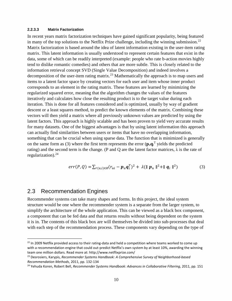
2.2.3.3 Matrix Factorization
In recent years matrix factorization techniques have gained significant popularity, being featured
in many of the top solutions to the Netflix Prize challenge, including the winning submission.22
Matrix factorization is based around the idea of latent information existing in the user-item rating
matrix. This latent information is usually understood to represent certain features that exist in the
data, some of which can be readily interpreted (example: people who rate b-action movies highly
tend to dislike romantic comedies) and others that are more subtle. This is closely related to the
information retrieval concept SVD (Single Value Decomposition) and indeed involves a
decomposition of the user-item rating matrix.23 Mathematically the approach is to map users and
items to a latent factor space by creating vectors for each user and item whose inner product
corresponds to an element in the rating matrix. These features are learned by minimizing the
regularized squared error, meaning that the algorithm changes the values of the features
iteratively and calculates how close the resulting product is to the target value during each
iteration. This is done for all features considered and is optimized, usually by way of gradient
descent or a least squares method, to predict the known elements of the matrix. Combining these
vectors will then yield a matrix where all previously unknown values are predicted by using the
latent factors. This approach is highly scalable and has been proven to yield very accurate results
for many datasets. One of the biggest advantages is that by using latent information this approach
can actually find similarities between users or items that have no overlapping information,
something that can be crucial when using sparse data. The function that is minimized is generally
on the same form as (3) where the first term represents the error (puqiT yields the predicted
rating) and the second term is the change. (P and Q are the latent factor matrices, λ is the rate of
regularization).24
𝑒𝑟𝑟(𝑃, 𝑄) = ∑ (𝑟𝑢𝑖 − 𝒑𝑢𝒒𝑖𝑇)2 + 𝜆(∥ 𝒑𝑢 ∥2+∥ 𝒒𝑖 ∥2)𝑟(𝑢,𝑖)∈𝑅 (3)
2.3 Recommendation Engines
Recommender systems can take many shapes and forms. In this project, the ideal system
structure would be one where the recommender system is a separate from the larger system, to
simplify the architecture of the whole application. This can be viewed as a black box component,
a component that can be fed data and that returns results without being dependent on the system
it is in. The contents of this black box are will themselves be divided into sub-processes that deal
with each step of the recommendation process. These components vary depending on the type of
22 In 2009 Netflix provided access to their rating-data and held a competition where teams worked to come up with a recommendation engine that could out-predict Netflix’s own system by at least 10%, awarding the winning team one million dollars. Read more at: http://www.netflixprize.com/ 23 Desrosiers, Karypis, Recommender Systems Handbook: A Comprehensive Survey of Neighborhood-based Recommendation Methods, 2011, pp. 132-134 24 Yehuda Koren, Robert Bell, Recommender Systems Handbook: Advances in Collaborative Filtering, 2011, pp. 151

11
recommender system but generally include some preprocessing of the data, an algorithm that
connects or groups either users or items and finally some method of drawing recommendations
from the calculated similarities.25
2.3.1 Data Preprocessing
There are very few cases where data can be read from a system and used as-is in a recommender
system. For the most part some logic is required to have the data make sense from an algorithmic
standpoint.26 Sometimes it is as simple as translating a dataset of likes and dislikes into 1’s and
0’s and sometimes it can be something requiring very complicated logic, e.g. data mining
operations such as clustering entities before using a neighborhood-based method or sampling
data to reduce computational cost.
There are many preprocessing schemes designed to cluster, classify or otherwise make sense
of the data before it being used by the recommender. Apart from these methods are the more
direct normalization measures that are applied directly on the ratings in order to increase the
accuracy of the predictions that are to be made using the data. An example of this is subtracting
users’ mean ratings from all their ratings in order to account for differences in rating behavior.
For methods that use complex data, preprocessing can be very expensive, something that is
important to remember when choosing a recommender system. Consider for example a content-
based recommender that uses key words to recommend news articles. To search thousands of
articles for multiple keywords and create profiles for each item is a huge preprocessing job
compared to computing the similarity between two profiles once they are created.
2.3.2 Similarity Measures
Many recommendation algorithms make use of some type of similarity measure. The common
collaborative filtering methods use similarities to first decide the top-N neighboring users or
items and then again to weigh the “importance” of the input from each of these neighbors (the
w’s in (1) and (2)). Text based systems often use cosine, or lexical, similarity to compute the
similarity between for example articles or reviews.
There are a number of common similarity measures, each with different pros and cons. Two
of the most common ones are the above mentioned cosine similarity and another called Pearson
correlation. Cosine similarity was first popularized in the field of information retrieval and is
defined as the cosine value of the angle between two rating vectors in n-dimensional space where
n is the number of elements in the vectors. For example, when computing the similarity between
two users in a movie rating database, n will be the total number of movies in the database.27
25 Desrosiers, Karypis, Recommender Systems Handbook: A Comprehensive Survey of Neighborhood-based Recommendation Methods, 2011, pp. 121-131 26 Xavier Amatriain, Alejandro Jaimes, Nuria Oliver, and Josep M. Pujol, Recommender Systems Handbook: Data Mining Methods for Recommender Systems, 2011, pp. 40-41 27 Desrosiers, Karypis, Recommender Systems Handbook: A Comprehensive Survey of Neighborhood-based Recommendation Methods, 2011, pp. 124

12
𝑐𝑜𝑠(𝐱, 𝐲) = (𝐱⋅𝐲)
∥𝐱∥∥𝐲∥ (4)
Pearson correlation measures the linear relationship between the same two vectors. This is done
by dividing the covariance between the vectors by the product of each vectors standard deviation
as shown below. 28
𝑃𝑒𝑎𝑟𝑠𝑜𝑛(𝐱, 𝐲) = ∑(𝐱,𝐲)
𝜎𝐱𝜎𝐲 (5)
Pearson correlation accounts for the mean and variance caused by differences in user behavior.
This is problematic when using implicit ratings. Accounting for the mean in a rating vector is
done by subtracting a user’s mean rating from each rating made by that user. When applying this
on implicit ratings the issue becomes that relatively low magnitude preferences are seen as
negative in comparison to the mean which does relay actual behavior well. A newer, more novel
similarity measure called inner product similarity has been suggested as a way of better capturing
similarities based on implicit ratings, as described below in (6).29 It is defined simply as the inner
product between two rating vectors. The idea is that when it comes to implicit ratings one might
not want to normalize the magnitude of the data by user behavior as in the other similarity
measures, since it can contain information. Instead the ratings are used as-is. The risk in doing
this is of course that very active users or users with very abnormal behavior might influence the
recommendations greatly.
𝐼𝑃(𝐱, 𝐲) = 𝐱 ⋅ 𝐲 (6)
2.3.3 Predicting and Recommending
The final step of the recommendation process is the recommending itself. This is sometimes
fairly trivial but can also turn into an involved process in its own right depending on the system
in question.
A recommendation is in most cases the direct product of a prediction. The system predicts
either the exact rating a user is likely to assign an item or simply a binary attribute such as
“might interest the user” or “probably not interesting to the user”. In some algorithms the
predictions are produced automatically, for example in the case of matrix factorization
algorithms the entire user-item rating matrix is filled with predicted values where there used to
be unknowns. In other algorithms each prediction has to be computed individually. This is the
case for user- or item-based methods where the predictions are drawn from an aggregate list of
neighbors’ rating histories. This calculation can be augmented by a variety of extra steps to
account for special attributes the data might have.
28 Desrosiers, Karypis, Recommender Systems Handbook: A Comprehensive Survey of Neighborhood-based Recommendation Methods, 2011, pp. 125 29 Tong Queue Lee, Young Park, Yong-Tae Park, A Similarity Measure for Collaborative Filtering with Implicit Feedback, Springer-Verlag Berlin Heidelberg, 2007

13
3 System Information This section will provide information about e-marketplaces in general and the Plick case
specifically. Its architecture, features, usage and data collection will all be described.
3.1 Data in the E-Marketplace
E-marketplaces have been around in some shape or form since the 90s and the concept is now far
from novel. Indeed it has now become a key part of the online market with businesses like eBay,
Craigslist and Etsy logging huge amounts of traffic and financial transactions. When considering
these sites it is important to remember that they are fundamentally different from regular e-
commerce sites such as Amazon (or really any retailer’s online shop). The most important
difference is the fact that in the e-marketplace the goods are being sold by users rather than the
provider of the system as is the case for regular e-commerce sites. This fact has a huge impact on
what kind of data can be collected for a recommender system. To understand what kind of data is
available we have to account for the following:
Every item in the system is unique (and even if they are not, it has to be assumed that
they are). This has huge implications in terms of what data can be known about each
item. There will be no historical data for purchases of the item, seeing as it disappears
from the system once it is sold. Furthermore, we will lack solid historical data for the
item in general. Page views, comments, likes, etc. mostly make sense after a certain
period of time when enough data has been built up to rule out anomalies and outlier-
behavior. Finally there is the fact that explicit ratings make almost no sense when items
can only be purchased once. Only in the sense that users browsing the item like the
pictures or description of it can explicit interest be collected, not in the sense of a review
given by an owner of the item.
Items are uploaded and described by each individual seller. This can lead to huge
differences in the quality of the description and what kind of information is available
about the item. Some users might provide every piece of information they can think of
whereas others might just say “worn once, buyer pays for shipping”. When this is the
case it can make it very difficult for any type of content-based system to find a
standardized way of comparing items. It is possible to guard against this however, mainly
by requiring users to provide certain pre-defined points of information about what they
are uploading.
The uniqueness of the items causes issues in the user-related data as well. Purchase
histories become shaky if a high percentage of transactions take place outside of the
system, a high throughput of items might lead to users missing items they would have
been interested in which risks skewing the data.
3.2 The Plick Case
Plick was first launched in 2013 and has since grown into a service with thousands of users and
tens of thousands of articles of clothing.

14
3.2.1 System Architecture
The main concept in the architecture of Plick is the focus on feeds. All clothes that are posted
can be seen in a “never ending” feed of pictures which is ordered by upload time, showing the
newest items first. This feed can be filtered in by gender, category and geographical location.
Additionally there is a second feed where items posted by users that you (as a user) follow are
shown. To interact with sellers, users can start conversations that are tied to each item where they
can work out purchase details, shipping and other practicalities.
This type of architecture has important effects on how users browse items. Both the follow-
feed and the browse feed show the newest items at the top, meaning that older items are pushed
down further and further as new items are uploaded. After time an item will only be found by
browsing for a relatively long time, alternatively by filtering the feed heavily to reduce the
amount of items shown. This means that items have a measurable life-span which is the period in
which they are viewed regularly and interacted with. Not only is this a strong argument for the
implementation of a recommender systems but it is also a reminder that items might be
overlooked by users for no other reason than that they did not use the app for the time a
particular item was “active”. This has important consequences for the selection of the
recommender system and will be covered in the next section.
Fig 2: The “Explore” view where most of the browsing happens.

15
Fig 3: The “home feed” where ads posted by people you follow are shown.
Fig 4: An individual ad’s page.

16
3.2.2 Features
Plick has a light-weight and minimalistic approach to e-commerce, e.g. the main browse-feed
contains nothing but pictures of items and only displays other information when a user clicks
through to an item’s page. Still, Plick does contain some essential features. There is a guide that
tells users how to upload their own items just using the camera on their phone. This guide also
gives tips about how to make sure that the item stands out and is displayed in the best possible
way. As stated above, users can “follow” other users which means that they subscribe to updates
about those users’ activities. Additionally, Plick is connected to Facebook and it is possible for
users to create their accounts through Facebook and also to share their ads on Facebook directly
through Plick. A user can also “like” an item when on the item’s page.
3.2.3 Users and Items
Users and items in Plick have a couple of different attributes connected to them. Users have a
name, email, country, city and description tied to them but everything is user-defined and except
for name and email they are optional, making the information known about one user very
different from the next. The items have more information tied to them. Seller, location and price
are all required to post an item to the system. Additional information consists of gender, size,
description but these are not required.
There is a clear division of users into three groups: buyers, sellers and people who do both.
The largest group is the buyers but many people do try to also sell items, although more
sporadically than the more specialized sellers. In this group we find a set of very active
individuals and another set of physical retailers who use Plick to advertise and sell part of their
inventory.
Plick is mostly a Swedish phenomenon as of now, with large clusters of users in the four
largest cities in Sweden. Little is known about what happens offline when a transaction is
initiated in the app. Payment- and shipping methods are mostly unknown and it is not possible to
track which user buys a certain item as both the financial and physical transaction happen outside
of the app.
By using the information about gender provided with the items it was possible to approximate
the ratio of female to male users and it was found that the number of female users far exceeds the
number of male users, something that also becomes apparent when scrolling through the app.
3.2.4 Data
With this information in mind we now know what kind of data that can be mined from the
system. It is obvious that a lot of the data in the system is unreliable, either because the users are
not required to provide it or as a result of the design of the system’s structure. This affects which
recommender system methods can be used and what kind of accuracy can be expected. There are
no explicit ratings except for likes, which are used by a subset of users. In terms of reliable
implicit data there are a few data points in the system that can be of use. Conversations between
buyers and sellers are strong indicators of interest and since they are the first step towards a

17
transaction they can be considered the closest thing to purchase history that is available. Another
key data point is item views. Whenever a user taps on an item’s image through to the item’s page
it indicates a certain interest in the item since the user selects the particular item out of a constant
flow of others. At the start of the project this user-action was not logged by the system but that
was implemented shortly after the beginning to facilitate the recommender system.
Even with item-views being logged, the data in Plick is very sparse. When the user-item
rating matrix is constructed this becomes very clear, having a 99.6% sparseness. However, it is
important to remember that this matrix includes many items that were uploaded long before
view-tracking was implemented and therefore has very few views since their time of activity is
long gone. The sparseness should decrease over time but will remain generally very high for a
data set of this type. To improve the data density during testing only data logged after the
introduction of view-tracking were used in this project.
4 Selecting a Recommender System So far we have discussed the most popular types of recommender systems. This section will
cover the reasoning and strategy behind selecting the components of a recommender system that
works for the e-marketplace case. To do this we must first understand the unique attributes of
Plick as an e-marketplace and how its features affect which methods can be implemented.
4.1 Matching Data and Algorithms
The data available in Plick renders certain recommender system methods unusable for this case.
Others are usable but may need tweaking. This section covers the reasoning behind the selection
of methods to implement and evaluate based on what was learned about the available data in the
previous section.
4.1.1 Content-based methods
The content available in Plick could theoretically be used to make recommendations. In practice
the huge difference in how extensive and detailed the content is makes it very hard to use a
standardized way of translating the content into numerical vectors and measuring them to each
other. There would essentially be two options to choose from when doing this. Either the vectors
are used as-is, meaning that the items with the most extensive information would be dominate
even if they only partly match a profile, leading to skewed recommendations. The second
approach would be to normalize all ratings into the same range, regardless of how many attribute
vectors are defined. This means that each item would have a certain level of uncertainty
connected to it, based on how many of the item’s attributes are defined which in turn would
make the user-profiles based on those items poorly defined as well. In the end it would mean that
different users would receive recommendations that were based on information of differing
quality. It would also mean that certain items could only be recommended with a limited amount
of certainty.
Content-based methods were quickly ruled out as a possibility for the above reasons but also
because of its computational cost. Considering how sparse the data is, the available item

18
descriptions would almost definitely be used. This would involve a keyword search and match in
order to make use of them, something that could become very computationally expensive.
4.1.2 Knowledge-based methods
Knowledge based methods were never really considered for Plick for a number of reasons. The
need for detailed information about users and about every individual item posted would require a
lot of attention and time from the users and would thereby increase the threshold for creating and
using an account in the app. Furthermore it could be argued that there is very little to be gained
by knowledge-driven, super accurate recommendations when it comes to clothes and accessories.
After all, a t-shirt is not an apartment and there is probably no singular item that is “perfect” for
any one user. The goal of a recommendation service for clothes is more along the lines of finding
items that are of the size, category and style that a user is interested in rather than their ideal
piece of clothing, which for many people might not even exist.
4.1.3 Collaborative Filtering methods
From the very beginning of the research phase of the project it became clear that collaborative
filtering would be the most viable approach for the project. Not only is it the earliest, most
widely adopted approach for recommender systems out there, collaborative filtering methods
also include the most cutting-edge algorithms currently used today in huge online systems such
as Amazon, Netflix, Spotify and Etsy. This fact has had an interesting effect on the research
being done on recommender systems. A lot of attention has been given to improving the
predictions made by collaborative filtering systems, both within the industry but also in
academia. An example of this is the research being done on matrix factorization methods in
connection to the Netflix Prize competition in 2009 where one such method was part of the
winning system and where many notable recommender system researchers participated.30 After
that, Spotify adopted a similar system, based on the research that was carried out during and after
the competition.31
The issues facing a collaborative filtering approach have mainly to do with three things:
Availability of historical data: This is the well-known “cold-start” problem that
collaborative filtering methods suffer from. It means that the entity focused on by the
algorithm is poorly defined until a certain amount of data has been built up.32 For
example, before a user has rated at least a few movies on Netflix it is impossible to say
anything about that user’s preferences. Conversely, a movie cannot be compared with
other movies in users’ rating histories if the movie has not been rated by anyone. In Plick
this problem is present but not insurmountable. By using the most basic action a user can
take (viewing item pages), data can be collected quickly and without any complex user
30 Grand Prize awarded to team BellKor’s Pragmatic Chaos, http://www.netflixprize.com/community/viewtopic.php?id=1537, 2009 31 Christopher C. Johnson, Logistic Matrix Factorization for Implicit Feedback Data, Stanford, 2014 32 Desrosiers, Karypis, Recommender Systems Handbook: A Comprehensive Survey of Neighborhood-based Recommendation Methods, 2011, pp. 131

19
input like explicit ratings which can be connected to a certain “maturity” of the user in
the system.
Sparseness of data: With the number of items in the tens of thousands, it is highly
unlikely that users have interacted with more than a couple of hundred at the most. As a
result, the user-item rating matrix is largely empty and yet this is all we have to work
with in a collaborative setting. This problem is present in most systems and Netflix
reports a similar level of sparseness as Plick.33 Data sparseness is a reality of the system
that cannot be avoided but is expected to improve over time as more data is collected
(remember that the item-viewing data has only been collected since the beginning of this
project). The main effect of a sparse user-item rating matrix is lowered accuracy of
predictions.34 A more active user will create a larger base of implicit data, containing
fewer cases of deviating behavior which allows for a better approximation of the user’s
actual preferences.
The burying feed: This issue is mostly specific to the e-marketplace case. It can be
assumed that in an e-marketplace the number of items in the system will increase steadily
with the number of users since it’s unlikely that all of them will be sold. The problem is
that if the method for displaying the items uses a continuous feed structure then there is a
risk that users will miss items that are added when they are inactive, especially if they
only use the service sporadically to begin with.
The impact of the burying feed can be mitigated by filtering but will still be a factor in
any subset of items that are sorted chronologically. Interestingly, one of the best ways of
combating this issue is by recommending items regardless of chronological data, meaning
that this problem should be alleviated by the introduction of a recommender system. The
recommender system would affect the data it is itself using to broaden the interaction
scope for users, bumping up older items and putting them back into circulation. This is
one of the main benefits of recommender systems.
Closely connected to this problem is the problem of older items that lack view-data and
are unlikely to be found by users and introduced into the recommender system. There is
no straight forward solution to this problem. Artificially assigning them views is not
possible since item-views are linked to a user and would introduce extreme skewing into
the data. The only mitigating circumstance in the case of Plick is that a couple of other
data points (likes, conversations) have been collected since the inception of the system
and thus some of these items have a chance of being “activated” by the recommender
system.
4.1.3.1 User-based
User-based collaborative filtering seemed to fit Plick well, both in terms of available data and in
terms of the system’s architecture and features. It especially seemed to suit the relationship
between items and users in the system. Contrary to the classical e-commerce case, the more
33 Yehuda Koren, Robert Bell, Recommender Systems Handbook: Advances in Collaborative Filtering, 2011, pp. 148 34 Desrosiers, Karypis, Recommender Systems Handbook: A Comprehensive Survey of Neighborhood-based Recommendation Methods, 2011, pp. 131

20
stable group in an e-marketplace is users rather than items. That means that users will have more
extensive historical data connected to them seeing as they are in the system indefinitely whereas
an item will with time be either sold or “forgotten” by the majority of the users. Users who have
been in the system for a while will have viewed a multitude of items and might also have
interacted with some of them through Facebook-sharing, likes or even conversations with the
sellers. All of these activities leave clues about the users’ interests and tastes which allows us to
compare and cluster them based on how similar their tastes are. Of course, new users will be
tough for the system to handle (the cold start problem described above). With only few items
interacted with (picked out of a small subset from the top of the feed) the new users will have
highly questionable behavioral data connected to them. There is a question of how well an
approach like this would scale. Computing similarities based on the entire set of items for
∑ 𝑛 − 1𝑁𝑛=1 user-pairs is not nothing.
4.1.3.2 Item-based
Using an item-based approach was definitely possible since the system could to a certain degree
be regarded as a traditional e-commerce case. Item similarities obviously occur in real life and
should be possible to find using user-item interaction data in a reversed fashion from the user-
based approach. That is, by looking at how many users an item has in common with another item
their similarity can be computed. However, the transient nature of unique second hand items
bring the correctness of these similarities into question. As an example: Calculating the similarity
between a popular and an unpopular item might often result in a high degree of similarity seeing
as the unpopular item will only have been viewed a few times and popular items are likely to
have those viewers in their own history. This risks creating false positives between unpopular
and popular items. As with most recommendation problems, an increase in data will fix this
problem of correctness. The issue is that there is no guarantee that this will happen since items
are added to the system continuously and so a large portion of them are always new (which can
be considered equal to being unpopular as far as the recommender is concerned).
4.1.3.3 Matrix Factorization
Matrix factorization techniques are difficult to theorize about without testing them because of the
complexity of the computations in the algorithm and the hidden nature of user- and item-factors.
On paper a correctly built and tuned matrix factorization algorithm should produce good
prediction accuracy in Plick. The sparseness in the user-item rating matrix is a similar level to
what Netflix reports and items as easily categorized as clothes should have plenty of latent
factors. The issue that a matrix factorization method could run into is the same as for most
methods, the problem of sparse data for new items. As stated before, this is a problem inherent in
the system. However, there is reason to believe that matrix factorization would handle this
problem better than other methods, mainly because of the concept of latent factors but also
because matrix factorization techniques are trained to fit the data, allowing for tailored
parameters that hopefully capture hidden information about the data.
The problem with this is that implementing and evaluating a matrix factorization technique is
time consuming and difficult. First, a complicated function describing the user-item rating
factors has to be defined, complete with parameters adjusting things like rate of convergence.
Then the unknown model parameters need to be learned by the system. This is done by
21
minimizing the function using an optimization technique, usually alternating least-squares or
gradient descent search. Both of these alternatives involve complexity and are computationally
expensive, making the implementation process a slow affair.
4.2 Implementation and Evaluation of Candidate Algorithms
Based on the knowledge we have of the available methods and the reasoning in the previous
subsection about possibility of matching methods with the Plick case, a few candidate algorithms
were selected for testing, namely item- and user-based collaborative filtering and also matrix
factorization. The selection of only collaborative filtering methods should at this point not be
surprising when considering what type of data is available in Plick.
It is important to note that the algorithms that were tested in this stage were implemented in
their most basic form, with some improvements being introduced later in the testing phase but
most of them being added to the best-performing algorithm during final implementation. This is
because testing every single permutation of each algorithm and each conceivable extension is
simply unfeasible in a project of this scale. Instead, based on theoretical knowledge about the
possible extensions, the ones that were likely to have the same impact on the results no matter
the method in question were assumed to be safe to leave for later implementation in the final
algorithm.
The testing was carried out in the following manner:
The algorithms were implemented in the programming language Python using
“blueprints” found either in recommender systems literature or online in the form of blog
posts by developers involved in companies such as Netflix and Spotify.
It was decided that the recommender system would only consider users that had
interacted with 10 or more items in order to keep the sparseness of the rating matrix
under control.
In every step of the algorithms the value of the variables currently being calculated were
cross checked with simplified manual calculations done on paper to make sure that the
values made sense.
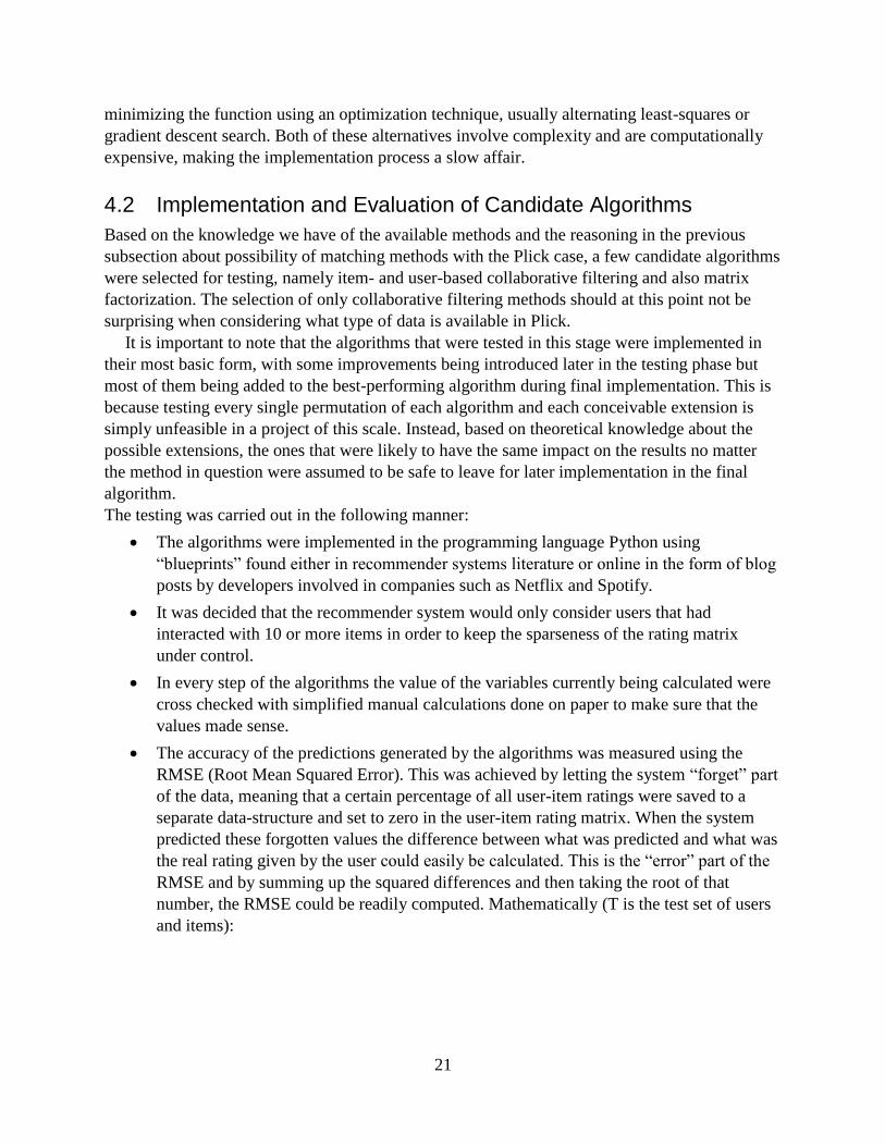
The accuracy of the predictions generated by the algorithms was measured using the
RMSE (Root Mean Squared Error). This was achieved by letting the system “forget” part
of the data, meaning that a certain percentage of all user-item ratings were saved to a
separate data-structure and set to zero in the user-item rating matrix. When the system
predicted these forgotten values the difference between what was predicted and what was
the real rating given by the user could easily be calculated. This is the “error” part of the
RMSE and by summing up the squared differences and then taking the root of that
number, the RMSE could be readily computed. Mathematically (T is the test set of users
and items):

22
𝑅𝑀𝑆𝐸 = √1
|𝑇|∑ (��𝑢𝑖− 𝑟𝑢𝑖)2
(𝑢,𝑖)∈𝑇 (7)35
In order to have a different measure to compare with, the MAE (Mean Absolute Error)
was also computed:
𝑀𝐴𝐸 = √1
|𝑇|∑ |��𝑢𝑖− 𝑟𝑢𝑖|(𝑢,𝑖)∈𝑇 (8)36
In addition to the above measures the results were also analyzed manually by spot
checking the top recommendations for some users and making sure that they made
somewhat sense to the extent that this was possible. This type of sanity check can be
surprisingly effective in ruling out potential changes to the system. Does it differentiate
between obvious groups such as men and women or are the recommendations mostly
random? Are the recommendations personalized or does everyone get the same set of
universally popular items recommended to them?
The testing as described in this report might seem linear and quite straightforward but this is only
how it appears when some coherence needs to be maintained, the truth is as always more
muddled and complex. There were in fact several rounds of testing for each algorithm.
Parameters, settings and the data pre- processing was changed several times during testing,
requiring many re-computations to maintain the exhaustive approach of the search. Before
getting into the testing of these algorithms we have to discuss which data was retrieved and how
it was converted into a format that could be used by the candidate algorithms, the step called data
pre-processing.
4.2.1 Data Selection and Preprocessing
As discussed in section 3.2.4 the only piece of explicit rating data in Plick was in the form of
likes provided by users on items. Seeing as likes are not on a scale and also sparsely used they
simply do not provide enough information to give any kind of clear picture of user interests.
Apart from these it became necessary to make use of implicit data. As a substitute for purchasing
history, the data on conversations was used to provide information about “purchase interest” and
the abundant item-views were used as an indicator of general interest in an item. The
conversation data was treated the same way as the like-data and put in a table containing user-
item pairs where each pair meant that a user had initiated a conversation about an item. The
view-data was considered in a similar fashion with the difference being that duplicates in this
table were summed up to the number of views by a user on an item. This was of course not
necessary in the case of the other data sets since in their cases each entry is unique.
There were essentially two ways of handling the collaborative data retrievable in Plick. Either
the different data-points could be handled separately, essentially running the algorithm as many
35 Desrosiers, Karypis, Recommender Systems Handbook: A Comprehensive Survey of Neighborhood-based Recommendation Methods, 2011, pp. 109 36 Ibid

23
times as there were different data sets and then merging the results of the separate runs at the
end, simply put a structure on the form: f(a) + f(b) + f(c). The other option was to merge the data
sets into a weighted aggregate before feeding it into the algorithm, making the algorithm a
unified function on the form: f(a, b, c). The benefit of doing so is that it would reduce complexity
and therefore running time but at the possible expense of information, seeing as the data sets
might contain different latent information.
For the first round of testing the second option was chosen. The reasoning behind this was
twofold. First, it is important to keep the running time to a minimum when running repeated
tests. Second, the conversation- and like-data sets are far sparser than the view-data which raises
the question of how much information could actually be lost by not considering them in their
own right. In the light of this it was decided that the data should be merged using a weighting
formula so that a user-item rating matrix could be constructed and fed to the algorithms as if it
contained one type of rating. (9) shows the structure of the formula (f is a function that caps the
impact of views on the final rating as they can be indefinitely many):
𝑟 = 𝑤1 ∗ 𝑟𝑙𝑖𝑘𝑒 + 𝑤2 ∗ 𝑟𝑐𝑜𝑛𝑣𝑒𝑟𝑠𝑎𝑡𝑖𝑜𝑛 + 𝑤3 ∗ 𝑓(𝑟𝑣𝑖𝑒𝑤) (9)
𝑟𝑙𝑖𝑘𝑒 , 𝑟𝑐𝑜𝑛𝑣𝑒𝑟𝑠𝑎𝑡𝑖𝑜𝑛 ∈ {0,1} 𝑟𝑣𝑖𝑒𝑤 ∈ [0, ∞)
𝑤1, 𝑤2, 𝑤3 ∈ ℝ
4.2.2 Item-Based
The implementation of the item-based method was mostly straightforward. It consisted of two
parts that each represented the two stages of collaborative filtering prediction, first a function
that calculated the item-similarities followed by a function that made predictions on a user-by-
user basis. The similarity function was implemented with a choice of two similarity measures:
cosine similarity and inner product similarity. Inner product similarity is a relatively new concept
in recommender systems but has been shown to improve similarities in some cases where
implicit ratings are used.37
These two similarity measures were very suitable for data represented on matrix form since
they both make use of the inner product between vectors without first manipulating them. This
means that it is simply a matter taking the dot product of the user-item rating matrix with its own
transpose to get these inner products. As an example let us say we have a set of four users and
four items, each of which have been rated by at least one user (remember, the actual user-item
rating matrix for Plick is much sparser than this example). In this case we end up with the
following:
37 Tong Queue Lee, Young Park, Yong-Tae Park, A Similarity Measure for Collaborative Filtering with Implicit Feedback, 2007

24
USERS
u1 u2 u3 u4
i1 3 1 3 0
ITEMS i2 5 0 3 0
i3 0 0 0 1
i4 1 2 3 5
ITEMS
i1 i2 i3 i4
u1 3 5 0 1
USERS u2 1 0 0 2
u3 3 3 0 3
u4 0 0 1 5
ITEMS
i1 i2 i3 i4
i1 19 24 0 14
ITEMS i2 24 34 0 14
i3 0 0 1 5
i4 14 14 5 39
Fig 5: Inner product similarity for items.
The inner product similarity measure is at this stage done and uses the values in the resulting
matrix. Cosine similarity includes one more step which is dividing these values by the product of
the magnitude of the vectors, thereby eliminating the influence of variance in the vectors. When
looking at the resulting matrix above it becomes apparent why this might make sense to do. It
appears that item 3 is more similar to item 4 than to itself (a value of 1 for itself as opposed to 5
for item 4 in the similarity matrix)! If we account for variance these values would instead be 1
and 5/11. This shows what strange things can happen if rating magnitudes are not normalized.
The second stage of this method is the prediction of user interest based on the similarity
between an item and a user’s “favorite” items. Since the goal is not to predict a certain user’s
interest in a certain item but all user’s interest in all items this becomes in practice very
expensive and the implementation only allowed for testing using a reduced test set size, about
25% of the actual data.
The results of the testing were very underwhelming. Not only was the RMSE very high, the
predictions were in a lot of cases zero. After debugging and evaluating each step of the algorithm
it became apparent that the sparseness of the data was a big problem for the item-based method.
The issue was identified as the lack of data shared between a target item (the item for which the
rating is being predicted) and the very limited set of rated items in the user’s history. Simply put
there seemed to be many cases where an item did not have a single user in common with the set
of items in the active user’s viewing history. When considering some of the attributes of the
system this is not very surprising. Consider the average case. The average user has only viewed a
small subset (in the order of ∼1%) of the items in the system. This means that the average item
has been viewed by an even smaller portion of users since there are more items than users. When
predicting the rating a user u is going to give an item i we want to take the ratings given by u to
the set Nu(i), items rated by u that are similar to i, and multiply them with the similarity between
i and the items in Nu(i). The problem is that in the set of ∼1% of items that the user has viewed,
the number of items with any defined similarity to i will be small and sometimes zero when the
data is this sparse. This comes from the fact that the average item only has views from one in a
hundred users, making it unlikely that it will have a user in common with any given item, the
basis for a similarity to be calculated. Even if it does have some defined similarities there needs
to be a certain number of them for all items since the item-similarities used should come from a
top-k selection from a sorted set Nu(i). When there are only a few defined similarities, the top-k
selection becomes the same as all defined similarities which makes the predictions very
●
=●

25
×
unreliable.
These issues could not really be handled by any change in the algorithm since they were a
direct effect of the data distribution in the system. As a result the item-based algorithm was
discarded in stark contrast to the common practice in the e-commerce field. In the recommender
systems literature it is generally considered wise to base predictions on the entity that has the
most data connected to it and it seems like this could be the reason why.
4.2.3 Matrix Factorization
The first thing to decide when implementing a matrix factorization algorithm is to either use a
pre-existing library of factorization functions or to define one yourself. The testing of matrix
factorization consisted of both of these approaches. First, a standard factorization function
(specifically a single value decomposition function) from the Python library Nimfa was
implemented and tested with the full Plick data set. The results were underwhelming. The
predicted ratings were very low and the only higher ones were for universally liked items,
indicating that the method had missed key latent factors.
The second attempt at matrix factorization therefore consisted of a custom made algorithm
that trained multiple latent factors, based largely on the method Simon Funk developed for the
Netflix Prize competition, together with a more simplistic algorithm from Albert Au Yeung at
Quuxlabs.3839
ITEMS
i1 i2 i3 i4
u1 r 0 0 0
USERS u2 0 r 0 r
u3 r r 0 0
LATENT
FACTORS
l1 l2
u1 l l
USERS u2 l l
u3 l l
ITEMS
i1 i2 i3 i4
LATENT l1 l l l l
FACTORS l2 l l l l
≈
ITEMS
i1 i2 i3 i4
u1 r' r' r' r'
USERS u2 r' r' r' r'
u3 r' r' r' r'
Fig 6: Decomposition of a user-item rating matrix into latent factor matrices.
38 Simon Funk, Netflix Update: Try This at Home, http://sifter.org/~simon/journal/20061211.html, 2006 39 Albert Au Yeung, Matrix Factorization: A Simple Tutorial and Implementation in Python, http://www.quuxlabs.com/blog/2010/09/matrix-factorization-a-simple-tutorial-and-implementation-in-python/, 2010
→

26
This approach allowed for better insight into each step of the algorithm and a better
understanding of what parameters were appropriate. The results from this implementation were
equally underwhelming but also came with some insight into the factorization process. Almost
all users were recommended the exact same items, mostly in the same order. However, the
predicted rating-scores differed wildly between users and seemed to be connected to the user’s
own rating behavior (active users with high rating scores received strong predictions, less active
users received lower). It seems like the user- and item-biases were not being handled well by the
algorithm. To combat this, baseline predictors were introduced. Baseline predictors could be said
to be crude predictions made purely from information about averages. They are found by
blending the average rating for a user with the average rating given to an item by all users. Thus,
there is a baseline predictor for each user-item pair. The effect of baseline predictors on the
matrix factorization method’s results were positive and did result in an improved RMSE-score
found when training 12 latent factors. The matrix factorization method’s ability to predict the
“forgotten” ratings was ultimately at a level that implied that the predictions made for unknown
ratings also should have decent accuracy. However, this is not necessarily the case. This will be
discussed at the end of this section.
4.2.4 User-Based
After having exhausted the two other collaborative filtering approaches with mixed results it
became clear that a user-based model not only made the most sense intuitively but also seemed
to be supported by lessons learned from the previous attempts. User-based filtering would focus
on the ratings collected for users and by doing so would avoid the crippling sparseness that
haunted the item-based approach as the average user has interacted with far many more items
than the average item has had users interacting with it. The questions that had to be answered
when implementing the user-based approach had mainly to do with the issue of computing
similarities and making sure that highly active users did not end up skewing results too much.
The same similarity measures that were used for the item-based approach were also used in this
approach. The idea is to calculate the similarity between all users and then by taking the top-k
most similar users for each individual, compiling lists of the nearest neighbors for each user. The
selection of these neighbors is very important for the accuracy of the predictions for a number of
reasons. Since the prediction for each item is a weighted sum of all of the ratings given by a
user’s neighbors, it is paramount that these neighbors are actually similar users and not just a
selection of active users that have interacted with some of the same items as the user by chance.
It is also important to note that the number of neighbors, k, is also very important. If too few
neighbors are used the predictions run the risk of becoming undefined because no neighbors have
interacted with a particular item. Furthermore, there is an issue of too much influence being
given to a small number of users which could lead to predictions becoming unreliable if some of
these similarities are high because of chance rather than real similarity. On the other hand, if too
many users are used as neighbors the risk is that predictions are made from more universal
agreement, leading to generalized recommendations rather than personalized ones. Simply put,
for this approach it is extremely important to tune the parameters right.
The similarities were calculated in the same way as for the item-based approach, simply by
computing the dot product of the user-item rating matrix with itself. From the resulting similarity

27
●
matrix a collection of users and their top-k neighbor-lists was compiled, containing the neighbors
id and the level of similarity to the user (to be used as a weight when predicting). The standard
way of producing recommendations from a collection like this would be to create a list of all
items that occur in the neighbors’ rating histories to be used as candidate items for prediction.40
In this case however it was of interest to predict all items in the system, mainly to be able to
compare the predictions for different algorithms and settings. It was also discovered to be faster
to simply compute predictions for all items rather than searching and compiling rated items into
lists for each set of neighbors, making any limitation on predicted items illogical. Thus the
structure of the algorithm came down to the following:
ITEMS
i1 i2 i3 i4
u1 3 5 0 1
USERS u2 1 0 0 2
u3 3 3 0 3
u4 0 0 1 5
USERS
u1 u2 u3 u4
i1 3 1 3 0
ITEMS i2 5 0 3 0
i3 0 0 0 1
i4 1 2 3 5
USERS
u1 u2 u3 u4
u1 35 5 27 5
USERS u2 5 5 9 10
u3 27 9 27 15
u4 5 10 15 26
↓
USERS
u1 u2 u3 u4
NEAREST u3 u4 u1 u3
NEIGHBORS u2 u3 u4 u2
u4 u1 u2 u1
Fig 7: Inner product similarity for users. The nearest neighbors are easily extracted in the last
step.
The first version of the user-based approach was simple but produced reasonable results. The
recommendations were however global rather than personalized and when looking at the nearest
40 Desrosiers, Karypis, Recommender Systems Handbook: A Comprehensive Survey of Neighborhood-based Recommendation Methods, 2011, pp. 115-116
=●

28
neighbors-lists it became apparent that a small number of super active users were dominating
predictions for nearly all users. This was to be expected as the basic implementation did not
contain any corrections for user-bias. A way of accounting for this would be to normalize the
ratings by subtracting a user’s mean rating from all of the user’s ratings.41 However, as described
in section 2.1.2, there is the issue of what happens to the lower than average ratings that suddenly
become negative in that scenario. As all implicit feedback should be considered positive, even if
it is lower than a user’s average interest, there is simply no good way of handling this kind of
bias and instead one has to properly cap the magnitude of ratings when the user-item rating
matrix is constructed so that “outlier behavior” is reined in before the similarities are computed.
This was an important tool when improving predictions for all algorithms and will be described
in section 4.3. It was however found that the cosine similarity measure produced more
personalized similarities which probably comes down to the fact that although it does not
account for differences in mean and variance of users, cosine similarity does account for the
magnitude of the rating vectors and will curb the impact of extreme user behavior somewhat.
4.3 Extensions and Improvements
This section describes the various extensions that were tested in order to improve the predictions
made by the candidate algorithms. It is important to note that not all extensions were applicable
to all three algorithms.
4.3.1 Rating Aggregation
The aggregation of the views, conversations and likes into unified ratings is one of the most
crucial components of this recommender system. Simply counting views as a binary data point,
viewed vs not viewed, might seem logical but would result in a huge loss of information if the
reality of user behavior is considered. Re-viewing the same item a couple or many times may
indicate a huge interest, especially when considering the concept of the burying feed described
earlier. A user that specifically seeks out the same item for viewing multiple times even when it
has been pushed down far in the feed indicates a significantly higher level of interest compared
to a single view on an item at the top of the feed. Another problem with this model is that the
relatively small subset of items that have likes or conversations connected to them will dominate
and skew ratings. On the other hand considering the number of views the same as likes and
conversations is also unreasonable as a user can have viewed the same item 40 times but can
only have liked or conversed about it once. There is need of a middle ground.
The formula that is proposed here is based on the following logic: likes and conversations
indicate a level of interest comparable to re-viewing the same item more than two times. One or
two views on the same item indicates a browsing preference, the item has been picked out and
clicked out of a set of many items. Re-viewing an item a couple of times indicates a stronger
preference and possibly an interest in purchasing the item. However, the impact of views on the
same item is curbed after this as there must be a maximum level of interest that can be
interpreted from a user viewing an item. Essentially, there should be no difference in the rating
41 Desrosiers, Karypis, Recommender Systems Handbook: A Comprehensive Survey of Neighborhood-based Recommendation Methods, 2011, pp. 121-122

29
given an item based on 20 views by the same user as compared to the rating given by 50 views,
both indicate a strong interest and the more extreme data should be understood as an expression
of anomalous user-behavior. Finally, there is need of a base rating value given to an item with a
single view that can be used as an easy controlling parameter for the interval of ratings and the
impact of views versus other data. With this reasoning the proposed structure for the rating
aggregation becomes:
𝑟 = 𝑤1 ∗ 𝑟𝑙𝑖𝑘𝑒 + 𝑤2 ∗ 𝑟𝑐𝑜𝑛𝑣𝑒𝑟𝑠𝑎𝑡𝑖𝑜𝑛 +∗ 𝑓𝑣𝑖𝑒𝑤𝑐𝑎𝑝(𝑟𝑣𝑖𝑒𝑤, 𝑤3) (9)
𝑓𝑣𝑖𝑒𝑤𝑐𝑎𝑝(𝑟, 𝑤) = 𝑤 + 0.5 −0.5
𝑟 (10)
With this formula the value of fviewcap will be bounded by its second and third terms which will
create the domain [w3, w3 + 0.5] for the view-part of ratings. Keeping in mind that likes and
conversations can take the values 1 or 0 this means that the maximum rating becomes w1 + w2 +
w3 + 0.5.
4.3.2 Rating Normalization
Despite the issues brought up in previous sections concerning rating normalization there was
some testing and investigating carried out in an attempt to fully exhaust the option of
normalizing ratings to account for user- and item biases. First, the previously mentioned Pearson
correlation was used as the similarity measure in both the user- and the item-based collaborative
filtering methods. The results produced by the user-based algorithm matched the results when
using cosine similarity but when taking a closer look at the recommendations given by the
algorithm it became clear that this measure did a much better job at blocking recommendations
made from low but broad support among the neighbors than it did limiting the influence of
highly active users.
Apart from the Pearson correlation there were also some attempts made to normalize ratings
before similarities were calculated. Subtracting mean ratings for both users and items and
capping negative ratings to 0 produced acceptable results but eventually led to similar loss of
information as when using Pearson correlation. It became apparent that fixed intervals and clear
bounds (as described in section 4.3.1) was the only way of maintaining a good balance between
the impact of few extreme ratings and many low ratings. This was further improved by
introducing significance weighting, described in 4.3.3.
4.3.3 Frequency Weighting
When trying to extract the most informative parts of a dataset it is important to account for
variance. In this case it can be understood as adjusting the impact of certain ratings on user-
similarities based on how much information the ratings are thought to provide.42 In practice this
means penalizing the impact of universally liked items and favoring less known items as it is
likely that two users having such an item in common in their rating history is telling of a greater
42 Desrosiers, Karypis, Recommender Systems Handbook: A Comprehensive Survey of Neighborhood-based Recommendation Methods, 2011, pp. 129

30
degree of similarity. This is done by applying a factor calculated as the log-ratio of users that
have rated an item as compared to the total number of users.
𝜆𝑖 = log|𝑈|
|𝑈𝑖| (11)
A good example of this is in movie ratings where high ratings given to a movie like The
Godfather are essentially disregarded as they are considered almost default. In the case of Plick it
became apparent that there exists a subset of very popular items that affect predictions negatively
and the introduction of frequency weighting reflected positively in the results when applied to
the user-based method and matrix factorization method.43
4.3.4 Significance Weighting
There have been a number of strategies suggested to account for the significance of a similarity,
either between two users or two items. The problem that these strategies are trying to solve is
that in a sparse environment it is not uncommon for two entities to have very little data in
common which can create situations were recommendations are unknowingly based on very
weak similarities.44 As an example, take two low- to medium active users in Plick. Say that they
have viewed only a few items each but have one item in common. Their similarity will be fairly
significant and they will probably have each other as neighbors in a user-based system.
Recommendations will then be made to both of them based on their respective historical
interactions with the items in the system even though their actual preferences may differ wildly.
The proposed solution to this problem is an intermediate step just after the similarity calculation
called significance weighting. The idea is very straightforward: if the number of commonly rated
items is below a certain threshold the weight will be penalized by a factor proportional to the
difference between the number of rated items in common and the threshold, as described in (12)
45 (for a user-based model, the wuv represents the similarity weight between users u and v, Iuv the
set of items u and v have both interacted with. γ is the threshold value):
𝑤′𝑢𝑣 = min{|𝐼𝑢𝑣|,𝛾}
𝛾∗ 𝑤𝑢𝑣 (12)
This strategy had a powerful impact on predictions and when examining the lists of neighbors
assigned each user it was found that they became more diverse in terms of activity and more
homogenous in terms of demographics, something that indicates real similarity in this context
(e.g. women have more in common with other women than men when it comes to clothing
preferences).
Still, significance weighting applied on similarities may have helped account for low
confidence neighbors but it did not address the issue of recommendations being made based on a
43 Ibid 44 Desrosiers, Karypis, Recommender Systems Handbook: A Comprehensive Survey of Neighborhood-based Recommendation Methods, 2011, pp. 127-128 45 Ibid
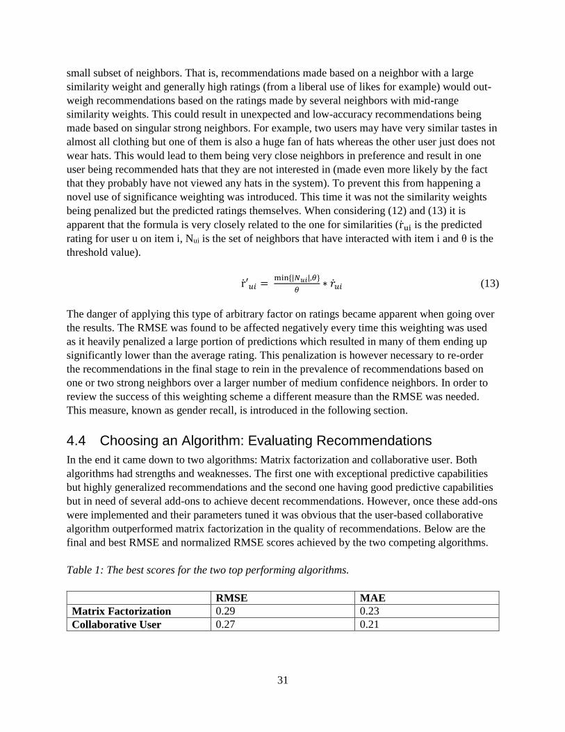
31
small subset of neighbors. That is, recommendations made based on a neighbor with a large
similarity weight and generally high ratings (from a liberal use of likes for example) would out-
weigh recommendations based on the ratings made by several neighbors with mid-range
similarity weights. This could result in unexpected and low-accuracy recommendations being
made based on singular strong neighbors. For example, two users may have very similar tastes in
almost all clothing but one of them is also a huge fan of hats whereas the other user just does not
wear hats. This would lead to them being very close neighbors in preference and result in one
user being recommended hats that they are not interested in (made even more likely by the fact
that they probably have not viewed any hats in the system). To prevent this from happening a
novel use of significance weighting was introduced. This time it was not the similarity weights
being penalized but the predicted ratings themselves. When considering (12) and (13) it is
apparent that the formula is very closely related to the one for similarities (rui is the predicted
rating for user u on item i, Nui is the set of neighbors that have interacted with item i and θ is the
threshold value).
r′𝑢𝑖 = min{|𝑁𝑢𝑖|,𝜃}
𝜃∗ ��𝑢𝑖 (13)
The danger of applying this type of arbitrary factor on ratings became apparent when going over
the results. The RMSE was found to be affected negatively every time this weighting was used
as it heavily penalized a large portion of predictions which resulted in many of them ending up
significantly lower than the average rating. This penalization is however necessary to re-order
the recommendations in the final stage to rein in the prevalence of recommendations based on
one or two strong neighbors over a larger number of medium confidence neighbors. In order to
review the success of this weighting scheme a different measure than the RMSE was needed.
This measure, known as gender recall, is introduced in the following section.
4.4 Choosing an Algorithm: Evaluating Recommendations
In the end it came down to two algorithms: Matrix factorization and collaborative user. Both
algorithms had strengths and weaknesses. The first one with exceptional predictive capabilities
but highly generalized recommendations and the second one having good predictive capabilities
but in need of several add-ons to achieve decent recommendations. However, once these add-ons
were implemented and their parameters tuned it was obvious that the user-based collaborative
algorithm outperformed matrix factorization in the quality of recommendations. Below are the
final and best RMSE and normalized RMSE scores achieved by the two competing algorithms.
Table 1: The best scores for the two top performing algorithms.
RMSE MAE
Matrix Factorization 0.29 0.23
Collaborative User 0.27 0.21

32
These scores only tell half the story. Something needs to be clarified about the RMSE. As this
measure is based around the squared error between prediction and reality it punishes large
differences significantly compared to smaller errors. This leads to a situation where, in terms of
RMSE, it is preferable to have four mediocre predictions rather than one perfect prediction, two
mediocre ones and one bad one. When considering that recommendations are delivered in top-10
lists it seems that it is less relevant how many mediocre recommendations there are further down
in the top-list as long as the top 10 recommendations are as good as they can be. The fact that the
matrix factorization algorithm will always predict all unknown ratings means that it will not
suffer any penalties in the RMSE for missing to predict a forgotten rating, a rather large penalty
as the squared difference between zero and a rating will be relatively big. Also, the RMSE is
based on the algorithms ability to predict a known subset of ratings that were intentionally
“forgotten” by the system. The logic is that if these real ratings are predicted accurately then the
predictions made for completely unknown items should also be accurate. Still, it is not a measure
of how good the actual recommendations are. The quality of the recommendations can only be
measured with some type of user feedback, something that was unavailable when this project
was carried out. Some type of approximation of user input was needed.
4.4.1 Gender Recall
The solution was found when going back to the other part of the data that was on hand, the
content. By matching a user attribute with an item attribute it would be possible to measure some
degree of qualitative accuracy in recommendations. That is if it was known about users what
their favorite colors were and the items were all color coded, then that could be used to check if
the recommendations made sense. In lieu of something that obvious the only data point that
could be used in this way was the gender. Specifically the substantial difference between male
and female users allowed for a type of sanity check of the top recommendations made to male
users. As the average male users rating history contained mostly male and unisex items it was
expected of the system to produce recommendations in these categories. This should be achieved
despite about 65% of items in the system being tagged as female, including the most popular
items. Under these circumstances it could be considered a decent measure of some basic
accuracy that the system can identify a user’s gender and recommend accordingly. Important to
note is that this is still not a real measure of user feedback like measuring click-through rates for
example. It also does not say anything about the actual taste of the user and how the
recommendations match that. The test function measured the percentage of items tagged as male
or unisex in the top 10 recommendations for a subset of male users. These users were manually
identified by username or email as the gender is not specified by users themselves. The
performance of the algorithms on this gender recall index is presented below.
Table 2: Best gender recall score for the two top performing algorithms.
Gender Recall
Matrix Factorization 38%
Collaborative User 74%

33
When taking these scores together it becomes obvious that the collaborative user algorithm is the
only one that can actually produce recommendations pertinent to each individual user. With this
evaluation done, the collaborative user algorithm was selected for implementation in the final
system.
5 Final System
5.1 Parameter Tuning
Optimal parameters for the collaborative user method were found in the last stage of testing
using a three dimensional grid search. Parameters were increased or decreased in different
permutations within certain viable value ranges found in earlier testing phases. When all
permutations were calculated the vertices defined by each combination of parameter values
formed a honeycomb-like structure in three-dimensional vector space. The cuboid in this space
containing the best target values would then become the next interval for another grid search,
thus “zooming in” on the optimal parameter values iteratively.46 The targets were RMSE and
gender recall and the variables were the number of neighbors and the threshold values for
significance weighting, both for low confidence neighbors and for low confidence
recommendations. This way of estimating parameters is not ideal and there are better ways of
minimizing functions but when considering the running time of just one round of the user based
method (~4 minutes) it is simply not feasible to use a strategy that requires thousands of
iterations.
5.1.1 Algorithm Parameters
Because of the three-dimensional nature of the target function during parameter optimization it is
difficult to convey graphically where the optimal parameters were found. We can however
represent the optimization process in two parts; the number of neighbors and the connected
significance threshold value with RMSE as a target and the low confidence prediction penalty
threshold. The first two parameters have the same target and can be represented graphically.
46 James Bergstra, Yoshua Bengio, Random Search for Hyper-Parameter Optimization, Journal of Machine Learning Research 13, 2012, pp. 281-305

34
Fig 8: The RMSE for different neighbor- and significance threshold-settings.
From Fig 8 it becomes apparent that a low RMSE (indicated by the grey area in the graph) is
achieved with an increasing number of neighbors. It can also be gleaned that a similar low
RMSE is achieved by increasing the significance threshold, almost regardless of the number of
neighbors more than 24. In recommender systems literature it is generally considered bad to use
more neighbors than necessary as recommendations taken from a large set of weak neighbors
will conform more and more to general opinion rather than personal opinion, resulting in non-
personalized recommendations.47 With this in mind the most interesting part of this grid becomes
the 24-36 span for the number of neighbors and a significance threshold value of between 12 and
20. Important to note is that although it is hard to see in the graph, the RMSE increases with a
significance threshold value over 20 which is why that is the upper bound for that variable in the
grid search.
Another view of this is presented in Fig 9. The series of graphs show the impact of the
significance threshold on the RMSE and it can be seen that the effects are similar almost
regardless of the number of neighbors.
47 Desrosiers, Karypis, Recommender Systems Handbook: A Comprehensive Survey of Neighborhood-based Recommendation Methods, 2011, pp. 131
0
4
8
12
16
20
0
0.1
0.2
0.3
0.4
0.5
0.6
0.7
1224
3648
60
Sign
ific
ance
Pe
nal
tyTh
resh
old
RM
SE
Neighbors
Target: RMSEVariables: Neighbors and Significance Threshold
0.2-0.3 0.3-0.4 0.4-0.5 0.5-0.6 0.6-0.7

35
Fig 9: The RMSE for five selections of the number of neighbors with different significance
threshold-settings.
Looking at the gender recall measure in the same intervals without the use of the confidence
penalty showed a recall of between 40% and 45% for all combinations of neighbors and
significance penalties. This is very close to the 38% percent achieved by the matrix factorization
method and does not reach very high in the interval between picking an item at random (35%
likelihood of it being male or unisex) and the average rating behavior of male users (about 74%
of items viewed by males are male or unisex). When introducing the confidence penalty the
impact is obvious as can be seen in Fig 10. The graph shows the average development of the
gender recall as a function of the confidence penalty threshold over the vertices in the first grid.
0
0.05
0.1
0.15
0.2
0.25
0.3
0.35
0.4
0.45
0.5
0 5 10 15 20 25 30
RM
SE
Significance Threshold Neighbors
Target: RMSEVariable: Significance threshold
25 30 35 40 45
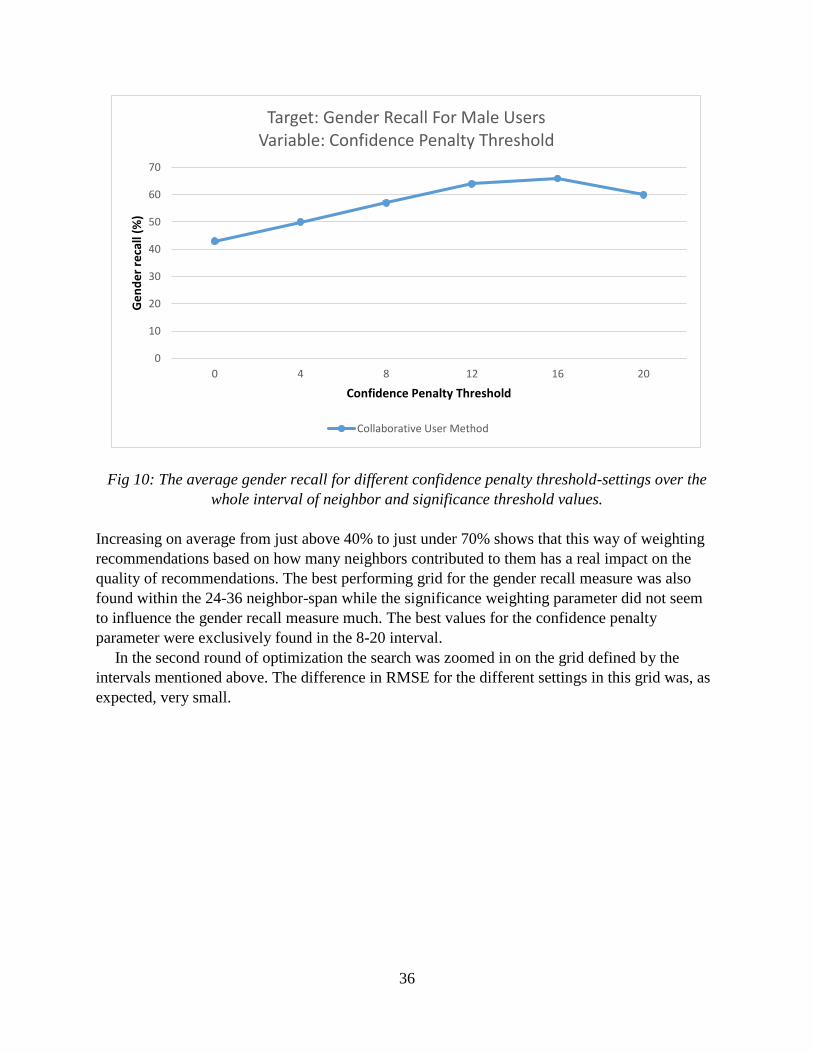
36
Fig 10: The average gender recall for different confidence penalty threshold-settings over the
whole interval of neighbor and significance threshold values.
Increasing on average from just above 40% to just under 70% shows that this way of weighting
recommendations based on how many neighbors contributed to them has a real impact on the
quality of recommendations. The best performing grid for the gender recall measure was also
found within the 24-36 neighbor-span while the significance weighting parameter did not seem
to influence the gender recall measure much. The best values for the confidence penalty
parameter were exclusively found in the 8-20 interval.
In the second round of optimization the search was zoomed in on the grid defined by the
intervals mentioned above. The difference in RMSE for the different settings in this grid was, as
expected, very small.
0
10
20
30
40
50
60
70
0 4 8 12 16 20
Ge
nd
er
reca
ll (%
)
Confidence Penalty Threshold
Target: Gender Recall For Male Users Variable: Confidence Penalty Threshold
Collaborative User Method

37
Fig 11: The RMSE for different neighbor- and significance threshold-settings in the zoomed in
grid.
Since the highest and lowest achieved RMSE scores only differed by ~0.04 it could be
considered that any combination found in this grid would be very likely to produce the same set
of top-k neighbors. Increasing the number of neighbors would likely only add low-similarity
users to the prediction, diluting the recommendations with input from low-significance
neighbors. This was further confirmed when looking at the MAE for the same grid. It showed
that the improvement gained by increasing the number of neighbors and the significance
weighting was miniscule (~0.01 change in the MAE) which implied that the slight improvement
in RMSE with more neighbors was simply very low confidence recommendations being made on
items that were not covered by the top neighbors but were rated by the user, resulting in a
noticeable difference in RMSE since the error caused by missing a rated item is rather large
when squared, regardless of what the recommendation is.
Finally, the gender recall measure in the same grid was found to reach a ceiling between 72%
and 78%. The fact that the gender recall could be brought above the average viewing behavior of
male users is not very surprising as the average rating given by a male user to a male or unisex
item is probably higher than for female items (i.e. a male user is more likely to like or start a
conversation about a male or unisex item), resulting in more gender-specific items in the top
recommendations. In Fig 12 the significance weighting parameter was fixed to 12 to allow the
other two parameters to be plotted as an area.
12
16
20
24
0.24
0.25
0.26
0.27
0.28
0.29
24 2628
3032
3436
Sign
fici
can
ce P
en
alty
Th
resh
old
RM
SE
Neighbors
Target: RMSEVariables: Neighbors and Significance Threshold
0.26-0.27 0.27-0.28 0.28-0.29

38
Fig 12: The gender recall for different neighbor- and confidence penalty threshold-settings.
From this grid search it could be deduced that the optimal parameters existed in the vicinity of
~26 neighbors, ~12 significance penalty threshold and ~14 confidence penalty threshold. Note
that these parameters did not yield the very best RMSE-score or the very best gender recall score
but did best overall, while minimizing the impact of the penalties on the scores which
theoretically should lead to the best balance between recommendations given by a small number
of high-similarity neighbors and recommendations given by a larger number of medium-similar
neighbors.
5.1.2 Rating Aggregation Weights
Since there was no user feedback to measure the success of the recommendations it was not
possible to optimize the weights given to the three data points used by the algorithm; views, likes
and conversations. Consider the measure with which two of the other parameters were
optimized, the RMSE. If the same logic was applied to optimizing the aggregation weights the
system would be changing both the recommendation value but also the value it was being
compared to since the whole rating matrix would be re-computed. In this scenario the optimal
weights would simply be zero since that would result in an error of zero.
That having been said, the weights were not chosen at random. Currently the system uses the
following weights: 2.0 for views, 0.5 for likes and 0.5 for conversations. These weights were
found through trial and error and are essentially at a rough balance between not letting the
relatively rare occurrence of a like or a conversation influence ratings too much while
maintaining the information provided by these two data points. Also remember that the views
8
12
16
20
40
50
60
70
80
90
100
2426
2830
3234
36
Co
nfi
de
nce
Pe
nal
tyTh
resh
old
Ge
nd
er
Re
call
(%)
Neighbors
Target: Gender RecallVariables: Neighbors and Confidence Penalty Threshold
40-50 50-60 60-70 70-80 80-90 90-100

39
can be many but are on a logarithmic scale that converges at about 2.5, making the maximum
possible rating ~3.5, occurring when a user has liked an item, started a conversation with its
owner and also gone back to view it again >10 times.
5.2 Schemas
5.2.1 Algorithm
Views, Likes, Conversations Recommendations
User-Item Rating Matrix User-Item Prediction Matrix
User-Item Rating Matrix User-Item Rating Matrix
Top-K Neighbors
User-Item Rating Matrix
User-Similarity Matrix
Plick
RatingAggregation
FrequencyWeighting
K-Nearest Neighbors
Confidence Penalization
Prediction
Significance Weighting
Fig 13: The structure of the final recommender algorithm.

40
5.2.2 System
Plick Recommender
MongoDBDatabase Plick API
USER USERUSER
Fig 14: The placement of the recommender system within the larger system.
6 Discussion and Conclusions When it comes down to it, the business of recommending things to people is more involved than
you might expect. In the age of big data and data mining the tools and methods used to make
sense of the behavior and opinions of everyone are getting increasingly complex. Even so, the
amount of data produced by people going about their daily digital routine leave even the most
high-end computing hardware playing a hopeless game of catch up in terms of processing and
analyzing.48 This requires smarter and more efficient algorithms which in turn means
approximations, simplifications and compromises. In the case of designing a recommender
system this means a trade-off between things like picture analysis and geo-tracking for
computational speed. Straightforward data such as likes, star-ratings and views become more
attractive in that they are simply numerical values right of the bat.
There is a second trade-off when designing a recommender system that is decided outside the
scope of the recommender itself which can be understood as a trade-off between usability and
information. That is, how much information is explicitly provided by users and how much can
you realistically ask for before it becomes a hindrance when using the system. A choice of a 5-
star rating next to a movie in Netflix is a far cry from a filling out a compulsory form explaining
exactly what you liked about the movie after watching it. That would however allow for
exceptionally accurate recommendations. With Plick the main idea has always been to allow
users to post their clothes quickly and without any hassle which means that the explicitly given
information is sparse and recommendations need to be based mainly on whatever implicitly
provided data that is available. Earlier it was established that implicit data can represent different
preferences compared to explicit data. On the one hand explicit ratings have a very clear
48 The Economist, Data, data everywhere, 27-02-2010
41
meaning but users might be hesitant to provide explicit ratings for every part of their preference.
Comparatively, implicit ratings will in an ideal world show the true preference of the user as it
monitors actual behavior. The risk when using this data is of course that a lot of this behavior
might not be indicative of any particular preference and that any hidden patterns remain unfound.
In Plick it remains largely unknown what is actually observed in the user-logs but as shown in
the results in the previous section, the ability to produce a portion of predictions with a matching
gender larger than what a random selection of items would yield demonstrates that there is some
degree of information about actual preferences in the logs.
The challenges of recommending in an e-marketplace environment posed in the beginning of
this report were met and to some degree dealt with during the process of testing and tuning the
different candidate algorithms. The algorithms tested during this project did not exhaust the
multitude of methods that have been explored in recommender systems research in recent years,
but it did touch upon most of the major approaches used today. Entire categories such as
knowledge-based and content-based systems were quickly dismissed based on the data available.
The item-based method could have been dismissed for similar reasons but was considered
interesting to evaluate as a way of confirming the idea that the relationship between items and
users in a system decides which entity to base recommendations around. It was found that this is
at least true for a system like Plick, as the item-based method produced essentially undefined
results and the user-based method was the best performing one. While it this find cannot be
extrapolated over the whole e-marketplace sector it is a clear indication that quite contrary to the
standard e-commerce scenario, the e-marketplace revolves around users. There is every reason to
believe that if the content is sparse, there is no explicit rating system and the items in the system
have a short lifespan then the best choice for a recommender system is a user-based collaborative
method based on implicit user feedback like the one presented in this report. The data necessary
for a system like this should in most cases be available as most environments where users both
buy and sell items requires users being logged into an account when using the system. However,
to make sure that a system of this type is sufficiently accurate there is a need to alpha and beta
test recommendations to collect user feedback. Advisable would be to use a scheme of
displaying random items in one view and recommended items in another to measure how well
the recommendations outperform lazy browsing behavior. It was not possible to carry out such a
test during this project which meant that the results existed in a kind of darkness were the user
was left out of the loop. This further meant that weights deciding the impact of different data
types could not be optimized. In general, optimizing the impact of different types of data to
construct singular user-item ratings is something that has been mostly overlooked in
recommender system research; at least in what was covered in this project’s literature study. As
it stands they could probably most easily be found in a very late stage of testing by observing
changes in the click-through rate for recommendations while adjusting the weights.
In contrast to what was learned about the effectiveness of user-based collaborative filtering
over item-based, the appropriateness of matrix factorization methods for marketplace-
applications is still a big question mark. Where the item-based method failed because of its most
fundamental attributes, the matrix factorization method failed for reasons not well understood.
One explanation might be the complexity of the approach. Where the other collaborative filtering
algorithms are intuitive and easy to follow, the matrix factorization techniques are, apart from the

42
most simplistic versions (like the one implemented here), very intricate and often involve
multiple stages of calculation and re-calculation of large data structures. There is no doubt that a
system of that caliber would perform very well in an application like Plick. Another reason might
be a stronger sensitivity to the weighting of the data points. It is possible that the boost in scores
for items that had been liked or conversed about over those that had not was not adequately
addressed in the algorithm used in this project.
The issue of new users was unsurprisingly not completely resolved. The final system could
not handle brand new users but seeing as the testing incorporated users with an interaction
history of as few as ten items and still achieved decent results, there seems to be something to be
gained by using such a fundamental statistic as a click to build recommendations from. Page
views build up incredibly fast in almost any system and making use of that resource as a way of
handling cold-start issues is something that deserves more attention. When it comes down to it, it
is actually a very minor problem that users who have not clicked more than ten ads are not given
recommendations; if they are that inactive, why would they be interested in personalized
recommendations anyway?
One of the major limitations of the project was the lack of data about usage and feedback
from users themselves. Obviously, this could not be helped since the recommender system was
not implemented into the live system during the course of the project. Going forward however,
the system is to be deployed in the first half of 2015 which will allow for additional testing and
tuning of the collaborative user algorithm and its parameters. The increasing number of users and
activity in Plick will provide denser data and it will be interesting to see how this will affect the
quality of recommendations. As the application is developed, more types of data will become
available which will allow for the recommender system to be further developed as well.
Incorporating things like categories or brands by making the algorithm a content-
based/collaborative filtering hybrid could certainly add another level of ingenuity to the system.
Remember, if the processing power is there, you can never have too much information in a
recommender system.

43
7 References
Books
[1] Francesco Ricci, Lior Rokach, Bracha Shapira, Paul B. Kantor [editors], Recommender
Systems Handbook, Springer, 2011
[1.1] Francesco Ricci, Lior Rokach, Bracha Shapira, Introduction to Recommender
Systems Handbook
[1.2] Xavier Amatriain, Alejandro Jaimes, Nuria Oliver, and Josep M. Pujol,
Recommender Systems Handbook: Data Mining Methods for Recommender Systems,
2011
[1.3] Christian Desrosiers, George Karypis, Recommender Systems Handbook: A
Comprehensive Survey of Neighborhood-based Recommendation Methods
[1.4] Yehuda Koren, Robert Bell, Recommender Systems Handbook: Advances in
Collaborative Filtering
[1.5] Alexander Felfernig, Gerhard Friedrich, Dietmar Jannach, Markus Zanker,
Recommender Systems Handbook: Developing Constraint-based Recommenders
[2] Dietmar Jannach, Markus Zanker, Alexander Felfernig, Gerhard Friedrich, Recommender
Systems: An Introduction¸ Cambridge University Press, 2011
Research Papers
[3] Tong Queue Lee, Young Park, Yong-Tae Park, A Similarity Measure for Collaborative
Filtering with Implicit Feedback, ICIC 2007, LNAI 4682, Springer-Verlag Berlin Heidelberg
[4] Peter Vojtas, Ladislav Peska, Negative Implicit Feedback in E-commerce Recommender
Systems, Proceedings of the 3rd International Conference on Web Intelligence, Mining and
Semantics, Article No. 45, 2013
[5] Christopher C. Johnson, Logistic Matrix Factorization for Implicit Feedback Data, Stanford,
2014
[6] James Bergstra, Yoshua Bengio, Random Search for Hyper-Parameter Optimization, Journal
of Machine Learning Research 13, 2012
Other Sources
[7] Simon Funk, Netflix Update: Try This at Home,
http://sifter.org/~simon/journal/20061211.html, 2006 (2014-11-05)
[8] Albert Au Yeung, Matrix Factorization: A Simple Tutorial and Implementation in Python,
http://www.quuxlabs.com/blog/2010/09/matrix-factorization-a-simple-tutorial-and-
implementation-in-python/, 2010 (2014-11-10)
[9] Grand Prize awarded to team BellKor’s Pragmatic Chaos,
http://www.netflixprize.com/community/viewtopic.php?id=1537 (2015-06-23)
[10] The Economist, Data, data everywhere, 2010-02-27 (2015-06-23)

![Developing a Course Recommender by Combining Clustering ...jad.shahroodut.ac.ir/article_1443_469d12bf5c4ebf444c2635c79fa92fca.pdfdata mining technique [9]. Currently, collaborative](https://img.dokumen.tips/doc/110x75/5f1e0e8629074605ef04f1bf/developing-a-course-recommender-by-combining-clustering-jad-data-mining-technique.jpg)


![Which Recommender System Can Best Fit Social Learning ... · method proposed by Manouselis et al. for evaluating TEL recommender systems [8]. After developing the conceptual model](https://img.dokumen.tips/doc/110x75/605669fbde0f4f2b3172c563/which-recommender-system-can-best-fit-social-learning-method-proposed-by-manouselis.jpg)