DEVELOPING A MARKETING PLAN - …sanangelo.tamu.edu/files/2011/11/K.-Marketing-Plan.pdf · The second step in preparing a marketing plan is to review your ... agronomic and crop rotation

Bennett, Blake, Stan Bevers, Bill Thompson, Wade Polk, Jason Johnson, and Brenda Duckworth. Department of Agricultural Economics, Texas Cooperative Extension, Texas A&M University. September 2005.

DEVELOPING A MARKETING PLAN It is essential for an agricultural producer to have a written marketing plan. Developing a good marketing plan will help you identify and quantify costs, set price goals, determine potential price outlook, examine production and price risk, and develop a strategy for marketing your crop. While producers have traditionally done a good job of producing, they have often neglected marketing. In the past, farm loan programs and deficiency payments allowed producers to neglect or ignore the marketing side of their businesses. Now, with the possible elimination of farm programs and increased volatility in the markets, producers will have the right and the obligation to determine their own financial security. In this more uncertain and risky future, failing to plan may be the same as planning to fail. Why is a Written Plan Important? In any business you must have a set of goals. A marketing plan is a road map to work from. It helps identify where we are going and how we are going to get there. Each marketing year we encounter has some similarity to previous years, but we are still headed someplace we have never been before. We need that map to help us maintain perspective and stay on course. The marketing plan needs to be written down. A plan not written down is only a dream we hope will come true. The plan must also be dynamic. As external market factors change, the marketing plan may need to be adjusted. Having a written plan provides discipline and is a good way to check your logic or the accuracy of your thought process after the year has ended. By putting the plan in writing, and sharing it with your spouse, partners, etc., you will have a reminder that you had committed to follow a specific plan of action (for example, selling a certain percent of the crop pre-harvest if prices reached (x) percent over your cost of production). Writing down both the original plan and the changes allows you to analyze your decisions and thought processes later. In this way, you can not only identify what you did correctly, but more importantly, you can determine where your analysis, strategies, or discipline have room for improvement. This is one of the most critical reasons for having a written plan. You can not fix a mistake until you know what it is, and without a written record, it may be difficult to identify what really went wrong. Once you get the various parts of the plan put together, you can start conducting what if or sensitivity analysis. Since you know the future is uncertain, you may want to examine different possible price and yield scenarios and see how your strategies perform. You can also use the plan to help you determine what you need to do in the worst case scenario. This is extremely important, because you can not afford to let one big mistake put you out of business.

11.2

What are the Components of a Marketing Plan for Traditional Crop/Livestock? Profile of Selected Markets The first step in preparing a marketing plan is to create a profile of the entire commodity industry. This will include the production sector as well as agribusiness sectors that process the commodity. The profile should include the demographics of the production sector on a national, statewide, and local level to give a better understanding of the total production at each level. Secondly, demand for the commodity should include worldwide, national, as well as local uses of the commodity. Finally, long term outlooks for both supply and demand should be summarized. Financial Situation and Goals The second step in preparing a marketing plan is to review your financial situation. A review of the financial health of the operation (financial statements, debt load, non-farm income, etc.) will provide an initial idea of the amount of risk the operation can bear. In addition to the financial situation, your goals, personal risk preferences, age, etc. will enter into your decision about what you produce, how you produce and market the product, the risk management tools you use, and how much risk you want to accept or avoid. In some cases, lender requirements may be an over-riding factor. With deficiency payments gone, more lenders may require producers to have at least some price and/or production risk protection at a profitable level before they will approve a production loan. Determining What to Produce and Setting Price Goals The third step is to determine which commodity/commodities to produce, and what price is needed to fulfill your goals. Given the increased planting flexibility associated with the new farm bill, you need to start by determining which crop or livestock enterprises are possible alternatives. The list of alternatives can then be compared by calculating the cost of production and break-even prices. Often we calculate a break-even price to cover only production and harvesting expenses. As one economist put it, “You can go broke breaking even.” You need to calculate the price necessary to fulfill your goals. These goals should include gaining enough income to pay your production expenses and debt obligations, provide ample income for cash flow, and possibly contribute capital to operator equity. Additional goals could be sending a child to college or purchasing new machinery. Sensitivity analysis should be performed at this point to see how much a 5, 10, or 20 percent change in yields will affect break-even prices. Once you have an idea of the price objectives that will meet your costs and needs, you can compare the different crop alternatives to existing forward pricing opportunities and outlook projections to get an idea of which crop may be more profitable or less risky during the coming year. This, of course, needs to be evaluated along with agronomic and crop rotation considerations.

11.3

Market Outlook and Expectations The fourth component of the marketing plan is to assess the market situation, and determine what might happen to prices as you progress through the production and marketing year. While you may not be able to make precise price forecasts into the future, you may be able to get some idea of the probability that the market will offer a price that will meet your objectives some time during your marketing horizon. Knowing how markets typically act and ways they may change in the future can help in developing a marketing strategy. Most commodity prices are seasonal. Seldom will the highest price for a seasonally produced commodity occur when harvest is in process, but it does occasionally happen in short crop years. Some of the highest prices and best pricing opportunities commonly occur prior to harvest, such as at planting or pollination time. How do you expect the market to act this year? Supply and demand for the commodity around the world will dictate where prices go in the long run. Also, keep in mind that the supply/demand situation can be heavily influenced by the political process both in the U.S. and around the world. In the short run, market prices also can be influenced by technical analysis, as many traders watch and follow those signals. In your marketing plan, write down those factors that you expect will influence prices. Relevant market factors could include current U.S. and world ending stock levels, projected consumption and exports, growing conditions in the U.S. and around the world, changes in trade policies, economic or currency fluctuations, seasonal or cyclical price tendencies, and price chart formations or other technical indicators. Again, remember that a marketing plan must be dynamic. As conditions change, incorporate the changes into the marketing plan. With the advent of the information age and vast advances in information technology, the various pieces of information that influence market prices are more readily available to the public all the time. This ever increasing amount of information can be overwhelming at times, so try to maintain perspective and keep the big picture in mind. Production Risk Tools The fifth component of the marketing plan is production risk. There are numerous management practices such as irrigation, diversification, and dispersion of land holdings that can be used by producers to help in the struggle against “Mother Nature” to reduce production risk. Beyond the cultural practices, other tools for reducing risk include using crop yield futures and options, as well as a growing list of insurance products. Crop yield futures and options have some inherent difficulties and have met with very little producer or industry acceptance. Crop insurance also has its detractors, but insurance providers have responded to the increasing risk associated with the 1996 farm bill by providing more insurance products to cover yield and, in some cases, revenue risk. The tools for managing production and revenue risk are important not only because they reduce risk due to yield loss, but also because of their interaction with the pricing tools. Used correctly, they allow more flexibility to producers who wish to do more pre-harvest pricing.

11.4

Price Risk Tools The sixth component of the marketing plan is to know what pricing alternatives are available, and which ones you feel comfortable using. A word of caution: It is not an alternative to you if you do not know how to use it. Producers have a wide array of pricing tools in their arsenal, yet many are content to sell their commodity at harvest or shortly thereafter. Producers need to explore, learn, and use alternatives in the future. A few examples of available tools are forward contracts, hedging with futures and options, minimum price contracts, basis contracts, cooperative pools, harvest time cash sales, and storage. Each pricing alternative has advantages and disadvantages, and no one alternative is the best year after year. Many producers are reluctant to forward contract because of production uncertainties. Once you have sold, there is risk that prices will move higher. Buying a put option allows the producer to forward price his commodity prior to planting and still have upside price potential, but premiums are sometimes expensive. One of the biggest advantages of diversifying by using several of the alternatives is that it allows you to spread your sales out, and gives you a much longer marketing horizon over which to look for profitable pricing opportunities. Price and Date Goals In this section of the marketing plan you can begin to combine the information from the previous sections (cash flow needs, costs, price goals, outlook, production and price risk tools) and start identifying price and date triggers. By what date would you like to have some pre-harvest sales made? What price would you need pre-harvest versus what you would need or accept post-harvest? Are there some seasonal price tendencies that you want to try to take advantage of? Strategies Probably the most difficult, yet most important, component of the marketing plan is determining a way to combine all of your information into an overall strategy. This requires discipline, and takes into account all the previous information such as the expected production, break-even price, market outlook, etc. You need to have a plan that covers what to do if prices rise, but also what to do if prices decline. As an example, consider your upcoming wheat crop. You may choose to scale up sales, selling 10 percent increments of expected production at increasingly higher price levels. At what price would the first portion of the crop be sold or hedged? What tool would you choose to price the crop? Would you price only the insured production if it were pre-harvest? What if, by April, prices had climbed to $3.95 per bushel, the U.S. crop was looking excellent and prices were expected to fall? How much would you have priced using any tool? What will you do if prices decline to your break-even and you have not priced any of the crop yet? Even if you think prices will go higher, do you need some downside protection?

11.5

Strategic Marketing Plan Worksheets

11.6

Strategic Marketing Plan Worksheet 1 Industry Profile

(Make Additional Copies if Needed)

11.7

Strategic Marketing Plan Worksheet 2 – Assessing Risk Tolerance A Priori Decision Tree – 6 Months Away From Marketing Month

Complete the following table regarding decisions you would make under the following circumstances. (Make additional copies if necessary).

Commodity

Months Away From

Market Month

How Does The Price Compare

to Historical Prices

General Long Range Outlook for

Prices

Marketing Action What is My

Marketing Decision

6 Months

Top Third

6 Months Top Third

6 Months Top Third

6 Months

Middle Third

6 Months Middle Third


6 Months

Lower Third

6 Months Lower Third


11.8



Commodity

Months Away From

Market Month




Prices


Marketing Decision

3 Months

Top Third

3 Months Top Third

3 Months Top Third

3 Months

Middle Third



3 Months

Lower Third



11.9

Strategic Marketing Plan Worksheet 4 Setting Price Goals

Commodity Expected Yearly Production

Variable per Unit Cost of Production

Total per Unit Cost of Production

11.10

Strategic Marketing Plan Worksheet 5 Breakeven Sensitivity Analysis

Commodity Yield Sensitivity

Expected Yearly

Production


Total per Unit Cost of

Production

20% Yield Decrease 15% Yield Decrease 10% Yield Decrease 5% Yield Decrease

Average Yields 5% Yield Increase 10% Yield Increase 15% Yield Increase

20% Yield Increase



20% Yield Increase



20% Yield Increase

11.11

Strategic Marketing Plan Worksheet 6 Market Outlook & Expectations

(Make Additional Copies if Needed)

11.12

Strategic Marketing Plan Worksheet 7 Seasonal Price Trends

Complete the following regarding the commodities you produce. (Make additional copies if necessary).

Commodity Name

Is there a seasonal price trend? Yes No

If “Yes”, discuss:

11.13

Strategic Marketing Plan Worksheet 8 Available Price Risk Tools - Crops

Complete the following table regarding the commodities you currently produce. (Make additional copies if necessary)

Commodity Pricing Alternatives

Check all alternatives available for

this commodity & you are

comfortable with using

Explain Those Without Checks.

Cash Market at Harvest

Speculative Storage

Forward Contract

Hedge to Arrive Contract

Basis Contract

Minimum Price Contract

Hedging in Futures Markets

Options Markets

Farm Program

Cooperatives/Groups

Other (Please list):

11.14

Strategic Marketing Plan Worksheet 9 Available Price Risk Tools - Livestock



Check all alternatives

available for this commodity &

you are comfortable with using

Explain Those

Without Checks.

Cash Market (Auction Barn)

Private Treaty

Telephone, Video, & Satellite Auction

Forward Contract

Retained Ownership

Basis Contract

Minimum Price Contract

Grid Pricing

Hedging in Futures Markets

Options Markets

Farm Program

Cooperatives/Groups


11.15

Strategic Marketing Plan Worksheet 10 Projected Marketing Schedule

Month/Strategy

Commodity Jan Feb Mar Apr May Jun Jul Aug Sept Oct Nov Dec

11.16

Strategic Marketing Plan Worksheet 11 Evaluating the Plan

Evaluate the marketing actions taken during the last year. (Make additional copies if necessary)

Commodity Action Taken Last Year

Success/Failure of the Plan Explanation

11.17

Tactical Marketing Plan Worksheets

11.18

Tactical Marketing Plan Worksheet 1 Decision Making Information

Complete the following table regarding the commodities you currently produce under current market conditions. (Make additional copies if necessary). Commodity Expected Yearly Production Variable Cost of Production per Unit

Total Cost of Production (Break-Even) Are Futures/Option Contracts an Alternative? No Yes

If “Yes”, what is the current futures price?

If “Yes”, what is an at-the-money- put cost?

What is the expected local basis at harvest (sale)?

Will selling futures (buying a put) cover variable costs? No Yes

Will selling futures (buying a put) ensure at least break-even? No Yes Are forward contracts available for this commodity? No Yes

If “Yes” what is the forward contract price?

Will the forward contract price cover variable costs?

Will the forward contract price ensure at least break-even?

Are basis contracts available? No Yes

If “Yes”, what is the current offer? If “Yes”, is the current offer equal to or better than historical basis at harvest (sales) time? No Yes

11.19

Tactical Marketing Plan Worksheet 2 Tactical Decision


Commodity Name

Current Month and Year

Months from Harvest (or sale)

General Price Level (Circle One) Top Third Middle

Third Bottom Third

Long Term Price Outlook (Circle One)

Short Term Price Outlook (Circle One)

Seasonal Price Trend Outlook (Circle One)

Current Local Basis (Circle One) Top Third Middle

Third Bottom Third

A Priori Decision for this situation

Decision:

Why?

11.20

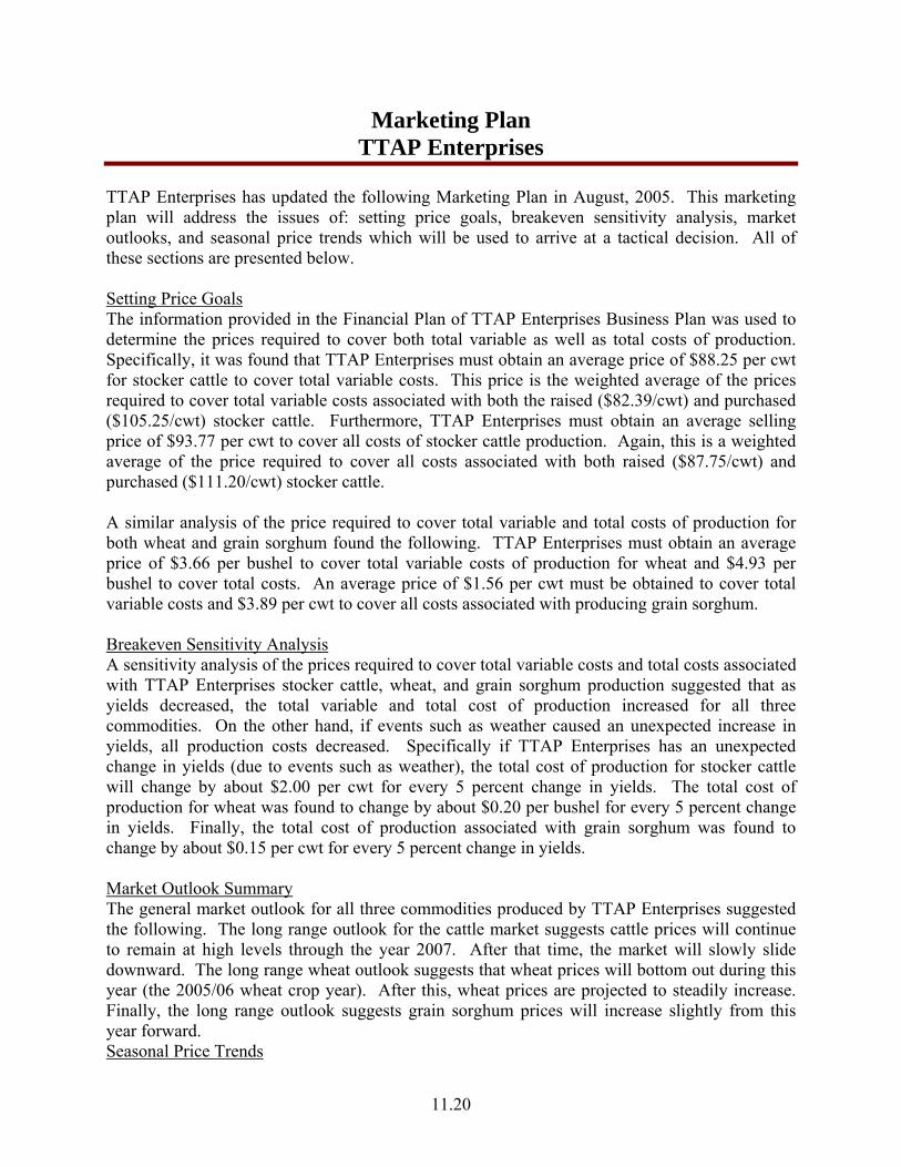
Marketing Plan TTAP Enterprises

TTAP Enterprises has updated the following Marketing Plan in August, 2005. This marketing plan will address the issues of: setting price goals, breakeven sensitivity analysis, market outlooks, and seasonal price trends which will be used to arrive at a tactical decision. All of these sections are presented below. Setting Price Goals The information provided in the Financial Plan of TTAP Enterprises Business Plan was used to determine the prices required to cover both total variable as well as total costs of production. Specifically, it was found that TTAP Enterprises must obtain an average price of $88.25 per cwt for stocker cattle to cover total variable costs. This price is the weighted average of the prices required to cover total variable costs associated with both the raised ($82.39/cwt) and purchased ($105.25/cwt) stocker cattle. Furthermore, TTAP Enterprises must obtain an average selling price of $93.77 per cwt to cover all costs of stocker cattle production. Again, this is a weighted average of the price required to cover all costs associated with both raised ($87.75/cwt) and purchased ($111.20/cwt) stocker cattle. A similar analysis of the price required to cover total variable and total costs of production for both wheat and grain sorghum found the following. TTAP Enterprises must obtain an average price of $3.66 per bushel to cover total variable costs of production for wheat and $4.93 per bushel to cover total costs. An average price of $1.56 per cwt must be obtained to cover total variable costs and $3.89 per cwt to cover all costs associated with producing grain sorghum. Breakeven Sensitivity Analysis A sensitivity analysis of the prices required to cover total variable costs and total costs associated with TTAP Enterprises stocker cattle, wheat, and grain sorghum production suggested that as yields decreased, the total variable and total cost of production increased for all three commodities. On the other hand, if events such as weather caused an unexpected increase in yields, all production costs decreased. Specifically if TTAP Enterprises has an unexpected change in yields (due to events such as weather), the total cost of production for stocker cattle will change by about $2.00 per cwt for every 5 percent change in yields. The total cost of production for wheat was found to change by about $0.20 per bushel for every 5 percent change in yields. Finally, the total cost of production associated with grain sorghum was found to change by about $0.15 per cwt for every 5 percent change in yields. Market Outlook Summary The general market outlook for all three commodities produced by TTAP Enterprises suggested the following. The long range outlook for the cattle market suggests cattle prices will continue to remain at high levels through the year 2007. After that time, the market will slowly slide downward. The long range wheat outlook suggests that wheat prices will bottom out during this year (the 2005/06 wheat crop year). After this, wheat prices are projected to steadily increase. Finally, the long range outlook suggests grain sorghum prices will increase slightly from this year forward. Seasonal Price Trends

11.21

An analysis of historical prices found that there does appear to be a seasonal price trend for cattle in Texas. Specifically, the price of all types of cattle appears to be higher in the late Winter/early Springs months (February, March, April) and lower in the Fall months (September, October, and November). The one exception is found in Fed Steer prices in Texas. The lowest prices are generally found in the Summer months (June, July, August, and September). Seasonal price trends were also found in wheat and corn (which is being used as a substitute for grain sorghum due to a lack of information). The seasonal trend for wheat is that the lowest price of the year is found in July. Prices then tend to slowly increase until about November. After November, prices slowly start to decline until July. As with wheat, the lowest price of the year for corn appears to be in July. After July, prices increase steadily until about April. Corn prices then fall quickly from this high in April to the low in July. Tactical Decisions Using the information provided above, the following tactical decisions were made regarding the marketing of TTAP Enterprise’s stocker cattle. Given that the general price level of cattle are in the top third of historical prices, the long term outlook for cattle is down, the short term market outlook is flat, seasonal price outlook is down, and the current local basis is in the middle third, TTAP Enterprises has decided to price 100 percent of its cattle that will be ready in May through forward contracts. This decision follows the a priori decision for this commodity. TTAP Enterprises has decided to follow the a priori decision regarding wheat under the conditions that are currently being observed. Specifically, the general price level is in the middle third, the long term outlook is up, the short term outlook is down, the seasonal price trend outlook is up, and current local basis is in the middle third. TTAP Enterprises would like to just sit and watch this market for a couple more months and see if prices will follow the seasonal trend. The tactical marketing decision regarding grain sorghum is to not do anything. Grain sorghum has always been a secondary crop for TTAP Enterprises and will remain that way. Given this information, TTAP Enterprises will harvest the crop and get the best local price available.

11.22

Case Study Strategic Marketing Plan

Worksheets

11.23

Strategic Marketing Plan Worksheet 1 Industry Profile – Beef

Source: http://www.ers.usda.gov/Briefing/ & http://www.ers.usda.gov/Briefing/Cattle/Trade.htm

Background With its abundant grasslands and large grain supply, the United States has developed a beef industry that is largely separate from its dairy sector. The United States has the largest fed-cattle industry in the world, and is the world's largest producer of beef, primarily high-quality, grain-fed beef for domestic and export use. The industry is roughly divided into two production sectors: cow-calf operations and cattle feeding. Cattle Cycle

The cattle cycle refers to increases and decreases in cattle herd size over time. The cattle cycle is usually 8-12 years in duration, the longest of all meat animals. The last cattle cycle lasted 12 years and the present cycle is in its 14th year, with 2 more years of decline likely. The cattle cycle is determined by the combined effects of cattle prices and the time needed to breed, birth, and raise cattle to market weight.

Given the dry conditions that have persisted since 1998, retention of enough heifers to turn the cycle is unlikely to begin until forage conditions improve and heifers are retained. The first real opportunity for meaningful change will come with heifers born in 2004. These heifers were born in late winter-early spring 2004 and would be weaned in the fall, bred in late spring-early summer 2005, and calve 9 months later. These additional heifers and calves could result in an expansion to be first reported in the January 1, 2007, cattle inventory report. The National Agricultural Statistics Service (NASS) provides information on cattle numbers in semi-annual inventory reports.

Cow-Calf Operations These operations are located throughout the United States, typically on land not suited or needed for crop production. Cow-calf operations are dependent upon range and pasture forage conditions, which are in turn dependent upon variations in the average level of rainfall and temperature for the area. Beef cows harvest forage from grasslands to maintain themselves and raise a calf with very little, if any, grain input. The cow is maintained on pasture year round, as is the calf until it is weaned. If additional forage is available at weaning, some calves may be retained for additional grazing and growth until the following spring when they are sold. The average beef cow herd is 40 head, but operations with 100 or more beef cows comprise 9 percent

11.24

of all beef operations and 51 percent of the beef cow inventory. Operations with 40 or fewer head are largely part of multi-enterprises, or are supplemental to off-farm employment. Cattle Feedlots Cattle feeding is concentrated in the Great Plains, but is also important in parts of the Corn Belt, Southwest, and Pacific Northwest. Cattle feedlots produce high-quality beef, grade Select or higher, by feeding grain and other concentrates for about 140 days. Depending on weight at placement, feeding conditions, and desired finish, the feeding period can be from 90 to as long as 300 days. Average gain is 2.5-4 pounds per day on about 6 pounds of dry-weight feed per pound of gain. While most of a calf's nutrient inputs until it is weaned are from grass, feedlot rations are generally 70 to 90 percent grain and protein concentrates. Feedlots with less than 1,000 head of capacity comprise the vast majority of U.S. feedlots but market a relatively small share of fed cattle. In contrast, lots with 1,000 head or more of capacity comprise less than 5 percent of total feedlots but market 80-90 percent of fed cattle. Feedlots with 32,000 head or more of capacity market around 40 percent of fed cattle. The industry continues to shift toward a small number of very large specialized feedlots, which are increasingly vertically integrated with the cow-calf and processing sectors to produce high-quality fed beef. NASS provides monthly Cattle on Feed reports.

U.S. Beef Trade

The United States, while the largest producer of beef in the world, is a net beef importer. Most beef produced and exported from the United States is grain-finished, high-quality choice cuts. Most beef that the United States imports is grass-fed beef, destined for processing, primarily as ground beef.

11.25

The largest export market for U.S. beef is Japan, which through 2000 imported at least twice as much U.S. beef as the second-largest U.S. export market. However, imports by Japan fell by about one-third late in 2001 when BSE was discovered in the Japanese cattle herd. Mexico is the second-largest market for U.S. beef, and continued growth is expected but at a slower pace than in the past. The third-largest export market for U.S. beef, and the fastest growing, has been South Korea. The Korean market became fully liberalized at the end of 2001 and rapid growth is expected to continue. Canada, in fourth place, has been gradually declining in importance for several years. The Canadian market is expected to grow slowly at best.

Over the past several years, the largest percentage of U.S. beef imports has come from Australia, with Canada a close second. The third-largest exporter of beef to the United States is New

11.26

Zealand. The United States also imports a significant portion of its cooked beef from Argentina and Brazil, but their combined share of the U.S. beef market is less than half that of the three largest exporters. The remainder of U.S. beef imports comes from Central America and Uruguay.

In May 2003, Canada reported the discovery of a case of BSE in one of its beef cows. Cattle and beef products from Canada were barred entry into the United States after the announcement. In August 2003, beef imports from Canada resumed but were restricted to boneless products from cattle under 30 months of age. As of early 2004, the trade situation continues to evolve as officials review the risks and revise trading rules accordingly.

The United States imports a significantly greater volume of cattle than it exports. The countries from which the United States imports cattle are also the same ones to which it exports cattle: Canada and Mexico. The geographical proximity of these countries and complementarity of their cattle and beef sectors explains why they are the United States' only significant cattle trading partners. Imports of Canadian cattle into the United States, however, have been banned since the May 2003 BSE announcement.

11.27

U.S. cattle exports to Canada and Mexico vary from year to year in the relative percentage exported to each country, although the absolute level of trade has been greater over the last several years. Historically, the United States exported primarily slaughter cattle to both countries. However, changes in Canada's policies have led to increased exports of feeder cattle.

In past years, cattle imports from Canada and Mexico have varied. The relative share of cattle imported from Mexico has tended to increase over the last several years. Imports from Mexico tend to be lighter cattle for finishing in U.S. feedlots, while those from Canada tended to be primarily for slaughter.

11.28

Strategic Marketing Plan Worksheet 1 (Continued) Industry Profile – Wheat

Source: USDA-ERS http://www.ers.usda.gov/Briefing/

Background

The United States is a major wheat-producing country, with output typically exceeded only by China, the European Union, and, sometimes, India. During the early 2000s, wheat ranked third among U.S. field crops in both planted acreage and gross farm receipts, behind corn and soybeans. Presently, almost half of the U.S. wheat crop is exported.

The U.S. wheat sector enters the 21st century facing many challenges, despite a strong domestic market for wheat products. U.S. wheat harvested area has dropped off 28 million acres, or nearly one-third from its peak in 1981, because of declining returns compared with other crops and alternative options under government programs. Despite rising global wheat trade, U.S. share of the world market has eroded in the past two decades.

U.S. Wheat Classes

Wheat is the principal food grain produced in the United States. Wheat varieties grown in the United States are classified as "winter wheat" or "spring wheat," depending on the season each is planted. Winter wheat production represents 70-80 percent of total U.S. production. Winter wheat varieties are sown in the fall and usually become established before going into dormancy when cold weather arrives. In the spring, plants resume growth and grow rapidly until summertime harvest. In the Northern Plains, where winters are harsh, spring wheat and durum wheat are planted in the spring and harvested in the late summer or fall of the same year.

The five major classes of U.S. wheat are hard red winter, hard red spring, soft red winter, white, and durum. Each class has a somewhat different end use and production tends to be region-specific.

• Hard red winter (HRW) wheat accounts for about 40 percent of total production and is grown primarily in the Great Plains (Texas north through Montana). HRW is principally used to make bread flour.

• Hard red spring (HRS) wheat accounts for about 25 percent of production and is grown primarily in the Northern Plains (North Dakota, Montana, Minnesota, and South Dakota). HRS wheat is valued for high protein levels, which make it suitable for specialty breads and blending with lower protein wheat.

11.29

• Soft red winter (SRW) wheat, accounting for 15-20 percent of total production, is grown primarily in States along the Mississippi River and in the Eastern States. Flour produced from milling SRW is used in the United States for cakes, cookies, and crackers.

• White wheat, accounting for 10-15 percent of total production, is grown in Washington, Oregon, Idaho, Michigan, and New York, and its flour is used for noodle products, crackers, cereals, and white-crusted breads.

• Durum wheat, accounting for 3-5 percent of total production, is grown primarily in North Dakota and Montana and is used in the production of pasta.

Wheat milling byproducts—such as bran (outer seed coat of a wheat kernel), shorts (more inward layers of the seed coat that contain some starchy or floury components), and middlings (an intermediate fraction that consists of a combination of bran and shorts)—are used by feed manufacturers in the production of animal feeds.

U.S. Wheat Supply

Wheat area has dropped from its early 1980s highs, due mostly to declining returns relative to other crops and alternative options under government programs. Authorization of the Conservation Reserve Program (CRP) in the 1985 Farm Act, followed by planting flexibility provisions in the 1990 Farm Act, provided wheat farmers with other options for use of their acreage. Under the 1990 Act, farmers participating in commodity programs could plant up to 25 percent of their base wheat acreage to crops other than wheat without losing base acreage. Farmers thus had an incentive to grow crops promising higher returns or to earn rental payments from idling land under the CRP.

Planting flexibility facilitated expansion of soybeans, corn, and other crops in traditional wheat areas. The 1996 Farm Act completed the market orientation of crop planting by eliminating the requirement to maintain base acreage of program crops in order to qualify for government payments.

The role and nature of government assistance to the farm sector is under intense debate because of variable commodity prices. While low profitability of wheat has encouraged some farmers to switch to other crops, many farmers cannot easily switch from wheat. In addition to watching market prices to decide what and how much to plant, farmers are strongly influenced by loan deficiency payments. Farmers in the Eastern United States, with higher rainfall, have more profitable alternatives to wheat than in other wheat-growing regions. Profitable alternative crop choices to dryland wheat in the Plains regions, while more limited, do exist.

Loss of wheat acreage to row crops on the Plains reflects strong genetic improvements in corn and soybeans, producing varieties that could be planted farther west and north in the region, areas with drier conditions or shorter growing seasons. The pace of genetic improvement has been slower for wheat than for some other field crops, making wheat less competitive for

11.30

cropland. Genetic improvement is slower because of genetic complexity and because of lower potential returns to commercial seed companies, which discourage investment in research. In the corn sector, for example, where hybrids are used, farmers generally buy seed from dealers every year. However, many wheat farmers, particularly in the Plains States, use saved seed instead of buying from dealers every year.

U.S. Wheat Use

U.S. consumer demand for food products made from wheat flour is relatively unaffected by changes in wheat prices or disposable income. However, demand is closely tied to population, tastes, and preferences.

The strength of the domestic market for wheat has developed out of the historic turnaround that occurred in the 1970s in U.S. per capita wheat consumption. For nearly 100 years, per capita wheat consumption declined in the United States, as hard physical labor became less common and diets diversified. Wheat consumption dropped from over 225 pounds per person in 1879 to 180 pounds in 1925 before bottoming out at 110 pounds in 1972. By 1997, consumption had rebounded to 147 pounds per capita. The rise in consumption benefited the U.S. wheat processing industry, which has operated near full capacity over the last 25 years, while expanding and modernizing.

However, the growth in per capita consumption appears to have ended. Since 1997, per capita consumption has fluctuated slightly from year to year, dropping 10 pounds during 2001 and 2002, and leveling off in 2003. The sharp drop may reflect, in part, the increasing numbers of weight-conscious consumers following diets that include fewer carbohydrates. Another force reducing flour usage (and thus, wheat consumption) is the expanding production of extended shelf life bread. The outcome for U.S. bakers is a reduction in "stales" (bread that does not sell and is taken back by the baker) from as high as 15 percent of sales to less than 8 percent. Reducing stales directly reduces the quantity of flour required to supply the same level of consumer demand. The downturn in per capita consumption has created some financial distress because of milling and baking overcapacity and has raised concerns about prospective consumer tastes and preferences.

Almost half of the U.S. wheat crop is exported. The importance of exports varies by class of wheat. The white and HRS classes rely more than others on sales into export markets:

• White wheat, two-thirds of the crop exported • HRS, half of the crop exported • SRW and durum, about one-third of each exported • HRW, slightly over one-third exported

In the 1990s and early 2000s, world wheat consumption continued to expand in response to rising population and incomes, but the volume of world trade gained only slightly. Distribution of global wheat trade broadened as small purchases by a larger number of importing countries—

11.31

in Southeast Asia, North Africa, and the Middle East—have together become more important than the very large purchases in the past by the former Soviet Union and China.

The United States has lost share in global wheat trade over the years, and export competition will not abate in the foreseeable future. Agricultural policy reforms in the European Union's (EU) Agenda 2000 are expected to promote wheat production in EU countries over other crops. Traditional exporters (Argentina, Australia, and Canada) are expected to continue to be very competitive. Other suppliers, such as Eastern Europe and parts of the former Soviet Union, also may provide increased export competition if their infrastructure improves and if they upgrade the quality of wheat output while holding down costs.

U.S. Wheat Prospects

Challenges for the U.S. wheat sector will not abate in the foreseeable future. Other crops will be included in farmers' production decisions under current farm legislation. Although wheat products have proven to be competitive with other foodstuffs in the domestic market in recent years, foreign competition will continue to pressure U.S. wheat producers.

Research to develop new varieties and new growing methods may improve market competitiveness and increase the cost efficiency of wheat production. Improved varieties of U.S. hard white wheat, for example, have been developed using traditional genetic breeding methods, and some breeders and industry analysts believe these hard whites may open new market prospects to U.S. producers in Asia and the Middle East, where Australian white wheat now dominates. Development of genetically modified, herbicide-tolerant wheat varieties promises significant benefits to spring wheat growers, but may also introduce some uncertainty in marketing.

11.32

Strategic Marketing Plan Worksheet 1 (Continued) Industry Profile - Grain Sorghum http://www.ers.usda.gov/Briefing/

Background Grain sorghum is the third most important cereal crop grown in the United States and the fifth most important cereal crop grown in the world. The United States is currently positioned as the number one producer and exporter of sorghum on the world market. The United States' share of world trade in sorghum has not dropped below 70 percent in the last decade. World trade in sorghum is dominated by U.S. exports to Mexico. Other importing countries and regions include Japan, Israel, Eritrea, South Africa and the European Union. Grain sorghum is utilized in food and industries around the world, as well as being a staple feed ingredient in the U.S. Worldwide, more than 50 % of sorghum is grown directly for human consumption. Other uses for grain sorghum include the production of wallboard for the housing industry and ethanol. Sorghum Supply Historically, Kansas and Texas have been the largest grain sorghum producing states in the United States. Between 1982 and 2002 the two states combined have produced, on average, 62.4 percent of the sorghum in the United States. U.S. sorghum production in 2003 was 411 million bushels. Of that, Kansas raised 130.5 million bushels in 2003 and Texas grew nearly 154 million bushels. Sorghum Demand Sorghum has a variety of uses including food for human consumption, feed grain for livestock, and industrial applications such as ethanol production. The area planted to sorghum worldwide has increased by 66 percent over the past 50 years while yield has increased by 244 percent. Around half of sorghum produced is fed to livestock and half is consumed by humans and used in other applications. Currently most human consumption of sorghum occurs in low-income countries whereas high-income countries typically use sorghum as a component in livestock feed. Sorghum is a versatile plant as it can tolerate drought, soil toxicities, a wide range of temperatures, and high altitudes. As 25 percent of the population is expected to undergo severe water shortage by 2025, the crop’s adaptability suggests that it may soon play a larger role in supplying the world with grain. While globally, about 50 percent of sorghum is consumed by humans, in the United States over 90 percent of the sorghum consumed is used as a component in livestock feed. Corn is the main

11.33

substitute of sorghum for use in feed. The starch and protein in sorghum are more difficult for animals to digest than those in corn. This gives corn a distinct advantage for feed usage. However, research is being conducted to develop processing methods that allow animals to digest sorghum more readily. Processing breaks the seed coat, reduces particle size, and increases surface area. Some methods of processing make the end-use value of sorghum comparable to that of corn because more starch and protein are able to be digested in sorghum. While many new sorghum food products are currently being developed, the grain’s food use has been limited thus far. These limitations are mainly due to two characteristics of the plant. First, phenolic acid and tannins cause flour made from sorghum to have a bitter flavor. Second, the lack of gluten restricts sorghum’s usefulness in the food industry. Recently a food grade sorghum has been developed that does not contain phenolic acid or tannins and, hence, its flour does not have a bitter taste. These varieties are being used in snack food applications in the United States and Japan and can also be used to replace wheat flour in some baked products. The lack of gluten may be an advantage in a niche market targeting people who are gluten intolerant. Besides feed and food applications, sorghum is utilized in several other products. Archer Daniels Midland produces wallboard for the housing industry using sorghum. Due to its lack of conductivity, sorghum is becoming a popular material for biodegradable packaging materials. In industrial applications sorghum is increasingly being utilized in ethanol production. Currently around 10 percent of the U.S. sorghum crop is consumed by ethanol production. Ethanol can be produced from various crops including corn, wheat, and grain sorghum. Corn is used most often in ethanol production and sorghum is second. Eight plants in the United States use sorghum to produce ethanol. Five of these plants are located in Kansas. Since Kansas is continuously a top producer of sorghum, this crop is a reliable source for ethanol production. Kansas produces between 65 and 70 million gallons of fuel ethanol each year. This production generates a demand for about 26 million bushels of grain. Prices U.S. sorghum production averaged $4.40/cwt. in 2003. Corn averaged $2.45/bushel in 2003. Since the crops are close substitutes and have similar growing seasons, it is expected that their prices would move together. The average price difference between 1982 and 2002 was 19 cents per bushel premium on corn.

11.34



Commodity

Months Away From

Market Month




Prices


Marketing Decision

Stocker Cattle 6 Months

Top Third

Price 75% of expected production to ensure at least 20% profit & watch market.

Stocker Cattle 6 Months Top Third Price 50% of expected

production to ensure at least 20% profit & watch market

Stocker Cattle 6 Months Top Third

Price 100% of expected production


Middle Third

Hold tight & watch market

Stocker Cattle 6 Months Middle Third



Price 30% of expected production to ensure at least

break-even


Lower Third

Hold tight, watch market & hope for the best.

Stocker Cattle 6 Months Lower Third



Hope for a turnaround

11.35

Strategic Marketing Plan Worksheet 2 - Assessing Risk Tolerance A Priori Decision Tree – 6 Months Away From Marketing Month


Commodity

Months Away From

Market Month




Prices


Marketing Decision

Wheat 6 Months

Top Third

Price 75% of expected production to ensure at least 20% profit & watch market.

Wheat 6 Months Top Third

Price 50% of expected production to ensure at least 20% profit & watch market



Wheat 6 Months

Middle Third


Wheat 6 Months Middle Third

Price 33% of expected production & watch market



break-even

Wheat 6 Months

Lower Third


Wheat 6 Months Lower Third

Hold tight, watch market & hope for best


Watch market & hope for a turnaround

11.36



Commodity

Months Away From

Market Month




Prices


Marketing Decision

Grain Sorghum 6 Months

Top Third

N/A

Grain Sorghum 6 Months Top Third

N/A


N/A


Middle Third

N/A

Grain Sorghum 6 Months Middle Third

N/A


N/A


Lower Third

N/A

Grain Sorghum 6 Months Lower Third

N/A


N/A

11.37



Commodity

Months Away From

Market Month




Prices


Marketing Decision


Top Third

Hold tight but watch market

Stocker Cattle 3 Months Top Third Price 75% of expected

production to ensure at least 20% profit & watch market

Stocker Cattle 3 Months Top Third



Middle Third






break-even.


Lower Third





Talk to banker

11.38



Commodity

Months Away From

Market Month




Prices


Marketing Decision

Wheat 3 Months

Top Third

Hold Tight But Watch Market

Wheat 3 Months Top Third Price 100% of expected

production to ensure at least 20% profit & watch market.



Wheat 3 Months

Middle Third






break-even.

Wheat 3 Months

Lower Third





Hope for a turnaround

11.39



Commodity

Months Away From

Market Month




Prices


Marketing Decision


Top Third

N/A


N/A


N/A


Middle Third

N/A


N/A


N/A


Lower Third

N/A


N/A


N/A

11.40

Strategic Marketing Plan Worksheet 4 Setting Price Goals

Commodity Expected Yearly Production


Total per Unit Cost of Production

Stocker Cattle1

(Raised) (Purchased)

2,921.40 cwt (2,171.40 cwt) (750.00 cwt)

$88.25/cwt ($82.39/ cwt) ($105.25/cwt)

$93.77/cwt ($87.75/ cwt) ($111.20/cwt)

Wheat 15,000 bu. $3.66/bu. $4.93/bu.

Grain Sorghum 4,200 cwt. $1.56/cwt. $3.89/cwt.

1.Variable costs were determined by the following formula: (Direct Variable Stocker Cost) + [(Direct Wheat Variable Cost/Total Wheat Cost)*(Grazing Cost)]

11.41

Strategic Marketing Plan Worksheet 5 Breakeven Sensitivity Analysis

Commodity Yield Sensitivity

Expected Yearly

Production


Total per Unit Cost of

Production

20% Yield Decrease 2,337.12 cwt $99.69/cwt $106.59/cwt 15% Yield Decrease 2,483.19 cwt $96.23/cwt $102.72/cwt 10% Yield Decrease 2,629.26 cwt $93.21/cwt $99.35/cwt 5% Yield Decrease 2,775.33 cwt $90.57/cwt $96.38/cwt

Average Yields 2,921.40 cwt $88.25/cwt $93.77/cwt 5% Yield Increase 3,067.47 cwt $86.15/cwt $91.41/cwt 10% Yield Increase 3,213.54 cwt $84.29/cwt $89.31/cwt 15% Yield Increase 3,359.61 cwt $82.64/cwt $87.44/cwt

Stocker Cattle

20% Yield Increase 3,505.68 cwt $81.18/cwt $85.78/cwt

20% Yield Decrease 12,000 bu. $4.13/bu. $5.72/bu. 15% Yield Decrease 12,750 bu. $3.99/bu. $5.49/bu. 10% Yield Decrease 13,500 bu. $3.87/bu. $5.28/bu. 5% Yield Decrease 14,250 bu. $3.76/bu. $5.09/bu.

Average Yields 15,000 bu. $3.66/bu. $4.93/bu. 5% Yield Increase 15,750 bu. $3.57/bu. $4.78/bu. 10% Yield Increase 16,500 bu. $3.50/bu. $4.65/bu. 15% Yield Increase 17,250 bu. $3.43/bu. $4.53/bu.

Wheat

20% Yield Increase 18,000 bu. $3.37/bu. $4.42/bu.

20% Yield Decrease 3,360 cwt $1.76/cwt $4.67/cwt 15% Yield Decrease 3,570 cwt $1.70/cwt $4.44/cwt 10% Yield Decrease 3,780 cwt $1.65/cwt $4.24/cwt 5% Yield Decrease 3,990 cwt $1.60/cwt $4.05/cwt

Average Yields 4,200 cwt $1.56/cwt $3.89/cwt 5% Yield Increase 4,410 cwt $1.52/cwt $3.74/cwt 10% Yield Increase 4,620 cwt $1.49/cwt $3.61/cwt 15% Yield Increase 4,830 cwt $1.46/cwt $3.49/cwt

Grain Sorghum

20% Yield Increase 5,040 cwt $1.43/cwt $3.38/cwt

11.42

Strategic Marketing Plan Worksheet 6 Market Outlook & Expectations – Beef Cattle

Source: http://www.ers.usda.gov/Briefing/Cattle/Outlook.htm & http://www.ers.usda.gov/Briefing/Baseline/livstk.htm

Beef Prices Gain Relative to Competing Meats Cattle and beef prices strengthened as the cattle inventory reached the low point in the cattle cycle, and beef production declined. Although the cattle sector has been reducing cow slaughter and retaining heifers for the expansion phase of the new cattle cycle, beef production will not begin to expand to a large degree until mid-2007. Cow-calf operators, after suffering through drought in many areas from 1998 through 2004, are now able to expand due to improved forage conditions and continued strong prices for their calves. However, feedlot and stocker operator returns have been very erratic due to the record stocker/feeder cattle prices and difficulty in passing the higher calf prices on in the marketing system against relatively lower priced competing meats. Herd Expansion Continues First-half female slaughter continues to decline fairly sharply. Total cow slaughter was down 7 percent, with beef cow slaughter down 8 percent and dairy cow slaughter down 5 percent. Similarly heifer slaughter is down 7 percent compared with first-half 2004. The mid-year Cattle report to be released July 22, will give a firmer indication of just how strong a herd expansion is under way. In addition the report will provide the first estimate on this year’s calf crop, expected to show the first year-to-year gain since 1994. The number of heifers being retained will provide a first cut on the 2006 calf crop and rate of production expansion beginning in mid-2007 when the 2006 calf crop begins to be marketed from feedlots. Spring Choice Beef Prices Set Record In 2001 and 2002 retail prices for Choice beef averaged $3.35 a pound, while pork and broilers averaged $2.68 and $1.60 a pound, respectively. In 2004 beef prices had risen to $4.04 a pound, while pork and poultry averaged $2.79 and $1.74 a pound. In the second quarter of this year beef prices averaged a record $4.23 a pound. Pork prices averaged $2.87 a pound and broilers averaged $1.73 a pound. The beef/pork price ratio in 2001-2002 was 1.25, while in the second quarter it widened to 1.48. The beef/broiler price ratio has widened from 2.09 in 2001-2002 to 2.45. The near-record beef prices provide evidence of the present strong consumer demand for beef, but it also raises concern about the relatively high prices today against competing meats. In addition, higher petroleum, energy, and interest costs are taking a bigger bite out of consumers’ discretionary incomes. Second-quarter retail prices for Choice beef set a record this spring at $4.23 a pound, up nearly 2 percent from the former record set in fourth-quarter 2003 at $4.17 a pound and up over 3 percent from a year earlier. Beef prices have likely set the highs for the turning point of this cattle cycle

11.43

as beef supplies increase seasonally in the second half of the year and as cattle under 30 months of age enter the market from Canada. Pork and broiler production are expected to rise 3 to 4 percent over year-earlier levels in the second half of 2005, putting additional pressure on the relatively more expensive beef. After averaging $4.26 a pound in April and May, Choice retail beef prices declined to $4.18 a pound in June, about unchanged from June 2004. Cattle Prices Also at Record Levels Cattle prices continued on a record setting path in the first half of this year with fed cattle prices averaging in the upper $80s per cwt and Utility cows averaging in the upper $50s, both the result of tight beef supplies and continued strong beef demand. First-half beef production was down over 1 percent from a year earlier and down nearly 10 percent from 2003 when the May 20 ban on Canadian beef /cattle due to Bovine Spongiform Encephalopathy (BSE) was implemented. The ban on Canadian boneless beef from cattle under 30 months of age was lifted in August 2003. First-half prices for yearling feeder cattle were sharply above the year-earlier levels as tight supplies resulted in strong competition between cattle feeders and stocker operators. Producers in most of the country are experiencing the best grazing conditions in years. Although cattle feeders were in the black this spring, breakeven prices by mid-summer are moving toward the mid- to upper-$80s per cwt, reflecting record feeder cattle prices and modestly higher grain prices. Fed cattle prices are expected to average in the lower $80s this summer, putting margins in the red and taking some of the bloom off feeder cattle prices. Expected marginally larger feeder cattle supplies from this year’s calf crop will also take some of the premium off stocker/feeder cattle prices. U.S. Livestock Baseline Projections, 2005-2014

Livestock sector projections over the baseline period reflect strong domestic demand for meat. Beef and poultry exports rise from the reduced levels of 2004 that reflected concerns with bovine spongiform encephalopathy (BSE) and Avian influenza, respectively. The baseline assumes a gradual rebuilding of U.S. beef exports to Japan, reflecting the October 2004 U.S.-Japan beef trade framework agreement that will permit the resumption of beef trade between the two countries. While overall meat exports benefit from stronger foreign economic growth in the baseline, U.S. beef exports do not return to levels attained prior to the discovery of a U.S. BSE case in December 2003.

Moderate returns to red meat production lead to only small gains in beef and pork production in the second half of the projections. Larger gains in poultry output result in poultry becoming a larger proportion of total U.S. meat consumption as per capita beef consumption declines and per capita pork consumption levels off.

11.44

11.45

Baseline Trade Assumptions for Cattle and Beef

Due to uncertainties regarding the length of bans on trade in ruminants and ruminant products following the discovery of cases of BSE in the United States and Canada, the baseline projections for meats are based on a number of key assumptions related this issue.

Canadian Beef Exports

Canadian beef exports have rebounded from the lows of 2003 following the Canadian BSE case in May of that year, but do not fully recover to 2002 levels in the baseline projections.

U.S. Beef Exports

The baseline assumes a resumption of U.S. beef exports to Japan beginning in 2006, facilitated by the October 2004 U.S.-Japan beef trade framework agreement that will permit the reopening of beef trade between the two countries. Japanese imports of U.S. beef are assumed to grow slowly in the projections as the U.S. industry adopts the requirements under the framework agreement. The baseline also assumes a gradual recovery in U.S. beef exports to South Korea.

Canadian Cattle Exports to the United States

The resumption of imports from Canada of slaughter cattle under 30 months of age and feeder cattle is also assumed to begin in 2006 in the baseline. However, after the projections were prepared, a minimal risk rule was published which specifies USDA's regulations on meat and ruminant imports from regions with effective BSE prevention and detection measures. The rule becomes effective on March 7, 2005, and Canada will be the first country to be recognized as a minimal-risk region.

When the minimal risk rule becomes effective, imports of under-30-month-old steers and heifers from Canada for immediate slaughter and imports of Canadian feeder cattle that will enter U.S. feedlots are expected to lead to increased levels of cattle slaughter and beef production in the United States in 2005 and 2006, with somewhat lower cattle and beef prices. Larger beef supplies are also expected to pressure prices for other livestock and other meats.

11.46

U.S. beef production increases from the sharp declines of 2003 and 2004. Despite the loss of export markets following the case of BSE in late 2003, strong domestic demand for beef has resulted in favorable producer returns which, together with favorable forage and feed grain supplies, begins the process of retention of cows and heifers for future expansion. Cattle herds are expected to increase somewhat from cyclical lows near 95 million head in 2005 and 2006. Rising slaughter weights augment gradual herd expansion over the remainder of the projections. Pork production grows slowly as the coordinated/integrated industrial structure dampens the U.S. hog cycle. Poultry production continues to rise, but at a lower rate than during the 1990s due to the maturity of domestic demand and slower export growth.

The trend toward larger livestock systems continues throughout the baseline period. Efficiency gains allow production to expand while real prices generally decline.

• Strong demand for consistent, higher quality beef continues in the domestic hotel and restaurant market and increasingly in the retail market. Additionally, the rebuilding of beef export markets is primarily for high-quality beef. Increasing movement toward transparent animal identification in international trade will strengthen quality assurance.

• Increased efficiency of the U.S. hog breeding herd is reflected in a shift to larger, more efficient operations and in the decline of smaller, less efficient operations. For the baseline, the increase in efficiency slows somewhat since larger, more efficient operations already account for a large share of the U.S. pig crop.

• Production coordination and market integration between the United States and Canada continues to increase in the hog sector. Canada is the major supplier of live hog imports to the United States. Feeder pigs produced in Canada are finished and processed in the United States, where feed grain prices remain favorable and processing costs are lower. Large wholesale and retail buyers source pork cuts where prices are attractive, with demand accommodated by trade between the two countries.

11.47

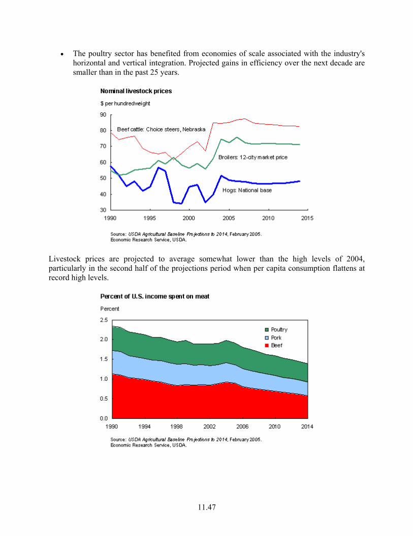
• The poultry sector has benefited from economies of scale associated with the industry's horizontal and vertical integration. Projected gains in efficiency over the next decade are smaller than in the past 25 years.

Livestock prices are projected to average somewhat lower than the high levels of 2004, particularly in the second half of the projections period when per capita consumption flattens at record high levels.

11.48

U.S. consumers buy more meat, but spend a smaller proportion of disposable income for these purchases, continuing a long-term trend. Over the next 10 years, consumer meat expenditures decline from about 2 percent to 1.4 percent of disposable income.

• Poultry expenditures continue to increase as a share of consumer spending on meats.

Higher levels of total per capita meat consumption are projected over the next decade, largely reflecting continued increases in poultry consumption. On a retail weight basis, per capita consumption rises to about 234 pounds from the 2004 level of 223 pounds.

• Per capita consumption of beef remains at relatively high levels through the baseline in part because beef exports, although growing, do not return to 2003 levels in the projections.

• Pork consumption remains stable at 52-53 pounds per person throughout the projections.

• Per capita consumption of relatively lower priced poultry increases throughout the baseline, allowing poultry to gain a larger share of total meat consumption and meat expenditures.

11.49

U.S. meat exports rise throughout the baseline period from the reduced levels in 2004 that reflected disease-related loss of markets, especially for beef and broilers. Improved global economic growth and rising demand for meats contribute to the gains in U.S. exports. The gradual recovery in beef exports to markets such as Japan and South Korea is also critical to the projections. The baseline assumes that Brazil and Argentina will not be recognized as free of foot-and-mouth disease (FMD) by key importing countries, such as Japan.

Beef

• U.S. beef exports primarily reflect demand for high-quality fed beef, with most U.S. beef exports typically going to markets in Pacific Rim nations. With the loss of those markets following the BSE case in the United States in late-December 2003, U.S. beef exports were sharply lower in 2004. However, U.S. beef exports are projected to rise slowly in the baseline as the October 2004 beef trade framework agreement between the United States and Japan facilitates the resumption of beef trade between the two countries. A gradual recovery in U.S. beef exports to South Korea is also assumed.

• U.S. imports of processing beef from Australia and New Zealand decline in the baseline as more, lower quality processing beef comes from domestic sources with the rebuilding of the cattle herd. The United States is a net beef importer on a volume basis through the projections as the recovery of high-quality fed beef exports does not reach prior levels.

Pork

• U.S. pork exports benefit somewhat from reduced beef exports as import demand shifts among competing meats. Pacific Rim nations and Mexico remain key markets for long-term growth of U.S. pork exports. Canada continues to be a strong competitor in these markets. Brazil also is a major pork exporter. However, without nationwide FMD-free

11.50

status, Brazil focuses its pork exports on Russia, Argentina, and Asian markets other than Japan and South Korea.

• While increased efficiency in pork production helps limit production costs, longer term gains in U.S. pork exports will be determined by costs of production and environmental regulations relative to competitors. Such costs tend to be lower in countries with growing pork industries, such as Brazil and Mexico.

Poultry

• U.S. broiler export growth is expected to slow from the rate of the 1990s. U.S. producers will face strong competition from other major broiler exporting countries, particularly Brazil.

• Major U.S. export markets include Asia, Russia, and Mexico. Gains in these markets reflect strong economic growth and rising consumer demand.

The sharp decline in beef exports in 2004 lowered the overall meat export share of the total value of domestically produced meat from about 11 percent in 2003 to under 8 percent, based on a measure that weights exports of beef, pork, and chicken by farm-level prices. While U.S. meat exports grow in importance in the projections, the domestic market remains the dominant source of demand and exports only recover to 10 percent of the production value.

11.51

Table 1. USDA-ERS Projected U.S. Beef Cattle Supply and Demand (March 14, 2005) Item Units 2005 2006 2007 2008 2009 2010 2011 2012 2013 2014 Beginning stocks Mil. lbs. 625 575 575 575 575 575 575 575 575 575 Commercial production Mil. lbs. 24,775 24,808 25,213 26,034 26,458 26,884 27,115 27,416 27,692 27,941 % change from previous year 1.1 0.1 1.6 3.3 1.6 1.6 0.9 1.1 1.0 0.9 Farm production Mil. lbs. 101 101 101 101 101 101 101 101 101 101 Total production Mil. lbs. 24,876 24,909 25,314 26,135 26,559 26,985 27,216 27,517 27,793 28,042 Imports Mil. lbs. 3,660 3,682 3,671 3,582 3,472 3,325 3,250 3,200 3,150 3,100 Total supply Mil. lbs. 29,161 29,166 29,560 30,292 30,606 30,885 31,041 31,292 31,518 31,717 Exports Mil. lbs. 620 682 750 825 908 1,044 1,200 1,381 1,588 1,826 Ending stocks Mil. lbs. 575 575 575 575 575 575 575 575 575 575 Total consumption Mil. lbs. 27,966 27,909 28,235 28,892 29,123 29,266 29,266 29,336 29,355 29,316 Per capita, carcass wgt Pounds 94.3 93.2 93.4 94.7 94.6 94.2 93.3 92.7 92.0 91.1 Per capita, retail wgt Pounds 66.0 65.2 65.4 66.3 66.2 65.9 65.3 64.9 64.4 63.7 Prices: Beef cattle, farm $/cwt 83.91 85.63 86.37 83.54 82.86 82.69 82.30 81.64 81.53 81.35 Calves, farm $/cwt 111.89 110.49 109.89 107.50 104.44 105.38 103.54 101.64 100.76 99.74 Retail: Beef & veal 1982-84=100 197.0 186.6 187.5 185.4 187.0 189.8 192.7 194.9 196.8 198.7 Retail: Other meats 1982-84=100 176.1 178.2 180.2 182.0 184.3 186.8 189.3 192.0 194.9 197.9 ERS retail beef $/lb. 4.10 3.88 3.90 3.86 3.89 3.95 4.01 4.06 4.10 4.14 Costs and returns, cow-calf enterprise: Variable expenses $/cow 221.52 224.26 227.62 232.88 238.75 243.44 247.46 250.51 253.86 257.29 Fixed expenses $/cow 125.71 131.06 136.39 140.95 143.78 146.20 148.53 150.81 153.12 155.71 Total cash expenses $/cow 347.23 355.32 364.01 373.83 382.53 389.64 395.99 401.32 406.97 413.00 Returns above cash costs $/cow 125.82 120.03 115.86 102.44 88.27 92.42 85.76 79.52 77.17 73.76 Cattle inventory 1000 head 94,732 94,711 95,842 96,490 97,171 97,646 98,170 98,671 98,901 98,776 Beef cow inventory 1000 head 32,592 32,402 32,804 33,232 33,633 33,927 34,066 34,241 34,322 34,335 Total cow inventory 1000 head 41,550 41,310 41,677 42,041 42,366 42,585 42,650 42,765 42,786 42,740

Source: http://www.ers.usda.gov/publications/oce051/oce20051d.pdf

11.52

Strategic Marketing Plan Worksheet 6 (Continued) Market Outlook & Expectations – Wheat

Source: http://www.ers.usda.gov/Briefing/Wheat/2005baseline.htm

Supply

Several long-term factors are important for determining the size of the U.S. wheat crop during 2005-14.

U.S. wheat planted area trending downward. Planted wheat area in the United States has trended down since its peak of 88 million acres in 1981, in part because of lower returns relative to other crops. Increased planting flexibility under the 1996 Farm Act facilitated expansion of soybeans and corn into traditional wheat areas, especially the Plains States. In addition, more wheat land was planted to minor oilseeds, such as canola. Finally, USDA's Conservation Reserve Program (CRP) removed 8 to 10 million of acres of land from production that had traditionally been planted to wheat. About one-fourth of CRP acres in the baseline is land that has historically been planted to wheat.

Rotations are changing. Changes in rotations, particularly in the dryland areas of the Great Plains, have also contributed to the decline in wheat acres. For example, in Kansas, a typical wheat-fallow rotation has been replaced most commonly by a rotation of wheat-grain sorghum-fallow, so that wheat is planted 1 year out of 3 years instead of 1 out of 2. Other crops, such as soybeans and corn, are also used in rotations. Studies from Kansas State University indicate that

11.53

multicrop rotations produce markedly higher net returns than a wheat-fallow rotation, primarily because of the inclusion of higher value, but riskier crops in the rotation mix.

Wheat disease also a factor. Concerns about wheat disease problems in the Northern Plains, particularly scab (head blight) in North Dakota and Minnesota (caused by the fungus Fusarium graminearum), influenced planting decisions in the 1990s and will do so in the future. The increased incidence may stem in part from switches to corn plantings and minimum tillage in traditional wheat areas in the Northern Plains. Both activities provide hosts for disease organisms.

Wheat's genetic improvement lags competing crops. Loss of wheat acreage to row crops in the Great Plains reflects genetic improvements in corn and soybeans, producing varieties that can be planted farther west and north in the region, areas with drier conditions or shorter growing seasons. The pace of genetic improvement has been slower for wheat than for some other field crops, resulting in little growth in wheat yields, which makes wheat a less attractive option for farmers. Genetic improvement for wheat is slower because of genetic complexity and because of lower potential returns to commercial seed companies, factors which discourage investment in research. In the corn sector, for example, where hybrids are used, farmers buy seed from dealers every year. However, many wheat farmers, particularly in the Plains States, plant seed saved from the previous harvest instead of buying from dealers.

Demand

Several factors underlie the long-term developments that will determine the domestic and foreign demand for U.S. wheat during 2005-14.

11.54

U.S. per capita food use appears to have peaked. Until recently, U.S. wheat producers could count on rising per capita food use of wheat flour to expand domestic demand for their crop. The strength of this domestic market developed out of the historic turnaround in U.S. per capita wheat consumption in the 1970s. U.S. per capita wheat consumption declined for nearly 100 years as caloric requirements decreased, because physical labor became less common and diets diversified. Wheat consumption dropped from over 225 pounds per person in 1879 to a low of 110 pounds in 1972.

Between 1973 and 1997, the growth in per capita consumption reflected the boom in away-from-home eating, the desire of consumers for greater variety and more convenience in food products, promotion of wheat flour and pasta products by industry organizations, and wider recognition of health benefits stemming from eating high-fiber, grain-based foods. By 1997, consumption had rebounded to 147 pounds per capita.

Since 1997, growth in per capita food use appears to have ended. Notably, per capita flour consumption has dropped sharply to 133 pounds in 2004. These changes may reflect, in part, the increasing numbers of health- and weight-conscious people following diets that include fewer carbohydrates.

Bread preservation is improving. Another force reducing flour usage is the expanding production of extended shelf life (ESL) bread. New ESL technologies can double or even triple the shelf life of a fresh loaf, from several days to 10 or more. The outcome for U.S. bakers is a reduction in "stales" (meaning bread that does not sell and is taken back by the baker) from as high as 15 percent of sales to less than 8 percent. Reducing stales directly reduces the quantity of flour required to produce enough bread to meet the same level of consumer demand.

11.55

Exports from Black Sea area have been increasing. Russia and Ukraine have emerged as significant exporters of wheat in recent years. In the 1992/93 crop year (July-June), the two countries exported 33 and 4 million bushels of wheat, respectively. By 2002/03, exports had reached 464 and 243 million bushels, respectively. Russia's 2002/03 exports reflected nearly ideal weather and prevailing high prices. Production in Russia and Ukraine is unstable year to year because of variable weather conditions.

The Black Sea area is emerging from the economic adjustments experienced during its transition to independence following the breakup of the Soviet Union. One reason Russia has been able to export so much wheat is that its livestock sector has been reduced sharply, cutting the domestic demand for wheat feeding. In addition, investments in infrastructure were made, especially port facilities, by countries in the Black Sea region to enhance their future trade competitiveness.

Baseline projections for U.S. wheat supply and use

Highlighted here are key findings for U.S. wheat from the baseline analysis for 2005-14.

Wheat yields continue slowly rising. The starting wheat yield in the projections is 42.3 bushels per acre for 2005/06, based on 1985-2004 trend estimation. This is below the 2003/04 record yield of 44.2 bushels per acre and the 2004/05 yield of 43.2 bushels.

Yield growth projected in the baseline for wheat, corn, and soybeans reflects differing genetic gains. Wheat yields are projected to rise on average by 0.9 percent, or 0.4 bushels, per year over the projection period (based on 1985-2004 trend analysis). In contrast, corn and soybean yields are projected to rise 1.2 percent and 1.0 percent per year, respectively.

Projected wheat planted area varies with relative profitability. Wheat plantings drop to 58.5 million acres in 2006/07 and 2007/08, a result of a sharp drop in expected net returns (revenue minus variable costs) from 2004/05, reflecting a decline in the farm price (prices received by producers).

11.56

Export driven use eventually outpaces production gains. With rising wheat area and yields, U.S. production rises. Projected wheat supplies initially expand faster than use, raising ending stocks. Ending stocks begin to fall after 2006/07, as export-driven total use continues to outpace production over the remainder of the projections period.

11.57

The U.S. share of world trade drops to a low of 22.3 percent in 2005/06. The average U.S. share over the previous 5 years was 25.8 percent. As U.S. exports begin to rise in the baseline, the U.S. market share rises to 26 percent in 2014/15.

Rate of decline in per capita food use expected to slow. Per capita food use of wheat in the United States has fallen sharply in recent years, but the rate of decline is expected to slow in the longer term. Total projected food use is 920 million bushels in 2005/06, which then slowly rises 5 million bushels annually. This growth in total food use reflects:

• a 0.9-1.0 percent decline in annual population growth, • a slowing of the decline in per capita consumption from 0.5 percent annually to 0.3 percent by

the end of the projection period, and • a flour extraction rate of 74.6 percent, the long-term average for 1989-2003.

Feed and residual use is driven by wheat supply. Total growth in the domestic market also reflects wheat fed to livestock. However, this component of wheat use is volatile, with year-to-year changes stemming mainly from the availability of lower quality wheat. Demand for wheat as feed depends upon supplies of wheat, the price of wheat relative to prices for corn and other feed grains, and the number of livestock being fed.

The feed-and-residual use estimate also includes a residual component that accounts for errors made in estimating other supply and use variables. Feed and residual use in the baseline rises slowly from 200 million bushels in 2005/06 to 230 million bushels by the end of the projection period, primarily reflecting increases in the total supply of wheat.

11.58

Total use of wheat rises steadily. In the baseline projections, total use of U.S. wheat rises steadily after the early drop in exports. Initially, domestic use rises due primarily to increased feed and residual use, leading to gains in the total use of wheat. From 2006/07 to the end of the projections period, rising exports drive gains in total U.S. wheat use.

11.59

Farm price and stocks-to-use ratio. The decline in the projected U.S. farm price occurs because of a rise in the stocks-to-use ratio (ending stocks divided by the sum of domestic use and exports) from 2003/04, as U.S. wheat exports faced increasing competition. This relatively poor export performance at the start of the projection period drops the projected U.S. farm price to nearly the level of the loan rate in 2005/06.

11.60

Production incentive falls to government-support level. Planting incentives reflect expected net returns from the marketplace (expected farm price times projected yield minus variable costs), augmented by marketing loan benefits when prices are low. Projected prices in the baseline fall to $3.00 per bushel in 2005/06 before rising back to $3.60 per bushel by 2014/15. Because of the seasonality of wheat prices, farmers benefit from the marketing loan program when seasonal lows fall below the posted county price for wheat. When prices are low enough for marketing loan benefits, acres stay flat. Rising farm-price net returns due to rising farm prices and yields eventually raise projected planted area to 61.5 million acres in 2014/15, a level still below the 62.1 million acres in 2003/04. The projected harvested area throughout the baseline period is based on a 10-year, average harvested-to-planted ratio of 85 percent.

Baseline projections for world wheat trade

The USDA baseline also provides projections for global trends in wheat supply, use, and trade.

World wheat trade peaked in 1987/88 at 114 million metric tons, when both China and the Soviet Union were importing very large quantities of wheat. Imports by Eastern Europe, the former Soviet Union, and China have been much lower since then. Moreover, world wheat trade has not matched record levels despite significant growth in imports by developing countries since the late 1980s. Over the course of the 2005-14 baseline, China is expected to be the world's largest importer, but most of the growth in world trade is expected in developing countries with limited production potential. Their purchases will boost projected global wheat imports to 129 million metric tons by 2014/15.

Population growth drives imports by developing countries. Population growth is the main demand driver in most developing countries. Wheat imports are expected to grow slowly in

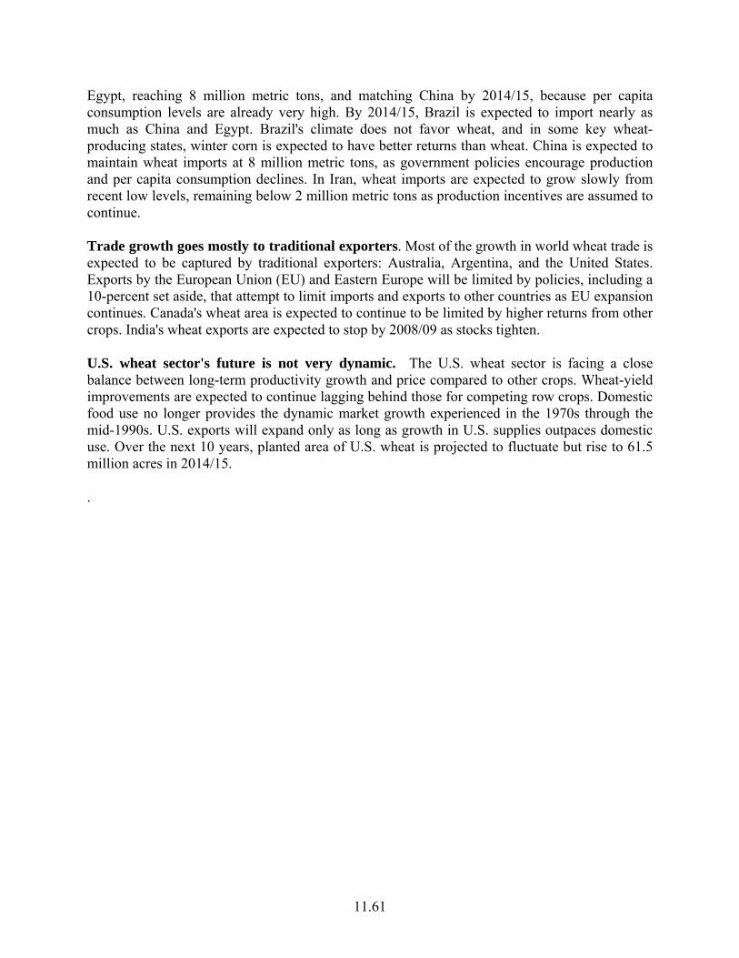
11.61

Egypt, reaching 8 million metric tons, and matching China by 2014/15, because per capita consumption levels are already very high. By 2014/15, Brazil is expected to import nearly as much as China and Egypt. Brazil's climate does not favor wheat, and in some key wheat-producing states, winter corn is expected to have better returns than wheat. China is expected to maintain wheat imports at 8 million metric tons, as government policies encourage production and per capita consumption declines. In Iran, wheat imports are expected to grow slowly from recent low levels, remaining below 2 million metric tons as production incentives are assumed to continue.

Trade growth goes mostly to traditional exporters. Most of the growth in world wheat trade is expected to be captured by traditional exporters: Australia, Argentina, and the United States. Exports by the European Union (EU) and Eastern Europe will be limited by policies, including a 10-percent set aside, that attempt to limit imports and exports to other countries as EU expansion continues. Canada's wheat area is expected to continue to be limited by higher returns from other crops. India's wheat exports are expected to stop by 2008/09 as stocks tighten.

U.S. wheat sector's future is not very dynamic. The U.S. wheat sector is facing a close balance between long-term productivity growth and price compared to other crops. Wheat-yield improvements are expected to continue lagging behind those for competing row crops. Domestic food use no longer provides the dynamic market growth experienced in the 1970s through the mid-1990s. U.S. exports will expand only as long as growth in U.S. supplies outpaces domestic use. Over the next 10 years, planted area of U.S. wheat is projected to fluctuate but rise to 61.5 million acres in 2014/15.

.

11.62

Table 2. USDA-ERS Projected U.S. Wheat Supply and Demand (March 14, 2005) U.S. wheat baseline

Item 2004/05 2005/06 2006/07 2007/08 2008/09 2009/10 2010/11 2011/12 2012/13 2013/14 2014/15

Area (million acres):

Planted acres 59.7 60.0 58.5 58.5 59.0 59.5 60.0 60.0 61.0 61.0 61.5

Harvested acres 50.0 51.0 49.7 49.7 50.2 50.6 51.0 51.0 51.9 51.9 52.3

Yields (bushels per acre):

Yield/harvested acre 43.2 42.3 42.7 43.1 43.5 43.9 44.3 44.7 45.1 45.5 45.9

Supply(million bushels):

Beginning stocks 547 568 638 648 647 626 609 597 569 571 557

Production 2,158 2,155 2,120 2,140 2,185 2,220 2,260 2,280 2,340 2,360 2,400

Imports 65 65 70 70 70 70 75 75 75 75 75

Supply 2,770 2,788 2,828 2,858 2,902 2,916 2,944 2,952 2,984 3,006 3,032

Use (million bushels):

Food 920 920 925 930 935 940 945 950 955 960 965

Seed 82 80 80 81 81 82 82 83 83 84 84

Feed & residual 225 200 200 200 210 210 220 225 225 230 230

Domestic 1,227 1,200 1,205 1,211 1,226 1,232 1,247 1,258 1,263 1,274 1,279

Exports 975 950 975 1,000 1,050 1,075 1,100 1,125 1,150 1,175 1,200

Total use 2,202 2,150 2,180 2,211 2,276 2,307 2,347 2,383 2,413 2,449 2,479

Ending stocks 568 638 648 647 626 609 597 569 571 557 553

Stocks/use ratio, percent 25.8 29.7 29.7 29.3 27.5 26.4 25.4 23.9 23.7 22.7 22.3

Prices (dollars per bushel):

Farm price 3.35 3.00 3.05 3.15 3.25 3.35 3.40 3.50 3.50 3.55 3.60

Loan rate 2.75 2.75 2.75 2.75 2.75 2.75 2.75 2.75 2.75 2.75 2.75

Variable costs of production (dollars):

Per acre 73.08 74.65 75.67 76.37 77.09 77.89 78.77 79.68 80.61 81.54 82.49

Per bushel 1.69 1.76 1.77 1.77 1.77 1.77 1.78 1.78 1.79 1.79 1.80

Returns over variable costs (dollars per acre):

Net returns 1/ 71.64 54.37 54.56 59.40 64.28 69.18 71.85 76.77 77.24 79.99 82.75

1/ Net returns include estimates of marketing loan benefits.

Source: http://www.ers.usda.gov/publications/oce051/oce20051c.pdf

11.63

Strategic Marketing Plan Worksheet 6 (Continued) Market Outlook & Expectations – Grain Sorghum

Source: http://www.ers.usda.gov/Briefing/Corn/2005baseline.htm

USDA feed grains baseline, 2005-14

The gross domestic product is expected to grow in the United States and around the world, raising incomes and boosting demand for meat. A growing livestock industry will need increasing supplies of feed grains. A ban on methyl tertiary butyl ether (MTBE) in some States is boosting the use of ethanol in gasoline to comply with the Clean Air Act's requirement for oxygenates in the fuel. The majority of ethanol is made from grains, creating an increasing use for feed grains. Estimated net returns per acre are expected to be more favorable for corn than for other feed grains. As a result, acres planted to corn, the primary feed grain in the United States, are forecast to increase slightly. In contrast, plantings of oats may remain unchanged, but sorghum and barley acres may decline. The effect of these changes, as well as other factors, on the U.S. feed grains sector are evaluated in preparation of the Department's 10-year baseline projection.

Each year, USDA updates its 10-year projection of supply and utilization of major field crops grown in the United States, including feed grains. The commodity projections are used to forecast farm program costs and to prepare the President's budget. One key use of the projections is as a "baseline" from which to analyze the impacts of potential policy changes affecting U.S. agriculture. This discussion briefly summarizes the analysis underlying the feed grain projections for 2005-14.

The U.S. feed grain sector is expected to face a period of firm growth during the entire baseline period as growing economies throughout the world encourage consumption of livestock products. Ethanol for fuel will also boost corn use and, to some extent, sorghum use. Corn will continue as the feed grain of choice, because of rising yields, especially in the United States. Sorghum, barley, and oats will continue as specialty crops.

Increased global demand for meat is expected to boost world consumption of feed grains. However, production constraints, especially limited area, will keep many traditional grain-importing countries from expanding production as rapidly as use, boosting global coarse grain trade. Most of the growth is in corn trade, and the U.S. share of corn trade is expected to increase. Global barley trade is also expected to expand, but remain small. Sorghum trade is expected to decline due to reduced imports by Mexico, but later regain initial trade levels.

Supply

Supply reflects changes in land used for planting and gains in yields of the crops.

Corn acres to increase. The number of acres planted to corn is expected to total 81 million in 2005 and increase to 84 million by the end of the baseline. Corn plantings are influenced by

11.64

expected net returns for corn relative to competing crops. Net returns are determined by yields, production costs, and prices. However, the number of acres available for crop plantings is limited. If more water were available for irrigation, additional land could be brought into production but that is not foreseen. As a result, feed grains compete for acres with other crops.

Among the feed grains, corn has the highest return above variable costs. Soybeans are the major competitor with corn and had returns above corn from 1996/97 through 2001/02. Net returns for soybeans are expected to be below net returns for corn throughout the baseline period, due to lower relative prices caused by increased South American production.

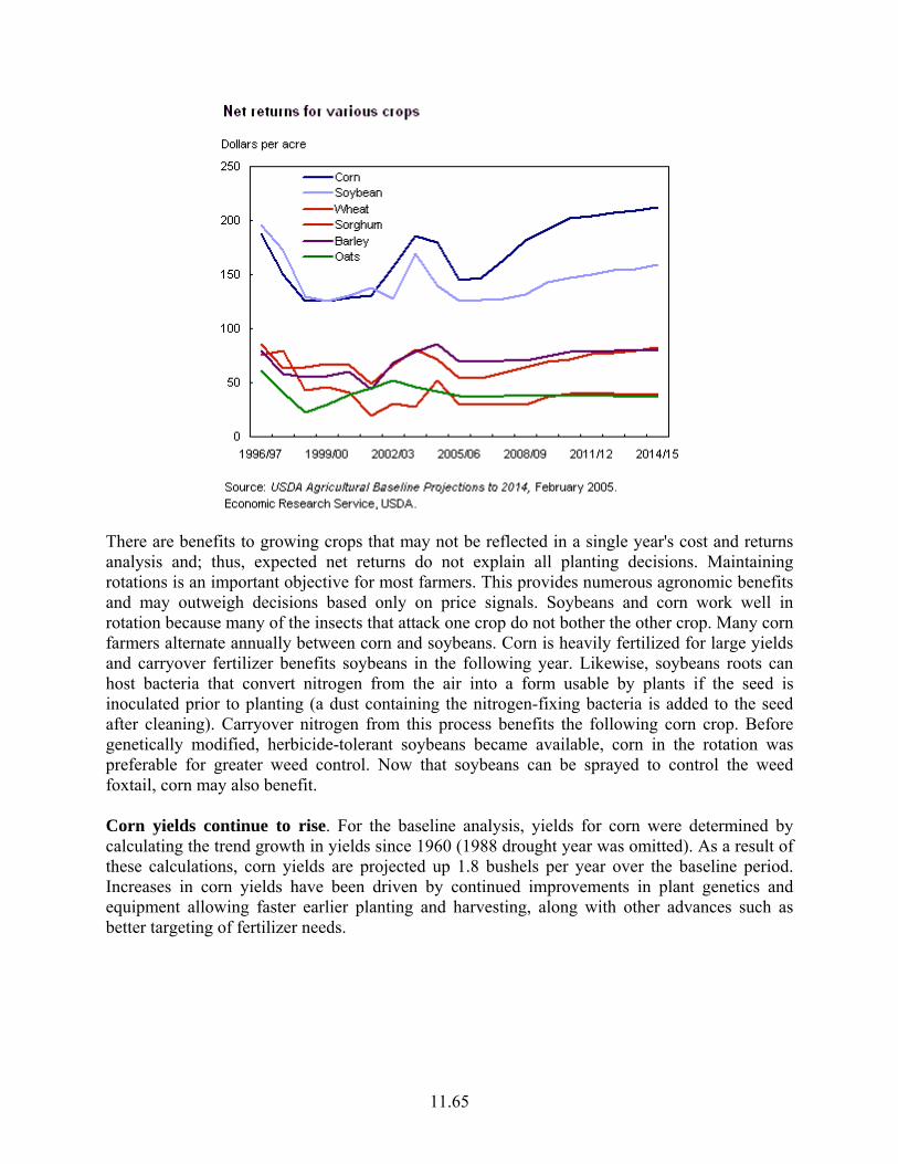
11.65

There are benefits to growing crops that may not be reflected in a single year's cost and returns analysis and; thus, expected net returns do not explain all planting decisions. Maintaining rotations is an important objective for most farmers. This provides numerous agronomic benefits and may outweigh decisions based only on price signals. Soybeans and corn work well in rotation because many of the insects that attack one crop do not bother the other crop. Many corn farmers alternate annually between corn and soybeans. Corn is heavily fertilized for large yields and carryover fertilizer benefits soybeans in the following year. Likewise, soybeans roots can host bacteria that convert nitrogen from the air into a form usable by plants if the seed is inoculated prior to planting (a dust containing the nitrogen-fixing bacteria is added to the seed after cleaning). Carryover nitrogen from this process benefits the following corn crop. Before genetically modified, herbicide-tolerant soybeans became available, corn in the rotation was preferable for greater weed control. Now that soybeans can be sprayed to control the weed foxtail, corn may also benefit.

Corn yields continue to rise. For the baseline analysis, yields for corn were determined by calculating the trend growth in yields since 1960 (1988 drought year was omitted). As a result of these calculations, corn yields are projected up 1.8 bushels per year over the baseline period. Increases in corn yields have been driven by continued improvements in plant genetics and equipment allowing faster earlier planting and harvesting, along with other advances such as better targeting of fertilizer needs.

11.66

A similar analysis with 1988 included was performed for barley and oats, but their growth is considerably slower than corn. Barley yields are projected up by 0.6 bushels per year, while oats yields are up 0.4 bushels per year. Sorghum yields, based on a 10-year average, are expected to increase by 0.4 or 0.5 bushels per year.

Demand

Demand for feed grains is derived from the demand for livestock feed, which is derived from the demand for meat, milk, and eggs.

Macroeconomic growth indirectly affects feed grain use. The baseline assumes that growth in U.S. gross domestic product (GDP) moderates in the near term from the rapid growth in 2004 as the economy moves toward a longrun annual growth rate near 3 percent. Ongoing U.S. technological advances associated with computing and telecommunications will provide support for worldwide economic growth throughout the projection period.

World economic growth is projected to strengthen from the slow growth of 2001-03, averaging over 3 percent through 2014. Most countries of the world move close to longrun sustainable economic growth rates. Relatively high oil prices in 2004 and beyond will constrain Asia and its manufacturing sector, which is far more dependent on energy for GDP growth than more developed economies.

11.67

As economies expand, consumers shift to more meat in their diets and this requires more feed grains for meat production. Diets in the United States already have adequate quantities of meat, but an expanding economy will keep meat consumption brisk. Internationally, expanding economies are likely to change diets, especially in developing economies. As a result, the baseline analysis expands world trade in feed grains and increases exports from the United States.

11.68

Livestock products to increase, boosting feed grain use. Production of U.S. livestock products is expected to increase during the baseline period. U.S. beef production was down in 2004 because of reduced cattle numbers in prior years and small calf crops. In addition, with normal weather, heifers are likely to be held back to rebuild the herds. The combination of a small calf crop and larger numbers of replacement heifers will slow beef production increases in 2006. Beginning in 2007, beef production will continue increasing through the end of the baseline period. As increased numbers of cattle go on feed, more feed grains will be needed.

11.69

Pork production in 2005 is expected to be up 1 percent from 2004, and then continue increasing through 2014. The greatest gains are forecast for 2006 at 1.8 percent per year and 2008 at 1.5 percent. Production may slow during the remainder of the baseline period, but still rise nearly 1 percent per year. The increase in hog numbers will necessitate more feed grains, primarily corn.

Broiler production is projected to increase throughout the baseline period. With beef production down in 2004, broiler production was up 4.2 percent. But growth will slow to about 3 percent per year during the baseline. Thus, feed needs for the broiler industry are expected to grow over the period.

Feed needs for turkey and egg producers are also expected to increase during the baseline period. Projected turkey production is expected to be up about 2 percent annually during 2005-14. Egg production is projected to increase about 1 percent per year during the period.

Milk production is projected to increase slowly, around 2 percent annually through 2007/08, and then decline to near 1 percent growth in the out years. Dairy cow numbers are expected to continue their long-term decline throughout the baseline period. Production gains are the result of increased production per cow. As a result, feed needs are likely to increase.

Ethanol use continues to grow. Corn used for producing fuel alcohol has grown sharply since the early 1980s. As a result, fuel alcohol has become the largest component within the food, seed, and industrial (FSI) use category. The volume of total FSI has overtaken even corn exports in recent years. Corn's use in fuel alcohol production depends on the interaction of government incentives and policies, technology development, corn prices, prices of coproducts from ethanol production, and prices of energy substitutes.

11.70

Ethanol production expanded very rapidly until marketing year 1995/96 (September-August), when there was a major contraction due to tight corn supplies and record high corn prices. Since then, ethanol output has rebounded, especially since methyl tertiary butyl ether (MTBE), a competing oxygenate produced from methyl alcohol, was banned in many States and policies have encouraged ethanol use.

Policies are very important for the expansion of ethanol production. A federal tax credit for ethanol blending, currently 51 cents per gallon, is assumed to continue. However, the biggest factor underlying the recent expansion has been the adoption of ethanol by California, the Nation's largest gasoline market, after it prohibited the use of MTBE. The need to ramp up production to meet mandated use has boosted production, especially since New York and Connecticut have also banned MTBE. Ethanol is the principal replacement oxygenate where reformulated gasoline is used, requiring 2-percent oxygen by weight.

Policy-influenced market conditions are also critical determinants of ethanol production. More than half of all fuel ethanol is blended into conventional gasoline as a fuel or octane enhancer. Prices of ethanol relative to gasoline prices are a key component for determining how much ethanol is blended. The remaining ethanol is used for blending into reformulated gasoline, which will be important in California, New York, and Connecticut. It is also used in oxygenated gasoline for the winter carbon monoxide program. (The program requires the use of oxygenated gasoline for designated winter months. The intent of the oxygenate is to offset the increased carbon dioxide levels emitted from gasoline engines due to hard starting and lengthy warm-up periods in cold weather).

While use of oxygenates largely results from mandated clean air requirements, fuel producers can choose among competing oxygenates based on their relative prices. Some States offer incentives that also influence demand for ethanol. For instance, Illinois has a sales tax exemption for ethanol, while Minnesota has mandated a year-round minimum oxygen content requirement for all gasoline sold.

Baseline projections for U.S. feed grains supply and use

U.S. feed grain supplies and use are expected to increase over the baseline period, after a drop in 2005/06 from 2004/05 (because the trend yields used in the analysis are lower than the actual yields for 2004).

Most production gains expected from productivity. Feed grain production increases throughout the projection period, as yield growth accounts for most of the expanded output. Corn is expected to gain in share of total feed grain production and use. Corn area is projected to experience moderate growth over the baseline period and oats may remain unchanged. Sorghum and barley plantings are expected to decline slowly. Net returns for all four feed grains decline sharply the first year of the baseline because the trend yields used in the analysis are lower than the actual yields for 2004. Net returns for oats are nearly constant during the projection period, while net returns for corn, sorghum, and barley increase.

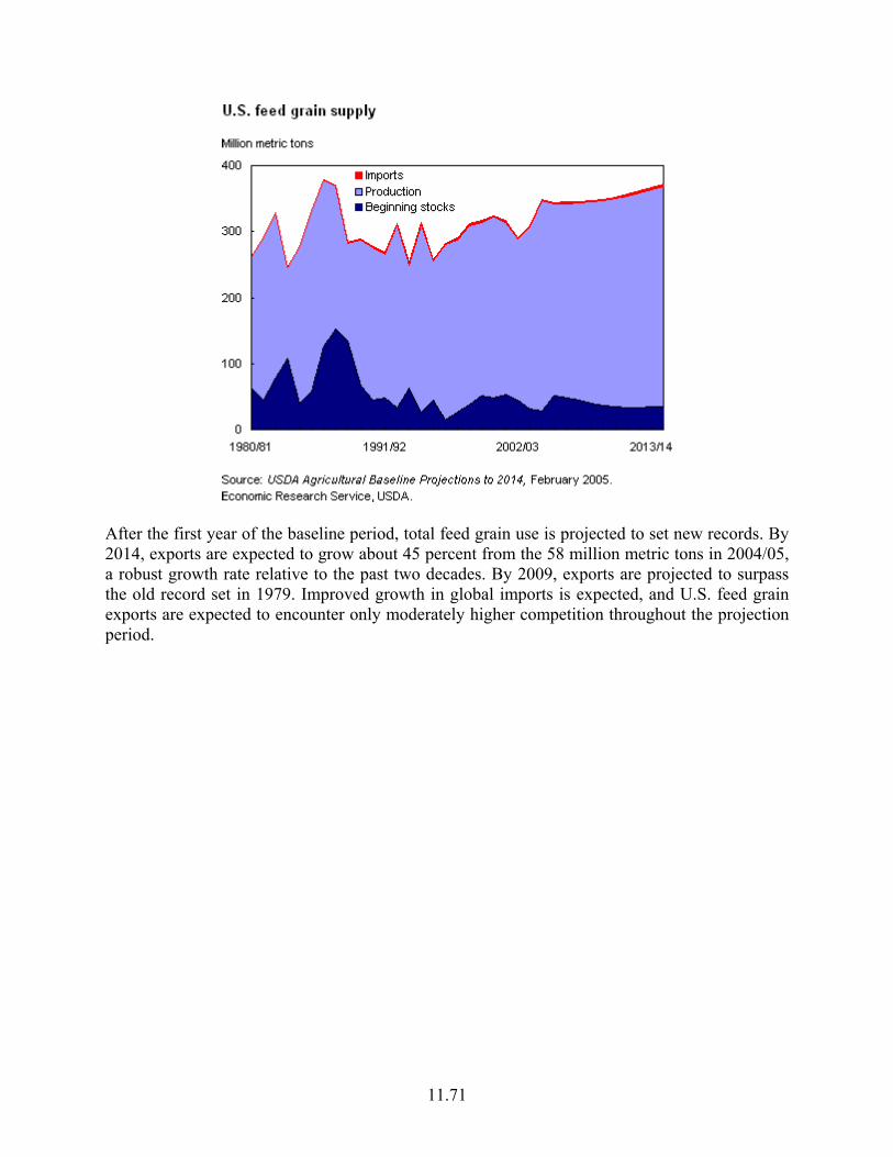
11.71

After the first year of the baseline period, total feed grain use is projected to set new records. By 2014, exports are expected to grow about 45 percent from the 58 million metric tons in 2004/05, a robust growth rate relative to the past two decades. By 2009, exports are projected to surpass the old record set in 1979. Improved growth in global imports is expected, and U.S. feed grain exports are expected to encounter only moderately higher competition throughout the projection period.

11.72

U.S. ending stocks of feed grains are projected to decline slowly until 2011/12 then increase and remain between 34 and 35 million metric tons. These ending stocks are slightly below the average ending stocks in the 1990s of 41 million metric tons. Productivity is projected to account for most of production growth, with the remainder coming from increased plantings.

Corn supply and use to grow. Corn area is expected to grow and yields increase, resulting in new record corn production. Use will likely also set records as livestock herds grow, raising feed needs, and industrial uses for corn expand. China becomes a net importer in 2007/08, contributing to projected exports of U.S. corn increasing throughout the baseline.

Corn prices in 2005/06 are expected to be higher than in 2004/05, reflecting supply growing less than total use. At the onset of the baseline, domestic corn use is strong, and continues expanding throughout the period. U.S. corn exports are also expected to grow. The U.S. share of global corn trade is expected to increase, mostly because of reduced exports and increased imports by China. Global corn trade is expected to grow, given rising global meat demand.

Planted area for corn is projected to remain relatively large and grow slowly over the baseline period, as use strengthens and prices improve. Corn competes mostly with soybeans for land and is used extensively in rotations with soybeans. Corn area grows relative to soybean area, as relative net returns are expected to favor corn throughout most of the baseline.

Gains in corn yields are expected to continue over the entire baseline period, facilitated by genetic improvements. Corn production is projected to increase, setting new records.

11.73

Increasing meat production boosts feed and residual use. Feed and residual use is expected to decline in 2005/06, the initial year, but grow throughout the remainder of the projection period. Increasing U.S. meat production and associated livestock (measured by grain-consuming animal units) account for the rising use of grain.

Despite its growth, direct feed use of corn is not as strong as it would be without coproducts from ethanol production. Ethanol wet mills produce corn gluten feed, corn gluten meal, and corn oil as coproducts, while dry mills produce distiller's dried grains (DDG). The baseline assumes that each 56-pound bushel of corn that goes into dry-mill ethanol production results in 17.5 pounds of DDG as a coproduct. The protein content of DDG for beef cattle is about 23 percent, compared to 48 percent for soybean meal and about 10 percent for corn. The energy content of DDG falls between that of corn and soybean meal. Thus, the baseline assumes that the DDG coproduct of dry-mill ethanol production substitutes for about a 50-50 split of corn and soybean meal in feed rations, or about 8.75 pounds each of corn and soybean meal for each bushel of corn used for ethanol production.

Ethanol production keeps corn use high. Food, seed, and industrial (FSI) use of corn is anticipated to increase throughout the baseline period, beginning at a record level. Major growth is expected in ethanol use because many States are banning MTBE and ethanol is its principal replacement. Greater corn use is projected in the baseline as the ethanol industry expands production. Gains for high fructose corn syrup (HFCS) and most other food and industrial components are projected to be smaller than in the previous decade. Food and starch, other segments of FSI use, are mature markets and projected gains largely reflect population growth.

11.74

Projected exports demonstrate growth compared with the 1980s and 1990s, but remain below the record established in 1979/80 until the middle of the forecast period. World corn imports grow because of increased meat production.

Ending stocks of corn are expected to decline to around 1.1 billion bushels toward the later part of the baseline period, but then increase. Prices strengthen from lows in the early 2000s to $2.45 per bushel toward the end of the projection period, as the stocks-to-use ratio declines slightly.

11.75

Sorghum supply to remain about steady. Growth in sorghum production is expected to equal use, resulting in nearly constant ending stocks. Acres planted are expected to decline only slightly, but yields increase. Feed and residual use will vary depending upon supply, but food, seed, and industrial use (primarily ethanol production) will increase.

Sorghum production is projected to grow to 450 million bushels by 2014. This reflects a slight decline in plantings but trend yield growth of 0.4 to 0.5 bushels per year. Despite the projected yield growth during the baseline period, yields are not expected to exceed 1994's record of 72.7 bushels per acre.

Sorghum exports decline during the baseline, especially in 2006-08 when reduced tariffs on corn trade with Mexico lead to higher U.S. corn exports and lower sorghum shipments. With reduced U.S. sorghum exports, increased feed and residual use is projected. Food, seed, and industrial use rises slowly in the baseline, remaining record high due to growth in ethanol production.

Barley supplies increase modestly. Rising yields are expected to modestly increase barley production, reaching 255 million bushels by 2014. Planted acreage declines slightly over the period, as barley's net returns cannot compete for more area. Yield per acre is expected to increase 0.6 bushels over the period, in line with trend increases.

Food, seed, and industrial use was held steady over the baseline, mainly because beer production in the United States is expected to level off. Barley feed and residual use increases slightly during the baseline period in line with production. Barley exports are projected to be 15 million bushels per year, as shipments of feed barley to the Middle East continue. Imports are expected to remain unchanged at 25 million bushels, because of malting barley imports from Canada. The

11.76

average barley price is projected to rise through the baseline, reaching $2.65 per bushel by the end of the period.

Oats plantings unchanged. Supplies grow modestly as increased yields and oat imports, principally from Canada, supplement domestic oats production. Food, seed, and industrial use is expected to remain unchanged, with some rise in feed and residual use, keeping ending stocks relatively constant.

The declining long-term trend in oat acreage is projected to stabilize. With oat plantings expected to remain constant during the baseline period, slow growth in yields results in a 5 million bushel increase in production by the end of the period. The crop will remain important in some rotations and as a cover crop. There is also some modest growth in imports. Supplies drop in the beginning year of the baseline because plantings and yields decline. Supplies grow in subsequent years of the baseline, but do not reach the levels of 2004/05. Total use starts at 186 million bushels, increasing to 196 million due to higher feed use. Imports rise from 85 million bushels to 95 million, or 36-37 percent of supply, making up the difference between production and use. Feed and residual use ranges from 110 million bushels to 120 million. Oat prices increase over the baseline period, and imports supplement domestic supplies.

Baseline projections for world feed grains trade

The USDA baseline also provides projections for global trends in feed grain supply, use, and trade.

Expanding consumption to boost corn trade. Increased global demand for meat is expected to boost world consumption of feed grains. However, production constraints, especially limited area, will keep many traditional importing countries from expanding production as rapidly as use, boosting global trade from 102 million metric tons in 2005/06 to 131 million in 2014/15. Most of the growth is in corn trade, up from 78 million metric tons in 2005/06 to 104 in 2014/15. The U.S. share of corn trade is expected to increase from 70.9 percent during 2005/06 to 72.7 percent by the end of the projection period.

11.77

As recently as 2002/03, China was the second largest corn exporter. China, however, is expected to limit exports and gradually increase imports of corn, becoming a net importer by 2007/08. Corn area expansion in Argentina is expected to be limited by profitable returns for soybeans. Area expansion is also expected to be limited in other exporting countries such as South Africa and Thailand. As Eastern European countries like Hungary join the European Union (EU), less corn is exported outside of Europe. However, Brazil is expected to remain a significant net exporter of corn because of attractive world prices and niche marketing.

China is key to the future of global corn trade. In recent years, China has maintained corn exports, while reducing stocks when production fell below domestic use. Chinese stocks are now thought to be reduced to levels that will limit future stock declines because they would likely boost internal prices. Meat demand in China is expected to rise because of strong income growth. Rapid gains in meat production are expected to increase corn feed use. While corn yield growth is projected to rise less than 1 percent per year, area increases will be limited by higher returns from other land uses. So by 2007, China becomes a net importer of corn. Nonetheless, northeast China is expected to remain a surplus corn producing region and, because it is so close to South Korea—one of the world's largest corn importers—China is expected to continue exporting corn. However, southern China is further away, and is expected to be an increasingly corn deficit region, boosting imports during the baseline period.

Growth in global corn imports over the baseline period is not limited to China. Most corn importing countries are expected to increase imports as meat production rises because of factors that limit the growth in corn production. The largest increase in corn imports is expected for Mexico, where a switch from sorghum to corn is expected on top of strong growth in meat production. Imports by the rest of Latin America are expected to grow only modestly, at about the pace of population growth. With stronger economic growth, Egypt is expected to lead the

11.78

growth in corn imports by North Africa and the Middle East. With limited barley area, and increasing barley exports, Canada is expected to increase corn imports to support meat production increases. Russia and other former Soviet Union countries increase corn imports faster than Ukraine increases exports, making the region a growing net importer of corn. However, some markets, like Japan, are expected to reduce imports due to slow growth in meat consumption combined with higher meat imports.

Barley trade to expand. Global barley is expected to expand slowly, from 15 million metric tons in 2005/06 to over 17 million by the end of the baseline. Demand for feed barley is expected to grow in North Africa and the Middle East, where production increases are limited by the climate, but imports by Saudi Arabia are expected to be nearly flat. Imports of barley by Saudi Arabia depend on rainfall and grazing for sheep and camels. China leads import growth in barley for malting. EU stocks are expected to limit the pressure to subsidize EU barley exports, so EU barley exports are expected to remain near 3 million metric tons throughout the baseline. Barley exports by Australia, Canada, and Ukraine are expected to increase. U.S. barley trade is expected to remain small.

Sorghum trade to decline. Sorghum trade is expected to decline from nearly 7 million metric tons in 2005/06 to less than 6 million in 2008/09 because of reduced imports by Mexico, but then show some recovery by the end of the baseline. Mexico's current system of variable rate quotas for corn with "cupos" for over quota imports tends to discourage corn imports and boost sorghum imports that do not have quotas. However, under the North American Free Trade Agreement, Mexican corn tariffs are phased down and disappear by 2008. As corn tariffs are reduced and then eliminated, Mexican feed compounders are expected to shift to corn, away from sorghum. Japan is also expected to reduce sorghum imports slightly as feed grain imports decline.

Other coarse grain trade is expected to grow very slowly over the baseline period, with a small increase in oats trade nearly offset by reduced rye trade. EU policy is expected to maintain oat production and exports, but a drop in EU rye production (due to reforms of the EU's Common Agricultural Policy that ended rye intervention prices) and exports is expected. Canada will remain the main supplier of imported oats to the U.S. market.

Industry prospects are good. Yields per acre for U.S. feed grains will continue to increase, and corn yields will grow at the fastest rate. Rising corn yields help boost net returns, keeping planted area up. Slower yield growth for barley and other feed grains makes them less attractive to producers, leading to a slight decline or no change in acres planted over the period. Corn production is projected up 16 percent over the 2005-14 period, sorghum is up 3 percent, barley up 6 percent, and oats are up 5 percent.

Strong use both domestically and worldwide keeps feed grain prices above U.S. loan rates during most of the baseline, reducing government farm program costs. Use of corn for corn sweeteners is expected to grow at the rate of population increase. Use of corn to produce ethanol for fuel will continue to climb. Feed and residual use will also expand over the period as livestock and poultry production continue to increase.

11.79

Increased global demand for meat is expected to boost world consumption of feed grains. Global trade in feed grains is expected to rise because many traditional importing countries will not be able to increase production as much as the gains in consumption. Most of the growth in trade is in corn and the U.S. share of the market is expected to increase.

11.80

Table 3. USDA-ERS Projected U.S. Grain Sorghum Supply and Demand (March 14, 2005) U.S. sorghum baseline

Item 2003/04 2004/05 2005/06 2006/07 2007/08 2008/09 2009/10 2010/11 2011/12 2012/13 2013/14 2014/15

Area (million acres):

Planted acres 9.4 7.5 8.4 8.4 8.4 8.4 8.3 8.3 8.3 8.2 8.2 8.2

Harvested acres 7.8 6.6 7.0 7.0 7.0 7.0 6.9 6.9 6.9 6.8 6.8 6.8

Yields (bushels per acre):

Yield/harvested acre 52.7 71.9 62.5 63.0 63.4 63.9 64.3 64.8 65.2 65.7 66.1 66.6

Supply and use (million bushels):

Beginning stocks 43 34 60 60 58 58 58 58 56 61 59 59

Production 411 472 440 440 445 445 445 445 450 445 450 455

Imports 0 0 0 0 0 0 0 0 0 0 0 0

Supply 454 505 500 500 503 503 503 503 506 506 509 514

Use (million bushels):

Feed & residual 200 195 165 175 190 200 190 185 180 175 170 165 Food, seed, & industrial 20 50 50 52 55 60 60 62 65 67 70 72

Domestic 220 245 215 227 245 260 250 247 245 242 240 237

Exports 201 200 225 215 200 185 195 200 200 205 210 215

Total use 421 445 440 442 445 445 445 447 445 447 450 452

Ending stocks 34 60 60 58 58 58 58 56 61 59 59 62 Stocks/use ratio, percent 8.1 13.5 13.6 13.1 13.0 13.0 13.0 12.5 13.7 13.2 13.1 13.7

Prices (dollars per bushel):

Farm price 2.39 1.75 1.85 2.00 2.10 2.20 2.25 2.30 2.30 2.30 2.30 2.30

Loan rate 1.98 1.95 1.95 1.95 1.95 1.95 1.95 1.95 1.95 1.95 1.95 1.95

Variable costs of production (dollars):

Per acre 97.94 102.83 105.26 106.08 106.58 107.38 108.33 109.46 110.61 111.78 112.96 114.17

Per bushel 1.86 1.43 1.68 1.68 1.68 1.68 1.68 1.69 1.70 1.70 1.71 1.71

Returns over variable costs (dollars per acre):

Net returns 1/ 28.01 51.76 29.11 29.37 29.73 33.20 36.35 39.58 39.35 39.33 39.07 39.01

1/ Net returns include estimates of marketing loan benefits.

Source: http://www.ers.usda.gov/publications/oce051/oce20051c.pdf

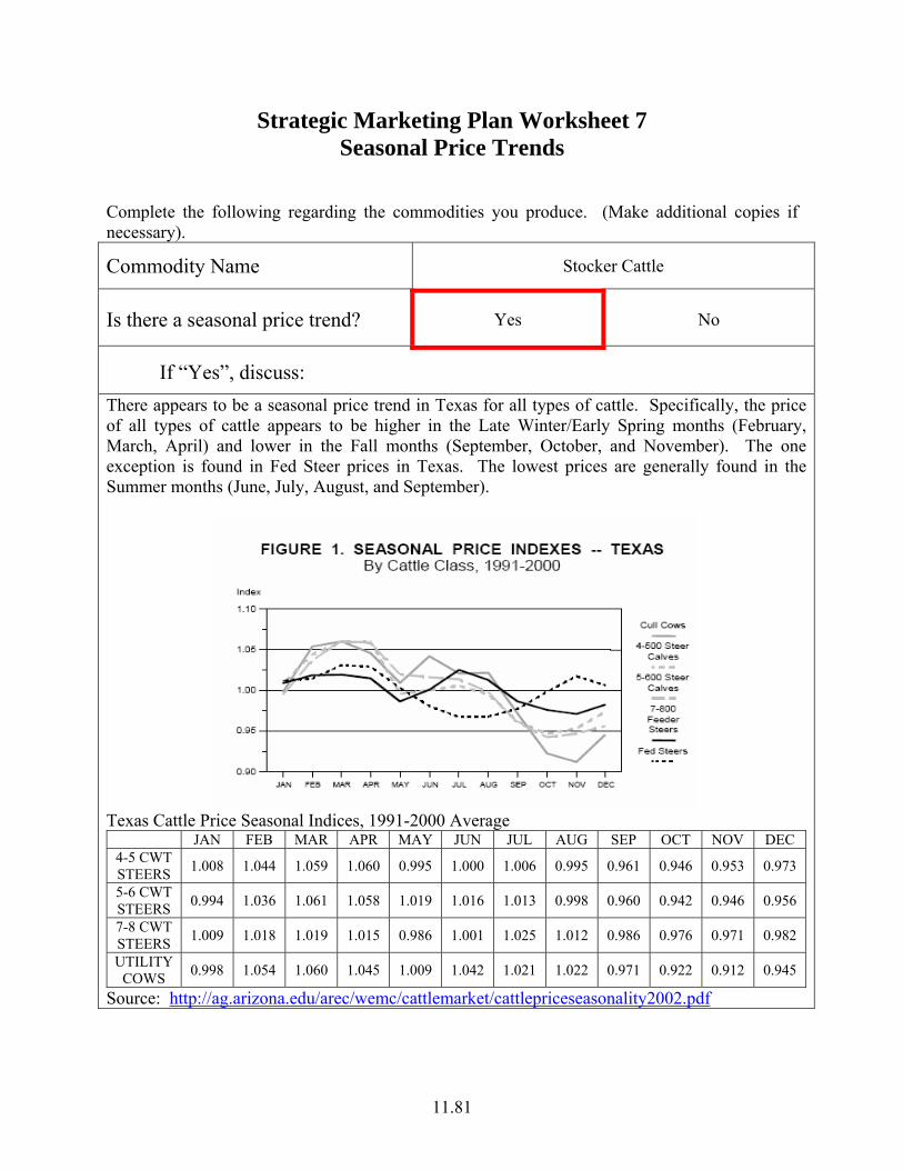
11.81

Strategic Marketing Plan Worksheet 7 Seasonal Price Trends


Commodity Name Stocker Cattle


If “Yes”, discuss: There appears to be a seasonal price trend in Texas for all types of cattle. Specifically, the price of all types of cattle appears to be higher in the Late Winter/Early Spring months (February, March, April) and lower in the Fall months (September, October, and November). The one exception is found in Fed Steer prices in Texas. The lowest prices are generally found in the Summer months (June, July, August, and September).

Texas Cattle Price Seasonal Indices, 1991-2000 Average

JAN FEB MAR APR MAY JUN JUL AUG SEP OCT NOV DEC 4-5 CWT STEERS 1.008 1.044 1.059 1.060 0.995 1.000 1.006 0.995 0.961 0.946 0.953 0.973

5-6 CWT STEERS 0.994 1.036 1.061 1.058 1.019 1.016 1.013 0.998 0.960 0.942 0.946 0.956

7-8 CWT STEERS 1.009 1.018 1.019 1.015 0.986 1.001 1.025 1.012 0.986 0.976 0.971 0.982

UTILITY COWS 0.998 1.054 1.060 1.045 1.009 1.042 1.021 1.022 0.971 0.922 0.912 0.945

Source: http://ag.arizona.edu/arec/wemc/cattlemarket/cattlepriceseasonality2002.pdf

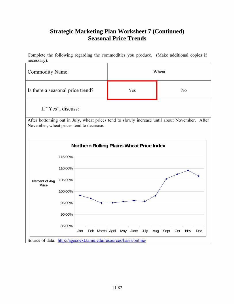
11.82

Strategic Marketing Plan Worksheet 7 (Continued) Seasonal Price Trends


Commodity Name Wheat


If “Yes”, discuss:

After bottoming out in July, wheat prices tend to slowly increase until about November. After November, wheat prices tend to decrease.

Northern Rolling Plains Wheat Price Index

85.00%

90.00%

95.00%

100.00%

105.00%

110.00%

115.00%

Jan Feb March April May June July Aug Sept Oct Nov Dec

Percent of Avg Price

Source of data: http://agecoext.tamu.edu/resources/basis/online/

11.83

Strategic Marketing Plan Worksheet 7 (Continued) Seasonal Price Trends


Commodity Name Grain Sorghum


If “Yes”, discuss: The corn market (used as a substitute for grain sorghum) appears to gradually increase from late August until January. From January through April (where it reaches its maximum), corn prices increase at a faster rate. After April, the market price decreases reaching a bottom in late July/early August.

Fort Worth Corn Price Index

50.00%

60.00%

70.00%

80.00%

90.00%

100.00%

110.00%

120.00%

130.00%

Jan

Feb

March

April

MayJu

ne July

Augu

stSe

pt Oct Nov Dec

Percent of Average Price

Source of data: http://agecoext.tamu.edu/resources/basis/online/

11.84

Strategic Marketing Plan Worksheet 9 Available Price Risk Tools - Livestock



Check all alternatives

available for this commodity &

you are comfortable with using

Explain Those

Without Checks.

Cash Market (Auction Barn) √

Private Treaty √

Telephone, Video, & Satellite Auction √

Forward Contract √

Retained Ownership √

Basis Contract Don’t Understand

Minimum Price Contract √

Grid Pricing √

Hedging in Futures Markets Don’t Understand

Options Markets Don’t Understand

Farm Program √

Cooperatives/Groups √


Stocker Cattle

11.85

Strategic Marketing Plan Worksheet 8 Available Price Risk Tools - Crops







Cash Market at Harvest √

Speculative Storage I do not have the storage facilities.


Hedge to Arrive Contract Don’t Understand

Basis Contract Don’t Understand

Minimum Price Contract √

Hedging in Futures Markets Don’t Understand.

Options Markets Don’t Understand.

Farm Program √

Cooperatives/Groups √


Wheat

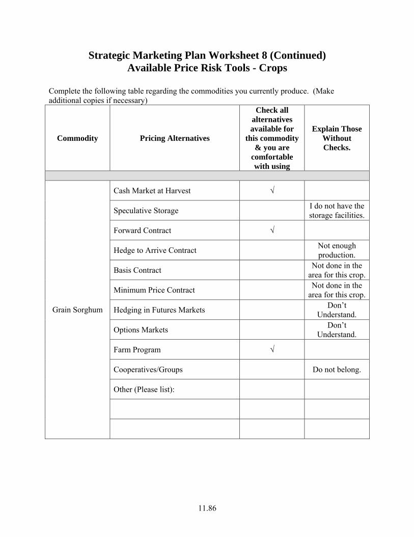
11.86

Strategic Marketing Plan Worksheet 8 (Continued) Available Price Risk Tools - Crops







Cash Market at Harvest √

Speculative Storage I do not have the storage facilities.


Hedge to Arrive Contract Not enough production.

Basis Contract Not done in the area for this crop.

Minimum Price Contract Not done in the area for this crop.

Hedging in Futures Markets Don’t Understand.

Options Markets Don’t Understand.

Farm Program √

Cooperatives/Groups Do not belong.


Grain Sorghum

11.87

Strategic Marketing Plan Worksheet 10 Projected Marketing Schedule

Month/Strategy

Commodity Jan Feb Mar Apr May Jun Jul Aug Sept Oct Nov Dec

Stocker Cattle

Lock in price for 40% of Prod.


Cash Sales

Wheat



Cash Sales

Grain Sorghum Cash

Sales

11.88

Strategic Marketing Plan Worksheet 11 Evaluating the Plan

Evaluate the marketing actions taken during the last year. (Make additional copies if necessary)

Commodity Action Taken Last Year

Success/Failure of the Plan Explanation

Stocker Cattle Sold cash cattle in May 2004 Success

I lucked out. Cattle prices began rising in mid-April 2004. The cash market ended up settling at $105/cwt in May. However, I was unprotected for the entire year. If the market had gone the other way, I would have not realized such a return.

Wheat Sold cash wheat in May 2004

Mildly Successful

Cash wheat sold for $3.19/bu. It had reached a high of $3.84 and a low of $3.03. After May 2004, the wheat price continued to slide downward. Therefore, I could have taken advantage of higher prices with some price risk management tools, however I did not sell at the bottom. Furthermore, storage would not have helped me this year.

Grain Sorghum Sold cash

sorghum in October 2004

Success & Failure

Grain sorghum is used to just generate cash flow. It is not a primary crop, and doesn’t utilize many acres. Because of this, our options are limited.

11.89

Case Study Tactical Marketing Plan

Worksheets

11.90

Tactical Marketing Plan Worksheet 1 Decision Making Information

Complete the following table regarding the commodities you currently produce under current market conditions. (Make additional copies if necessary). Commodity Stocker Cattle Expected Yearly Production

(Raised Stocker Cattle) (Purchased Stocker Cattle)

2,921.40 cwt (2,171.40 cwt) (750.00 cwt)

Variable Cost of Production per Unit


$88.25/cwt ($82.39/cwt)

($105.25/cwt) Total Cost of Production (Break-Even)


$93.77/cwt ($87.75/cwt)

($111.20/cwt)

Are Futures/Option Contracts an Alternative? No Yes

If “Yes”, what is the current futures price? N/A

If “Yes”, what is an at-the-money- put cost? N/A

What is the expected local basis at harvest (sale)? N/A


Will selling futures (buying a put) ensure at least break-even? No Yes

Are forward contracts available for this commodity? No Yes

If “Yes” what is the forward contract price? 102.50/cwt

Will the forward contract price cover variable costs? No Yes

Will the forward contract price ensure at least break-even? No Yes


If “Yes”, what is the current offer? - $1.00/cwt

If “Yes”, is the current offer equal to or better than historical basis at harvest (sales) time? No Yes

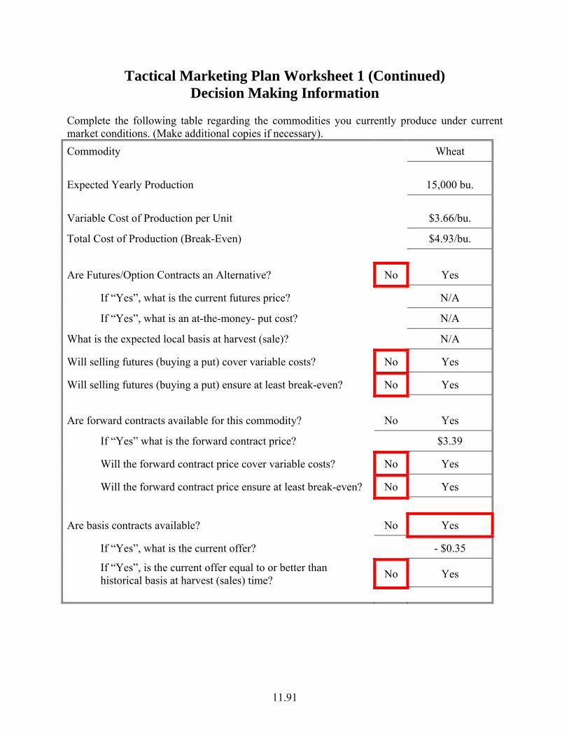
11.91

Tactical Marketing Plan Worksheet 1 (Continued) Decision Making Information

Complete the following table regarding the commodities you currently produce under current market conditions. (Make additional copies if necessary). Commodity Wheat Expected Yearly Production 15,000 bu. Variable Cost of Production per Unit $3.66/bu.

Total Cost of Production (Break-Even) $4.93/bu.








If “Yes” what is the forward contract price? $3.39

Will the forward contract price cover variable costs? No Yes

Will the forward contract price ensure at least break-even? No Yes


If “Yes”, what is the current offer? - $0.35


11.92

Tactical Marketing Plan Worksheet 1 (Continued) Decision Making Information

Complete the following table regarding the commodities you currently produce under current market conditions. (Make additional copies if necessary). Commodity Grain Sorghum Expected Yearly Production 4,200 cwt Variable Cost of Production per Unit $1.56/cwt

Total Cost of Production (Break-Even) $3.89/cwt








If “Yes” what is the forward contract price? $3.30/cwt

Will the forward contract price cover variable costs? Yes

Will the forward contract price ensure at least break-even? No


If “Yes”, what is the current offer? N/A


11.93

Tactical Marketing Plan Worksheet 2 Tactical Decision


Commodity Name Stocker Cattle

Current Month and Year August 2005

Months from Harvest (or sale) 9 Months

General Price Level Top Third Middle Third Bottom Third

Long Term Price Outlook

Short Term Price Outlook

Seasonal Price Trend Outlook

Current Local Basis Top Third Middle Third Bottom Third

A Priori Decision for this situation Price 100% of Expected Production

Decision: Price 100% of expected production of cattle that will be ready in May through the use of forward contracts.

Why? This follows my a priori decision for this situation. Also, another BSE scare could result in a drop in prices.

11.94

Tactical Marketing Plan Worksheet 2 (Continued) Tactical Decision


Commodity Name Wheat








A Priori Decision for this situation Hold Tight and Watch the Market

Decision: Hold Tight and Watch the Market.

Why?

While the short term outlook is down, seasonal price trends suggest a strengthening in prices in the near term. Also, the a priori decision that is being used is for six months away from harvest. We are currently nine months away. I would like to just sit and watch this market for a couple more months and see if prices will follow the seasonal trend. However, if prices do in fact fall $0.15, I will reconsider this decision.

11.95

Tactical Marketing Plan Worksheet 2 (Continued) Tactical Decision


Commodity Name Grain Sorghum








A Priori Decision for this situation N/A

Decision: N/A.

Why? Grain sorghum is a secondary crop. I will do what I have always done. I will harvest the crop and get the best local price I can for the crop.

Documents

DEVELOPING A MARKETING PLAN - …sanangelo.tamu.edu/files/2011/11/K.-Marketing-Plan.pdf · The second step in preparing a marketing plan is to review your ... agronomic and crop rotation