Embed Size (px)
Citation preview
Determining Priority Vegetation Polygons for Common Stand Exam Data
Collection Using a GIS-based Sampling Strategy
By Kristin M. Kolanoski
A Practicum
Submitted in Partial Fulfillment
of the Requirements for the Degree of
Master of Science
in Applied Geospatial Sciences
Department of Geography, Planning, and Recreation
Northern Arizona University
March 8, 2017
Approved by:
Amanda Stan, Ph.D.
Erik Schiefer, Ph.D.
Tony Smith

Determining Priority Vegetation Polygons for Common Stand Exam Data Collection Using a GIS-based Sampling Strategy
i
Acknowledgments
I would like to thank my advisors for giving me guidance during these last several
years while I have been working towards obtaining a Master’s in Applied Geospatial
Sciences from Northern Arizona University. My supervisor Tony Smith also gave me
much needed support and encouragement while I was in school and simultaneously
working fulltime in the GIS shop on the GMUG. The experience of working on this
project was very rewarding for me; it gave me an opportunity to pursue an advanced
degree in GIS while providing a needed deliverable for the GMUG.
I also thank my husband Corey and daughter Sienna for their patience and
understanding of my commitment to completing this degree and Sally Zwisler for her
knowledge and help with understanding all of the components of the regional
change detection project before she retired from the US Forest Service in January,
2016. Furthermore, I appreciate Carol Howe’s continued dedication to this ongoing
project and her coordination and communication with RSAC, GMUG timber staff, and
USFS Region 2 Vegetation Applications Coordinator to encourage forward movement
of and assist with the mortality update process for the GMUG.

Determining Priority Vegetation Polygons for Common Stand Exam Data Collection Using a GIS-based Sampling Strategy
ii
Table of Contents
ACKNOWLEDGMENTS .............................................................................................................................. I
TABLE OF CONTENTS .............................................................................................................................. II
LIST OF TABLES AND FIGURES ................................................................................................................ V
ABSTRACT ............................................................................................................................................... 1
CHAPTER OUTLINE .................................................................................................................................. 4
CHAPTER ONE ......................................................................................................................................... 5
1.1 INTRODUCTION .......................................................................................................................................... 5 1.2 PROBLEM STATEMENT .............................................................................................................................. 11 1.3 PRACTICUM QUESTIONS ........................................................................................................................... 11
CHAPTER TWO ...................................................................................................................................... 13
LITERATURE REVIEW ..................................................................................................................................... 13 2.1 TREE MORTALITY ON GMUG .................................................................................................................... 13 2.2 ARCGIS MODELBUILDER FOR DECISION SUPPORT ...................................................................................... 17 2.3 APPLICATIONS OF REMOTELY SENSED DATA IN US FOREST SERVICE .............................................................. 22 2.4 CHANGE DETECTION FOR FOREST MANAGEMENT ........................................................................................ 24
2.4.1 Use of Spectral Vegetation Indices in Change Detection .............................................................. 25 2.4.2 Change Detection of Tree Mortality ............................................................................................. 30
2.5 REMOTE SENSING APPLICATION FOR MEETING FOREST MANAGEMENT OBJECTIVES ........................................ 31 2.5.1 Use of High Spatial Resolution Satellite Data ............................................................................... 34
CHAPTER THREE .................................................................................................................................... 37
METHODOLOGY ............................................................................................................................................ 37 3.2 TOOLS AND OTHER APPLICATIONS ............................................................................................................. 37 3.3 PROJECT PHASES .................................................................................................................................... 38 3.1 DESCRIPTIONS OF FSVEG AND FSVEG SPATIAL ............................................................................................ 38
3.3.1 Phase I ........................................................................................................................................... 41 Step 1 ................................................................................................................................................................ 42 Step 2 ............................................................................................................................................................... 43 Step 3 ............................................................................................................................................................... 44
3.3.2 Phase II.......................................................................................................................................... 44 Cluster Analysis ................................................................................................................................................ 44 Steps 4 and 5.................................................................................................................................................... 45 Step 6 ............................................................................................................................................................... 46
3.3.3 Phase III ........................................................................................................................................ 50 Tool Creation ................................................................................................................................................... 50 General Overview of Priority Polygon Sampling Tools .................................................................................. 53 Detailed Tool Descriptions .............................................................................................................................. 55
Linked Plot Tool .......................................................................................................................................... 55 Slope Tool ................................................................................................................................................... 59 First Priority Polygon Sampling Criteria ..................................................................................................... 61
Overlaying First Priority Polygons with Vegetation Altering Activities ............................................... 68 Second Priority Polygon Sampling Criteria ................................................................................................ 69 Third Priority Polygon Sampling Criteria .................................................................................................... 72 Final Priority Polygon Tool and VAA Intersection with Priority Polygons ................................................ 74 Review of Final Priority Polygons .............................................................................................................. 75
3.3.4 Phase IV ........................................................................................................................................ 76

Determining Priority Vegetation Polygons for Common Stand Exam Data Collection Using a GIS-based Sampling Strategy
iii
Polygon Redelineation .................................................................................................................................... 76 Plot Layout ....................................................................................................................................................... 78
CHAPTER FOUR ..................................................................................................................................... 82
RESULTS ...................................................................................................................................................... 82 4.1 PHASE I .................................................................................................................................................. 82
4.1.1 Cluster Analysis ............................................................................................................................. 82 4.1.2 Detected Change and Changed Polygons ..................................................................................... 82
4.2 PHASE II ................................................................................................................................................ 86 4.2.1 Priority Strata ............................................................................................................................... 86 4.2.2 Linked Plot Tool Results ............................................................................................................... 86
4.3 PHASE III ............................................................................................................................................... 89 4.3.1 Slope Tool ..................................................................................................................................... 89 4.3.2 Polygon Sampling Tools ............................................................................................................... 90
Overlaying First Priority Polygons with Vegetation Altering Activities ......................................................... 92 Second and Third Priority Polygon Selections ............................................................................................... 92 Determination of Final Priority Polygons ....................................................................................................... 93
Final Priority Polygons with VAAs .............................................................................................................. 93 Final Selection of Priority Polygons ........................................................................................................... 93
4.4 PHASE IV ............................................................................................................................................... 95 4.4.1 Polygon Redelineation .................................................................................................................. 95 4.4.2 Plot Layout and Contract Maps .................................................................................................... 98
CHAPTER FIVE ..................................................................................................................................... 101
DISCUSSION ............................................................................................................................................... 101 5.1 HIGH COMPLEXITY ................................................................................................................................. 101 5.2 COST ................................................................................................................................................... 103 5.3 USE OF NDVI DATA COMPARED TO AERIAL DETECTION SURVEY DATA ........................................................ 105 5.4 FSVEG SPATIAL DISCREPANCIES ............................................................................................................. 106
5.4.1 Polygons In Need of Redelineation ............................................................................................. 106 5.4.2 Inaccurate Species Compositions for Some Polygons ................................................................ 107 5.4.2 Linked and Unlinked Plots .......................................................................................................... 107
5.5 RELATIONSHIP CRITERIA ........................................................................................................................ 108 5.6 CONCLUSIONS ...................................................................................................................................... 109
5.6.1 Future Work ............................................................................................................................... 110 5.6.2 Management Implications ......................................................................................................... 112 5.6.3 Final Remarks ............................................................................................................................. 112
REFERENCES ........................................................................................................................................ 114
APPENDIX A .......................................................................................................................................... A-1
SUPPLEMENTAL LITERATURE REVIEW ................................................................................................ A-1
A.1 US FOREST SERVICE BACKGROUND INFORMATION .................................................................................... A-1 A.1.1 Policy Guiding Land Management Decision Making in the U.S. Forest Service ........................... A-1 A.1.2 Role of Adaptive Management................................................................................................... A-3
A.2 ROLE OF FIELD COLLECTED DATA, AERIAL DETECTION SURVEY DATA, AND REMOTELY SENSED DATA ............. A-9 Supplemental Literature Review References .................................................................................. A-12
APPENDIX B .......................................................................................................................................... B-1
ADDITIONAL FIGURES .................................................................................................................................. B-1 FIGURE B-1. FLOWCHART DETAILING THE STEPS TAKEN TO COMPLETE THE TASKS FOR THE PRACTICUM PROJECT. COMPLEMENT TO FIGURE 4 IN CHAPTER 3. .................................................................................................... B-1 FIGURE B-2. ............................................................................................................................................... B-3

Determining Priority Vegetation Polygons for Common Stand Exam Data Collection Using a GIS-based Sampling Strategy
iv
FIGURE B-3. ............................................................................................................................................... B-4 FIGURE B-4. ............................................................................................................................................... B-5 FIGURE B-5. ............................................................................................................................................... B-6 FIGURE B-6. ............................................................................................................................................... B-7 FIGURE B-7. ............................................................................................................................................... B-8 FIGURE B-8. ............................................................................................................................................... B-9 FIGURE B-9. ............................................................................................................................................. B-10
Determining Priority Vegetation Polygons for Common Stand Exam Data Collection Using a GIS-based Sampling Strategy
v
List of Tables and Figures FIGURE 1. VISUAL EXAMPLES OF NDVI CALCULATION .............................................................................. 26 FIGURE 2. ELECTROMAGNETIC SPECTRUM ................................................................................................ 27 FIGURE 3. FORM USED DURING POLYGON WALKTHROUGHS TO UPDATE EXISTING POLYGON
ATTRIBUTES IN FSVEG SPATIAL ......................................................................................................... 40 IN THE FIRST PHASE OF THE STUDY, I EXAMINED THE DELIVERABLE FROM RSAC THAT CONSISTED OF
A FEATURE CLASS OF VEGETATION POLYGONS ON THE GMUG. ATTRIBUTES OF THE FEATURE CLASS CONSTITUTED OF A FIELD INDICATING PERCENT CHANGE ASSOCIATED WITH EACH POLYGON AND A FIELD INDICATING WHETHER OR NOT A POLYGON NEEDED TO BE CHECKED FOR POSSIBLE SPATIAL REDELINEATION. RSAC BASED THE NEED OF SPATIAL REDELINEATION OF POLYGONS ON TWO FACTORS. THE FIRST FACTOR INVOLVED THE AMOUNT OF CHANGE DETECTED WITHIN EACH POLYGON AND THE SECOND FACTOR CONSIDERED THE ARRANGEMENT OF CHANGE DETECTED ............................................................................................ 42
FIGURE 4. GENERALIZED FLOWCHART DESCRIBING PROJECT PHASES AND STEPS WITHIN EACH PROJECT PHASE. FIGURE B-1 IN APPENDIX B PROVIDES MORE DETAIL FOR PROJECT PHASES AND THEIR STEPS. ............................................................................................................................... 42
FIGURE 5. DEFINITION QUERY FOR VEGETATION ALTERING ACTIVITIES (VAAS) .................................. 48 FIGURE 6. GEODATABASE ORGANIZATION OF THE SIX MODELS PRODUCED TO SELECT PRIORITY
POLYGONS FOR CSE DATA COLLECTION ........................................................................................... 52 TABLE 1. CRITERIA USED IN EACH OF THE THREE PRIORITY POLYGON SAMPLING TOOLS TO SELECT
POLYGONS FOR CSE DATA COLLECTION ........................................................................................... 54 FIGURE 7. LINKED PLOT TOOL AS VIEWED FROM THE MODELBUILDER WINDOW............................... 58 FIGURE 8. LINKED PLOT TOOL AS VIEWED FROM THE TOOL DIALOG BOX ........................................... 58 FIGURE 9. SLOPE TOOL VIEWED FROM THE MODELBUILDER WINDOW ............................................... 60 FIGURE 10. SLOPE TOOL VIEWED FROM THE TOOL DIALOG BOX. ........................................................... 61 FIGURE 11. FIRST PRIORITY POLYGON SAMPLING TOOL AS SEEN FROM THE MODELBUILDER
WINDOW ............................................................................................................................................. 65 FIGURE 12. FIRST PRIORITY POLYGON SAMPLING TOOL AS VIEWED FROM THE TOOL DIALOG BOX .. 66 TABLE 2. ATTRIBUTE FIELDS CALCULATED BY THE FIRST PRIORITY POLYGON SAMPLING TOOL AND
USED BY THE SECOND AND THIRD PRIORITY POLYGON SAMPLING TOOLS FOR SUBSEQUENT SELECTIONS OF PRIORITY POLYGONS. ............................................................................................. 66
FIGURE 13. SECOND PRIORITY POLYGON SAMPLING TOOL AS VIEWED FROM THE MODELBUILDER WINDOW .............................................................................................................................................. 71
TABLE 3. ATTRIBUTE FIELDS AND SQL EXPRESSIONS USED BY SECOND PRIORITY POLYGON SAMPLING TOOL TO SELECT AND DESIGNATE SECOND PRIORITY POLYGONS .............................. 72
FIGURE 14. THIRD PRIORITY POLYGON SAMPLING TOOL AS VIEWED FROM THE MODELBUILDER WINDOW .............................................................................................................................................. 73
TABLE 4. ATTRIBUTES FIELDS AND SQL EXPRESSIONS USED BY THE THIRD PRIORITY POLYGON SAMPLING TOOL TO SELECT AND DESIGNATE THIRD PRIORITY POLYGONS ................................. 74
FIGURE 15. FINAL PRIORITY POLYGON TOOL AS VIEWED FROM THE MODELBUILDER WINDOW ........ 75 FIGURE 16. SYSTEMATIC GRIDS USED FOR PLOT LAYOUT IN STEP 10 OF PHASE IV. ............................... 81 TABLE 5. NUMBER OF ACRES BY STRATA SHOWING DETECTED CHANGE RANGING FROM 1% TO 100%
FROM 1989 UNTIL 2014 WITHIN THE GMUG BOUNDARY. ................................................................83 FIGURE 17. ALL CHANGE (>0% TO 100%) IN NDVI FROM 1989 UNTIL 2014 ON THE GMUG. NDVI CHANGE
IS IN BLUE. .......................................................................................................................................... 84 FIGURE 18. COUNT ACREAGE OF CHANGED POLYGONS BY NINE STRATA ON THE GMUG. ................. 85 TABLE 6. APPROXIMATE COST OF FIELD DATA COLLECTION USING A 10% SAMPLE FOR EACH OF THE 3
PRIORITY STRATA. ............................................................................................................................... 87

Determining Priority Vegetation Polygons for Common Stand Exam Data Collection Using a GIS-based Sampling Strategy
vi
FIGURE 19. BAR GRAPH INDICATING NUMBER OF POSSIBLY VALID LINKED PLOTS TO USE IN BUILDING MORTALITY RULE SETS. ................................................................................................... 89
TABLE 7. NUMBER OF CHANGED POLYGONS MEETING EACH CRITERIA. THOSE NOT MEETING EACH CRITERIA ARE SHOWN IN PARENTHESES WITH TOTALS. ................................................................. 91
FIGURE 20. EXAMPLE OF VAA INTERSECTION WITH PRIORITY POLYGONS WHEREBY VAAS TOUCH THE BOUNDARIES OF THREE PRIORITY POLYGONS AND HAVE ONLY AFFECTED A MINUTE PERCENTAGE OF THE POLYGONS’ AREA. .......................................................................................... 92
TABLE 8. ACREAGE AND NUMBER OF FINAL PRIORITY POLYGONS BY STRATA DESCRIPTION AND BY RANGER DISTRICT. THE NUMBER OF POLYGONS FLAGGED BY RSAC AS NEEDING TO BE CHECKED FOR REDELINEATION AND THE PERCENTAGE OF STRATA ACREAGE REPRESENTED BY PRIORITY POLYGONS ARE ALSO INCLUDED...................................................................................................... 94
FIGURE 21. SLIGHT MODIFICATION IN POLYGON BOUNDARY CONSIDERED AS A REDELINEATION. YELLOW LINE INDICATES REDELINEATED BOUNDARY AND BLACK LINE REPRESENTS OLD POLYGON BOUNDARY. ...................................................................................................................... 95
FIGURE 22. RESULT OF SPLITTING A LARGE POLYGON (IN BLACK) INTO SEVERAL SMALLER POLYGONS (IN YELLOW). THIS IMAGE SHOWS A SPLIT OF ONE LODGEPOLE PINE MIX POLYGON INTO THREE SEPARATE POLYGONS. YELLOW LINE DESIGNATES NEW POLYGON DELINEATIONS AND BLACK LINE DISPLAYS OLD POLYGON BOUNDARIES. ...................................................................... 97
TABLE 9. PRIORITY POLYGONS ON GUNNISON RD REDELINEATED BY SILVICULTURIST ..................... 98 FIGURE 23. EXAMPLE OF OVERVIEW MAP FOR PRIORITY POLYGONS INCLUDED IN CSE DATA
COLLECTION CONTRACT (1 OF 9 MAPS). THE RED BOX IN THE INSET MAP SHOWS THE EXTENT OF THE MAIN MAP AND THE LOCATION ON THE GMUG OF THE POLYGONS DISPLAYED WITHIN THE MAP. ............................................................................................................................................ 99
FIGURE 24. EXAMPLE OF A DATA DRIVEN MAP FOR CSE DATA COLLECTION CONTRACT. EACH MAP SHOWS ONE POLYGON. FOR THIS REASON, THERE ARE 462 MAPS INCLUDED IN THE CONTRACT. ............................................................................................................................................................ 100
FIGURE B-2. MAP A OF FINAL PRIORITY POLYGON VICINITY MAP COLLECTION (2 OF 9) ..................... B-3 FIGURE B-3. MAP B OF FINAL PRIORITY POLYGON VICINITY MAP COLLECTION (3 OF 9) ..................... B-4 FIGURE B-4. MAP C OF FINAL PRIORITY POLYGON VICINITY MAP COLLECTION (4 OF 9) ..................... B-5 FIGURE B-5. MAP D OF FINAL PRIORITY POLYGON VICINITY MAP COLLECTION (5 OF 9) ..................... B-6 FIGURE B-6. MAP F OF FINAL PRIORITY POLYGON VICINITY MAP COLLECTION (6 OF 9) ..................... B-7 FIGURE B-7. MAP G OF FINAL PRIORITY POLYGON VICINITY MAP COLLECTION (7 OF 9) ..................... B-8 FIGURE B-8. MAP H OF FINAL PRIORITY POLYGON VICINITY MAP COLLECTION (8 OF 9) .................... B-9 FIGURE B-9. MAP I OF FINAL PRIORITY POLYGON VICINITY MAP COLLECTION (9 OF 9) ..................... B-10
Determining Priority Vegetation Polygons for Common Stand Exam Data Collection Using a GIS-based Sampling Strategy
1
ABSTRACT
Forests in the western United States have experienced high levels of tree mortality
over the last ten to fifteen years. Climate change has been touted as a major cause
of this mortality. Climate change is associated with an increase or change in biotic
and abiotic agents that serve as environmental stressors to ecosystem function and
structure, testing the ability of certain tree species to respond and survive in
environmental conditions outside of historic variability. Bark beetle infestations and
factors associated with sudden aspen decline (SAD) are examples of these
environmental stressors linked to the unprecedented mortality in spruce (Picea spp.),
fir ( Abies spp.), pine (Pinus spp.), and aspen (Populus tremuloides) stands across the
western US. The Grand Mesa, Uncompahgre, and Gunnison National Forests (GMUG)
in southwestern Colorado have not been excluded from this tree mortality
phenomenon. Over 229,000 acres of aspen and 223,000 acres of spruce have been
negatively affected by SAD and spruce beetle, respectively on these three Forests
over the last decade. Unfortunately, in addition to the negative effects these
occurrences have had on the health of these forested ecosystems, the
unprecedented tree mortality has also led to inaccurate measurements of stand
condition in US Forest Service (USFS) databases for the GMUG. More specifically,
tree mortality has altered percentages of live and dead trees and corresponding
canopy cover estimations within forested polygons. Accurate characterizations of
existing vegetation structure are needed to plan treatments aimed at building

Determining Priority Vegetation Polygons for Common Stand Exam Data Collection Using a GIS-based Sampling Strategy
2
resilience and recovery of spruce and aspen on the Forests as well as to fulfill the
need of the planning framework for the revision process of GMUG’s Land and
Resource Management Plan, which is slated to begin in 2017. Vegetation polygons
that are created and maintained in a USFS geodatabase system, known as FSVeg
Spatial, are the units that delineate and describe existing vegetation on the GMUG
and other National Forests and Grasslands. According to the R2 Supplement of the
FSVeg Spatial User Guide, individual polygons are generally homogeneous in
dominant lifeform, species composition, percent crown cover, size, vertical and
horizontal structure, and tree crown condition. Recorded attributes of polygons
include species, tree size class, crown condition, and canopy cover percentage,
including the percentage of the canopy that is dead. Remotely sensed data has been
used by the Remote Sensing Applications Center (RSAC) to detect significant change
that has occurred from 1989 until 2014 in these polygons caused by tree mortality.
Because there are over 18,000 forested polygons on the three Forests that have
experienced significant tree mortality, an automated algorithm will be created to
update live and dead canopy cover percentages of each polygon included in the
update procedure. Before the employment of this update, field data at the polygon
level needs to be collected in order to calculate tree mortality rates by species and
size class and build tree mortality rule sets for use in the algorithm. To choose
polygons for field data collection, or common stand exam (CSE) data collection, a

Determining Priority Vegetation Polygons for Common Stand Exam Data Collection Using a GIS-based Sampling Strategy
3
GIS-based sampling strategy was developed and documented using ArcGIS
ModelBuilder (v. 10.3.1). Some of the considerations in building the sampling strategy
were as follows: the strata to which a polygon belonged, proximity of a polygon to
maintained roads, a polygon’s location in regards to Wilderness or areas with special
protection designations, a polygon’s size, the date at which CSE data collection
occurred if CSE data had been collected in a polygon in previous years, whether or
not reshaping of a polygon in its current state was needed to meet the definition of a
polygon outlined in the R2 Supplement to the FSVeg Spatial User Guide, and the
funds allocated to CSE data collection. The purpose of this Practicum was to
prioritize and select forested vegetation polygons for CSE data collection using a GIS-
based sampling strategy. The polygon prioritization resulting from the sampling
strategy would then provide guidance of where to focus CSE data collection efforts
on the GMUG for the mortality update project (also known as the change detection
project) while trying to minimize the cost of contract data collection.

Determining Priority Vegetation Polygons for Common Stand Exam Data Collection Using a GIS-based Sampling Strategy
4
Chapter Outline This Practicum document consists of five chapters. Chapter 1 provides an
introduction, leading to the problem statement, project questions, and purpose of
the project. Chapter 2 consists of a literature review of areas of research applicable
to the vegetation polygon update process discussed in this Practicum. Chapter 3
details the methods used to conduct the GIS work needed to answer the questions
raised in Chapter 1. Chapter 4 presents the results of the GIS work. Chapter 5
discusses the results arising from the GIS work conducted and gives conclusions
drawn from the results. Chapter 5 also provides the reader with an understanding of
any problems, issues, and difficulties encountered while completing tasks outlined in
the methodology section. Chapter 5 also provides a discussion on management
implications of the work completed in this project and how the data used in this
project will continue to be used in improving characterizations of forested vegetation
polygons on the GMUG. The appendices provide additional literature review and
supplemental figures related to the Practicum project.

Determining Priority Vegetation Polygons for Common Stand Exam Data Collection Using a GIS-based Sampling Strategy
5
Chapter One
1.1 Introduction Forest stands across the western United States and Canada have experienced a
dramatic increase in tree mortality over the last ten to fifteen years (Mueller et al.
2005; Marchetti et al. 2011; Bentz et al. 2010; Michaelian et al. 2011; Anderegg et al.
2013; USDA Forest Service, 2016a). Drought and elevated temperatures have caused
trees to be physically stressed and in turn, more vulnerable to insect and disease
infestations and attacks (Herbertson and Jenkins, 2008; Bentz et al. 2010). Trees
unable to protect themselves from insect and disease attacks due to their weakened
defense mechanisms eventually die. The result is a large number of trees within
stands dying, a process that initiates significant changes in structure, composition,
and function of stands and overall decreased forest health.
Silviculture has been a long standing practice, since the early 20th century in America,
by which various treatments often including some kind of tree removal technique(s)
are applied to create and manage forest stands according to the purpose and
objectives established by the governing agency or landowner (Mustian, 1978, Smith
et al. 1997). Classifying stands prior to designing treatments is essential for
successful implementation of the treatments and accomplishing the desired
objectives. Multiple methods have been utilized to characterize forest stands. The
methods can involve one or more of the following: field reconnaissance and
observations by a silviculturist or forester, detailed vegetation composition data

Determining Priority Vegetation Polygons for Common Stand Exam Data Collection Using a GIS-based Sampling Strategy
6
using field plots such as with common stand exams (CSE), remote sensing data, and
more recently LiDAR data (Moffiet et al. 2005; McRoberts et al. 2010; Pascual et al.
2013; Kelley and Di Tommaso 2015). In general, stand classification involves
determining general differences in composition and structure of the forest across a
landscape, establishing stand boundaries to spatially designate different stands
according to these general differences, and then determining tree species, age class
(by measuring height and diameter at breast height), basal area, and canopy cover or
crown closure, and other related attributes within each of the stands.
The GMUG in southwestern Colorado has experienced an increase in tree mortality,
especially in stands consisting of Engelmann spruce (Picea engelmannii), subalpine fir
(Abies lasiocarpa), Douglas-fir (Pseudotsuga menziesii), white fir (Abies concolor), and
aspen (Populus tremuloides) over the last ten to fifteen years (Marchetti et al. 2011;
Worall et al. 2010; USDA Forest Service, 2016a). Climate change has been linked to
the increase in bark beetle infestation, sudden aspen decline, and other diseases and
insect infestations causing the unprecedented tree mortality on the GMUG (Worall et
al. 2008; Worall et al. 2010; Marchetti et al. 2011; Rehfeldt et. al 2015; USDA Forest
Service, 2016a). Other damage causal agents such as western spruce budworm
(Choristoneura occidentalis) and fir engraver (Scolytus ventralis) are also contributing
to the mortality of spruce and fir on the Forests (Todd Gardiner, personal
communication, April 25, 2015). To attempt to address this increase in tree mortality

Determining Priority Vegetation Polygons for Common Stand Exam Data Collection Using a GIS-based Sampling Strategy
7
and decrease in forest health, the GMUG is in the process of implementing
silvicultural treatments under the direction of the Spruce Beetle Epidemic Aspen
Decline Management Response (SBEADMR) project. A Record of Decision (ROD) for
the Environmental Impact Statement (EIS) for SBEADMR was issued and signed by
GMUG’s Forest Supervisor in July, 2016. This project has and will implement different
silvicultural and fuels management treatments across the GMUG, focusing on the
promotion of resiliency and recovery within stands consisting of Picea engelmannii
(Engelmann spruce) and Populus tremuloides (aspen) (USDA Forest Service, 2016a).
Planning for this project was programmatic in nature, which means the project was
designed so that treatments could be implemented once the necessary surveys and
clearances are made and not prior to the ROD of the EIS being signed. Therefore, no
comprehensive stand exam data or forest inventory took place specifically for
planning of SBEADMR prior to it being approved. In many areas on the GMUG, stand
attributes were populated using the original aerial photography interpretation, much
of it occurring in late 1980s and early 1990s, to delineate and describe vegetation
polygons. Therefore, the tabular records of many forested vegetation polygons are
in need of being updated to represent existing conditions on the GMUG for use in the
SBEADMR project.
A vegetation polygon is defined by the R2 Supplement to the FSVeg Spatial User
Guide as an area being generally homogeneous in structure and composition. More

Determining Priority Vegetation Polygons for Common Stand Exam Data Collection Using a GIS-based Sampling Strategy
8
specifically, a polygon needs to be similar and uniform in dominant lifeform, species
composition, percent crown cover, size, vertical and horizontal structure, tree crown
condition, and occasionally topographic features that may be indicative of vegetative
change such slope breaks (USDA Forest Service, 2016b). Some polygons can be void
of vegetation and are identified by their ground surface cover type such as rock
slides, quarries, glaciers, and wide roads. A forested vegetation polygon is one
having at least 25% of its area consisting of trees (USDA Forest Service, 2016b).
Forested polygons are the focus in this study and whose attributes are to be updated
with the automated algorithm.
Review of stand attributes and spatial delineations of vegetation polygons are
intended to take place prior to determining plot locations for CSE data collection as
well as before any implementation of timber sales and other silvicultural treatments.
If it is determined that edits need to be made to polygons, these edits need to take
place within FSVeg Spatial database prior to plot layout. Stand attributes can be
updated prior to or after CSE data has been collected. Areas can be re-delineated
and reattributed using a variety of different methods, ranging from: 1) field collection
of common stand exam (CSE) point data; 2) interpretation of high resolution aerial
imagery, which provides a moderately accurate approach to classify stands,
depending on the spatial resolution of the data used and interpreted; 3) LiDAR data,
which provides high accuracy in determining stand structure characteristics but not

Determining Priority Vegetation Polygons for Common Stand Exam Data Collection Using a GIS-based Sampling Strategy
9
species composition; and 4) site and stand visits by a silviculturist or forester to
perform qualitative assessments on stands, which provides less accuracy but
potentially more overall species composition and structure information for
characterizing stands. The qualitative assessment involves collecting descriptive
rather than quantifiable information regarding the composition and structure of a
polygon. This assessment is performed using specific agency protocols found within
the R2 Supplement of the FSVeg User Guide. These protocols and the FSVeg Spatial
database is explained further in the Methods section of this document. Nonetheless,
priority of data collection is designated usually for stands where timber sales will
occur in the near future. Other stands in which treatment implementation is not
planned to occur within the next five years usually do not have recently collected
field data associated with them, unless they have been or were supposed to have
been part of a timber sale sometime in the recent past. Therefore, valid field data is
lacking to adequately characterize and update outdated tabular data for forested
vegetation polygons on the GMUG, especially for forested polygons having timber
that is considered unsuitable for potential timber sale.
Additionally, GMUG foresters have not been able to keep up with the need to
implement several treatments over a large number of acres because such large
increases in tree mortality have happened in a short amount of time. Also,
decreasing annual budgets and correspondingly smaller workforces have contributed

Determining Priority Vegetation Polygons for Common Stand Exam Data Collection Using a GIS-based Sampling Strategy
10
to the challenge of meeting the need for increased data collection and performance
and completion of other duties associated with implementing timber sales. These
challenges come at a time when Forest Plan Revision is scheduled to begin in 2017.
Forest Plan Revision will need to rely on existing data for the different resources to
perform assessments, many of which will involve GIS exercises to determine need for
change and revise current management direction and guidelines to be instituted in
the new Forest Plan. Knowledge of existing vegetation conditions are needed to
ascertain desired future conditions of the different resources on the Forests,
including the forested vegetation. Currently, different methods are being looked at
to more quickly update and determine existing vegetation conditions. One such
method is using remotely sensed data to detect significant change within forested
vegetation polygons due to tree mortality and document that change with a spatial
and tabular data update process.
To apply such technologies to update forested polygons on the GMUG and other
Forests in Region 2, methods used in a pilot study conducted from 2011 to 2014 on
225,000 acres of the Parks Ranger District, Medicine Bow-Routt National Forest in
north-central Colorado are being used (Stam et al. 2015a, Stam et. al. 2015b, Stam et
al. 2015c). Region 2 is one of nine broad geographic areas managed by the US Forest
Service and includes National Forests and Grasslands within Colorado, South Dakota,
Nebraska, Kansas, and most of Wyoming. The main impetus for developing this

Determining Priority Vegetation Polygons for Common Stand Exam Data Collection Using a GIS-based Sampling Strategy
11
methodology was to address the changes in vegetation polygons due to increased
tree mortality from bark beetle and other insect and disease infestations across
National Forest lands in Region 2. In the last two years, the Rio Grande and San Juan
National Forests in Colorado have also completed the automated update process for
their forested polygons. On the Rio Grande, 2,680 plots were visited during the 2014
and 2015 field seasons and CSE data was collected from a total of 335 polygons for
the tree mortality update process (Stam et al. 2016). No official report detailing the
update process for the San Juan NF has been released as of yet.
1.2 Problem Statement The purpose of this study was to determine the number and location of polygons
that were visited in the field during the summer of 2016 and will be visited during the
2017 summer field season for CSE data collection. The purpose of collecting CSE data
is to build tree mortality rule sets. Once built, the rule sets will be implemented in an
automated algorithm originally developed in the pilot study conducted on the
Medicine Bow- Routt NF (Stam et al. 2015a, Stam et al. 2015b, Stam et al. 2015c).
However, the algorithm will be customized with tree mortality rule sets specific to
the GMUG when it is used to update live and dead canopy cover percentages of
forested polygons.
1.3 Practicum Questions My research questions addressed in this Practicum included:

Determining Priority Vegetation Polygons for Common Stand Exam Data Collection Using a GIS-based Sampling Strategy
12
1) How many polygons would be included in the base population for sampling
priority polygons?
2) Which strata would be considered for CSE data collection for mortality rate
calculation?
3) How many acres of each stratum need to be sampled to accurately portray
stand conditions in each stratum for CSE data collection? The goal for CSE
data collection for this project was to collect data from 10% of each priority
stratum’s acreage. Then the question follows. If the 10% goal cannot be
attained, then from how many acres in each stratum would data be collected?
4) What and how many criteria would be used in the GIS sampling strategy to
prioritize the polygons to be visited in the field for CSE data collection?
5) How many priority polygons would result from the GIS sampling strategy?
Other more specific questions that were asked in this project included:
6) How many vegetation polygons already had recent and valid CSE plot data
associated with them that reflected existing conditions within the polygons?
7) How many acres of each stratum were covered with recent and valid CSE data
collection?
The Methods section describes the procedures by which these questions were
addressed.

Determining Priority Vegetation Polygons for Common Stand Exam Data Collection Using a GIS-based Sampling Strategy
13
Chapter Two
Literature Review
2.1 Tree Mortality on GMUG Forests in the Rocky Mountain region or Region 2, and especially on the GMUG, have
experienced a large amount of tree mortality due to the infestation of bark beetles
(Dendroctonus spp., Scolytus ventralis, and Ips spp.). By 2014, approximately 30% of
the total spruce-fir vegetation (223,000 acres) on the GMUG had been damaged by
bark beetle infestation, indicating a rapidly expanding outbreak on the three Forests
(USDA Forest Service, 2016a). Based on projected warming and population models,
Bentz et al. 201o found that thermal regimes conducive to population success of
spruce bark beetle and mountain pine beetle will generally increase throughout this
century even though there are patterns of high spatiotemporal variability for these
regimes. Also, population models suggest that movement of bark beetle populations
to higher latitudes and elevations will occur as a response to increasing temperatures
associated with climate change. Despite the complex nature of bark beetle
interactions with biotic and abiotic factors and the uncertainty associated with
predicting the insects’ responses to climate change, many view the decline of spruce
as a response to climate change as inevitable (Bentz et al. 2010).
Modeling has been shown to be a useful tool in showing changes in population
distributions over time and climatic niches, those range of climatic conditions in
which forest tree species are adapted, in response to changing environmental

Determining Priority Vegetation Polygons for Common Stand Exam Data Collection Using a GIS-based Sampling Strategy
14
conditions. Specifically modeling has been used to show areas where spruce will
have the highest likelihood of adapting to and surviving in the next 45 years on the
GMUG (Rehfeldt et al. 2015). The modeling results suggest that land managers
should focus treatment efforts on spruce stands that have a better chance of survival
from climate change effects. Treatments, such as those resulting in basal area
reductions, should be designed to promote conditions within spruce stands that are
more resilient to insect infestations associated with climate change. Hansen et al.
2010 examined stands consisting predominantly of Engelmann spruce that were
treated with partial cutting as a part of forest management activities on the Apache-
Sitgreaves National Forest in Arizona, Medicine Bow-Routt National Forests in
Colorado and Wyoming, and Dixie-Fishlake and Uinta National Forests in Utah. The
purpose of this examination was to evaluate partial cutting as a preventative strategy
of reducing spruce-beetle caused mortality. Hansen et al. 2010 found that despite the
lack of experimental control for factors such as treatment type and random
assignment to experimental units, partial cutting in the central and southern Rocky
Mountain spruce type resulted in significant reductions in subsequent spruce beetle-
caused tree mortality. The GMUG has incorporated resiliency treatments within the
proposed alternatives of the SBEADMR project in order to address the spruce beetle
epidemic that the Forests are currently experiencing and how to plan for the long
term effects of current and future climate change on spruce-fir forests on the GMUG.

Determining Priority Vegetation Polygons for Common Stand Exam Data Collection Using a GIS-based Sampling Strategy
15
In addition to resiliency treatments, sanitation and salvage treatments also are being
utilized in this project to increase the likelihood of stands currently infected being
able to naturally regenerate and recover from spruce beetle attack over time.
Sudden aspen decline (SAD) has led to increased mortality within aspen stands in the
western United States. On the GMUG, SAD was first detected in 2004 and has been
shown to have affected approximately 31% (over 229,000 acres) of aspen on the
GMUG from 2004 to 2010 (USDA Forest Service, 2016a). Sudden aspen decline has
not been contributed to the infestation and attack of an aggressive primary
pathogen(s) or insect(s) but to the rapid, synchronous branch dieback, crown
thinning and mortality of aspen stems on a landscape scale (Worrall et al. 2010).
Stands most effected by or predisposed to the effects of SAD are those existing in
vegetation transition zones or within the lower elevational gradient of aspen that
experience the driest and warmest conditions during periods of drought (Worrall et
al. 2008, Worrall et al. 2010). Furthermore, declining and damaged stands from SAD
were more prone to the negative effects of secondary insects and diseases as
compared to healthy stands to these same agents (Marchetti et al. 2011). These
secondary agents amplified the impact of SAD on trees that died but may have
otherwise recovered from SAD. Furthermore, Ireland et al. 2014 found that mortality
of younger aspen trees was attributed to lower recent growth rates and higher
frequencies of abrupt growth declines and this correlation occurred regardless of the

Determining Priority Vegetation Polygons for Common Stand Exam Data Collection Using a GIS-based Sampling Strategy
16
presence of SAD. This suggests that aspen stands affected by SAD and consisting of
individuals with slower growth rates may not recover as quickly or at all from SAD as
compared to stands consisting of individuals with higher growth rates. Therefore,
recovery of aspen stands from the effects of climate change and SAD will rely on the
species ability to adapt to these abiotic and biotic stressors and how quickly this
adaptation of those stands takes place.
Planning for shifts in vegetative communities over time as a result of climate change
will become a major challenge to land management agencies to address in future
NEPA (National Environmental Policy Act) analyses. In the SBEADMR EIS, the GMUG
has described management actions and treatments that can be implemented over
the three Forests to address the potential changes in spruce-fir and aspen
communities resulting from climate change. More specifically, the SBEADMR project
proposes treatments within opportunity areas consisting of aspen that encourage
aspen regeneration through thinning, prescribed fire treatments, or a combination of
both. However, more research will need to be conducted and further knowledge
gained through adaptive management practices to highlight the importance of which
forest management practices are successful in equipping stands with the ability to be
resilient and respond to the effects of climate change. Perhaps the precepts of
forest health and sustainability will be redefined as forests are built to be more
resilient to changing climatic conditions.

Determining Priority Vegetation Polygons for Common Stand Exam Data Collection Using a GIS-based Sampling Strategy
17
To better design silvicultural treatments for project planning and establish relevant
and SMART (specific, measurable, assignable, realistic, and time-related) objectives in
the revised Forest Plan for the GMUG, recent tree mortality will be accounted for in
forested polygons on the GMUG by using remotely sensed data to detect significant
change within forested polygons and collecting field data to determine percentage
of dead within different strata of polygons. The percentage of dead for each age and
species class within sampled polygons will be quantified by CSE data previously
collected and still valid to use for this purpose. Validity of field data is based on
criteria that is explained in detail in the Methods section. Percentage of mortality will
also be calculated using CSE data collected in the summer of 2016 and additional CSE
data to be collected in the summer of 2017. To select those polygons from which
field data would be collected, while keeping within budget constraints of the project
and addressing the future needs of GMUG timber shops for CSE data collection, I
created a GIS sampling strategy using ArcGIS ModelBuilder. Chapter 3 provides
detail for the formulation of the GIS sampling strategy. Below I provide a literature
review discussing applications of ModelBuilder for natural resources management
along with ways in which remotely sensed data has been employed in directing forest
management practices and policy.
2.2 ArcGIS ModelBuilder for Decision Support The development and technological advances in geographic information systems
(GIS) have been instrumental in advocating efficiency in the way in which resource
specialists, researchers, managers, and educators analyze and decipher relationships,
Determining Priority Vegetation Polygons for Common Stand Exam Data Collection Using a GIS-based Sampling Strategy
18
patterns, and trends among components coexisting on the Earth. GIS has allowed
humans to visually see how these various components interact, are associated with
one another spatially, and how these components change or differ over time within a
spatial context.
The Environmental Systems Research Institute (ESRI) has made it easier for
individuals to operate a GIS and view and analyze the relationships via a computer,
tablet, personal display assistant (PDA), or smartphone device through ArcGIS
software products and ArcGIS Online (AGOL), online GIS. One of the most commonly
and frequently used ArcGIS products is ArcGIS for Desktop which can be operated
from a desktop computer allowing the user to perform data building and editing,
spatial analysis and geoprocessing, modeling, and map display.
One of the most powerful applications that ArcGIS offers is ModelBuilder. It has
been often utilized as a tool to provide direction in decision making for various
resource areas. For this reason, the workflows organized and executed by models
created by programming languages and applications such as ModelBuilder have been
coined as Spatial Decision Support Systems (SDSS) or DSS (Decision Support
Systems). SDSS are models that incorporate both GIS and nonspatial parameters into
the decision making process; however, the term DDS has also been employed in the
literature to describe decision support models utilizing both spatial and nonspatial
parameters. The uses of ModelBuilder have ranged from the development of a DDS
Determining Priority Vegetation Polygons for Common Stand Exam Data Collection Using a GIS-based Sampling Strategy
19
for delineating homogenous regions based on multiple criteria such as hydrography,
physical environment, socioeconomics, and political-administrative aspects for
integrated water resources planning and management (Coelho et al. 2012) to the
creation of a SDDS to support the timber harvesting decision making process in
Austria by comparing harvesting systems and selecting the best suitable system
based both on stakeholder interests and environmental conditions (Kühmaier and
Stampfer 2010). Systems such as these were designed to be flexible and adaptable
and provide some objectivity through the creation of a systematic framework that
structures a decision problem and identifies creative decision alternatives.
ModelBuilder offers many advantages in its use for data analysis involving
geoprocessing and examination of spatial relationships. One main advantage is that
it allows the user to integrate multiple geoprocessing functions into a single
workflow (ESRI, 2016, Allen 2011). Tang et al. 2014 used ModelBuilder along with
ArcHydro Tools to develop a protocol for delineating watershed boundaries in the
Rainwater Basin in south-central Nebraska. This protocol involved processing many
different LiDAR datasets through the execution of a multitude of geoprocessing
functions. Tang et al. 2014 was able to rerun the model to perform the same
geoprocessing functions for each of the different datasets. The end product was
defining playa wetland topographic conditions in the Basin.
Determining Priority Vegetation Polygons for Common Stand Exam Data Collection Using a GIS-based Sampling Strategy
20
Another benefit of ModelBuilder is that it requires no special programming skills of
the user, allowing the user to learn relatively easily and quickly how to build, edit, and
manage models (Tang et al. 2014). Chi (2010) used the interface of ModelBuilder to
generate an index of land developability that could be included in social demographic
research. The hope stemming from this work was to encourage demographers who
lack experience in performing spatial analysis of land use and development in relation
to population research to do just this by having access to an easy to use GIS function
such as the land developability index model. Chi 2010 emphasized that ModelBuilder
shows the procedure of the entire analysis via flowchart which helps demographers
who do not use GIS frequently understand and conduct the model with ease.
Other advantages of ModelBuilder are that it enables the user to document analysis
workflows for projects, rerun the same workflow, and modify an existing model by
changing input datasets or functions for alternative analyses. The USFS and Bureau
of Land Management (BLM) have used ModelBuilder to more easily document
geoprocessing steps of geospatial analyses designed to meet planning needs. Dave
Sinton, GIS Specialist for the BLM Uncompahgre Field Office in Montrose, Colorado,
established official geospatial layers for the alternatives in the BLM Uncompahgre
Resource Management Plan (RMP), currently being revised, using ModelBuilder. The
RMP is the BLM equivalent to the Forest Plan or FLMP for the USFS and is an official
NEPA document. These models established not only the layers but also the

Determining Priority Vegetation Polygons for Common Stand Exam Data Collection Using a GIS-based Sampling Strategy
21
documentation on how the layers were created. One example is the target shooting
additions model in the recreation toolset (Figure 1). This model produced potential
sites for target shooting on BLM lands managed by the Uncompahgre Field Office.
Mr. Sinton also helped the BLM’s State Planner address and answer questions about
RMP alternatives dealing with mineral extraction. He created a model known as the
TL Calculator whose purpose was to calculate the number of acres having timing
limitations and no surface occupancy for mineral extraction on all land administered
by the Uncompahgre Field Office and specifically in the North Fork area. This model
aided in further developing alternatives addressing mineral extraction issues and
concerns.
The USFS has used ModelBuilder in a similar fashion as the BLM in assisting with
planning efforts. For example, the Rio Grande National Forest (RGNF) in Colorado
has used ModelBuilder in creating a layer that displays those RGNF lands that are or
may be suitable for timber production. Cheryl O’Brien, GIS Coordinator for the RGNF,
created this layer as part of the Forest Plan Revision process. Areas having soils with
high mass movement potential, not owned by the USFS, within Wilderness, Colorado
Roadless areas (CRAs), and other specially designated USFS lands, and consisting of
nonindustrial species such as limber pine, bristlecone pine, pinyon, and juniper were
the criteria used in the model to represent those lands unsuitable for timber
production (Rebain, 2016).

Determining Priority Vegetation Polygons for Common Stand Exam Data Collection Using a GIS-based Sampling Strategy
22
A second example in which ModelBuilder has been used by the USFS is to provide
information support in the area of travel management. In 2015, I produced four
models in Modelbuilder that worked together to produce a road layer for the GMUG
that represented the minimum road set regulated in Subpart A of the Travel
Management Rule (TMR). TMR (Code of Federal Regulations, 2015a, Code of Federal
Regulations, 2015b, Code of Federal Regulations, 2015c) directs National Forests to
balance the use of the Forests by off road vehicles (ORVs) with other uses of the
Forests that may be incompatible with ORV use and with the environmental integrity
of the Forests. Subpart A specifically directs the Forest Service to identify the most
ecologically, economically, and socially sustainable road system in terms of access for
recreation, research, and other land management activities. The created models
assisted with meeting the requirements outlined in Subpart A by identifying those
roads under GMUG jurisdiction that are needed to administer NFS lands and are not
posing high risks to water resources and wildlife. In all, Modelbuilder meets two
critical needs of land management agencies for project and FLMP or RMP planning,
efficient execution of elaborate geospatial analyses and essential workflow
documentation for project records.
2.3 Applications of Remotely Sensed Data in US Forest Service Remote sensing data has been used in different applications and analyses to view the
Earth for several decades, particularly since the launch of the first of the Landsat
satellites in 1972 (Cohen and Goward 2004). One of most applied uses of remotely

Determining Priority Vegetation Polygons for Common Stand Exam Data Collection Using a GIS-based Sampling Strategy
23
sensed data has been to detect change in land cover and land use (LCLU) over time
(Kennedy et al. 2007, Knorn et al. 2009, Xian et al. 2009, Andrew et al. 2014). In
addition to detecting change in LCLU on USFS lands, the US Forest Service has
utilized remote sensing data to view the state and condition of natural resources
over the landscape and determine the changes in resource condition over time.
Moreover, the agency has applied these remote sensing technologies in directing
natural resource management and policy on USFS lands.
Remotely sensed data has supported the implementation and enforcement of the
TMR. The use of 1 m IKONOS satellite images overlaid on GIS maps of USFS system
roads helped monitor and identify unofficial, nonsystem roads and trails created by
ORV recreational use and pinpoint hotspot areas where the density of unofficial and
nonsystem trails was highest on the Dixie National Forest in Utah and Bridger-Teton
National Forest in Wyoming (Mayer and Lopez 2011).
For approximately twenty years, the Remote Sensing Applications Center (RSAC) of
the USFS, now the Geospatial Technology Applications Center (GTAC) , has helped
agency field units develop and implementless costly ways to obtain needed forest
resource information. It has conducted multiple projects utilizing and analyzing
remote sensing data to provide assistance in the areas of resource inventory, fire and
fuels, land cover change, and forest health among many others. For example, RSAC
recently examined whether Landsat data could be used to assess and monitor aspen

Determining Priority Vegetation Polygons for Common Stand Exam Data Collection Using a GIS-based Sampling Strategy
24
defoliation from aspen leaf miner in Alaska (Biswas et al. 2016). In addition, RSAC
generated LiDAR-derived 3-D canopy structure derivatives for describing canopy
height and density across the Kaibab Plateau,producing LiDAR forest inventory
models for modeling field-derived forest inventory parameters (Mitchell et al. 2015).
RSAC plans to use these models to help understand the links between 3-D canopy
structure and goshawk demographic performance on the Plateau. These projects,
among many others, have produced improved resource information for agency field
units or, in some cases, supplied first time data that has been invaluable in guiding
resource management planning efforts and has assisted USFS resource specialists
and land managers in making better informed resource management decisions.
2.4 Change Detection for Forest Management
One of the most well-known applications of remote sensing is change detection. The
premise in using remotely sensed data for change detection is that real changes in
objects of interest will be detected based on changes in reflectance values or local
textures rather than changes caused by other factors such as differences in
atmospheric conditions, illumination and viewing angles, and soil moistures (Deng et
al. 2008). Change detection requires the analysis of multitemporal imagery in which
images are acquired at two different times or over a continuous time scale or time
trajectory, to show a change in some aspect of ecosystem condition and/or function
over time (Singh 1989, Coppin et al. 2004). This type of analysis can provide useful
information for land management planning and decision making at local, regional,

Determining Priority Vegetation Polygons for Common Stand Exam Data Collection Using a GIS-based Sampling Strategy
25
national, and global levels (Deng et al. 2008). Changes on the landscape can occur
either due to anthropogenic causes or due to natural disturbance events. Also, the
rate of change can either be abrupt such as change caused by wildfire, logging
activities, or landslides or more gradual such as change from development or
biomass accumulation, allowing change to be assessed as either a categorical or
continuous variable (Coppin et al. 2004). Change detection techniques using
remotely sensed data involve procedures for both change extraction and change
separation and labelling, with one method potentially yielding a significantly
different change map than an alternate method. These techniques will not be
discussed in detail in this paper; however, many can be reviewed in Coppin et al.
2004, Collins and Woodcock 1996, and Singh 1989. Additionally, more simplistic
explanations of many of the change detection techniques can be found in Campbell
and Wynne 2011 and Lillesand et al. 2015.
2.4.1 Use of Spectral Vegetation Indices in Change Detection Spectral vegetation indices (SVIs) have been instrumental in detecting and extracting
change in vegetation condition both within an image and among image sets. The
purpose of a SVI is to combine the effects of several spectral bands into a single value
to emphasize the unique spectral signature of green vegetation as compared to the
spectral signatures of other materials such as water, snow, bare soil, sand, exposed
rock, concrete, and asphalt. Nevertheless, SVI values can still be affected by
atmospheric effects, viewing and illumination angles, sensor calibration, geometric
Determining Priority Vegetation Polygons for Common Stand Exam Data Collection Using a GIS-based Sampling Strategy
26
registration errors, subpixel water and clouds, snow cover, background materials,
image compositing, and topographic features such as slope and relief.
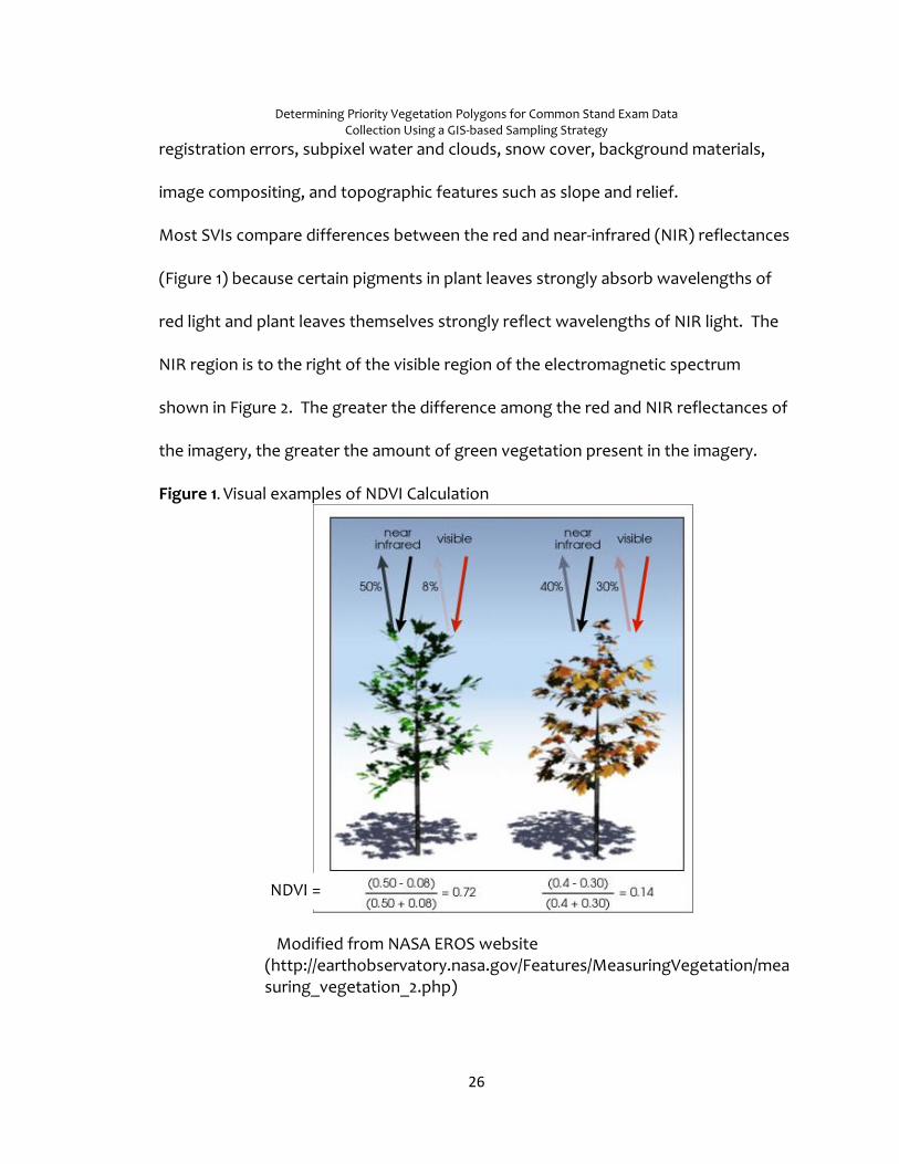
Most SVIs compare differences between the red and near-infrared (NIR) reflectances
(Figure 1) because certain pigments in plant leaves strongly absorb wavelengths of
red light and plant leaves themselves strongly reflect wavelengths of NIR light. The
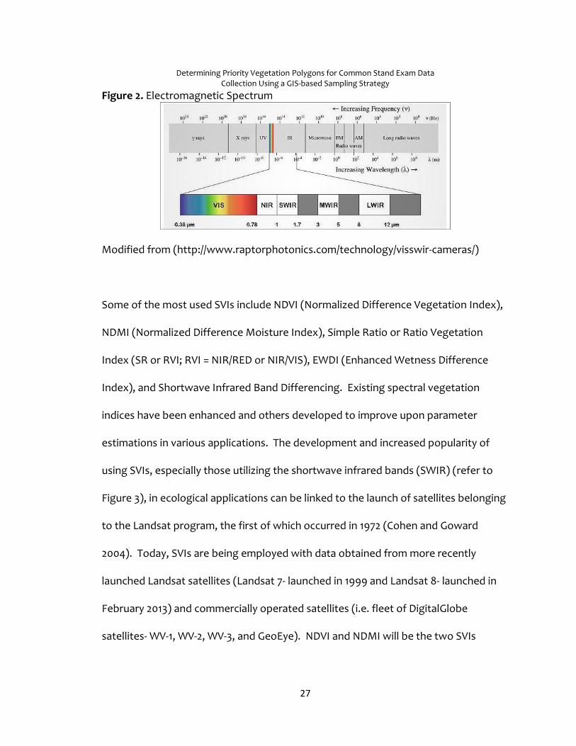
NIR region is to the right of the visible region of the electromagnetic spectrum
shown in Figure 2. The greater the difference among the red and NIR reflectances of
the imagery, the greater the amount of green vegetation present in the imagery.
Figure 1. Visual examples of NDVI Calculation
Modified from NASA EROS website (http://earthobservatory.nasa.gov/Features/MeasuringVegetation/measuring_vegetation_2.php)
NDVI =
Determining Priority Vegetation Polygons for Common Stand Exam Data Collection Using a GIS-based Sampling Strategy
27
Figure 2. Electromagnetic Spectrum
Modified from (http://www.raptorphotonics.com/technology/visswir-cameras/)
Some of the most used SVIs include NDVI (Normalized Difference Vegetation Index),
NDMI (Normalized Difference Moisture Index), Simple Ratio or Ratio Vegetation
Index (SR or RVI; RVI = NIR/RED or NIR/VIS), EWDI (Enhanced Wetness Difference
Index), and Shortwave Infrared Band Differencing. Existing spectral vegetation
indices have been enhanced and others developed to improve upon parameter
estimations in various applications. The development and increased popularity of
using SVIs, especially those utilizing the shortwave infrared bands (SWIR) (refer to
Figure 3), in ecological applications can be linked to the launch of satellites belonging
to the Landsat program, the first of which occurred in 1972 (Cohen and Goward
2004). Today, SVIs are being employed with data obtained from more recently
launched Landsat satellites (Landsat 7- launched in 1999 and Landsat 8- launched in
February 2013) and commercially operated satellites (i.e. fleet of DigitalGlobe
satellites- WV-1, WV-2, WV-3, and GeoEye). NDVI and NDMI will be the two SVIs

Determining Priority Vegetation Polygons for Common Stand Exam Data Collection Using a GIS-based Sampling Strategy
28
mentioned and discussed further in this paper as both NDVI and NDMI have been
frequently used to detect and monitor changes in forest stand condition in North
America. Additionally, NDVI was the index used to detect significantly changed
forested polygons on the GMUG over a 25 year period. Although I did not perform
the NDVI classifications, the NDVI classification conducted by RSAC was essential in
providing the changed polygon dataset that would serve as the initial input for the
GIS based sampling strategy created and employed in my Practicum project.
NDVI has been one of the most widely used SVIs in determining the relative density
and health of vegetation across the landscape. NDVI is calculated whereby the
difference between the near-infrared and red reflectances is divided by their sum.
NDVI = (NIR – RED)/(NIR +RED)
NDVI values range from -1 to 1. Areas of barren rock, sand, or snow usually show very
low NDVI values (0.1 or less), whereas sparse vegetation such as shrubs and
grasslands or senescing crops are typically associated with moderate NDVI values
(0.2 to 0.5). No green leaves also gives a value close to zero and dense vegetation is
associated with high NDVI values ranging from 0.6 to 1.0.
NDVI has been used in a variety of ecological applications to assess change detection
on local, regional, and global scales. For example, NDVI derived from MODIS data
was used to determine annual change detection rates from 2003 until 2005 for the
Albemarle-Pamlico Estuary System region in the southeastern US (Lunetta et al.
2006). In addition to determining change detection rates for the area, the study was

Determining Priority Vegetation Polygons for Common Stand Exam Data Collection Using a GIS-based Sampling Strategy
29
able to ascertain advantages and limitations of using MODIS NDVI data for
monitoring change detection at different local scales and within particular land
classification types. A second study derived NDVI from Landsat TM imagery to
examine vegetation cover density and productivity in Yosemite National Park,
California (Potter 2015). NDVI from 1986 to 2013 was analyzed and the findings
showed that overall NDVI decreased in Yosemite NP over the 20+ year time period
examined, contradicting previous predictions of increased NDVIs associated with
altered evapotranspiration fluxes and river flows for the Sierra Nevada. One last
example of how NDVI has been used is showing changes in vegetation cover density
in Hervi Watershed, Iran from 1976 to 2010 (Vahidi et al. 2013). Changes in NDVI
which signaled changes in vegetation cover density during the 34 year time period
were attributed to land use change such as increased urban area extent, road
building, mining activities, non-managed farming, and conversion of dense pastures
(Vahidi et al. 2013).
Similar to but still different from NDVI, NDMI is a measure of vegetation moisture, as
it is sensitive to changes in vegetation leaf structure and water content. It is
calculated as the difference between the NIR and the shortwave infrared (SWIR)
reflectances divided by their sum.
NDMI = (SWIR – NIR)/(SWIR + NIR)

Determining Priority Vegetation Polygons for Common Stand Exam Data Collection Using a GIS-based Sampling Strategy
30
It can be used to detect subtle changes in vegetation moisture conditions and can be
used for drought monitoring. There are several examples to illustrate its use over the
last decade. NDMI was used to assess areas of vegetation transition between the
years 1985 and 2010 on the central coast of California (Hsu et al. 2012). Another
application of NDMI was its use as an indication of flammability and spreadability of
fire while developing a fire risk model and creating a fire risk map displaying wildland
fire potential for the continental US (Zhang et al. 2014). NDMI has also been
employed in change detection applications for forest management such as detecting
stages of tree mortality from insect infestation (Goodwin et al 2008).
2.4.2 Change Detection of Tree Mortality The importance of SVIs in characterizing forest stands and the changes they undergo
when natural disturbances take place is well recognized (Skakun et al. 2003, Coops et
a. 2006, Wulder et al. 2006, Goodwin et al. 2008, Wulder et al. 2008, Meddens et al.
2011, Meigs et al. 2011). Much focus has been placed on large scale disturbances in
western North America such as bark beetle infestations and the resulting landscape-
scale tree mortality. Efforts have concentrated on determining the amount and type
of mortality that has occurred and predicting the direction and speed of mortality
into unaffected stands across the landscape. Several studies have investigated the
mortality caused by Mountain Pine Beetle (MPB) in Colorado, USA (Meddens et al.
2011, Meddens and Hicke 2014) and in the province of British Columbia, Canada
(Skakun et al. 2003, Coops et al. 2006, Wulder et al. 2006, Goodwin et al. 2008,

Determining Priority Vegetation Polygons for Common Stand Exam Data Collection Using a GIS-based Sampling Strategy
31
Wulder et al. 2008). Interest also has been placed in trying to understand spectral
trajectories of defoliator and bark beetle disturbances of varying duration and degree
across the landscape. Meigs et al. 2011 was able to detect both short and long
duration changes in spectral reflectance using LandTrendr, a Landsat time series
segmentation algorithm, indicating complex temporal dynamics in insect-affected
forests in the Cascade Range, Oregon, USA. All of these studies have added to the
knowledge about insect infestation from different agents and have led to a better
understanding in how insect infestations spread across the landscape and the nature
and duration of their existence.
2.5 Remote Sensing Application for Meeting Forest Management Objectives The development of forest management objectives is dependent upon the type of
planning being conducted (Wulder et al. 2005). More detail is necessary for
developing objectives that address land management direction over a local rather
than regional or global scales, especially if that direction is tactical or operational in
nature. On the other hand, coarse level data may be appropriate and adequate for
addressing strategic planning goals which can be broader in management direction.
For example, in the province of British Columbia, Canada, Landsat TM (Thematic
Mapper) and ETM+ (Enhanced Thematic Mapper) data, having a medium spatial
resolution of 30 meters, were used to map MPB red attack using multi-date scenes
(Skakun et al. 2003; Wulder et al. 2006, Goodwin et al. 2008). MPB attack has been
categorized in three different stages. Red attack is the stage of mortality before the

Determining Priority Vegetation Polygons for Common Stand Exam Data Collection Using a GIS-based Sampling Strategy
32
needles, which are red in color, drop to the ground. This stage occurs approximately
one year after bark beetles attack the tree. The first stage of attack is known as
green attack and as the stage suggests, the needles on the tree are still green at this
point in time. However, to guide field crews in determining exact locations of red
attack tree clusters and more precise detail in the extent and shape of red attack
stands across the landscape, high spatial resolution imagery from IKONOS (1 m for
panchromatic and 4 m for multispectral spatial resolution) and QuickBird (0.67 m for
panchromatic to 2.44 m for multispectral spatial resolution) were obtained and
classified (Coops et al. 2006; Wulder et al. 2008). In this case, the Landsat data filled
the purpose of bridging strategic and operational planning goals by mapping areas of
and identifying patterns of red attack across the studied landscape for strategic
planning whereas the IKONOS and QuickBird imagery acquisitions were utilized to
provide finer level detail for operational planning.
Strategic planning has played a vital role in developing and implementing Forest
Resource and Land Management Plans (FLMPs) for the Forests and Grasslands in the
USFS system. Strategic planning entails and relies on first understanding the existing
condition of the area of interest before determining a desired condition and what
management actions to apply to reach the desired state. Landsat imagery with 30
meter spatial resolution has played a major role in these types of investigations by
giving a synoptic view of spatial variation over the landscape. Landsat imagery has
Determining Priority Vegetation Polygons for Common Stand Exam Data Collection Using a GIS-based Sampling Strategy
33
been used in many ecological applications over the last 45 years to understand both
spatial and temporal pattern variations within ecosystems. The main reasons for its
prevalent utilization is that the detail the data offers meets the need of detecting
change at the landscape scale and there is over four decades of archived Landsat
imagery available for change detection analysis. Also, since 2008, archived Landsat
scenes are available to download from the United States Geological Survey (USGS)
EROS (Earth Resource Observation Satellites) website at no cost, making these data
economically feasible.
In applying Landsat imagery to forest management applications in the US, Meddens
and Hicke (2014) using Landsat TM 5 and Landsat ETM+ 7 imagery, were able to
estimate the MPB red stage tree mortality from 1996 to 2011 in the forested areas of
northcentral Colorado, USA. Mortality in the study area was found to move from
north to east earlier in the outbreak and then intensify in already attacked stands
later in the outbreak. Also, beetle outbreaks within 30 m grid cells were found to last
3 to 4 years, with grid cells in outbreak areas experiencing an average of 60%
mortality in total and 20% mortality per year. These results helped to increase the
understanding of bark beetle ecology and dynamics in the study area as well as
present methods that could be utilized to map and monitor other tree mortality
events. Unlike the studies that took place in Angstad Creek, BC, Canada (Wulder et
al. 2006; Wulder et al. 2008; Goodwin et al. 2008), this study occurred when mortality

Determining Priority Vegetation Polygons for Common Stand Exam Data Collection Using a GIS-based Sampling Strategy
34
was not expanding into new areas and it was deintensifying in areas that had already
been attacked. Salvage for many areas could have been a management strategy to
take during the second to third year of attack (red and gray attack stages) in riding
areas of dead lodgepole pine. However, because timber is typically not valuable
enough in the US to offset the cost of timber logging, harvest of these trees does not
happen over the scale needed to remove a majority of dead trees. Steep slopes and
inoperable terrain can make logging operations virtually impossible, with helicopter
logging along with its exorbitant cost being the only option to remove trees.
Instead, smaller areas that have been affected and can be accessed with traditional
logging equipment are salvaged. Additionally, the NEPA process can slow down the
process of implementing silvicultural prescriptions in general, even if those
prescriptions manage for recovery and resilience. Therefore, the findings of the
study did not direct management in operational tactics in dealing with the MPB
outbreak but did provide insight regarding how the infestation and resulting tree
mortality manifested across the landscape.
2.5.1 Use of High Spatial Resolution Satellite Data In many cases, high spatial resolution data can be utilized to address management
inquiries at both the strategic and tactical planning levels. Wulder et al. 2008 was
able to calculate the Red- Green Index (RGI), a ratio of the red to green wavelengths,
for forested stands in Angstad Creek, BC, Canada using QuickBird images acquired
annually during the growing seasons of 2003 to 2006. This measure was used in this

Determining Priority Vegetation Polygons for Common Stand Exam Data Collection Using a GIS-based Sampling Strategy
35
study because previously it had been shown to successfully detect red attack damage
of MPB (Coops et al. 2006). Once the change in RGI (∆RGI) was calculated for the
initial 2003 image in the time series, a ∆RGI threshold was determined and set for all
images, and field data was referenced to validate the imagery classifications. Red
attack damage was mapped for the study stands in each image with accuracy
percentages ranging from 89% to 93%. Additionally, the G:R (green to red attack)
ratio was calculated for each image/year. A G:R >1 indicates an increasing bark beetle
population whereas G:R < 1 indicates a decreasing population. The methods
identified the red attack stands in the study area as well as determined rates and
direction of the beetle attack. This information helped managers, foresters, and
researchers alike see the spatial variation of green and red attack across the study
area. Additionally, they were able to consider effective management strategies for
making stands more resilient to beetle attack and how this particular assessment
could be used in the future to help guide strategic planning of beetle management
(Wulder et al. 2008).
The GMUG is mainly focusing on forest stands affected by spruce beetle and other
related insects for treatment implementation. As previously mentioned, SBEADMR
treatments are planned to be implemented in the next ten years to help with
recovery and resiliency of Engelmann spruce. Although most of studies reviewed in
this chapter have examined the effects of bark beetle attack on lodgepole pine, a
Determining Priority Vegetation Polygons for Common Stand Exam Data Collection Using a GIS-based Sampling Strategy
36
similar approach to investigating bark beetle attack of Engelmann spruce could be
attempted. However, there may be challenges with utilizing similar methodologies
as Wulder et al. 2008 and Meddens and Hicke 2014. One major challenge is that
many times Engelmann spruce coexist with other conifer species within stands and
do not grow as pure stands as lodgepole pine often does. This can make it difficult to
use remotely sensed data and photo interpretation to differentiate between multiple
tree species growing within mixed conifer stands. This is especially true if both
species are being affected by infestations from different agents and both species
look similar to one another when viewed in imagery due to similar growth form. This
particular situation is taking place on the GMUG, specifically on the Uncompahgre
Plateau where subalpine fir is being killed by spruce budworm and Engelmann spruce
mostly by spruce beetle. Also, often times, the two species are difficult to distinguish
from one another in imagery. Many other photo interpretation characteristics and
clues other than color, texture, aspect, and slope are often used to make a decision
as to which species is being viewed. However, with any type of photo interpretation
there will be errors in interpretation. Keeping errors of commission and omission low
would be important to accomplish when applying methodologies from Wulder et al.
2008 or Meddens and Hicke, 2014 in using remotely sensed data to classify spruce
bark beetle infestation of GMUG spruce-fir forests.
Determining Priority Vegetation Polygons for Common Stand Exam Data Collection Using a GIS-based Sampling Strategy
37
Chapter Three
Methodology This study is comprised of four phases. Before I detail each of the four phases, I
provide descriptions of the FSVeg and FSVeg Spatial databases and their role in
vegetation polygon updates in general and not specifically for this Praticum. Also, I
explain the tools and applications used to perform GIS analyses and edits for this
Practicum.
3.2 Tools and other Applications I used ArcGIS 10.3.1, the Natural Resource Information System (NRIS) Geospatial
Interface (GI), and FS Veg Spatial to perform the GIS analyses for this study. I also
utilized ModelBuilder, an extension of ArcGIS, to automate and document repeatable
geoprocessing steps used to produce alternative outputs of priority polygons.
Priority indicates those polygons satisfying multiple criteria that in choosing them for
data collection would potentially lead to a lower cost for CSE data collection for the
mortality update project.
The GI allows the user to have access to “live” transactional data from NRIS that may
not be included in the attribute tables of the same spatial dataset residing on the
local Forest server or through the Spatial Database Engine (SDE) or published to the
Enterprise Data Warehouse (EDW). “Live” data refers to data that is the most
current up to date attribute data for that spatial dataset. The GI connects the NRIS
tabular data to the spatial data that can be obtained via the SDE and then the NRIS
Determining Priority Vegetation Polygons for Common Stand Exam Data Collection Using a GIS-based Sampling Strategy
38
data can be seen in the attribute table of the geospatial layer. I performed parts of
this project’s analysis with visualizations of NRIS and SDE data using the GI.
Specifically, the roads and activities layers used as input datasets in the models
created in this Practicum were retrieved from the GI.
3.3 Project Phases
3.1 Descriptions of FSVeg and FSVeg Spatial Field collected data characterizing forest stand conditions, which is also known as
CSE data, is used to update structure and composition of forested vegetation
polygons. The National Common Stand Exam data collection protocols found in the
FSVeg (Field Sampled Vegetation) Common Stand Exam User Guide are used for
determining the number and arrangement of plots in each polygon from which to
collect CSE data, the specific measurements taken in each plot, and the plot size for
each measurement taken (USDA Forest Service, 2015). The CSE data collected in the
field is uploaded to and stored in the FSVeg tabular database.
Like FSVeg, FSVeg Spatial is a Forest Service database application that holds tabular
data that characterizes forested vegetation polygons. However, unlike FSVeg, FSVeg
Spatial is a national geodatabase system that consists of vegetation polygons and
CSE spatial point locations and associated relationship data tables that display
information on lifeform, layer, species, size, canopy or crown cover percentages, and
local cover types for each unique vegetation polygon delineation. FSVeg is a
database that is not GIS based and is solely dedicated to storing field collected CSE
Determining Priority Vegetation Polygons for Common Stand Exam Data Collection Using a GIS-based Sampling Strategy
39
data, until the data can be used for project analysis and creating reports detailing
timber stand metrics. This database also provides the plot level data to update
tabular records for vegetation polygon attributes in FSVeg Spatial.
Each region of the US Forest Service follows the FSVeg Spatial User Guide to create,
maintain, and update spatial delineations and attributes of vegetation polygons, but
each can have a separate protocol to address specific regional needs relating to
vegetation polygon maintenance. Region 2 follows a particular protocol outlined in
the R2 Supplement of the FSVeg Spatial User Guide (2016b). More specifically,
Region 2 utilizes a R2 FS Veg Spatial Polygon Vegetation Attributes Form (Figure 3) to
collect information for each polygon such as sampling recorder, species survey
method, sample date, purpose code (method used to collect data, i.e. photo
interpretation, stand exam, walkthrough, quick plot stand exam, etc.), horizontal
continuity, crown condition, canopy closure or canopy cover, tree species, tree and
shrub size class, and dead percentage of each vegetation cover layer. This form may
be completed during photo interpretation of the polygon(s) or during walkthrough
visits. If CSE data is to be collected for polygons, a forester visits those polygons in
the field or views aerial imagery in GIS to determine if polygons need to be spatially
redelineated in FSVeg Spatial prior to designing plot layout. If he/she deems that
polygons need to be redelineated, the R2 attributes form is completed for each
polygon during the field visit/walkthrough and prior to CSE data collection to ensure
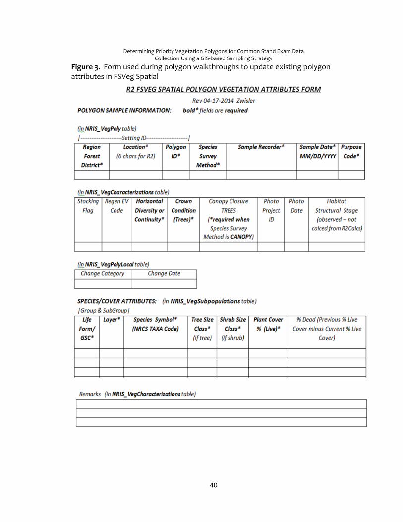
Determining Priority Vegetation Polygons for Common Stand Exam Data Collection Using a GIS-based Sampling Strategy
40
Figure 3. Form used during polygon walkthroughs to update existing polygon attributes in FSVeg Spatial

Determining Priority Vegetation Polygons for Common Stand Exam Data Collection Using a GIS-based Sampling Strategy
41
the necessary edits both to spatial and tabular data are made and posted in FSVeg
Spatial.
The R2 attributes form and a map showing topographic relief or imagery with the re-
delineations of the polygons drawn on it are provided to the FSVeg Spatial editor if
edits are not performed by the data collector himself/herself, in order for the editor
to accurately redraw boundaries of the polygons needing redelineations and make
changes to polygon attributes in FSVeg Spatial. Then, the newly edited polygon
boundaries are used to layout plots for CSE data collection. Recently an ArcGIS tool
was developed that allows an editor to update live and dead percentages for all
vegetation layers in FSVeg Spatial using CSE plot data rather than data collected
during a walkthrough visit. If the decision is made to use this tool, spatial
redelineation still takes place prior to plot layout and CSE data collection, if needed.
Hence, some vegetation may be missed when collecting plot data as compare to data
collected during a walkthrough.
3.3.1 Phase I Figure 5 shows the general order in which methods occurred to address the
objectives of this project. The reader can view a more detailed version of Figure 4 in
Appendix B (Figure B-1). The detail provided in Figure B-1 provides the reader
understanding of all of the specific steps taken in each phase to address the research
questions and ultimately produce the final priority polygons for CSE data collection.
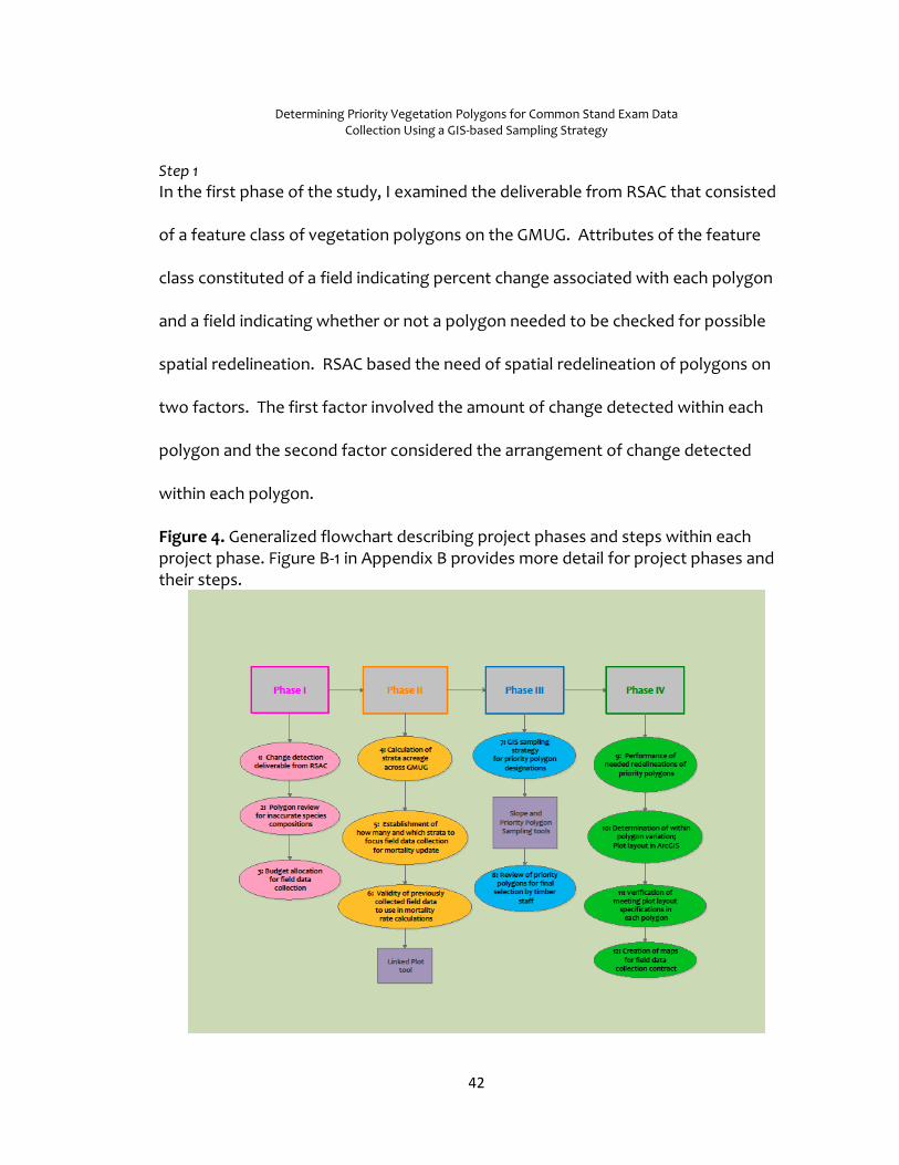
Determining Priority Vegetation Polygons for Common Stand Exam Data Collection Using a GIS-based Sampling Strategy
42
Step 1
In the first phase of the study, I examined the deliverable from RSAC that consisted
of a feature class of vegetation polygons on the GMUG. Attributes of the feature
class constituted of a field indicating percent change associated with each polygon
and a field indicating whether or not a polygon needed to be checked for possible
spatial redelineation. RSAC based the need of spatial redelineation of polygons on
two factors. The first factor involved the amount of change detected within each
polygon and the second factor considered the arrangement of change detected
within each polygon.
Figure 4. Generalized flowchart describing project phases and steps within each project phase. Figure B-1 in Appendix B provides more detail for project phases and their steps.

Determining Priority Vegetation Polygons for Common Stand Exam Data Collection Using a GIS-based Sampling Strategy
43
RSAC completed a change detection analysis that identified vegetation polygons in
which 0.001% to 100% of the individual cells or pixels exhibited vegetation change.
This change was derived by analyzing Landsat imagery from 1989 and comparing it to
the same type of imagery from 2014. The two temporal sets of imagery were used to
compute a differenced NDVI for each scene. This calculation resulted in a continuous
difference layer with positive and negative values used to quantify the change in
vegetation that had occurred over the 25 year period within each of the polygons
examined. GMUG selected a threshold of 15% to focus updates on those forested
vegetation polygons displaying 15% or more change in NDVI. These polygons are
referred to as changed polygons from this point forward in the Practicum document.
RSAC looked at landscape pattern metrics of the changed pixels by calculating
fragmentation statistics for each polygon to determine those polygons in which the
change occurred within a contiguous area or if change was distributed throughout
the polygon. Five acres or more of contiguous change adjacent to at least five acres
of no change within a polygon indicated to RSAC that the polygon needed to be
checked for redelineation using aerial imagery. If it was verified from the aerial
imagery that redelineation was needed, polygon modifications occurred prior to CSE
data collection, if selected as a priority polygon, and prior to attribute update.
Step 2
As a part of Phase I, I interacted with the silviculturists and foresters from Ouray,
Norwood, and Gunnison Ranger Districts to gather their knowledge regarding areas

Determining Priority Vegetation Polygons for Common Stand Exam Data Collection Using a GIS-based Sampling Strategy
44
within each of their districts that may have inaccurate species compositions recorded
in FSVeg Spatial. I have initiated but not completed this step, a topic that will be
addressed in Chapter 5.
Step 3
I visited with GMUG GIS and timber staff to ascertain the amount of money allocated
to CSE data collection for the mortality update project. This figure changed multiple
times during the Practicum project. For this reason, I incorporated flexibility within
the project to accommodate and adjust for shifts in funding. If the amount of funds
changed during the project, the number and location of priority polygons to include
in the contract bid could be easily modified to reflect this change. Unfortunately, a
decrease in funds available for field data collection was more likely to occur than an
increase.
3.3.2 Phase II
Cluster Analysis
A cluster analysis on the vegetation polygons was performed to determine the
number and type of strata that exist across the GMUG. The process was not a
component of this Practicum project; instead, RSAC performed this analysis prior to
the initiation of this Practicum. The purpose of the cluster analysis was to ensure
that sampled polygons represented all of the different tree species and canopy cover
percentage combinations found across the GMUG to adequately capture the
variation in mortality rates that exist across the GMUG. The details regarding the
Determining Priority Vegetation Polygons for Common Stand Exam Data Collection Using a GIS-based Sampling Strategy
45
cluster analysis can be found in Stam (2015a) and Stam (2016). The completion of the
cluster analysis was essential in moving forward in this Practicum and finishing Phase
II.
GMUG planning, timber, and GIS staff decided the strata to be included in the CSE
data collection and the tree mortality update. This decision was based on several
factors. Budget played a large role in this decision as well as the extent of mortality
found within a stratum. Another factor was the number of polygons within a stratum
that already had relatively current CSE data associated with them to adequately
describe existing vegetative conditions within those polygons and for the strata with
which the polygons were grouped. In general, a greater amount of valid and useful
field data already collected in polygons of a stratum and available to use in the
mortality rate calculations meant less time and money spent on field data collection
in that particular stratum for the mortality update project. Steps 4 and 5
The expectation was that more mortality would be seen in the strata that contained
mostly Engelmann spruce and subalpine fir, as forest health aerial survey data
collected annually showed the majority of tree damage and “fading” occurring in
Picea engelmanni and Abies spp. on the GMUG for the last several years (USDA Forest
Service, 2016a). Additionally, a large amount of attention has been focused on the
increase in SAD observed on the GMUG over the last ten to fifteen years. Although

Determining Priority Vegetation Polygons for Common Stand Exam Data Collection Using a GIS-based Sampling Strategy
46
aspen is not a highly sought after timber product on the GMUG, it is important for
species diversity and valued by many people for its beauty. Aspen stands on the
GMUG bring in noted tourism dollars to surrounding communities during the summer
and fall months. Therefore, planning, timber, and GIS staff agreed upon the strata
consisting of Engelmann spruce, subalpine fir, aspen, and combinations thereof as
priority from which to select polygons to include in the tree mortality update. To
help with solidifying the decision on which strata to focus the mortality update, I
calculated the polygon acreage associated with each stratum in ArcGIS using the
RSAC deliverable feature class in step 4 of Phase II. Step 5 consisted of analyzing and
comparing the approximate cost of field data collection for different acreage
percentages of the priority strata. GMUG’s original goal was to collect field data
from a 10% sample of the total acreage associated with a stratum for each priority
strata.
Step 6 In step 6 of Phase II, I identified CSE plot data that had previously been collected on
the Forests on or after 2010 that was still valid for building tree mortality rule sets. I
created a tool using ArcGIS ModelBuilder to perform this step. Although this tool
was implemented in Phase II, I have explained the tool in Chapter Three, Phase IV, in
the same section where the other tool descriptions are located, as I thought it was
appropriate to keep all tool descriptions together to help the reader better
understand why and how the tools were constructed and implemented.
Determining Priority Vegetation Polygons for Common Stand Exam Data Collection Using a GIS-based Sampling Strategy
47
The time that had elapsed since data collection within a polygon affected the validity
of CSE data for describing existing vegetative conditions and hence affected whether
or not the data would be used in building tree mortality rule sets. This decision was
based on a discussion that tool place with the SO timber staff, Matt Bienkowski. CSE
data that was collected prior to 2010 was automatically considered too old for
describing existing vegetative conditions and not used in building mortality rule sets.
Also, I referenced low NDVI year data and CSE plot locations in ArcGIS to determine if
the data suggested that tree mortality had taken place prior to or after CSE data
collection within the polygons. I have given a more detailed explanation of the low
NDVI year data in Phase III used in this analysis. Similarly, I loaded activity polygon
data from the EDW using the GI and viewed it with CSE point location data to verify
no vegetation altering activities (VAAs) had occurred within polygons since CSE data
collection.
The EDW is the Forest Service one stop shop for accessing FS and non-FS spatial data.
Its purpose is to integrate data from various sources, in formats that can be shared
across the Forest Service and even with the public. Data cannot be edited in the EDW
but the EDW publishes and refreshes USFS spatial datasets that have been edited by
each Forest and Grassland in their respective Forest/Grassland SDE instance on a
frequent and continual basis. The Activity Polygons dataset is refreshed in the EDW
every 24 hours and displays areas in which VAAs have occurred.
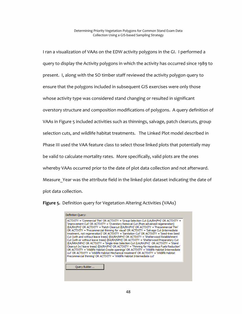
Determining Priority Vegetation Polygons for Common Stand Exam Data Collection Using a GIS-based Sampling Strategy
48
I ran a visualization of VAAs on the EDW activity polygons in the GI. I performed a
query to display the Activity polygons in which the activity has occurred since 1989 to
present. I, along with the SO timber staff reviewed the activity polygon query to
ensure that the polygons included in subsequent GIS exercises were only those
whose activity type was considered stand changing or resulted in significant
overstory structure and composition modifications of polygons. A query definition of
VAAs in Figure 5 included activities such as thinnings, salvage, patch clearcuts, group
selection cuts, and wildlife habitat treatments. The Linked Plot model described in
Phase III used the VAA feature class to select those linked plots that potentially may
be valid to calculate mortality rates. More specifically, valid plots are the ones
whereby VAAs occurred prior to the date of plot data collection and not afterward.
Measure_Year was the attribute field in the linked plot dataset indicating the date of
plot data collection.
Figure 5. Definition query for Vegetation Altering Activities (VAAs)

Determining Priority Vegetation Polygons for Common Stand Exam Data Collection Using a GIS-based Sampling Strategy
49
During the winter of 2017, I will archive the invalid points in FSVeg Spatial and give the
valid points along with reports entailing sample design for CSE data collection to the
SO timber staff for review. SO timber staff will make the final determination on the
validity of plot data and which datasets will be used in building tree mortality rule
sets.
Based on an estimate for CSE data collection for the San Juan National Forest and an
IDIQ (indefinite delivery/indefinite quantity) contract plot cost for the Rio Grande
National Forest, costs of CSE data collection on these two Forests ranged anywhere
between $63 to $78 per plot ( Sally Zwisler, personal communication, October 20,
2015). IDIQ contracts for CSE stand exam data collection have run approximately $80
to $90 for the Ouray RD of the GMUG since 2014. These contracts haven been
established for data collection on the Uncompahgre Plateau of the Ouray RD from
2014 to 2018. TEAMS (Talent, Expertise, Agility, Mobility, and Simplicity) Enterprise
Unit’s costs for CSE data collection on the GMUG were found to be consistently more
expensive, costing approximately $200 per plot (Carol Howe, personal
communication, September 30, 2016). To reduce cost, SO timber staff strived to
secure an IDIQ contract for CSE data collection tasks.
For this Practicum, I used an estimate of $100 per plot to yield a cost estimate for CSE
data collection. Using this estimate, a budget of $35,000 would yield 350 plots.
Major factors that affected cost per plot were the plot location in relation to the
distance from roads in relatively good condition indicated by an operational

Determining Priority Vegetation Polygons for Common Stand Exam Data Collection Using a GIS-based Sampling Strategy
50
maintenance level of 3, 4, or 5 and manageable terrain (<40% slope) for hiking to and
within the polygon. I incorporated these factors and other related factors in Phase IV
when I created the GIS sampling strategy. I also considered travel time to the
polygons from the GMUG SO office and RD offices; however, I did not include this
criterion into polygon sampling, because after further discussion with the GIS and SO
timber staff, they did not feel a least cost path analysis was necessary or worth the
time to conduct to try to further reduce the cost of contract CSE data collection. A
least cost path analysis would have resulted in route lengths from a GMUG
administrative site to each polygon of interest, thereby providing more information
regarding travel distance and time to reach each priority polygon. Regardless of
whether or not a least cost path analysis was performed, the purpose of the
sampling strategy was to maximize the amount of plots to be visited in the field and
minimize the amount of funds needed for and spent on CSE data collection for the
mortality update project. Nevertheless, the least cost path analysis would have
pinpointed those priority polygons from which crews would be most efficient in
collecting CSE data. Greater efficiency meant lower cost for contract data collection.
3.3.3 Phase III
Tool Creation I created six tools using Modelbuilder in ArcMap whose main purpose, when
collectively implemented, was to narrow down polygons from which to collect field
data, keeping in mind factors and traits of polygons that could increase data

Determining Priority Vegetation Polygons for Common Stand Exam Data Collection Using a GIS-based Sampling Strategy
51
collection costs. The six tools created were 1) linked plot tool, 2) slope tool, 3) first
priority polygon sampling tool, 4) second priority polygon sampling tool, 5) third
priority polygon sampling tool, and 6) final priority polygon sampling tool. I
constructed two tools, the linked plot and slope tools, that each generated a feature
class to be used in other tools. Both feature classes served as inputs into the first
priority polygon sampling tool which then calculated fields for linked plot and slope
status for each polygon. These field calculations were then used in subsequent
polygon selections by the second and third priority polygon sampling tools. I
constructed the linked plot tool in Phase II. However, I have provided its explanation
in this section with the descriptions of the other five tools to help the reader better
understand the role of each tool and how and when each tool was created during the
Practicum.
Each of the three polygon sampling tools produced a feature class output that
identified first, second, and third priority polygons, respectively. I designed the tools
to start with an input feature class that consisted only of changed polygons; the
reason is that they would be the best polygons to collect field data from to capture
the amount of mortality that has occurred on the GMUG to date. I devised the final
priority polygon sampling tool to first merge first, second, and third priority polygon
selections into one feature class and then to perform an intersection of VAAs
discussed in Phase II (Figure 5) with the priority polygon feature class. Those
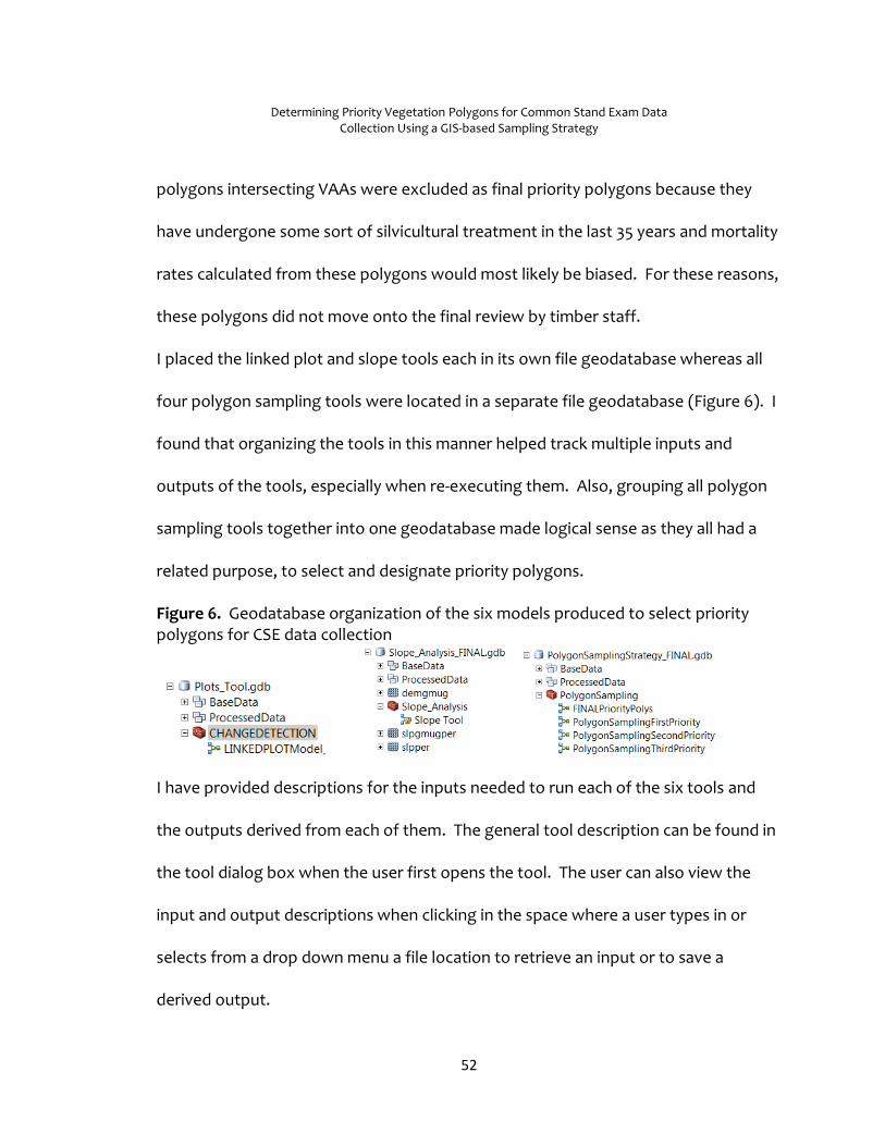
Determining Priority Vegetation Polygons for Common Stand Exam Data Collection Using a GIS-based Sampling Strategy
52
polygons intersecting VAAs were excluded as final priority polygons because they
have undergone some sort of silvicultural treatment in the last 35 years and mortality
rates calculated from these polygons would most likely be biased. For these reasons,
these polygons did not move onto the final review by timber staff.
I placed the linked plot and slope tools each in its own file geodatabase whereas all
four polygon sampling tools were located in a separate file geodatabase (Figure 6). I
found that organizing the tools in this manner helped track multiple inputs and
outputs of the tools, especially when re-executing them. Also, grouping all polygon
sampling tools together into one geodatabase made logical sense as they all had a
related purpose, to select and designate priority polygons.
Figure 6. Geodatabase organization of the six models produced to select priority polygons for CSE data collection
I have provided descriptions for the inputs needed to run each of the six tools and
the outputs derived from each of them. The general tool description can be found in
the tool dialog box when the user first opens the tool. The user can also view the
input and output descriptions when clicking in the space where a user types in or
selects from a drop down menu a file location to retrieve an input or to save a
derived output.
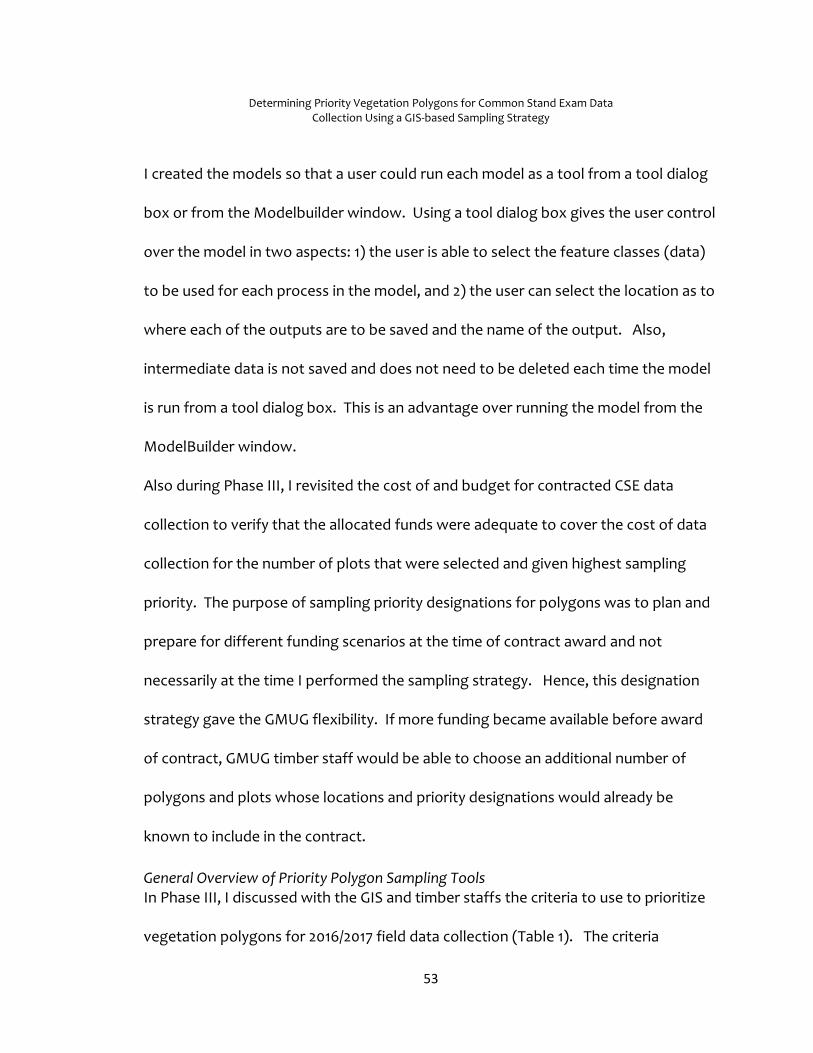
Determining Priority Vegetation Polygons for Common Stand Exam Data Collection Using a GIS-based Sampling Strategy
53
I created the models so that a user could run each model as a tool from a tool dialog
box or from the Modelbuilder window. Using a tool dialog box gives the user control
over the model in two aspects: 1) the user is able to select the feature classes (data)
to be used for each process in the model, and 2) the user can select the location as to
where each of the outputs are to be saved and the name of the output. Also,
intermediate data is not saved and does not need to be deleted each time the model
is run from a tool dialog box. This is an advantage over running the model from the
ModelBuilder window.
Also during Phase III, I revisited the cost of and budget for contracted CSE data
collection to verify that the allocated funds were adequate to cover the cost of data
collection for the number of plots that were selected and given highest sampling
priority. The purpose of sampling priority designations for polygons was to plan and
prepare for different funding scenarios at the time of contract award and not
necessarily at the time I performed the sampling strategy. Hence, this designation
strategy gave the GMUG flexibility. If more funding became available before award
of contract, GMUG timber staff would be able to choose an additional number of
polygons and plots whose locations and priority designations would already be
known to include in the contract.
General Overview of Priority Polygon Sampling Tools In Phase III, I discussed with the GIS and timber staffs the criteria to use to prioritize
vegetation polygons for 2016/2017 field data collection (Table 1). The criteria

Determining Priority Vegetation Polygons for Common Stand Exam Data Collection Using a GIS-based Sampling Strategy
54
included factors such as within-polygon terrain, polygon acreage, type of land
ownership within each polygon, and polygon’s distance from decently maintained
roads. Also, we valued polygons characterized as having potential suitable timber
and not associated with valid, recently collected field data as priority candidates. We
finalized the criteria to incorporate into the GIS sampling strategy and chose the
criteria that would be used in each sampling tool. I modified two criteria for the
second priority sampling tool that were used in the first priority sampling tool. They
were the criteria concerned with polygon distance from a maintained road and
polygon location in relation to Wilderness, CRAs, and other specially designated
areas. I excluded two criteria used in the second priority sampling tool from the third
priority sampling tool. Moreover, I used one new criterion in the third priority
Table 1. Criteria used in each of the three priority polygon sampling tools to select polygons for CSE data collection
Tool Polygon Criteria Used for Priority Selection
First Priority Polygon Sampling
1) Significantly changed polygons within priority ctrata
2) Slopes < 40% or only 5% of area having slopes >= 40%
3) Not having valid CSE data
3) Size >= 30 and < 300 acres
4) Not having any NONFS lands within AND do not intersect NONFS lands
5) Not within Wilderness, CRAs, or other specially designated areas
6) Within 1/2 mile of roads with OML of 3, 4, or 5
7) Within potentially suitable timber areas
Second Priority Polygon Sampling
1) Significantly changed polygons within priority strata
2) Slopes < 40% or only 5% of area having slopes >= 40%
3) Not having valid CSE data
3) Size >= 30 and < 300 acres
4) No NONFS jurisdiction within or do not intersect NONFS lands
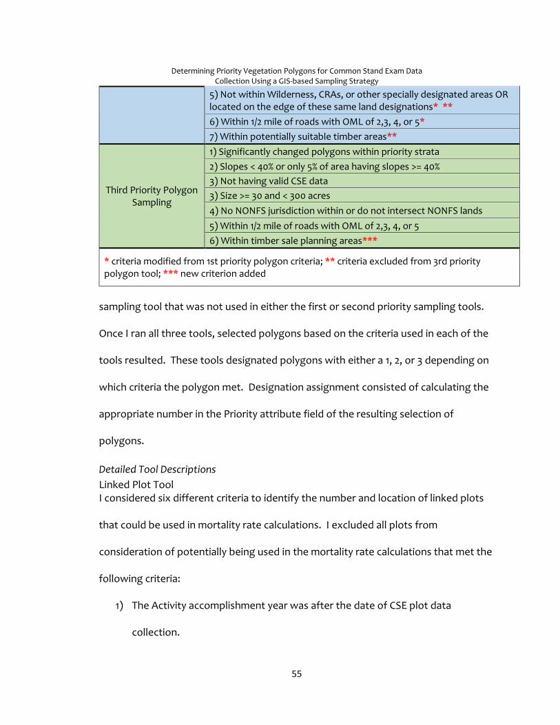
Determining Priority Vegetation Polygons for Common Stand Exam Data Collection Using a GIS-based Sampling Strategy
55
5) Not within Wilderness, CRAs, or other specially designated areas OR located on the edge of these same land designations* **
6) Within 1/2 mile of roads with OML of 2,3, 4, or 5*
7) Within potentially suitable timber areas**
Third Priority Polygon Sampling
1) Significantly changed polygons within priority strata
2) Slopes < 40% or only 5% of area having slopes >= 40%
3) Not having valid CSE data
3) Size >= 30 and < 300 acres
4) No NONFS jurisdiction within or do not intersect NONFS lands
5) Within 1/2 mile of roads with OML of 2,3, 4, or 5
6) Within timber sale planning areas***
* criteria modified from 1st priority polygon criteria; ** criteria excluded from 3rd priority polygon tool; *** new criterion added
sampling tool that was not used in either the first or second priority sampling tools.
Once I ran all three tools, selected polygons based on the criteria used in each of the
tools resulted. These tools designated polygons with either a 1, 2, or 3 depending on
which criteria the polygon met. Designation assignment consisted of calculating the
appropriate number in the Priority attribute field of the resulting selection of
polygons.
Detailed Tool Descriptions
Linked Plot Tool I considered six different criteria to identify the number and location of linked plots
that could be used in mortality rate calculations. I excluded all plots from
consideration of potentially being used in the mortality rate calculations that met the
following criteria:
1) The Activity accomplishment year was after the date of CSE plot data
collection.

Determining Priority Vegetation Polygons for Common Stand Exam Data Collection Using a GIS-based Sampling Strategy
56
I used timber harvest and hazardous fuel treatment activity polygon
layers (VAAs) to determine the date of when the vegetation in those
polygons had been altered by treatment activities in relation to the
date of when the CSE data had been collected.
2) The year of the low point NDVI was greater than the year that plot data had
been collected.
I converted the lowest NDVI year raster to a polygon feature class
before it was used in the analysis.
Each pixel of the raster represented the year(s) in which NDVI
(greenness) was the lowest. It was broken up into 2 year categories
(1994-1995, 1996-1997, 1998-1999,…, 2014-2015). For instance, if a pixel
had a value of 2002, then that meant that NDVI was the lowest in 2002
or 2003. This would mean that if there was a field sample on this pixel
with a sample date after 2003, then the field data should be able to be
used in mortality rate calculations.
This was not a change detection raster. Every pixel had a year value
because all pixels had an NDVI low point. For example, a pixel might
have had a value of 2006, but this only meant that the lowest NDVI
value was observed during that time. This could have been caused by a
dry year or it could have represented an actual disturbance. The main

Determining Priority Vegetation Polygons for Common Stand Exam Data Collection Using a GIS-based Sampling Strategy
57
point being that as long as plot data were collected after the NDVI low
point year, then any change that happened at that plot should already
have been completed.
3) The measure year attribute of the plot feature class was less than 2010, which
indicated that data had been collected prior to 2010.
4) The plots were measured in a polygon in which the strata was not one of the
chosen priority strata.
5) The remaining plots did not span across the polygon when viewing plots and
polygons simultaneously with 1 ft 2012 resource imagery or 1 m 2011 or 2015
NAIP imagery. This situation implied that the plot data did not adequately
quantify stand conditions of the polygon in which the data was collected.
6) The sample design of the plots resulting from the GIS analysis met the CSE
data guidelines and specifications outlined in Zwisler (2016b). This step still
remains to be performed by the GMUG timber staff.
I incorporated the first four criteria into the linked plot tool (Figures 7 and 8). I
examined plots after tool execution to see if they met the fifth criterion. Polygons
meeting the sixth criterion will be determined the winter/spring of 2017.
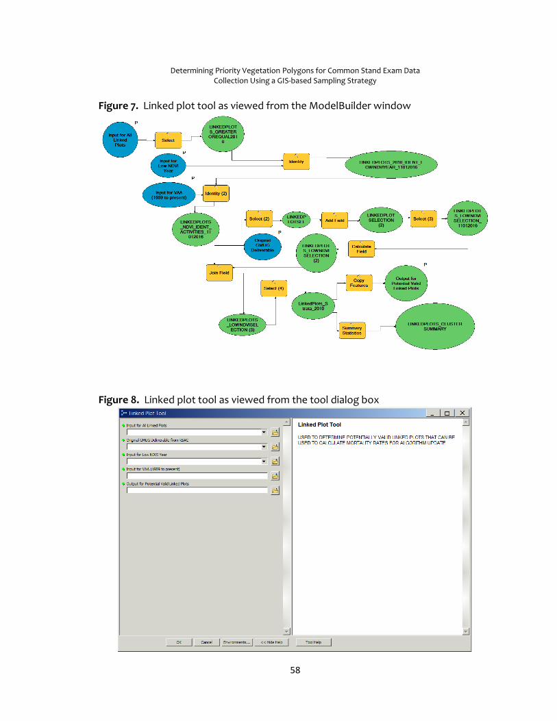
Determining Priority Vegetation Polygons for Common Stand Exam Data Collection Using a GIS-based Sampling Strategy
58
Figure 7. Linked plot tool as viewed from the ModelBuilder window
Figure 8. Linked plot tool as viewed from the tool dialog box

Determining Priority Vegetation Polygons for Common Stand Exam Data Collection Using a GIS-based Sampling Strategy
59
Slope Tool The slope tool (Figures 9 and 10) created an output feature class that was then used
in the priority polygon sampling tools. The basis of the output was to categorize
those areas within all of the changed polygons into two categories: 1) slopes less
than or equal to 40 percent, and 2) slopes greater than 40 percent. The final output
of the slope tool was a field in the attribute table of the changed polygons that
indicated which polygons had slopes less than or equal to 40 percent or 5% or less of
their area having slopes less than or equal to 40 percent. I, along with the timber
staff, agreed that these polygons would be less difficult to hike and maneuver
around in and would be the easiest from which to collect data in regards to terrain
steepness.

Determining Priority Vegetation Polygons for Common Stand Exam Data Collection Using a GIS-based Sampling Strategy
60
Figure 9. Slope tool viewed from the ModelBuilder window

Determining Priority Vegetation Polygons for Common Stand Exam Data Collection Using a GIS-based Sampling Strategy
61
Figure 10. Slope tool viewed from the tool dialog box.
First Priority Polygon Sampling Criteria First priority polygons were those that would be the first of the changed polygons to
review for plot layout and CSE data collection. These polygons met the slope
criterion, having slopes less than or equal to 40% or 5% or less of the acreage having
slopes greater than or equal to 40%. Crews were also able to access these polygons
within at least a half mile from decently maintained roads as indicated by the
incorporation of criterion six into the first tool (Table 1). I defined decent
maintenance as those roads having an operational maintenance level (OML) of a 3, 4,
or 5. Furthermore, first and second priority tools targeted polygons with potentially
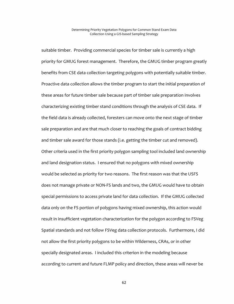
Determining Priority Vegetation Polygons for Common Stand Exam Data Collection Using a GIS-based Sampling Strategy
62
suitable timber. Providing commercial species for timber sale is currently a high
priority for GMUG forest management. Therefore, the GMUG timber program greatly
benefits from CSE data collection targeting polygons with potentially suitable timber.
Proactive data collection allows the timber program to start the initial preparation of
these areas for future timber sale because part of timber sale preparation involves
characterizing existing timber stand conditions through the analysis of CSE data. If
the field data is already collected, foresters can move onto the next stage of timber
sale preparation and are that much closer to reaching the goals of contract bidding
and timber sale award for those stands (i.e. getting the timber cut and removed).
Other criteria used in the first priority polygon sampling tool included land ownership
and land designation status. I ensured that no polygons with mixed ownership
would be selected as priority for two reasons. The first reason was that the USFS
does not manage private or NON-FS lands and two, the GMUG would have to obtain
special permissions to access private land for data collection. If the GMUG collected
data only on the FS portion of polygons having mixed ownership, this action would
result in insufficient vegetation characterization for the polygon according to FSVeg
Spatial standards and not follow FSVeg data collection protocols. Furthermore, I did
not allow the first priority polygons to be within Wilderness, CRAs, or in other
specially designated areas. I included this criterion in the modeling because
according to current and future FLMP policy and direction, these areas will never be

Determining Priority Vegetation Polygons for Common Stand Exam Data Collection Using a GIS-based Sampling Strategy
63
intentionally treated with thinning, harvest, or prescribed burning activities. GMUG
management preferred to target polygons for data collection that can and are
planned to be treated in the next five years to reach treatment accomplishment
goals. Additionally, higher costs for field data collection on Wilderness, CRAs, or
other specially designated areas could have ensued because crews would have
needed more travel time to access most of these areas compared to other FS lands.
This is because most specially designated lands on the GMUG, such as Wilderness
areas, are accessed by driving on unmaintained roads and then hiking the rest of the
way. Although some non-specially designated lands of the GMUG may be a distance
from FS offices, many of these areas can be reached by driving on roads receiving
some sort of annual road maintenance, thereby resulting in less time to arrive at
these areas as compared to many of GMUG’s specially designated areas.
The last two criterion included in the priority polygon sampling tools were choosing
polygons already associated with valid field data and those within a size range of 30
to 300 acres (Table 1). Polygons characterized by having valid CSE data would help
reduce the amount and cost of field data collection because instead of collecting new
data in those polygons, the already collected data could be used in mortality rate
calculations. I have given a description of what constitutes validity of field data in
Phase II, Step 6 of Chapter 3. SO timber and GIS staff deliberated and chose the
range of polygon size with the purpose of maximizing the amount of data collected

Determining Priority Vegetation Polygons for Common Stand Exam Data Collection Using a GIS-based Sampling Strategy
64
compared to the amount of time needed for data collection to take place within each
polygon. This decision was also influenced by the advice and suggestion of Sally
Zwisler, retired R2 Vegetation Applications Coordinator. Keeping polygon sizes
smaller than 300 but greater than 30 acres minimized the amount of area traversed
and time spent by a crew when collecting data while increasing the probability of
capturing realistic snapshots of tree mortality found within each polygon.
Once I executed the tool (Figures 11 and 12), the fields shown in Table 2 were
calculated. I designed the tool to place a ‘Y’ in the appropriate field of the attribute
table when that polygon met the criteria represented by that field, except for
Wild_Other_CRAs2 in which case a ‘Y-E’ was calculated.
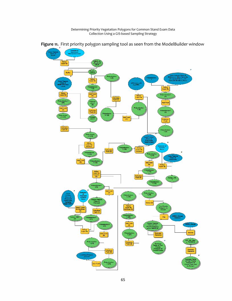
Determining Priority Vegetation Polygons for Common Stand Exam Data Collection Using a GIS-based Sampling Strategy
65
Figure 11. First priority polygon sampling tool as seen from the ModelBuilder window
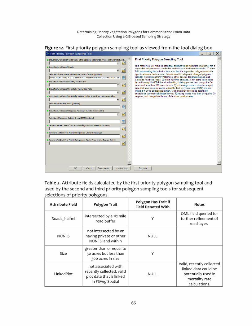
Determining Priority Vegetation Polygons for Common Stand Exam Data Collection Using a GIS-based Sampling Strategy
66
Figure 12. First priority polygon sampling tool as viewed from the tool dialog box
Table 2. Attribute fields calculated by the first priority polygon sampling tool and used by the second and third priority polygon sampling tools for subsequent selections of priority polygons.
Attrribute Field Polygon Trait Polygon Has Trait if Field Denoted With
Notes
Roads_halfmi intersected by a 1/2 mile
road buffer Y
OML field queried for further refinement of
road layer.
NONFS not intersected by or
having private or other NONFS land within
NULL
Size greater than or equal to
30 acres but less than 300 acres in size
Y
LinkedPlot
not associated with recently collected, valid plot data that is linked
in FSVeg Spatial
NULL
Valid, recently collected linked data could be potentially used in
mortality rate calculations.
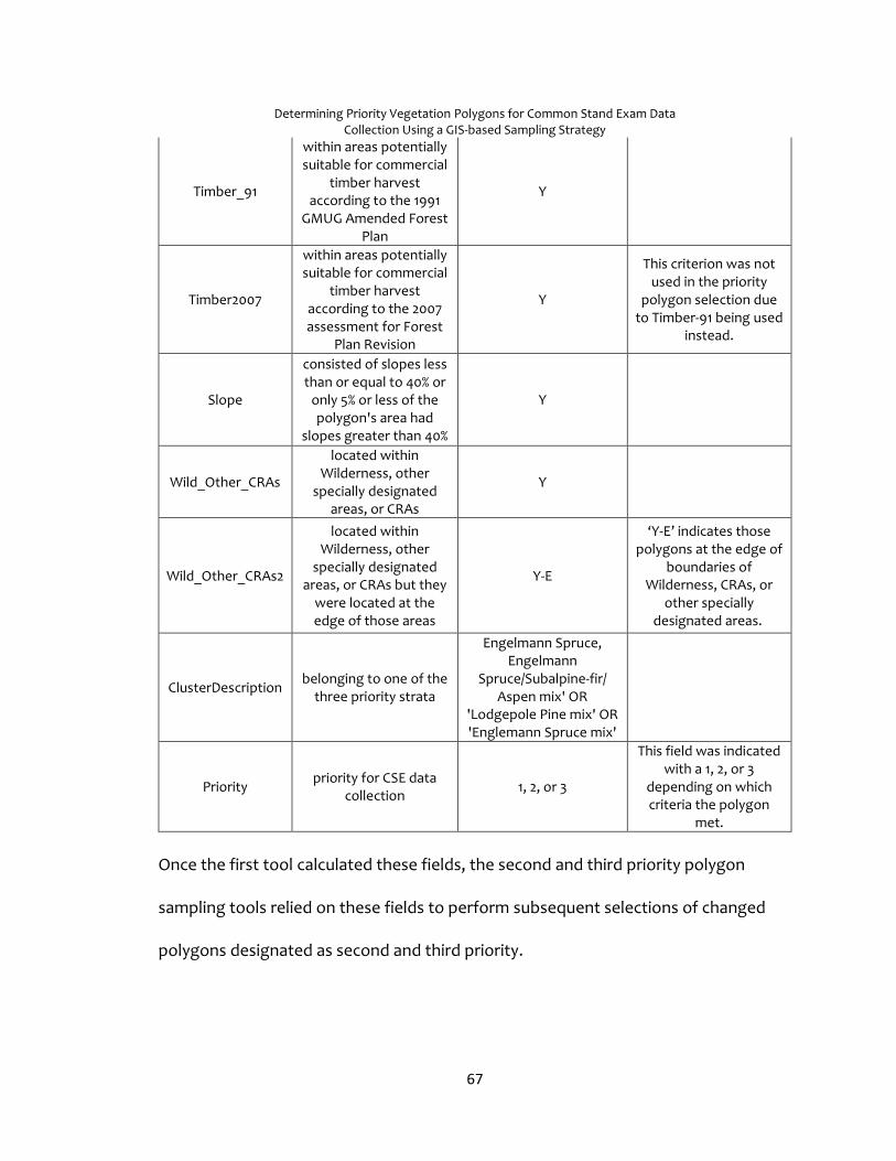
Determining Priority Vegetation Polygons for Common Stand Exam Data Collection Using a GIS-based Sampling Strategy
67
Timber_91
within areas potentially suitable for commercial
timber harvest according to the 1991
GMUG Amended Forest Plan
Y
Timber2007
within areas potentially suitable for commercial
timber harvest according to the 2007 assessment for Forest
Plan Revision
Y
This criterion was not used in the priority
polygon selection due to Timber-91 being used
instead.
Slope
consisted of slopes less than or equal to 40% or
only 5% or less of the polygon's area had
slopes greater than 40%
Y
Wild_Other_CRAs
located within Wilderness, other
specially designated areas, or CRAs
Y
Wild_Other_CRAs2
located within Wilderness, other
specially designated areas, or CRAs but they
were located at the edge of those areas
Y-E
‘Y-E’ indicates those polygons at the edge of
boundaries of Wilderness, CRAs, or
other specially designated areas.
ClusterDescription belonging to one of the
three priority strata
Engelmann Spruce, Engelmann
Spruce/Subalpine-fir/ Aspen mix' OR
'Lodgepole Pine mix' OR 'Englemann Spruce mix'
Priority priority for CSE data
collection 1, 2, or 3
This field was indicated with a 1, 2, or 3
depending on which criteria the polygon
met.
Once the first tool calculated these fields, the second and third priority polygon
sampling tools relied on these fields to perform subsequent selections of changed
polygons designated as second and third priority.

Determining Priority Vegetation Polygons for Common Stand Exam Data Collection Using a GIS-based Sampling Strategy
68
Overlaying First Priority Polygons with Vegetation Altering Activities I intersected first priority polygons with VAAs that had occurred on the GMUG since
1989 (refer to Figure 5) to complete the last step in determining the total number of
first priority polygons left for CSE data collection and determine whether criteria
needed to be excluded from or modified during continued future sampling in order
to increase the number of polygons for data collection.
I excluded polygons that had experienced VAAs because mortality rates calculated
from CSE data collected from these polygons would not reflect accurate amounts of
mortality from insect and disease infestations. The reason is that VAAs usually result
in the removal of any dead trees, except for leaving some snags in the stands for
wildlife. Therefore, activities listed in Figure 6 would most likely result in dead
overstory vegetation being felled and removed from the polygons, thereby affecting
or decreasing mortality found within the treated stands and biasing mortality rate
calculations that would be used in the update algorithm.
Due to many first priority polygons being excluded for field sampling as a result of
VAA intersection, I supplemented the priority polygon sampling strategy with two
additional tools, the second and third priority polygon sampling tools. These tools
selected and assigned polygons as second or third priority meeting the criteria for
such designations (Table 1). I created these two tools to ultimately increase the
acreage, through polygon selection, in each of the three priority strata from which

Determining Priority Vegetation Polygons for Common Stand Exam Data Collection Using a GIS-based Sampling Strategy
69
CSE data would be collected and to move more closely toward reaching the objective
of collecting field data from 10% of the total acreage for each of three priority strata.
Second Priority Polygon Sampling Criteria Second priority polygons were those that would be the second to review for plot
layout. First, I removed first priority polygons from the changed polygon layer,
including the ones intersected by VAAs, and saved the remaining changed polygons
to a separate feature class labeled Polyselection2. This layer was the sample of
changed polygons used in the second tool from which second priority polygons
would be selected.
I used all of the same criteria in the second priority polygon sampling tool as in the
first priority polygon sampling tool except I modified the selection to also include
those polygons located at the edge of boundaries of Wilderness, CRAs, and other
specially designated areas and those within a half mile of roads having OML of 2, 3, 4,
or 5. Inclusion of these criteria loosened up the restrictions of priority polygons not
being allowed to exist within specially designated areas or accessed by roads with an
OML of 2. OML 2 roads can be accessed only by high-clearance vehicles having four
wheel drive capability and are not suitable for passenger cars. OML 3 roads are
maintained to provide adequate drainage to reduce potholing and washboarding
although user comfort and convenience is a low priority when maintaining the
surface of these type of roads. OML 4 and 5 roads are maintained to provide for a
high to moderate degree of user comfort and provide for convenience and the

Determining Priority Vegetation Polygons for Common Stand Exam Data Collection Using a GIS-based Sampling Strategy
70
protection of investment and resource values. Surfaces of OML 4 and 5 roads are
either paved asphalt, chip sealed, or gravel surface. Broadening criteria five and six
from the first tool in the second priority polygon sampling tool allowed for more
polygons to be considered for CSE data collection (Table 1). The tool (Figure 13)
designated these polygons as second priority for data collection as these polygons
would most likely take a longer time to access due to OML 2 roads not being
maintained and travel to most specially designated areas, in which some second
priority polygons are located, require crews to drive on OML 2 roads. The tool used
Structured Query Language (SQL) to perform a final selection of second priority
polygons. I created SQL expressions of the fields listed in Table 3 to highlight those
polygons to be designated as second priority.

Determining Priority Vegetation Polygons for Common Stand Exam Data Collection Using a GIS-based Sampling Strategy
71
Figure 13. Second priority polygon sampling tool as viewed from the ModelBuilder window

Determining Priority Vegetation Polygons for Common Stand Exam Data Collection Using a GIS-based Sampling Strategy
72
Table 3. Attribute fields and SQL expressions used by second priority polygon sampling tool to select and designate second priority polygons
Attribute Field SQL Expression Additional Expression
Used
Roads_halfmi Rds_halfmi = ‘Y’ Operational
Maintenance of Roads <>1
NONFS NONFS IS NULL
Size Size = 'Y'
LinkedPlot LINKEDPLOT IS NULL
Timber_91 Timber_91 = 'Y'
Slope Slope = 'Y'
Wild_Other_CRAs and
Wild_Other_CRAs2
Wild_Other_CRAs IS NULL OR Wild_Other_CRAs2 = ‘Y-E’
ClusterDescription
ClusterDescription = 'Engelmann
spruce/Subalpine-fir/Aspen' OR ClusterDescription = 'Lodgepole Pin mix' OR
ClusterDescription = 'Englemann Spruce mix'
Third Priority Polygon Sampling Criteria Third priority polygon sampling tool used all of the same criteria as the first and
second tools. However, it did not restrict the selection to those polygons within
specially designated areas or within areas having potentially suitable timber as it did
in the first and second tools. The main focus of the third tool was to select any
polygons within the north and west zone timber sale planning areas not already
previously selected from the first and second tools. I did not include east zone

Determining Priority Vegetation Polygons for Common Stand Exam Data Collection Using a GIS-based Sampling Strategy
73
timber sale planning area (Gunnison RD) in the third tool because the feature class
detailing this area was not provided to me at the time. As a way to prevent the
exclusion of any east zone polygons planned for upcoming timber sale, I relied on the
Gunnison RD silviculturist to notice any polygons within the east zone timber sale
planning areas not selected by any of the sampling tools during his review of the
polygons and performance of plot layout. My expectation was that as a result of his
review, he would add to the final priority polygon feature class any within the east
zone timber sale planning area that had not been previously selected. Also, I did not
include linked plot criterion into the third tool because I decided to review the
polygon selections for any valid and recent plot data after the third tool had been
executed.
Figure 14. Third priority polygon sampling tool as viewed from the ModelBuilder window
The tool (Figure 14) designated polygons selected by SQL expressions listed in Table
4 as third priority polygons.

Determining Priority Vegetation Polygons for Common Stand Exam Data Collection Using a GIS-based Sampling Strategy
74
Table 4. Attributes fields and SQL expressions used by the third priority polygon sampling tool to select and designate third priority polygons
Attribute Field SQL Expression Additional Expression
Used
Roads_halfmi Rds_halfmi = ‘Y’ Operational
Maintenance of Roads <>1
NONFS NONFS IS NULL
Size Size = 'Y'
Slope Slope = 'Y'
ClusterDescription
ClusterDescription = 'Engelmann
spruce/Subalpine-fir/Aspen' OR
ClusterDescription = 'Lodgepole Pin mix' OR
ClusterDescription = 'Englemann Spruce mix'
Final Priority Polygon Tool and VAA Intersection with Priority Polygons Using the final priority polygon tool, first, second, and third priority polygons were
merged into one feature class (Figure 14). The tool then intersected the merged
feature class with the VAA feature class obtained from the GI (Figure 5). I then
reviewed the VAA intersection with the polygons to determine which polygons had
at least a quarter of their area affected by VAA instead of only a boundary touching a
treatment. The polygons who had a quarter or more of their area affected by VAA
were not included in the final priority polygon feature class. I then delivered this
polygon feature class to the SO timber staff for final review.

Determining Priority Vegetation Polygons for Common Stand Exam Data Collection Using a GIS-based Sampling Strategy
75
Figure 15. Final priority polygon tool as viewed from the ModelBuilder window
Review of Final Priority Polygons The SO timber staff reviewed the final priority polygons to ensure agreement of
those polygons selected by the GIS sampling strategy for CSE data collection. Final
priority polygons located on only the Gunnison Ranger District were given to the
Gunnison RD silviculturist for review. Both the SO timber staff and GIS staff agreed
that this additional review for Gunnison polygons was needed due to a majority of
change due to tree mortality having taken place on the Gunnison RD in comparison
to other districts on the GMUG and a majority of priority polygons selected for 2016
and 2017 CSE data collection being situated on the Gunnison RD. Additionally, the
Gunnison RD silviculturist’s help was needed and valued as he has over 30 years’

Determining Priority Vegetation Polygons for Common Stand Exam Data Collection Using a GIS-based Sampling Strategy
76
experience working on the Gunnison. He knows the general condition of and best
access to most forested polygons on the district. For this project, he gave valued
feedback on the results of the GIS sampling strategy and remote sensing analysis
that reinforced the premise to combine data analysis results with field knowledge
during decision making process. In addition to reviewing the accessibility to
polygons for data collection, he marked those changed polygons he knew needed to
be spatially redelineated, regardless of which polygons were flagged by RSAC for
redelineation. He also helped with redelineation of these polygons prior to plot
layout.
3.3.4 Phase IV
Polygon Redelineation The Gunnison RD sivilculturist and I redelineated polygons using 1 meter multiband
aerial imagery from the National Agriculture Imagery Program (NAIP) acquired in 2011
and 2015 and 30 cm multiband resource imagery acquired in 2012. The USFS obtained
resource imagery for the GMUG during June through September of 2012. 2011 and
2015 NAIP imagery acquisitions ranged from July to September of 2011 and 2015,
respectively.
All delineations were performed in ArcMap. However, I performed delineations using
the FSVeg Spatial application and the silviculturist redelineated polygons using the
ArcMap editor toolbar. He used this method to save time in completing
redelineations and to be able to finish plot layout in time for the 2016 contract
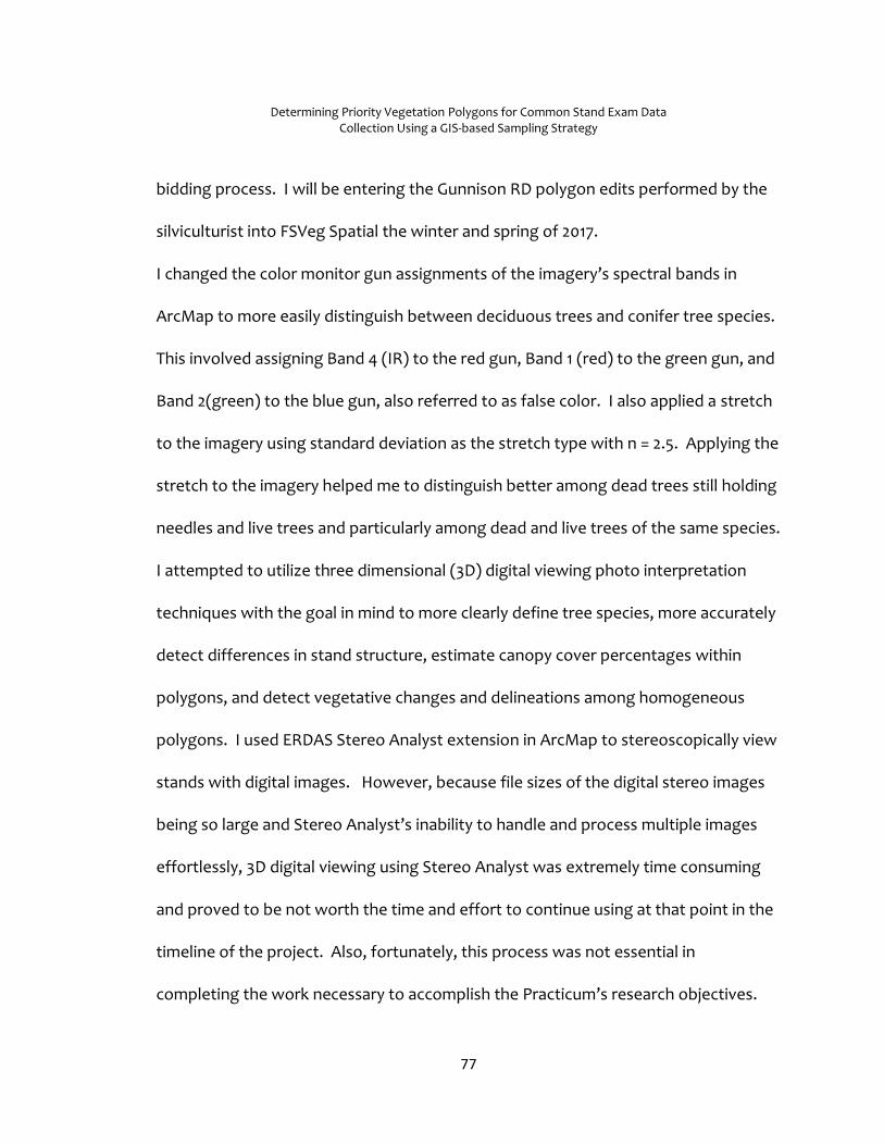
Determining Priority Vegetation Polygons for Common Stand Exam Data Collection Using a GIS-based Sampling Strategy
77
bidding process. I will be entering the Gunnison RD polygon edits performed by the
silviculturist into FSVeg Spatial the winter and spring of 2017.
I changed the color monitor gun assignments of the imagery’s spectral bands in
ArcMap to more easily distinguish between deciduous trees and conifer tree species.
This involved assigning Band 4 (IR) to the red gun, Band 1 (red) to the green gun, and
Band 2(green) to the blue gun, also referred to as false color. I also applied a stretch
to the imagery using standard deviation as the stretch type with n = 2.5. Applying the
stretch to the imagery helped me to distinguish better among dead trees still holding
needles and live trees and particularly among dead and live trees of the same species.
I attempted to utilize three dimensional (3D) digital viewing photo interpretation
techniques with the goal in mind to more clearly define tree species, more accurately
detect differences in stand structure, estimate canopy cover percentages within
polygons, and detect vegetative changes and delineations among homogeneous
polygons. I used ERDAS Stereo Analyst extension in ArcMap to stereoscopically view
stands with digital images. However, because file sizes of the digital stereo images
being so large and Stereo Analyst’s inability to handle and process multiple images
effortlessly, 3D digital viewing using Stereo Analyst was extremely time consuming
and proved to be not worth the time and effort to continue using at that point in the
timeline of the project. Also, fortunately, this process was not essential in
completing the work necessary to accomplish the Practicum’s research objectives.

Determining Priority Vegetation Polygons for Common Stand Exam Data Collection Using a GIS-based Sampling Strategy
78
I created a training guide for remote sensing interpretation in the spring of 2016 in an
effort to train the interpreter’s eye on the various vegetation types on the GMUG. I
examined and compared recently collected field data of selected polygons to the
species composition and structure identified through the imagery interpretation of
the same polygons. The ultimate purpose of the guide was to help a photo
interpreter know what different tree species looked like in imagery to maximize the
accuracy of tree species identification.
Plot Layout Step 10 (Figure 4) involved considering the variation within each polygon to address
the primary objective of the stand exam data collection. The primary objective was
to determine the number of plots from which data needed to be collected to
accurately describe the dead tree percentage found within that polygon. A second
objective was to adequately describe stand composition and structure for each
polygon. The purpose of meeting the second objective was to provide stand exam
data for polygons lacking any past and recent data collection and that were
delineated by and attributes assigned from photo interpretation alone. I referenced
FSVeg CSE User Guide protocol standards to complete this part of step 10.
The FSVeg CSE User Guide describes within polygon variation by calculating the
coefficient of variation (CV). CV is the standard deviation expressed as percent of a
variable’s mean. The variable chosen is based on its relevancy in addressing the
objective of the analysis. For example, if the question of the analysis was to
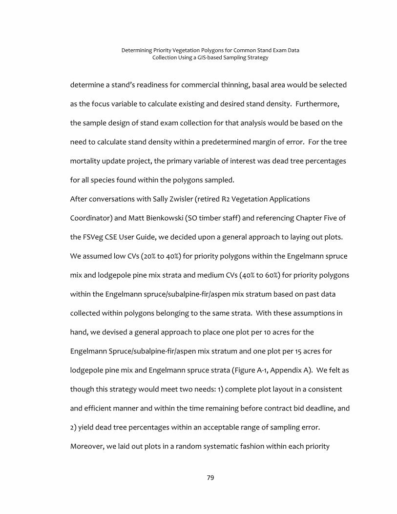
Determining Priority Vegetation Polygons for Common Stand Exam Data Collection Using a GIS-based Sampling Strategy
79
determine a stand’s readiness for commercial thinning, basal area would be selected
as the focus variable to calculate existing and desired stand density. Furthermore,
the sample design of stand exam collection for that analysis would be based on the
need to calculate stand density within a predetermined margin of error. For the tree
mortality update project, the primary variable of interest was dead tree percentages
for all species found within the polygons sampled.
After conversations with Sally Zwisler (retired R2 Vegetation Applications
Coordinator) and Matt Bienkowski (SO timber staff) and referencing Chapter Five of
the FSVeg CSE User Guide, we decided upon a general approach to laying out plots.
We assumed low CVs (20% to 40%) for priority polygons within the Engelmann spruce
mix and lodgepole pine mix strata and medium CVs (40% to 60%) for priority polygons
within the Engelmann spruce/subalpine-fir/aspen mix stratum based on past data
collected within polygons belonging to the same strata. With these assumptions in
hand, we devised a general approach to place one plot per 10 acres for the
Engelmann Spruce/subalpine-fir/aspen mix stratum and one plot per 15 acres for
lodgepole pine mix and Engelmann spruce strata (Figure A-1, Appendix A). We felt as
though this strategy would meet two needs: 1) complete plot layout in a consistent
and efficient manner and within the time remaining before contract bid deadline, and
2) yield dead tree percentages within an acceptable range of sampling error.
Moreover, we laid out plots in a random systematic fashion within each priority
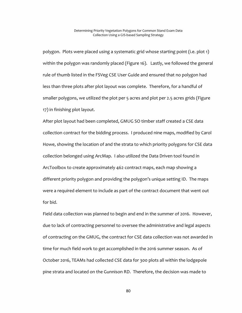
Determining Priority Vegetation Polygons for Common Stand Exam Data Collection Using a GIS-based Sampling Strategy
80
polygon. Plots were placed using a systematic grid whose starting point (i.e. plot 1)
within the polygon was randomly placed (Figure 16). Lastly, we followed the general
rule of thumb listed in the FSVeg CSE User Guide and ensured that no polygon had
less than three plots after plot layout was complete. Therefore, for a handful of
smaller polygons, we utilized the plot per 5 acres and plot per 2.5 acres grids (Figure
17) in finishing plot layout.
After plot layout had been completed, GMUG SO timber staff created a CSE data
collection contract for the bidding process. I produced nine maps, modified by Carol
Howe, showing the location of and the strata to which priority polygons for CSE data
collection belonged using ArcMap. I also utilized the Data Driven tool found in
ArcToolbox to create approximately 462 contract maps, each map showing a
different priority polygon and providing the polygon’s unique setting ID. The maps
were a required element to include as part of the contract document that went out
for bid.
Field data collection was planned to begin and end in the summer of 2016. However,
due to lack of contracting personnel to oversee the administrative and legal aspects
of contracting on the GMUG, the contract for CSE data collection was not awarded in
time for much field work to get accomplished in the 2016 summer season. As of
October 2016, TEAMs had collected CSE data for 300 plots all within the lodgepole
pine strata and located on the Gunnison RD. Therefore, the decision was made to

Determining Priority Vegetation Polygons for Common Stand Exam Data Collection Using a GIS-based Sampling Strategy
81
extend the field data collection period into 2017, finishing up data collection by
October 2017. The contract for 2017 CSE data collection will be created during the
winter of 2017, for bidding to begin spring of the same year.
Figure 16. Systematic grids used for plot layout in Step 10 of Phase IV.
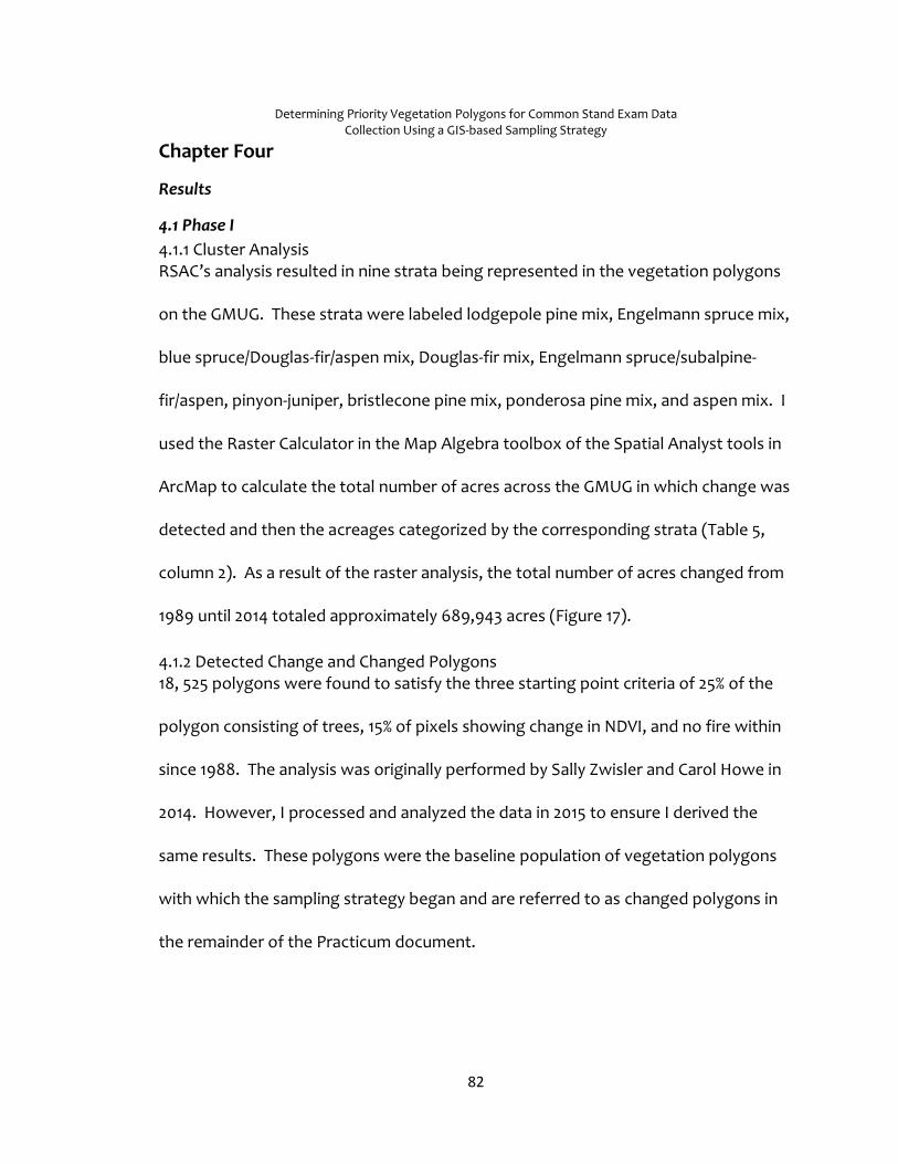
Determining Priority Vegetation Polygons for Common Stand Exam Data Collection Using a GIS-based Sampling Strategy
82
Chapter Four
Results
4.1 Phase I
4.1.1 Cluster Analysis RSAC’s analysis resulted in nine strata being represented in the vegetation polygons
on the GMUG. These strata were labeled lodgepole pine mix, Engelmann spruce mix,
blue spruce/Douglas-fir/aspen mix, Douglas-fir mix, Engelmann spruce/subalpine-
fir/aspen, pinyon-juniper, bristlecone pine mix, ponderosa pine mix, and aspen mix. I
used the Raster Calculator in the Map Algebra toolbox of the Spatial Analyst tools in
ArcMap to calculate the total number of acres across the GMUG in which change was
detected and then the acreages categorized by the corresponding strata (Table 5,
column 2). As a result of the raster analysis, the total number of acres changed from
1989 until 2014 totaled approximately 689,943 acres (Figure 17).
4.1.2 Detected Change and Changed Polygons 18, 525 polygons were found to satisfy the three starting point criteria of 25% of the
polygon consisting of trees, 15% of pixels showing change in NDVI, and no fire within
since 1988. The analysis was originally performed by Sally Zwisler and Carol Howe in
2014. However, I processed and analyzed the data in 2015 to ensure I derived the
same results. These polygons were the baseline population of vegetation polygons
with which the sampling strategy began and are referred to as changed polygons in
the remainder of the Practicum document.

Determining Priority Vegetation Polygons for Common Stand Exam Data Collection Using a GIS-based Sampling Strategy
83
Table 5. Number of acres by strata showing detected change ranging from 1% to 100% from 1989 until 2014 within the GMUG boundary.
Cluster Description
All Changed
Acres
Ranking Based on
# of Changed
Acres
Acreage of polygons in which 15% of
pixels changed **
Total Acreage of 15% Changed
Polygons**
Percentage of acreage within 15% changed
polygons that is actually changed
No Change 2,464,664
Engelmann Spruce/Subalpine
fir/Aspen mix* 292,760 1 275,189 433,326 64
Lodgepole Pine Mix*
133,436 2 125,978 230,043 55
Engelmann Spruce Mix*
120,026 3 105,696 156,293 68
Aspen Mix 47,929 4 34,005 92,618 37
Pinyon Juniper 37,084 5 26,201 76,624 34
Douglas-fir Mix 21,171 6 17,366 40,157 43
Ponderosa Pine Mix
17,804 7 7,802 18,932 41
Blue Spruce/Douglas-
fir/Aspen mix 4,698 8 4,342 8,462 51
Bristlecone Pine Mix
3,205 9 2,579 5,161 50
Null Cluster Description
11,830
Total Acres Changed=
689,943 599,158 1,061,615 56
*Priority stratum, ** Polygons with no fire since 1988, 25% treed, within forest boundary

Determining Priority Vegetation Polygons for Common Stand Exam Data Collection Using a GIS-based Sampling Strategy
84
Figure 17. All change (>0% to 100%) in NDVI from 1989 until 2014 on the GMUG. NDVI change is in blue.
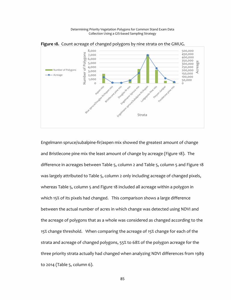
Determining Priority Vegetation Polygons for Common Stand Exam Data Collection Using a GIS-based Sampling Strategy
85
Figure 18. Count acreage of changed polygons by nine strata on the GMUG.
Engelmann spruce/subalpine-fir/aspen mix showed the greatest amount of change
and Bristlecone pine mix the least amount of change by acreage (Figure 18). The
difference in acreages between Table 5, column 2 and Table 5, column 5 and Figure 18
was largely attributed to Table 5, column 2 only including acreage of changed pixels,
whereas Table 5, column 5 and Figure 18 included all acreage within a polygon in
which 15% of its pixels had changed. This comparison shows a large difference
between the actual number of acres in which change was detected using NDVI and
the acreage of polygons that as a whole was considered as changed according to the
15% change threshold. When comparing the acreage of 15% change for each of the
strata and acreage of changed polygons, 55% to 68% of the polygon acreage for the
three priority strata actually had changed when analyzing NDVI differences from 1989
to 2014 (Table 5, column 6).
050,000100,000150,000200,000250,000300,000350,000400,000450,000500,000
01,0002,0003,0004,0005,0006,0007,0008,000
Acr
eag
e
Nu
mb
er
of
Po
lyg
on
s
Strata
Number of Polygons
Acreage
Determining Priority Vegetation Polygons for Common Stand Exam Data Collection Using a GIS-based Sampling Strategy
86
4.2 Phase II
4.2.1 Priority Strata Due to a limited budget, GIS and timber staff decided to reduce the number of strata
to include in the polygon sampling strategy from nine to three. The three strata
selected were the strata in which the most change had been detected. In those
three strata, change was detected in 13,894 polygons across 819,663 acres. These
polygons belonged to Engelmann spruce mix, Engelmann spruce/subalpine-fir/aspen,
and lodgepole pine mix (Figure 18 and Table 6). CSE data collection needs to occur
on approximately 43,000 acres for Engelmann spruce/subalpine-fir/aspen stratum,
23,000 acres for lodgepole pine stratum, and 16,000 acres for Engelmann spruce
stratum to achieve the objective of collecting data from 10% of the acreage for each
priority strata. The approximate cost of CSE data collection from these 82,000 acres,
depending on the sampling intensity used, would be $691,000. For all analyses
performed for this Practicum other than for the results displayed in Table 5, acreages
of changed polygons such as the ones reported in Figure 18 and Table 6 were used.
4.2.2 Linked Plot Tool Results I performed linked plot analysis so that we could be better informed as to whether
any existing data could be potentially used in the mortality rate calculations for the
three priority strata. I found a total of 1030 linked plots to be potentially valid to use
in mortality rate calculations for six strata, three of which were priority strata. After
selecting only those plots located in polygons belonging to priority strata, 304 plots
remained for consideration. Data had been collected anywhere from 2010 to 2015 in

Determining Priority Vegetation Polygons for Common Stand Exam Data Collection Using a GIS-based Sampling Strategy
87
Table 6. Approximate cost of field data collection using a 10% sample for each of the 3 priority strata.
Cluster Description
Number of
Changed Polygons*
Acres of Changed Polygons
10% of Total
Acreage
Cost of 1 plot per
10 acres**
Cost of 1 plot per 15
acres**
Engelmann Spruce/Subalpine-
fir/Aspen 7,106 433,326 43,333 $433,326
Lodgepole Pine mix 3,297 230,043 23,004 $153,362
Engelmann Spruce mix 3,491 156,293 15,629 $104,195
Aspen mix 2,321 92,618 9,262
Pinyon-Juniper 579 76,624 7,662
Douglas-fir mix 933 40,157 4,016
Ponderosa pine mix 372 18,932 1,893
Blue spruce/Douglas-fir/Aspen mix
206 8,462 846
Bristlecone pine mix 220 5,161 516
Total= 18,525 1,061,615 106,161 $690, 883
* Changed polygons are those whereby at least 15% of pixels are changed, had not experienced fire since 1988, and at least 25% treed.
**An approximate cost of $100 per plot was used for these cost calculations. This cost was based on costs generated in previous contracts on the GMUG as well as two other National Forests in Region 2.
Determining Priority Vegetation Polygons for Common Stand Exam Data Collection Using a GIS-based Sampling Strategy
88
56 polygons belonging to the three priority strata (Figure 19). More specifically, data
had been collected in forty five plots over 218 acres for the Engelmann spruce mix,
122 plots over 652 acres for the lodgepole pine mix, and 137 plots over 2,878 acres for
the Engelmann spruce/ subalpine-fir/aspen mix (Figure 19). Polygons associated with
the Engelmann spruce/ subalpine-fir/aspen stratum had been flagged for
redelineation by RSAC. Flagged for redelineation meant that the polygon needed to
be viewed against the backdrop of aerial imagery at a scale of 1:24000 or larger to
verify that the polygon was no longer homogeneous. In this case, the linked plots
associated with polygons needing redelineation would not be used in calculating
mortality rates. Four polygons had been flagged by RSAC as possibly needing
redelineation. Plot data had been collected from 51 plots within these four polygons.
If after review, the polygons do no portray homogeneous stand conditions, the
decision will be made not to use the polygon’s CSE data in building tree mortality rule
sets and plots for those polygons will be archived in FSVeg Spatial. I performed an
initial review of polygon boundaries against the backdrop of NAIP 2015 aerial imagery
and as a result, all polygon delineations used to collect linked plot data did not
appear to need redelineation. Final review of this data by SO timber staff will take
place in the winter of 2017; after the final review, timber staff will make the final
determination as to whether the plot data will be used for calculating mortality rates
for the change detection project. Moreover, sample design criteria of the selected

Determining Priority Vegetation Polygons for Common Stand Exam Data Collection Using a GIS-based Sampling Strategy
89
linked plots will be included in the review to ensure the design used meets the
requirements for the change detection project outlined in Zwisler, 2016. To perform
this task, I will run a sample design report for the desired setting IDs of the polygons
in the FSVeg tabular application to be used in the review.
Figure 19. Bar graph indicating number of possibly valid linked plots to use in building mortality rule sets.
4.3 Phase III
4.3.1 Slope Tool The slope analysis revealed that 2,277,223 acres had slopes less than or equal to 40
percent and 877,242 acres consisted of slopes greater than 40 percent across the
GMUG. When I converted the slope raster into a polygon feature class and
intersected with vegetation polygons, I found that 6,675 changed polygons had
slopes less than or equal to 40 percent or no more than 5% of their area to be greater
than 40 percent. These 6,675 polygons equated to 297,700 acres. I then
incorporated the final output of the slope analysis in the first polygon sampling tool
to add the slope field to the attribute table of the changed polygon feature class.
20
6
19
57
27
2
122
7
44
0
20
40
60
80
100
120
140
2010 2014 2015 2010 2014 2015 2014
Engelmann Spruce mix Engelmann spruce/Subalpine-fir/Aspen
LodgepolePine mix
Nu
mb
er
of
Plo
ts
Polygon Strata and Measurement Year of Plots
0
RSAC Flagging for Redelineation
0 indicates no redelineation
1 indicates needs tobe checked for redelineation

Determining Priority Vegetation Polygons for Common Stand Exam Data Collection Using a GIS-based Sampling Strategy
90
This field was then utilized in the selection of first, second, and third priority polygons
performed in the polygon sampling tools.
4.3.2 Polygon Sampling Tools The first priority polygon sampling tool created eight fields in the attribute table of
the changed polygon feature class. The first priority polygon sampling tool used
seven fields to select first priority polygons from all 18,525 changed polygons.
The tool resulted in 574 polygons to be selected as meeting all seven outlined criteria
(Table 7). These polygons were labeled as first priority polygons, indicating that
these polygons were considered as highest priority to visit for field data collection.
Polygons meeting the linked plot criteria (i.e. not having any linked plots) were
included in the sample to select from for field data collection. However, polygons
not meeting the linked plot criteria (having valid linked plots) were not considered
priority from which to collect plot data during the 2016 and 2017 summer seasons as
the linked plot data for those polygons will instead be used in building tree morality
rule sets.
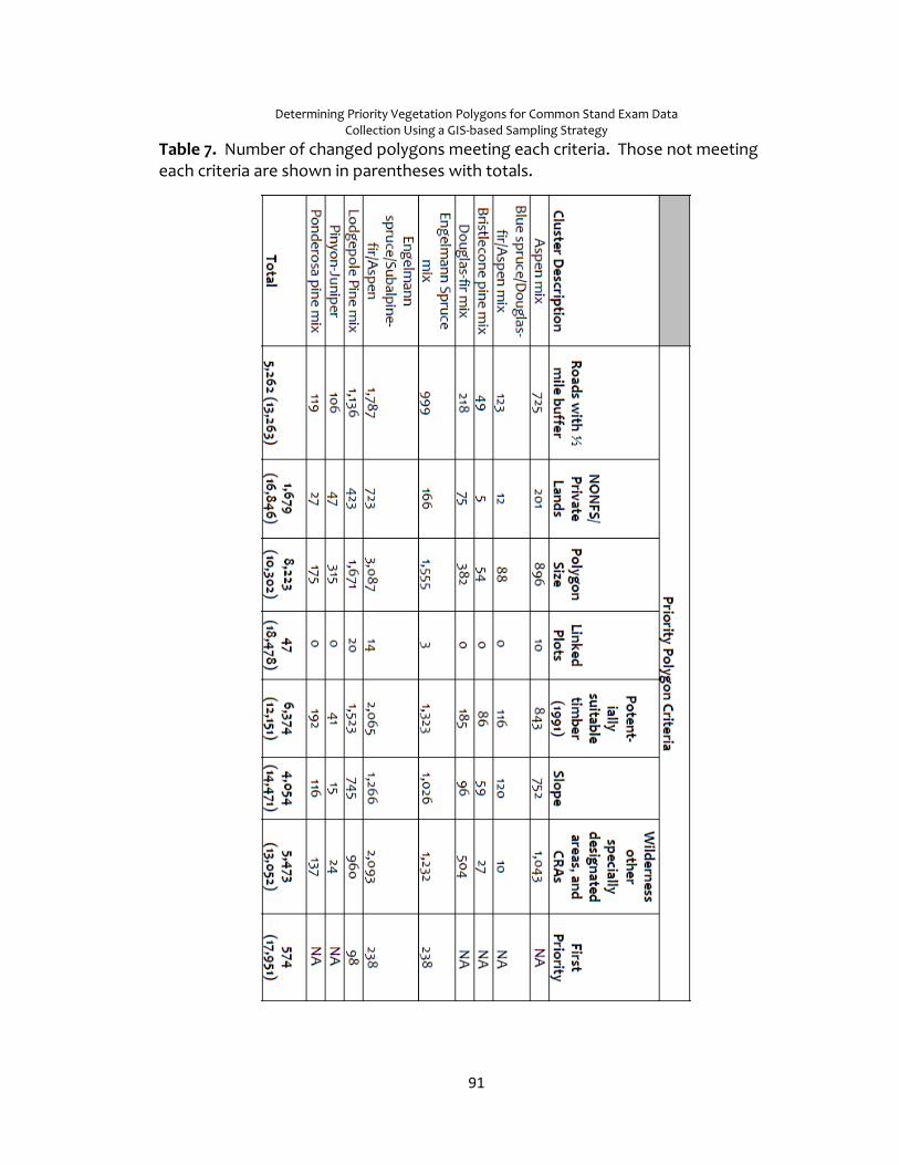
Determining Priority Vegetation Polygons for Common Stand Exam Data Collection Using a GIS-based Sampling Strategy
91
Table 7. Number of changed polygons meeting each criteria. Those not meeting each criteria are shown in parentheses with totals.

Determining Priority Vegetation Polygons for Common Stand Exam Data Collection Using a GIS-based Sampling Strategy
92
Overlaying First Priority Polygons with Vegetation Altering Activities The first priority polygons remaining from the intersection with the VAA layer
resulted in only 254 polygons. Upon closer examination of the VAA intersection with
first priority polygon selection, many polygons were only touching the boundaries of
VAAs or the edges of polygons were only slightly affected by VAAs (Figure 20).
Therefore, this intersection was ignored and I performed another intersection with
Figure 20. Example of VAA intersection with priority polygons whereby VAAs touch the boundaries of three priority polygons and have only affected a minute percentage of the polygons’ area.
VAAs once all three prioritized polygon selections were made and the three
selections were merged into one feature class.
Second and Third Priority Polygon Selections The second priority polygon sampling model produced 472 second priority polygons.
Only nine polygons returned as satisfying the criteria to be third priority.

Determining Priority Vegetation Polygons for Common Stand Exam Data Collection Using a GIS-based Sampling Strategy
93
Determination of Final Priority Polygons
Final Priority Polygons with VAAs I merged first, second, and third priority polygons together into one feature class
resulting in 1055 polygons within the merged feature class. When I performed a
selection by location using the merged polygons and VAA feature class, 49% or 518
polygons intersected with VAAs. Upon further review of the intersection, I
discovered that 636 polygons not to be significantly affected by VAAs. Those 636
polygons were deemed priority polygons to go onto the final stage of review for field
data collection.
Final Selection of Priority Polygons After several iterations of review by the SO timber staff, SO GIS staff, and Gunnison
RD silviculturist, they determined that 462 out of the 636 polygons would be the final
polygons to be visited in the field for CSE data collection. The reduction was mainly a
result of two different issues: 1) access limitations, and 2) CSE data already existing
for many polygons but still unlinked. That is, many of the polygons excluded from
field data collection consideration as a result from the final review process already
had plot data collected from them; however, the data for these polygons had not
been linked to the polygons in FSVeg Spatial, thereby giving no indication that CSE
data had been collected for these polygons. Furthermore, I was not provided this
information until after completing the GIS sampling exercises and I had given the
priority polygons to timber staff for final review. As a result of the review, 174
additional polygons were excluded from field data collection. Overall, priority
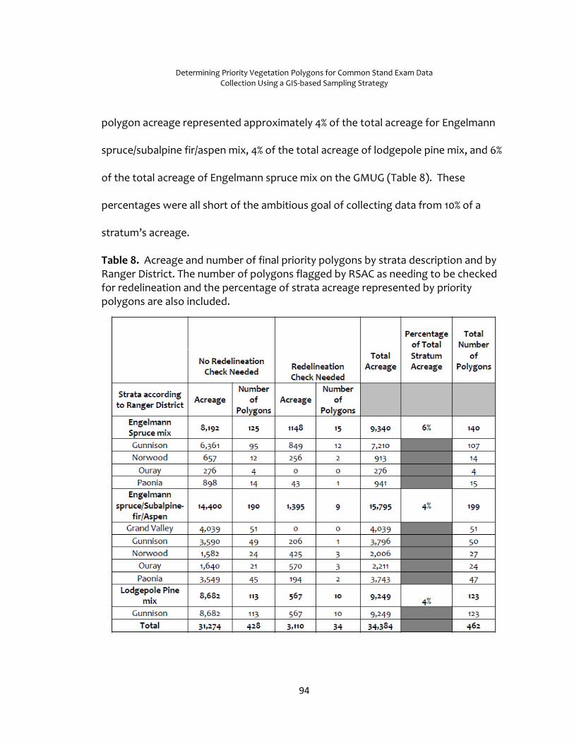
Determining Priority Vegetation Polygons for Common Stand Exam Data Collection Using a GIS-based Sampling Strategy
94
polygon acreage represented approximately 4% of the total acreage for Engelmann
spruce/subalpine fir/aspen mix, 4% of the total acreage of lodgepole pine mix, and 6%
of the total acreage of Engelmann spruce mix on the GMUG (Table 8). These
percentages were all short of the ambitious goal of collecting data from 10% of a
stratum’s acreage.
Table 8. Acreage and number of final priority polygons by strata description and by Ranger District. The number of polygons flagged by RSAC as needing to be checked for redelineation and the percentage of strata acreage represented by priority polygons are also included.

Determining Priority Vegetation Polygons for Common Stand Exam Data Collection Using a GIS-based Sampling Strategy
95
4.4 Phase IV
4.4.1 Polygon Redelineation Only those polygons selected as final priority polygons from the sampling strategy
were redelineated in Phase IV. There were a total of 1236 polygons from all nine
strata that had been flagged by RSAC as possibly needing redelineation. Only 34 out
of those 1236 polygons were selected as final priority polygons. I reshaped four of
those 34 before plot layout. Three of the four redelineations comprised of only
moving boundaries to match obvious breaks in the tree stand (Figure 21). One
Figure 21. Slight modification in polygon boundary considered as a redelineation. Yellow line indicates redelineated boundary and black line represents old polygon boundary.
delineation was performed because polygon was not displaying homogeneous
conditions.

Determining Priority Vegetation Polygons for Common Stand Exam Data Collection Using a GIS-based Sampling Strategy
96
On the other hand, the Gunnison RD polygons selected for field data collection were
redelineated based on the review and at the discretion of the Gunnison RD
silviculturist. He redelineated 207 polygons although only 23 polygons were flagged
for redelineation by RSAC (Table 9). He split several of these polygons into smaller
ones based upon the stand characteristics found in the field. After reviewing his
delineations, I determined that the editor would have to have intimate field
knowledge of these polygons in order to come up with some of these same
redelineations as I had a difficult time in determining from imagery how the location
of boundaries were decided upon.
FSVeg Spatial protocols allow for subjectivity in polygon delineations and with any
FSVeg Spatial edits, lumping or splitting of polygons is at the discretion of the editor.
The silviculturist ended up creating sixteen new polygons: six new polygons in the
Engelmann Spruce mix, one in Engelmann spruce/subalpine-fir/aspen mix, and nine in
the Lodgepole pine mix. These new polygons were a consequence of splitting
several polygons to produce more homogeneous stand conditions than previous
delineations (Figure 22).

Determining Priority Vegetation Polygons for Common Stand Exam Data Collection Using a GIS-based Sampling Strategy
97
Figure 22. Result of splitting a large polygon (in black) into several smaller polygons (in yellow). This image shows a split of one lodgepole pine mix polygon into three separate polygons. Yellow line designates new polygon delineations and black line displays old polygon boundaries.
In other cases, the silviculturist edited polygon boundaries to match the edge of tree
stands as seen with NAIP or resource imagery. A majority of the delineation changes
were a result of viewing polygons with newer and higher resolution imagery as
compared to the imagery that was used in original delineations. When viewed with
the polygon boundaries, the more recent imagery showed where boundaries could
be edited to more accurately reflect divisions and changes in vegetation type and
condition and better demarcate edges of tree stands.

Determining Priority Vegetation Polygons for Common Stand Exam Data Collection Using a GIS-based Sampling Strategy
98
Table 9. Priority polygons on Gunnison RD redelineated by silviculturist
Strata
Total Polygons per Strata
Not Flagged by RSAC
Redelineated by
Silviculturist Flagged by
RSAC
Engelmann Spruce mix 107 95 70 12
Engelmann spruce/subalpine-
fir/aspen 50 49 34 1
Lodgepole Pine mix 123 113 103 10
Total 280 257 207 23
4.4.2 Plot Layout and Contract Maps After polygon redelineation, both the silviculturist and I performed plot layout. The
silviculturist laid out 1,511 plots in 280 polygons that resided on the Gunnison RD. I
laid out 1,328 plots in 182 polygons residing on the other four districts. Therefore,
the contract maps consisted of a total of 2,839 plots that went out for bid (Figures 23
and 24 and Appendix B, Figures B3-B10 for polygon/strata overview maps).
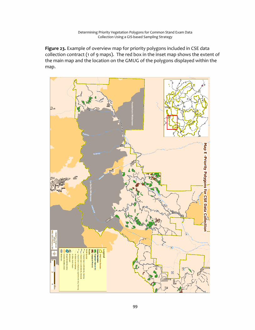
Determining Priority Vegetation Polygons for Common Stand Exam Data Collection Using a GIS-based Sampling Strategy
99
Figure 23. Example of overview map for priority polygons included in CSE data collection contract (1 of 9 maps). The red box in the inset map shows the extent of the main map and the location on the GMUG of the polygons displayed within the map.

Determining Priority Vegetation Polygons for Common Stand Exam Data Collection Using a GIS-based Sampling Strategy
100
Figure 24. Example of a data driven map for CSE data collection contract. Each map shows one polygon. For this reason, there are 462 maps included in the contract.

Determining Priority Vegetation Polygons for Common Stand Exam Data Collection Using a GIS-based Sampling Strategy
101
Chapter Five
Discussion In this chapter, I have provided some insight on model building and discussed several
issues ranging from geoprocessing results to data maintenance that arose during the
Practicum. I have divided discussion into subsections based on the issue addressed.
5.1 High Complexity I completed the steps needed to address my research questions by creating tools
with attributes in Allen (2011) and similar to the ones discussed in Lin et al. 2006.
Although the ability to rerun is inherent with a tool built in ModelBuilder, I would
argue that it is this inherent capability that makes a tool quite useful and effective.
This project’s tools allowed steps to be run multiple times to produce several
different derived alternatives. Secondly, the selection of priority polygons required
the incorporation of several different datasets and many of the datasets required
further querying to identify the subset of data needed for priority polygon selection.
Being able to use the same geoprocessing workflows documented in the tools when
needed allowed me to be more efficient in obtaining results by not having to recreate
geoprocessing steps each time before performing subsequent analyses. Also, the
reuse of tools proved valuable in double checking geoprocessing results and
comparing results after I had modified or queried input datasets.
The amount of datasets involved in the analyses added complexity to the model
building. Tang et al. 2014 also had a large number of GIS functions and tools involved

Determining Priority Vegetation Polygons for Common Stand Exam Data Collection Using a GIS-based Sampling Strategy
102
in his model for building LiDAR derived hydrologic feature datasets. Like Tang et al.
2014, I was able to simplify how the analyses were performed through the use of
ModelBuilder and with this use was able to reduce processing time. Furthermore, I
would not have maintained consistency in data analysis if I had manually repeated all
geoprocessing steps each time I needed to do so. Instead, I was able to automate
and repeat all geoprocessing steps as well as reference the workflow documentation
at any time during the project through tool creation and utilization. Overall, I was
able to reduce inefficiency and maintain consistency in data analysis by producing
and using tools for this project.
On the other hand, tools can be difficult to rerun with success if during the building
phase of the tool, the designer is unskilled in constructing the tools using the many
options and functions of ModelBuilder. For example, I was unskilled in writing and
using Python script when building the tools for this project. If I had incorporated if-
elif-else controls using Python script into the tools, I probably would have made the
tools more efficient to reuse in some aspects (Allen 2011). Within an if-elif-else
control, a Stop tool evaluates an input Boolean value and can cue the model to either
stop running or continue with another process, depending on the value. One simple
way of improving the first priority polygon sampling tool could have been to write an
if-elif-else control to direct the tool to check if certain fields had been deleted prior to
the tool being fully executed again. I would forget many times to delete fields added

Determining Priority Vegetation Polygons for Common Stand Exam Data Collection Using a GIS-based Sampling Strategy
103
and calculated from the tool before rerunning the tool, which would cause problems
in subsequent tool execution. Originally, to address this issue, I added the Delete
Field tool into the first priority polygon sampling tool to delete fields from the
Polyselection1 feature class if those fields existed in the feature class prior to the tool
re-adding and recalculating the same fields. Unfortunately, however, with the
incorporation of the Delete Field tool, a schema lock would occur each time I reran
the tool. For this reason, I decided not to use it and removed the Delete Field tool
from the first priority polygon tool. The incorporation of the Python script control
may not have prevented the schema lock from occurring but it would remind me to
manually delete fields before the tool could be re-executed. This would prevent
committing further errors when running the polygon tool multiple times.
5.2 Cost I selected $100 per plot estimate for field data collection used in this project because
the SO timber staff’s plan was to have the majority if not all of the CSE data collection
on the GMUG covered by IDIQ contract. Costs for past CSE data collection via IDIQ
contract had been a little under $100 per plot. Unfortunately, due to issues with
contracting, only a TEAMS unit could be contracted for the summer of 2016 and its
costs of field data collection per plot were much higher than that under an IDIQ
contract. For this reason, data collection costs for the tree mortality update project
were much more than originally forecasted. However, a second contract for 2017
CSE data collection will be made in the winter and spring of 2017. The hope is that an
Determining Priority Vegetation Polygons for Common Stand Exam Data Collection Using a GIS-based Sampling Strategy
104
IDIQ contract can be awarded and per plot costs for 2017 CSE data collection will be
much lower than the 2016 costs.
Due to limited funds for project implementation, the GMUG decided to limit field
collection to only three out of nine strata and update records of tree species only
found within those three strata. The decision to focus on three of nine strata
revolved around availability of funds. However, the choice of the three strata to
focus on in the update process for the GMUG was based largely on aerial detection
survey data (ADS) and other field observations. These surveys and observations
showed that a large portion of Engelmann spruce, subalpine fir, aspen, and
lodgepole pine tree populations on the GMUG had died over the last twenty years
mostly as a result of bark beetle infestations and factors of SAD (US Forest Service,
2016a, Worrall et al. 2010, Marchetti et al. 2011). NDVI analysis results presented in
this Practicum agreed with these findings as a majority of change in NDVI on the
GMUG was found within the Engelmann spruce mix, Engelmann spruce/subalpine-
fir/aspen mix, and lodgepole pine mix strata. The stratum showing the fourth largest
change in NDVI was aspen mix.
Although the GMUG decided to fund CSE data collection for 2,839 plots within 462
polygons belonging to three different strata, the RGNF funded field data collection
for 2,630 plots within 335 polygons belonging to all eleven strata found on the Forest
(Stam et al. 2016). This data collection updated FSVeg Spatial records for all tree

Determining Priority Vegetation Polygons for Common Stand Exam Data Collection Using a GIS-based Sampling Strategy
105
species found on the RGNF. If GMUG funds field data collection for all 462 polygons
at the same plot sampling intensity utilized in the 2016 CSE data collection contract,
tree mortality rates for GMUG may be more accurate than those calculated for the
RGNF due the GMUG having a larger sample size representative of each strata as
compared to the RGNF.
5.3 Use of NDVI Data Compared to Aerial Detection Survey Data I originally utilized insect and disease infestation activity polygons obtained from
ADS, conducted by Forest Health Protection and its partners, in this analysis to
determine what vegetation polygons on the GMUG had been affected by these
pathogens. After consultation with RSAC, I used low NDVI year raster produced by
RSAC in hopes to better inform GMUG timber and planning staff as to which recently
collected linked and unlinked plot data may still be potentially valid and be used in
mortality rate calculations for the change detection project. Low NDVI year raster
provided a two year range for each pixel on the GMUG when the lowest NDVI (least
green) was detected. The number and location of plots obtained by using this data
layer was similar but not identical to that obtained by ADS data. 120 more plots
resulted from the use of the low NDVI year raster layer rather than ADS data in the
linked plot model. Using ADS data would have yielded a more conservative number
of plots potentially valid for mortality rate calculations. In conclusion, the raster layer
was not necessarily a superior data source than the ADS data in showing where
change from pathogens could and have taken place on the GMUG. Instead, RSAC
Determining Priority Vegetation Polygons for Common Stand Exam Data Collection Using a GIS-based Sampling Strategy
106
preferred the GMUG to use the low NDVI year data source over ADS data for
determining previously collected plot data that potentially could be used in mortality
rate calculations. This preference stemmed from the fact that ADS is subjective in
nature, with no two sketchmappers producing the same mapping results (Klein et al.
1983) (see Appendix A, A.2 Role of Field Collected Data, Aerial Detection Survey Data,
and Remotely Sensed Data for more discussion on this topic). Furthermore, RSAC
regards the use of the raster layer compared to that of ADS data to be a more
objective and consistent approach in deciding which plots to accept and include in
mortality rate calculations.
5.4 FSVeg Spatial Discrepancies
5.4.1 Polygons In Need of Redelineation I noticed several discrepancies with data maintenance in FSVeg Spatial while
performing analyses for this project. One is that some polygons that had undergone
some sort of vegetation altering treatment had not been redelineated in FSVeg
Spatial after treatment implementation to reflect a change in stand conditions. Also,
I had learned that many polygons on the Gunnison RD had been reshaped by the
silviculturist in the last several years. However, he had not entered these edits into
FSVeg Spatial yet. These issues bring to light that a more thorough examination of
polygons needs to occur prior to the update algorithm being applied in order to catch
discrepancies like these before any polygon record changes take place by the
automated update. If polygons such as these are included in the algorithm update,

Determining Priority Vegetation Polygons for Common Stand Exam Data Collection Using a GIS-based Sampling Strategy
107
polygon inaccuracies such as these will just be proliferated rather than addressed and
fixed.
5.4.2 Inaccurate Species Compositions for Some Polygons The GIS shop plans on conducting ongoing discussions and making a coordinated
effort with the GMUG timber staff to update forested polygons intentionally left out
of the automated update and those not yet known to have inaccurate species
compositions. This will require close collaboration with timber personnel to identify
and edit these polygons in FSVeg Spatial with correct attribute information as
determined from field visits or using foresters’ and silviculturists’ extensive field
knowledge of these areas. These tasks will take place over time but completing this
work in a timely manner should be goal for the GMUG so as to address and fix these
data discrepancies sooner rather than later.
5.4.2 Linked and Unlinked Plots I reviewed priority polygons within the west and east timber zone planning areas (7N,
Long Creek, Moore-Payne, and Transfer on the Uncompahgre Plateau of the Ouray
RD and in areas around Kebler Pass and north of Taylor Park on the Gunnison RD) to
determine which polygons data had already been collected. This data collection
effort was separate from that for the mortality update project. Contract and agency
timber crews had collected data from these areas prior to 2016 or during the summer
of 2016 for timber sale preparation. Although the data were not originally collected
for the purpose of calculating mortality rates, timber staff agreed that it would serve
Determining Priority Vegetation Polygons for Common Stand Exam Data Collection Using a GIS-based Sampling Strategy
108
a dual purpose, if possible, to be used for timber sale preparation and in the mortality
update process. Unfortunately, most plot data had not been linked to polygons in
FSVeg Spatial. As a result of not maintaining plot data in FSVeg Spatial by archiving
old plot data and linking newly collected plot data, many of the plots generated from
recent data collection efforts were not and are not found in FSVeg Spatial.
Therefore, this plot data were not included in the base dataset used by the linked
plot tool to determine potentially valid plots. I will be making an extensive effort
during the 2017 winter to link most recent plot data to corresponding polygons for
project areas where this has not been already done in FSVeg Spatial. Once the
linkage is complete, I will gather and finalize all plot data that potentially can be used
in mortality rate calculations to be delivered to the SO timber staff for final review.
5.5 Relationship Criteria When I examined the result from the first priority polygon sampling tool, I found
several polygons not to be completely within the ½ mile road buffer. I had designed
the tool to select those polygons that intersected any ½ mile road buffer. When I
chose “completely within” (polygons completely within the road buffer) rather than
“intersect” for the relationship type, only 251 of the 574 first priority polygons
resulted and met the selection criterion. Also, I discovered that 36 of 574 polygons
had a majority of their area in unsuitable timber areas and only small areas
intersecting suitable timber areas. This occurrence took place because I chose
‘intersect’ rather than “have their centroid in” as the relationship type for the

Determining Priority Vegetation Polygons for Common Stand Exam Data Collection Using a GIS-based Sampling Strategy
109
selecting criterion. When I switched the relationship type to “have their centroid in”,
499 polygons met the criterion of having a majority of their area as potentially
suitable for commercial timber harvest. Lastly, I did not include proximity of
polygons to large towns as a final determining factor for priority. I did perform a
selection by location to select first priority polygons that were within 20 miles of a
town to see how many priority polygons met this criterion. 448 of 574 polygons
matched this criteria. Because the proximity is based on as the “crow flies” distance
between two locations, I contemplated performing a least cost path analysis to more
accurately determine the route wise distance from a polygon to a town. I would
have then applied route length calculations to select those polygons that were
closest or had the most cost-effective route to town or to an agency office.
However, after discussion with the SO timber and GIS staff about the usefulness of
the analysis, they decided the greater complexity provided by the analysis was not
warranted.
5.6 Conclusions I successfully addressed the seven research questions raised in this Practicum and
fully answered five of the seven questions (refer to section 1.3). The last two
questions regarding recent and valid CSE data is still in the process of being fully
answered. I have described future work to complete in addressing these two

Determining Priority Vegetation Polygons for Common Stand Exam Data Collection Using a GIS-based Sampling Strategy
110
questions and in helping with the completion of future supervised delineation and
attribute updates to vegetation polygons.
5.6.1 Future Work Because this work was unable to be finished during the timeframe of the Practicum,
Carol Howe, Resource Information Specialist for the GMUG, and I will be completing
any needed redelineations starting in the winter of 2017. We will start with those
flagged by RSAC but will also include in the review those polygons needing minor
edits. Minor edits entail those arising from differences in imagery used in the original
delineation efforts compared to newer imagery used to perform current
redelineations.
Many vegetation polygons will not be updated using the automated algorithm,
mainly due not collecting field data for nonpriority strata. Therefore, supervised
attribute edits for polygons not included in the algorithm update will need to occur
even after the completion of this Practicum. One way to manage the execution of
needed edits would be to prioritize the excluded polygons from this Practicum’s
work and utilize those priority designations to direct future work involving spatial
redelineations and supervised attribute updates.
Archiving old plot data in FSVeg and FSVeg Spatial and linking valid plot data in FSVeg
Spatial will be also an important task to complete winter of 2017. Old plot data is
data that have been collected in the distant past and no longer quantify existing
conditions. Once old plot data is archived, recently collected plot data can be linked

Determining Priority Vegetation Polygons for Common Stand Exam Data Collection Using a GIS-based Sampling Strategy
111
in FSVeg Spatial. The completion of this particular task will be instrumental in
increasing the amount of data made available for mortality rate calculations.
Furthermore, increasing the amount of field data used in calculations should improve
the accuracy of mortality rates.
GIS staff are aware of general locations of some polygons with inaccurate species
compositions. However, exact Setting IDs which are unique identifications for
polygons still need to be identified for exclusion from the automated update. The
attributes of these polygons will need to be updated manually in FSVeg Spatial either
after plot data has been collected or the FSVeg Walkthrough Form (refer to Figure 3)
has been completed as a result of field visits.
In addition to providing information regarding mortality within polygons, plot data
will also aid in updating other stand attributes than just the percentage of dead. GIS
staff will use a newly created FSVeg Spatial tool that applies plot data in calculating
tree cover percentages of all species, both live and dead percentages, found within
the plots of a polygon. Additionally, attributes listed in the FSVeg Spatial
Walkthrough Form will also be updated for every polygon included in the contract.
The data collected on the form will be incorporated into the FSVeg Spatial database
using a database loader tool.
Lastly, I and others in the GMUG GIS shop plan on developing 3D photo
interpretation skills using a new stereo viewing software extension Summit Evolution

Determining Priority Vegetation Polygons for Common Stand Exam Data Collection Using a GIS-based Sampling Strategy
112
which recently started being used by the USFS in the spring of 2016 to test out its
efficiency in stereo viewing as compared to Stereo Analyst. If it proves to be quicker
in downloading and processing image files, we, the GMUG GIS shop, will use Summit
Evolution extension to more clearly detect differences in stand structure and species
composition among vegetation polygons.
5.6.2 Management Implications Work performed for this Practicum placed emphasis on : 1) the need for consistent
and accurate field data collection across the GMUG, following all FSVeg Spatial and
FSVeg protocols for data collection, 2) the importance of updating polygon
delineations and attributes in the FSVeg Spatial database annually, 3) training
individuals in FSVeg Spatial and FSVeg to be able to correctly and accurately update
structure and composition of forested polygons, and lastly, 4) tasking those trained
individuals with the responsibility of making FSVeg Spatial and FSVeg updates on a
consistent basis.
5.6.3 Final Remarks Overall, the work performed in this Practicum successfully selected vegetation
polygons from which field data was and will be collected based on several criteria
implemented in a GIS sampling strategy. The criteria helped reduce per plot cost and
maximize the number of plots for field data collection keeping in mind the budget
allocated to this task. Vegetation polygons will be updated once the tree mortality

Determining Priority Vegetation Polygons for Common Stand Exam Data Collection Using a GIS-based Sampling Strategy
113
rule sets are developed from the collected plot data. Once the updates have taken
place, FSVeg Spatial records will be more accurate in reflecting existing conditions for
forested polygons, rather than conditions from more than 25 years ago. These
conditions can then be used to revise the FLMP to provide better guidance in
managing the natural resources on the three Forests. A revised and more current
FLMP will allow the Forests to be more accountable to the citizens of the United
States for the purpose to which the agency was originally created, “Caring for the
Land and Serving the People”.

Determining Priority Vegetation Polygons for Common Stand Exam Data Collection Using a GIS-based Sampling Strategy
114
References
Allen, D. W. (2011). Getting to know ArcGIS ModelBuilder (1st ed.). Redlands, CA: Esri Press.
Anderegg, L. D. L., Anderegg, W. R. L., Abatzoglou, J., Hausladen, A. M., & Berry, J. A. (2013). Drought characteristics' role in widespread aspen forest mortality across Colorado, USA. Global Change Biology, 19(5), 1526-1537. doi:10.1111/gcb.12146
Andrew, M. E., Wulder, M. A., & Nelson, T. A. (2014). Potential contributions of remote sensing to ecosystem service assessments. Progress in Physical Geography, 38(3), 328-353. doi:10.1177/0309|333|4528942
Bellante, G., Goetz, W., Maus, P., Wittwer, D., Schrader, B., Johnson, E., Megown, K. (2015). Yakutat foreland existing vegetation map project. (No. RSAC-10106-RPT1). Salt Lake City, Utah: United Stated Department of Agriculture, Forest Service, Remote Sensing Applications Center.
Bentz, B. J., Régnière, J., Fettig, C. J., Hansen, E. M., Hayes, J. L., Hicke, J. A., . . . Seybold, S. J. (2010). Climate change and bark beetles of the western United States and Canada: Direct and indirect effects. Bioscience, 60(8), 602-613. doi:10.1525/bio.2010.60.8.6
Biswas, T., Heutte, T., Riley, M., Wittwer, D. T., Maus, P, Megown, K. (2016). A Landsat method to monitor aspen defoliation southwest of Fairbanks, interior Alaska. ( No. RSAC-10116-RPT1). Salt Lake City, Utah: United Stated Department of Agriculture, Forest Service, Remote Sensing Applications Center.
Campbell, J. B., & Wynne, R. H. (2011). Introduction to Remote Sensing (5th ed.). New York, NY: The Guilford Press.
Chi, G. (2010). Land developability: Developing an index of land use and development for population research. Journal of Maps, 609-617. doi:10.4113/jom.2010.1146
Code of Federal Regulations (2015a). Title 36: Parks, Forests, Public Property. Chapter 2: Forest Service, Department of Agriculture. 212: Travel Management. https://www.law.cornell.edu/cfr/text/36/part-212.
Code of Federal Regulations (2015b). Title 36: Parks, Forests, Public Property. Chapter 2: Forest Service, Department of Agriculture. 251: Land Uses. https://www.law.cornell.edu/cfr/text/36/part-251

Determining Priority Vegetation Polygons for Common Stand Exam Data Collection Using a GIS-based Sampling Strategy
115
Code of Federal Regulations (2015c). Title 36: Parks, Forests, Public Property. Chapter 2: Forest Service, Department of Agriculture. 261: Prohibitions. https://www.law.cornell.edu/cfr/text/36/part-261
Coelho, A. C., Labadie, J. W., & Fontane, D. G. (2012). Multicriteria decision support system for regionalization of integrated water resources management. Water Resource Management, 26, 1325-1346.
Cohen, W. B., & Goward, S. N. (2004). Landsat's role in ecological applications of remote sensing. Bioscience, 54(6), 535-545.
Collins, J. B., & Woodcock, C. E. (1996). An assessment of several linear change detection techniques for mapping forest mortality using multi-temporal Landsat TM data. Remote Sensing of Environment, 56, 66-77.
Coops, N. C., Johnson, M., Wulder, M. A., & White, J. C. (2006). Assessment of QuickBird high spatial resolution imagery to detect red attack damage due to mountain pine beetle. Remote Sensing of Environment, 103, 67-80. doi:10.1016/j.rse.2006.03.012
Coppin, P., Jonckheere, I., Nackaerts, K., & Muys, B. (2004). Digital change detection methods in ecosystem monitoring: A review. International Journal of Remote Sensing, 25(8), 1565-1596. doi:10.1080/0143116031000101675
Deng, J. S., Wang, K., Deng, Y. H., & Qi, G. J. (2008). PCA-based land-use change detection and analysis using multi-temporal and multisensor satellite data. International Journal of Remote Sensing, 29(16), 4823-4838. doi:10.1080/01431160801950162
ESRI. (2016). What is ModelBuilder?-Help|ArcGIS for desktop. Retrieved from http://desktop.arcgis.com/en/arcmap/10.3/analyze/modelbuilder/what-is-modelbuilder.htm
Gardiner, T. (2015). In Kolanoski K. (Ed.), Tree mortality around Ouray, Colorado and bark beetle effects on Uncompahgre Plateau.
Goodwin, N. R., Coops, N. C., Wulder, M. A., Gillanders, S., Schroeder, T. A., & Nelson, T. (2008). Estimation of insect infestation dynamics using a temporal sequence of Landsat data. Remote Sensing of Environment, 112, 3680-3689. doi:10.1016/j.rse.2008.05.005

Determining Priority Vegetation Polygons for Common Stand Exam Data Collection Using a GIS-based Sampling Strategy
116
Hansen, E. M., Negron, J. F., Munson, A. S., & Anhold, J. A. (2010). A retrospective assessment of partial cutting to reduce spruce beetle-caused mortality in the southern Rocky Mountains. Western Journal of Applied Forestry, 25(2), 81-87.
Hebertson, E. G., & Jenkins, M. J. (2008). Climate factors associated with historic spruce beetle (Coleoptera:Curculionidae) outbreaks in Utah and Colorado. Environmental Entomology, 37(2), 281-292.
Hsu, W. C., Remar, A., Williams, E., McClure, A., Kannan, S., Steers, R., Schmidt, C., & Skiles, J. W. (2012). The changing California coast: Relationships between climatic variables and coastal vegetation succession. ASPRS 2012 Annual Conference, March 19-23, Sacramento, California. 12 p.
Ireland, K. B., Moore, M. M., Fulé, P., Zegler, T. J., & Keane, R. E. (2014). Slow lifelong growth predisposes Populus tremuloides trees to mortality. Oecologia, 175, 847-859. doi:10.10077/s00442-014-2951-5
Kelly, M., & Di Tommaso, S. (2015), Mapping forest with LiDAR provides flexibility, accurate data with many uses. California Agriculture, 69, 14-20. doi:10.3733/ca.v069n01p14
Kennedy, R. E., Cohen, W. B., & Schroeder, T. A. (2007). Trajectory-based change detection for automated characterization of forest disturbance dynamics. Remote Sensing of Environment, 110, 370-386. doi:10.1016/j.rse.2007.03.010
Klein, W. H., Tunnock, S., Ward, J. G. D., & Knopf, J. A. E. (1983). Aerial Sketchmapping. In: Forest Insect and Disease Survey Methods Manual. Davis, California: USDA Forest Service, Forest Pest Management, Methods Application Group, 15 pp.
Knorn, J., Rabe, A., Radeloff, V. C., Kuemmerle, T., Kozak, J., & Hostert, P. (2009). Land cover mapping of large areas using chain classification of neighboring Landsat satellite images. Remote Sensing of Environment, 113, 957-964. doi:10.1016/j.rse.2009.01.010
Kuhmaier, M., & Stampfer, K. (2010). Development of a multi-attribute spatial decision support system in selecting timber harvesting systems. Croatian Journal of Forest Engineering, 31(2), 75-88.
Lillesand, T. M., Kiefer, R. W., & Chipman, J. W. (2004). In Flahive R., Powell D. (Eds.), Remote sensing and image interpretation (5th ed.). New York, NY: John Wiley & Sons, Inc.

Determining Priority Vegetation Polygons for Common Stand Exam Data Collection Using a GIS-based Sampling Strategy
117
Linn, J. P., Bourne, S. G., & Kleiss, B. A. (2006). Creating a wetland restoration decision support system using GIS tools. ( No. ERDC TN-EMRRP-EM-05). Vicksburg, MS: U.S. Army Engineer Research and Development Center. doi:http://el.erdc.usace.army.mil/emrrp/emrrp.html
Lunetta, R. S., Knight, J. F., Ediriwickrema, J., Lyon, J. G., & Worthy, L. D. (2006). Land-cover change detection using multi-temporal MODIS NDVI data. Remote Sensing of Environment, 105(2), 142-154. doi:10.1016/j.rse.2006.06.018
Marchetti, S. B., Worrall, J. J., & Eager, T. (2011). Secondary insects and diseases contribute to sudden aspen decline in southwestern Colorado, USA. Canadian Journal of Forest Resources, 41, 2315-2325. doi:10.1139/X11-106
Mayer, A. L., & Lopez, R. D. (2011). Use of remote sensing to support forest and wetlands policies in the USA. Remote Sensing, 3(6), 1211-1233. doi:10.3390/rs3061211
McRoberts, R. E., Cohen, W. B., Naesset, E., Stehman, S. V., & Tomppo, E. O. (2010). Using remotely sensed data to construct and assess forest attribute maps and related spatial products. Scandinavian Journal of Forest Research, 25, 340-367. doi:10.1080/02827581.2010.497496
Meddens, A. J. H., & Hicke, J. A. (2014). Spatial and temporal patterns of Landsat-based detection of tree mortality caused by mountain pine beetle outbreak in Colorado, USA. Forest Ecology and Management, 322, 78-88. doi:10.1016/j.foreco.2014.02.037
Meddens, A. J. H., Hicke, J. A., & Vierling, L. A. (2011). Evaluating the potential of multispectral imagery to map multiple stages of tree mortality. Remote Sensing of Environment, 115, 1632-1642. doi:10.1016/j.rse.2011.02.018
Meigs, G. W., Kennedy, R. E., & Cohen, W. B. (2011). A Landsat time series approach to characterize bark beetle and defoliator impacts on tree mortality and surface fuels in conifer forests. Remote Sensing of Environment, 115, 3707-3718. doi:10.1016/j.rse.2011.09.009
Michaelian, M., Hogg, E. H., Hall, R. J., & Arsenault, E. (2011). Massive mortality of aspen following severe drought along the southern edge of the Canadian boreal forest. Global Change Biology, 17, 2084-2094. doi:10.1111/j.1365-2486.2010.02357.x

Determining Priority Vegetation Polygons for Common Stand Exam Data Collection Using a GIS-based Sampling Strategy
118
Mitchell, B., Beaty, M., Reynolds, R., Mellin, T., Hudak, A.T., Schaaf, A., Fisk, H. (2015). Creating LiDAR Canopy Structure Layers and inventory models for evaluating northern goshawk habitat quality ( No. RSAC-10070-RPT1). Salt Lake City, Utah: United Stated Department of Agriculture, Forest Service, Remote Sensing Applications Center.
Moffiet, T., Mengersen, K., Witte, C., King, R., & Denham, R. (2005). Airborne laser scanning; exploratory data analysis indicates potential variables for classification of individual trees or forest stands according to species. ISPRS Journal of Photogrammetry and Remote Sensing, 59, 289-309. doi:10.1016/j.isprsjprs.2005.05.002
Mueller, R. C., Scudder, C. M., Porter, M. E., Trotter III, R. T., Gehring, C. A., & Whitham, T. G. (2005). Differential tree mortality in response to severe drought: Evidence for long-term vegetation shifts. Journal of Ecology, 93(6), 1085-1093. doi:10.1111/j.1365-2745.2005.01042.x
Mustian, A. P. (1978). History and philosophy of silviculture and management systems in use today. Uneven-Aged Silviculture and Management in the Western United States, Redding, California. 1-10.
Pasual, C., Garcia-Montero, L. G., Arroyo, L. A., & Garcia-Abril, A. (2013). Increasing the use of expert opinion in forest characterization approaches based on LiDAR data. Annals of Forest Science, 70, 87-99. doi:10.1007/s13595-012-0232-1
Potter, C. (2015). Changes in vegetation cover and productivity in Yosemite national park (California) detected using Landsat satellite image analysis. Journal of Biodiversity Management and Forestry, 4(4) doi: http://dx.doi.org/10.4172/2327-
4417.1000148
Rebain, S. (2016). Logic used to create a GIS model to estimate suitable timber acres. Unpublished manuscript.
Rehfeldt, G., Worrall, J., Marchetti, S., & Crookston, N. (2015). Adapting forest management to climate change using bioclimate models with topographic drivers. Forestry, 0(February), 1-12. doi:10.1093/forestry/cpv019
Singh, A. (1989). Digital change detection techniques using remotely-sensed data. International Journal of Remote Sensing, 10(6), 989-1003. doi:10.1080/01431168908903939
Determining Priority Vegetation Polygons for Common Stand Exam Data Collection Using a GIS-based Sampling Strategy
119
Skakun, R. S., Wulder, M. A., & Franklin, S. E. (2003). Sensitivity of the thematic mapper enhanced wetness difference index to detect mountain pine beetle red-attack damage. Remote Sensing of Environment, 86, 433-443. doi:10.1016/S0034-4257(03)00112-3
Smith, D. M., Larson, B. C., Kelty, M. J., & Ashton, P. M. S. (1997). In Stano E. (Ed.), The Practice of Silviculture: Applied Forest Ecology (9th ed.). Hoboken, N.J.: John Wiley & Sons, Inc.
Stam, C., Goetz, W., Maus, P., Dressen, M., Zwisler, S., Caulkins, J., & Megown, K. (2015a). Medicine Bow-Routt National Forest: FSVeg database update. ( No. RSAC-10095-RPT1). Salt Lake City, Utah: United States Department of Agriculture, Forest Service, Remote Sensing Applications Center.
Stam, C., Goetz, W., Megown, K., Dressen, M., & Zwisler, S. (2015b). Forest-wide mortality statistics: Using common stand exam data. ( No. RSAC-10095-Brief1). Salt Lake City, Utah: United Stated Department of Agriculture, Forest Service, Remote Sensing Applications Center.
Stam, C., Goetz, W., Megown, K., Dressen, M., & Zwisler, S. (2015c). Using common stand exam data to estimate forest-wide mortality: Final report. ( No. RSAC-10095-RPT2). Salt Lake City, Utah: United States Department of Agriculture, Forest Service, Remote Sensing Applications Center.
Stam, C., K. McCallum, W. Goetz, K. McGown, C. O’Brien, K. Lee, & S. Zwisler (2016). Rio Grande National Forest: FSVeg Spatial Database Update. (No. RSAC-10119-RPT1). Salt Lake City, Utah: United States Department of Agriculture, Forest Service, Remote Sensing Applications Center.
Tang, A., Li, R., Li, X., Jiang, W., & Hirsch, A. (2014). Capturing LiDAR-derived hydrologic spatial parameters to evaluate playa wetlands. Journal of the American Water Resources Association, 50(1), 234-245.
USDA Forest Service. (2014). FSVeg Spatial User Guide (10/31/2014 ed.) USDA Forest Service, National Resource Management.
USDA Forest Service (2015). FSVeg Common Stand Exam User Guide (v.2.12.6 ed.) USDA Forest Service, National Resource Management (NRM).
USDA Forest Service (2016a). Final Environmental Impact Statement, Spruce Beetle Epidemic and Aspen Decline Management Response.

Determining Priority Vegetation Polygons for Common Stand Exam Data Collection Using a GIS-based Sampling Strategy
120
USDA Forest Service. (2016b). R2 Supplement to the FSVeg Spatial User Guide (1/6/2016 ed.) USDA Forest Service, National Resource Management.
Vahidi, M., Jafarzadeh, A., Fakerirard, A., Sadeghi, S., Rezaei-Moghaddam, M., Sofia, G., & Tarolli, P. (2013). Digital change detection using remotely sensed data for monitoring land use/land cover in Hervi watershed, Iran. International Journal of Agriculture: Research and Review, 3(2), 423-440.
Worrall, J. J., Egeland, L., Eager, T., Mask, R. A., Johnson, E. W., Kemp, P. A., & Shepperd, W., D. (2008). Rapid mortality of Populus tremuloides in southwestern Colorado, USA. Forest Ecology and Management, 255, 686-696.
Worrall, J. J., Marchetti, S. B., Egeland, L., Mask, R. A., Eager, T., & Howell, B. (2010). Effects and etiology of sudden aspen decline in southwestern Colorado, USA. Forest Ecology and Management, 260(5), 638-648.
Wulder, M. A., White, J. C., & Bentz, B. J. (2005). Detection and mapping of mountain pine beetle red attack: Matching information needs with appropriate remotely sensed data. In: Proceedings of the Joint 2004 Annual General Meeting of the Convention of the Society of American Foresters and the Canadian Institute of Forestry; October 2-6, 2004, Edmonton, Alberta. 17p.
Wulder, M. A., White, J. C., Bentz, B., Alvarez, M. F., & Coops, N. C. (2006). Estimating the probability of mountain pine beetle red-attack damage. Remote Sensing of Environment, 101, 150-166. doi:10.1016./j.rse.200512.010
Wulder, M. A., White, J. C., Coops, N. C., & Butson, C. R. (2008). Multi-temporal analysis of high spatial resolution imagery for disturbance monitoring. Remote Sensing of Environment, 112, 2729-2740. doi:10.1016/j.rse.2008.01.010
Xian, G., Homer, C., & Fry, J. (2009). Updating the 2001 National Land Cover database land cover classification to 2006 by using Landsat imagery change detection methods. Remote Sensing of Environment, 113, 1133-1147. doi:10.1016/j.rse.2009.02.004
Zhang, Q., Wollersheim, M., Griffiths, S., & Maddox, I. (2014). National fire risk map for continental USA: Creation and Validation. 8th International Symposium of the Digital Earth, 18, 6 p. doi:10.1088/1755-1315/18/1/012134
Zwisler, S. (2015). In Kolanoski K. (Ed.), CSE data collection costs and CSE plot layout design.

Determining Priority Vegetation Polygons for Common Stand Exam Data Collection Using a GIS-based Sampling Strategy
121
Zwilser, S. (2016). Chapter Z3-Sample Design, Field Data Collection, Data Loading & Extraction. Unpublished manuscript.

Determining Priority Vegetation Polygons for Common Stand Exam Data Collection Using a GIS-based Sampling Strategy
A-1
Appendix A Supplemental Literature Review
A.1 US Forest Service Background Information
A.1.1 Policy Guiding Land Management Decision Making in the U.S. Forest Service During the time of its inception in 1905, the U.S. Forest Service was designed to
provide forest protection through custodial management (Williams, 2005). Over the
years, the mission of the US Forest Service has evolved into “sustaining the health,
diversity, and productivity of the Nation’s forests and grasslands to meet the needs
of present and future generations”. This mission is reflected and summarized in the
agency’s present motto of “Caring for the Land and Serving the People”.
When the Multiple Sustained Yield Act of 1960 was passed, the agency’s focus was to
manage for multiple resources while allowing for the sustainable, multiple use of
those resources on Forest Service lands (USDA Forest Service, 2015a). This law
specifically calls for the sustained yield of products and services through the
establishment and administration of national forests. Products and services includes
recreation, range, timber, watershed, and wildlife and fish. Today, this Act still guides
the agency in management of its lands and resources. However, since 1960, the
National Environmental Policy Act(NEPA) of 1969 and the National Forest
Management Act(NFMA) of 1976, have been enacted into law and give additional
guidance to the agency in protecting the natural environment of national forests and
grasslands.
NEPA was designed “to encourage productive and enjoyable harmony between man
and his environment” and details the framework in which the agency is supposed to
abide in complying with the requirements of the act (Federal Code of Regulations,

Determining Priority Vegetation Polygons for Common Stand Exam Data Collection Using a GIS-based Sampling Strategy
A-2
2017). NEPA requires that the US Forest Service among other federal agencies to
take a ‘hard look’ at or assess the environmental impacts of proposed actions before
implementing those actions. Additionally, the act requires that federal agencies
include or incorporate the public during the decision making process (Auer et al. 2011;
Wells, 2014). NFMA necessitates the creation of long term management plans for
each Forest and grassland. The first Forest Land and Resource Management Plans
(FLMPs) or also otherwise known as Forest Plans were written in the early 1980s and
for many Forests have guided management on those lands for more than twenty
years. Several Forests have undergone Forest Plan Revisions and are under the
direction of newly revised FLMPs while most Forests still need to undergo this
revision process. Furthermore, Forests that had not undergone the Forest Plan
Revision process or started the process before 2012 postponed the revision process
until the 2012 planning rule and the final planning directives designed to direct
Forests in the implementation of the 2012 planning rule were passed and made
available to them to use in the Forest Plan revision process. As of January, 2015, 19
out of 154 national forests and 20 grasslands in the National Forest System had begun
to revise their FLMPs under the 2012 planning rule (USDA Forest Service, 2015b).
The GMUG started in 2003 to begin revising its 1991 amended Plan. The Forest had
released a proposed Forest Plan on March 15, 2007 but was one of several Forests
who postponed the revision process until a new planning rule was in place and the
final Colorado Roadless Area decision was made (USDA Forest Service, 2015b). In
2017, the Forest is slated to restart the Revision process with the goal to produce a

Determining Priority Vegetation Polygons for Common Stand Exam Data Collection Using a GIS-based Sampling Strategy
A-3
newly functioning FLMP by 2018/2019 under the guidance of the 2012 Planning Rule.
Currently, the GMUG is still under the direction of the 1991 amended FLMP giving the
current FLMP a lifespan of approximately twenty-five years, approximately 10 years
longer than what was intended for its implementation.
Programs currently planned to be addressed in the newly revised FLMP for the
GMUG include Timber Management, Livestock and Range Management, Watershed
and Aquatic Resources, Wildland Fire and Fuels Management, Minerals and
Geological Resources, Recreation, Invasive Species Management, Insect and Disease
Management, Wildlife Management, and Heritage Resources. The determination of
existing and desired conditions for the multiple resources falling under the direction
of each of these programs will be the first steps in the revision process. The first
steps will also include developing management objectives for each of the resources
once existing and desired conditions have been ascertained. Many different
assessments will need to be performed on existing data to provide current existing
condition information for the different resources on the GMUG, including vegetation
data provided by the FSVeg Spatial application.
A.1.2 Role of Adaptive Management The US Forest Service faces multiple challenges in currently managing its lands and
resources as well as trying to plan for the future management of these same lands
and resources. These challenges originate from both external and internal forces.
One of the many challenges for the agency is trying to incorporate new knowledge
and information regarding how natural systems, including both ecological and social
systems, respond to applied management strategies and methods while adhering to

Determining Priority Vegetation Polygons for Common Stand Exam Data Collection Using a GIS-based Sampling Strategy
A-4
NEPA requirements. Benson and Garmestani (2011) suggest that in order to be
successful in embracing new theories and strategies regarding social-ecological
systems, NEPA should be reconfigured to allow for the adaptive cycle of panarchy to
describe the processes of development and decay in a system(s) as well as consider
and plan for the multiple scales on which complex systems work and function. The
premise of panarchy is that change is constant and that even if the change that
occurs is negative, new opportunities arise from the process that has resulted in that
negative change (Benson and Garmestani, 2011).
Adaptive management has been implemented as an environmental management
strategy to help entities, organizations, and agencies to learn what works and does
not work well within a system. In the opinion of Benson and Gramestani (2011),
adaptive management has been underutilized in determining the successes and
failures of certain management actions. If implemented how it was designed,
adaptive management can provide and encourage the implementation of
management strategies and actions that foster and build resilience within natural
systems. The US Forest Service has addressed the importance of using an adaptive
management approach when implementing NEPA projects. However, the extent to
which the management strategy is utilized is debatable and the success of its
utilization during the lifespan of a NEPA project is difficult to determine due to the
inconsistency and variability of its application during the planning and
implementation phases of these projects. Also, the iterative process of adaptive
management can be difficult to implement within US Forest Service projects for
Determining Priority Vegetation Polygons for Common Stand Exam Data Collection Using a GIS-based Sampling Strategy
A-5
many reasons. These reasons include the inherent approach to satisfying NEPA
requirements for project planning and implementation (i.e. the front end approach
and linear nature of NEPA), the lack of enforceability of adaptive management
strategies, and the deficiency in consistent system monitoring required for the
successful application of adaptive management.
Benson and Gramestani (2011) suggest that effective implementation of adaptive
management could occur by reworking NEPA so that the iterative process required
of adaptive management replaces the front end approach of the NEPA process that
discourages the acknowledgement of uncertainty in project planning. This reworking
would include proposing more NEPA projects, not just those exclusively proposed for
oil and gas development, which are programmatic in nature and require site specific
analyses before implementation but not prior to approving landscape scale EISes
(Environmental Impact Statements). This type of approach to project planning
allows for the presence of uncertainty and creates a more open, accepting
environment that fosters learning, an environment in which adaptive management
would thrive.
To date, not many Forests or grasslands have applied this type of programmatic
approach to planning and implementing forest health and fuel management projects
across the landscape. Instead, most Forests have approached project planning and
implementation on a small scale to avoid the lengthy from start to end planning
timeframe and controversial nature of an EIS, including any litigation that may arise
from controversy stemming from the EIS. The SBEADMR project is an exception.

Determining Priority Vegetation Polygons for Common Stand Exam Data Collection Using a GIS-based Sampling Strategy
A-6
The GMUG has taken a programmatic approach with this project. As mentioned in
the Introduction of this document, this project has been designed to address the
extensive impacts of tree mortality from sudden aspen decline (SAD) and infestations
of various damage causal agents including spruce bark beetle on forest health across
the three Forests. The purpose of the project is “to reduce the safety threats of
falling, dead trees and of managing wildfires on the landscape (safety); improve the
resiliency of stands at-risk of insect and disease (resiliency); and to treat affected
stands via recovery of salvageable timber and subsequent reestablishment of desired
forest conditions (recovery)”. Because of the extensive mortality of spruce-fir and
aspen forests on the GMUG over the past decade, the need for the project is “to
manage forest vegetation to bring current and foreseeable conditions closer to
desired conditions on landscapes available for active management” (USDA Forest
Service, 2016). The approach of the project is programmatic in nature because it
looks at opportunity areas in the type of treatment to be implemented, generally
specified under each developed alternative. An opportunity area consists of the
maximum acreage that could be treated according to the treatment description
provided for a proposed alternative. Furthermore, site specific analyses are designed
to be performed prior to implementation and not prior to the final decision of the EIS
being made and officially approved. This approach allows for uncertainty to be
present during the planning phase and requires adaptive management to be applied
effectively and in a consistent manner throughout the life of the project in order for

Determining Priority Vegetation Polygons for Common Stand Exam Data Collection Using a GIS-based Sampling Strategy
A-7
the GMUG to be successful in its approach to fulfilling the purpose of SBEADMR and
being accountable to the public for its management decisions and actions.
Adaptive management is addressed in the Final EIS of SBEADMR as being a part of
national policy and direction outlined in FSM 2020, 2013 Forest Service interim
directive on ecological and resilience. The directive states that adaptive
management “is a system of management practices based on clearly identified
outcomes and monitoring to determine if management actions are meeting desired
outcomes, and if not, to facilitate management changes that will best ensure that
outcomes are met or reevaluated. Adaptive management stems from the
recognition that knowledge about natural resource systems is sometimes uncertain”
(Code of Federal Regulations, 2017). Therefore, adaptive management could be
successfully implemented in the case of SBEADMR if the process is used to gain
knowledge from the application of management actions and assess their
effectiveness in meeting the purpose and reaching the goals and objectives outlined
in the project. The assessments will hopefully bring to light any success or failures of
past actions and decisions. It will be essential to apply those successes and failures in
making the system as a whole more resilient through future treatment
implementation decisions and actions rather than making adaptive management an
avenue for mitigation of negative impacts to resources. Using adaptive management
only to mitigate for negative change could hamper the full potential of adaptive
management in elucidating the uncertainty of complex systems and learning from
how these systems react and respond to certain management decisions and actions.

Determining Priority Vegetation Polygons for Common Stand Exam Data Collection Using a GIS-based Sampling Strategy
A-8
According to the general technical report PNW-GTR-654 Adaptive Management of
Natural Resources: Theory, Concepts, and Management Institutions, adaptive
management can be broken up into four main phases: Plan, Act, Monitor, and
Evaluate. The concept of adaptive management applies to multiple scales of forest
management, both on a project level scale and a Forest level scale. SBEADMR is
unique in that it applies to both scales, project and Forest levels. The Forest Plan
takes place on a landscape level and generally incorporates all phases of adaptive
management in directing the management of the three Forests. Specifically, the 1991
FLMP for the GMUG provides goals and objectives and standards and guidelines in
directing the management of vegetation (including old growth), cultural resources,
wildlife resources, forest products, water quality, economics, air quality, fire, insects
and disease, and soil resources on the GMUG (USDA Forest Service, 1983; USDA
Forest Service, 1991).
The Forest Plan revision process will reside heavily within the planning phase of
adaptive management. As part of the revision process, spatial and tabular data
obtained for managed resources will need to be analyzed and quantified to
determine the changes that have occurred over the GMUG since the last amended
Forest Plan to set new management allocations for specific uses of land, known as
Management Areas (MAs) on the GMUG. The process of updating MAs will include
calculating percentages of tree species and vegetation types within each of these
MAs across the GMUG. These calculations in addition to other needed analyses
involving vegetation information on the Forests, will need to come from the current

Determining Priority Vegetation Polygons for Common Stand Exam Data Collection Using a GIS-based Sampling Strategy
A-9
vegetation database for the US Forest Service known as FSVeg Spatial. A discussion
of this database is provided in the Methods section, Chapter Three of this document.
During the assessment phase of the revision process, vegetation polygons obtained
from the FSVeg Spatial database will be used to determine vegetation types and
calculate tree species and vegetation type percentages existing across the GMUG
that will then be used in further analyses for the revision process and documented in
the newly revised Forest Plan.
A.2 Role of Field Collected Data, Aerial Detection Survey Data, and Remotely Sensed Data Information regarding stand structure (basal area, stand height, canopy cover,
regeneration numbers, percentage of dead (snags), etc.), stand composition (tree
species within stand, regenerating species, etc.) and stand condition (what insect
and pathogens are present within the stand, extent of infestation or infection, etc.)
has long been obtained from stand data collected in the field. Foresters in both
Canada and the US have also been able to use data obtained from aerial observations
(ADS in US; AOS in Canada) to determine the extent of pathogen infestation or
infection in different stands across the landscape. Although both of these types of
data are invaluable in characterizing the health of forest stands, both data types have
their inherent disadvantages. Collection of stand exam data across a large area is
time consuming and expensive. Experience has shown that CSE data collection can
take up to an hour per plot depending on the number of trees in a plot. It may take
more or less time depending on if data on down woody debris or understory
vegetation is collected at the plot too. Moreover, IDIQ and TEAMs contracts have

Determining Priority Vegetation Polygons for Common Stand Exam Data Collection Using a GIS-based Sampling Strategy
A-10
been signed with costs for field data collection ranging anywhere from
approximately $85 to $100 per plot for IDIQ contracts to $200 per plot for TEAMS
contracts. For these reasons, the data that is produced from stand exam collection
usually does not cover large areas, depending on how detailed the collection
methods being used are, the budget available for the collection, and the number of
people performing the collection.
ADS data is collected in the US by the Forest Health Projection Program (FHP) staff
and State agency cooperators to produce maps of areas affected by different
pathogens across the landscape. The maps are produced from sketchmapping
where surveyors sketch affected areas on a tablet PC that records positions with a
GPS while flying over the landscape in a single-engine, fixed- or rotary-wing aircraft.
Because no two sketchmappers record the same outbreak in exactly the same way,
this method is highly subjective (Klein et al. 1983). Furthermore, according to the
Aerial Detection Survey Fact Sheet, the data is best displayed spatially at small scales
such as 1:100,000 to 1:500,000 and is best used for demonstrating trends rather than
exacting precise measurements. This type of data is very useful in showing patterns
of vegetation response to pathogens across the landscape as long as the following
two conditions are met: 1) the sketchmapper is skilled enough to consistently limit
the errors of commission and omission made during pathogen identification and
affected area sketching and 2) the pathogen infestation or infection has progressed
at a level in the stands to be detectable from the air. Nevertheless, both field data
and ADS data most likely will not be replaced by the application of remotely sensed

Determining Priority Vegetation Polygons for Common Stand Exam Data Collection Using a GIS-based Sampling Strategy
A-11
data in characterizing forest stands because each type of data adds different
information to the description of forest stands and play a different role in the
enrichment and development of forest stand characterization. Furthermore, field
data will always be needed to verify the accuracies of classifications derived from
remotely sensed data, but just not to the extent of the field collection required to
quantify stand structure and composition with field data alone.

Determining Priority Vegetation Polygons for Common Stand Exam Data Collection Using a GIS-based Sampling Strategy
A-12
Supplemental Literature Review References
Auer, M., Richards, K., Seesholtz, D., Burnell, F., Freitag, C., & Grice, J. (2011). The U.S. forest service and its responsibilities under the National Environmental Policy Act: A work design problem. Public Organizational Review, 11, 135-153. doi:10.1007/s11115-010-0115-6
Benson, M. H., & Garmestani, A. S. (2011). Embracing panarchy, building resilience and integrating adaptive management through a rebirth of the National Environmental Policy Act. Journal of Environmental Management, 92, 1420-1427. doi:10.1016/j.jenvman.2010.10.011
Code of Federal Regulations (2017). Title 36: Parks, Forests, Public Property. Chapter 2: Forest Service, Department of Agriculture. 220: National Environmental Policy Act (NEPA) Compliance. http://cfr.regstoday.com/36cfr220.aspx#36_CFR_220p3.
Stankey, G. H., Clark, R. N., & Bormann, B., T. (2005). Adaptive Management of Natural
Resources: Theory, Concepts, and Management Institutions. (No. PNW-GTR-654). Pacific Northwest Research Station: USDA Forest Service.
USDA Forest Service (1983). Grand Mesa, Uncompahgre and Gunnison National Forests Land and Resource Management Plan.
USDA Forest Service (1991). Final Supplemental Environmental Impact Statement for the Amendment of the Land and Resource Management Plan for the Grand Mesa, Uncompahgre, and Gunnison National Forests.
USDA Forest Service. (2015a). Laws and regulations - U.S. Forest Service. Retrieved from http://www.fs.fed.us/about-agency/regulations-policies/laws-regulations
USDA Forest Service (2015b). Forest Plan Revision for Grand Mesa, Uncompahgre, and Gunnison National Forests. Retrieved from http://www.fs.usda.gov/detail/gmug/landmanagement/planning/?cid=fsbdev7_003223
USDA Forest Service (2016). Final Environmental Impact Statement, Spruce Beetle Epidemic and Aspen Decline Management Response.
Wells, K. (2014). Can't see the trees for the forest? The ongoing controversy over assessing the site specific impacts of comprehensive forest management plans. Ecology Law Quarterly, 41(553), 553-580.
Williams, G. W. (2005). The USDA Forest Service- the First Century. (No. FS-650). Washington, DC: USDA Forest Service, Office of Communication.

Determining Priority Vegetation Polygons for Common Stand Exam Data Collection Using a GIS-based Sampling Strategy
B-1
Appendix B
Additional Figures Figure B-1. Flowchart detailing the steps taken to complete the tasks for the Practicum project. Complement to Figure 4 in Chapter 3.
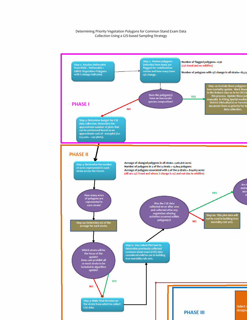
Determining Priority Vegetation Polygons for Common Stand Exam Data Collection Using a GIS-based Sampling Strategy
B-2
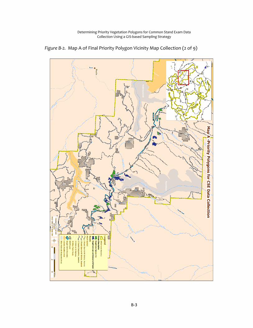
Determining Priority Vegetation Polygons for Common Stand Exam Data Collection Using a GIS-based Sampling Strategy
B-3
Figure B-2. Map A of Final Priority Polygon Vicinity Map Collection (2 of 9)

Determining Priority Vegetation Polygons for Common Stand Exam Data Collection Using a GIS-based Sampling Strategy
B-4
Figure B-3. Map B of Final Priority Polygon Vicinity Map Collection (3 of 9)
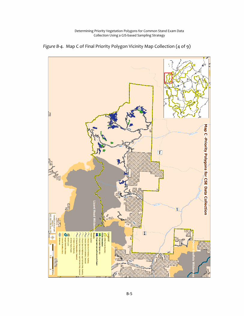
Determining Priority Vegetation Polygons for Common Stand Exam Data Collection Using a GIS-based Sampling Strategy
B-5
Figure B-4. Map C of Final Priority Polygon Vicinity Map Collection (4 of 9)
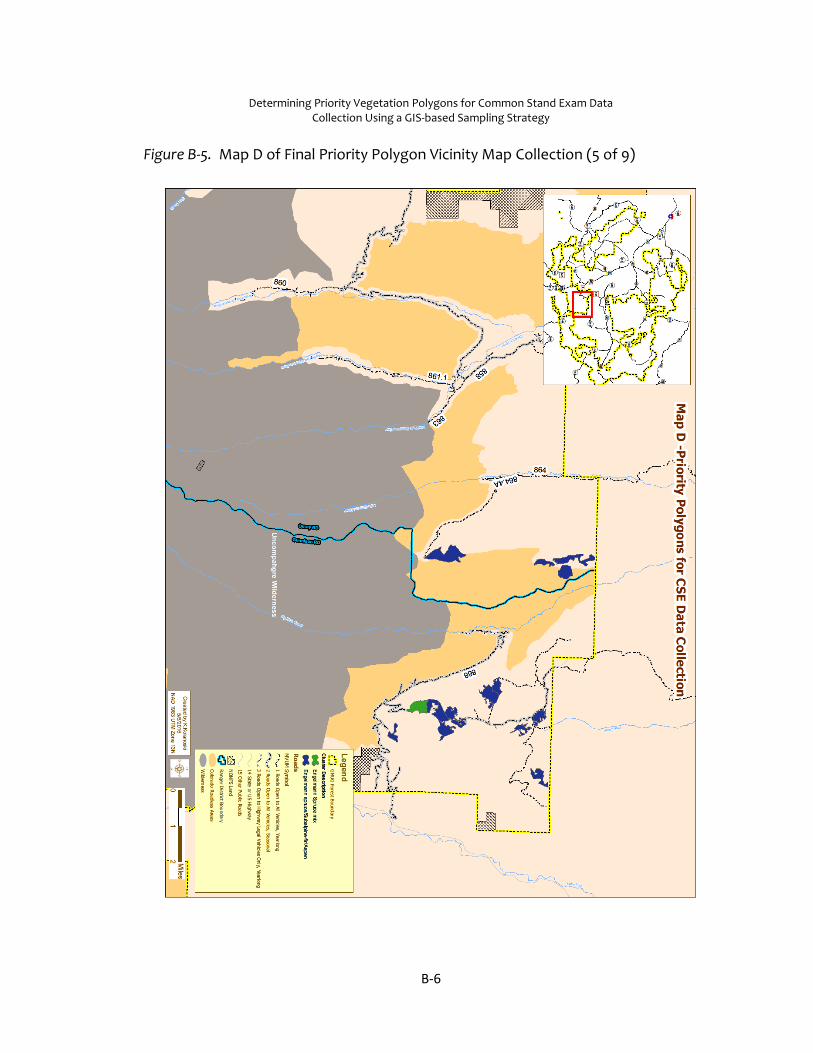
Determining Priority Vegetation Polygons for Common Stand Exam Data Collection Using a GIS-based Sampling Strategy
B-6
Figure B-5. Map D of Final Priority Polygon Vicinity Map Collection (5 of 9)
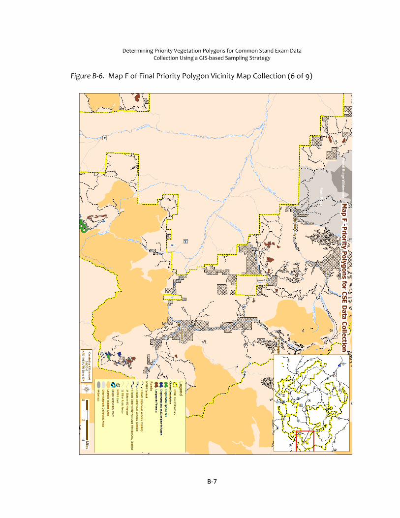
Determining Priority Vegetation Polygons for Common Stand Exam Data Collection Using a GIS-based Sampling Strategy
B-7
Figure B-6. Map F of Final Priority Polygon Vicinity Map Collection (6 of 9)
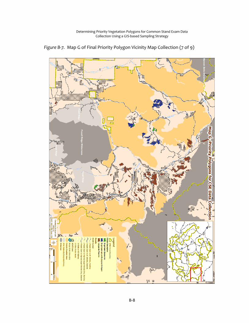
Determining Priority Vegetation Polygons for Common Stand Exam Data Collection Using a GIS-based Sampling Strategy
B-8
Figure B-7. Map G of Final Priority Polygon Vicinity Map Collection (7 of 9)

Determining Priority Vegetation Polygons for Common Stand Exam Data Collection Using a GIS-based Sampling Strategy
B-9
Figure B-8. Map H of Final Priority Polygon Vicinity Map Collection (8 of 9)
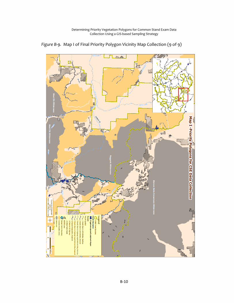
Determining Priority Vegetation Polygons for Common Stand Exam Data Collection Using a GIS-based Sampling Strategy
B-10
Figure B-9. Map I of Final Priority Polygon Vicinity Map Collection (9 of 9)