Embed Size (px)
Citation preview

Determining optimal discharge strategy for rechargeable lithium-ion batteries using multiphysics simulation
Leo L. Lam
A dissertation submitted in partial fulfillment of the requirements for the degree of
Doctor of Philosophy
University of Washington
2014
Reading Committee:
Robert B. Darling, Chair
Stuart Adler
Daniel Kirschen
Program Authorized to Offer Degree:
Electrical Engineering

© Copyright 2014
Leo Li Lam

University of Washington
Abstract
Determining optimal discharge strategy for lithium-ion batteries using multiphysics
simulation
Leo Li Lam
Chair of the Supervisory Committee:
Professor Robert B. Darling
Electrical Engineering
Lithium-ion rechargeable batteries have enabled the proliferation of mobile electronics
based on its high energy density, negligible memory effect and relatively high cycling capability.
Unfortunately, while small scale deployment in consumer-level electronics has been successful,
larger scale deployment for Electric Vehicles (EVs) or Hybrid Electric Vehicles (HEVs) have
been handicapped by the uncertainty of its long-term reliability, power density and safety.
Physical long-term testing requires months of waiting for the charge and discharge of the cells,
and while the electrochemistry models for the cells are well-documented, there is a lack of
modeling technique that bridges to the application level for electrical engineering designs.
This thesis addresses the modeling issue by presenting a novel method to use the detailed
electrochemistry-based model in real-world scenarios. The goal is to allow the simulations to be
sequentially run in different states based on the change in the physical parameters of the cells,
rather than switching between states using fixed time intervals. The method makes use of the

highly efficient partial differential equation solver in COMSOL to simulate digital, one-way
switching based on specific physical parameters.
The other issue this thesis addresses is the reduction of degradation in the long-term
cycling of lithium-ion batteries in larger-scale multi-cell applications. Using the detailed pseudo-
2D electrochemistry models, different discharge currents were simulated in a popular cell (Sony
18650) and the optimal current, and how this optimal current decreases as the cell cycles, is
presented. A 2-stage discharge method, used in conjunction with the penalty based switching
algorithm, was developed based on the modeling results of the low current degradation which
increases the per cycle discharge capacity by 5-10% while reducing the degradation on the anode
of the cell by approximately four times when compared to non-optimized discharge methods.
Overall, this research makes advances in the fields of sequential computer simulation of
physical systems and electrical engineering design for lithium ion battery systems in larger-scale
applications. The modeling method contributes to research opportunities in many fields, and the
determination of the optimal discharge current further enables the implementation of lithium-ion
batteries as the power source for EVs and HEVs.

i
Contents Chapter 1. Introduction and state of the art ..................................................................................... 1
1.1 Lithium-ion batteries ....................................................................................................... 2
1.1.1 History......................................................................................................................... 2
1.1.2 Operating principle of rechargeable lithium-ion batteries .......................................... 4
1.1.3 Performance advantages and limitations .................................................................... 7
1.1.4 Scale and economics ................................................................................................... 7
1.1.5 Performance metrics for lithium-ion cells .................................................................. 9
1.2 Degradation mechanisms .............................................................................................. 10
1.2.1 Overview ................................................................................................................... 10
1.2.2 Redox degradation at the electrodes ......................................................................... 14
1.2.3 Other mechanisms ..................................................................................................... 24
1.3 Degradation’s impacts on performance ........................................................................ 25
1.4 Contribution of this thesis ............................................................................................. 26
Chapter 2. Modeling the lithium ion battery ................................................................................. 28
2.1 Introduction and state-of-the-art ................................................................................... 28
2.1.1 Porous electrode theory ............................................................................................. 31
2.1.2 Pseudo-2D model ...................................................................................................... 35
2.1.3 Single particle model ................................................................................................ 40
2.1.4 Using COMSOL for simulation ................................................................................ 41
2.1.5 Limitations ................................................................................................................ 42
2.2 Low discharge current model development .................................................................. 43
2.3 COMSOL implementation ............................................................................................ 51
2.4 COMSOL implementation validation ........................................................................... 53
Chapter 3. Sequential simulation in COMSOL ............................................................................ 64
3.1 Development of sequential simulation method............................................................. 65
3.2 Implementation in COMSOL ....................................................................................... 69
3.2.1 Improvements since publication ............................................................................... 76

ii
3.3 Discussions, limitations and improvements .................................................................. 76
Chapter 4. Optimal discharge current strategy ............................................................................. 78
4.1 Introduction ................................................................................................................... 78
4.2 Multi-cell discharging schemes .................................................................................... 80
4.3 Trade-offs between different schemes .......................................................................... 82
4.3.1 Sequential discharge ................................................................................................. 82
4.3.2 Open-loop Switching (Sequential scheduling) ......................................................... 82
4.3.3 Close-loop Switching ................................................................................................ 83
4.4 Penalty based system .................................................................................................... 83
4.4.1 System description .................................................................................................... 84
4.4.2 Limitations in the theoretical penalty based model .................................................. 87
4.5 Determination of the optimal current (IOPT) .................................................................. 88
4.5.1 Analysis methodology .............................................................................................. 88
4.5.2 Results and discussions ............................................................................................. 90
4.6 Summary of observations ............................................................................................. 96
4.7 2-Stage discharge method ............................................................................................. 97
4.8 Application of the 2-Stage discharge method ............................................................. 101
4.8.1 18650 application test case ..................................................................................... 101
4.8.2 Test case results and discussions ............................................................................ 102
4.9 Implementation in real-world systems ........................................................................ 104
4.10 Conclusion .................................................................................................................. 106
Chapter 5. Conclusions ............................................................................................................... 108
5.1 Specific contributions ................................................................................................. 109
5.1.1 Sequential simulation in COMSOL ........................................................................ 109
5.1.2 Lithium ion battery low current degradation mechanism and expansion of existing
model 110
5.1.3 Optimal discharge current and strategy .................................................................. 111

iii
List of Figures
Figure 1. A common 18650 cylinder lithium ion rechargeable battery. Leo Lam © 2011. 2
Figure 2. Volumetric and specific mass energy density comparison between different
rechargeable battery chemistry [8]. ............................................................................. 3
Figure 3. Schematic diagram of the chemical reaction of a generalized lithium ion battery [8].
..................................................................................................................................... 5
Figure 4. Different capacity fade mechanisms at different state of charge . [3] ............... 13
Figure 5. Illustration to show the locations of the parameters for potentials and concentrations
before the values are abstracted. ............................................................................... 32
Figure 6. Macroscopic model as applied to the lithium ion battery structure using porous
electrode theory. ........................................................................................................ 33
Figure 7. Illustration of the lithium-ion flux at the boundary and within each abstracted sphere in
the solid matrix ......................................................................................................... 34
Figure 8. Illustration of the Newman pseudo-2D model. [83] .......................................... 35
Figure 9. The change of initial values of model parameters with cycles. ......................... 45
Figure 10. Illustration of a the Li-ion cell used in the pseudo-2D model. [5] [88] ........... 46
Figure 11. Geometry and coupling variables between the geometry of the P2D lithium-ion
battery model. The dotted arrows indicate the mapping of the boundaries. ............. 53
Figure 12. Comparing the output of the cell voltage (φ1) between the COMSOL model
implementation against Model 1. Solid lines represent the current model offset by 0.02 V
for clarity. Dotted lines were extracted from the reported data in Model 2. ............. 55
Figure 13. Comparing the concentration profile of the Li-ions in the electrolyte phase (c2)
between the COMSOL model implementation against Model 3. Solid lines represent the
current model offset by +2 mol/m3 for clarity. Dotted lines were extracted from the reported
data in Model 3. ........................................................................................................ 56
Figure 14. Potential profile of the Li-ions in the electrolyte phase (φ2) at different time. 58
Figure 15. Electrical potential profile of the Li-ions in the solid matrix phase (φ1) at different
times. ......................................................................................................................... 59
Figure 16. Electrolyte loss at different time in a sample discharge cycle at 0.5 C. .......... 60
iv
Figure 17. Overpotential for side-reaction in the anode in one full discharge cycle. ....... 61
Figure 18. Specific current density for the side reaction of electrolyte rate loss in the anode.
................................................................................................................................... 62
Figure 19. Concentration of lithium ions in electrolyte phase during discharge with a switching
event at 750 s. ........................................................................................................... 63
Figure 20. The lithium ion battery discharge/charge cycle, as a three-state, two-switch state
machine. .................................................................................................................... 64
Figure 21. Step function creating a 1-bit two-state change. ............................................. 65
Figure 22, The lithium ion battery discharge/charge cycle, as a three-state two-switch state
machine ..................................................................................................................... 66
Figure 23. Process flowchart for the sequential simulation calculation. .......................... 67
Figure 24. Illustration of the COMSOL smoothed Heaviside function flc1hs with a transition
time at t = 5 and different transition range. ............................................................... 68
Figure 25. The four-step differential equation based switching process .......................... 69
Figure 26. The simplified, two-state 1-bit switch, state machine. .................................... 70
Figure 27. Pulse generated by the subdomain expression for Switch............................... 71
Figure 28. Pulse integrated to become a non-reversible step function with adjusted conditions.
................................................................................................................................... 72
Figure 29. New IntSwitch value after implementing conditional applied current into boundary
condition. .................................................................................................................. 74
Figure 30. Discharge and charge current based on conditional switching. ...................... 75
Figure 31. Discharge-charge voltage curve based on conditional switching. ................... 76
Figure 32 Normalized discharge curves for an 18650 cell at different duty cycle. .......... 81
Figure 33. The penalty function per Adany et al. [98]. ..................................................... 86
Figure 34. Concentration loss plot against the normalized length of the cathode after Cycle 1.
................................................................................................................................... 91
Figure 35. Concentration of electrolyte loss at the cathode after one cycle at Cycle 1 at different
low discharge rate. .................................................................................................... 92
Figure 36. Concentration of electrolyte loss at the anode after one cycle at Cycle 1 at different
low discharge rate. .................................................................................................... 93

v
Figure 37. Electrolyte loss at 1 C discharge rate at three different discharge cycles. ...... 94
Figure 38. Variations of SOC at the 90%-loss level at the cathode and anode with cycle number.
................................................................................................................................... 95
Figure 39. Percentage of discharge time elapsed to reach 90% of maximum electrolyte loss per
cycle. ......................................................................................................................... 96
Figure 40. Discharge current profile for an 18650 cell with a switching time at 572s. .... 98
Figure 41. State-of-charge decreases in the anode at two different rate based on the 2-Stage
discharge method. The switching time depends on the state-of-charge corresponding to the
time at which the anode low current degradation tapers toward zero. ...................... 99
Figure 42. Modified Penalty curve for the discharge current in Stage 2. ....................... 100
Figure 43. Cycle 1. Relative change in discharge capacity and degradation of the 2-stage
discharge method in comparison with two CC type discharge. .............................. 103
Figure 44. Cycle 100. Relative change in discharge capacity and degradation of the 2-stage
discharge method in comparison with two CC type discharge. .............................. 103
Figure 45. Cycle 300. Relative change in discharge capacity and degradation of the 2-stage
discharge method in comparison with two CC type discharge. .............................. 104
Figure 46. Data flow in the control system based on the penalty-based algorithm. ....... 105
Figure 47. Data flow in the battery control system including the lookup table with data based on
modeled values. ....................................................................................................... 106

vi
List of Tables
Table 1. Notation and terms summary for the penalty-based algorithm ........................... 84
Table 2. Cycling parameters used in the study. ................................................................ 46
Table 3. Parameters for the cathode and anode materials. ................................................ 89

vii
ACKNOWLEDGEMENTS
This dissertation would not have happened without the tremendous amount of guidance,
support and perseverance from my long suffering Advisor Prof. R. Bruce Darling. He has
supported me throughout all of my endeavors, be it in research, teaching or business. He always
has my best interest in mind and has provided me with a great deal of freedom to explore
different possibilities, while keeping me on track as graduation time approached. Led by
example, he has inspired me to be rigorous in my work and meticulous in its execution. In short,
he has inspired me to be a better scientist, and a better person.
I would also like to thank Prof. Stu Adler for his guidance on the modeling aspect of this
work. Without the many conversations, especially in the beginning of the research, it would have
taken me much longer to understand the abstraction and terminology in the electrochemistry
world. His input on the revision of this dissertation was extremely valuable and has helped make
this study more complete. I am also indebted to him for the experience at the business plan
competition in 2007, when the team made an award-winning attempt to commercialize one of his
fuel-cell related patents.
To my other Committee members, Prof. Brian Fabien, Prof. Daniel Kirschen and Prof.
Guozhong Cao, thank you for taking the time to be on my committee. Thank you also for
providing me with concrete feedback on the revision of this dissertation and the support you
have shown me.

viii
Dr. Liney Arnadottir and Dr. Courtney Kreller, thank you for all the assistance in
electrochemistry modeling and COMSOL tips.
I would also like to thank Prof. Tai-Chang Chen, who proofread the first revision of this
dissertation and assisted me in the preparation of the Defense. His unwavering encouragement
and friendship throughout the past years have kept me focused and hopeful even during the most
difficult time. His belief in my ability was instrumental in the completion of this dissertation.
Prof. Jim Peckol, whose continued support has helped me through the most difficult
times. His wisdom, encouragement and support helped push me past the finish line.
Prof. Karl Bohringer, who sat on my General Exam committee and has provided me with
much support over the years. Thank you for believing in my ability and keeping me on track with
constant gentle nudging. Thank you also for the chance to teach the MEMS class with you.
I would like to particularly thank Frankye Jones, Erin Olnon and Brenda Larson at the
Advising Office, all of whom never doubted that this dissertation would be accomplished even
when I did. Thank you also for believing in my teaching work and continued to assign me classes
to teach over the past 6+ years.
To my fellow (former) graduate students and office mates, Dr. Hawkeye King, Dr. Sara
Rolfe, Tom Christiansen, Byron Wong, Dr. Shiho Iwanaga, Dr. Rachel Yotter, Dr, Hassan
Arbab, Dennis Meng and many more whom I have neglected to add to the list, thank you for
your support throughout the years and your never ending belief in me.
I would also like to thank all of my students, whom have placed your trust in me to help
you through your classes, and thank you for giving me the best education on humility and
empathy. It was an honor to have been your teacher.

ix
Thank you, Hannah Larson, for the love you have shown me and the unending care. This
would not have happened without you.
I would also like to thank many of my friends who have supported me over the years:
Guillaume Wiatr, Erin Skipley, Grace Gyurkey, Nirupama Kumar, Heather Boyko and family,
Gabe Brown, Taylor Corson, Mckenzie Such, Prof. John Castle, Prof. Alan Leong, Bill Lynes,
Brandee Slosar, Chris Maier, Olivia Lazer, Derek Merdinyan, Amber Favre, Leah Santa Cruz,
Lauren Witt, Erin Tinsley, Sarah Mcquaide, Sofia Kenny, Dr. Fred Holt, Richard Goldstein,
Stephen Graham, Valerie Trask, Lukas Svec, Pam Eisenheim, Helene Obradovich, Stephen
Graham, Lee Damon, Marek Mezyk and many more.
It truly took a village. Thank you.

x
DEDICATION
For my parents: Prof. Chiu-Ying Lam and Dr. Man-wan So who have taught me to be curious
and rigorous in the search of knowledge.
For my brother: Dr. Fung Lam, who has shown me that taking a path less traveled and then
achieving tremendous success is possible.

1
Chapter 1. Introduction and state of the art
Lithium ion rechargeable batteries have become the preferred choice of power sources for
consumer electronics and many other applications such as renewable energy storage. There is a
push for the next generation of electric vehicles (EVs) to transition the power sources toward
lithium ion batteries for the high energy density in volume and weight, lack of memory effect,
low self-discharge and high cyclability. Drive range and cycle life are the major factors that
determine the performance of the EVs [1]. Range is directly related to the discharge capacity of
the battery cell packs and cycle life is reduced by the internal degradation of the cell pack from
side reactions during the charge and discharge cycle. The other challenge for widespread
adoption involves the perceived safety hazard of the lithium-ion rechargeable cells.
Given the high cost of replacement [2], the amount of degradation due to cycling in real-
world usage situations must be minimized. Many degradation mechanisms have been suggested
and verified for both the charge and discharge cycle [3] and a selected subset of these
mechanisms in the charge cycle have been modeled based on first principles [4]. A semi-
empirical model to predict the capacity fade of the most popular Sony 18650 cell was reported
by Ramadass et al [5]. Discharge capacity fade was widely reported at high currents and was
simulated assuming a solution phase diffusion limitation and a different reaction rate distribution
[6].
In this introduction, a brief history of the lithium ion battery is discussed, including the
basic working principles and the performance metrics. A quick review of the state of the art in
the modeling of lithium ion secondary battery cells based on electrochemistry will follow, and
the pros and cons of each type of modeling are discussed. The electrochemical degradation
mechanisms that impact the performance of the cells are quantified.

2
The last sub-section summarizes the contribution of this thesis to the expansion of
knowledge in both the field of simulation and lithium ion battery application optimization.
1.1 Lithium-ion batteries
1.1.1 History
G. N. Lewis invented the first lithium-based
primary battery in 1912, and since that time engineers
began research to turn this into a secondary cell. Given the
reactive characteristics of lithium metal, many difficulties
had to be overcome, most importantly stability and safety.
A secondary battery based on lithium metal as the anode
and titanium (IV) sulfide as cathode was first reported by
Whittingham [7] in 1976.
The two major parts that needed attention were the
electrodes and the electrolyte. It took almost eighty years
of development for the first rechargeable lithium-ion battery
to be used on a mass-market level.
Sanyo made the first widely available commercial
version in 1991. Today, lithium ion batteries power all kinds of consumer electronics, from cell
phones to portable notebook computers and automobiles. This has been the result of extending
lithium metal chemistry to primary and secondary cells. By eliminating lithium metal from the
cells, the reaction is now safe and reversible over hundreds of cycles. Although the cost of
materials for manufacturing lithium ion batteries remain higher than that of its competing
chemistries, Nickel Metal Hydride (NiMH) or Nickel Cadmium (NiCd), due to recovery of
Figure 1. A common
18650 cylinder lithium ion
rechargeable battery. Leo
Lam © 2011.
3
development cost and the relatively low volume of lithium ion battery production, the chemistry
promises significantly lower cost per Watt-hr (Wh) in the future as production volume goes up.
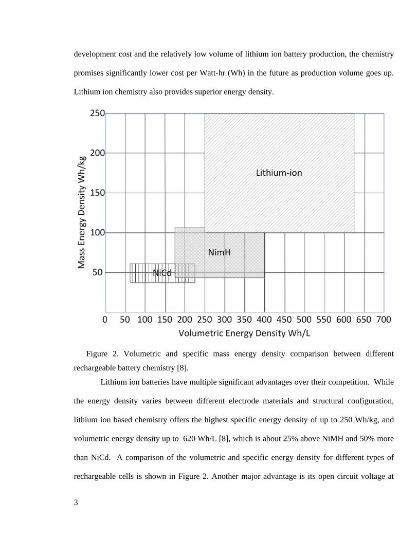
Lithium ion chemistry also provides superior energy density.
Figure 2. Volumetric and specific mass energy density comparison between different
rechargeable battery chemistry [8].
Lithium ion batteries have multiple significant advantages over their competition. While
the energy density varies between different electrode materials and structural configuration,
lithium ion based chemistry offers the highest specific energy density of up to 250 Wh/kg, and
volumetric energy density up to 620 Wh/L [8], which is about 25% above NiMH and 50% more
than NiCd. A comparison of the volumetric and specific energy density for different types of
rechargeable cells is shown in Figure 2. Another major advantage is its open circuit voltage at

4
around 3.7 V versus 1.2 V for the other two. It can provide high drain current of up to 3C (3
times the rated “Capacity” current) and exhibits virtually no memory effect. It has a very low
self-discharge rate and a high cycle-life at over 1,000 cycles to 80% of initial capacity. Due to
its specific charging curve, lithium ion batteries can be charged to 80% within one hour and be
fully charged in about 2 hours. Besides, lithium ion batteries are the most environmental-
friendly secondary cells on the market, containing no toxic “heavy” metals like cadmium, lead or
mercury.
In the following sections, the structure and the operating principles of the lithium-ion
battery will be presented, followed by a state-of-the-art review of its technical advantages and
limitations. The market size of the lithium ion secondary battery will be briefly analyzed and the
impact of improving the performance will be discussed.
1.1.2 Operating principle of rechargeable lithium-ion batteries
Rechargeable lithium ion batteries are structurally similar to other battery types,
consisting of a cathode, an anode and an electrolyte. Lithium ions move from the anode to the
cathode during discharge and vice versa during charge. The ions repeatedly intercalate and de-
intercalate between the two electrodes during cycling. This is unlike the single-use lithium
battery, which uses a metallic lithium film as its anode. This transfer of ions between the
electrodes is called the “rocking chair” or “swing” principle [9].

5
Figure 3. Schematic diagram of the chemical reaction of a generalized lithium ion battery [8].
The major difference in operating principle between lithium ion batteries and other
rechargeable battery types is that the electronic current is carried within the cell by a single ion
species, lithium ions, instead of multiple species, while electrons flow through the external
circuit to do work as shown in Figure 3. This necessitates the need for the electrode materials to
be both a good electronic conductor and a good ionic conductor.
Unfortunately, many electrochemically active materials are not good electronic
conductors, and carbon black is often used as a binder to such material. Most electrodes used in
modern rechargeable lithium ion batteries are complex porous composite materials.
The anode is generally made out of graphite or Mesocarbon MicroBeads (MCMB)
graphite powder, and it acts as the source of lithium. Carbon nanotubes have been reported to
significantly increase the energy density and reversibility for li-ion batteries [10] due to the
unique structural, mechanical and electrical properties. Using aligned carbon nanotubes, capacity
6
of 200 mAhg-1 and power density of up to 100 kWkg-1 have been reported by Lee et al. [11], and
silicon infused Si/C and Si/ composite nanofibers have been reported to yield a high current
density of 300 mAg-1. While these results are multiple times higher than the current generation of
commercial lithium-ion batteries, silicon structural damage and other manufacturing related
problems, have not yet allowed these materials to make it to commercialization.
The electrolyte is generally a lithium salt, like LiPF6, LiAsF6, LiClO4 and LiBF4,
dissolved in a mixture of organic solvents, like ethylene carbonate (EC) or dimethyl carbonate
(DMC). Some other electrolytes can be used in specialized applications such as those requiring
high temperature stability at the expense of lower conductivity and power density, but these are
beyond the scope of this thesis.
This liquid electrolyte acts as a carrier between the positive and negative electrodes when
current flows through an external circuit. Typical conductivities of liquid electrolyte at room
temperature (20 °C (68 °F)) are in the range of 10 mScm-1 (1 Sm-1), increasing by approximately
30–40% at 40 °C (104 °F) and decreasing slightly at 0 °C (32 °F).
Organic solvents easily decompose on the negative electrodes during charge. However,
when appropriate organic solvents are used as the electrolyte, the solvent decomposes on initial
charging and forms a solid layer called the solid electrolyte interphase (SEI), which is
electrically insulating yet provides significant ionic conductivity. The interphase prevents
decomposition of the electrolyte after the second charge. For example, ethylene carbonate is
decomposed at a relatively high voltage, 0.7 V vs. lithium, and forms a dense and stable
interface.
The most researched and commercialized type of cathode materials are layered
compounds with an anion close-packed lattice where a redox-active transition metal is located in

7
between these layers. Some examples include LiCoO2, LiMnO2, LiNi1-yCoyO2 and LiNiyMnyCo1-
2yO2 (NMC). LiCoO2 has been the cathode material of choice due to its high energy density but
has so far been limited to consumer electronics use due to safety issues, especially when it is
damaged. The other cathode materials, while offering slightly lower energy density, are safe
even when punctured. NMC, in particular, has been the material of choice for vehicular
applications.
Pure lithium is highly reactive. It reacts vigorously with water to form lithium hydroxide
and hydrogen gas, which can ignite. Thus, a non-aqueous electrolyte is typically used, and a
sealed container rigidly excludes moisture from the battery pack.
Lithium ion batteries are more expensive than NiCd batteries but operate over a wider
temperature range with higher energy densities. Due to flammable conditions that overcharging
could create, these cells require a protective circuit-based controller to limit peak voltage and
specific chargers.
For notebooks or laptops, lithium-ion cells are supplied as part of a battery pack with
temperature sensors, a voltage converter/regulator circuit, voltage taps, a battery charge state
monitor and the main connector. These components monitor the state of charge and current in
and out of each cell, the capacities of each individual cell (drastic change can lead to reverse
polarities which is dangerous), the temperature of each cell and minimize the risk of short
circuits.
1.1.3 Performance advantages and limitations
1.1.4 Scale and economics
The market for lithium ion batteries is experiencing significant changes across consumer,
automotive and industrial segments. One of the major contributing factors is the price reduction

8
of lithium-ion batteries due to industry over-capacity and competition. The proliferation of new
consumer gadgets and rapid strides taken by the battery industry to keep up will also give a
strong boost to the market. Electric vehicles, which have been on the cusp of strong growth for a
while now, are expected to help triple the automotive lithium-ion batteries market. The industrial
lithium-ion batteries segment too will grow on the back of stationary energy storage applications.
New analysis finds that the market earned approximately US$2.21 billion in 2012 and
estimates this to more than double to US$4.82 billion by 2017 due to the widening market and
product scope.
New energy storage applications in electric vehicles, grid-connected stationary energy
storage, and the higher energy requirements of new consumer products are expected to alter
market dynamics. The lithium-ion battery market has to make the most of these changes and find
usage in these application areas.
Lithium-ion batteries are the preferred energy sources for consumer products such as
phones, tablets, mp3 players, next-generation electrically propelled light motor vehicles, and
many industrial and commercial applications. In emerging consumer applications such as smart
phones and tablets, lithium-ion batteries are likely to generate high volumes but require
technology upgrades to grow faster.
Consumer products like smart phones and ultrabooks are energy intensive; however
battery technology has not kept pace with their growth. This has led to R&D for newer
chemistries in industrial and automotive segments that might prove disruptive to the lithium-ion
battery market.
With expectations of strong market growth, the competitive intensity and the production
capacity in the industry has dramatically increased. So, apart from infusing funds into R&D to

9
improve battery performance, manufacturers are resorting to price cuts to stay competitive. They
are also trying to increase product compatibility and decrease product prices to suit a wider
gamut of applications.
1.1.5 Performance metrics for lithium-ion cells
The measures of performance of lithium ion secondary batteries are the same as other
secondary batteries, namely discharge capacity and cycling life.
Discharge capacity can be measured by energy capacity (in Wh) relative to other
secondary batteries of different chemistry, or by charge capacity (in Ah) relative to cells of the
same chemistry. For lithium ion secondary batteries, this is generally measured by a low constant
current (C/2 or lower) discharge from its fully charged state to when the terminal voltage drops
to a specific end of discharge voltage (EODV), commonly in the 2.7-3.0 V range. The discharge
capacity is the product of the current and the time elapsed.
Based on the methodology, the measurements are affected by two factors: the true
capacity of the cell, and the internal resistance which causes the terminal voltage to drop as
current flows. The equivalent internal resistance of a lithium ion cell is increased by both
degradation products and the concentration gradient of the lithium ions formed within the cell.
Degradation mechanisms will be covered in the next section.
Cycling life is a measure of a secondary battery’s ability to go through charge and
discharge cycles. There is no specific standard on how the cycle life is measured. However, the
battery is commonly considered to be at the end of its cycle life when its discharge capacity has
dropped to 50% or 80% of its rated/new capacity. These criteria must be stated by the
manufacturers for comparison.
10
Cycling life is affected by many factors. Degradation causing side reactions physically
affect the electrodes, reducing their active surface areas and porosity. Film formation can both
prevent the lithium ions from intercalating into an electrode and increase the internal resistance
of the cell, leading to a superficial drop in discharge capacity.
1.2 Degradation mechanisms
1.2.1 Overview
Besides the intercalation and de-intercalation of lithium ions during charge and discharge,
side reactions and various degradation processes proceed concurrently. These processes
contribute to multiple undesirable effects, including gas accumulation, resistive film formation,
loss of active materials, loss of electrolyte, loss of active reaction surfaces and shorts. While this
study focuses on the capacity fade and its corresponding side reactions, it should be noted that
some of the processes can lead to fire and explosion via creating shorts and high in-situ pressure.
Both graphite and LiCoO2 are layered compounds that intercalate reversibly with lithium
in processes which are mainly phase transitions between stages of different degrees of lithiation.
While LiCoO2 electrodes insert lithium reversibly in any polar aprotic Li salt solution of
sufficient anodic stability, the process of Li insertion of graphitic carbon, as well as the stability
of graphite electrodes in Li salt solutions, is highly dependent on the composition of the
electrolyte solution. Hence, in both cases of Li metal-based and Li-ion rechargeable batteries,
their successful operation depends primarily on the performance, stability and reversibility of the
anode side (i.e., Li metal or graphite electrodes, respectively). Both Li metal and graphite
electrodes in a large variety of non-aqueous Li salt solutions have an important common
feature—in the same solutions, they are covered by very similar surface films, which in fact
control their electrochemical behavior. Lithium reacts spontaneously with all atmospheric gases

11
except noble gases, all polar aprotic solvents, and most of the commonly used salt anions (e.g.,
ClO4, AsF6, PF6, BF4, CH3CO3, and (CH3-SO2)2N ) to form Li salts, most of which are usually
insoluble in the other precursor solution [6]. These film formation processes passivate the active
metal and protect it from corrosion when the surface films become sufficiently thick to block
electron transfer. Due to the special properties of the lithium ion (e.g., its small size) and the
nature of its ionic bonds with other atoms, most of the Li salts precipitated as thin films conduct
electricity under an electric field. This is due to the fact that Li-ions are mobile in thin films of Li
salts and can thus easily migrate. This is known as the solid electrolyte interphase (SEI) model
for Li electrodes. It is generally known that Li deposition in many electrolyte solutions is highly
dendritic, and this makes these systems (electrode-solutions) unsuitable for secondary batteries.
Another highly important aspect regarding practical batteries is that of safety issues. As
already explained in detail, many lithium solution systems undergo a thermal runaway. Hence,
poorly designed rechargeable Li batteries can explode easily under abuse conditions such as
short circuit and overcharge, when they are punctured or crushed or when they are exposed to
high temperatures.
In recent years, rechargeable batteries with internal safety mechanisms have been
developed that prevent explosion of the batteries in the event of short circuit, overcharge, and
heating up to 150 degrees Celsius.
Over the past 15 years, the behavior of Li electrodes in a large variety of solutions have
been explored, using a variety of in situ methods, including Fourier Transform Infrared (FTIR)
spectroscopy, atomic force spectroscopy (AFM) and electrochemical impedance spectroscopy
(EIS). Researchers explored commercially available rechargeable Li–LixMnO2 batteries. These
studies included a rigorous postmortem analysis of cycled batteries. These studies have provided

12
a broad view of the intrinsic limitation of rechargeable Li battery systems with liquid electrolyte
solutions, and of possible useful future directions for R&D of practical rechargeable Li battery
systems. Similar to lithium, graphite electrodes polarized to low potentials in non-aqueous
solutions, containing Li salts, reduce the solution species to insoluble salts, and hence, become
covered by surface films of a chemical structure, similar to that of surface films formed on
lithium in the same solutions. For lithiated graphite, the major failure mechanism is
cointercalation of solvent molecules that are pushed together with Li-ions between the graphene
planes. In the absence of passivation, cointercalation of solvent molecules together with Li-ions
simply exfoliates the graphite and decomposes it to a dust of graphene sheets. Hence, a key
factor that determines the stability of graphite electrodes in Li insertion processes is to what
extent protective surface films are formed rapidly enough before cointercalation can take place.
During the past 10 years, the behavior of graphite electrodes in a large variety of electrolyte
solutions has been studied. Recently, these studies have also included postmortem analysis of
practical Li-ion batteries.
A summary of the side reactions and degradation processes is shown in Figure 4. This
study focuses on the processes that directly impact the capacity fade and life cycle reduction of
the lithium ion batteries, and in the following sub-sections, the relevant degradation processes
are discussed in detail.

13
Figure 4. Different capacity fade mechanisms at different state of charge . [3]
In this thesis, the assumption has been made that all of the lithium ion batteries being
considered are controlled by a competent battery management controller, such that overcharging
and over-discharging would not occur. The motivation of this part of the work is to investigate
the effect of an externally applied stimulus (applied terminal voltage) on the electrochemistry
behavior within the cell. It is desired that this investigation would ultimately lead to better energy
conservation through more efficient energy use. Manufacturer’s cell conditioning, cell balancing
and initial film formations are not controlled by users post deployments, and are considered out
of the scope of this thesis.
Cathode Anode
Oxygen evolution Li(s) deposition
Solvent oxidation Solvent reduction
Self discharge Self discharge
Transition metal dissolution
Jahn Teller Distortion Current collector dissolution
Charged
Discharged

14
1.2.2 Redox degradation at the electrodes
1.2.2.1 Electrolyte oxidation at the cathode
The cathode is the determining factor in the energy density, rate/power capacity and cost
of Li-ion batteries. Intensive research work on cathode materials has been carried out by many
research groups around the world. Materials currently being explored include LiMn2O4 spinel
[12], LiFePO4 [13] [14] [15], LiMn1-x-yNixCoyO2 [16] [17] [18], LiMn0.5Ni0.5O2 [19] [20] [21],
LiMn1.5O4 spinel [22] [23] [24], LiNi1-xMO2 (where M denotes a third metal like Al or Co) [25]
[26], LixVOy [27], and LixMyVOz (where M is a third metal such as Ca or Cu) [28].
These studies involve the development of reliable methods to produce these materials,
their structural analysis and electrochemical behaviors. Using the latest analytical tools like
synchrotron, X-ray radiation for in situ X-Ray Diffraction (XRD) [29], X-ray Absorption Near
Edge Structure Spectroscopy (XANES) [30], Extended X-ray Absorption Fine Structure
Spectroscopy (EXAFS) [31], high resolution scanning electron microscopy (SEM), electron
diffraction [32] and solid-state Nuclear Magnetic Resonance spectroscopy (NMR) [33], the
structural analyses are highly precise.
These electrode materials are reactive to the electrolytes forming very thin films to form
Solid Electrolyte Interphase (SEI) electrodes [34]. Surface analysis on these materials is more
difficult to analyze because the thin surface film can be greatly influenced by trace contaminants
in the solution even at very low ppm levels. The major reactions that are relevant to this thesis
are summarized later in this section.
The common electrolytes used in lithium-ion batteries are mixtures of solvents, mostly
organic and lithium salts. The most used solvents today are mixtures of propylene carbonate

15
(PC), diethyl carbonate (DEC), and ethyl methyl carbonate (EMC). Popular salts are LiPF6,
LiBF4 and LiClO4 as mentioned earlier.
High voltage positive electrodes used in lithium-ion batteries require very high
electrolyte stability and purity [35]. There are only limited choices in the electrolyte selection
because the maximum voltage of the cell is restricted by the decomposition potential of the
electrolyte. Most of the aforementioned electrolyte decompose at > 4.5V forming insoluble
products [36] [37] that can block pores of the electrodes, reducing the porosity of the electrodes
thus reducing the discharge capacity and also leading to gas formation, potentially causing a
safety hazard.
The EC/DMC combination, used both by Sony and other manufacturers has a high
resistance to oxidation as reported by Tarascon [38]. It has also been reported that the
electrochemical oxidation potential of PC is enhanced by the presence of electrolyte salts [39].
Since this oxidation reaction is irreversible, no thermodynamic open-circuit potential
exists, and these side reactions are often described by Tafel equations which give a finite rate of
the side reaction at all voltages, and increasing exponentially with increasing voltage [40]. The
decomposition potentials of many electrolytes are quite unclear due to the ambiguity in the
reported values, and simulation has often been run with an assumed value, then modified to
match experimental data [40].
The general solvent oxidation process is as follows
solvent → oxidized products + ne-.
Solvent that has been oxidized is lost, which leads to an increase in the concentration of
the salts. This in turn decreases the electrolyte level which negatively affects the cell capacity. If
gaseous products are built up within the cell, physical damage can occur to the electrode and
16
severely reduce the cell capacity, besides also becoming a safety hazard. If solid products are
formed, these products can form a passivating film on the electrodes with higher resistivity,
which increases the polarization of the cell and lowers the output voltage of the cell. This causes
the discharge to reach the end of discharge voltage prematurely, effectively reducing the
discharge capacity of the cell.
The rate of solvent oxidation depends on the surface area of the cathode, current
collectors and the carbon black additive.
It has been reported that PC oxidizes at potentials as low as 2.1 V vs. Li/Li+ on a Pt
reference electrode [41], and the rate of oxidation increases substantially above 3.5 V, although
in practice PC is quite stable even at 4.5 V. Similar results were observed by Cattaneo et al. [42]
and Eggert et al. with LiClO4 salt in PC [43].
Decomposition of the ClO4- ions above 4.5 V vs. Li/Li+ forms chlorinated species ClO2
and HCl [42]. The reactions are as follows.
ClO4- + ClO4 + e- → ClO2 + 2 Oad + e-
ClO2 + H+ + e- → HCl + O2(g)
The instability of ClO2 combined with the protons from the oxidation of PC produces
HCl and oxygen evolution is also observed in the decomposition of LiClO4 electrolytes.
Christie et al. studied the oxidation potential of LiPF6 in PC with a Ni microelectrode
[44], and Kanamura et al. reported the PC oxidation potentials on Pt, Al, Au and Ni electrodes to
be from 4.5 V for Ni to 6 V for Cu vs. Li/Li+ [45] [46]. It was also observed that the anodic
behavior of Ni electrodes in different PC-based electrolytes depends on the type of electrolyte
salt used, and that the decomposition product depends on the type of anion in the high electrode
potential range.

17
More recent studies have shown that the intrinsic anodic stability of polar aprotic
electrolyte solutions for lithium ion batteries is mostly determined by the solvents and not the
salts used [47]. The common electrolytes can be classified into three categories.
1. Electrolytes with ether C-O-C type linkages, including both ethereal solutions and
polymer electrolytes based on polyethers or its derivatives. The oxidizing potential is low
at below 4 V vs. Li/Li+ [48] due to the limited anodic stability of the linkage. Given that
lithium ion batteries, when fully charged, run at over 4.2 V, these electrolytes are not
desirable.
2. Electrolytes with solvents such as organic esters or alkyl carbonates, and gel systems with
alkyl carbonates. These electrolytes have a good electrochemical window for oxidation at
over 4.5 V [49]. Some examples are polyvinylidene fluoride (PVDF) derivatives or poly
polyacrylonitrile derivatives mixed with Li salts and alkyl carbonate solvents.
3. Derivatives of imidazolium or pyrrolidinium salts have high anodic stability at over 5 V
vs. Li/Li+ [50]. This electrochemical properties is popular but the applicability for
practical use is still questionable [51].
Out of the three categories, the alkyl carbonate solvents, with very reasonable
performance at low temperature, are the most important for the voltage range of the Li-ion
batteries [52] and have been studied extensively. Using in situ FTIR spectroscopy and EQCM,
Moshkovich et al. found that the solvents can be oxidized on Pt at potential above 3.5 V vs.
Li/Li+, but the rate is very slow below 4.5 V [53]. It was also noted that the products formed
from the degradation processes under 4.5 V does not precipitate as a film, but as gaseous
products CO and CO2. Significant oxidation of the alkyl carbonate solvents occur over 4.5 V vs.
Li/Li+, and does affect the passivation film and processes.

18
1.2.2.2 Electrolyte reduction at the anode
Similar to electrolyte oxidation in the cathode, electrolyte reduction also causes capacity
fade and reduction of cycle life by consuming salt and solvent [38] [54] [55] [56]. This process
can also produce gaseous products, which can be a safety hazard.
Electrolyte reduction is an expected event of all carbon-based insertion electrodes due to
the instability of the electrodes to the carbon electrode under cathodic conditions. Ideally,
electrolyte reduction is confined to the formation period.
The decomposition mechanism was reported by Dey [57].
2Li++2e- + (PC/EC) → [propylene(g)/ethylene(g)] + Li2CO3
This reaction occurs during the first discharge when the potential of the electrode is near
0.8V vs Li/Li+ [58].
A similar reaction mechanism was proposed by Fong et al. for a mixed EC/PC electrolyte
[36].
While Dey et al. stated that the process is a two-electron process [57], Aurbach et al.
suggested that a one-electron intermediate step is involved [59] [60] [61]. They observed
ROCO2Li species and propylene in a one-electron reduction on graphite, and that ROCO2Li is
highly reactive to water to form Li2CO3.
They also stated that the carbon electrode could retain its graphitic physical structure and
undergo reversible intercalation in the presence of crown ethers because the solvent is not
intercalated and reduced on the surface but not within the carbon structure. When the reduction
reaction occurs on the surface, the charge transfer is accomplished mostly through existing films;
in this case, a one-electron process is favorable because the driving force of PC reduction is
reduced. If crown ethers are absent, the graphite/carbon electrodes were damaged [57]. In this

19
case, the PC molecules were reduced within the electrode, indicating cointercalation, and a two-
electron process to form Li2CO3 is more favorable.
Matsumara et al. observed an extra pathway for PC decomposition [62] during first
charge besides the direct 2-electron process mentioned above. This second pathway involves PC
undergoing reduction to form a radical anion, then a lithium alkyl carbonate by radical
termination. These intermediate products are unstable and react with propylene to form oligomer
radicals, and finally oxidize to compounds with C-H bonds and COOH groups. Shu et al., using a
1 M LiClO4 PC/EC (1:1) electrolyte, suggested another two-electron reduction process [63]. The
first process involves a two-electron reduction of PC and EC to propylene and ethylene gases
and the second is a one-electron reduction to form lithium alkyl carbonates. The two-electron
process can also be subdivided into an electrochemical component and a chemical reduction.
Both electrochemical reduction and SEI film formation paths involves the formation of lithium
carbonate complexes, which then goes through another single electron reduction to a radical
anion. This radical anion reduces further to yield gaseous products or terminal to form the SEI
film.
Material geometry also plays a role in the surface film formation degradation processes.
Using atomic force microscopy, Chu et al. studied the surface films formed on highly ordered
pyrolytic graphite (HOPG) electrodes during cathodic polarization in 1 M LiClO4 EC/DMC (1:1)
and 1 M LiPF6 EC/DMC (1:1) electrolytes [64]. It was observed that the irreversible side
reaction occur on edge surfaces at a higher potential than on the basal surface, at 1.6 and 2 V vs.
Li/Li+ and 0.8 and 1 V vs Li/Li+ respectively. Chu also discovered the thickness of the surface
film is a few hundred nanometers thick, much more than previously believed.

20
Further observation by Bartow et al. showed that solvent reduction is more dominant on
the basal surface while more salt reduction occurs on the edge surface [65].
SO2 has been shown to promote the reversible intercalation-deintercalation of lithium
ions into graphite in some nonaqueous electrolytes if added in large amount. SO2 forms fully
passive films on the graphite electrode at potentials much higher than that of the electrolyte
reduction. The reactions to form these films are as follows
SO2 + 6Li+ + 6e- → 2Li2O + Li2S
Li2O + 2SO2 → (LiO)2SO
A patented DEC and DMC based electrolyte [66], through ester exchange, forms methyl
ethyl carbonate [67]. This electrolyte has been reported to have desirable passivation properties,
with an effective reference voltage of 1.5 V vs. Li/Li+. Many carbonate-based solvents have also
reached the market, like chloroethylene carbonate (CEC), PC, EC mixture. [68] [69]. The
mixture forms a stable passivating film on the carbon electrode, and the small amount of
sacrificial carbonate is added to be consumed in the initial film formation cycle in order to
preserve the active solvent.
A summary of the major degradation mechanisms for the most used solvents, salts and
contaminants are given below.
Propylene carbonate (PC, solvent): 2-electron reduction process [57].
23PC + 2e- propylene + CO −→
The one-electron mechanism for PC reduction per Aurbach is
PC + 2e- → PC- radical anion
( ) ( ) ( )( ) ( )
- - -3 2 3 3 3
3 2 2 2
2PC- radical anion - propylene + CH3CH CO CH CO CH CH CO + 2Li
CH CH OCO Li CH OCO Li s
→ + −
→

21
– (Li alkyl carbonate)
Ethylene carbonate (EC, solvent): 2-electron reduction process, similar to PC.
23EC 2e ethylene CO −+ − → +
And the one-electron process is also similar to EC.
EC + 2e- → EC- radical anion
( ) ( ) ( )- - - +2 2 2 2 2
2 2 2 2
2EC- radical anion - ethylene + CH2 OCO CH OCO CH OCO + 2LiCH (OCO Li)CH OCO Li(s)
→
→
– (Li alkyl carbonate)
The lithium alkyl carbonate compound in both the PC and EC cases is a highly effective
passivating layer compared to Li2CO3.
Dimethyl carbonate (DMC, solvent) – single electron reduction
CH3OCO2CH3 + e- + Li+ → CH3OCO2Li + CH3*
or
CH3OCO2CH3 + e- + Li+ → CH3OLi + CH3OCO*
Both radicals formed are then converted to CH3CH2OCH3 and CH3CH2OCO2CH3 [70].
Diethyl carbonate (DEC, solvent): 2-electron reduction
CH3CH2OCO2CH2CH3 + 2e- + 2Li+ → CH3CH2OLi + CH3CH2OCO*
or
CH3CH2OCO2CH2CH3 + 2e- + 2Li+ → CH3CH2OCO2Li + CH3CH2*
The two radicals are then converted to CH3CH2OCH2CH3 and CH3CH2OCO2CH2CH3.
Salt reduction: The particular salt used affects the functioning of the carbon electrodes
because salt reduction also causes surface film formation. Depending on the species and solvent,
the surface film can be either passivating or it may interfere with the reduction products of the
22
solvent. The reduction reactions for the most used salts are summarized below. LiAsF6 and LiPF6
reduction occur at < 1.5 V vs. Li/Li+ [71].
LiAsF6 [60] [61]:
LiAsF6 + 2e- + 2Li+ → 3LiF + AsF3
AsF3 + 2xe- + 2xLi+ → LixAsF3-x + xLiF
LiClO4 [60]:
LiClO4 + 8e- + 8Li+ → 4Li2O + LiCl
or
LiClO4 + 4e- + 4Li+ → 2Li2O + LiClO2
or
LiClO4 + 2e- + 2Li+ → Li2O + LiClO3
LiPF6 [61] [70]:
LiPF6 ⇄ LiF + PF5
PF5 + H2O → 2HF + PF3O
PF5 + 2xe- + 2xLi+ → xLiF + LixPF3-x
PF3O + 2xe- + 2xLi+ → xLiF + LixPF3-xO
and
6 3PF 2e 3Li 3LiF PF− − ++ + → +
LiBF4 [61]: Similar to LiPF6.
4 4BF e 2 Li Li BFxx x xLiF− − ++ + → +
Contaminant reduction:
Small traces of oxygen and water contaminants in the electrolyte can be reduced to form
lithium oxide [60].

23
- +2 2
1 O +2e +2Li Li O(s)2
→
Though very rare in the latest lithium ion battery cells, water with concentration higher
than 300 ppm can lead to the formation of LiOH, which coats the surface of the carbon with a
high resistance film. This film can completely prevent lithium ions from intercalating into the
electrode. The reaction is
- -2 2
1H O+e OH + H2
→ ↑
+ LiOH(s)Li OH →+ −
- +2 2
1LiOH(s)+e +Li Li O(s) H2
→
Carbonate can also formed through reduction of CO2 if a high enough concentration is
present.
- -2 2 32CO +2e +2Li Li CO +CO→
or
- - - +2 2CO +e +Li CO Li→ ⋅
- +2 2 2CO Li +CO OCOCO Li⋅ →
- +2 2 3OCOCO Li+e +Li CO+Li CO→
Lithium carbonate can also be formed via secondary reactions. This reaction occurs at
potentials less than 1.5 V vs. Li/Li+) [60].
2 2 2 2 3ROCO Li+ O 2ROH+CO +Li COH →
where R is an ethyl or propyl group.

24
1.2.3 Other mechanisms
1.2.3.1 Cathode dissolution
LiCoO2 electrodes generally cycle well even at temperature above 60 oC if the solvent is
salt-free [72]. However, if a salt, like LiPF6 is present, dissolution of the Co occurs under two
different circumstances.
1. Presence of LiPF6 causes Co dissolution. This is exacerbated with water contaminants.
Higher temperature also increases the rate of dissolution.
2. A composite LiCoO2 electrode with a PVDF binder incurs the highest rate of Co
dissolution.
Particularly with LiPF6 which undergoes thermal decomposition to form traces of PF3O
and 2HF, it was also shown that LiCoO2 can catalyze the decomposition of the alkyl carbonates
to form gaseous product like CO2. Meanwhile, this process involves the reduction of Co3+ and
Co2+ ions; both are easily dissolvable in solutions. The reaction is
4LiCoO2 → CoO2 + CoIICo2IIIO4 + 2Li2O
then
Li2O + 2HF → 2LiF + H2O
where LiF is a highly resistive film [73]. This reaction is autocatalytic since H2O reacts
with LiPF6 to form more HF, which is needed for the reaction.
The major problem with cathode dissolution is that the presence of Co ions in the
solution invariably leads to the deposition of Co compounds (or metal) on the negative electrode.
Such precipitation is detrimental to the passivation of the Li-carbon anode and also hinders
repeated intercalation.

25
1.3 The impact of degradation on performance
The performance of a rechargeable battery is based on discharge capacity and cycle life,
as stated in section 1.1.5. In the last section, the set of degradation mechanisms have be
summarized and discussed, all of which are linked to the capacity fade in the short and long
terms.
Three factors directly affect the capacity fade: Loss of electrode material, loss of active
material (lithium ions) and prematurely reaching the end of discharge voltage (EODV).
Redox reactions on both electrodes result in the loss of electrode materials and the
consumption of Li-ions. The product of the dissolution of the cathode material coats the anode
with an electrically insulating film, plugging pores and lowers the available intercalation surface
area, directly reducing the cell capacity. This change in electrode porosity also affects the solid-
phase diffusion of Li-ions once intercalated [74].
Through the repeated intercalation and de-intercalation cycling of the cells, both
electrodes experience volume change. AFM studies have confirmed this [75]. While this volume
change is mostly reversible, drastic change in volume due to high discharge rate causes cracks to
form which opens up more highly reactive graphite electrode for the active species in the redox
degradation mechanisms to percolate through [76]. This, in turn, creates new sites for the
formation of the SEI film and for the more resistive products of the degradation reactions to
precipitate, increasing the internal resistance. This resistance causes an Ohmic drop in voltage at
the terminal as current passes, which leads to a prematurely reaching of the EODV.
These effects can be modeled through the addition of a film resistance, reducing the
initial state-of-charge [77] and gradually changing the diffusion coefficient term in the solid-
phase, which will be discussed in the next chapter.

26
1.4 Contribution of this thesis
This thesis explores and expands the use of the comprehensive pseudo-2D
electrochemistry based model of the insertion electrode Li-ion batteries by the addition of
degradation mechanisms at both electrodes during discharge. By considering the effects of such
degradation both spatially and in time, the study devises a predictive model that leads to an
optimal discharge strategy that can minimize the long-term degradation of such cells in
automotive applications. The work contributes specifically in the understanding of the
connection between terminal voltage based application level battery controller algorithm designs
to the fundamental physics of a single cell.
This work makes extensive use of the COMSOL Multiphysics package, and during the
evolution of the research, a new method to perform sequential simulation with changes of
boundary conditions based on the change of internal physical parameters was developed [78].
Prior to this work, the change in any boundary conditions could only be performed based on
time. This work significantly opens up the research capabilities of COMSOL. The method makes
use of the highly efficient partial differential equation solver in COMSOL to simulate digital,
one-way switching based on specific physical parameters.
Expanding on the current work on lithium-ion battery modeling, this study considers the
electrochemical side reactions occur during the discharge cycle, specifically at low level
discharge currents using the most rigorous pseudo-2D model. The new model allows for the
continuous calculation of the electrolyte loss and the subsequent forming of the highly resistive
film coating on both electrodes both spatially and in time. This provides the visualization of the
internal parameters, such as potentials and lithium ion concentration gradients, during discharge

27
throughout the cycle life of the cell beyond the terminal voltage, which is normally the only
measurable parameter once the cell is deployed. This allows for the prediction of the variation of
multiple degradation related variables and the examination of many internal cell parameters that
affect side reactions rates.
Based on the model developed and the results of the simulations, this thesis addresses the
reduction of degradation in the long-term cycling of lithium-ion batteries in larger-scale multi-
cell applications. Using the detailed pseudo-2D electrochemistry model, different discharge
currents were simulated using the parameters of a popular cell (Sony 18650) and this study
determines a discharge strategy that can improve the per cycle discharge capacity of the cell
without incurring penalizing degradation. This result directly applies to load balancing in large-
scale multi-cell battery system by current steering. All the degradation mechanisms known at the
time of writing were reviewed to determine the relevant processes that can be controlled and
measured from the terminals, discussed in detail in Section 2.2. Combining the new work and the
results derived from past work by others in the medium to high current discharging region, the 2-
stage optimal discharge strategy is presented in Chapter 4.
Overall, this research makes advances in the fields of sequential computer simulation of
physical systems, electrochemistry simulation of lithium ion batteries and electrical engineering
design for the application of lithium ion batteries in larger-scale applications. The COMSOL
switching method contributes to many research opportunities. The expansion of the existing
pseudo-2D electrochemistry model of the lithium ion battery creates a direct link between battery
management system design to the internal chemistry of the cells. The determination of the
optimal discharge current strategy further enables the implementation of lithium-ion batteries as
the power source for EVs and HEVs.

28
Chapter 2. Modeling the lithium ion battery
2.1 Introduction and state-of-the-art
The literature on modeling of lithium ion batteries is extensive [80] [81] [82]. The
rigorous physics-based modeling of Li-ion batteries that includes the internal electrochemistry of
the insertion electrodes was first proposed by Doyle, Fuller and Newman [83] [84] in 1993 under
limited cases and assumptions. Prior to that, the modeling of solid state battery systems with
insertion electrodes was limited to the use of dilute solution theory and porous electrode theory
[85]. The transport of electrolyte in the liquid phase was described by simple diffusion and
migration, the dilute solution theory, which was insufficient when ion pairing and ion association
are involved in the conduction in the electrolyte phase.
Doyle et al. proposed the use of concentrated solution theory, originally developed by
Newman [86], which provides a much more general and rigorous theoretical framework that
addresses the deficiency in the description of the transport mechanisms and accounts for volume
changes and electrolyte flow.
The development and extension of this model has been extensive. This full pseudo 2D
model based on porous electrodes and concentrated solution theory is used in this thesis to fully
study the behavior of the cell given the wide range of currents used, and the fact that the
simplified single-particle model is limited to the application of low cycling current. The limiting
electrode for cycle life is the negative graphitic carbon electrode. Thin film formation at the
porous carbon anode during the charging cycle causes potential drop in accordance with Ohm’s
Law. The lower conductivity by-product of this film also reduces the effective solid state
diffusion coefficient of the electrode. Ramadass et al. addressed these effects semi-empirically
by modifying three parameters, namely Rf (film resistance), State-of-Charge (SOC) loss and the
29
solid state diffusion coefficient based on first principles [5] and fitted to experimental results.
The SOC is defined as the ratio between the intercalated lithium concentration and the maximum
capacity concentration in the anode. Sikha et al. included the change in the porosity of the
electrode material over time [74]. In all of these models, the concentration of lithium within the
solid phase was calculated using superposition [87] or solved using a pseudo second dimension
(Pseudo-2D or P2D) along the radius of the particle based on diffusion. In most cases, since only
the concentration of lithium at the surface of the particle surface is of interest, limited computing
power makes the solving these models time consuming. This model is the choice of this thesis
and it will be discussed in detail in section 2.1.2. Further extension including thermal effects was
reported by Cai [88] et al. Capacity fade mechanisms under high discharge rates were analyzed
and characterized by Ning et al. through SEM and EIS studies [76], which further confirmed the
solvent decomposition mechanisms.
Wang et al. [89] and Subramanian et al. [90] presented a simplified model with very good
approximation of the concentration profile based on the integral approach by Ozisik [87]. The
concentration profile inside the solid particle is approximated by a second-degree polynomial
whose coefficients are expressed in terms of the average concentration of lithium inside the
particle and the concentration at the surface. This effectively eliminated the need to solve the
differential equation required for the concentration profile inside the particle. This is known as
the Polynomial Approximation model (PP).
Further simplification to the modeling of the electrode was presented by Haran et al. [91].
The simplified model used a single spherical particle to represent the whole electrode, while the
models described previously adopt the porous electrode theory approach. This method was
originally used for nickel metal hydride systems, and was adopted to the lithium ion system [92].
30
This model is known as the Single Particle model (SP). The SP model will be discussed in
further detail in section 2.1.3.
Each of the models described above has pros and cons compared to the others. The
porous electrode models have the advantage of showing a detailed account of almost the
complete set of physical processes inside the battery. However, with all the parameters being
simulated simultaneously, it is computationally complex and, therefore, time consuming.
The Single Particle model assumes a uniform concentration across the length of the
electrode, and that the solution phase diffusion limitations and concentration gradients are
ignored. Because of these simplifications, multiple variables are now abstracted as an average
throughout the electrode, and the model is more computationally efficient. However, the validity
of this model is therefore limited to pseudo steady state conditions, that is, very low current
galvanostatic charge and discharge such that the latter two assumptions remain true.
Using the polynomial approximation in the solid phase concentration calculation with the
P2D framework, the level of detail is mostly preserved and at the same time the simulation time
can be reduced. However, since this model focuses on solving for the surface concentration of
the particle, it is not flexible enough to account for the porosity change and diffusion coefficient
change due to degradation mechanisms.
In simulating the performance of a lithium ion battery’s cycle life, the battery model has
to be solved repeatedly over hundreds of cycles. This would demand that the model is not time
consuming, which makes the two simplified models attractive. A comparison in accuracy was
discussed by Santhanagopalan et al. [93]. It was reported that the both simplified models perform
well up to 1 C rate of discharge and that using the second order approximation significantly
reduced simulation time with good correlation to the rigorous P2D model. However, since the

31
solution phase limitations are ignored in the Single Particle model, it is unsuitable for higher
discharge current.
The Polynomial Approximation model (PP) was found to be suitable for higher discharge
rate above 1 C. The loss of accuracy was minimal but the computation time is greatly reduced.
2.1.1 Porous electrode theory
The porous electrode theory was formalized by Newman and Thomas-Alyea [86]. It
specifically addresses the type of materials used in the electrodes of lithium ion batteries. The
complete detail can be found in the corresponding chapter in the book referenced, and a
summary as it has been implemented in this study is given in this section.
A porous electrode is a porous reactive electronic conductor or mixtures of solids that
include both non-conducting, reactive materials and electronic conductors. Besides the solid
areas, the void is filled with electrolytic solution spaces between the solid matrix. Physically, the
reaction rates in a porous electrode can differ within the structure depending on the physical
structure, conductivity of the matrix and of the electrolyte, and also the parameters that
characterize the electrode processes.
Theoretical analysis to this complex issue requires a model that accounts for the essential
features of an actual electrode without going into exact geometric details. The model described
here was developed by Newman and Tiedemann [94] [95], which has been widely adopted and
refined by other researchers for lithium ion battery analysis.
The porous electrode theory was developed such that the parameters of the models can be
obtained by simple physical measurements and are geometry agnostic. These parameters include
porosity (void volume fraction), average surface area per unit volume and volume-average
resistivity. The model would use the averages of various variables over a region of the electrode
32
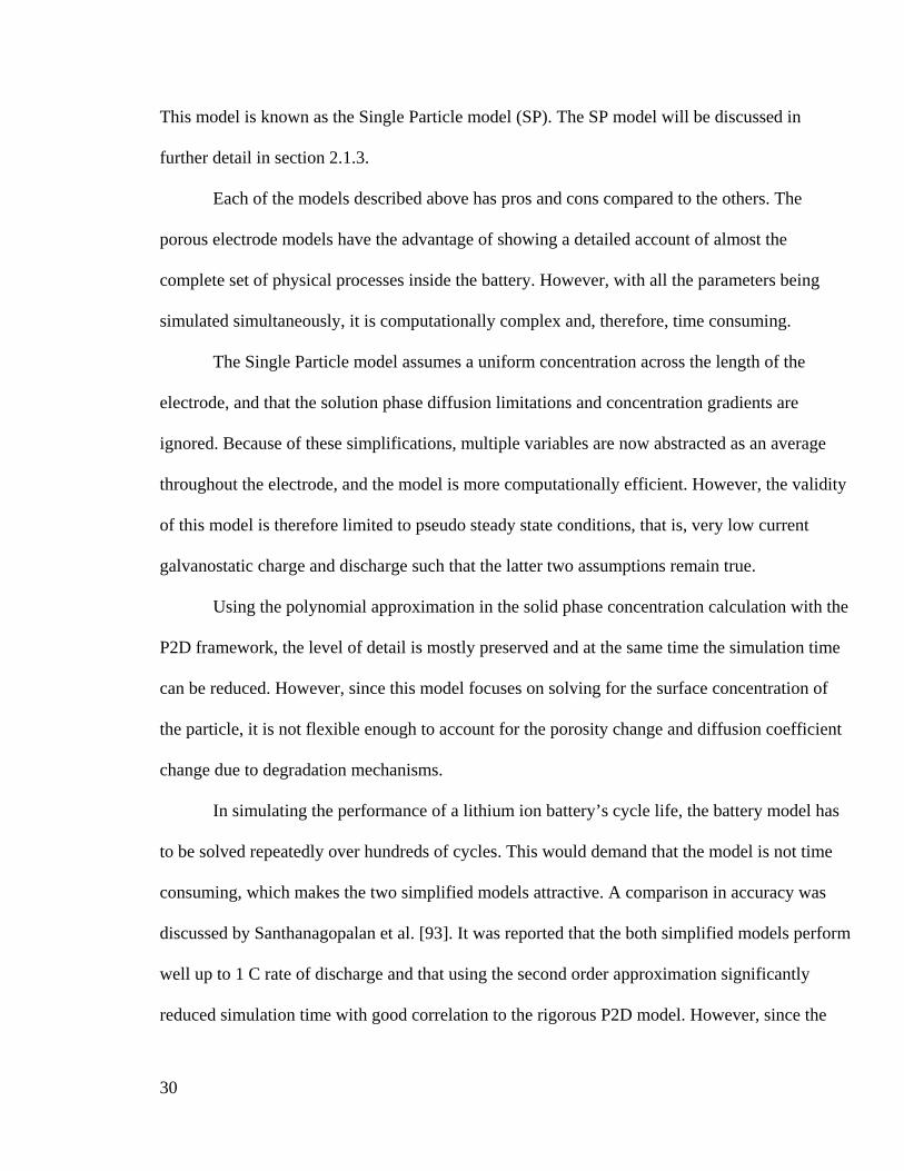
that is small with respect to the overall dimensions but large enough compared to the pore
structure. The rates of reactions and double-layer charging in the pores are defined in terms of
transferred current per unit volume. This is referred to as the macroscopic model. The parameters
that need to be abstracted are the concentrations of the lithium ions in the solid phase and the
electrolyte phase, and the potentials of the ions in each phase. The locations of each of these
parameters are shown in Figure 5.
Insertion electrode
C2
C1
φ2 φ1
Figure 5. Illustration to show the locations of the parameters for potentials and concentrations
before the values are abstracted.
With this treatment, two potentials can be defined, φ1 for the solid phase and φ2 for the
electrolyte/liquid phase. Both potentials are continuous functions of time and space coordinates.
The full electrode is then treated as the superposition of the two continua, one being the solution
and the other representing the solid matrix. The abstraction is illustrated in Figure 6.
The top axis represents the abstracted cell, with all three regions. In either electrode,
each point in x is mapped onto a spherical particle with radius R. The surface receives the flux
based on the interfacial reaction rate, and the flux is spread over its specific surface area ai,

33
which is is then defined as the surface area of the pore walls per unit volume of the electrode
scaled by the porosity εi and the volume fraction εf of the filler electrolyte.
2
, ,3
4 3(1 ) (1 )43
i i f i i f iRa
RRπ ε ε ε επ
= − − = − − (2.1.1)
As implemented in the lithium ion battery electrode, the porosity is the void volume
fraction ε within a volume element in the electrode that is filled with an electrolyte as shown in
Figure 5. The solution-phase concentration of the lithium ion is denoted c2 and this
representative concentration is averaged over the pores. c2 is also used to correlate the
composition dependence of the diffusion coefficients, activity coefficients and the conductivity
of the solution phase. This volume element also contains the solid matrix.
R
Separator Positive ElectrodeNegative Electrode
R R R
Figure 6. Macroscopic model as applied to the lithium ion battery structure using porous
electrode theory.
The average pore wall flux over this interfacial area a is the pore wall flux density Ji,
where i denotes the corresponding electrode, in this case, p or n. The average pore wall flux

34
density is the normal component of the flux density at the pore wall, in the direction pointing into
the solution. Combined, aJi is the rate of transfer of lithium ion from the solid phase to the
electrolyte/liquid phase. The relationships between the lithium ion flux on the surface and the
Figure 7. Illustration of the lithium-ion flux at the boundary and within each abstracted
sphere in the solid matrix
reaction rate, and the diffusion of the intercalated lithium ions within the sphere are shown in
Figure 7.
In order to model the material balance of the solutes, an average flux density Ni of the
species i over the cross-sectional area of the electrode is defined. For this plane surface, Ni
represents the amount of species crossing the plane in the electrolyte phase. Hence, assuming a
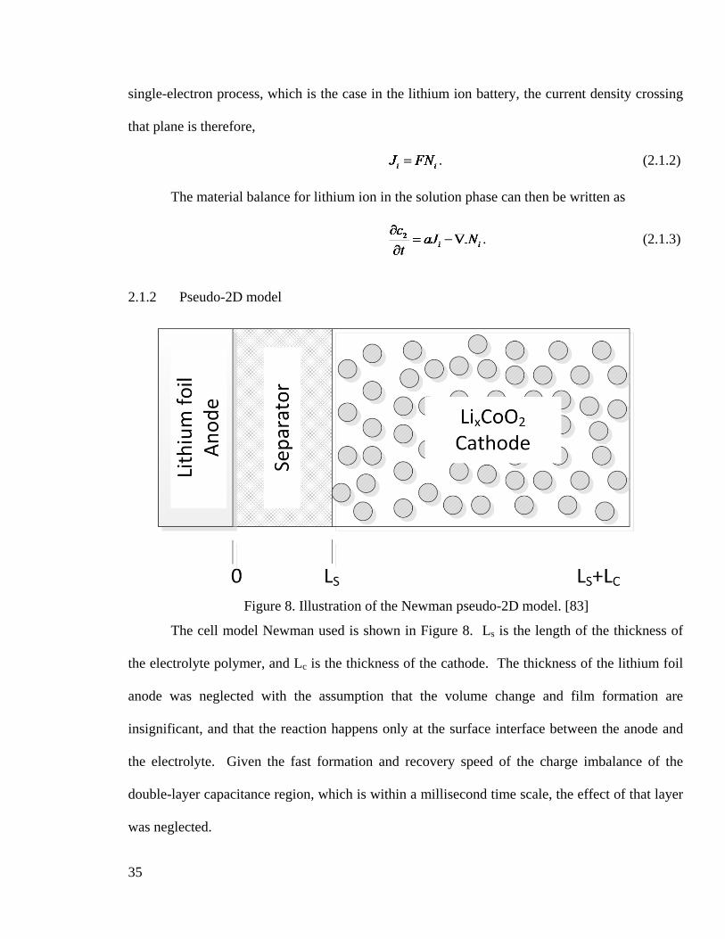
35
single-electron process, which is the case in the lithium ion battery, the current density crossing
that plane is therefore,
. (2.1.2)
The material balance for lithium ion in the solution phase can then be written as
. (2.1.3)
2.1.2 Pseudo-2D model
Figure 8. Illustration of the Newman pseudo-2D model. [83]
The cell model Newman used is shown in Figure 8. Ls is the length of the thickness of
the electrolyte polymer, and Lc is the thickness of the cathode. The thickness of the lithium foil
anode was neglected with the assumption that the volume change and film formation are
insignificant, and that the reaction happens only at the surface interface between the anode and
the electrolyte. Given the fast formation and recovery speed of the charge imbalance of the
double-layer capacitance region, which is within a millisecond time scale, the effect of that layer
was neglected.
36
The general mechanism for discharge involves the oxidation of lithium at the anode, and
the transportation of the lithium ions across the separator into the cathode region. At the cathode
region, the ions are transported into the solid matrix of the cathode material through insertion,
reduced, and embedded within that matrix. The model mostly involves two regions of interest,
the separator (electrolyte region), and the insertion cathode region; the specifics pertaining to the
mechanisms involved in each of these two regions will be discussed in the following section.
2.1.2.1 Electrolyte region (Separator)
The separator consists of a binary electrolyte and a single-phase polymer solvent. At the
concentration levels found in a battery, concentrated solution theory has to be applied. In
concentrated solution theory, the driving force for mass transfer is the gradient in
electrochemical potential, the electrical conductivity, the transference number and the diffusion
coefficient of the lithium salt which characterize the transport in the polymer. Each of these
properties is concentration dependent.
Since only diffusion and migration happen in the separator region, a material balance
equation can be formed,
0
2 22
c tD ct z v F
+
+ +
∂ ∇= ∇⋅ ∇ −
⋅∂
i (2.1.4)
where D is the diffusion coefficient of lithium ion, c is the concentration of the lithium ion, i2 is
the current density and 0t+ is the transference number of lithium ion. z+ and v+ are the charge
number and the number of cations and anions into which a mole of electrolyte dissociates. For

37
the cell, both numbers are 1. Given the lack of reported data, the diffusion coefficient was taken
to be constant, and the transference number was fitted to the formula reported by Newman [83].
0 40.0107907 1.48837 10t c−+ = + × (2.1.5)
The boundary condition for the transport process is affected only by the input flux of the
lithium ion, which is governed by the current applied through the cell via Faraday’s Law. The
relationship is given by,
INF+ = . (2.1.6)
The potential variation across the separator can be calculated from thermodynamic
principles, which gives the relationship,
0
2 lns tI RT cF n z
φκ ν ν
+ +
+ + +
∇ = + + ∇
(2.1.7)
where φ2 is the electrical potential and κ is the conductivity of electrolyte. Other variables
have been defined in the nomenclature at the end of the document.
2.1.2.2 Cathode region (insertion electrode)
The cathode is modeled with two phases, the inert electrolyte, identical to the separator
region, and the solid active electrode. The two phases are superimposed on each other and are
continuous. There is a current carried in each phase. The solid active electrode is modeled as

38
spherical particles of a fixed size which occupy a certain volume of the electrode given by the
volume fraction.
Conservation of Li-ion in the electrolyte phase of this region, accounting for the volume
fraction and the absorption into the solid insertion particle gives,
( ) ( )002 2
eff 2
1naj tc tD ct z v F v
++
+ + +
−∂ ⋅∇= ∇⋅ ∇ − +
∂
i (2.1.8)
where ε is the volume fraction of the electrolyte, and Deff is an effective value for the diffusion
coefficient modified to accommodate the shorter free path length of the species,
0.5effD D= (2.1.9)
The third term in the material balance equation accounts for the absorption of lithium ion
into the solid particles, and jn is defined as the pore wall flux across the interface, and is averaged
over the interfacial area between the solid particle and the electrolyte. This third term exists
specifically to turn a 3-D model into a 1-D macro-homogeneous model. It is the term that will
be discarded later and re-formulated in the modified pseudo-3D model. jn in the above model is a
scalar and is related to the divergence of the current flow in the electrolyte phase, that is i2 from
the following relationship given by Newman,
2i
nsaj i
nF−
= ∇⋅ (2.1.10)
where si is the stoichiometric coefficient of species i, in this case lithium, in the electrode
reaction. si is therefore equal to 1. i2 is defined as the current flow in the electrolyte phase.
The current is based on the transport mechanisms, and is given by the equation,

39
0
2 eff 2 eff 2lns tRT cF n
iz
κ φ κν ν+ +
+ + +
= − ∇ − + ∇
(2.1.11)
where κeff is an effective value for conductivity accounting for the actual free path length of the
species.
1.5effκ κ= (2.1.12)
This “effective” term is also a compensation term for the macro-homogeneous model
which will be discarded. The second phase in the cathode is the active insertion material. This
phase is modeled as spherical particles of radius Rs and the insertion mechanism for the lithium
ions is modeled to be diffusion. Given this assumption, the diffusion can be modeled by the
continuity equation in spherical coordinates,
2
2
2s s ss
c c cDt dr r r
∂ ∂ ∂= + ∂ ∂
(2.1.13)
where cs is the concentration of lithium in the solid particle phase along the x-axis. The diffusion
coefficient Ds is assumed constant in the solid phase.
The boundary condition at r = 0 is,
0scr
∂=
∂ (2.1.14)
and rate of diffusion into the surface is related to the pore wall flux. Hence, the boundary
condition at r = Rs is,
sn s
cj Dr
∂= −
∂ (2.1.15)
Since the two phases are super-imposed on each other, there is one last boundary
condition at the edge of the 1D model, where the flux of the lithium ion must be zero.

40
0 @ i s cN x δ δ= = + (2.1.16)
The reaction rate at the boundary is given by a Butler-Volmer type reaction mechanism,
dependent upon all four state variables, the concentration of lithium ion in the solid phase and
the electrolyte phase and the potential of the lithium ion in the solid phase and the electrolyte
phase.
( ) ( ) ( )' '2 ( ) exp expc a a c
max s T sF Fi Fk c c c c U c c U
RT RTα α α αη η
= − − − − − (2.1.17)
In Newman’s papers, all of the equations mentioned above would then be solved
simultaneously for each point on the x-axis using a customized subroutine in 1D. With the
advancement of finite element analysis tools and advanced solvers, this is no longer required.
2.1.3 Single particle model
While the full model developed by Fuller and Newman [84] is flexible and generalized
for Li-ion batteries with different materials and physical configuration, the complexity incurs
significant time penalty in simulations. Zhang et al. developed a simplified model by assuming a
constant solid phase diffusion coefficient [96] and a uniform concentration distribution of the
lithium ions in the electrolyte phase along the x-axis of the cell. By doing so, it has effectively
abstracted each electrode with porous electrode theory with a single particle (sphere), and hence
the naming of this model.
Under low current condition, the model can be fairly accurate since the concentration
gradient of the lithium ions in the electrolyte phase is minimal. However, the model breaks down
poorly at medium to high current, which limits its use as a comprehensive and complete model.
41
2.1.4 Using COMSOL for simulation
COMSOL Multiphysics® is a finite element analysis, solver and simulation software
platform, based on advanced numerical methods, for modeling and simulating physics-based
problems. With COMSOL Multiphysics, coupled or multiphysics phenomena in different fields
can be solved. It has dedicated physics interfaces and tools for electrical, mechanical, fluid flow,
and chemical applications.
Developed originally from MABLAB based codes for a graduate course at the Royal
Institute of Technology (KTH) in Stockholm, Sweden, COMSOL is now a multi-national
company and the platform is used worldwide for many applications.
COMSOL has three major components, the model geometry builder, mathematical
solvers and an advanced post-processing data visualization module. It is also capable of
importing popular CAD software geometry directly into its solver interface.
The major advantages in choosing COMSOL for this research is three-fold:
1. Speed and reliability: the ODE solvers in COMSOL are based on MATLAB,
which have been tried and proven to be both efficient and accurate. Other
researchers in lithium-ion battery modeling have also reported results based on
COMSOL simulations. [88] [97]
2. Flexibility: COMSOL can accommodate multi-domain models with cross-linked
physics, which is required in the aforementioned lithium ion battery model. The
ability to fully specify and modify the model provides the flexibility to modify the
research scope quickly and with relative ease.
3. Relative simplicity: This research focuses primarily on the application level
strategy for the energy management of a lithium ion battery based on fundamental

42
electrochemistry. The interactive and comprehensive interface allows for a
relatively simple construction of the battery model, without the need for
specialized coding for finite element meshing and solvers, eliminating potential
errors and reducing development time.
For this thesis, all of the simulations were performed with COMSOL Multiphysics®
version 3.5a 64-bit on a PC with the Microsoft® Windows 7® operating system. The PC has an
AMD Phenom X8 64-bit processor, 16 Gb of RAM and all storage drives are SSD based.
2.1.5 Limitations
As with any platform that aims to provide a wide application base for solving physics and
engineering problems, COMSOL is versatile and highly flexible. However, with the automation
in its numerical solver, the solving process is less transparent. The software compensates this
with a running log on the solving process, but failure modes are not clearly identified and can be
difficult to debug.
In the context of this thesis, while COMSOL is very proficient in solving the multi-
domain problem related to the electrochemistry of the lithium ion battery, it was not specifically
equipped to work with its mode of operation.
The typical usage of the lithium ion battery involves three states: discharging, constant
current charging and constant voltage (top up) charging. Translating to the model, each of these
three states requires a different boundary condition at the positive electrode’s current collector,
and switching between the states is governed by a controller that measures the cell’s terminal
voltage and current. COMSOL can be easily configured to change boundary conditions based on
a time-step, but it is not equipped to handle a dynamic switching of boundary condition based on
a changing cell parameter.

43
This dynamic switching is essential to the simulation of this research and a method to
implement it was developed. This will be discussed in detail in Chapter 3.
2.2 Low discharge current model development
In a static fully charged state, both electrodes are protected by a passivating film, which
prevents electrolyte decomposition via redox reactions under a meta-stable condition. At low
current discharge rates, there exists a situation where the passivation layer is weakened, while the
electrodes maintain the highest redox reactivity. It was concluded by Adany et al. that it is
optimal for the discharging current to be sufficient to bring the cell into a partially charged state
[98].
Based on the degradation mechanisms described above for both high current and low
current discharge, it is logical to see that there exists an optimal current, and that its
determination can be based on first principles with semi-empirical experimental data fitting.
Prior work referenced in the previous subsections generally focused on creating a flexible model
to simulate charge and discharge behavior of the cell, and the determination of the physical cell
parameters that continue to change during the continued cycling of the cell via data fitting
methods. The generalized first-principle model [4] attributed all the capacity loss to the anode
and only during charging. While using data fitting, that model can provide some information on
some aspects of the cell during cycle, such as the relationship between EODV to capacity fade, it
does not provide information in space and time for both electrodes, information that is required
to determine the optimal discharge conditions.
This study expands upon the existing model to include both electrodes and it is applicable
to both charge and discharge, even though this study focuses on the discharge cycle. The 2-tier
multi-timescale model developed allows for the dissemination of all of the cell variables,

44
including all electrochemical potentials and concentration distributions in both electrolyte and
solid phases. The model accounts for the amount of electrolyte loss in both electrodes with
respect to both time and position. Specifically, the information on potential distribution in time
and space assists in the development of a discharge method based on external stimulus
(switching, which effectively changes the boundary condition in the model) to minimize the
degradation effects in the cell. This allows for the prediction of cell behaviors under different
discharge schemes which directly relates electrical controls to the internal electrochemistry.
The mathematical Li-ion intercalation model that considers mass transport of lithium in
solid phases, mass transport of lithium ions in the solution phase, charge transport in the solid
phases and charge transport in the solution phases is well developed [83] [84]. The
electrochemical reactions, mass transport, and other processes are also well-known [82].
The rigorous pseudo-2D model was selected for its flexibility and the lack of limitations
in all of the current regions. Computing power has also improved in recent years and the
computation time per cycle remains reasonable.
A summary of the base model, the modeling parameters of the 18650 cell and the
processes described above is described next. The research goal is not to produce an entirely new
model for the cell, but to determine an optimal operating current for application level electrical
design.
To model the low current degradation effects, the electrochemical reaction considered
was the two electron reduction process expressed by Ning [99] while the cell is in its charged
state. At zero discharge current, the cell is at its maximum reduction ability but the reaction is
hindered by the protecting passivation layer. At low current, the passivation layer is weakened by
the current flow, but the reduction potential remains close to maximum.

45
In order to predict degradation reaction rates for a cell that has already been cycled, initial
conditions can be altered in the model. Three parameters have been identified to fluctuate as the
cell is cycled, namely the beginning SOC of both electrodes (x0,pos, x0,neg) and the volume
fraction of the cathode (εpos). The beginning SOC at the cathode and anode increases and
decreases respectively, indicating a lower charge level and a decrease in active material. The
volume fraction at the cathode also decreases as the cell cycles, which also shows a loss of active
material available for cycling. The change of these three parameters with cycling is shown in
Figure 29.
Figure 9. The change of initial values of model parameters with cycles.
The parameters used for simulation in different cycle are shown in Table 2.
-0.1
0
0.1
0.2
0.3
0.4
0.5
0.6
0.7
0.8
0.9
0 100 200 300 400 500 600 700 800
Para
met
er v
alue
s
Cycles
x0,pos
x0,neg
εpos

46
Table 1. Cycling parameters used in the study.
Cycle x0,neg x0,pos εpos
0 0.82 0.200 0.34
100 0.70 0.300 0.30
300 0.53 0.332 0.19
It has been observed that at very low (<C/10) discharge rates, Li metal shorts could form
as the cell cycles [100]. These shorts can lead to catastrophic cell failure and become a safety
hazard. The modeling of this short formation process could be performed via a statistical method
based on empirical data, but is not currently incorporated into the model.
The schematic of a lithium ion battery is shown in Figure 9. It consists of the positive electrode,
the separator and the negative electrode. A lithiated organic solution fills the porous components
and serves as the electrolyte.
LixCoO2
CathodeMCMBanode
Sepa
rato
r
Figure 10. Illustration of a the Li-ion cell used in the pseudo-2D model. [5] [88]
The material balance for the Li ions in an active solid material particle is governed by
Fick’s law in spherical coordinates:

47
1, s,2s, 2
1i ii
c cD r
t r r r∂ ∂ ∂
= ∂ ∂ ∂ (2.2.1)
Where i = p or i = n for the positive and negative electrodes respectively. There is no
flux at the center of the spherical particle, that is, when evaluated at r = 0
1,s, 0i
i
cD
r∂
− =∂
. (2.2.2)
.
On the surface of the particle, the flux is determined by the reaction rate of Li ions due to
the electrochemical reaction occurring at the solid/electrolyte interface. Thus for r = Rs,i,
!,s,
ii i
cD J
r∂
− =∂
(2.2.3)
where Ji is the flux of lithium ions moving away from the surface of the spherical
particles. This wall flux is determined by the Butler-Volmer equation,
( )0.5 0.51, ,max 1, ,surf 1, ,surf
0.5 0.5exp expi i i i i i iF FJ k c c c
RT RTη η = − × − −
(2.2.4)
and the over-potential of the intercalation reaction is given by,
1, 2,i i i iUη φ φ= − − . (2.2.5)
The material balance for the binary electrolyte in the liquid phase is given by,
( )2, 2, 0eff , 1i i
i i i i
c cD t a J
t x xε +
∂ ∂ ∂= + − ∂ ∂ ∂
(2.2.6)
where i = p, n and s for the two electrodes and the separator respectively. ai is the
electrode surface area per unit volume of the electrode (volume fraction). At the two ends of the
electrodes on the x-axis, the flux is also zero, that is,

48
2,eff , 0| 0p
p x
cD
x =
∂− =
∂ (2.2.7)
2,eff , | 0
p s n
np x L L L
cD
x = +
∂− =
∂ (2.2.8)
At the interfaces between the two electrodes and the separator, the boundary conditions
are for the concentration of the binary electrolyte and its flux to be continuous.
2, 2,| |p p
p sx L x Lc c− += =
= (2.2.9)
( ) ( )2, 2,| |
p s p sn nx L L x L L
c c− += + = +
= (2.2.10)
eff , eff ,| |p p
p sp sx L x L
c cD Dx x− += =
∂ ∂− = −
∂ ∂ (2.2.11)
( ) ( )eff , eff ,| |
p s p s
s ns nx L L x L L
c cD Dx x− +
= + = +
∂ ∂− = −
∂ ∂. (2.2.12)
The effective diffusion coefficient of the electrolyte in the liquid phase is corrected by
porosity,
bruggeff , ,
ii e i iD D ε= (2.2.13)
where the diffusion coefficient of the binary electrolyte (De,i) is given as
( )( )34.43 54/ 229 5.0 104, 10 10 iT c
e iD−− − − − ×−= × (2.2.14)
The electrical potential in the solid phase is governed by Ohm’s Law,
2
1,eff , 2
ii i ia FJ
xφ
σ∂
=∂
. (2.2.15)
The effective conductivity is determined by
( )eff , ,1i i i f iσ σ ε ε= − − . (2.2.16)
49
The specific interfacial area is calculated by
( )( )s, ,3 / 1i i i f ia R ε ε= − − (2.2.17)
At the end of the positive electrode, the boundary condition for the charge flux is the
current density applied to the cell,
1,eff , 0 app|p
p x Ixφ
σ =
∂− =
∂ (2.2.18)
where Iapp is the current density applied.
The net electron flux at the electrode/separator interfaces is zero,
1,eff , | 0
p
pp x Lx
φσ =
∂− =
∂ (2.2.19)
1,eff , | 0
p s
nn x L Lxφ
σ = +
∂− =
∂ (2.2.20)
.
The potential φ1 at the edge of the negative electrode is set to zero, and the potential at the
edge of the positive electrode is Ecell, the cell voltage.
The charge balance in the liquid phase is given by,
( ) ( )0
2,eff , eff ,
2 1 lni ii i i i
RT t ca FJ
x x F x xφ
κ κ+− ∂ ∂ ∂ ∂− + = ∂ ∂ ∂ ∂
(2.2.21)
The effective conductivity of the binary electrolyte depends on the temperature and the
concentration of the binary electrolyte in the liquid phase:
bruggeff ,
ii i iκ κ ε= (2.2.22)
where the expression of the ionic conductivity for the electrolyte is given as

50
23 6 24
5 10 2 5 2 8 2
10.5 0.688 10 0.494 10 0.07410
1.78 10 8.86 10 6.96 10 2.80 10i i
i ii i i
c c Tc
c T c T T c Tκ
− −−
− − − −
− + × + × + −= × × − × − × + ×
(2.2.23)
At the ends of the cell, there is no charge flux in the liquid phase, therefore,
2,peff ,p 0| 0xx
φκ =
∂− =
∂ , (2.2.24)
p s n
2,neff,n | 0x L L Lx
φκ = +
∂− =
∂ . (2.2.25)
The potential in the solution phase and its flux are continuous at the interfaces of the
electrodes and the separator.
The reference potential of the positive and negative electrodes are approximated by [5]
2 4 6 8 10p p p p pref
2 4 6 8 10p p p p p
4.656 88.669 401.119 342.909 462.471 433.4341 18.933 79.532 37.311 73.083 95.96p
x x x x xU
x x x x x− + − + − +
=− + − + − +
(2.2.26)
( ) ( )n n0.90 15 0.4465 0.4108ref 0.5n n 1.5
n n
0.0172 0.00190.7222 0.1387 0.029 0.2808 0.7984x xnU x x e e
x x− −= + + − + + − .
(2.2.27)
where xp and xn are the state of charge in the cathode and anode respectively.
Solvent reduction and oxidation are the major contribution to the degradation of the
lithium ion battery. The Butler-Volmer expression was used to describe interfacial reaction
kinetics across the electrode/electrolyte interfaces. Since the reaction involves a single electron
and is assumed to be irreversible, it can be described by a Tafel expression for both electrodes,
( )+
+
s Lios c s* *
s Li
exps n
ccJ i a nFC C
α η
= − − (2.2.28)
where the overpotential term ηs is expressed as

51
1 2 ref,s filmn
Φ ΦsJU Ra
η = − − − (2.2.29)
The resistance Rfilm is defined as
( )film SEI PR R R t= + (2.2.30)
where Rp(t) is related to the film formed by
( ) filmP
p
R t δκ
= , (2.2.31)
and the rate of film formation is related to Js by
s pfilm
n p
J Mddt a Fδ
ρ= − . (2.2.32)
The film resistance at cycle N is therefore given by
( )film film 1 p| | |N N NR R R t−= + (2.2.33)
The value of Uref,s is unknown but has been assumed in the literature to be a constant
independent of the state of charge for each electrode, and given the low rate of this reaction, a
pseudo-steady-state is justified. The values of Uref,s will be stated in the subsequent simulations.
2.3 COMSOL implementation
The mathematical model described in Section 2.2 is a multi-scale model. The
superimposed continua and the abstracted electrodes can be implemented in COMSOL using two
sets of geometries. The three regions of the cell, that is, the two electrodes and the separator, are
abstracted mathematically into a 1D x-axis. This is represented in COMSOL as a line with three
segments. The solid phase of the electrodes requires the simulation of the diffusion of lithium in
the radial direction along the x-axis. A 2D geometry, a rectangle, is used for each electrode for
52
this purpose, and the y-axis of the rectangle denotes the radial direction of the solid particles. The
top boundary of the rectangle is mapped to the corresponding x-axis of each electrode.
The concentration of the electrolyte (c2), the potential in the electrolyte (φ2), the potential
in the solid phase (φ1), the degradation film thickness (film) and the pore wall flux (Jn and Jp) are
solved in the 1D geometry. The pore wall flux is then extracted from the 1D geometry and
mapped to the top boundaries of the 2D geometry using COMSOL’s “subdomain extrusion
coupling variables”.
The concentration of lithium ions in the solid phase (c1) is solved in the 2D geometry.
The surface concentration (cs at r = 0) is mapped to the 1D domain via the “boundary extrusion
coupling variables” for each electrode.
The geometry setup is shown in Figure 10.
In addition to the physical parameters, the switch variables that will be introduced in
Chapter 3 are modeled in a separate dummy geometry that is a single dot. These were added to
the model only for calculation purpose since the switches are dimensionless. The details of the
switches are discussed in the next chapter.

53
Separator Positive ElectrodeNegative Electrode
r r
r=R r=R
Jn Jp
C sp.
surf
C sn.
surf
r=0
Figure 11. Geometry and coupling variables between the geometry of the P2D lithium-ion
battery model. The dotted arrows indicate the mapping of the boundaries.
2.4 COMSOL implementation validation
Given its complexity, the implementation in COMSOL was validated against published
model data. The model used in this study drew heavily upon past work by the battery research
group at the University of South Carolina, headed by Prof. Ralph E. White. The South Carolina
group evolved the model and transitioned it for COMSOL applications. Two major parameters of
the model in this study were matched to ensure the accuracy of the implementation in COMSOL
such that the results can be trusted. The first criterion was terminal voltage, the only parameter
that an electrical engineering design can access, and the value that is used most often for a
battery management controller to assess the state of the cell. The other parameter is the
electrolyte concentration (c2) profile across the length of the cell at different times during a
54
discharge. Using c2 as a validation reference is reasonable because it is the only variable that
spans across all three subdomains in the 1-D geometry. The electrolyte also builds up the most
significant concentration gradient and given the number of studies concerning the diffusion
limitation of the lithium ion cells, the amount of available data is also the most concrete.
This study uses the base semi-empirical model by Ramadass and White [5] which has
been validated against experimental data and cited by many other studies. Two models were
reported in [5], both were evolved from the original P2D model developed by Doyle as discussed
in the last subsection. The first model (hereinafter, Model 1) includes the addition of initial state-
of-charge (θn) and film resistance (Rf) corrections based on experimental data. The second one
(hereinafter, Model 2) further includes a correction expression for the diffusion coefficient in the
solid phase (Dsn,N) to account for the reduced diffusivity upon cycling to cycle N. This correction
expression for Dsn,N is
6, 5 exps
n NkD kN
=
where k5 and k6 are fitting parameters based on experimental measurements and data fitting. All
three correction parameters are used in this study. The diffusivity is implemented in the 2-D
geometry as a “subdomain expression”.
The model as implemented in COMSOL in this study was checked against Model 2 using
the same cell parameters with the diffusion coefficient correction. The data from Model 2 was
obtained with a 0.56 C constant current discharge of a charged Sony 18650 1.8 Ah cell. Multiple
cycles were simulated and the data for cycle 1 and 300 are specifically reported here in Figure
11. The model was run twice at both room temperature (25 °C) and an elevated temperature (50
°C) for their studies. Since this study assumes a controlled temperature environment, the 25 °C
data was used. The same cycles were run in the model of this study and the data is slightly offset

55
by +0.02 V to show the close matching. Close examination of the data values showed that the
simulation results are within +/- 2% between the two sets of simulations for both cycles, which
can easily be attributed to the visual data extraction directly from the published paper.
Figure 12. Comparing the output of the cell voltage (φ1) between the COMSOL model
implementation against Model 1. Solid lines represent the current model offset by 0.02 V for
clarity. Dotted lines were extracted from the reported data in Model 2.
Internal modeling parameters were not reported in Model 2. However, Ning [99] from the same
group used Model 1 and extended it to continuously update the film resistance based on side
reaction calculations, instead of data fitting, to study the internal parameters of the cell over the
cycle life of the cell. The physical reactions and the modeling equations were discussed in
Section 2.2. The Ning model (hereinafter Model 3) used the same parameters from the Sony
18650 cell with identical charging regimes and the discharge rate was 0.5 C. The initial state-of-

56
charge for the positive electrode was slightly changed, from 0.5 to 0.48, and the validation of the
model for this study was adjusted to match the initial conditions. The concentration gradient of
the electrolyte c2 in cycle 1 was reported and the model was run for 9,450 seconds to an EODV
of 3.0 V. The data points of Model 3 were extracted visually from the paper and plotted against
the simulation data of this study in
Figure 12. The simulation data has been offset by +2 mol/m3 to show the general shape,
except for the data at 1000 s, for which -2 mol/m3 has been added. The 1000 s data points
effectively overlap the 9490 s data, since the maximum concentration gradient is dependent upon
the discharge current, and for this simulation, it was reached before t = 1000 s.
900
920
940
960
980
1000
1020
1040
1060
1080
0 0.5 1 1.5 2 2.5 3 3.5
Conc
entr
atio
n of
ele
ctro
lyte
(c2)
(mol
/m3
Dimensionless x-axis (anode to cathode)
0s
50s
1000s
9450s
50s
1000s -2
9450s
Figure 13. Comparing the concentration profile of the Li-ions in the electrolyte phase (c2)
between the COMSOL model implementation against Model 3. Solid lines represent the current
model offset by +2 mol/m3 for clarity. Dotted lines were extracted from the reported data in
Model 3.
57
The two models show very good correlation and close inspection of the specific data
points indicates that the error is within +/- 3%, which is a reasonable tolerance based on the
visual extraction of data.
For the Li-ions in the electrolyte phase, it is expected that diffusion is the transport
mechanism in the separator region, which should give a linear gradient. At the two electrodes,
the Li-ions intercalate and diffuse dependent on the local overpotential, which would vary based
on the both the electrolyte potential φ2 and the potential in the solid matrix φ1. It is also expected
that the variable is continuous at the two boundaries between the electrodes and the separator. At
a low discharge rate, φ1 is very flat across the two electrodes due the low Ohmic drop. And since
the overpotential is the difference between φ2 and φ1, it is reasonable to expect that the shape
shown in Figure 13 to resemble the shape in Figure 12.

58
Figure 14. Potential profile of the Li-ions in the electrolyte phase (φ2) at different time.
Another variable of interest is the electric potential φ1 along the two electrodes. Given the
low resistivity of the solid matrix material, it can be expected that φ1 should have fairly flat
profiles across both electrodes at any given time and that the major potential change would be
across the separator region. It can also be expected that as the cell discharges and the state-of-
charge decreases, that φ1 would also decrease. This can be observed in Figure 14.
(V)

59
Figure 15. Electrical potential profile of the Li-ions in the solid matrix phase (φ1) at different
times.
The implementation of the existing model into COMSOL is the major basis of this study.
Based on the validation parameters matched above, it can be concluded that the base model was
implemented into COMSOL accurately.
The ultimate goal in using this model is to extract the time and spatial information of the
degradation parameters within the cell in order to determine an optimal discharge current for the
lithium ion battery cell. Side reaction by-product’s film thickness can be monitored via the
electrolyte loss in both electrodes both in time and in space for both electrodes, providing
information film growth rate and also the spatial distribution of the side reactions. A specific
sample for the anode can be seen in Figure 16. The plot shows the loss of the electrolyte in one
full discharge cycle at 0.5 C at different time. It can be deduced from this that the rate of
(V)

60
electrolyte loss, and hence film thickness growth, decreases in the latter part of the cycle. The
loss of electrolyte is also more severe at the current collector end of the cell by about 8% in
comparison to the separator boundary.
0.00E+00
5.00E-01
1.00E+00
1.50E+00
2.00E+00
2.50E+00
3.00E+00
0 0.2 0.4 0.6 0.8 1 1.2
Conc
entr
atio
n of
ele
ctro
lyte
loss
(mol
/m3 )
x
5s
6000s
12000s
Figure 16. Electrolyte loss at different time in a sample discharge cycle at 0.5 C.
The result above can be explained by observing the variation of the overpotential
controlling the side-reaction in the anode with a time and spatial plot of its variation over one full
discharge cycle. At each specific time, especially during the earlier part of the cycle, the
magnitude of the overpotential is lower nearer the separator than at the current collector
boundary, as seen in Figure 17. As the cell discharges, the overpotential continues to decrease in
magnitude at a fairly uniform rate, which, based on the rate equation for electrolyte loss, explains
the exponential decrease in the electrolyte loss rate. A portion of the rate decrease in time can be

61
seen in Figure 18, where only the result from the first 4,000 s is shown to emphasize the rate
decrease.
Figure 17. Overpotential for side-reaction in the anode in one full discharge cycle.
Through this model, the concentration of lithium ion in both solid and the electrolyte
phases can be monitored. Since the value of φ2 directly influences the overpotential, and it is in
turn, calculated from the concentration of the lithium ion in the electrolyte phase, it can be useful
to investigate the concentration profile such that strategy can be potentially created to shape
those values by controlling the voltage at the terminals. To illustrate the capability of the model,
the terminal current was changed from 1 C to 0.25 C at 750 s in Figure 19 to show both the
transition of the concentration profile in the anode during each boundary condition change, and
the subsequent profile for each discharge current. It is well known that the final concentration
(V)
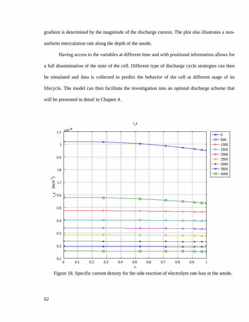
62
gradient is determined by the magnitude of the discharge current. The plot also illustrates a non-
uniform intercalation rate along the depth of the anode.
Having access to the variables at different time and with positional information allows for
a full dissemination of the state of the cell. Different type of discharge cycle strategies can then
be simulated and data is collected to predict the behavior of the cell at different stage of its
lifecycle. The model can then facilitate the investigation into an optimal discharge scheme that
will be presented in detail in Chapter 4.
Figure 18. Specific current density for the side reaction of electrolyte rate loss in the anode.
(Acm
-2)

63
Figure 19. Concentration of lithium ions in electrolyte phase during discharge with a
switching event at 750 s.

64
Chapter 3. Sequential simulation in COMSOL
As mentioned in Section 2.1.4, COMSOL is a versatile platform but it is not equipped to
deal with systems that contain sequential modes of operation based on internally calculated
parameters, such as lithium ion batteries. While COMSOL provides the flexibility to perform
time-domain simulation and time-based modifications of boundary conditions, simulating
sequential systems based on internal physical variables can be a formidable challenge due to the
lack of a built-in method to sequentially change boundary conditions based on calculated
parameters. A lithium ion battery’s charge and discharge cycle has three distinct, sequential
states: discharge, constant current charge and constant voltage charge. The switching between
these three states is determined by the cell voltage reaching specific upper and lower boundaries
as shown in Figure 20.
Discharge Constant Current Charge
Cell Voltage < 3.2 V?
Constant Voltage Charge
Cell Voltage = 4.1 V?
Figure 20. The lithium ion battery discharge/charge cycle, as a three-state, two-switch state
machine.
Depending on the discharging and charging conditions, the time at which these switching
conditions are reached is variable, and simple conditional statement based boundary conditions
would cause switching back and forth between the states due to instantaneous feedback state
chatter. All of these system characteristics and the manner COMSOL is normally configured
directly prevent the simulation of such systems in a straightforward fashion.
In order to overcome this limitation, a systematic, differential equation based approach
that allows the simulation of such sequential state machines was developed. This method makes

65
use of the efficient differential equation solver in COMSOL and while it was originally
developed for this thesis, it can be applicable in other fields. The methodology allows distinct,
digital type one-way switching between states and it is general enough to be adopted for a wide
set of applications.
3.1 Development of sequential simulation method
The initial difficulty with state change in COMSOL is that there is no easy way to
generate a non-time-related step function based on a simple conditional statement using an
internal physical variable. The goal was to create a step-like function based on a physical
variable (in the battery case, the terminal voltage) reaching a specific value, as shown in Figure
21. The x-axis can be time or another independent variable, while the y-axis can be an arbitrary
calculated value based on certain conditions being met.
-2 -1.5 -1 -0.5 0 0.5 1 1.5 2-0.5
0
0.5
1
1.5
2
State 2
State 1
Figure 21. Step function creating a 1-bit two-state change.

66
The monitored variable can have two possible changes after reaching the preset level and
which then changes the boundary condition. It can either reverse its original trend, or it can
continue its trend but at a different rate. In the lithium ion battery case, using the discharge cycle
as an example, the voltage would increase immediately at the end of the discharge cycle and the
current ceases due to the Ohmic drop during discharge. This is shown in Figure 22, at t = 2000.
Figure 22, The lithium ion battery discharge/charge cycle, as a three-state two-switch state
machine
The general steps that this sequential switching in simulation goes through is summarized
in Figure 23. Should a triggering level be set at, say, 3.55 V, using a condition
y = 1 if V < 3.55
y = 0 otherwise

67
would produce a pulse approximately at 1750 < t < 2000. Integrating this pulse would obtain a
Figure 23. Process flowchart for the sequential simulation calculation.

68
step-like function. The condition can be simulated by a Heaviside function
( ) ( )t
-
H t = δ 3.55-V(t) dV∞∫ (3.1.1)
which, in turn, can be simulated in COMSOL via the syntax flc1hs(3.55-V,range). flc1hs is a
smoothed Heaviside function with a continuous first derivative without overshoot. In the interval
–range<x<+range, it is defined by a fifth-degree polynomial. The function with a transition time
at t = 5 with different transition range is shown in Figure 24.
-0.2
0
0.2
0.4
0.6
0.8
1
1.2
0 1 2 3 4 5 6 7 8 9 10
flc1hs(t-5,0.1)
flc1hs(t-5,0.2)
flc1hs(t-5,0.3)
flc1hs(t-5,0.5)
Figure 24. Illustration of the COMSOL smoothed Heaviside function flc1hs with a transition
time at t = 5 and different transition range.
After the pulse has occurred, it is integrated in the time domain to form a step function,
which is then compared to a threshold value. If the step is large enough based on this threshold, a
new boundary condition is sent back to the model for new simulation.

69
3.2 Implementation in COMSOL
The description of the methodology assumes a time-dependent problem with a single
boundary condition to be controlled based on one calculated physical parameter. However, it
can be easily extended to models with multiple changing boundary conditions and multiple
calculated internal physical parameters.
Making use of the fact that COMSOL is an efficient solver for differential equations, the
key concept is to define the behavior of the switching variable through a first-order differential
equation and use the impulse response generated by the computed internal physical parameter
reaching a pre-defined limit and subsequent integration to produce a step-function. This step
function is then used in as a conditional statement in the boundary condition that needs to be
switched.
This base Li-ion battery model was based on the work of Newman as described in
Chapter 2. While this model was developed under COMSOL version 3.5, it is equally applicable
to version 4 of COMSOL using the new interface.
The approach is a four-step process as shown in Figure 25.
Time-based simulation
Determine physical parameter
Create Switch variable in
separate domain
Create Boolean statements for
switching
Implement into corresponding
boundary condition
Figure 25. The four-step differential equation based switching process
Step 1. First, the physical parameters that govern all the switching are defined. In the
example, it is desired that the lithium ion battery switches from discharge mode to charge mode
when the cell potential reaches a 3.2 V lower limit.
Upon reaching the preset cell voltage limit, the boundary condition of an applied current
in this case, is to be changed. The simplified charge and discharge cycle is shown in Figure 26.

70
This is a two-state state machine, and requires only a 1-bit switch. A four-state machine would
require 2-bits, and so on.
Figure 26. The simplified, two-state 1-bit switch, state machine.
Step 2. Having defined the physical parameter, the second step is to assign an arbitrary
variable to be integrated. This variable is then implemented in a unit length subdomain, separate
from the actual physical model. The subdomain’s expression is then set to:
( ) ( )1 3.2 ,0.1 1 50 ,0.1dSwitch flc hs Ecell flc hs Switch ratedt
= − × − × (3.2.1)
where Ecell is the cell voltage, a coupling variable calculated from the physics of the battery.
The first part of the equation provides a smoothed Heaviside step when the switching condition
is met at 3.2 V. If a simple conditional statement is used to create a piecewise function instead of
a smoothed Heaviside function, there would exist a singularity at the transition point and the
simulation would not converge. The second part of the equation sets up an arbitrary upper limit
that the value Switch will attain. The variable rate provides a multiplier to control the speed of
switching. Both the limit and the rate are arbitrary values that can be adjusted for specific
physics. This expression is plotted against time in Figure 27.
Discharge Constant Current Charge
Cell voltage < 3.2 V?

71
Figure 27. Pulse generated by the subdomain expression for Switch.
For this arbitrary Switch variable, all of the boundary conditions in the subdomain are set
to 0 (insulation), with initial value 0.
As the calculated physical value (Ecell) reaches the limit of 3.2 V, the Heaviside function
generates a positive pulse, which is integrated into a step function that is bounded to the high
limit (50 in this case), shown in Figure 28. Since there is no other function to produce a negative
pulse, the value of Switch remains high over time. An “Integral Coupling Variable” IntSwitch
(integral of Switch over the unit length domain) can then be used to carry the step function back
to the physical domain for calculations.

72
Step 3. Using IntSwitch, two distinct Boolean variables can be created as “Scalar
Expressions”.
( ) flc1hs 25 ,0.05Discharge IntSwitch= − (3.2.2)
( ) flc1hs 25,0.1Charge IntSwitch= − (3.2.3)
Figure 28. Pulse integrated to become a non-reversible step function with adjusted
conditions.
The Discharge state is true when the value IntSwitch is less than 25, while Charge is true
when it is over 25. 25 is chosen as the mid-point between 0 and 50. The range in the Heaviside
functions differs intentionally to provide asymmetrical switching time for the two Boolean

73
variables. This is needed to prevent chatter between states, and improve convergence. Note that
this value is only an initial choice for testing purposes in the time-based simulation. It would
likely require adjustments after the implementation of the switch into the boundary condition.
The change in boundary condition will inadvertently causes a change in width of the
pulse and hence the integrated value of Switch.
Step 4. The two variables can then be implemented into the boundary condition. In this
application, the boundary condition is an applied current i_app.
_ _ _i app i discharge Discharge i charge Charge= × + × (3.2.4)
where i_discharge and i_charge are current constants in Amps (A).
It should be noted that upon adding the conditional statement to the boundary condition,
there is now a dynamic feedback in the system and the boundary condition is now independent of
time. This invariably will change the value and the width of the pulse generated by the
Heaviside function in Step 2, which would subsequently produces a value for Switch that may or
may not be bounded by the limit (50 in the example) and that the rate variable should be adjusted
to create a usable step function. In this example, the initial rate created a step function between 0
and just over 1, as shown in Figure 29.

74
Figure 29. New IntSwitch value after implementing conditional applied current into
boundary condition.
To make this usable for the conditional statements, the mid-point was adjusted from 25 to
0.5 for the two Boolean variables.
Discharge=flc1hs(0.5-IntSwitch,0.05)
Charge=flc1hs(IntSwitch-0.5,0.1)
With this adjustment, the setup for the dynamic switching simulation is complete.
In this example,
i_discharge = -i_charge = 17.5,

75
and the applied current boundary condition is shown in Figure 30.
Figure 30. Discharge and charge current based on conditional switching.
Using this boundary condition, the charge and discharge curve was simulated, and the
result is shown in Figure 31.
At time = 2651 s, the current switched within a period of about 10 s. The voltage step
corresponded to the Ohmic drop, and the subsequent increase is due to constant current charging.
The behavior is identical to the time-based simulation. There is a small amount of settling time
within the switching period, but convergence was obtained.

76
Figure 31. Discharge-charge voltage curve based on conditional switching.
3.2.1 Improvements since publication
3.3 Discussions, limitations and improvements
While the four-step process described above involved a single switching event, it can be
extended to systems involving multiple conditions simply by adding more arbitrary "switch
physics" into the unity length subdomain and creating the table of boundary conditions to the
corresponding "logic states". The three steps after the definition provide much needed flexibility
such that each of the switching events can be tailored to fit each specific physical condition. The
size of the impulse function can be adjusted by changing the rate and the Heaviside function's
range variable in the subdomain expression in step 1. The switches can also be customized to fit

77
the output of the integrated step function before it is implemented into the boundary expression
of the physical variable of the model.
It should be noted that the adjustment of the rate and the conditional statement Boolean
variables to obtain proper switching is an iterative process which must be adaptively refined once
the conditions are implemented into the physical subdomain as a boundary condition. This
dynamic feedback also requires that the sequence of the events be considered. The asymmetry of
the switching statements is needed to generate hysteresis, thus producing a one-way and
irreversible change that is free from non-convergent simulation chatter.

78
Chapter 4. Optimal discharge current strategy
In this chapter, an optimal discharge strategy for a lithium ion rechargeable battery will
be presented. Multiple types of existing discharge methods for multi-cell battery packs and the
corresponding pros and cons are discussed in Sections 4.2 and 4.3. The state-of-the-art
theoretical penalty-based discharge method [97] will be summarized and the arbitrary theoretical
minimum penalty optimal current defined in Section 4.4. The following sections will discuss the
method to determine the physical optimal current to maximize cycle life developed in this thesis,
including the results of the simulation and analysis. The conclusions, limitations and potential
future work that can future extend this work will be presented in Section 4.6.
4.1 Introduction
Multi-cell battery packs based on standard 18650 cells have become a standard in energy
storage from laptops to EVs. These packs have multiple advantages, including the flexibility in
configuration for different voltage and current needs and the safety aspect. Using small cells with
smaller amounts of energy, single cell failures will not cause a catastrophic failure in the system.
In terms of safety, the chance of a fire happening due to a single cell failure in a multi-cell pack
is much lower than if the cell is a monolithic pack. Integrating a multi-cell package also
decreases the volume to surface area ratio, allowing better ventilation and thermal control using
fluid cooling (typically a mixture of glycol and water). Redundancy and the flexibility in
implementing different algorithms are also enabled by using multi-cell packs versus a single
monolithic battery. For example, the Tesla Roadster uses 6,800 of the 18650 cells, divided into
11 integrated battery modules [100].
Battery management for multiple battery systems has been widely studied. Most of the
studies were intended to maximize the battery discharge capacity throughout the cycle life of the
79
cells. There are two kinds of discharge algorithms: sequential and parallel. In the sequential
algorithms only one battery supplies the electric power to the load each time, while in the
parallel algorithms a subset of batteries supplies power to the load each time.
Sequential discharging algorithms for lifetime maximization of systems with multiple
identical batteries were proposed and tested by Benini et al. [101]. The proposed algorithms
include: (i) serial discharging each battery until it is emptied and then discharging the next
battery; (ii) discharging each battery for a certain amount of time then moving to the next battery
(static switching); and (iii) discharging each battery for a different amount of time depending on
its physical state, e.g. state-of-charge of each cell, remaining capacity or terminal voltage
(dynamic switching)..
In [101], the lifetime of a multiple battery system was compared to the lifetime of a
monolithic battery, i.e. a single battery with a capacity equal to the sum of all the batteries. Static
and dynamic algorithms were found to significantly increase the life-time and close the discharge
capacity gap compared to a monolithic battery. Following the results of Benini [101], the need
for dynamic algorithms which determine the next discharge schedule based on the cells’ state
was suggested as necessary.
Parallel discharging algorithms, with and without sequential switching, for systems with
multiple identical batteries were discussed by Rao et al. [102]. According to the analytic results
presented, when using parallel discharging algorithms the lifetime of a multiple battery system is
equal to that of a monolithic battery and not less than that when using sequential algorithms. In
addition, Rao et al. reported that the lifetime of batteries operated by any switching algorithm
becomes very similar to that of a monolithic battery, as the switching frequency increases.

80
4.2 Multi-cell discharging schemes
Multiple discharging schemes to improve discharge capacity have been proposed and
experimentally analyzed by Rao [102] et al and Benini [101] et al. All of the methods are based
on the relaxation effect of the Li-ion batteries. If a battery is allowed to rest in between
discharges, it was observed that the total discharge capacity would increase.
A test bed was developed using LabView and a National Instrument DAQ module to
verify the results during the early part of this study. The test bed controlled the charge or
discharge current values and duty cycle.
A Panasonic 18650 Li-ion battery with 1.4 Ah capacity was used. The cell was fully-
charged to an EOCV of 4.1 V through the full CC-CV cycles. The CV cycle ended when the
charge current drops to 20 mA in the CV stage. The cell was then discharged at different duty
cycles using the same discharge current (2 A, which translates to 1.4 C for the particular cell)
while the duty cycle was varied. The x-axis is normalized to show the increase in discharge
capacity in a at different duty cycle, i.e. the time axis was compressed by 2 times for the 50%
duty cycle, and 4 times for the 25% duty cycle. The time period for the pulse discharge was 30
seconds. Using a typical EODV of 2.5 V, the results can be seen in Figure 32 that the discharge
capacity is improved by 28%, which is also in line with other researchers’ observations [101].

81
Figure 32 Normalized discharge curves for a Panasonic 18650 1.4 Ah cell at different duty
cycle.
Experimental results have shown that the discharge capacity using both open and closed
loop multiplexing methods in a multi-cell battery system improves over the sequential
discharging method. Adany [97] et al proposed switching algorithms that select a subset of a
battery’s cells based on demand using an optimized current (IOPT) per cell, at which the penalty
was assigned a value of 0. Deviation from this optimal current will incur a proportionately
increasing penalty. The proposed algorithms were demonstrated to reduce the penalty function,
although the value of IOPT was arbitrarily set. The penalty model was linear for currents both
higher and lower than IOPT. While this assumption of linearized penalty works for simplicity in
simulation, it does not take into account the non-linear degradation elements in the discharging
cycle of a cell. This penalty-based method will be discussed in detail in Section 4.4.
0.00E+00
5.00E-01
1.00E+00
1.50E+00
2.00E+00
2.50E+00
3.00E+00
3.50E+00
4.00E+00
4.50E+00
0 500 1000 1500 2000 2500 3000
Vol
tage
(V)
Time (s)
Discharge 2A Batt1 No Pulse
Discharge 2A Batt1 Pulse 50%
Discharge 2A Batt1 Pulse 25%

82
4.3 Trade-offs between different schemes
4.3.1 Sequential discharge
Other than the simplicity of implementation, sequential discharge does not offer any
capacity advantage, nor minimize degradation. It has been demonstrated that if two batteries at
half the capacity of a monolithic battery are discharged sequentially with identical load, the
discharge capacity is always lower than that of the monolithic battery [104]. This can be
explained by noting that the constant load current has effectively been doubled for each of the
two cells, and while the monolithic cell would follow the discharge curve at 1 C; the half-
capacity cells are discharged effectively at 2 C, which results in less discharge capacity based on
the Peukert’s relationship. Despite the advancement of other algorithms, sequential discharge is
still the most popular discharge algorithm in consumer electronics due to its simplicity in
implementation.
4.3.2 Open-loop Switching (Sequential scheduling)
Open-loop Switching switches the load current from one cell to the next based on a fixed
frequency fsw. It is simple to implement with almost no computing power needed. The two
extreme limiting cases are for fsw = 0, which is the case of sequential discharge; or for fsw = ∞,
which is the case of an equivalent monolithic battery. While choosing very high fsw seems to be
desirable, in practicality, experiments and simulations have shown that increasing the fsw beyond
a few tens of a Hz hardly impacts the increase in discharge capacity. This can be explained by
simulation that relaxation phenomenon occurs in a time frame of seconds, and that higher
frequency would not allow the relaxation to occur. Very high fsw also incurs a penalty in
switching overhead. Switching is not a zero-energy operation, and each switching event includes

83
a finite energy loss. Another limitation to the open-loop switching policy is that it does not take
into account the status of the cell. In a vehicular environment, the load pattern is unknown, and
without more intelligence in the scheduling system, the benefit of the open-loop switching is
questionable.
4.3.3 Close-loop Switching
Close-loop switching uses measured cell parameters to dictate when switching between
cells occur. A simple version typically implemented in some consumer product battery
management solutions uses a threshold voltage at the terminals as the triggering parameter.
While the discharge capacity in general improves, there is the overhead cost of extra sensing
circuitry, memory usage and more complex, and hence more expensive, controller.
4.4 Penalty based system
While the methods described in Section 4.3 are widely deployed in many consumer
electronics applications, the developments and analyses were mostly experimental and loosely
based on the result of the relaxation phenomenon of these lithium ion batteries. For more
expensive and permanent installations like EV, HEV and sustainable energy storage, however,
the demand for longer cycle life is more stringent and there is a need for a more sophisticated
method that explicitly considers the internal electrochemistry of the cells.
The penalty-based discharge algorithm proposed by Adany et al. [97] realized the need
for a cell chemistry-centric approach to discharge in order to minimize long-term degradation.
The following sub-sections provide a detailed description of this system.

84
4.4.1 System description
The system is an abstracted load very similar to the applications in EV and sustainable
energy power supplies. The terms used are summarized in Table 2.
Table 2. Notation and terms summary for the penalty-based algorithm
Cell-series s1, s2,…,sm
C The initial capacity of all cell-series.
ijc The capacity of cell-series j before demand i.
IOPT The optimal discharge current of the cell-series.
Current demands d1, d2,…,dn
di The current demand for the i-th second.
Decision variables
ijI The discharge current of cell-series j for demand i.
A battery pack consists of m identical cell-series, s1, s2,…,sm. All series have the same
initial capacity C. This battery pack would provide the load with n current demands, d1, d2,…,dn
where di is the current demand in amperes (A) for the i-th second. The values of both di and n are
both unknown in advance. The total capacity of the cell-series, however, is guaranteed to satisfy
all demands, i.e. 1
nii
d mC=
≤∑ .
The current demands di and the remaining capacity status ijc of the all cell-series are
given to the switching algorithm every second.
The i-th current demand can be fulfilled in multiple ways. The objective is to minimize
the total penalty of the cell-series and maximize the cycle life of the entire battery pack. There is

85
no restriction in how the demand di is allocated among the cell-series. Thus, the algorithm is
required to determine the value ijI to supply the demand di.
In turn, each allocated current ijI is associated with a penalty, since an optimal discharge
current IOPT exists. The penalty is based on the conclusion that deviation from this optimal
current, either too high or too low, would negatively impact the battery’s cycle life. This penalty,
based on the allocated current, is then aggregated over time. While the accurate penalty function
depends on the specific chemistry and geometry of the cell, some basic assumptions can hold.
1. The penalty at no discharge = 0.
2. The penalty of ijI = IOPT = 0.
3. Other discharge currents have positive penalty proportional to the distance from
IOPT.
This simplified penalty function can be written as
OPT
OPT
0, if ( )
else for 0I I
Penalty II I Iα
== − >
where α > 0 and is a proportional constant.
The penalty function is presented in Figure 33.

86
Figure 33. The penalty function per Adany et al. There is a specific discontinuity at I = 0,
where the penalty is 0. [97].
The mathematical model to minimize the penalty function is therefore written as follows.
( )1 1
1
1
min
such that 1...
1...n
0 , 1... , 1...
n mij
i in
ij
im
ij i
ii ij j
Penalty I
I C j m
I d i
I I R j m i n
= =
=
=
≤ ∀ =
= ∀ =
≤ ∈ ∀ = =
∑∑
∑
∑
The first constraint ensures that the cell-series j possesses enough capacity. The second
constraint requires that the demand di is satisfied by the discharges of the cell-series. The last two
constraints ensure that ijI is real and non-negative.
Based on this penalty function, Adany et al. proposed multiple algorithms and compared
the penalty value to the most commonly used discharge method in EV today, which is to supply
Well reported/studied
Not well studied/ modeled

87
the current demand by dividing the load equally between all cell-series. It was reported that the
penalty was minimized by 50-90% depending on the simulation data used and that most penalty
occurred at the end of the discharge cycle for most of the cell-series. It was also observed that
increasing the number of cell-series in parallel reduces the penalty even further.
4.4.2 Limitations in the theoretical penalty based model
There are multiple assumptions in the penalty model that would prevent it from being
implemented.
First, it assumes that all the cells have a flat voltage profile. With the current
advancement in cell chemistry, particularly the graphite LiFeO4 type cells, this is a fair
approximation. However, this assumption implies that the half-cell potential on both electrodes
remain the same throughout the discharge cycle, and this further implies that the degradation
mechanisms associated with each electrode are fairly constant as well. As has been discussed in
Chapter 2, this is not the case in a physical battery.
The linear nature of the penalty model assumes that the degradation mechanisms for high
discharge current and low discharge current share very similar reaction rates or that the effect on
the battery’s life cycle are identical. This assumption is highly inaccurate due to the fact that the
degradation mechanisms involved at these different current ranges are different, particularly in
the mechanisms involving abrupt volume change and physical damages due to extremely high
intercalation rate. There is also no theoretical or experimental basis for the linear increase in
penalty on either side of the optimal current as well.
Lastly, the theoretical optimal current IOPT is arbitrarily assigned in the model and is
assumed constant. The authors further suggested that the value should be obtained
experimentally. While the high current degradation effects and mechanisms are well researched,

88
the low current degradations have so far only been experimentally observed. There is a lack of
modeling work that describes the degradation mechanisms associated with low current discharge
and this is the major contribution of this thesis.
4.5 Determination of the optimal current (IOPT)
4.5.1 Analysis methodology
The effect of different degradation mechanisms on the operating parameters have been
well documented [77] and discussed in Chapter 1. Loss of electrode materials, associated with
high discharge rate, modifies the state of charge (SOC) on both electrodes, while electrolyte
decomposition results in a reduction in the effective diffusion coefficient in the solution phase.
The side reactions are extremely slow relative to the rate of ion intercalation, and the cell
parameters can be assumed to be in a pseudo-steady-state in each cycle. Different side reaction
mechanisms can also be isolated by the corresponding operating current range. As stated in both
Chapter 2 and Section 4.4.2, the degradation effects associated with high current discharge is
well researched. This section looks specifically into the low current degradation mechanisms.
Combining the new results with results in the existing literature, the trend of the optimal current
can be determined.
The contribution to the overall capacity fade from each degradation mechanism is
indirect. In this model, the effect of each degradation mechanism is quantified by isolating its
specific effect, and its effect on the discharge capacity per cycle is recorded. Instead of keeping
the depth of discharge (DOD) constant, the amount of charge passed through the cell per cycle is
kept constant to isolate the effect of material loss, i.e. a 0.5 C discharge would be run for twice as
long as a 1 C discharge. Accounting for a fixed amount of charge is also helpful at the
application level in the design of fuel gauge and charge controllers.

89
Given that the initial film formation process and conditioning are performed by the
manufacturers, which are also inevitable, the parameters used in the beginning of the model
represent the values after conditioning. Parameter fitting was performed based on reported
parameters at different cycles to determine the shift in the optimal current. The degradation
reactions for low current degradation are the redox reactions due to the weakened passivation
layer. These have been reported as a two-electron process [98] and have been discussed in detail
in Chapter 2. The reactions can be summarized as follows.
EC + 2e- + 2Li+ → LiCH2CH2OCO2Li for anode reduction,
ClO4- ClO4 + e- → ClO2 + 2 Oad + e-
ClO2 + H+ + e- → HCl + O2 for cathode oxidation,
and the calculation in material loss has taken that into account.
In order to correlate the result to the aforementioned multiplexing type discharge scheme
in a multi-cell pack, the discharge rates were chosen to be fractions of the C values.
Other general modeling parameters for the 18650 cell are shown in Table 3.
Table 3. Parameters for the cathode and anode materials.
Symbol Units Anode Cathode
Li μm 88 80
σeff S m-1 5.76 12.117
ε2 0.485 1.385
cmax mol m-3 30555 51555
D1 m2 s-1 3.9 x 10⁻¹⁴ 1.0 x 10⁻¹⁴
k (A m-2)/(mol m-3)3/2 2.2 x 10⁻⁶ 9.81 x 10⁻⁷

90
αa 0.5 0.5
αc 0.5 0.5
c02 mol m-3 1000 1000
D2 m2 s-1 7.5 x 10⁻¹⁰ 7.5 x 10⁻¹⁰
t+ 0.363 0.363
R0f Ωm2 0.01 0
Uref,s V 0.38 3.8
4.5.2 Results and discussions
The profile of the loss of electrolyte for the cathode at the end of Cycle 1 is shown in
Figure 34. The x-axis is dimensionless and is not proportional to the size of the electrodes and
the separator. The thicknesses of the electrodes and the separator are abstracted into the
corresponding equations. The length of the anode is shown in the plot from 0 to 1, the separator
from 1 to 2, and the cathode from 2 to 3. The amount of electrolyte loss along the cathode is
relatively constant from the separator/electrode interface and drops near the current collector
with some irregularity. Since the purpose of this analysis is to establish the strategy for effective
discharge based on external control of the cell, for consistency, the data points for the loss of
material in the cathode are taken at x = 2.5.

91
0.00E+00
1.00E+00
2.00E+00
3.00E+00
4.00E+00
5.00E+00
6.00E+00
7.00E+00
8.00E+00
9.00E+00
2 2.1 2.2 2.3 2.4 2.5 2.6 2.7 2.8 2.9 3
Conc
entr
atio
n of
ele
ctro
lyte
loss
(mol
/m3 )
Normalized distance
0.25C
0.33C
1C
Figure 34. Concentration loss plot against the normalized length of the cathode after Cycle
1.
4.5.2.1 Single-Cycle Optimization
Figure 35shows the concentration of solvent loss after the first discharge cycle (Cycle 1)
at the cathode at different current levels. The shape of these plots remains very similar to each
other with a relatively flat rate of loss due to the side reaction. This loss rate increases slightly
toward the end of the discharge cycle. Since the end of each plot represents the same discharge
capacity, it can be seen that as the discharge current decreases, the total electrolyte loss increases.
At 0.5 C, the total loss of electrolyte at the cathode increases by 1.72 times over the loss at 1 C.
At 1/3 C, 2.38 times, and at 1/4 C, 2.97 times. The rate of loss between different discharge
currents is very similar for the cathode during the first part of the discharge cycle, and the
deviation in the later stage is also fairly small. This indicates a primarily time-dependent process.

92
0.00E+00
5.00E-02
1.00E-01
1.50E-01
2.00E-01
2.50E-01
3.00E-01
0 2000 4000 6000 8000 10000 12000 14000
Conc
entr
atio
n of
ele
ctro
lyte
loss
(mol
/m3 )
Time (s)
1C
0.5C
0.33C
0.25C
Figure 35. Concentration of electrolyte loss at the cathode after one cycle at Cycle 1 at
different low discharge rate.
Figure 36 shows the concentration of solvent loss after the first discharge cycle (Cycle 1)
at the anode at different current levels. As with the cathode side, the total loss of electrolyte
increases as the discharge current drops. However, it is clear that the rate of loss levels off and
there are two distinct regions. This two-region behavior shows that the strategy to minimize the
low current degradation should be based on the reaction at the anode. The rate of loss is very
similar among all plots in the first stage before the flat region, and that the 1 C discharge reaches
the low loss second region almost as quickly in the absolute time-scale. All four discharge cycles
reach 90% of the maximum electrolyte loss, a point chosen for consistency as well as being
indicative of the state of the cell as the rate of loss decreases to almost zero, when the SOC of the
anode reaches approximately 0.62. The amount of degradation and that the anode is the dominant

93
limiting electrode are in general agreement with the finding of Zhang [77]. The nature of the
degradation in the anode is consistent with the observation of Ning [76] and the hypothesis of
Adany [97] as well.
0.00E+00
1.00E+00
2.00E+00
3.00E+00
4.00E+00
5.00E+00
6.00E+00
7.00E+00
8.00E+00
9.00E+00
0 2000 4000 6000 8000 10000 12000 14000
Conc
entra
tion o
f ele
ctro
lyte
loss
(mol
/m3 )
Time (s)
0.25C
0.33C
0.5C
1C
Figure 36. Concentration of electrolyte loss at the anode after one cycle at Cycle 1 at
different low discharge rate.
It can be deduced based on the shape of the plots, that the initial optimal discharge
current can be as high as 1 C in the beginning of each cycle as the rate of loss is similar at
different current levels. As the cell approaches the SOC at which the low current related
degradation loss has slowed, reducing the discharge current would decrease the amount of
degradation caused by physical damage discussed earlier, while the degradation caused by low
current related processes has tapered off. The discharge current in the second region can be
Stage 1
Stage 2

94
safely reduced to 0.25 C. This shows that if the penalty-based model is used to optimize the
cell’s cycle life by minimizing long-term degradation, the zero-penalty current (IOPT) is, in fact,
not a constant, and should decrease as the SOC of the cell discharges. However, the linear
properties suggested by the penalty-based model for low current are justified by the almost
inversely proportional nature of the loss of electrolyte against discharge current level.
4.5.2.2 Optimization over discharge cycles
The rate of electrolyte degradation loss decreases as the cell cycles. Three specific cycles
are shown in Figure 37. This can be explained by the Ohmic resistance caused by film formation
and the decrease in initial SOC, which reduce the reduction potential at the anode and the rate of
electrolyte dissociation.
Figure 37. Electrolyte loss at 1 C discharge rate at three different discharge cycles.
0.00E+00
2.00E-01
4.00E-01
6.00E-01
8.00E-01
1.00E+00
1.20E+00
1.40E+00
1.60E+00
0 500 1000 1500 2000 2500 3000
Conc
entr
atio
n of
ele
ctro
lyte
loss
(mol
/m3 )
Time (s)
Cycle 1
Cycle 100
Cycle 300

95
The SOC for both electrodes just before the flat region in Figure 36 were within 1% of
each other for all discharge current per cycle. The SOC values at 90% of the maximum loss for
both electrodes are presented in Figure 38. As the cell cycles, the beginning SOC for both
electrodes change based on Figure 9, and the difference between the beginning SOC and the
90%-level SOC continues to decrease. In Cycle 1, the change in SOC in the anode from the
beginning of cycle to the second region is -0.2, while in Cycle 300, this change has dropped by
half to -0.1. A similar conclusion can be drawn from the SOC at the cathode.
The decrease in the change of SOC to reach the low loss region is indicative of a shorter
discharge time to reach the flat second region at the anode, which is shown in Figure 39. The full
discharge time for different discharge currents were different but the percentage of the time
0
0.1
0.2
0.3
0.4
0.5
0.6
0.7
0 50 100 150 200 250 300 350
Stat
e-of
-cha
rge
Cycle
State-of-Charge (Anode)
State-of-Charge (Cathode)
Figure 38. Variations of SOC at the 90%-loss level at the cathode and anode with cycle
number.

96
period to reach the flat region is consistent. As the cell cycles, the percentage of the discharge
time it requires to reach the low loss condition is almost halved, from 32% down to 16% in
Cycle 300. Given that the degradation rate at the lower discharge current region in Cycle 300 is
less than 10% of the rate in Cycle 1, together with the strong evidence from other studies that
high current degradation effects diminish significantly below 1 C, the optimal current at the
beginning of each cycle should decrease as the cell cycles. The need to reduce this optimal
current within each cycle is no longer as crucial as it was at a lower cycle number.
0.00%
5.00%
10.00%
15.00%
20.00%
25.00%
30.00%
35.00%
0 50 100 150 200 250 300
% o
f dis
char
ge t
ime
befo
re 9
0% lo
ss i
s re
ache
d
Cycle
Figure 39. Percentage of discharge time elapsed to reach 90% of maximum electrolyte loss
per cycle.
4.6 Summary of observations
Based on the results in section 4.5, the following trends can be observed.

97
1. There are two distinct stages for the degradation reaction in the anode, and the
transition happens at approximately the same SOC regardless of the magnitude of
the discharge current.
2. The amount of electrolyte loss due to low current degradation decreases as the
cycle number increases.
3. The difference between the beginning SOC and the 90% corner SOC at the anode
decreases as the cycle number increases.
4. The time required to reach the flat, no degradation region decreases as the cycle
number increases.
5. The electrolyte loss at Cycle 300 is less than 10% at Cycle 1 at the same discharge
current rate.
6. As discharge current decreases, the degradation level based on high current
degradation mechanism decreases.
7. As the discharge current decreases, the degradation level based on low current
degradation mechanism increases in the beginning of the discharge cycle.
4.7 2-Stage discharge method
Combining the results in 4.5.2 and the results from published literature, it was observed
that a 2-stage discharge method could achieve an optimal discharge capacity per cycle while
minimizing the level of degradation of the cells. The goal of this method is for the cell to reach
the specific state-of-charge at which the low current degradation tapers off as quickly as possible
without triggering the high current degradation mechanisms.
This method assigns two different IOPT to the battery cell while implementing the penalty
based switching algorithm at the two different stages in the discharge cycle, as discussed in the

98
last section. From its fully charged state, the IOPT in the first stage is in the intermediate discharge
current region, a value that would abide by the second constraint that this current would not
significantly trigger high current degradations. As the cell reaches Stage 2, the discharge current
would decrease to a low current discharge level, but not low enough that could trigger shorts
formation. The method requires the monitoring of the state-of-charge of the cells and the
knowledge of the right state-of-charge point to switch between the two stages. The difference in
the initial state-of-charge and the switching state-of-charge is also needed as the cell cycles.
0
0.2
0.4
0.6
0.8
1
1.2
0 1000 2000 3000 4000 5000 6000 7000 8000
Disc
harg
e cu
rren
t (C)
Time (s)
Discharge current (C)
Stage 1
Stage 2
Figure 40. Discharge current profile for an 18650 cell with a switching time at 572s.

99
The switch to the lower Stage 2 current is based on the fact that the lower discharge
current would create significantly reduced degradation based on high current related
mechanisms. As discussed in Chapter 1, the level of degradation incurred by the high currents is
significantly higher than those at both the intermediate current level and the level of degradation
in Stage 1 at low current. Lower discharge current reduces the discharge temperature of the cell,
effectively lowering all reaction rate of degradations, and reduces the mechanical shock that
would be experienced by the electrodes.
0
0.1
0.2
0.3
0.4
0.5
0.6
0 1000 2000 3000 4000 5000 6000 7000
Stat
e of
char
ge
Time (s)
Stage 1
Stage 1
Figure 41. State-of-charge decreases in the anode at two different rate based on the 2-Stage
discharge method. The switching time depends on the state-of-charge corresponding to the time
at which the anode low current degradation tapers toward zero.
The lower Stage 2 current is also able to avoid triggering the low level discharge current
degradation in the anode since the overpotential of that reaction has dropped to a point where the
rate is negligible. Besides, given that Stage 2 runs for a significantly longer time period than

100
Stage 1, the discharge capacity would likely increase and follow the lower discharge current’s
discharge curve. The method is illustrated in Figure 40.
Using one of the discharge curves from the Sony 18650 cell as an example, the beginning
current level is set at 1 C, which is an intermediate discharge current that is recommended by the
manufacturer. Any current higher than this level would incur significant degradation. However,
discharging at 1 C would allow the cell to reach its switching state-of-charge of 0.62 relatively
quickly compared to lower currents. In this case, the changeover time was 572 s, while the full
discharge time was 5971 s. The change in the state-of-charge throughout the discharge cycle is
shown in Figure 41.
IOPT2
Pena
lty
Discharge current
α2IOPT
Figure 42. Modified Penalty curve for the discharge current in Stage 2.

101
4.8 Application of the 2-Stage discharge method
The 2-Stage method was developed to be applied in conjunction with the penalty based
switching method described in Section 4.4. This method modifies the initial assumption of the
penalty model into two distinct stages. The first stage (Stage 1) follows that penalty curve
initially suggested by Adany, shown in Figure 33, and now has a framework to determine the
value of IOPT and the linear penalty approximation has been tested to be accurate on the low
current side. In Stage 2, two changes from the Stage 1 curve are made. The IOPT is revised down
to a lower value, one that would significantly reduce the high current degradation reactions but
not too low (< 1/10 C) as to potentially causing lithium metal dendrite formation. The second
change is the reduction of the slope to the left of IOPT. Simulation results have shown that the rate
of low current degradation after the specific state of charge value has been met all taper toward
zero and the loss of electrolyte becomes flat. The similar in side reaction rate would suggest a
lowered penalty value as the discharge current is reduced. This Stage 2 modified curve is
illustrated in Figure 42.
4.8.1 18650 application test case
The 2-Stage method was applied to the popular Sony 18650 cell in a test case to illustrate
its performance. The cell under test begins as a fully charged cell and it is subsequently
discharged to the EODV of 3 V. Three discharge methods are used for comparison.
1. Constant current at 1 C continuously.
2. Constant current at 0.25 C continuously.
3. 2-Stage discharge with 1 C in Stage 1, and 0.25 C at Stage 2.
Two parameters of application level importance were observed, namely the per cycle
discharge capacity and the amount of loss of electrolyte. The loss of electrolyte affects the

102
discharge capacity indirectly by a reduction in the diffusion coefficient which results in a slightly
higher internal resistance as observed at the terminals. However, this effect is minute given the
small amount of per cycle degradation that occurs. Hence, the best way to compare the amount
of degradation caused by low current degradation mechanism between the three cases would be
to look directly at the electrolyte loss, since this value is cumulative over the cycle life of the
cell.
As the cell cycles, the cell parameters would change and the switching state-of-charge
value would be changed to ensure that the degradation rate has dropped to essentially zero before
switching to Stage-2.
Since both the discharge capacity and the absolute loss of the electrolyte would be
different at different cycles, the data was normalized to the values obtained for case 1 (1 C
discharge continuously) to illustrate the differences for different discharge method, such that
comparison can be easily made.
4.8.2 Test case results and discussions
Cycle 1, 100 and 300 are presented to show both the per cycle results and the variation of
the effect of the 2-stage discharging method as the cell cycles.
The 1 C continuous constant current discharge is used as the reference point for both
discharge capacity and degradation and the results are presented in relative terms per cycle. For
the 2-stage discharge, the switching method discussed in 0 was used to monitor the state of
charge and perform the switch to the lower second stage current. The total discharge capacity can
then be calculated based on the time elapsed for each discharge current.
The result for cycle 1 is shown in Figure 43. Using the 2-stage method, the per cycle
discharge capacity has improved by 5.81%, while the degradation level has been significantly

103
reduced from the CC discharge at 0.25 C. Note that the per cycle degradation level at 1 C is
insignificant per cycle, and an increase in degradation to roughly 1.5x of the original value is still
fairly insignificant in at 300 cycles (about 2.8 % capacity loss), however, the approximately 6%
gain in discharge capacity does translate to significant extra work done, since these cells already
possess high energy density. For example, a 6% increase in a Tesla Model S sedan would mean
an increase in range of 16 miles per cycle.
Stage 1 current Stage 2 current Switch time Normalized capacity Normalized deg
100.00%105.84%
1C 0.25C 962 105.81%
1C0.25C
Figure 43. Cycle 1. Relative change in discharge capacity and degradation of the 2-stage
discharge method in comparison with two CC type discharge.
The results for Cycle 100 is shown in Figure 44. The discharge capacity per cycle has
increased by almost 8%, while the degradation decreases from the 0.25 C value by more one
third.
Stage 1 current Stage 2 current Switch time Normalized capacity Normalized degradation
100.00% 100.00%107.79% 569.62%
1C 0.25C 735 107.79% 147.78%0.25C1C
Figure 44. Cycle 100. Relative change in discharge capacity and degradation of the 2-stage
discharge method in comparison with two CC type discharge.
The results for Cycle 300 is shown in Figure 45. The discharge capacity per cycle has
increased by almost 9%, while the degradation decreases from the 0.25 C value again by more
one third.

104
Stage 1 current Stage 2 current Switch time Normalized capacity Normalized degradation
100.00% 100%110.00% 574%
1C 0.25C 505 109.00% 148%
1C0.25C
Figure 45. Cycle 300. Relative change in discharge capacity and degradation of the 2-stage
discharge method in comparison with two CC type discharge.
The normalized capacity increases in percentage as the cell ages. Two parameters
contribute to this, namely the lower initial SOC and the increase in film resistance. Similar to the
result in Figure 39, the amount of time the cell stays in the higher current stage decreases as the
cell ages due to higher film resistance. This in turn leads to a longer discharge time, and hence
the proportionally higher discharge capacity.
4.9 Implementation in real-world systems
The model was created to investigate and determine the optimal discharge current, a
variable with unknown quantity proposed by the authors of the penalty based discharge strategy
for a multi-cell battery pack. Instead of assuming that IOPT is a constant value, it has been
discovered that the optimal current takes on two possible values depending on the SOC of the
cell. For this to be implemented into a real-world battery management system, a lookup table
(LUT) can be created to determine the number of cells in a multi-cell pack that is needed for a
specific load condition, and the information is sent to the controller with the penalty-based
algorithm. This controller will then control the switches that would connect the selected cells to
the load to satisfy the demand.

105
The penalty-based algorithm as suggested by Adany et al. [97] involves a controller with
intelligence built-in, which was described in section 4.4. The controller takes load data from the
battery management sensors and determines the switches to actuate. This is shown in Figure 46.
Figure 46. Data flow in the control system based on the penalty-based algorithm.
This system assumes a constant value for the IOPT and by implementing this value in the
controller with the Penalty-based algorithm, the system is complete. However, the value of IOPT
takes on two different values depending on the SOC of each individual cell and the history of the
cell, such as its cycle life. Thankfully, for most multi-cell battery packs, the battery management
system already includes fuel gauges and sensors that can report the status of the individual cell-
series, and switches are also already included in a system with this controlling mechanism.
In order to implement the 2-stage optimal current strategy, a small modification is
needed. A LUT with SOC and cell history as inputs and the corresponding IOPT as output would
be added in between the load data and the switch controller with the penalty-based algorithm.
Power

106
The LUT data would be generated by running the model developed in previous sections at
multiple life cycle and recording the 90% switching point. The IOPT value would be determined
by the specific cell geometry in the application and the 2nd stage IOPT value would be chosen by
the number of cell-series modules in use in the cell package, with a minimum value set at a point
where the chance of metal dendrite formation remains low. An engineering decision can be made
to balance the increase in discharge capacity with the increased chance of dendrite shorts failure.
This implementation is shown in Figure 47.
Look up table (LUT) from modelIOPT data
Load
Cell history (SOC)
Switch controller with Penalty-
based algorithm
# of switch
Cell history (SOC)
Figure 47. Data flow in the battery control system including the lookup table with data based
on modeled values.
4.10 Conclusion
This study specifically looks at the low current degradation mechanism in the lithium ion
battery based on electrochemistry in attempt to answer the question of whether an optimal
discharge current can be determined for use with the penalty-based discharge algorithm.
Combining the results with existing data in the literature regarding high current degradation, it is
clear the trend and variation of the optimal discharge current IOPT for each individual cycle and
long-term cycle life can be determined. In this study, the optimal current was determined by

107
analyzing the anode degradation trend and adjusting the value based on the rate of the
degradation reaction. This definition can be flexible based on the applications, and the balance
between discharge capacity and the amount of degradation can be adjusted.
With the study’s definition, the result shows that the low current degradations from
electrolyte dissolution from redox reactions occur at both electrodes. The rate of reaction in the
cathode is mostly constant and time-based, while the rate in the anode decreases as the state of
charge decreases, and levels off quickly upon reaching a specific SOC value. This result is in
agreement with the experimental observation reported in literature and provides theoretical
explanation for the effect.
Such trends on the optimal discharge current can be used in battery charge controller and
cell load balancing discharge algorithm designs. The study on the results shows that in order to
minimize degradation due to the loss of electrolyte, the optimal discharge current should remain
as high as the 1 C level in the beginning of the discharge cycle. The discharge current should be
reduced as the SOC reaches the point where the rate of the side reaction in the anode approaches
zero.
The test case utilizing the 18650 cell comparing the three different discharge methods
reveals that using the 2-stage optimal current discharge method can yield 6-9% more discharge
capacity per cycle while minimizing the degradation level to about 1/3rd of the value should the
same discharge capacity is achieved with simply lowering the discharge current to the lower 0.25
C value. While 6-9% per cycle appears to be a small improvement per cycle, its cumulative
effect on the integrated lifetime discharge capacity of the cells is dramatic, exceeding 18% at 300
cycles. This increase can directly translate into many miles driven by an electric vehicle.

108
Chapter 5. Conclusions
This dissertation set out to investigate the impact of discharge current on the cycle life of
a lithium ion rechargeable battery. The study sought to investigate the theoretical reason for the
degradation effect at low discharge current, and use the result to formulate an optimal discharge
strategy for multi-cell battery packs based on an electrochemistry simulation model.
The existing literature on lithium ion battery degradation mechanisms has focused
heavily on the damage caused by high current discharge. While conventional knowledge, in the
form of Peukert’s Law, states that the lower the discharge current, the higher the discharge
capacity per cycle, it does not address the long-term effect on a battery’s cycle life. The lithium
ion battery, with its “rocking chair” type operating principle, electrode passivation layer and
relatively high operating voltage, is different from other rechargeable batteries, as described in
Chapter 1. The effect of low current discharge on the cycle life of lithium ion batteries was
reported experimentally in the literature, but the theoretical justification and analysis has not
been pursued further.
Multi-cell battery packs have opened up the possibility of different discharging methods.
Discharge capacity can be optimized making use of the relaxation behavior, which allows the
cells’ active material concentration gradients built-up to re-balance. Many switching discharge
methods have been developed based on this principle, yet most do not address the low discharge
current effect. The state-of-the-art penalty-based switching model proposed by Adany et al. [97]
attempts to take this into account by using an arbitrarily set optimal current and dynamically
assigning the correct number of cells to supply a specific load. This thesis extends the use of that
model by determining this optimal current, using the popular Sony 18650 cell as an example, and
reports on the shift in this optimal current as a cell cycles.

109
5.1 Specific contributions
There are three specific major contributions in this dissertation. The specifics are
summarized in the corresponding chapters. This section will collect the findings and discuss the
impact of these contributions.
5.1.1 Sequential simulation in COMSOL
The specifics were discussed in 0. During the course of the investigation, a fundamental
limitation in COMSOL was exposed. This prompted the development of the method to use the
efficient differential equation solver in COMSOL for to simulate physical parameter based one-
way digital switching. This method allows for the use of in-model variables as the condition for
changing simulation parameters without chattering, which extends the capability of COMSOL in
many physical applications. The application of this method has since been extended to other
fields by other authors beyond this research upon publication [105] [106].
Multiple incremental improvements have been implemented to improve the robustness
and reduce the rate of solver errors.
Limitations and future work. While fairly robust and a very feasible workaround, the
sequential simulation method using a partial differential equation to simulate digital switching is
hardly straightforward and requires the addition of “dummy” subdomains in the model,
extending computation time, by about 10-15% in this model’s case, and complexity in the setup
of the model in COMSOL. The method, however, can pave ways into a more generalized feature
in COMSOL that can provide both ease of use and robustness, which at the same time reducing
computational power required.
Future works will include ways to maximize the trigger impulse and hence the further
reduction of the possibility of chattering.
110
5.1.2 Lithium ion battery low current degradation mechanism and expansion of existing
model
Expanding on the current work on lithium-ion battery modeling, this study considers the
electrochemical side reactions which occur during the discharge cycle, specifically at low level
discharge currents using the most rigorous pseudo-2D model. The new model allows for the
continuous calculation of the electrolyte loss and the subsequent formation of the highly resistive
film coating on both electrodes both spatially and in time. This provides the visualization of the
internal parameters, such as potentials and lithium ion concentration gradients, during discharge
throughout the cycle life of the cell beyond the terminal voltage, which is normally the only
measurable parameter once the cell is deployed. This allows for the prediction of the variation of
multiple degradation related variables and the examination of many internal cell parameters that
affect side reactions rates. This work expands upon the existing models by allowing for the
visualization of the redox-based degradation mechanisms in both electrodes during discharge
both spatially and in time. The model tracks the changes in the rate of the degradation reactions
and can provide predictions on how the internal variables can be affected by external stimulus at
the two terminals. The details of the existing models were discussed in detail in Chapter 2 and
the expansion was discussed in section 2.2.
The results that were relevant to the optimal discharge current investigation were
discussed in Chapter 4. This study specifically looks at the low current degradation mechanism
in the lithium ion battery based on electrochemistry. The result shows that the low current
degradations from electrolyte dissolution from redox reactions occur at both electrodes. The rate
of reaction in the cathode is mostly constant and time-based, while the rate in the anode

111
decreases as the state of charge decreases, and levels off quickly upon reaching a specific SOC
value.
Limitations and future work. While the study aims to be a general framework for
understanding the mechanism, the modeling work was specific to the chemistry of the Sony
18650 cell. More work will be required to characterize these effects on cells with different
geometry and different electrolytes and salts.
5.1.3 Optimal discharge current and strategy
The specifics were discussed in section 4.5. Building on the studies of the
electrochemistry processes and the potential strategies that can be implemented to improve the
cell’s cycle life, a strategy for optimally discharging the cell was developed using first principle
physics. The results answer a fundamental question in the penalty-based cell multiplexing/load
balancing scheme: defining an optimal current IOPT. This study defines an optimal discharge
current IOPT as the least damaging value per cycle, and tracked its value at different points of its
cycle life. Two major trends were discovered, one related to its per cycle behavior and the other
related to its variation as the cell goes through complete charge-discharge cycles. The results
show that, per cycle, the initial IOPT should be maintained at a reasonably high level (for the
18650, it was 1 C) such that the low current related degradation mechanisms, electrolyte
dissolution, cannot be sustained for any extended time while not triggering high discharge
current related physical degradations. As the SOC decreases, the rate of degradation in the anode
approaches zero at a specific value (SOCt) that is shared among all discharge currents while the
rate of degradation in the cathode remains mostly unaltered. In order to reduce the net
degradation, the discharge current should be reduced after SOCt is reached. The low current
related degradation mechanisms have slowed at this point, and a lower discharge current would
112
contribute to less degradation due to physical stress of ion intercalation and also a decrease in
Ohmic loss, effectively enhancing cycle life and discharge capacity, respectively.
This result is particularly useful for implementation in larger scale multi-cell pack
installations where the load varies and different discharging sequence and combination can
provide the load current needed while simultaneously minimizing the impact of degradation for
the individual battery cells. This has the potential to enable further improvements in intelligent
power management for applications in transportation (EVs, HEVs) and other sustainable energy
storage.
While the value determined is specific for the Sony 18650 cell, the method can be
extended to other lithium-ion secondary cells using similar chemistry by changing the cell
geometry and other physical and chemical parameters due to the flexibility of the P2D physics-
based model.
Limitations and future work. The work on optimizing the discharge current of the 18650-
type battery was motivated by the penalty-minimizing method and is limited by the setup of that
application. The penalty-based method assumed a singular IOPT, while the results show that this
optimal current must vary based on SOC and cycle number. Flexibility in the implementation of
this method is needed to fully realize maximum benefit to the battery system. More physical
measurement data must also be gathered to further quantify the variation of the SOCt point for
each discharge cycle.
Using a single-cell to determine the optimal discharge current ignores the increase in
complexity for an increase in the number of cells concurrently managed. A comprehensive figure
of merit can be established to encompass both individual cell degradation (and its associated

113
cost) and the increased complexity in design and material cost. Once accomplished, more
accurate and efficient battery controller designs can then proceed.

114
Nomenclature a specific surface area of porous electrode (m2/m3) c concentration of Li or Li+ ions (mol/m3) D diffusion coefficient (m2/s) F Faraday’s constant I current (A) i0 exchange-current density (A/m2) iapp applied current density (A/m2) J local volumetric current density (A/m3) k rate constant of electrochemical reaction
((A/m2)/mol/m3)3/2
L length of the specific part of the cell (m) N cycle number Q capacity (mAh) r radial coordinate (m) R particle radius (m) Rf film resistance at the electrode-electrolyte interface
(Ωm2) Rg universal gas constant (J/mol) t time (s) t+ transference number of Li+ ion in electrolyte phase T temperature (K) U local equilibrium potential (V) x coordinate across the cell (m) Greek letters
α transfer coefficient of electrochemical reaction ε porosity εf Volume fraction of a filler/phase φ local potential of a phase (V) η local over-potential for electrochemical reaction (V) κ conductivity of electrolyte (S/m) θ state-of-charge σ conductivity of electrode (S/m) ρ density of active material (kg/m3) Subscripts 1 solid phase 2 solution/electrolyte phase a anode c cathode n negative

115
N cycle number opt optimal p positive s separator th theoretical Superscripts 0 initial eff effective max theoretical maximum ref reference

116
Bibliography
[1] A. Affanni, A. Bellini, G. Franceschini, P. Guglielmi and C. Tassoni, IEEE Trans. Ind. Electron., vol. 52, no. 5, pp. 1343-1349, 2005.
[2] M. Delucchi and T. Lipman, Transportation Research Part D: Transport and Environment, vol. 6, no. 6, pp. 371-404, 2001.
[3] P. Arora, R. White and M. Doyle, J. Electrochem. Soc., vol. 145, no. 10, p. 3647, 1998.
[4] P. Ramadass, B. Haran, P. Gomadam, R. White and B. Popov, J. Electrochem. Soc., vol. 151, no. 2, pp. A196-A203, 2004.
[5] P. Ramadass, B. Haran, R. White and B. Popov, J. of Power Sources, vol. 123, pp. 230-240, 2003.
[6] M. Doyle and J. Newman, Journal of Applied Electrochemistry, vol. 27, pp. 846-856, 1997.
[7] M. Whittingham, Science, vol. 192, no. 4244, pp. 1126-1127, 1976. [8] Panasonic, "Overview of lithium ion batteries," 2007. [9] Y. Nishi, M. Wakihara and O. Yamamoto (Ed.), "Ch. 8," in Lithium Ion Batteries.
Fundamentals and Performance, Weinheim, Wiley-VCH, 1998, pp. 181-198. [10] Z. Xiong, Y. S. Yun and H.-J. Jin, "Applications of Carbon Nanotubes for Lithium
Ion Battery Anodes," Materials, vol. 6, no. 3, pp. 1138-1158, 2013. [11] S. W. Lee, N. Yabuuchi, B. M. Gallant, S. Chen, B.-S. Kim, P. T. Hammond and
S.-H. Yang, "High-power lithium batteries from functionalized carbon-nanotube electrodes," Nature Nanotechnology, vol. 5, pp. 531-537, 2010.
[12] G. Amatucci and J. Tarascon, J. Electrochem. Soc., vol. 149 K, p. 31, 2002. [13] A. Padhi, K. Nanjundaswamy and J. Goodenough, J. Electrochem. Soc., vol. 144,
pp. 1188-1194, 1997. [14] A. Anderson, B. Kalska, L. Haggstrom and J. Thomas, Solid State Ionics, vol. 130,
p. 41, 2000. [15] A. Yamada, S. Chung and K. Hinokuma, J. Electrochem. Soc., vol. 148, p. A224,
2001. [16] T. Ohzuhu and Y. Makimura, Chem. Lett., vol. 30, p. 744, 2001. [17] X. Wu, S. Chang, Y. Park and K. Ryu, J. Power Sources, vol. 137, pp. 105-110,
2004. [18] Y. Sun, Y. Xia and H. Noguchi, Electrochem. Solid State Lett., vol. 8, pp. A637-
A640, 2005. [19] M. Spahr, P. Novak, B. Schnyder, O. Haas and R. Nespe, J. Electrochem. Soc., vol.
145, p. 1113, 1998. [20] Z. Lu, D. MacNeil and J. Dahn, Electrochem. Solid State Lett., vol. 4, p. A191,
2001. [21] T. Ohzuku and Y. Makimua, Chem. Lett., vol. 30, pp. 642-643, 2001.

117
[22] K. Dokko, M. Mohamedi, N. Anzue, T. Itoh and I. Uchida, J. Mater. Chem., vol. 12, p. 3688, 2002.
[23] K. Sun, K. Hong, J. Prakash and K. Amine, Electrochem. Commun., vol. 4, p. 344, 2002.
[24] D. Aurbach, B. Markovsky, Y. Talyossef, G. Salitra, H. Kim and S. Choi, J. Power Sources, vol. 162, pp. 780-789, 2006.
[25] C. Delmas and I. Saadoune, Solid State Ionics, vol. 370, pp. 53-56, 1992. [26] R. Alcantara, P. Lavela, J. Tirado, E. Zhecheva and R. Stoyanova, J. Solid State
Electrochem., vol. 3, p. 121, 1999. [27] J. Besenhard (Ed.), in Handbook of Battery Materials, NY, Toronto, Wiley-VCH,
Weinheim, 1999, pp. 304-314. [28] M. Morcrette, P. Rozier, L. Dupont, E. Mugnier, L. Sannier, J. Galy and J.
Tarascon, Nat. Mater., vol. 2, pp. 755-761, 2003. [29] P. Novak, J. Panitz, F. Joho, M. Lanz, R. Imhof and M. Coluccia, J. Power
Sources, vol. 90, pp. 52-58, 2000. [30] M. Balasubramanian, X. Sun, X. Yang and J. McBreen, J. Power Sources, vol. 92,
pp. 1-8, 2001. [31] Y. Terada, K. Yasaka, F. Nishikawa, T. Konishi, M. Yoshio and I. Nakai, J. Solid
State Chem., vol. 156, pp. 286-291, 2001. [32] Y. Meng, G. Ceder, C. Grey, W. Yoon and Y. Shao-Horn, Electrochem. Solid State
Lett., vol. 7, pp. A155-A158, 2004. [33] C. Grey and N. Dupré, Chem. Rev., vol. 104, pp. 4493-4512, 2004. [34] E. Peled, D. Golodnitsky, J. Penciner and J. Besenhard (Ed.), in Handbook of
Battery Materials, Weinhem, NY, Toronto, Wiley-WCH, 1999, pp. 419-453. [35] D. Aurbach, B. Markovsky, M. Levi, E. Levi, A. Schechter, M. Moshkovich and Y.
Cohen, J. Power Sources, Vols. 81-82, pp. 95-111, 1999. [36] R. Fong, U. von Sacken and J. Dahn, J. Electrochem. Soc., vol. 137, p. 2009, 1990. [37] Y. Ein-Eli, B. Markovsky, D. Aurbach, Y. Carmeli, H. Yamin and S. Luski,
Electrochim. Acta, vol. 39, p. 2559, 1994. [38] J. Tarascon and D. Guyomard, Solid State Ionics, vol. 69, p. 293, 1994. [39] S. Campbell and R. McMillan, J. Electroanal. Chem., vol. 284, p. 195, 1990. [40] R. Darling and J. Newman, J. Electrochem. Soc., vol. 145, p. 990, 1998. [41] P. Novak, P. T. Christensen and W. Vielstich, J. Electroanal. Chem., vol. 263, p.
37, 1989. [42] E. Cattaneo and J. Ruch, J. Power Sources, Vols. 43-44, p. 341, 1993. [43] G. Eggert and J. Heitbaum, Electrochim. Acta, vol. 31, p. 1443, 1986. [44] A. Christie and C. Vincent, J. Appl. Electrochem., vol. 26, p. 255, 1996. [45] K. Kanamura, H. Takezawa, S. Shiraishi and Z. Takehara, J. Electrochem. Soc.,
vol. 144, p. 1900, 1997. [46] K. Kanamura, S. Toriyama, S. Shiraishi and Z. Takehara, J. Electrochem. Soc., vol.
143, p. 2548, 1996.

118
[47] D. Aurbach, B. Markovsky, G. Salitra, E. Markevich, Y. Talyossef, M. Koltypin, L. Nazar, B. Ellis and D. Kovacheva, J. Power Sources, vol. 165, pp. 491-499, 2007.
[48] D. Aurbach and Y. Goffer, "Chapter 4," in Nonaqueous Electrochemistry, New York, Marcel Dekker Inc., 1999.
[49] K. Kamamura, J. Power Sources, vol. 123, pp. 81-82, 1999. [50] H. Ohno (Ed.), Electrochemical Aspects of Ionic Liquids, John Wiley & Sons Inc.,
2005. [51] B. Garcia, S. Lavallée, G. Perron, C. Michot and M. Armand, Electrochim. Acta.,
vol. 49, pp. 4583-4588, 2004. [52] B. Markovsky, Y. Talyossef, G. Salitra, D. Aurbach, H. Kim and S. Choi,
Electrochem. Comm., vol. 6, pp. 821-826, 2004. [53] M. Moshkovich, H. Gottlieb and D. Aurbach, J. Electroanal. Chem., vol. 497, pp.
84-96, 2001. [54] D. Guyomard and J. Tarascon, J. Power Sources, vol. 54, p. 92, 1995. [55] J. Tarascon and D. Guyomard, J. Power Sources, Vols. 43-44, p. 689, 1993. [56] J. Tarascon and D. Guyomard, J. Electrochem. Soc., vol. 138, p. 2865, 1991. [57] A. Dey and B. Sullivan, J. Electrochem. Soc., vol. 117, p. 222, 1970. [58] M. Doyle and N. J., J. Power Sources, vol. 54, p. 46, 1995. [59] D. Aurbach, M. Daroux, P. Faguy and E. Yeager, J. Electrochem. Soc., vol. 134, p.
1611, 1987. [60] O. Chusid and Y. Ein-Eli, J. Power Sources, Vols. 43-44, p. 47, 1993. [61] D. Aurbach, Y. Ein-Eli, O. Chusid, M. Carmeli, M. Babai and H. Yamin, J.
Electrochem. Soc., vol. 141, p. 603, 1994. [62] Y. Matsumura, S. Wang and J. Mondori, J. Power Sources, vol. 142, p. 2914, 1995. [63] Z. Shu, R. McMillan and J. Murray, J. Power Sources, vol. 140, p. 922, 1993. [64] A. Chu, J. Josefowicz and G. Farrington, J. Electrochem. Soc., vol. 144, p. 4161,
1997. [65] D. Bartow, E. Peled and L. Burstein, Abstract 835, The Electrochemical Society
Meeting Abstracts, Vols. 96-2, p. 1028, 1996. [66] K. Yokoyama, A. Hiwara, S. Fujita and A. Omaru.US Patent 5,633,099, 1997. [67] Y. Ein-Eli, S. A. McDevitt, B. Markovsky and A. Schechter, J. Electrochem. Soc.,
vol. 144, p. L180, 1997. [68] Z. Shu, R. McMillan and J. Murray.USA Patent 5,571,635, 1995. [69] Z. Shu, R. McMillan, J. Murray and I. Davidson, J. Electrochem. Soc., vol. 142, p.
L161, 1995. [70] D. Aurbach, B. Markovsky, A. Shechter and Y. Ein-Eli, J. Electrochem. Soc., vol.
143, p. 3809, 1996. [71] Y. Ein-Eli, S. Thomas and V. Koch, J. Electrochem. Soc, vol. 144, p. 1159, 1997. [72] E. Markevich, G. Salitra and D. Aurbach, Electrochem. Commun., vol. 7, p. 1298,
2005. [73] D. Aurbach, E. Zinigrad and A. Zaban, J. Phys. Chem., vol. 100, p. 3089, 1996.
119
[74] G. Sikha, B. Popov and R. White, J. Electrochem. Soc., vol. 151, no. 7, pp. A1104-1114, 2004.
[75] D. Aurbach and M. Koltypin, Electrochem. Com., vol. 4, p. 17, 2002. [76] G. Ning, B. Haran and B. Popov, "Capacity fade study of lithium ion batteries
cycled at high discharge rates," Journal of Power Sources, vol. 117, pp. 160-169, 2003.
[77] Q. Zhang and R. White, J. Power Sources, vol. 179, pp. 793-798, 2008. [78] L. Lam and R. Darling, "Sequential Simulation in COMSOL Using Differential
Equations to Perform Digital Switching," in Proceedings of the COMSOL Conference, Boston, MA, 2011.
[79] L. Lam and R. Darling, J. Power Sources, p. (under review), 2014. [80] K. Thomas, J. Newman, R. Darling, W. van Schalkwijk and B. Scrosati (Eds.), in
Advances in Lithium-Ion Batteries, NY, Kluwer Academic/Plenum Publishers, 2002, pp. 345-392.
[81] G. Botte, V. Subramanian and R. White, Electrochim. Acta, vol. 45, no. 15-16, pp. 2595-2609, 2000.
[82] P. Gomadam, J. Weidner, R. Dougal and R. White, Journal of Power Sources, vol. 110, p. 267, 2002.
[83] M. Doyle, T. Fuller and J. Newman, Journal of Electrochemical Society, vol. 140, p. 1526, 1993.
[84] T. Fuller, M. Doyle and J. Newman, Journal of the Electrochemical Society, vol. 141, p. 1, 1994.
[85] K. West, T. Jacobsen and S. Atlung, Journal of Electrochemical Society, vol. 129, p. 1480, 1982.
[86] J. Newman and K. Thomas-Alyea, Electrochemical Systems, third ed., Hoboken, NJ: Wiley-Interscience, 2004.
[87] M. Ozisik, Boundary Value Problems of Heat Conduction, NY: Dover Publications, 1968.
[88] L. Cai and R. White, Journal of Power Sources, vol. 151, no. 7, pp. 5985-6989, 2011.
[89] C. Wang, W. Gu and B. Liaw, J. Electrochem. Soc., vol. 145, p. 3407, 1998. [90] V. Subramanian, D. Tapriyal and R. White, Electrochem. Sol. State Lett., vol. 7, no.
9, pp. A259-A263, 2004. [91] B. Haran, B. Popov and R. White, J. Power Sources, vol. 75, no. 1, pp. 56-66,
1998. [92] G. Ning and B. Popov, J Electrochem. Soc., vol. 151, no. 10, p. A1584, 2004. [93] S. Santhanagopalan, Q. Guo, P. Ramadass and R. White, J. Power Sources, vol.
156, pp. 620-628, 2006. [94] J. Newman and W. Tiedemann, "Flow through Porous Electrodes," Advances in
Electrochemistry and Electrochemical Engineering, vol. 11, pp. 353-397, 1978. [95] J. Newman and W. Tiedemann, ""Porous-Electrode Theory with Battery
Applications," AIChE, vol. 21, pp. 25-41, 1975.

120
[96] Q. Zhang, B. Popov and R. White, J. Electrochem. Soc., vol. 147, p. 831, 2000. [97] A. Nyman and H. Ekström, "Modeling the Lithium Ion Battery," COMSOL White
Paper, 2012. [98] R. Adany, D. Aurbach and S. Kraus, Journal of Power Sources, vol. 2013, pp. 50-
59, 2013. [99] G. Ning, R. White and B. N. Popov, Electrochemica Acta, vol. 51, pp. 2012-2022,
2006. [100] F. Laman and K. Brandt, Journal of Power Sources, vol. 24, no. 3, pp. 195-206,
1988. [101] G. Berdichevsky, K. Kelty, J. Straubel and E. Toomre, The Tesla Roadster Battery
System, Tesla Motors, 2006. [102] L. Benini, G. Castelli, A. Macii and R. Scarsi, IEEE Design and Test of Computers,
pp. 53-60, 2001. [103] R. Rao and S. Vruhula, Low Power Electronics and Design, ISLPED '03, pp. 44-
47, 2003. [104] L. Lam, EEK, p. 14, 2009. [105] T. Martin, Balancing batteries, power and performance: System Issues in CPU
Speed-Setting for Mobile Computing, CMU, Dept. of ECE: PhD Thesis, 1999. [106] E. Laurenz, L. Schnabel and U. Wittstadt, Energy Efficient Buildings, p. 36, 2012. [107] S. Zhu, Personal communications, 2013. [108] D. Aurbach, E. Zingard, Y. Cohen and H. Teller, Solid State Ionics, vol. 148, p.
405, 2002. [109] L. Valoen and J. Reimers, Journal of the Electrochemical Society, vol. 152, no. 5,
pp. A882-A891, 2005. [110] S. Santhanagopalan and R. White, Journal of Power Sources, vol. 161, pp. 1346-
1355, 2006. [111] L. Benini, D. Bruni, A. Macii, E. Macii and M. Poncino, IEEE Transactions on
Computers, vol. 52, no. 2, pp. 985-995, 2003. [112] J. Kessels, M. Koot, P. van den Bosch and D. Kok, IEEE Transactions on
Vehicular Technology, vol. 57, pp. 3428-3440, 2008. [113] D. Guyomard and J. Tarascon, J. Electrochem. Soc., vol. 139, p. 4, 1992. [114] J. Tarascon and D. Guyomard, Solid State Ionics, vol. 69, p. 293, 1994.

121
VITA
Leo Lam was born in Hong Kong in 1976. He received his HKCEE certificate from Wah
Yan College, Kowloon and a Diplome Intermédiaire in French at Alliance Française. He earned
his A-levels with straight A’s at Loretto School, in Musselburgh, Edinburgh, Scotland in 1995.
At the same time, he earned his Grade 8 certificate from the Royal School of Music in vocal
performance. In 1998, he graduated with high Honours from Imperial College, London, in
Electrical and Electronics Engineering with a Top Flight Scholarship. He completed his Master
in Electrical Engineering focused in MEMS under Prof. R. Bruce Darling at the University of
Washington in 2000. After working for 4 years in both technical and managerial capacities in the
semiconductor and energy industries, he returned to the University of Washington, once again
advised by Prof. R. Bruce Darling. In 2007, he received his Technology Entrepreneurship
Certificate from the Foster School of Business where he was also selected to participate in the
prestigious Star Venture program. He proceeded to form two companies, Harmonix, a fuel cell
technology company, and IS4D, an award-winning 3D/4D visualization and segmentation
software for CT/MRI scan data. During that time, as a Predoctoral Lecturer, he was nominated
12 times for Teaching Awards at the departmental, College and University levels, and won the
Teaching Innovator Award in 2010. He was one of the highest rated instructors according to the
Dean’s office for 14 consecutive Quarters at the College of Engineering. Concurrently, he is an
internationally published, award-winning fashion photographer and he was appointed to the
Board of the Seattle Central Creative Academy in 2011. He earned his Doctor of Philosophy
degree in Electrical Engineering in 2014.

122
He is the Founder of Folilo, a technology startup consulting firm, and he is on the Board
of multiple technology startups including Kitovet, Canairy, Sansaire, Cedar and Lace and
StuffMapper. He runs lilospace, a startup incubator with a specialty in crowd-sourced funding at
the Old Rainier Brewery. He also serves as a judge and mentor for the Foster School of
Business’s Create A Company capstone class and the UW Business Plan Competition. He will
continue to pursue his business endeavors and he hopes to continue contributing to the
University of Washington and the world at large.