Determination of the Viscoelastic Properties of General

The University of MaineDigitalCommons@UMaine

Electronic Theses and Dissertations Fogler Library

2003

Determination of the Viscoelastic Properties ofGeneral Anisotropic MaterialsAnish Sen Senan

Follow this and additional works at: http://digitalcommons.library.umaine.edu/etd

Part of the Mechanical Engineering Commons

This Open-Access Thesis is brought to you for free and open access by DigitalCommons@UMaine. It has been accepted for inclusion in ElectronicTheses and Dissertations by an authorized administrator of DigitalCommons@UMaine.

Recommended CitationSen Senan, Anish, "Determination of the Viscoelastic Properties of General Anisotropic Materials" (2003). Electronic Theses andDissertations. 288.http://digitalcommons.library.umaine.edu/etd/288

http://digitalcommons.library.umaine.edu?utm_source=digitalcommons.library.umaine.edu%2Fetd%2F288&utm_medium=PDF&utm_campaign=PDFCoverPages

http://digitalcommons.library.umaine.edu/etd?utm_source=digitalcommons.library.umaine.edu%2Fetd%2F288&utm_medium=PDF&utm_campaign=PDFCoverPages

http://digitalcommons.library.umaine.edu/fogler?utm_source=digitalcommons.library.umaine.edu%2Fetd%2F288&utm_medium=PDF&utm_campaign=PDFCoverPages

http://digitalcommons.library.umaine.edu/etd?utm_source=digitalcommons.library.umaine.edu%2Fetd%2F288&utm_medium=PDF&utm_campaign=PDFCoverPages

http://network.bepress.com/hgg/discipline/293?utm_source=digitalcommons.library.umaine.edu%2Fetd%2F288&utm_medium=PDF&utm_campaign=PDFCoverPages

http://digitalcommons.library.umaine.edu/etd/288?utm_source=digitalcommons.library.umaine.edu%2Fetd%2F288&utm_medium=PDF&utm_campaign=PDFCoverPages

DETERMINATION OF THE VISCOELASTIC PROPERTIES OF GENERAL

ANISOTROPIC MATERIALS

BY

Anish Sen Senan

B.Tech. Kerala University (India) 1998

A THESIS

Submitted in Partial Fulfillment of the

Requirements for the Degree of

Master of Science

(in Mechanical Engineering)

The Graduate School

The University of Maine

December, 2003

Advisory Committee:

Michael Peterson, Associate Professor of Mechanical Engineering, Advisor

Donald Grant, R.C. Hill Professor and Chairman of Mechanical Engineering

Senthil Vel, Assistant Professor of Mechanical Engineering

William Davids, Assistant Professor of Civil Engineering

DETERMINATION OF THE VISCOELASTIC PROPERTIES OF GENERAL

ANISOTROPIC MATERIALS

By Anish Sen Senan

Thesis Advisor: Dr. Michael Peterson

An Abstract of the Thesis Presented in Partial Fulfillment of the Requirements for the

Degree of Master of Science (in Mechanical Engineering)

December, 2003

Elastic properties are rarely sufficient in order to evaluate the condition of a

composite material. Knowledge of the viscoelastic properties is very critical for design

purposes, for they directly characterize damping. Damping related measurements in the

material provides information about the degree of cross-linking and crystallinity of the

polymer. For metals, damping may be related to dislocation motion among other

characteristics. For composite materials, in general the interphase and the matrix

dominate the damping of the material. Ultrasonic measurement of damping gives a non-

destructive measure of strength of composite materials. This thesis considers damping

characteristics of polymer matrix composites as well as reinforced carbon-carbon

(RCC). These characteristics represent perhaps the best hope of developing a true index

of state or damage tensor for composite materials. For polymer matrix composites the

damping and elastic properties can be combined with either temperature or pressure to

characterize the interatomic potentials in the matrix. This is the closest to a non-

destructive measure of strength that is likely. By describing cross linkage and

crystallinity this measure also provides insight into many of the most important

degradation mechanisms. Part of this research looks into the recovery of stiffness

tensor, material symmetry and principal axis. Damping is measured along this principal

axis. It is also interesting to note that the damping is affected by oxidation, second part

of this thesis looks into the oxidation effects of damping in RCC. Optimization routine

is developed to solve Christoffel's equation to recover the material stiffness tensor.

Method to determine the initial guesses for the optimization routine is also developed in

this thesis. An ultrasonic microscope with immersion transducers is used to extract data

from samples. Oxidation is carried out in a tube furnace run at 700°C. Stiffness tensors

for the samples are recovered from the measured data using a routine applying the

solution to the Christoffel's equation. Recovered stiffness tensors show satisfactory

results. The orientation of the recovered stiffness tensors is very close to the material

axis. Damping is measured with this variability. The variability in repeatability of

damping measurements is less than 10%. Oxidation data obtained followed the initial

assumptions and can be used for designing if damping accuracy can be improved.

ACKNOWLEDGEMENTS

I am grateful to my advisor, Dr. Michael "Mick" Peterson, for providing me with

the opportunity to pursue my Master's degree at UMaine. I would like to thank him for

all his time, encouragement and guidance during my graduate study. I wish to thank my

thesis committee members, Dr. Donald Grant, Dr. Senthil Vel, and Dr. William Davids

for all of their time and assistance with this thesis. I want to thank all the other faculty

and staff members in the department and Crosby lab who have given me help during my

graduate study at UMaine.

I wish to thank Anthony, Amala, Lin and Jeremy for helping me with my thesis

and experimental work. Also thanks to Art for helping me with things around Crosby

lab.

Finally, I would like to thank my wife, Rency and my family for their support

and care, without which this thesis wouldn't have been possible. I also extend my

thanks to all my friends for their encouragement and assistance.

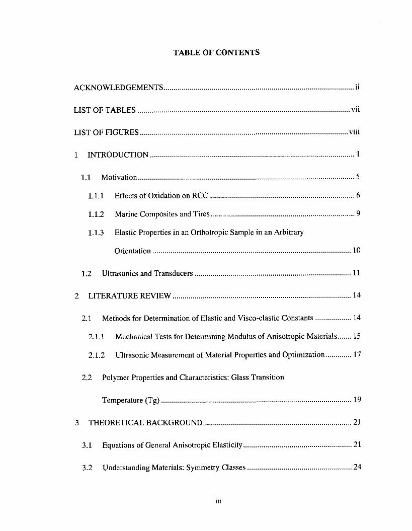
TABLE OF CONTENTS

ACKNOWLEDGEMENTS ............................................................................................... ii

. . LIST OF TABLES .......................................................................................................... vii

... LIST OF FIGURES .................................................................................................. viii

1 INTRODUCTION ...................................................................................................... 1

1.1 Motivation ............................................................................................................ 5

1.1.1 Effects of Oxidation on RCC ........................................................................ 6

1.1.2 Marine Composites and Tires ........................................................................ 9

1.1.3 Elastic Properties in an Orthotropic Sample in an Arbitrary

Orientation ................................................................................................... 10

.............................................................................. 1.2 Ultrasonics and Transducers 11

......................................................................................... 2 LITERATURE REVIEW 14

2.1 Methods for Determination of Elastic and Visco-elastic Constants .................. 14

....... 2.1.1 Mechanical Tests for Determining Modulus of Anisotropic Materials 15

............. 2.1.2 Ultrasonic Measurement of Material Properties and Optimization 17

2.2 Polymer Properties and Characteristics: Glass Transition

Temperature (Tg) ............................................................................................... 19

.......................................................................... 3 THEORETICAL BACKGROUND 21

3.1 Equations of General Anisotropic Elasticity ...................................................... 21

3.2 Understanding Materials: Symmetry Classes .................................................... 24

....................................................................................................... 3.2.1 Triclinic 24

. . 3.2.2 Monoclinic .................................................................................................. 25

3.2.3 Orthotropic ................................................................................................... 26

3.3 Waves in Anisotropic Solids .............................................................................. 27

........................ 3.3.1 Wave Velocity Measurement using Immersion Technique 29

........... 3.3.2 Relationship Between Stiffness Tensor and Engineering Constants 31

3.3.3 Determination of Normals to the Symmetry Planes and Principal

Coordinate System ....................................................................................... 33

3.4 Linear Viscoelasticity ......................................................................................... 37

4 EXPERIMENTAL SYSTEM .................................................................................. 44

4.1 Experimental Setup ............................................................................................ 44

4.1.1 Ultrasonic Immersion Setup for Velocity Data Determination ................... 44

4.1.2 Pulser. Pre-Amplifier and Oscilloscope ...................................................... 45

4.1.3 Experimental Setup for Determining the Initial Guess for Stiffness

.......................................................................................................... Tensor 47

4.1.4 Experimental Setup for Determining the Effects of Oxidation on

Attenuation ................................................................................................... 49

4.2 Experimental Preparations and Procedures ........................................................ 50

4.2.1 Elastic Modulus and Attenuation Determination ........................................ 51

4.2.2 Determination of Effects of Oxidation on Attenuation ............................... 52

4.2.3 Experimental Determination of the Initial Guess Used in Stiffness

Matrix Algorithm ......................................................................................... 52

5 SIGNAL PROCESSING .......................................................................................... 54

.................................................................................. 5.2 Attenuation Measurement 56

.................................................................................. 5.3 Constrained Optimization 61

................................................................................................................. 6 RESULTS 64

6.1 Results for Recovered Elastic Stiffness Tensor and Principal

............................................................................................. Coordinate System 64

6.1.1 Results for RCC ........................................................................................... 64

6.1.2 Results for e-glass Vinylester ...................................................................... 66

6.2 Results for Damping Characteristics ................................................................. 67

6.2.1 Results for RCC ........................................................................................... 68

6.2.2 Results for e-glass Vinylester ...................................................................... 70

6.3 Effect of Oxidation on Damping ........................................................................ 72

7 DISCUSSIONS. CONCLUSION AND FUTURE WORK ..................................... 73

7.1 Stiffness Tensor recovered for RCC .................................................................. 73

............................................. 7.2 Stiffness Tensor recovered for e-glass Vinylester 74

7.3 Damping Measurements and Oxidation Effects ................................................ 74

7.4 Future Work ....................................................................................................... 75

REFERENCES ................................................................................................................ 76

APPENDICES ................................................................................................................. 82

Appendix A . MatLab Routines .................................................................................. 82

Appendix B . More Results and Smoothened Damping Curves .................................. 88

BIOGRAPHY OF THE AUTHOR ................................................................................. 96

LIST OF TABLES

....................................... Table A.l Sample data file recorded using the oscilloscope 87

................. Table B.l Raw data for Figure 6.5. attenuation changes during oxidation 95

vii

LIST OF FIGURES

Figure 1.1

Figure 1.2

Figure 1.3

Figure 1.4

Figure 1.5

Figure 3.1

Figure 3.2

Figure 3.3

Figure 3.4

Figure 3.5

Figure 3.6

Figure 3.7

Figure 3.8

Figure 3.9

3-directional orthogonal weaving [Gauthier. 19951 ..................................... 6

........................................ 3-directional orthogonal weave [Gauthier. 19951 7

Representative RCC sample used in oxidation testing ................................ 7

Results from the initial runs. effects of oxidation on RCC .......................... 9

A sketch of the components of an ultrasonic transducer

[Hellier. 20011 ........................................................................................... 12

Relation between axes and angles in conventional unit cell ...................... 24

An illustration of 3D space lattices and some crystal symmetry

systems . (a) triclinic (a+pq+90°); (b) monoclinic

(primitive. a=y=9007 p+90°); (c) orthorhombic ( a = ~ = ~ = 9 0 ~ ) .................... 26

Ultrasonic wave velocity measurement (a) through reference media

............................................. (b) through anisotropic sample [Auld. 19901 30

Illustration of Euler's angles x" represents the rotated axes ..................... 35

Simplified one-dimensional viscoelastic models .................................. 38

Three parameter viscous model ................................................................. 39

................................................................................ Four parameter model 39

.................................................... Applied stress and response of a sample 41

........................................ Graphical relationship between^'. E' and E" 41

viii

Figure 4.1

Figure 4.2

Figure 4.3

Figure 4.4

Figure 4.5

Figure 5.1

Figure 5.2

Figure 6.1

Experimental Setup .................................................................................... 44

Photograph of experimental setup .............................................................. 45

Longitudinal contact transducers coupled to the sample ........................... 47

Shear contact transducers coupled to the sample ....................................... 48

Photograph of the furnace with cross sectional details .............................. 49

Immersion testing geometry [Schmerr. 19981 ........................................ 57

Attenuation coefficient as measured for an aluminum block and

the best fit straight line for values in the bandwidth of the

transducer (approximately 6-10 MHz) [Schmerr. 19981 ............................ 60

Damping characteristics of RCC. 2. direction for 3 specimens cut

from the same sample ................................................................................. 68

Figure 6.2 Repeatability of damping characterization of RCC. using the same

sample in 4 different tests on different days under same conditions

and same orientation .................................................................................. 69

Figure 6.3 Damping characteristics of e-glass vinylester. 2. direction70 .................. 70

Figure 6.4 Repeatability of damping characterization process of e-glass

vinylester. over 3 different runs on 3 different days under same

conditions and same orientation ................................................................. 71

Figure 6.5 Attenuation changes during oxidation ....................................................... 72

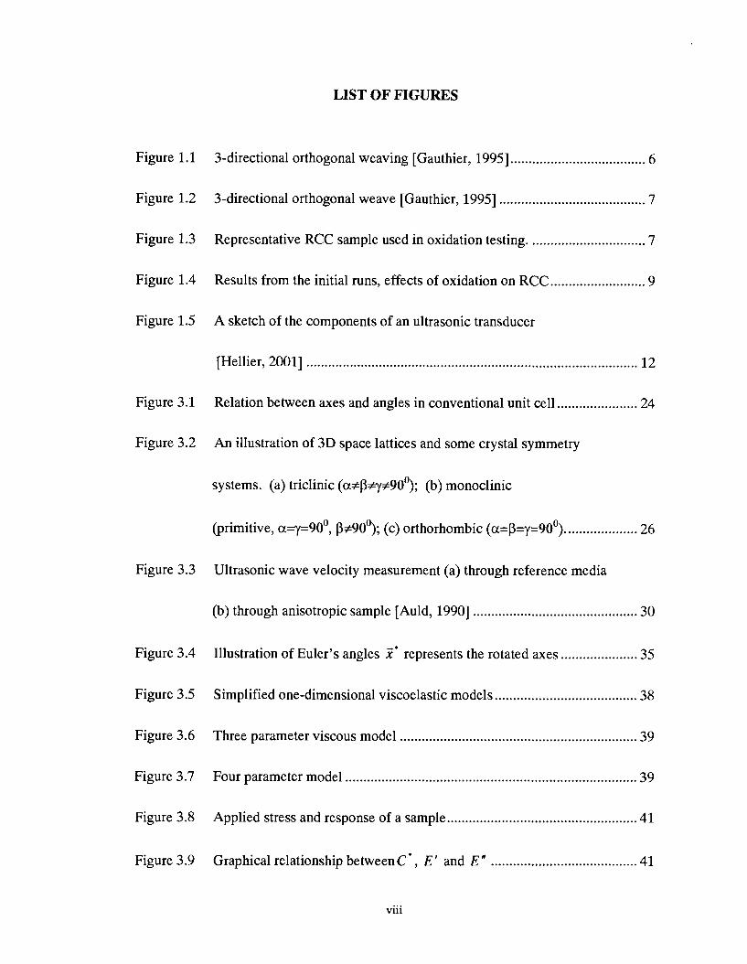
Figure 7.1 Orientation of the e-glass vinylester sample with respect to

. . principal axis ............................................................................................. 74

Figure B.l Damping characteristics of RCC, x, direction, smoothened curve .......... 91

Figure B.2 Smoothened curve showing repeatability of damping

characterization process, over 4 different runs on 4 different days

under same conditions and same orientation for RCC .............................. 92

Figure B.3 Smoothened curve of damping characteristics of e-glass vinylester

in x, direction ............................................................................................ 93

Figure B.4 Smoothened curve showing repeatability of damping

characterization process, over 3 different runs on 3 different days

under same conditions and same orientation for e-glass vinylester .......... 94

1 INTRODUCTION

In order to evaluate the condition of a composite material, elastic properties are

rarely sufficient. In particular, for polymeric material, damping related measurements in

the material provides information about the degree of cross-linking and crystallinity of

the polymer [Menard, 19991. For metals, damping may be related to dislocation motion

among other characteristics. For composite materials, in general the interphase and the

matrix dominate the damping of the material. In particular, for polymer matrix

materials, the fibers are typically very low damping, and the matrix creates damping

characteristics that are anisotropic to the same degree as the elastic constants. For

matrix materials other than polymers, the same may be true depending on the relative

damping characteristic of the matrix and the fibers. This thesis considers damping

characteristics of polymer matrix composites as well as reinforced carbon-carbon

(RCC).

These characteristics represent perhaps the best hope of developing a true index

of state or damage tensor for composite materials. For polymer matrix composites the

combined damping and elastic properties can be combined with either temperature or

pressure to characterize the interatomic potentials in the matrix. This is the closest to a

non-destructive measure of strength that is likely. By describing cross linkage and

crystallinity this measure also provides insight into many of the most important

degradation mechanisms. While a number of failure mechanisms are important in

polymer matrix composites including oxidation and thermal degradation, oxidation

processes generally dominate concern in RCC. The most likely result of the oxidation in

RCC, is a significant change in the damping characteristics of the material [Birman and

Byrd, 20001. This is particularly true in materials where matrix properties may differ

significantly in the region of the fiber (the interphase). The interphase in some materials

is quite distinct, being formed by chemical vapor deposition instead of resin infusion and

carbonization. The diffusion of oxygen into the matrix will tend to occur preferentially

along paths with reduced density, which also makes sample orientation critical. Various

other authors have discussed the importance of damping in evaluating the condition of

other high temperature composites including a review article by Birman and Byrd

[2000]. In general though, it is important to develop a method that is sensitive to the

characteristics of the composite material that are likely to lead to failure. In RCC that

characteristic is oxidation. In polymer matrix composites it is likely changes in

polymerization or oxidative degradation.

The approach is distinct from a perspective taken too often by the non-

destructive testing (NDT) community. In the development of new NDT methods, often

a technique is developed by measurement specialists and applied to a wide range of

problems to determine where the technique is most effective in finding characteristics of

interest. For example, delamination of composite materials and other polymers has been

detected by microwave [Summerscales, 19901, shearography [Newman, 19961,

ultrasonics [Krautkramer, 19751, laser ultrasonics [Anastasi et al., 19981 and

thermography [Zweschper et al., 20031. As a result, there are a number of methods of

finding certain types of defects in composites. Many of these methods continue to be

suspect, however because of other influences such as moisture, conductivity of

reinforcement and inconsistent matrix properties. Alternatively, if the mechanisms of

failure of a material are investigated, then from that basis a method can be found which

is sensitive to the most important failure mechanism. The mechanism should not only

exist in a failed part, but ideally should be shown to be a sufficiently early precursor to

failure to increase reliability. In RCC identification of the mode is reasonably

straightforward, since oxidation of the matrix is the most likely failure mode that is

encountered in high temperature applications. It remains however to be shown that any

method exists which would have sufficient sensitivity to increased reliability. For other

materials, based on environmental conditions, the mechanisms of failure are more

variable and would need to be understood in the context of system reliability.

For reliability of structures, distributed cracking is hypothesized as a precursor to

failure in the mechanics literature. Thus, the detection of cracks has been a key effort in

nondestructive testing. However, even for cracks that are below the critical crack

length, the initiation phase represents a significant portion, if not the majority, of the life

of the component. Thus, mechanisms associated with crack initiation are of great

interest. For composite materials, the initiation failure and initiation phase is typically

associated with the matrix of the material. While the process in polymer matrix

composites is less straightforward, similar effects may be observed when compared to

the material loss mechanisms during oxidation of RCC materials. While the loss of

materials in RCC occurs preferentially in the direction of lowest density portions of the

matrix, similar diffusion related processes occur in polymer matrix composites that can

result in loss of plasticisers or other chemical changes in the matrix. In general, these

mechanisms are oxidative or relate to changes in the degree of polymerization. In high

strain applications, for elastomeric composites, heat generated by the deformation may

also create regions of localized cross-linking or oxidation. Any of these processes, loss

of plasticization, increase in cross-link density, or matrix oxidation will tend to alter the

damping characteristics of the matrix. The changes in the damping will occur primarily

along the geometric axes where the material properties are dominated by the matrix.

However, the geometry of the part can also influence the directions in which the

damping changes occur, since part surfaces where a greater percentage of the area is

dominated by matrix properties will increase the rate of diffusion. Thus, in general, it is

hypothesized that matrix damping may be an effective means of evaluating the condition

of composite materials.

In order to understand the damping in these anisotropic materials, verification of

the principal material axes in composite samples will first be considered. This measure

is required to understand preferred diffusion paths as well as which axis will have high

and low damping. After the material axes are determined for a particular specimen, then

the damping of the material will be determined in the material principal axes for both

dense and oxidized RCC specimens. Similar data for a polymer matrix composite,

which is important for marine composites and wood mechanics, is also considered.

This thesis considers this question: The literature suggests that matrix damping

of composite materials is an important characteristic for evaluation of the condition of a

composite material. Numerous methods exist that allow a damping based "index of

state" to be determined for small samples cut from a composite part. However almost

without exception these methods are only reactive. This investigation explores the

accuracy and repeatability of an ultrasonic method as an absolute measure of material

damping. As part of the measurement of damping in an anisotropic material, it is

necessary to ensure that measurements are made along principal material axis. Thus a

portion of this work is directed toward ensuring that the sample orientation is optimal.

Optimal sample orientation requires recovery of all 21 elastic constants and calculation

of the material planes of symmetry. The damping measures are then made in known

axes of the material.

1.1 Motivation

Mechanical testing methods present perhaps the most well established methods

for obtaining the elastic and damping properties of a material. In addition, mechanical

testing is the only practical method of obtaining strength information on materials. The

scale of the specimens is dependent on a number of issues associated with the acceptable

length scales of materials and edge effects in the sample preparation methods. Using

modern three or four point bend fixtures it is possible to obtain visco-elastic properties

as well as strength properties for small (less than 60 mm long) beams cut from

composite materials. In addition it is possible with mechanical testing to perform the

tests at elevated temperatures. For example Kimura and co-workers [I9821 found the

change in modulus with temperature of a RCC 3mm x 10mm x 60mm long sample using

a four point bending specimen. Dynamic mechanical thermal analysis is similarly used

in polymer matrix composites. For example, damping was used as a damage variable

for water absorption in vinyl-ester glass using 80mm x 13mm x 3mm samples in one

study [Fraga et al., 20031. Young's modulus of a sample was measured from the stress-

strain relations recorded from the experiment and compared to another sample evaluated

at a higher temperature. While static testing of larger samples in mechanical fixtures is

possible, larger specimens create significant cost and complexity even to develop the

basic elastic properties of an anisotropic sample [Bunker, 20021. In addition, some shear

modulus terms are difficult to obtain or are highly uncertain. Non-destructive testing on

small samples to obtain the full properties of a composite would be an ideal way of

determining the mechanical properties, as well as making it possible to use these

measurements in quality control or inspection application.

1.1.1 Effects of Oxidation on RCC

To understand the effects of oxidation on RCC an understanding of the structure

of the material is necessary. RCC composites are materials that consist of carbon fibers

embedded in a carbonaceous matrix. The particular carbon composite used in this work

is composed of a 3-directional, orthogonal, carbon fiber weave. The general

configuration is illustrated in Figure 1.1 and Figure 1.2 [Gauthier, 19951. Figure 1.3

shows an example of the sample used in this thesis

Figure 1.1 3-directional orthogonal weaving [Gauthier, 19951

6

Figure 1.2 3-directional orthogonal weave [Gauthier, 19951

Figure 1.3 Representative RCC sample used in oxidation testing.

RCC is an useful material because of its increased strength at elevated

temperatures [Savage, 19931. One major limitation to the application of RCC

composites for high temperatures is the susceptibility to oxidation. Carbon composites

readily react with oxygen at temperatures as low as 400°C. This reaction results in loss

of material (primarily the matrix) and a degradation of the mechanical properties of the

material. Both the strength and the modulus of the material are likely to change as

structural material is lost. Consequently, protective coatings are often deposited on the

RCC composite in order to prevent this reaction from occurring in high temperature

environments. In use these protective coatings can crack and expose the material to an

oxidizing environment. This can lead to localized oxidation of the material, which also

creates stress concentrations in the part. This is the mechanism, which appears to have

led to the loss of the NASA orbiter Columbia [Gehrnan, et al., 20031.

A continuing need thus exists to perform experiments to better understand the

oxidation process and to understand how to measure oxidation in RCC. Currently, no

in-situ method exists to study the effects on mechanical properties of oxidation of RCC

composites. During oxidation, matrix degradation occurs and thus the damping would

be expected to change. Initial results were obtained from a trial run of oxidizing RCC

samples. Seven RCC samples were heated to 700°C and were oxidized to different

levels (to get different weight loss). Figure 1.4 shows a plot of attenuation vs weight

loss.

I I I I I I I

4 5 6 7 8 9 10 Weight loss (Oh)

Figure 1.4 Results from the initial runs, effects of oxidation on RCC

In Figure 1.4, a distinct pattern emerges for the behavior of RCC during oxidation. As

the weight loss increases the attenuation increases. Most importantly, the changes are

quite large at lower weight losses. Other methods are less likely to detect oxidation but

show that significant reductions in material strength may occur.

1.1.2 Marine Composites and Tires

Additional applications of the same techniques are possible if sufficient accuracy

is obtained. In particular, polymer matrix composites are used extensively and are well

suited for marine applications. Inspection is needed to detect manufacturing defects,

such as incomplete catalyzation of the resin, or excess catalyst that serves as a

plasticizer. Similarly tires are susceptible to heat related changes in the elastomeric

matrix. These changes are most likely to be detected using measurements of material

damping. However, like polymeric composites, the changes are expected to be modest.

In both systems, layered media needs to be characterized accurately to separate subtle

damping changes in a layer. The accuracy and the repeatability of the measurements are

critical.

1.1.3 Elastic Properties in an Orthotropic Sample in an Arbitrary Orientation

The first portion of this thesis considers the recovery of elastic properties of a

general anisotropic material. Earlier work considered the determination of elastic

constants of single crystal materials and RCC using a large number of ultrasonic

measurements and optimization [Sun, 20021. This work was incomplete because of

problems with not satisfying constraints in the relationship between the constants.

While RCC is nominally orthotropic material with 3 orthogonal planes of symmetry, the

manufacturing method suggests that the symmetry may be lower. As such it is assumed

that 21 independent variables are required in the constitutive relationship, the most

general case of an anisotropic material.

The RCC is not assumed to be orthotropic because of the process used to

produce the material. RCC is produced from a 3-dimensional preform, which is

nominally orthotropic (3 planes of symmetry). However in RCC, the matrix is

introduced into the interstices in the fiber preform using either chemical vapor infusion,

resin infusion or a combination of vapor infusion and resin infusion. If resin infusion is

used, multiple infusions are used with carbonization of the resin after each infusion.

This leads to a diffusion density gradient that may differ in geometry from the matrix

preform. Thus while it is tempting to assume that the finished composite retains the

symmetry of the fiber preform, nothing in the material manufacturing process ensures

that this is in fact the case. Significant variations of these planes can also exist due to

fiber misorientation. The earlier work also considered methods to recover the planes of

symmetry from experimental data sets. These data sets are not necessarily oriented in

the planes of symmetry and thus may produce a fully populated compliance tensor even

in the absence of reduced material symmetry. The ultrasonic technique involved the

determination of the compliance tensor in an arbitrary orientation and then defining the

orientation. The prior work was effective at implementing the orientation techniques

however the optimization algorithms used were suspect because of the instability of the

results and not satisfying constraints on compliance explicitly. This thesis extends the

optimization procedure and explores methods to improve stability.

1.2 Ultrasonics and Transducers

Ultrasonic waves represent propagating regions of densification and rarefication

of an elastic media. By definition ultrasonic waves have frequencies that are too high to

be detected by the human ear. While a typical human being can hear sound in the range

of 2 Hz to 20 KHz, typical ultrasonic frequencies range from 100 KHz to 80 MHz. In

this work 1MHz central frequency transducers are used. This results in a wavelength of

approximately 5mm in the material used.

Both generation and detection of ultrasound is typically done using a

piezoelectric transducer. The transducer transmits the mechanical energy into the

sample. A sketch of an ultrasonic transducer and its components is shown in Figure 1.5

Figure 1.5 A sketch of the components of an ultrasonic transducer [Hellier, 20011

Three main components of an ultrasonic transducer are the piezoelectric or active

element, backing, and an impedance matching plate. The piezoelectric element is

capable of both receiving and generating elastic waves, the piezoelectric effect and the

inverse piezoelectric effect, respectively. The backing is a highly dense material that

controls the propagation of other vibration modes of the transducer by absorbing the

energy radiating from the back face of the active element and thus shaping the pulse.

Depending on the way the element of the transducer is cut, either shear or

longitudinal waves can be generated. For transmission of the signal into water, shear

transducers are not used since the shear wave cannot propagate in liquid medium.

However, both shear and longitudinal transducers are used in contact applications where

the wave is directly transmitted into a solid material without an intermediate fluid

coupling. Immersion transducers are used in most of the experimental work in this

thesis because of the ability to continuously change the angle of the incident wave onto

the sample. The range of incident angle is also used to generate both longitudinal and

shear waves in the sample as a result of mode conversion at the water interface

[Achenbach, 19841. This provides the large number of signals required to perform the

over constrained optimization used to recover the elastic constants.

2 LITERATURE REVIEW

2.1 Methods for Determination of Elastic and Visco-elastic Constants

A number of methods are used to measure the elastic and viscoelastic constants

of materials. These are based on either the static or dynamic response of the material to

an applied excitation [Schreiber et al., 19731. The most common method for the

determination of the elastic constants was static testing, such as tensile, compressive,

and torsional tests [Every and Saches, 19901. Most of the methods are quite

straightforward when applied to homogeneous isotropic solids. For an isotropic material

only two independent constants exist. So a simple tensile test can be combined with a

torsion test to obtain the elastic constants. Dynamic or creep tests are then used to

obtain material damping. Damping measurements must be performed at a range of

frequencies since material damping is in general, frequency dependent. Absolute

measurement of material damping is challenging because of the dependence on

boundary conditions.

In anisotropic materials that are characterized by additional independent elastic

constants, mechanical testing is more difficult. In anisotropic materials a number of

samples cut at different orientations must be measured. These samples must be

representative of the material even though they are cut from different locations. As a

result of the testing needs, dynamic methods have been developed. The dynamic

methods include ultrasonic transmission [Chimenti, 19971 and resonance method

[Migliori and Sarrao, 19971. Dynamic methods also allow viscoelastic properties to be

obtained and can be used to probe some material non-linearities. Most importantly,

dynamic methods can recover all of the elastic constants from a single sample, which

reduces the uncertainty in the results. The most widely used methods are, or have been

adapted from [Hellwege, 19791

Bulk acoustic and ultrasonic wave techniques, including the ultrasonic wave

transmission and pulse superposition methods.

Resonance samples in the shape of rods, bars, parallelepipeds, plates, and

more recently spheres.

Static deformation.

Light, neutron, and X-ray scattering, including Brillouin Scattering.

In general, the accuracy of the methods differs widely with the list above. The

technique of ultrasonic transmission and Brillouin scattering are the most commonly

used methods. Brillouin scattering allows the measurements to be made on samples that

are a few millimeters in size. Brillouin scattering cannot provide information about the

effect of temperature on the elastic constants. In general, ultrasonic transmission

methods hold significant advantages if a full set of elastic constants is required

[Hellwege, 19791.

2.1.1 Mechanical Tests for Determining Modulus of Anisotropic Materials

During the 1980's, a number of mechanical test methods were introduced along

with the development of new composite materials. The development of many new

composite materials led to these innovations. Some of the new composite materials

included those incorporating toughened epoxy, bismaleimide, polyamide, and high

temperature thermoplastic matrix materials, pitch-precursor carbon fibers, and

polyethylene and other organic fibers. The new test methods provided a means of

discriminating between the new material systems becoming available. The most

common mechanical test configurations were tensile, compressive, shear and flexure.

All of these testing methods can be used to obtain both elastic constants and to measure

the ultimate strength of the material [Jenkins, 19981.

ASTM D 3039, ASTM D 5467 and ASTM D 2344 illustrate some of the most

commonly used tensile, compressive and shear tests for composites [Jenkins, 19981. All

of these tests follow the general rule, apply load, measure strain and find modulus as a

ratio of stress over strain. These tests are very specific on how the sample is prepared

and on the procedure itself. For characterizing a composite, or any other kind of

anisotropic material, these tests require samples to prepared for each orientation. This

makes the sample preparation cumbersome. Another major drawback of these tests is

the testing environment. The testing environment can affect the repeatability and

accuracy of the results [Menard, 19991. Most of the standard tests are for large samples,

i.e., samples whose lengths vary from 5 cm to meters long and width anywhere between

1 cm to meters wide. Most of these tests are conducted at the ambient condition of the

lab where the test is being conducted, since controlling of the test condition is very

difficult with large samples.

A solution to controlled testing is dynamic mechanical thermal analysis

(DMTA), also referred to as dynamic mechanical analysis (DMA). DMA is an

experimental technique which analyzes the material's response to an applied dynamic

excitation under controlled conditions [Menard, 19991. DMA achieves this by analyzing

small samples. Samples generally are not longer than 4 cm and not more than 5 mm

thick. DMA is a widely accepted research technique in the polymer industry for the

determination of material's properties such as viscosity, modulus and damping,

providing important information about curing of thermoset resins and the aging of

thermoplastics [Menard, 19991. Even though DMA solves the problem of controlled

testing, the number of samples required to characterize a composite is still large.

2.1.2 Ultrasonic Measurement of Material Properties and Optimization

The technique of using ultrasonic transmission to characterize material properties

has developed significantly over the past fifteen to twenty years [Chimenti, 19971.

There are many references focusing on methods for obtaining the elastic constants using

the ultrasonic technique [Jenkins, 19981. Chimenti [I9971 provides an overall review of

the various methods available. In ultrasonic transmission approaches, the specimen is

either immersed in a fluid or in direct contact with the transducer. A limitation of the

direct contact technique is that it usually requires a fairly thick sample (3 to 5 cm), and it

also requires cutting the testing sample at different angles as in mechanical methods

[Rokhiin and Wang, 1992; Baudouin and Hosten, 19971. In the past, one important

drawback of the immersion technique, especially for in-service inspections, was the need

to immerse the material in a liquid, usually water or oil. However, modern transducer

technology has allowed significant reduction in signal noise and air-coupled ultrasonics

is now successfully applied for the viscoelastic characterization of composite materials

[Hosten, 19911. Many studies have shown that immersion methods are more

straightforward to apply and usually give better results [Papadakis et al., 1991; Hosten,

19911. Another major advantage over the mechanical testing methods is the reduction in

number of samples required to characterize a material. Using one single sample a

material can be characterized completely. However, significant complexity is

introduced due to the need to perform constrained optimization to measure the sample

[Aristegui and Baste, 19971.

Identification of elastic constants from the measurement of wave velocity using

ultrasonic techniques involves evaluating Christoffel's equation [Aristegui and Baste,

19971. Two major approaches have been applied to find the solution of the Christoffel's

equation, numerical techniques [Aristegui and Baste., 1997; Chu et al., 19941 and direct

solution expressed in a closed form [Rokhlin and Wang, 19921. A numerical technique,

non-linear optimization, is used in this thesis.

The elastic constants can be reconstructed from the amplitude and velocity data

by performing a Newton-Raphson nonlinear optimization to the experimental data.

Christoffel's equation is the pivotal equation to be solved to get the required numbers

[Aristegui and Baste, 19971. Christoffel's equation is a cubic equation and applies to

plane waves in both isotropic and anisotropic media. The optimization to be performed

here is a constrained optimization since the compliance must be positive definite. The

format of constrained optimization requires the function to be compared to some

limiting value that is established by the constraints [Venkataraman, 20021. In a

constrained optimization problem meeting the constraints is more paramount than

optimization. All the numerical techniques used for solving the Christoffel's equation

follow the above stated basic rules [Aristegui and Baste, 1997; Chu et al., 19941. In

general velocity data obtained from ultrasonic techniques is subjected to a nonlinear

least squared optimization with inequality constraints. Detailed explanation of

Christoffel's equation and mathematical derivation to get the stiffness tensor from the

Christoffel's equation is included in chapters 3 and 5.

2.2 Polymer Properties and Characteristics: Glass Transition Temperature (Tg)

In order to apply these damping measures to understand the degradation of

polymer matrix composites it is helpful to review some basic polymer material

properties. The glass transition (Tg) is probably the most fundamental characteristic of a

polymer. Among the thermal transitions and relaxations observed in amorphous

polymers it is certainly the most important. When an amorphous polymer undergoes the

glass transition, almost all of its properties that relate to its processing and/or

performance change dramatically. The coefficient of thermal expansion increases from

its value for the glassy polymer to a much larger value for the rubbery polymer when the

temperature increases to above the Tg. During the transition mechanical properties

undergo significant changes as well, the viscosity above Tg is lower than the viscosity

below Tg by many orders of magnitude [Bicerano, 19931. The mechanical experiments

clearly demonstrate that the transition from the glassy to the liquid state is purely

kinetical phenomenon. Whether the compliance of a sample is small as in a glass, or

large as for a rubber, it depends only on the measuring time or the applied frequency.

Rubber elasticity originates from the activity of 'a-modes', a major group of relaxation

processes in polymer fluids [Strobl, 19961.

The glass transition plays an important role in determining the physical

properties of semi-crystalline polymers, whose amorphous portions "melt" or "soften" at

Tg while the crystalline portions remain "solid" up to the melting temperature (Tm). A

semi-crystalline polymer can be treated as a solid below Tg, as a composite consisting of

solid and rubbery phases of the same chemical composition between Tg and Tm, and as

a fluid above Tm. The effect of glass transition on physical properties of semi-

crystalline polymers decreases with increasing crystallinity [Bicerano, 19931. In the

context of this thesis the thermal transitions are important because it is widely used in

various polymeric systems to describe the degree of crystallinity and cross-link density

in a material. In the vicinity of Tg, the modulus typically varies from the glassy

modulus (ca. lo9 Pa) to the rubbery modulus (ca. lo6 Pa). The general interpretation for

the glass transition is "freezing of molecular motions", i.e. competition between the

molecular relaxation time scale and experimental time scale.

3 THEORETICAL BACKGROUND

The measurement of elastic properties using ultrasonic waves is dependent on the

relationship between modulus and ultrasonic wave velocity. These concepts are

important in understanding the results of the measured wave speed. In addition, the

reaction between symmetry planes and elastic constants is an important aspect of these

measures in anisotropic materials. Finally the relation between the measures of

ultrasonic wave attenuation and damping are discussed.

3.1 Equations of General Anisotropic Elasticity

For this application the infinitesimal strain tensor, E+ describes the deformation

in an acoustical excitation of a body. The strain is related to the particle displacement

field u,, through the stress-displacement equation [Fung, 20011

where ui, and u j,i are the first partial derivative of displacement with respect to the

coordinate index jand i , respectively. In the following discussion a summation

convention will be observed.

From dynamics, the elastic restoring forces are defined in terms of stress field oi,.

The equation of motion in a freely vibrating body is [Fung, 20011

0.. . = pui 1 1 9 I

where oij*, is the partial derivative of stress with respect to the coordinate index j . The

superposed double dots, iii indicates the second partial derivative of displacement with

respect to time.

The constitutive equation, Hooke's law, states that the stress is linearly

proportional to strain as well as the converse [Auld, 19901.

Oij = Ci jk lEk l

The elements of the tensor Cijkl in equation 3.3 are called elastic constants.

Since there are nine equations in equation 3.3 (corresponding to all

combinations of the subscripts ij ) and each contains nine strain terms, Cijkl has indeed a

total of 81 components. However, they all are not independent. The symmetry

properties of the stress and strain

0. . = 0 . . , & 11 11 kl = Elk

indicate

Cijkl = C jikl = Cijlk = C jilk 3.5

Thus, the independent components of Cijkl are reduced from 81 to 36. If Poynting's

theorem is applied, it can be shown that

= C,,

The number of independent constants are then further reduced to 21. This is the

maximum number of independent elastic constants for any material symmetry. If the

symmetry properties imposed by the microscopic nature of the material are considered,

the number is typically less than 21. The number of independent constants has range

from 2 (isotropic) to 21 (triclinic).

The four subscripts of Cijk, can be simplified to two subscripts by using the

following abbreviated subscript notation [Fung, 20011:

It can be shown that formally this relates a 3 dimensional 4th order tensor to a 6

dimensional 2nd order tensor if proper normalization is used [Norris, 19881.

The compliance tensor C is written as a 6x6 symmetric matrix form

-

'11 '12 '13 '14 '15 '16

'22 '23 '24 '25 '26

'33 '34 '35 '36

c, c 4 5 c, ~ y m . C55 C56

'66. -

or in tensor notation as

C T p = C W ~ q

in this section the normalization will not be used, so matrix terminology is followed.

3.2 Understanding Materials: Symmetry Classes

Using the framework of compliance, symmetry of anisotropic materials can be

described. In three dimensions, the 32 symmetric point groups can be subdivided into

14 space lattices. These lattices are further grouped into seven crystal systems: triclinic,

monoclinic, orthorhombic, tetragonal, cubic, trigonal, and hexagonal [Musgrave, 19701.

The first three symmetry classes (triclinic, monoclinic, and orthorhombic) are

considered to be the lower symmetry systems than elastic bodies typically exhibit. The

remaining are considered to be the higher systems [Fedorov, 19861. The derivation of

the symmetry groups can be found in various textbooks. Figure 3.1 describes the

relation between the axes and the angles of the unit cells in an anisotropic media. Some

lower symmetry systems are given here to show how the symmetry properties reduce the

number of independent elastic constants.

Figure 3.1 Relation between axes and angles in conventional unit cell

3.2.1 Triclinic

Triclinic is the absence of any material symmetry in the solid. There are no

relationships between the 21 elastic constants, and none are zero. Figure 3.2 (a) shows

3D space lattices in a triclinic crystal and the corresponding symmetry system. The

angles a , P , y are not equal and none of the angles are equal to 90' [Musgrave, 19701.

This result implies that no planes of symmetry exist in this system or any rotational

symmetry.

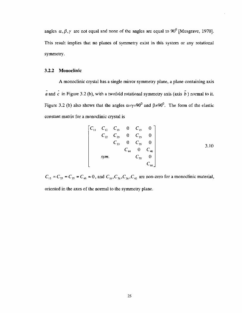
3.2.2 Monoclinic

A monoclinic crystal has a single mirror symmetry plane, a plane containing axis

- o and c in Figure 3.2 (b), with a twofold rotational symmetry axis (axis ) normal to it.

Figure 3.2 (b) also shows that the angles c~=~=90' and p+90°. The form of the elastic

constant matrix for a monoclinic crystal is

C,, = C,, = C3, = C,, = 0 , and C,, , C,, ,C3, ,C,, are non-zero for a monoclinic material,

oriented in the axes of the normal to the symmetry plane.

(4

Figure 3.2 An illustration of 3D space lattices and some crystal symmetry systems.

(a) triclinic ( a + q # 9 0 ~ ) ; (b) monoclinic (primitive, a=y=90°, ~ $ 9 0 ~ ) ; (c) orthorhombic

(a=~=~=90O).

3.2.3 Orthotropic

Orthotropic, also called orthorhombic symmetry, is characterized by three

mutually perpendicular mirror symmetry planes and twofold rotational symmetry axes

perpendicular to these planes with angles a=y=~=900 as shown in Figure 3.2(c).

Orthorhombic materials have nine independent elastic constants. The elastic constants

for an orthotropic sample which is oriented with the principal axis forming basis for the

coordinates.

' 1 1 '12 '13 O O O

' 2 2 ' 2 3 O O O C3, 0 0 0

C , 0 0

sym. c 5 5 0

C 6 6

Using these three cases it is then possible to discuss the propagation of elastic waves in

anisotropic solids.

3.3 Waves in Anisotropic Solids

From the constitutive equation 3.3 and equations 3.1 and 3.2 we get [Auld, 19901

A plane wave solution to this second order differential equation is assumed to be of the

form [Auld, 19901

[ere A, are compo

C i i k r ~ k , j l = P U i 3.12

uk = ~ ~ ~ ~ e ~ ( ~ ~ - ~ ) 3.13

lnents of the displacement amplitude; p, are unit displacement

polarization vectors traveling in the directions determined by the relationship between

the incident angles and the material symmetry axes; k = * is the wave number with

wave speed in the solid c and frequency o [Auld, 19901. In general the wave speed c is

a function of the elastic compliance of the material and the density of the material.

Substituting equation 3.13 into equation 3.12 gives an eigenvalue equation (Christoffel's

Equation), then,

j n l - 'ik pv2 )P, = O 3.14

This is a cubic polynomial in pV2, where V is the phase velocity of the ultrasonic

wave, 6, is the Kronecker delta symbol, n is a unit vector in the direction of wave

propagation with components of nl,n2,n3. Equation 3.14 can be rewritten in matrix

form [Auld, 19901:

where

is referred to as the Christoffe17s tensor.

Christoffe17s tensor is indeed a second order tensor, subject to the symmetry

condition rik=rki [Hearmon, 19611. Therefore, six independent components of the

Christoffe17s tensor exist. Expansion of equation 3.16 following indicia1 rule gives

In order to have a nontrivial solution of the Chirstoffel's equation, the determinant of the

coefficient matrix of equation 3.15 must vanish.

Since the Christoffel's tensor Ti, is symmetric, its eigenvalues p V 2 are real and

the eigenvectors p, are mutually orthogonal. Therefore, for any given direction n, three

modes can be generated with different velocities and polarizations. For the principal

propagation directions, pure propagation modes can be generated: one longitudinal wave

when P=n, and two transverse waves when Pxn=O. In general, a quasi-longitudinal

wave (QL) and two quasi-transverse waves (QT1 and QT2) are excited. The phase

velocities corresponding to each of these wave modes are known to be functions of the

elastic properties of the material.

3.3.1 Wave Velocity Measurement using Immersion Technique

In the immersion technique the transducers and the sample are immersed in the

water or any other coupling media. Consider a coordinate system R = (2, ,2,,2,) where

R is set at the center of the sample. Unit base vector z;., is normal to the interface, with

the other two following the right hand rule. For a fluid coupling of an ultrasonic wave

into an anisotropic plate, and for an arbitrary incident angle 8, three modes of the wave

are excited. A quasi-longitudinal wave (QL), a slow quasi-transverse wave (QT1) and a

fast quasi-transverse wave (QT2) are generated in the solid as illustrated in Figure 3.3.

These waves propagate at different phase velocities and all the velocity vectors lie in the

incident plane. If this plane coincides with a plane of the material symmetry, only one

transverse wave and one longitudinal wave are generated [Auld, 19901. The second

transverse polarization is not required to satisfy the boundary conditions at the fluid

solid interface.

Transmitting transducer

Transmitting transducer

L r

( 4 €!El Receiving

- transducer

\ 2 Receiving V transducer

Figure 3.3 Ultrasonic wave velocity measurement (a) through reference media (b)

through anisotropic sample [Auld, 19901

To measure the phase velocity, the length of the wave path through the plate

must be known. The relative time delay ri between the transmitted signal through the

sample and the time through a known media must also be obtained. In this case the

known media is the water path without the sample. The time delay is obtained by cross

correlation [Peterson, 19971 and will be explained later in section 5.1. The length of the

wave path is obtained by Snell-Descartes law [Auld, 19901. The velocities then can be

calculated by the formula [Hosten, 20011

where Vo is the wave velocity in water, Ti is the time delay, Bi is the incident angle, d is

the thickness of the sample, and (2 , , cp) indicates the wave incident plane.

In order to identify the full set of elastic constants of a general anisotropic

material, experimental data is collected from four incident planes (Z,, cp), where cp=oO,

45', 90' and 135' are called the azimuthal angles [Aristegui and Baste, 19971.

3.3.2 Relationship Between Stiffness Tensor and Engineering Constants

Engineering constants of an orthotropic material are generalized as Young's

moduli, Poisson's ratios and shear moduli, as well as some other behavioral constants

[Jones, 19751. These constants are measured in simple tests, which are illustrated later is

section 4.2.2.3. The relationship between longitudinal wave speed, cl and shear wave

speed, G, to the engineering constants is given by [Grigoriev and Meilikhov, 19971

2 - 4 G(4G-E) p c , = A + 2 G = K + - G = 3 3G-E

From speeds in all three directions for a material, El, E2, E3, G12, G13 and G23 can be

determined from equations 3.20 and 3.21. El, E2 and E3 are the Young's moduli in 1, 2

and 3 direction respectively, G12, G13 and G23 are shear moduli in 2-3, 1-3 and 1-2 planes

respectively. The components of the compliance matrix can be determined as

where uij is the Poisson's ratio for transverse strain in the j direction when stressed in

the i direction. Since stiffness and compliance matrices are mutually inverse, it follows

by matrix algebra that their components are related as follows for orthotropic materials

where

3.3.3 Determination of Normals to the Symmetry Planes and Principal

Coordinate System

Based on the knowledge of the elastic constants Cijkl of an anisotropic material,

identification of elastic symmetry possessed by the material was developed by Cowin

[1987, 19891 and Norris [1988]. Two tensors, Aij , the Voigt tensor, and Bij ,the

dilatational modulus are required to determine the elastic symmetry planes of the

material. These tensors are defined as

If the abbreviated subscript notation Cij is used and by applying the indicia1

notation, tensors A and B can be expressed in terms of the components of Cij

A vector is normal to a symmetry plane of a linear elastic material, if and only if,

the vector is an eigenvector of tensor A and B respectively. These normals are in a

specific direction and define a specific axis [Cowin, 19891. Once the specific directions

and specific axes are obtained by solving the eigenvector problem of A and B, the elastic

symmetry of the anisotropic material can be determined.

Theoretically, for an orthotropic material, the three eigenvectors of tensor A and

B are coincident and are aligned with their crystallographic directions [Cowin

Mehrabadi, 19871. For a monoclinic media, only one pair of eigenvectors is identical.

In the case where none of the eigenvectors are in common indicates that the material

tested possesses triclinic symmetry. However when using experimental data, errors in

the measurements result in eigenvectors of A and B that do not exactly line up. Since

the eigenvectors of A and B are orthogonal eigenvectors, respectively, a normal to the

symmetry plane is contained in an angle around the average directions between the

closest eigenvectors of A and B [Aristegui and Baste, 20001. The closest eigenvectors

of A and B can be determined by investigating the angular deviation between each pair

of eigenvectors. In general the eigenvector pair that exhibits the small angular deviation

is considered to be a good estimate of a normal to a symmetry plane [Aristegui and

Baste, 20001

Once the normals to the symmetry planes are known, recovery of the principal

coordinate system becomes relevant. In some design applications, knowledge of the

principal coordinate system is necessary to predict the misorientation between the

symmetry axes and the geometric axes within the material. It can also increase the

understanding of the warpage and coupled deformation.

As described in section 3.2, seven symmetrical crystal systems exist. The

number of symmetry planes it possesses and the orientations of these symmetry planes

characterize each system. The orientation of a principal coordinate system, R' with

respect to an observation coordinate system R as defined in section 3.3.1 can be

specified by a set of Euler's angles 6= (a, P, y). Euler's angles relate the two coordinate

systems R' and R through a set of successive rotations between the two systems.

No general agreement on the notation of Euler's angles exists, but one of the

most common, viz. a , P, and y, in sequence, is shown in Figure 3.4. The coordinate

system R with a set of Cartesian axes i, ,i2 and 2, is first rotated through an angle a

about the i, axis. A further rotation through angle P about the transformed 2, brings the

body into a coordinate system R'. Finally a second rotation y about the transformed

- x, put the system into a coordinate system R' with a set of Cartesian axes i,P , 2:' and

2:. The rotations are performed as counterclockwise as one looks to the origin 0 along

the axis of rotation [Shames, 19661. It is also important to note that the orientation of

the rotated coordinate frame is dependent on the order of the rotations.

Figure 3.4 Illustration of Euler's angles 2' represents the rotated axes

Transformations from the initial R to the coordinate system R' may also be obtained

through three-transformation tensors a(a), a@), a(y) .

kip J= [a(a)I[a(P)][a(~ )]{xi I = [ M I B ~ I

where

which can be combined to give

cos@) cost) -sin@) cosf? )sink) sin@) cost) +cos@) cosf?) sink) sin@) sink)

sink) -sin@) cosf?) c o s u -sin@) sink) +cos@) cosf?) cost) sin@) cos t )

sin@) sin@) -cos@) sin@) cosf?) I 3.30

Locating the principal coordinate system RP (if it exists within the material) is equivalent

to the determination of the set of angular unknowns, S=(a, P, y). Each of the angular

unknowns corresponds to a normal to the symmetry plane and transforms the coordinate

system from RP to R. In general, two rotations of the coordinate system are enough to

characterize the orientation of the principal coordinate system RP [Auld, 1990; Aristegui

and Baste, 20001. In other words, any principal coordinate system RP, with respect to

the observation coordinate system R, can be characterized by a set of angular unknowns

with at least one of these unknowns being equal to zero. Therefore the transformation

matrix [MI in Equation 3.30, if y=O as in this thesis, can be reduced to

For the case where the material possesses higher symmetries (tetragonal, hexagonal or

isotropic), the principal coordinate system can be identified, based on the symmetry

model assumed. The orientation of the axes is found by investigating the deviation

between the elastic constants reconstructed in RP and the one satisfying the chosen

symmetry model [Aristegui and Baste, 19971. In the case where the material possesses

only a single symmetry plane, identification of the symmetry is reduced to finding one

unknown of the Euler's angles with the two other angles zero. On the other hand, if no

symmetry can be determined, three Euler angles 6=(a, P, y) are necessary to search for

RP [ Aristegui and Baste, 19971.

3.4 Linear Viscoelasticity

In addition to the elastic properties the damping properties are used in this thesis

to describe the equations of state of the materials. This explanation can be done in terms

of linear viscoelasticity in the principal axis of the material because the elastic properties

have been measured and the sample has been oriented in the principal material axes

prior to measuring damping. Linear viscoelastic behavior is often idealized as a

combination of springs, to represent purely elastic or Hookean behavior, and dashpots to

represent purely viscous or Newtonian behavior.

The one-dimensional problem is suitable for samples oriented in principal axes

as well as being often used as a tool to help understanding linear viscoelastic behavior.

In this case, the combination of elements - spring and dashpot - is arranged in series and

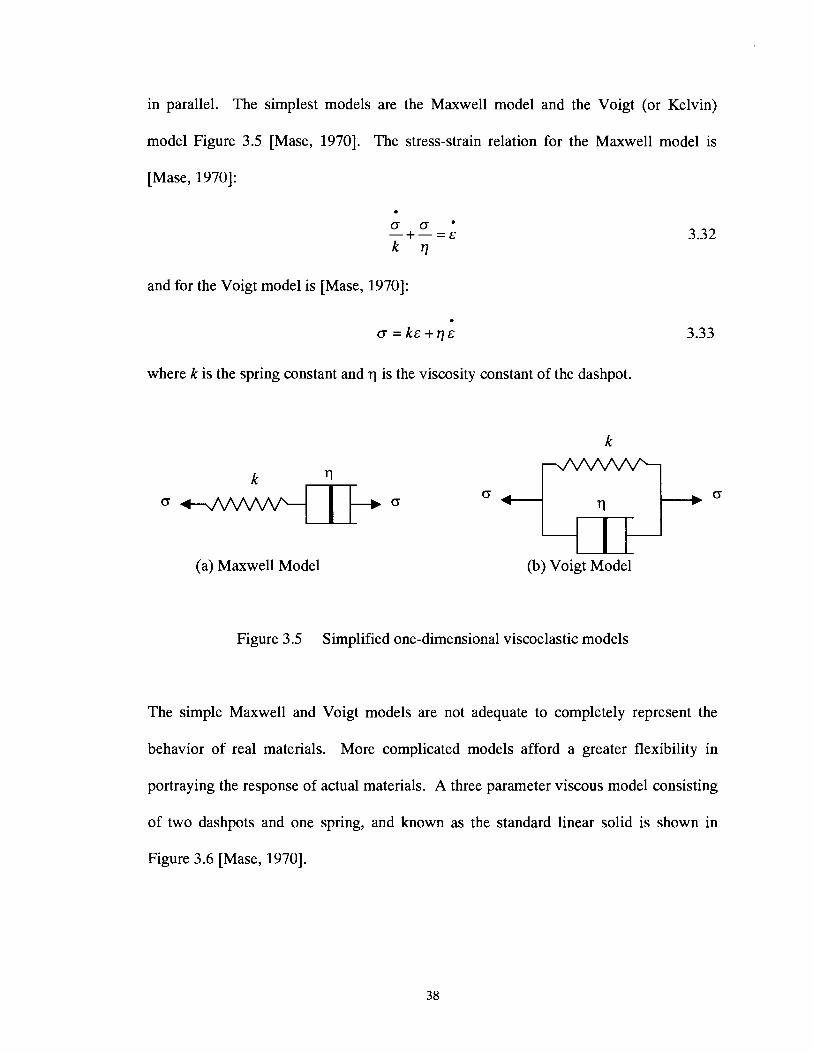
in parallel. The simplest models are the Maxwell model and the Voigt (or Kelvin)

model Figure 3.5 [Mase, 19701. The stress-strain relation for the Maxwell model is

[Mase, 19701:

and for the Voigt model is [Mase, 19701:

where k is the spring constant and -q is the viscosity constant of the dashpot.

(a) Maxwell Model (b) Voigt Model

Figure 3.5 Simplified one-dimensional viscoelastic models

The simple Maxwell and Voigt models are not adequate to completely represent the

behavior of real materials. More complicated models afford a greater flexibility in

portraying the response of actual materials. A three parameter viscous model consisting

of two dashpots and one spring, and known as the standard linear solid is shown in

Figure 3.6 [Mase, 19701.

A four parameter model consisting of two springs and two dashpots may be regarded as

Maxwell unit in series with a Voigt unit as illustrated in Figure 3.7 [Mase, 19701.

(3 4

Figure 3.7 Four parameter model

The four parameter model is capable of all three of the basic viscoelastic

response patterns. Thus it incorporates "instantaneous elastic response" because of the

free spring kl , "viscous flow" because of the free dashpot 771, and, "delayed elastic

response" from the Voigt unit. The stress strain equation for any of the three or four

parameter models is of the general form [Mase, 19701:

Figure 3.6 Three parameter viscous model

772 b 0

p2cY + pld + poo = q2& + q,& + q , ~ 3.34

Where the pi's and qi's are coefficients made up of combinations of the k's and q's and

depend upon the specific arrangement of the elements in the model [Mase, 19701.

Complex modulus notation is used to mathematically represent the characteristic

of a viscoelastic material, by combining damping and stiffness expression [Jenkins,

19981. Another form of the stress strain equation represented by equation 3.34, using

complex modulus notation, is

o( t ) = C*(O) ~ ( t ) 3.35

where

The complex compliance C* is

and the loss factor is

o is the frequency, t the time, E 1 ( o ) and E W ( o ) are the elastic (or storage) modulus

and loss modulus, respectively, and 6 ( 0 ) is the phase angle between the applied stress

and strain. The relationship between these quantities is shown in Figure 3.8 and Figure

3.9. When we apply an oscillating stress to a sample, the response signal will not be

similar to the applied signal. This is due to the various losses attributed to the elastic

and viscous behavior of the sample, the strain lags the applied stress by the phase angle

6 [Menard, 19991.

Applied Phase angle = 6

I Stress I

Time

Material response

Figure 3.8 Applied stress and response of a sample

Elastic modulus (E '(a))

Figure 3.9 Graphical relationship between C * , E ' and E "

The tangent of the phase angle, tan 6, is the ratio of loss modulus to storage

modulus and is a valuable indicator of the material's relative damping ability.

In contrast to many introductory texts on linear viscoelasticity the current interest

is in the measurement of damping effects on an elastic wave. The phase velocity c,

attenuation a and frequency o of an elastic wave can all be related to this linear visco-

elastic behavior [Christensen, 19711. The Fourier transformed displacement, ;(x,o),

has a solution in the form:

-at i[h-u] u(x,t) = B e e 3.38

which is a one dimensional version of the plane wave solution (equation 3.12) with an

attenuation term e-" added to describe losses due to viscous effect:

p is the density of the sample

The longitudinal wave velocity [Grigoriev and Meilikhov, 19971:

E = 2 G ( l + v ) 3.41

where E is the Young's modulus, G is the shear modulus and v is the Poisson's ratio

The solution in equation 3.37 represents the propagation of a harmonic wave

moving in the positive x direction, c and a are the phase velocity and attenuation,

respectively, and the constant B is to be determined from boundary conditions. Through

some algebraic reductions, c and a can be written as

&(w) a = tan (i)]

and from equations 3.42 and 3.43 tan 6 can be determined

determination of the attenuation coefficient is illustrated in section 5.2

4 EXPERIMENTAL SYSTEM

Two separate experimental tests were performed. First, a procedure for

obtaining the data required for extracting the elastic modulus and attenuation of

composite materials at room temperature. In addition data was collected to study the

effects of oxidation on RCC.

4.1 Experimental Setup

4.1.1 Ultrasonic Immersion Setup for Velocity Data Determination

The experimental portion of this work uses a conventional immersion ultrasonic

system, as shown schematically in Figure 4.1. Two matched immersion transducers

with center frequency of 1.0 MHz (Pararnetrics, model V 303) are placed on opposite

sides of the sample. These are conventional piezo-electric units with one of the

transducers used as a transmitting transducer and the other as a receiving transducer.

I Composite sample I

< \ ,'

I I Water tank I I

Ultrasonic pulser

C I I J

Transducer ~r adducer

Oscilloscope

Figure 4.1 Experimental Setup

\ 2 \

The position of the transmitting transducer is fixed along the center of the sample i.e. 2,

is fixed according to the coordinate system defined in section 3.3.1. The position of the

receiving transducer is adjusted manually to the peak of the signal in the xl and x;! axes

of the sample coordinate system. Alternatively, it is possible to compute the position

using Snell's law [Hosten, 19911. Figure 4.2 is a photograph of the experimental set up.

Ultrasonic pulser

Transducers

Oscilloscope Sample holder

Water tank

Figure 4.2 Photograph of experimental setup

4.1.2 Pulser, Pre-Amplifier and Oscilloscope

A conventional spike pulser (Panametrics model 5072PR, Waltham, MA) is used

to create the energy that is converted to an ultrasonic signal within the piezoelectric

material of the transmitting transducer. This pulser has a built in pre-amp. Both the

built in pre-amp and a separate pre-amp are used during the testing. The receiving

transducer is connected either to the receiver input on the pulser receiver or to a separate

pre-amp (Panametrics 5660C, Waltham, MA). The separate pre-amp is used to improve

the signal isolation which is needed due to the low signal to noise ratio. The separate

pre-amp used in this work has two gain settings, 34db and 54db. Signals recorded in

this work are amplified using the 54db gain.

The amplified received ultrasonic signal is sent to an oscilloscope (Tektronix

Model TDS 520A, Beaverton OR). Consistent setting of the oscilloscope time is

required for later signal processing. The oscilloscope is used with the following settings,

all of which control the time settings of the acquired signal.

0% Trigger position

15000 points per record

250 Megasamples per second

45 psec time delay

Signal averaging is set at 50 signals to improve the signal to noise. The time

delay is dependent on the thickness of the sample. The sampling rate, of 250 Mslsec,

makes it possible to measure time delays within the sample to a precision of 4

nanoseconds. Amplitude settings are adjusted to maximize the vertical resolution of the

received signal. In order to obtain the full vertical resolution (8 bits) the signal must fill

all 10 vertical segments of the scope only 8 of which are displayed on the screen.

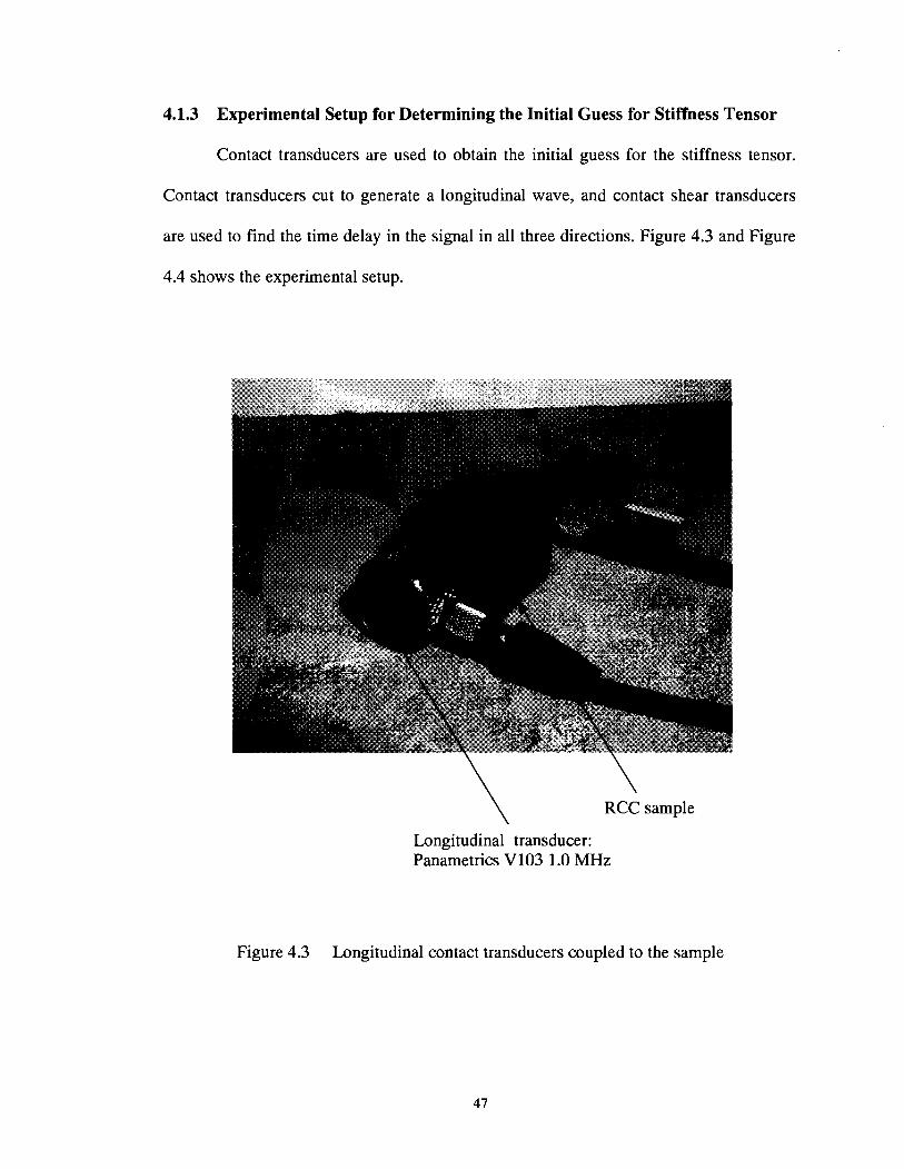
4.1.3 Experimental Setup for Determining the Initial Guess for Stiffness Tensor

Contact transducers are used to obtain the initial guess for the stiffness tensor.

Contact transducers cut to generate a longitudinal wave, and contact shear transducers

are used to find the time delay in the signal in all three directions. Figure 4.3 and Figure

4.4 shows the experimental setup.

\ RCC sample

Longitudinal transducer: Panametrics V103 1.0 MHz

Figure 4.3 Longitudinal contact transducers coupled to the sample

e-glass vinylester \ sample Shear transducer:

Panametrics V15 1.0 MHz

Figure 4.4 Shear contact transducers coupled to the sample

Proper coupling is applied between the transducer and the sample to ensure the

good transmission of ultrasonic waves. For longitudinal transducers UT-30 ultrasound

couplant (Sonotech Inc) is used as a couplant and petroleum jelly is used as couplant for

shear transducers. The transducers are firmly pressed on to the measuring faces of the

sample by hand while recording the signal using an oscilloscope. The same procedure is

repeated for all the 3 faces using both longitudinal and shear transducers.

4.1.4 Experimental Setup for Determining the Effects of Oxidation on

Attenuation

The same samples used to obtain velocity data and attenuation data at room

temperature are used to obtain oxidation data. The samples are placed in a tube furnace.

The furnace is a conventional tube type, 3-zone furnace (Lindberg Model 55346,

Watertown WI) that has three individual embedded alloy heating elements (type LGO),

located near the center. The furnace is capable of producing temperatures up to 1100°

C. The three heating elements surround a 40mm outer diameter (32mm inner diameter)

mullite tube (Anderman Ceramics, model EWF .610, London UK) that runs horizontally

through the furnace extending out to the right and left hand sides. Alumina fiber

insulation also surrounds the mullite tube through the furnace.

Mullite tube

/ ,Heating element

\ 'RCC sample Alumina insulation

urnace casing

Figure 4.5 Photograph of the furnace with cross sectional details

The mullite tube allows the entire apparatus, shown in Figure 4.5, to be sealed

from the outside of the furnace. This allows the RCC composite to be held in a

controlled atmosphere furnace. Without the tube extending out of the furnace, sealing

the RCC sample inside a high temperature atmosphere is difficult.

4.2 Experimental Preparations and Procedures

Sample preparations and the procedure for the experiment is particularly critical

for the RCC because of the sample layup. In the RCC orientation of the sample is

critical. Similar samples are used for the polymer matrix composites, however

preparation is somewhat less critical.

The original block of RCC obtained through Applied Thermal Sciences (Sanford,

ME) was 124 mm x 122 mm x 41 mm (E 5 x 5 x 1.5 inches). Specimenss were cut from

this original block for a number of experiments. The specimens used in these tests were

cut from larger sections using a tile saw (MK diamond products, model MK101,

Torrance, CA). The opposing sides of the test specimens are cut as close to parallel as

possible in order obtain accurate data. The thickness of each specimen was cut to 9mm.

The height and width of the samples were cut to 25mm and 24mm respectively. The

thickness dimension is critical for the attenuation measure because of the direct effect as

well as changes in measured attenuation due to non-parallel faces. Keeping the overall

dimensions of all RCC composite specimens similar simplifies the experiments and

calculations. Each sample is marked to identify the orientation with respect to the

original block.

All of the specimen dimensions are carefully measured, accurate to O.Olmm,

recorded and placed in a small, labeled plastic bag. The bags were labeled with the date

that the sample was tested. Each specimen was weighed, using a tabletop scale (Davis

Instruments, model SV-200 Baltimore MD) accurate to 0.01 g. Once these specimens

were cut, measured and recorded, they were ready to be tested. e-glass vinylester

samples are cut from 460 mm x 30mm x 25mm composite beams to the same

dimensions as of the RCC samples.

The experimental procedure consists of two separate parts. First, a procedure for

obtaining the data required for extracting the elastic modulus and attenuation of e-glass

vinylester and RCC at room temperature. A separate procedure is required to perform

the controlled oxidation of the RCC samples.

4.2.1 Elastic Modulus and Attenuation Determination

One of the methods for obtaining velocity data in an ultrasonic immersion

technique is to compare the signal through the sample with a signal through the medium

without a sample. Measurements are performed with 4 incident planes, azimuthal angles

being o', 45', 90°, 135' associated at a range of different incident angles. In each of the

incident planes, 25 measurements were carried out corresponding to 25 incident angles

(0' to 24'). At each incident angle, the relative time delay was measured from the

signals received. Only the highest amplitude mode was measured. All the

measurements are conducted in a water tank where the temperatures are monitored

continuously. A reference signal is also recorded at the same water temperature. The

reference signal is obtained by removing the sample and allowing the ultrasonic signal to

travel directly from the transmitter to the receiver. Each of the data set consisting of 100

signals is compared with the reference signal to obtain the velocity data. To obtain the

attenuation and damping property only one of the data set, the one with azimuthal angle

and incident angle at 0' to the material principal axis is considered. This signal is

compared with the reference signal to obtain the attenuation.

4.2.2 Determination of Effects of Oxidation on Attenuation

For the controlled oxidation studies the samples are placed in the furnace and

heated to 700' C in an inert environment. Compressed nitrogen is used here. The

samples are maintained at 700' C for 45 minutes in an oxidizing environment allowing it

to oxidize, for this the nitrogen is disconnected and compressed air is supplied through

the furnace. Then the samples are removed and weighed. The oxidized samples are

tested in an immersion process as explained in section 4.1.1 for obtaining the attenuation

data, ie, azimuthal angle oOand incident angle 0' (one data set).

4.2.3 Experimental Determination of the Initial Guess Used in Stiffness Matrix

Algorithm

The determination of initial guess for the nonlinear optimization algorithm used

for recovery of the stiffness matrix is explained in this section. A cube of dimension

0.026 x 0.091 x 0.021 m is cut from the same RCC sample used for the recovery of the

tensor. The setup shown in section 4.1.3 is used. The time delay for longitudinal and

shear (transverse) waves are determined using the setup. A coordinate system as

illustrated in section 3 is followed for obtaining the initial guess. Longitudinal waves

transmitted through thickness in 1, 2 and 3 directions yield El, E2 and E3 respectively.

This is explained in detail in section 3.3.2. Time delays are recorded in each of these 3

directions and the longitudinal wave speed is calculated as:

Thickness of sample in direction of measurement C , =

time delay

A similar method is followed with a shear wave transducer. The time delay

measured in different directions yield G23, G13 and G12 respectively. When the shear

transducer is placed in the 1 direction both G13 and G12 can be determined from the time

delay measured and the transducers aligned in the 2 direction recovers G23. This is

explained in detail in section 3.3.2. In this case, also, the shear wave speed is calculated

as:

Thickness of sample in direction of measurement c , = 4.2

time delay

For calculation purposes Poisson's ratios, v12, v13 and v2,is assumed to be 0.3

and the Maxwell-Betti reciprocal theorem is followed. This method is used to obtain the

initial guess for the RCC samples only, initial guess for e-glass vinylester is obtained

from a reference paper [Peterson, et al., 20021. The ultrasonic signals obtained using the

contact transducers are attenuated more in the case of e-glass vinylester making it

difficult to do analysis.

5 SIGNAL PROCESSING

In order to obtain engineering properties from ultrasonic testing, significant

signal processing is required. To obtain the time delay required for elastic modulus,

very high accuracy is required. The measurement of attenuation requires that the effects

of the instrumentation be removed from the measurement. Finally in order to obtain the

full compliance tensor from the multiple velocity measurements, a technique is required

to extract 21 constants from 100 equations. These techniques are described in the

following section.

5.1 Cross-correlation

To obtain accurate relative time delays cross-correlation is used [Peterson, 19971.

Cross-correlation algorithms are used to estimate the time delay difference (z) between

two signals. In this thesis an ultrasonic waveform transmitted through water (the

reference signal) is compared to a signal through the RCC sample. Cross correlation

techniques have broad applications in radar, digital communications and other areas in

science and engineering.

Assume two time domain signals to determine the time delay, x(n) and y(n) are

available that are sampled at discrete even time intervals n. The samples are evaluated

at discrete intervals and satisfy all discrete time sampling constraints. The cross

correlation between these two signals is defined by [Silvia, 19861

where z is time shift or time delay parameter and the subscript xy indicates the signals

used in the cross-correlation. The inner product of two vectors in a finite dimensional

domain is [Silvia, 19861

where 0 I n I N - 1 is the domain of interest.

Let y(n) = x(n -z) in equation 5.2. When z=0, signal x(n) and x(n - z) are

identical. The inner product (equation 5.2) is at a maximum. In general, the shift

parameter between two signals always occurs at the peak of cross correlation.

Compared to equation 5.2, the cross correlation (equation 5.1) is actually the inner

product of x(n) and y(n) , which is a function of shift parameter z. Therefore, the cross

correlation, like other inner products, measures the degree of similarity between two

signals. In general, the cross correlation function is neither symmetrical, nor unimodal

[Silvia, 19861. Examples of this in ultrasonics show methods to select peaks [Sun,

The cross correlation is used to measure the relative time delay to a reference

signal that results from the elastic wave propagation through a water path. An unknown

signal, which is from the wave that propagates through the sample, is compared to this

known signal. The relative time delay is determined by locating the time at which the

cross-correlation r,, is at a maximum. This is the point when the signals are most

similar. The average group velocity V of the ultrasonic waves propagating through the

sample can be estimated by [Hosten, 20011, as explained in section 3.3.1

VO

2 cos 8,

where Vo is the wave velocity in the water, zi is time delay, €Ii is the incident angle, d is

the thickness of the sample, and (xl, q) indicates the wave incident plane.

It is important to note that the use of the cross correlation results only in a

measure of the relative difference in the velocity. Therefore, the cross correlation can be

used to determine the difference in wave velocity between the reference sample and the

unknown sample. For the range of velocities considered, the only geometrical

dispersion that would only impact the measurement exists if large differences in the

phase velocities present between the unknown and the reference signal [Peterson, 19971.

As a result, unlike absolute measurements of velocity even in finite specimens, the effect

of dispersion can be assumed to be minimal.

5.2 Attenuation Measurement

It is necessary to use deconvolution to remove the effects of the measurement

system to allow determination of the attenuation of the ultrasonic wave propagating

through the sample. Consider the configuration shown in Figure 5.1 [Schmerr, 19981.

In order to separate the effect of the sample on the ultrasonic wave, it is necessary to

remove the response of the transducers and the rest of the measurement system from the

test.

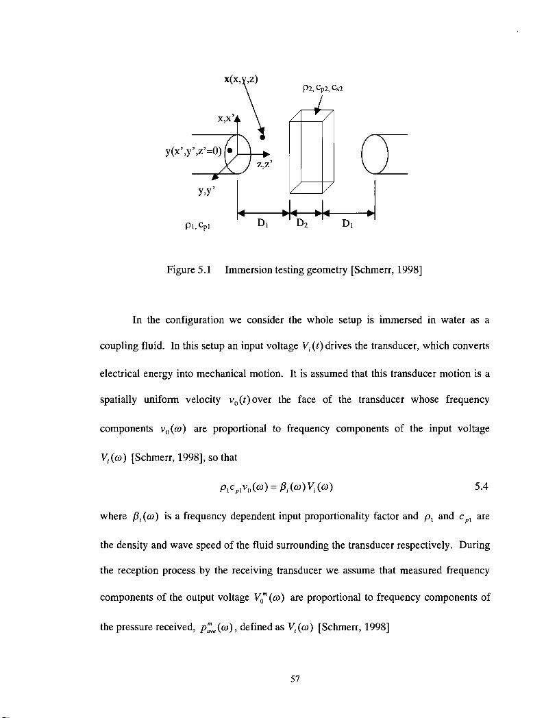
4 b PI, $1 D 1 D 1

Figure 5.1 Immersion testing geometry [Schmerr, 19981

In the configuration we consider the whole setup is immersed in water as a

coupling fluid. In this setup an input voltage V , (t) drives the transducer, which converts

electrical energy into mechanical motion. It is assumed that this transducer motion is a

spatially uniform velocity vo(t)over the face of the transducer whose frequency

components vo(w) are proportional to frequency components of the input voltage

V , ( a ) [Schmerr, 19981, so that

~lc,lvo ( 4 = Pi ( 4 V , ( a ) 5.4

where Pi(@) is a frequency dependent input proportionality factor and p, and c,, are

the density and wave speed of the fluid surrounding the transducer respectively. During

the reception process by the receiving transducer we assume that measured frequency

components of the output voltage V t ( o ) are proportional to frequency components of

the pressure received, p:, (a), defined as V , ( o ) [Schmerr, 19981

where p (Z,w) is the pressure on the transducer face and S is the surface area of the

transducer face. The above expression can also be written in terms of ideal received

pressure pave ( w ) as V , (a) [Schmerr, 19981

where ai and di are attenuation coefficients and corresponding path lengths followed

by waves in the ith medium while travelling from the transmitter to the receiver. This

decomposition is made so that pave(w) is separated from the attenuation terms. The

frequency components of the measured output voltage V , ( w ) can be written as Vi ( w )

[Schmerr, 19981

where pr ( w ) is a receiving proportionality factor. Combining equations 5.4 and 5.7 we

get V, (a) [Schmerr, 19981

where P(w) is single total efficiency factor

P ( a ) = Pi ( w ) P r ( w ) V , (a) 5.9

Using the general model, specific to the configuration in Figure 5.1 for measuring

material attenuation [Schmerr, 19981 for both front and back surface responses we have

~, l ' and v$are measured output voltages of the front surface and back surface

respectively. a, and a, are attenuation coefficients for the water and the solid.

p(o) is a receiving proportionality factor. The terms pLe and are spatially

averaged received pressure for the front-surface and back-surface, and vo is the

frequency response of the spatially uniform velocity over the face of the transducer. The

density and wave speed of the fluid surrounding the transducer are pl and Dl is the

distance between the transducer and sample, and D2 represents the thickness of the

sample [Schmerr, 19981. It is assumed that both front and back responses are measured

with the same transducer and at the same system settings, so that the efficiency factor is

the same in both cases. In principle we can obtain the attenuation of solid from Equation

5.10 by simply dividing the magnitudes of the back and front surface responses to obtain

[Schmerr, 19981

where

RgP, and TgZP denote the reflection coefficient from fluid to solid, the transmission

coefficient from fluid to solid, and the transmission coefficient from solid to fluid,

respectively. All of these three coefficients denote the transmitted longitudinal wave

due to an incident longitudinal wave. Dl is a diffraction correction term, and

kpl = w/cp l . An example of results of using such an approach for a block of aluminum

is shown in Figure 5.2, where over a frequency range of 6-10 MHz, the attenuation

variation can be fit to linear function as

Frequency (MHz)

Figure 5.2 Attenuation coefficient as measured for an aluminum block and the best fit

straight line for values in the bandwidth of the transducer (approximately 6-10 MHz)

[Schmerr, 19981

In this thesis equation 5.12 is used to calculate a, from the measured signals

B(w) and F(w) . Plotting of the attenuation function is not done in this thesis.

5.3 Constrained Optimization

The next key element to the processing of the data is the optimization used to

extract elastic constants from 100 experimental data sets. In general optimization arises

whenever there is an objective function that must be tuned for optimal performance.

Constrained optimization is the minimization of an objective function subject to

constraints on the possible values of the independent variable. Constraints can be either

equality constraints or inequality constraints. In this thesis, optimization is used to find

the compliance tensor from velocity data measured in composite materials. The elastic

constants are reconstructed from a large number of wave velocity data points, by

performing Newton-Raphson non-linear optimization. The equation for optimization is

IT, -g i jpv 1 = o 5.16

Three phase velocities corresponding to the three wave modes form the three solutions

of this non-linear cubic equation (equation 3.18). Every measured phase velocity, V, is

approximately the solution of equation 5.16.

f(v,,, C, )= lrij -sijpv21- o 5.17

where f K,, , Cij) is the left hand side of the equation 5.16 and Vex, (n) indicates the

phase velocities measured from the four incident planes as described in section 4.

Reconstruction of all 21 components of Cij can be performed by minimizing an objective

function F (C,) , which is the sum of squares of equation 5.16.

C, = min (F (c, ))

with

where n represents all data points collected from the four incident planes.

Equation 5.19 shows that the method minimizes the effect of random deviations

of experimental data on the results of reconstruction. The wave velocity measurements

are indeed embodied in each objective function to be minimized. There are more

experimental data points than the number of the independent elastic constants.

Therefore Equation 5.17 is constructed from an over-determined system of the functions

f (V,,,, Cij ) [Every and Saches, 19901. Contrary to another method that considers the

direct solutions of Christoffel's equation [Rokhlin and Wang, 19921, this minimization

problem requires no mode distinction [Aristegui and Baste, 19971. This is simply

because each of the modes generated is the solution of Christoffel's Equation and should

satisfy Equation 5.16. For the general case, the velocity data are collected from four

incident planes o', 45', 90' and 135' associated with various incident angles.

The minimization was performed by using a standard MATLAB optimization

function, which is based on the Newton-Raphson method described above. A successful

implementation of optimization requires reasonable estimates of the elastic constants as

initial values to feed into the algorithm. The determination of initial values was earlier

explained in section 4.2.1.3.

The following steps leads to the reconstruction of the elastic constants Cij using

the optimization technique:

A set of phase velocities Vex, (I), ... Vex, (n), which correspond to each of these wave

modes, is measured from four incident planes. Twenty-five different incident angles

are needed at each of the four incidental planes to make up a total of 100 data points.

Using a trial set of elastic constants cOij as an initial guess to construct a

f ' (Vex,, c,; ) , and an objective function F ' (C, j ) to be minimized through

Equation 5.17 and Equation 5.19.

At each step (kth) of the iteration, an error e, , which is defined as the difference

between the cijk and the desired Cij, will result. The closer the cijk are to the Cij, the

smaller, on the average, the error will be.

This procedure may be iterated until

ek - ek_, = c.!~) - 5 E 11 11

5.20

where E is a pre-assigned tolerance of a very small quantity. An example is shown in the

appendix.

6 RESULTS

This section provides summary results for the data obtained for the thesis and

additional data may be found in the appendix. The coordinate system defined in section

3.3.1 is used in the discussion.

6.1 Results for Recovered Elastic Stiffness Tensor and Principal Coordinate

System

6.1.1 Results for RCC

The initial guess used in the recovery of the elastic tensor from the ultrasonic

data is obtained experimentally as illustrated in section 4.2.2.3 and is used in the

recovery of the elastic stiffness tensor from the velocity data.

Initial guess, C =

An example of the stiffness tensor reconstructed from the above initial guess using the

velocity data is, stiffness tensor, C =

The eigenvalues of C is

The reconstructed stiffness tensor has off diagonal terms which are represented

as zeros but negative. These represent significantly small negative numbers in the

tensor. The numbers are so small that they are assumed to be zero. As introduced in

section 3.3.2, the principal coordinate system R' with respect to the observation

coordinate system R can be located by determining a set of Euler's angle unknowns

6=(a, p, y) with at least one of the unknown is zero [Auld, 1990; Aristegui and Baste,

19971. For the stiffness tensor above, the Euler angles were determined to be

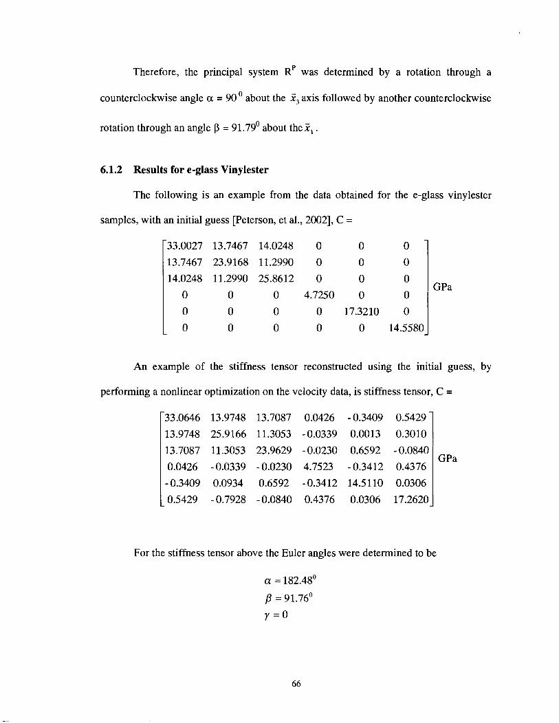
Therefore, the principal system R' was determined by a rotation through a

counterclockwise angle a = 90 O about the I, axis followed by another counterclockwise

rotation through an angle P = 91.79' about the?, .

6.1.2 Results for e-glass Vinylester

The following is an example from the data obtained for the e-glass vinylester

samples, with an initial guess [Peterson, et al., 20021, C =

- 33.0027 13.7467 14.0248 0 0 0

13.7467 23.9168 11.2990 0 0 0

14.0248 11.2990 25.8612 0 0 0

0 0 0 4.7250 0 0

0 0 0 0 17.3210 0

0 0 0 0 0 14.5580 -

GPa

An example of the stiffness tensor reconstructed using the initial guess, by

performing a nonlinear optimization on the velocity data, is stiffness tensor, C =

For the stiffness tensor above the Euler angles were determined to be

GPa

Data was collected form a sample, which was cut at an angle of 5 degrees from

the xz direction. This was done in order to check the optimization routine. The

reconstructed stiffness tensor, for this sample, C =

For the stiffness tensor above the Euler angles were determined to be

Additional results are included in the appendix

6.2 Results for Damping Characteristics

Following selection of the principal axes of the sample it is now possible to

measure damping using the one-dimensional theory presented in section 3. The

damping characteristics of various samples and the repeatability of the process are

considered. The following curves show the damping versus frequency characteristics

for samples of RCC and e-glass vinylester. Repeatability of the experimental process is

demonstrated in fig 6.2 and fig 6.4. Care was taken to make sure that the sample

positioning on the sample holder was identical for all samples. Even though there are

differences in the curves, all of them show the same trend. More data are plotted in the

appendix section. A smoothed curve is also shown in the appendix section, which gives

a better idea about the trend of these curves.

6.2.1 Results for RCC

* Sample B + Sample C

Figure 6.1 Damping characteristics of RCC, 2, direction for 3 specimens cut from the

same sample

0 Run I * Run 2 + Run 3

Run 4

Figure 6.2 Repeatability of damping characterization of RCC, using the same sample

in 4 different tests on different days under same conditions and same orientation

6.2.2 Results for e-glass Vinylester

Figure 6.3 Damping characteristics of e-glass vinylester, 2, direction70

* Run 2 Run 3

Figure 6.4 Repeatability of damping characterization process of e-glass vinylester,

over 3 different runs'on 3 different days under same conditions and same orientation

0.5

0.45

0.4

0.35

- 0.3 m + - -8 0.25 V

C m +

0.2

0.15

0.1

0.05

0

-

-

-

-

- El

- 0

# 0 * E l

- #

0 0

- 0 0 #

- Q4

-

I I I I I

0.3 0.4 0.5 0.6 0.7 0.8 Frequency ,MHz

6.3 Effect of Oxidation on Damping

To study the effects of oxidation on damping of RCC samples, the difference in

tan(6) of the same sample before and after oxidation is studied at various frequencies.

Five samples were considered with each oxidized to a different weight loss percentage.

Figure 6.3 shows the variation in damping characteristics for samples oxidized to

different levels.

2.21% 5.24% 6.85% 7.11% 21.13%

Weight Loss

Figure 6.5 Attenuation changes during oxidation

7 DISCUSSIONS, CONCLUSION AND FUTURE WORK

From the results shown is section 6 it is clear that the measurement technique

and the optimization routine used to recover the stiffness tensor from experimental data

is working as expected. The recovered stiffness tensor is almost identical to the initial

guess obtained using the contact method. This was expected since for both RCC and e-

glass vinylester the samples were cut from a large composite sample. It was also

demonstrated in the results that the composite samples are oriented with the principal

axis and variability within 5'. This means for design it can be assumed orthotropic and

simple measurements could be made with ultrasonic or other mechanical methods.

7.1 Stiffness Tensor recovered for RCC

For RCC the vector of eigenvalues is positive definite, which is a constraint on

the optimization. Closer analysis of the initial guess and the recovered tensor for RCC

in section 6.1.1 shows us that optimization routine found the minimum by flipping some

of the terms. This is reasonable since it was possible that, while cutting the sample from

the block for this particular experiment the orientations were switched with respect to

the orientations of the sample used to find the initial guesses. When the optimization

routine found the optimized value, it was in effect just changing the values in the 2, and

iZ direction. The optimization routine ended up turning the axes by approximately 90'

in the a and p directions, thereby orienting the samples in the same direction. For the

composite samples we consider the initial guess to be in the principal axis

7.2 Stiffness Tensor recovered for e-glass Vinylester

The e-glass vinylester sample used in data collection was mis-oriented by 1.5" in

the XI direction and 0.79" in the x2 direction (section 6.1.2). Figure 7.1 illustrates this.

Figure 7.1 Orientation of the e-glass vinylester sample with respect to principal axis

Stiffness tensor recovered from the e-glass vinylester sample cut at an angle of 5

degrees off from the x2 direction, was as expected. The Euler angle /? was calculated to

be 7.16"' This supports the optimization routine used to recover the stiffness tensor.

7.3 Damping Measurements and Oxidation Effects

The composite samples are oriented with the principal axis and varibility within

5". The damping measurements were estimated with this variability. This was done

because the variability is too small to cut the sample in the new orientation.

Repeatability of the damping measurements is also acceptable with less than 10%

variability. Improvements are needed to match design and evaluation state of matrix.

The attenuation changes during oxidation shown in Figure 6.5 shows similarity

in trend with the initial results discussed in section 1.1.1. The difference in tan 6

measurements for higher frequencies 0.75 MHz, 0.70 MHz and 0.63 MHz shows a

decrease as oxidation is increased (increase in weight loss %). The two lower

frequencies tend to have a wavy characteristic. This data is not suitable for designing

until the damping accuracy is good.

7.4 Future Work

More work has to be done in the future to improve the techniques explained and

developed in this thesis. The source of the variability in damping should be established.

It can be due to boundary conditions, sample size, or the electronics used. Even though

an efficient optimization routine is used, there are better techniques to tackle the

problem [Venkataraman, 20021. All these advanced optimization routines were not used

in this thesis since they are beyond the scope of this research. Use of a better

optimization package like TOMLAB' is also suggested.

REFERENCES

Achenbach, J. D. 1984. Wave Propagation in ElasticSolids. Amsterdam: Elsevier

Science Publishers B.V.

Anastasi, R.F., Friedman, A., Hinders, M., and Madaras, E. 1998. NDE of damage in

thick stitched composites using laser based ultrasound with optical fibers for

remote generation and detection. Material Evaluation, Vol. 56. No 12.

Aristegui, C. and Baste S. 1997. Optimal determination of the material symmetry axes

and associated elasticity tensor from ultrasonic velocity data. Journal of the

Acoustical Society ofAmerica. Vo1.102.

Aristegui C. and Baste, S. 2000. Determination of the elastic symmetry of a monolityic

ceramic using bulk acoustic waves. Journal of Nondestructive Evaluation. Vol.

19.

Auld, B. A. 1990. Acoustic Fields and Waves in Solids. Malabar: Krieger Publishing

Company.

Baudouin, S. and Hosten, B. 1997. Comparison between prediction and measurement of

viscoelastic moduli in composite materials versus temperature using ultrasonic

immersion technique with oil. Journal of the Acoustical Society of America, Vol.

102. No 6.

Bicerano, J. 1993. Prediction of Polymer Properties. New York: Marcel Dekker Inc.

Birman, V and Byrd, L. W. 2000. Review of Fracture and fatigue in ceramic matrix

composites, ASME Review papers in Applied Mechanics, Vol. 53. No 6.

Bunker, S.P. 2002. Evaluation of Dynamic properties of Carbon-carbon Composite at

Elevated Temperatures. Master's thesis, University of Maine.

Chimenti, D.E. 1997. Guided waves in plates and their use in materials characterization.

Applied Mechanics Reviews. Vol. 50. No 5.

Christensen, R. M. 1971. Theory of Viscoelasticity: An Introduction. New York:

Academic Press.

Chu, Y. C., Degtyar, A.H., and Rokhlin, S. I. 1994. A method for determination of

elastic constants of a unidirectional lamina from ultrasonic bulk velocity

measurements. Journal of theAcoustica1 Society of America. Vol. 96.

Cowin, S. C. and Mehrabadi, M. M. 1987. On the identification of material symmetry

for anisotropic elastic materials. Quarterly Journal of Mechanics and Applied

Mathematics. Vol. 40.

Cowin, S. C. 1989. Properties of the anisotropic elasticity tensor. Quarterly Journal of

Mechanics and Appied Mathematics. Vol. 42.

Every, A. G. and Saches, W. 1990. Determination of the elastic constants of anisotropic

solids from acoustic-wave group-velocity measurements. Physics Review. Vol.

B42.

Fedorov, F. I. 1986. Theory of Elastic Waves in Crystals. New York: Plenum Press.

Fraga, A. N., Alvarez V. A., and Vazquez, A. 2003. Relationship between dynamic

mechanical properties and water absorption of unsaturated polyester and vinyl

ester glass fiber composites. Journal of Composite Materials. Vol. 30. No 17.

Fung, Y. C. 2001. Classical and Computational Solid Mechanics. Singapore: World

Scientific.

Gauthier, M.M. 1995. Carbon-Carbon Composites, Engineering Materials, Handbook

Desk Edition, Materials Park: ASM International.

Gehman, Jr., H. W., Barry, J. L., and Deal, D.W. 2003. Columbia Accident Investigation

Board Report. NASA. Vol. 1.

Grigoriev, I. S. and Meilikhov, E. Z. 1997. Handbook of Physical Quantities. New York:

CRC Press.

Hearmon, R. F. S. 1961. An Introduction to Applied Anisotropic Elasticity. London:

Oxford University Press.

Hellier, C. J. 2001. Handbook of Nondestructive Evaluation. New York: McGraw-Hill.

Hellwege, K. H. 1979. Numerical Data and Functional Relationships in Science and

Technology Vol. 11. New York: Springer-Verlag.

Hosten, B. 1991. Reflection and transmission of acoustic plane waves on an immersed

orthotropic and viscoelastic solid layer. Journal of the Acoustical Society of

America. Vol. 89.

Hosten, B. 2001. Ultrasonic Through-Transmission Method for measuring the complex

stiffness moduli of composite materials. Handbook of Elastic Properties Solids,

Liquids, and Gases. New York: Academic Press.

Hosten, B., Hutchins, D. A., and Schindel, D. W. 1996. Measurement of Elastic

Constants in Composite Materials Using Air-Coupled Ultrasonic Bulk Waves,

Journal of the Acoustical Society of America. Vol. 99. No 4.

Jenkins, C. H. 1998. Manual on experimental methods of mechanical testing of

composites. Lilburn: The Fairmont Press, Inc.

Jones, R. M. 1975. Mechanics of composite materials. New York: Hemisphere

Publishing Corporation.

Kimura, S., Yasuda, E., and Tanabe, Y. 1982. Microstructure and Fracture Behavior of

Unidirectionally Reinforced Carbon FiberlCarbon Composites. Progress in

Science and Engineering of Composites International Conference.

Krautkramer, J. and Krautkramer, H. 1975. Ultrasonic testing of materials (Third,

revised edition). New York: Springer-Verlag.

Mase, G. E. 1970. Schaum's Outline of: Theory and Problems of Continuum Mechanics.

New York: McGraw-Hill Book Co.

Menard, K. P. 1999. Dynamic Mechanical Analysis: A Practical Introduction. Boca

Raton: CRC Press.

Migliori, A. and Sarrao, J. L. 1997. Resonant ultrasound spectroscopy. New York:

Wiley.

Musgrave, M. J. P. 1970. Crystal Acoustics. San Francisco: Holden-Day, Inc.

Newman, J. W., 1996. Shearography. Non destructive testing for aerospace composites.

Trends in NDE science & technology; Proceedings of the 1 4 ~ ~ World conference

on non destructive testing. New Delhi.

Norris, A. N. 1988. On the acoustic determination of the elastic moduli of anisotropic

solids and acoustic conditions for the existence of planes of symmetry. Quarterly

Journal of Mechanics and Applied Mathematics. Vol. 42.

Papadakis, E. P., Patton, T., Tsai, Y. M., Thompson, D. O., and Thompson, R. B. 1991.

The elastic moduli of a thick composite as measured by ultrasonic bulk wave

pulse velocity. The Journal of theAcoustica1 Society ofAmerica. Vol. 89.

Peterson, M. L. 1997. A Method for Increased Accuracy of the Measurement of Phase

Velocity. Ultrasonics. Vol. 35. No 1.

Peterson, M. L., Sun, M., Senan, A., Horton, K., Radford, D. W., and Thompson, L.,

2002. Dynamic Materials Characterization of Marine Composites. 17th

Technical Conference, American Society for Composites. Lafayette.

Rokhlin, S. I. and Wang, W. 1992. Double Through-Transmission Bulk Wave Method

for Ultrasonic Phase Velocity Measurement and Determination of Elastic

Constants of Composite Materials. Journal of the Acoustical Society of America.

Vol. 91. No 6.

Savage, G. 1993. Carbon-Carbon Composites. London: Chapman & Hall.

Schrnerr, Jr., L. W. 1998. Fundamental of Ultrasonic Nondestructive Evaluation; A

Modeling Approach. New York: Plenum Press.

Schreiber, E., Aderson, O., and Soga, N. 1973. Elastic Constants and Their

Measurements. New York: McGraw-Hill.

Shames, I. H. 1966. Engineering Mechanics Vol. II Dynamics. New Jersey: Prentice-

Hall, Inc.

Silvia, M. T. 1986. Handbook of Digital Signal Processing: Time Delay Estimation

Chapter 11. New York: Academic Press, Inc.

Strobl, G. 1996. The Physics of Polymers: Concepts for understanding their Structures

and Behavior. New York: Springer.

Summerscales, J. 1990. Non-destructive testing of fiber-reinforced plastic composites

Vol. 2. New York: Elsevier Science Publishing Co., Inc.

Sun, M. 2002. Optimal recovery of elastic properties for a general anisotropic material

through ultrasonic measurements. Master's thesis, University of Maine.

Venkataraman, P. 2002. Applied Optimization with MATLAB Programming. New York:

John Wiley & Sons.

Zweschper, T., Dillenz, A., Riegert, G., Scherling, D., and Busse, G. 2003. Ultrasound

excited thermography using frequency modulated elastic waves, Insight - Non-

Destructive Testing and Condition Monitoring, Vol. 45. No 3.

APPENDICES

Appendix A - MatLab Routines

Optimization Routine Used to Recover the Stiffness tensor

Following are the MATLAB routines and functions used to obtain the elastic

tensor from the velocity data.

clear; format('short'); %initial guess guess-ec=[121.3977 45.8033 50.1603 0 0 0;

45.8033 69.8789 34.7046 0 0 0; 50.1603 34.7046 105.0708 0 0 0; 0 0 0 27.6067 0 0; 0 0 0 0 16.5485 0; 0 0 0 0 0 26.5371]*10A9;

%Input Options %Tolerances and Iteration limits can be set using this %options=optimset('MaxFunEvals',18000,'MaxIter',1000,'MaxPCGIter', 1000,'LargeScale','on',TolX',le+7 ,TolCon',le+7); ............................... Optimization ................................. % (@Get-object-F-eg-b -- Our function which takes in an initial value for EC & % computes through and gives out the velocities obtained to give a better EC %guess-ec -- Initial value of EC %O -- Minimum value possible for any entry in the EC matrix %14*10A9 -- Maximum value possible for any entry in the EC matrix %options -- Sets the tolerences and maximum iteration values for optimization ................................................... ........................... %EC~arbiary=lsqnonlin(@Gettobject~F~eg~b,guess_ec,-O.O00Ol ,129* 10A9,0ptions);

[vec-A,D-A] =eig(A); [vec-B,D-B]=eig(B); for i=1:3

AdotB=dot(vec-A($), vec-B(:,i)); ampA=(sum((vec~A(:,1))."2))".5; ampB=(sum((vec~B(:,1))."2))".5; Agl(i)=acos((AdotB)/(ampA*ampB))* 180Ipi;

end

for i=1:3 alfa(i)=acos(a(l ,i)); if sin(alfa(i))==O

beta(i)=0.0001; else beta(i)=acos((-a(2,i))/sin(alfa(i))); check(i)=sin(alfa(i))* sin(beta(i)); alfa(i)=alfa(i)* l801pi; beta(i)=beta(i)* l801pi;

end end

%%%%%%%%%%%%%%%%%%%%%%%%%% .......................... %find EC in principal coordinate system Agl-x=Euler_beta*pi/180; Rota-X=[l 0 0;

0 cos(Ag1-x) sin(Ag1-x); 0 -sin(Agl-x) cos(Ag1-x)];

Rota-Z=[cos(Agl-z) sin(Ag1-z) 0; -sin(Agl-z) cos(Ag1-z) 0; 0 0 11; %rotate about the z anix with clockwise 30

a=Rota-Z; a_Sq=a."2;

Function Used in the Optimization Routine function F=Get-object-F-eg-b(guess-ec) %This is a function intents to generate an object function for determination the elastic constants. %F is based on the Christoffel's Equation

load d:\Usr\Anish\Research\Data\check\eglass\rnl\sampleb\egb~velocityXO.dat; load d:\Usr\Anish\Research\Data\check\eglass\rn1\sampleb\egb~velocityX45.dat; load d:\Usr\Anish\Research\Data\check\eglass\elocityX9O.dat; load d:\Usr\Anish\Research\Data\check\eglass\rnl\sampleb\egb~velocityXl35.dat;

m=length(egb-velocityXO); Agl= [O:m] '; Alfa=[Agl; Agl; Agl; Agl]*pi/l80; Density=2019.471308; %Kg/mA3

for i=1:4*m

index-Beta= l+floor((i-1)/25); n l(i)=sin(Alfa(i))*cos(Beta(index-Beta)); n2(i)=sin(Alfa(i))*sin(Beta(index-Beta)); n3(i)=cos(Alfa(i));

end

c=guess-ec; for i=1:100

T(l,l)=(nl(i)" 2*c(l,l)+n2(i)"2*~(6,6) +n3(i)"2*~(5,5)+2*n2(i)*n3(i)*c(5,6)+ 2*n3(i)*nl(i)* c(1,5)+2*nl(i)*n2(i)*c(l,6))-RL_V_Sqr(i);

T(l,2)=nl(i)"2*~(1,6)+n2(i)"2*~(2,6)+ n3(i)"2*~(4,5)+n2(i)*n3(i)*(c(4,6)+~(2,5))+ n3(i)*nl(i)* (~(1,4)+~(5,6))+nl(i)*n2(i)*(c(l,2)+~(6,6));

T(2,1)=T(1,2); T(1,3)=nl(i)"2*~(1,5)+n2(i)"2*~(4,6)+ n3(i)"2*~(3,5)+n2(i)*n3(i)*(c(4,5)+ c(3,6))+n3(i)*nl(i)*

(~(1,3)+~(5,5))+nl(i)*n2(i)*(c(1,4)+~(5,6)); T(3,l)=T(l,3); T(2,2)=nl(i)"2*~(6,6)+n2(i)"2*~(2,2)+ n3(i)"2*~(4,4)+2*n2(i)*n3(i)*c(2,4)+ 2*n3(i)*nl(i)*

c(4,6)+2*nl (i)*n2(i)*c(2,6)-RL-V-Sqr(i); T(2,3)=nl(i)"2*~(5,6)+n2(i)"2*~(2,4)+ n3(i)"2*~(3,4)+n2(i)*n3(i)*(c(4,4)+ c(2,3))+n3(i)*nl(i)*

(~(3,6)+~(4,5))+nl(i)*n2(i)*(c(2,5)+~(4,6)); T(3,2)=T(2,3); T(3,3)=nl(i)"2*~(5,5)+n2(i)"2*~(4,4)+ n3(i)"2*~(3,3)+2*n2(i)*n3(i)*c(3,4)+ 2*n3(i)*nl(i)*

~(3,5)+2*nl(i)*n2(i)*c(4,5)-RL_V_Sqr(i); F(i)=det(T);

end

Routine Used to Determine the Velocities from Experimental Data clear; %Reference signal load d:\USR\Anish\Research\Data\check\eglass\~n5~lO\xO\water~ref.out; ref=water_ref(:,2); n=length(ref); V-ref=1485.7; %pick up the lowest sound speed in water, unit:m/s Thickness=0.008788; %thickness of the sample, unit:m timearray=water-ref(:,l); interval=timearray(2)-timearray(1);

%Input first data file load d:\USR\Anish\Research\Data\check\eglass\~n51O\xO\A100.out; input(:, 1)=A100(:,2);

%Input rest of the data files fileNumber=24; for i=l :fileNumber

fileName=sprintf('%s%02d.out','d:\USR\Anish\Research\Data\check\eglass\~n5lO\xOl',i); fileContent=load(fileName); input(:,i+l)=fileContent(:,2);

end

%Cross-correlation for p=1:25

for m=2:n shifty l=[input((m:n),p);zeros(m-l,l)];

crol(p,m)=dot(ref,shiftyl); shift-y2=[ref(m:n);zeros(m-l,l)]; cro2(p,m)=dot(input(:,p),shifty2); end crol(p,l)=dot(ref, input(:,p)); cro2(p,l)=dot(input(:,p), ref);

if y b y 2 y(p)=yl; index y(p)=-il; cro(p,:)=crol(p,:);

else Y(P)=Y~; index y(p)=i2; cro(p,:)=cro2(p,:);

end

%%%Calculate velocities velocity(p)=V~ref/(1+V~ref*delay(p)~ickness*(V~ref*delay(p)~ichess-2*cos(Agl(p))))A.5; velocityl(p)=[(delay(p)~hickness)A2-2*delay(p)*cos(~l~))/(V~ref*~ichess)+(l~~ref)A2]A(-.5);

end velocity; %index y fid=fopen('d:\USR\~nish\Research\Data\check\eglass\~n5lO\ega~velocityXO.dat',~'); fprintf(fid,'%16.12f\n',velocity); fclose(fid);

Sample Data File

I Time (s) I Voltage I

Table A.l Sample data file recorded using the oscilloscope

Appendix B - More Results and Smoothened Damping Curves

This section gives an account of various results obtained throughout the research

period for stiffness tensor

Experiment date: 25/06/03

Sample: RCC 1A

Euler angles, /3 = 89.36'

y = O


Sample: RCC 2B

Euler angles, /3 = 89.75'

y = o

GPa

GPa


Sample: RCC 3B

a = 88.62'

Euler angles, P = 89.75'

y = o


Sample: e-glass vinylester 1A


y = o

GPa

GPa


Sample: e-glass vinylester 2B

GPa

a = 182.68'


y = o

This section shows the smoothened curves of damping accuracy and damping

repeatability using a second-degree polynomial curve fit.

- Sample A - - Sample B - - - - - Samale C

Figure B.l Damping characteristics of RCC, x, direction, smoothened curve

Figure B.2 Smoothened curve showing repeatability of damping characterization

process, over 4 different runs on 4 different days under same conditions and same

orientation for RCC

Sample A Sample B

0 ' I I I I I I I I I

0.3 0.35 0.4 0.45 0.5 0.55 0.6 0.65 0.7 0.75 Frequency ,MHz

Figure B.3 Smoothened curve of damping characteristics of e-glass vinylester in x,

direction

Figure B.4 Smoothened curve showing repeatability of damping characterization

process, over 3 different runs on 3 different days under same conditions and same

orientation for e-glass vinylester

Thickness Oxidation Weight after Percentage after time (min) oxidation (g) Weight Loss Loss in weight oxidation

0 5.89 0.0 0.00% 0.00937

Sample No: 1 2 3 4

Table B.l Raw data for Figure 6.5, attenuation changes during oxidation

5 7.59 0.02057 0.02029 0.00978 6 7.62 0.02032 0.02007 ~ - 0.00996

Weight before oxidation (g)

5.89 5.89 5.73 5.55

Dimensions before oxidation (m)

Length 0.01 882 0.01 882 0.01 905 0.01 867

Breadth 0.01 781 0.01 781 0.01 854 0.01 854

Thickness 0.00937 0.00937 0.00841 0.00851

BIOGRAPHY OF THE AUTHOR

Anish Sen Senan was born in Trivandrum, Kerala, India on November 1, 1976.

He was raised in Trivandrum and graduated from Kendriya Vidyalaya High School in

1992. He attended the College of Engineering, Trivandrum (University of Kerala) for

his Bachelor's degree in Mechanical Engineering. He earned his Bachelor's in

Technology (B.Tech) degree in 1998. After graduation he worked as Materials-

Engineer, at Wipro Computers Ltd, India for 2 years. Later in 2000 he joined Acclaim

Systems, Inc as Business Development Manager. He came to the United States of

America in 2001 and started his graduate program in December 2001.

Anish is a candidate for the Master of Science degree in Mechanical Engineering

from The University of Maine in December, 2003.

Documents

Determination of the Viscoelastic Properties of General