Meccanica (2007) 42:293–306DOI 10.1007/s11012-006-9041-7

Identification of viscoelastic properties by meansof nanoindentation taking the real tip geometry into account

Andreas Jäger · Roman Lackner ·Josef Eberhardsteiner

Received: 24 July 2006 / Accepted: 13 November 2006 / Published online: 2 May 2007© Springer Science+Business Media B.V. 2007

Abstract Motivated by recent progress in visco-elastic indentation analysis, the identification ofviscoelastic properties from nanoindentation testdata taking the real tip geometry into account ispresented in this paper. Based on the elastic solu-tion of the indentation problem, the correspondingviscoelastic solution is obtained by the applica-tion of the method of functional equations. Thisgeneral solution, which accounts for the real geo-metric properties of the indenter tip, is specializedfor the case of a trapezoidal load history, com-monly employed in nanoindentation testing. Threedeviatoric creep models, the single dash-pot, theMaxwell, and the three-parameter model are con-sidered. The so-obtained expressions allow us todetermine viscoelastic model parameters via backcalculation from the measured load–penetrationhistory. The presented approach is illustrated bythe identification of short-term viscoelastic prop-erties of bitumen. Hereby, the influence of load-

A. Jäger (B) · J. EberhardsteinerInstitute for Mechanics of Materials and Structures,Vienna University of Technology, Karlsplatz 13/202,1040 Vienna, Austriae-mail: Andreas.Jaeger@tuwien.ac.at

R. LacknerComputational Mechanics, Technical University ofMunich, Arcisstrasse 21, 80333 Munich, Germanye-mail: Lackner@bv.tum.de

J. Eberhardsteinere-mail: Josef.Eberhardsteiner@tuwien.ac.at

ing rate, maximum load, and temperature on themodel parameters is investigated.

Keywords Nanoindentation · Creep · Bitumen ·Viscoelasticity · Mechanics of materials

1 Introduction

The main goal of nanoindentation (NI) is the iden-tification of mechanical properties of the indentedmaterial. During NI measurements, a tip withdefined shape penetrates the specimen surfacewith the indentation load P [N] and the penetra-tion h [m] recorded as a function of time. Com-monly, each indent consists of a loading, holding,and unloading phase (see Fig. 1). The hardnessof the material, defined as H = Pmax/Ac [Pa], isobtained from the loading phase of the NI test.Hereby, Ac [m2] is the horizontal projection ofthe contact area and Pmax [N] denotes the appliedmaximum load. According to [1,2], Young’s mod-ulus E of materials exhibiting elastic or elastoplas-tic behavior is obtained from the relation betweenthe measured initial slope of the unloading curveS = dP/dh|h=hmax and the indentation modulusM = E/(1 − ν2), reading

S = 2√π

M√

Ac, (1)

where ν is the Poisson’s ratio.

294 Meccanica (2007) 42:293–306

(a) (b)

Fig. 1 Illustration of (a) load history and (b) load–penetration curve of NI tests

Parameter identification of materials exhibiting,in addition to elastic and plastic material response,time-dependent behavior (e.g., polymers, bitumen,etc.) requires back calculation of the parametersfrom the holding phase of the measured pene-tration history h(t). Recently, analytical solutionsfor the indentation of axisymmetric, rigid tips intoa viscoelastic halfspace were reported in [3] forspherical tips and in [4] for perfect conical tips.

Whereas both [3,4] considered indenter tipscharacterized by exact geometric properties, theshape of real indenter tips varies in consequence ofthe production process and in the course of testingdue to attrition. By means of calibration, NI-testingequipment give access to the real tip geometry [2].In order to consider the so-obtained geometricalproperties of the tip for back-calculation of mate-rial parameters, analytical solutions for the inden-tation of a tip into a viscoelastic material, takingthe real tip geometry into account, are presented inthis paper. For this purpose, the geometrical repre-sentation of the indenter tip (with Atip = C0f (ρ)2

for perfect conical tips) is extended to

Atip(ρ) = ρ2π = C0f (ρ)2 + C1f (ρ), (2)

where Atip [m2] is the area of the cross section andρ [m] and f (ρ) [m] are the corresponding radiusand distance from the apex of the axisymmetrictip, respectively (see Fig. 2). C0 [–] and C1 [m] areconstants describing the tip shape, which are gen-erally provided during calibration of the NI-testingequipment. In a first step, we will solve the elasticindentation problem for the indenter shape givenin Eq. 2. According to [5], the viscoelastic solutionis obtained by replacing the operators of the elasticsolution by the Laplace transforms of the associ-ated viscoelastic operators. Back transformationgives access to the solution for viscoelastic inden-

Fig. 2 Contact between a rigid axisymmetric tip of shapef (ρ) and an infinite halfspace (P is the applied load, h is thepenetration, a is the contact radius, and Ac is the projectedarea of contact)

tation in the time domain. Finally, the viscoelasticsolutions are employed for the identification of vis-coelastic properties of bitumen from NI-test data.

2 Elastic indentation problem

For the solution of the elastic indentation prob-lem, i.e., a rigid indenter penetrating the elastichalfspace, the so-called Sneddon solution [1] is em-ployed. According to [1], the relation between thepenetration h [m] and the corresponding load P[N] is given for an axisymmetric indenter tip ofshape f (ρ) (see Fig. 2) by

h = a∫ a

ρ=0

f ′(ρ)dρ√

a2 − ρ2

P = 2E

1 − ν2

∫ a

ρ=0

ρ2f ′(ρ)dρ√

a2 − ρ2. (3)

Hereby, a [m] is the radius of the projected contactarea Ac, ρ [m] is the radius of the axisymmetrictip, f (ρ) [m] is a smooth function describing the tipshape, and f ′ = df/dρ.

Meccanica (2007) 42:293–306 295

For the case of conical indenters, f (ρ) = ρ/ tan α,where α is the semi-apex angle. Accordingly, forthe commonly used Berkovich indenter, whichmay be represented by a cone of α = 70.32◦, f (ρ)

becomes linear in ρ. In general, however, becauseof inaccuracies during the tip-production processand attrition, the aforementioned linear relationis nonlinear. During calibration of the NI-testingequipment, this nonlinearity is specified, followingthe procedure outlined in [2]:

1. Perform indents in a material with given elas-tic properties (e.g., fused quartz) in the depthrange of the indentation experiments;

2. Compute the projected contact areaAc = π/4(S/M)2, where S [N/m] is theinitial unloading slope of the load–penetra-tion curve and M is the indentation modulus,with M = E/(1 − ν2), where E = 72 GPa andν = 0.17 for fused quartz;

3. Plot Ac as a function of the contact depth hc,with hc = h − 0.75P/S, and approximate theso-obtained function by

Ac = C0h2c + C1hc, (4)

where C0 [–] and C1 [m] are constants describ-ing the tip shape.

Replacing Ac and hc in Eq. 4 by ρ2π and f (ρ),respectively, f (ρ) is obtained as

f (ρ) = 12C0

(√C2

1 + 4C0ρ2π − C1

). (5)

For the case of a conical indenter with a semi-apexangle α, where C0 = π tan2 α and C1 = 0, Eq. 5gives f (ρ) = ρ/ tan α. Figure 3 shows the tip-shapefunction f (ρ) and the area function Ac(hc) for aperfect Berkovich tip (C0 = 24.5 and C1 = 0) anda real Berkovich tip with a value of C1 deviatingfrom zero.

Inserting Eq. 5 into Eq. 3 gives the penetrationand the applied load as a function of the contactradius a,

h = a√

π

C0arctan

2a√

C0π

C1, (6)

P = 4πE

1 − ν2

2a3

3C12F1

(

1/2; 2; 5/2; −4a2C0π

C21

)

,

(7)

where 2F1(a; b; c; z) denotes a hypergeometricfunction, defined by (see, e.g., [6])

2F1(a; b; c; z) = �(c)�(b)�(c − b)

×∫ 1

0

tb−1(1 − t)c−b−1

(1 − tz)a dt, (8)

which is only valid for Re(c) > Re(b) > 0.

3 Viscoelastic indentation problem—applicationto trapezoidal load history

In the following, the elastic indentation problemoutlined in the previous section is extended to lin-ear viscoelasticity. For this purpose, the followingtwo methods may be employed:

1. Laplace transform method: The Laplacetransform method consists in removing thetime variable in the viscoelastic problem byemploying the Laplace transformation to thetime-dependent equations [7]. From the solu-tion of the so-obtained associated elastic prob-lem, the time-dependent solution is obtainedby application of the inverse Laplace transfor-mation. However, this method is restricted toproblems, where the interface between defor-mation and stress boundaries does not changewith time, which is not the case for indentationproblems.

2. Method of functional equations: In the caseof the considered indentation problems, themethod of functional equations, developed by[5], consists in replacing the elastic constantsin the solution of the equivalent elastic bound-ary value problem by the Laplace transformsof the associated viscoelastic operators. Thismethod is not restricted to fixed boundary con-ditions and remains valid as long as the contactarea increases monotonically with time [5].

Due to the restrictions of the Laplace transformmethod, the method of functional equations (seealso [3,4]) is employed to determine the visco-elastic solution for tip shapes described by Eq. 2.Hereby, the result for the solution of the indenta-tion in an elastic halfspace (Eq. 7) is rewritten inthe form

P = MF(a). (9)

296 Meccanica (2007) 42:293–306

(a) (b)

Fig. 3 (a) Tip-shape function f (ρ) and (b) area function Ac(hc) of a perfect Berkovich tip (C0 = 24.5 and C1 = 0), and a realBerkovich tip with C0 = 24.5 and C1 = 2314 nm

Thus, the solution is split into the material depen-dent indentation modulus M, with M = E/(1−ν2),and the function F(a) depending only on geomet-ric properties, such as the tip shape (representedby the constant parameters C0 and C1) and theunknown contact radius a, reading

F(a) = 4π2a3

3C12F1

(

1/2; 2; 5/2; −4a2C0π

C21

)

. (10)

Following the method of functional equations, theviscoelastic solution for the indentation problemis obtained by replacing the elastic operators P,M, and F(a) in Eq. 10 by their Laplace transformsP(s), M(s), and F(a(s)), giving

P(s) = M(s) F(a(s)). (11)

Re-arrangement yields an expression for theLaplace transform of the function F(a(s)) as

F(a(s)) = P(s)M(s)

= 1

sM(s)sP(s) = Y(s)sP(s) , (12)

where 1/(sM(s)) was replaced by the Laplacetransform of Y(t), in the following referred to asindentation compliance function. Considering that(i) a multiplication by s in the Laplace domain isequivalent to a derivation in the time domain and(ii) a multiplication of two Laplace-transformedfunctions is equivalent to the convolution productof the two functions in the time domain, F(a(t)) isobtained from Eq. 12 as

F(a(t)) =∫ t

0Y(t − τ)

ddτ

P(τ )dτ . (13)

Finally, combining Eqs. 10 and 13 allows determi-nation of the unknown contact radius a(t). Witha(t) at hand, Eq. 6 provides access to the history ofthe penetration, h(t).

The method of functional equations is restrictedto increasing contact areas, and may be appliedonly to monotonically increasing and constant loadhistories [5]. Since indentation tests are commonlyconducted under load control, Eq. 13 is specified tothe trapezoidal load history depicted in Fig. 1(a),reading

P(t) =

⎧⎪⎪⎪⎪⎪⎪⎨

⎪⎪⎪⎪⎪⎪⎩

PL(t) = t/τLPmax for 0 ≤ t ≤ τL,PH(t) = Pmax for τL ≤ t ≤ τL + τH

PU(t) = τL + τH + τU − tτU

Pmax

for τL + τH ≤ t≤ τL + τH + τU ,

(14)

where τL, τH , and τU are the loading, holding, andunloading durations, respectively. Considering theload history P(t) given in Eq. 14 in Eq. 13, the func-tion F(a(t)) becomes for the loading and holdingregime

FL(a(t)) =∫ t

0Y(t − τ)

ddτ

PL(τ )dτ

= Pmax

τL

∫ t

0Y(t − τ)dτ , (15)

Meccanica (2007) 42:293–306 297

(c)(b)(a)

Fig. 4 Viscoelastic deviatoric creep models considered inthis study: (a) the single dash-pot (DP), (b) the Maxwell(MX) model, and (c) the three-parameter (3P) model

FH(a(t)) =∫ τL

0Y(t − τ)

ddτ

PL(τ )dτ

+∫ t

τL

Y(t − τ)d

dτPH(τ )dτ

= Pmax

τL

∫ τL

0Y(t − τ)dτ . (16)

Based on FL and FH in Eqs. 15 and 16, the historyof the penetration, h(t), for the loading and holdingtime is determined in three steps:

1. The indentation compliance function Y(t)appearing in Eqs. 15 and 16 is determined forthe considered viscoelastic model;

2. FL(a(t)) and FH(a(t)) are computed using Eqs.15 and 16; and

3. The contact radius a(t) and, hence, viaEq. 6, the penetration h(t) are determinedby combining the expressions for FL(a(t)) andFH(a(t)) with Eq. 10.

In the following subsections, these three steps aredescribed in more detail.

3.1 Determination of the indentation compliancefunction Y(t)

The indentation compliance function Y(t) is deter-mined for three deviatoric creep models, i.e., (i)the single dash-pot (DP), (ii) the Maxwell (MX)model, and (iii) the three-parameter (3P) model(see Fig. 4). In the case of elastic material response,the indentation modulus M can be expressed by thebulk modulus k and the shear modulus µ0, reading

M = E1 − ν2 = 9kµ0/(3k + µ0)

1 − ((3k − 2µ0)/(6k + 2µ0))2

= 4µ03k + µ0

3k + 4µ0. (17)

By the way of application of the method of func-tional equations, the elastic constants k and µ0in Eq. 17 are replaced by the associated Laplace-transformed operators k(s) and µ(s), reading

M(s) = 4µ(s)3k(s) + µ(s)

3k(s) + 4µ(s), (18)

where k(s) = k for the case of deviatoric creeponly. The shear relaxation modulus, on the otherhand, is time dependent, and is given by (see, e.g.,[8]):

µDP(s) = (sL{JDP})−1 =(sL{t/η})−1 =sη, (19)

µMX(s) = (sL{JMX})−1 =(sL{1/µ0 +t/η})−1

=(

1µ0

+ 1sη

)−1

, (20)

µ3P(s) = (sL{J3P})−1

=(

sL{

1µ0

+ 1µv

[1−exp

(−µv

ηt)]})−1

=(

1µ0

+ 1µv +sη

)−1

, (21)

where L{•(t)} denotes the Laplace transforma-tion of •(t). Considering µ(s) of the different vis-coelastic models given in Eqs. 19–21 in Eq. 18andapplying the inverse Laplace transformation toY(s) = 1/(sM(s)), Y(t) is obtained as

YDP(t) = 14

{tη

+ 1k

[1 − exp

(−3k

ηt)]}

, (22)

YMX(t) = 14

{1µ0

+ tη

+ 1k

[1 − µ0

µ0 + 3k

exp

(− 3kµ0

η(µ0 + 3k)t)]}

, (23)

Y3P(t) = 14

{1µ0

+ 1µv

[1 − exp

(−µv

ηt)]

+ 3(µ0 + µv)

µ0µv + 3k(µ0 + µv)

×[

1 − µ20

(µ0 + 3k)(µ0 + µv)

exp

(−µ0µv + 3k(µ0 + µv)

η(µ0 + 3k)t)]}

. (24)

298 Meccanica (2007) 42:293–306

In the case of incompressible materials, where k =∞, Eqs. 22–24 simplify to

YDP(t) = 14

tη

, (25)

YMX(t) = 14

(1µ0

+ tη

), (26)

Y3P(t) = 14

{1µ0

+ 1µv

[1 − exp

(−µv

ηt)]}

. (27)

3.2 Determination of F(a(t))

Considering the indentation compliance functionsY(t) for the three viscoelastic models given inEqs. 22–24 in Eqs. 15 and 16, the function F(a(t))is obtained for the loading and holding regime,FL(a(t)) and FH(a(t)), for the three consideredviscoelastic models as

FL−DP(a(t)) = Pmax

τL

∫ t

0Y(t − τ)dτ

= Pmax

4τL

{1k

t + 12η

t2 − η

3k2

(1 − exp

(−3k

ηt))}

, (28)

FH−DP(a(t)) = Pmax

τL

∫ τL

0Y(t − τ)dτ

= Pmax

4τL

{τL

k+ 1

2η(2t − τL)τL + η

3k2

(exp

(−3k

ηt) [

1 − exp

(3kη

τL

)])}, (29)

FL−MX(a(t)) = Pmax

4τL

{µ0 + kµ0k

t + 12η

t2 − η

3k2

(1− exp

(− 3µ0k

η(µ0 + 3k)t))}

, (30)

FH−MX(a(t)) = Pmax

4τL

{µ0 + kµ0k

τL + 12η

(2t − τL)τL + η

3k2

(exp

(− 3µ0k

η(µ0 + 3k)t)

×[

1 − exp

(3µ0k

η(µ0 + 3k)τL

)])}, (31)

FL−3P(a(t)) = Pmax

4τL

{3µ2

0η

(µ0µv + 3k(µ0 + µv))2

(−1 + exp

(−µ0µv + 3k(µ0 + µv)

η(µ0 + 3k)t))

+ (µ0 + µv)(4µ0µv + 3k(µ0 + µv))

µ0µv(µ0µv + 3k(µ0 + µv))t + η

µ2v

(−1 + exp

(−µv

ηt))}

, (32)

FH−3P(a(t)) = Pmax

4τL

{(1µ0

+ 1µv

+ 3(µ0 + µv)

µ0µv + 3k(µ0 + µv)

)τL − η

µ2v

(exp

(−µv

ηt)[

−1 + exp

(µv

ητL

)])

− 3ηµ20

(µ0µv + 3k(µ0 + µv))2

(exp

(−µ0µv + 3k(µ0 + µv)

η(µ0 + 3k)t)

×[−1 + exp

(µ0µv + 3k(µ0 + µv)

η(µ0 + 3k)τL

)])}. (33)

3.3 Determination of a(t) and h(t)

The history of the contact radius, a(t), is ob-tained from combining the expressions for FL(a(t))and FH(a(t)) given in Eqs. 28–33 with Eq. 10.The so-obtained (nonlinear) expression for a(t) issolved numerically, employing a Newton-iterationscheme. With a(t) at hand, the history of the pen-etration, h(t), is given by Eq. 6 for a given loadhistory P(t) and the material model describing thebehavior of the viscoelastic half space.

3.4 Illustrative example

The developed mode of determination of thepenetration history h(t) provides insight into theinfluence of the tip shape on NI results, as illus-trated for a DP-type material in Fig. 5. According

Meccanica (2007) 42:293–306 299

to Fig. 5(a), the largest penetration is obtained forthe perfect Berkovich. Any variation of the inden-ter tip from the perfect Berkovich tip results ina reduction of the penetration. Figure 5(b) showsthe deviation of the penetration depth from theBerkovich response, giving deviations found in thetens of percent.

4 Application—identification of viscoelasticproperties of bitumen

4.1 Introductionary remarks

Bitumen is the binder material of asphalt anddetermines its complex thermo-rheological behav-ior which, at high temperatures (T > 135◦C), pro-vides the low viscosity of asphalt required for theconstruction and compaction process of high-qual-ity asphalt layers. During hot summer periods, thisviscosity should be significantly higher in order toavoid the development of permanent deformationsin asphalt pavements (rutting), requiring costlyrepair work and reducing the traffic safety. Thedesirable increase of viscosity from hot to mediumtemperatures (0 < T < 70◦C) is, on the otherhand, disadvantageous at low-temperatures(T < 0◦C), causing low-temperature cracking inasphalt pavements in consequence of thermal-shrinkage strains associated with cooling duringchanging weather conditions.

In general, the viscosity of bitumen is found todecrease linearly with increasing temperature inthe log(viscosity)–temperature diagram (see Fig. 6[9]). The viscosity and its change with increasingtemperature is influenced by several factors:

1. The chemical composition and the molecularweight distribution of the crude oil;

2. The so-called cut point, i.e., the temperatureduring the distillation process (the higher thecut point, the higher the viscosity), and airblowing after the distillation process (increaseof viscosity due to bitumen oxidation); and

3. The allowance of additives (commonly poly-mers).

In order to gain insight in the origin of the bitumenviscosity, the viscous properties of one chosen typeof bitumen (B50/70, see Table 1) are determined,

Table 1 Properties of considered type of bitumen (B50/70)

Penetration depth [1/10 mm] [10] 49Breaking point by Fraß [◦C] [11] −13Softening point [◦C] [12] 50.5

Elemental analysis [mass-%]Carbon 83.04Hydrogen 10.38Nitrogen 1.11Sulfur 5.05� 99.58

employing the parameter-identification procedureoutlined in the previous section.

4.2 Specimen preparation and test protocol

In addition to the identification of model parame-ters, the application of the so-called grid indenta-tion technique [13] gives access to the morphologyof bitumen in the µm range and allows applica-tion of statistical techniques for the interpretationof NI-test results. Hereby, several indents are per-formed on a specified grid (e.g., 10 × 10 indents).The distance between two adjacent grid pointsis adjusted to the characteristic dimension of thebitumen microstructure and the maximum pene-tration.

The bitumen samples were prepared by heatingand pouring into a sample holder. The bitumensurface obtained from pouring (as opposed tolow-temperature fracture) exhibits the appropri-ate smoothness for NI testing. Two studies wereperformed, focusing on

– The influence of the loading rate and the maxi-mum load on the determined model parametersand

– The temperature dependence of the modelparameters.

4.3 Presentation of results and discussion

In order to determine model parameters for bitu-men from NI data, the analytical solutions forFL(a(t)) and FH(a(t)) (see Eqs. 28–33) are special-ized for incompressible materials, i.e., for k = ∞,giving

FL−DP(a(t)) = Pmax

8τLηt2, (34)

300 Meccanica (2007) 42:293–306

(a) (b)

Fig. 5 Indentation of viscoelastic halfspace (DP-model with η=100 MPa s) for different tip shapes: (a) Penetration history ofthe holding period; (b) deviation of penetration depth from response obtained from perfect Berkovich indenter (C0 = 24.5;load history: Pmax = 10µN, τL = 0.5 s, τH = 10 s)

Fig. 6 Temperature dependence of the zero-shear-rate limiting viscosity for different types of bitumen [9]

FH−DP(a(t)) = Pmax

8η(2t − τL), (35)

FL−MX(a(t)) = Pmax

4τL

{1µ0

t + 12η

t2}

, (36)

FH−MX(a(t)) = Pmax

4

{1µ0

+ 12η

(2t − τL)

}, (37)

FL−3P(a(t)) = Pmax

4τL

{(1µ0

+ 1µv

)t

+ η

µ2v

[−1 + exp

(−µv

ηt)]}

, (38)

FH−3P(a(t)) = Pmax

4τL

{(1µ0

+ 1µv

)τL − η

µ2v

exp

(−µv

ηt)[

−1+ exp

(µv

ητL

)]}.

(39)

Taking into account that the MX and the DP modelare special cases of the more general 3P model, giv-ing the MX model for µv = 0 and the DP model forµv = 0, µ0 = ∞, the 3P model is employed in thefollowing for the identification of model parame-ters. Hereby, the error between the experimentally

Meccanica (2007) 42:293–306 301

(a) (b)

Fig. 7 Illustration of error between model response and NI-test data (holding period): (a) penetration history h(t) and(b) function FH

obtained function Fexp(a(t))1 for the holding periodand the analytical result given in Eq. (39) is min-imized by adapting the unknown shear moduli µ0and µv, and the viscosity η (see Fig. 7). The men-tioned error is defined by

R3P(µ0, µv, η) = e(µ0, µv, η)

u(40)

with

e2(µ0, µv, η) =n∑

i=1

[Fexp(ti) − FH−3P(µ0, µv, η, ti)]2

and u2 =n∑

i=1

F2exp(ti) , (41)

where n was set equal to 10. The error given in Eq.40 was minimized by adapting µ0, µv, and η, usinga simplex iteration [14]. With the model param-eters at hand, the history of the contact radius,a3P(ti), is determined from Eq. 10 using a New-ton-iteration scheme. Subsequently, h3P(ti) is com-puted from Eq. 6 (see, e.g, Fig. 7(a)). The procedureemployed for parameter identification is summa-rized in Fig. 8.

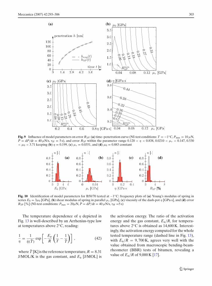
In order to check the existence of a global min-imum of the error R3P, the influence of the modelparameters on the error R3P is studied. Figure 9shows contour-plots of the error as a function of

1 Fexp(a(t)) is determined from the penetration history us-ing Eqs. 6 and 10 and C0 = 24.5; C1 is adapted to thepenetration at the end of the holding period using theNI-equipment calibration data.

the model parameters (one parameter is kept con-stant for each plot). Whereas the spring in series(µ0) only slightly changes the error, variation ofthe parameters of the Kelvin–Voigt unit (η andµv) significantly affects the error. The distributionof error R3P shown in Fig. 9 indicates the existenceof one global minimum.

The presented parameter-identification schemewas applied to the considered type of bitumentested at −1◦C. Hereby, 100 indents in a 10×10 gridwere performed. Figure 10 shows the frequencyplots for the Young’s modulus E0, with E0 = 3µ0using Poisson’s ratio ν = 0.5 for incompressiblematerials, the shear modulus µv, the viscosity η,and the error R3P. The computed mean valueof the error R3P does not exceed 4 %, confirm-ing the proper choice of the 3P model for fittingthe short-term viscoelastic response of bitumen.The obtained frequency plots are approximatedby a Gaussian distribution, giving mean values andstandard deviations for the model parameters. Forthe considered type of bitumen (B50/70) the meanvalues of the model parameters at T = −1◦C are:E0 = 3µ0 = 2.0 GPa, µv = 0.022 GPa, andη = 0.15 GPa s.

Figure 11 shows the mean values of the 3P-model parameters for different loading rates anddifferent values for the maximum load identi-fied from grid indentations on bitumen B50/70at −1◦ C (P = dP/dt = 20, 40, 80, 160 µN/s;Pmax =10, 20, 50, 120, 240 µN). Whereas theinfluence of the loading rate on the parameters

302 Meccanica (2007) 42:293–306

Fig. 8 Flowchart for identification of model parameters for one indent

is small for all considered load levels, the max-imum load itself has a significant impact onthe obtained model parameters. By increasingthe maximum load, the model parameters de-crease until they reach a limiting value. Theerror R3P (Eq. 40), reflecting the deviationbetween NI-test data and model response, is alwayssmaller than 4%. Accordingly, an extension of theemployed 3P-model would, of course, further re-duce the aforementioned deviation, but would noteliminate the observed load-dependency of theidentified model parameters. Thus, the variationof the identified model parameters with the maxi-mum load and, consequently, with the penetrationdepth is explained by the bitumen microstructure,consisting of high-viscous strings embedded into alow-viscous matrix [15].

Accounting for the thermo-rheological behav-ior of bitumen, the influence of temperature onthe model parameters is studied by conducting NItests at different temperatures. Figures 12(a), (b),

and (c) show mean values of the 3P-model param-eters for bitumen B50/70 tested at T = −4.5, −1, 2,5.5, and 9 ◦C. All three parameters exhibit the sametemperature dependence, decreasing from −4.5◦Cto −1◦C, slightly increasing from −1◦C to 2◦C, andfinally decreasing again from 2 ◦C to 9 ◦C. Theincrease from −1 ◦C to 2 ◦C might be explainedby thermo-rheological processes, observed duringtesting of bitumen by means of modulated differ-ential scanning calorimetry [15].

Additionally, the variation of (i) the relax-ation time of the Kelvin–Voigt unit τKV , withτKV = η/µv [s], and (ii) the relaxation/creep timeτ3P, with τ3P = η/(E0/3+µv) [s], involving all threeparameters of the 3P model, with the temperatureis depicted in Fig. 12(d,e). Whereas τKV remainsapproximately constant from −4.5◦C to 2◦C andincreases from 2◦C to 9◦C, τ3P decreases contin-uously with increasing temperature. This decreaseof τ3P reflects the decreasing elastic behavior ofbitumen with increasing temperature.

Meccanica (2007) 42:293–306 303

(a) (b)

(c) (d)

Fig. 9 Influence of model parameters on error R3P: (a) time–penetration curve (NI-test conditions: T = −1◦C, Pmax = 10 µN,P = dP/dt = 40 µN/s, τH = 5 s), and error R3P within the parameter range 0.120 < η < 0.838, 0.0210 < µv < 0.147, 0.530< µ0 < 3.71 keeping (b) η = 0.199, (c) µv = 0.0351, and (d) µ0 = 0.883 constant

(a) (b) (c) (d)

Fig. 10 Identification of model parameters for B50/70 tested at −1◦C: frequency plots of (a) Young’s modulus of spring inseries E0 = 3µ0 [GPa], (b) shear modulus of spring in parallel µv [GPa], (c) viscosity of the dash-pot η [GPa·s], and (d) errorR3P [%] (NI-test conditions: Pmax = 20µN, P = dP/dt = 40 µN/s, τH =5 s)

The temperature dependence of η depicted inFig. 13 is well-described by an Arrhenius-type lawat temperatures above 2◦C, reading:

1η

= 1

η(T)exp

[−Ea

R

(1T

− 1

T

)], (42)

where T [K] is the reference temperature, R = 8.31J/MOL/K is the gas constant, and Ea [J/MOL] is

the activation energy. The ratio of the activationenergy and the gas constant, Ea/R, for tempera-tures above 2◦C is obtained as 14,600 K. Interest-ingly, the activation energy computed for the wholetested temperature range (dashed line in Fig. 13),with Ea/R = 9, 700 K, agrees very well with thevalue obtained from macroscopic bending-beam-rheometer (BBR) tests of bitumen, revealing avalue of Ea/R of 9,000 K [17].

304 Meccanica (2007) 42:293–306

(a) (b)

(c)

Fig. 11 Influence of loading rate on 3P-model parameters: (a) Young’s modulus of spring in series E0 [GPa], (b) shear mod-ulus of spring in parallel µv [GPa], (c) viscosity of the dash-pot η [GPa s] (bitumen B50/70 tested at T = −1◦C; Pmax = 10,20, 50, 120, 240 µN; P = dP/dt = 20, 40, 80, 160 µN/s; τH = 5 s (for Pmax = 10, 20µN) and 10 s (for Pmax = 50, 120, 240 µN))

5 Concluding remarks

The identification of viscoelastic properties fromnanoindentation-test (NI-test) data taking the realtip geometry into account was presented in thispaper. Hereby, the shape of the real tip was approx-imated by an axisymmetric indenter, with the con-stants C0 and C1 describing the tip shape. Basedon the elastic solution of the indentation problemfor this indenter shape [1], the corresponding visco-elastic solution was determined for three deviatoriccreep models: (i) the single dash-pot, (ii) the Max-well, and (iii) the three-parameter model. With thepenetration histories for the different viscoelasticmodels at hand, a parameter-identification proce-dure for the model parameters was presented.

The application of this procedure was illustratedby determination of the viscoelastic properties

of bitumen. For this purpose, NI tests were per-formed for different loading rates, maximum loads,and at different temperatures, and the respectivemodel parameters were identified. Based on theso-obtained parameters, the following conclusionscan be drawn:

1. An increase of the maximum load resultedin decreasing values for the identified modelparameters. This effect was explained by theheterogenity of the bitumen microstructure,consisting of both high-viscous strings embed-ded into a low-viscous matrix.

2. In contrast to the maximum load, affect-ing the bitumen microstructure to a differ-ent extent, the loading rate—which affects thetime-dependent, viscoelastic model responseand, therefore, reflects the performance of

Meccanica (2007) 42:293–306 305

(a)

(c)

(e)

(d)

(b)

Fig. 12 Temperature dependence of 3P-model parameters: (a) E0 [GPa], (b) µv [GPa], (c) η [GPa·s], (d) relaxation timeof Kelvin–Voigt unit, τKV [s], and (e) relaxation/creep time τ3P [s] involving all three parameters of the 3P model (NI-testconditions: Pmax = 10, 20µN, P = dP/dt = 20, 40µN/s, τH = 10 s)

306 Meccanica (2007) 42:293–306

Fig. 13 Identification of Arrhenius-type law describing thetemperature dependence of η [GPa s] (T = 273 K)

the employed parameter-identification tool—showed no influence on the identified param-eters.

3. The temperature dependence of the viscosityη was successfully described by an Arrhenius-type law.

The three-parameter model employed forparameter identification gave excellent agreementbetween the experimentally obtained NI-penetra-tion curves and the model response. This agree-ment in the short-term creep response of bitumenwas also observed in the course of BBR tests. How-ever, as reported in [17], for an extended timerange of testing, the nonlinear dash-pot is able tocapture both the short- and long-term responseof bitumen [17]. The extension of the presentedparameter-identification approach to more com-plex visco-elastic models, including the nonlineardash-pot model, is a topic of ongoing research.

Acknowledgements The authors thank the remainingmembers of the Christian Doppler laboratory for ‘Per-formance-Based Optimization of Flexible Pavements’ atVienna University of Technology, especially Klaus Stanglfor helpful comments and fruitful discussions on the pre-sented research work. Financial support by the Chris-tian Doppler Gesellschaft (Vienna, Austria) is gratefullyacknowledged.

References

1. Sneddon IN (1965) The relation between load and pen-etration in the axisymmetric Boussinesq problem for apunch of arbitrary profile. Int J Eng Sci 3:47–57

2. Oliver WC, Pharr GM (1992) An improved tech-nique for determining hardness and elastic modulususing load and displacement sensing indentation exper-iments. J Mater Res 7(6):1564–1583

3. Cheng L, Xia X, Scriven LE, Gerberich WW (2005)Spherical-tip indentation of viscoelastic material. MechMater 37:213–226

4. Vandamme M, Ulm F-J (2006) Viscoelastic solutionsfor conical indentation. Int J Solids Struct 43(10):3142–3165

5. Lee EH, Radok JRM (1960) The contact problem forviscoelastic bodies. J Appl Mech 82:438–444

6. Abramowitz M, Stegun IA (1972) Handbook of math-ematical functions, with formulas, graphs, and mathe-matical tables. Dover, New York

7. Lee EH (1955) Stress analysis in visco-elastic bodies.Quarter Appl Math 13:183–190

8. Findley WN, Lai JS, Onaran K (1989) Creep and relax-ation of nonlinear viscoelastic materials. Dover Publi-cations, New York

9. Partal P (1999) Rheological characterisation of syn-thetic binders and unmodified bitumens. Fuel 78:1–10

10. ÖNORM EN 1426 (2000) Bitumen und bitumenhal-tige Bindemittel – Bestimmmung der Nadelpenetration[Bitumen and bituminous binders – Determination ofneedle penetration]. Österreichisches Normungsinsti-tut, Vienna In German

11. ÖNORM EN 12593 (2000) Bitumen und bitumenhal-tige Bindemittel – Bestimmmung des Brechpunktesnach Fraaß [Bitumen and bituminous binders – Deter-mination of the Fraass breaking point]. Österreichis-ches Normungsinstitut, Vienna. In German

12. ÖNORM EN 1427 (2000) Bitumen und bitumenhaltigeBindemittel – Bestimmmung des Erweichungspunktes– Ring- und Kugel-Verfahren [Bitumen and bitumi-nous binders – Determination of softening point - Ringand Ball method]. Österreichisches Normungsinstitut,Vienna. In German

13. Ulm F-J, Delafargue A, Constantinides G (2005)Experimental microporomechanics. In Ulm F-J, Dor-mieux L (eds) Applied micromechanics of porous mate-rials (CISM Courses and Lectures No. 480), Vienna,Springer

14. Press WH, Teukolsky SA, Vetterling WT, Flannery BP(1996) Numerical recipes in Fortran 77: the art of sci-entific computing, vol 1 of Fortran numerical recipes.Cambridge University Press, Cambridge

15. Jäger A (2004) Microstructural identification of bitu-men by means of atomic force microscopy (AFM),modulated differential scanning calorimetry (MDSC),and reflected light microscopy (RLM). Master’s thesis,Vienna University of Technology, Vienna

16. Stangl K, Jäger A, Lackner R (2006) Microstructure-based identification of bitumen performance. Int JRoad Mater Pavement 7:111–142

17. Lackner R, Spiegl M, Blab R, Eberhardsteiner J (2005)Is low-temperature creep of asphalt mastic independentof filler shape and mineralogy? Arguments from multi-scale analysis. J Mater Civil Eng (ASCE) 17(5):485–491