Embed Size (px)
Citation preview
ABSTRACT
LIN, CHUNG-YI. Determination of the Fracture Parameters in a Stiffened Composite
Panel. (Under the direction of Dr. F. G. Yuan)
A modified J-integral, namely the equivalent domain integral, is derived for a
three-dimensional anisotropic cracked solid to evaluate the stress intensity factor along
the crack front using the finite element method. Based on the equivalent domain integral
method with auxiliary fields, an interaction integral is also derived to extract the second
fracture parameter, the T-stress, from the finite element results. The auxiliary fields are
the two-dimensional plane strain solutions of monoclinic materials with the plane of
symmetry at x3=0 under point loads applied at the crack tip. These solutions are
expressed in a compact form based on the Stroh formalism. Both integrals can be
implemented into a single numerical procedure to determine the distributions of stress
intensity factor and T-stress components, T11, T13, and thus T33, along a three-dimensional
crack front.
The effects of plate thickness and crack length on the variation of the stress
intensity factor and T-stresses through the thickness are investigated in detail for through-
thickness center-cracked plates (isotropic and orthotropic) and orthotropic stiffened
panels under pure mode-I loading conditions. For all the cases studied, T11 remains
negative. For plates with the same dimensions, a larger size of crack yields larger
magnitude of the normalized stress intensity factor and normalized T-stresses. The results
in orthotropic stiffened panels exhibit an opposite trend in general. As expected, for the

thicker panels, the fracture parameters evaluated through the thickness, except the region
near the free surfaces, approach two-dimensional plane strain solutions. In summary, the
numerical methods presented in this research demonstrate their high computational
effectiveness and good numerical accuracy in extracting these fracture parameters from
the finite element results in three-dimensional cracked solids.

ii
BIOGRAPHY
Chung-yi Lin was born in Tainan, Taiwan in November 1967. He graduated from
Taipei Municipal Chien-Kuo Senior High School in June 1985 and received a Bachelor
of Science degree in mechanical engineering from National Tsing Hua University at
Hsinchu, Taiwan in June 1990. Before attending State University of New York at Buffalo
in August 1993, he served in Taiwan’s Army for two years as a second lieutenant and
worked as a research assistant in the Department of Engineering and System Science (the
former Department of Nuclear Engineering) at National Tsing Hua University. He
completed his Master of Science project, Finite Element Analysis of Solid Contact of
Rough Surfaces by ANSYS 5.0A, under the direction of Dr. Andres Soom of Mechanical
and Aerospace Engineering at SUNY-Buffalo, in June 1995. In the following years,
Chung-yi Lin held several engineering positions across different industries in Taiwan.
That included a CAE Engineer providing ANSYS technical support and training in the
Taiwan Auto-Design Company at Taipei; a Senior Engineer performing thermal-stress
analysis on various IC packages in the Advanced Semiconductor Engineering, Inc. at
Kaohsiung; and a Foreman in the China Steel Corporation at Kaohsiung, where he
assisted test-running of a newly built production line and supervised three shifts of
workers. These industrial experiences motivated him to pursue higher education in the
mechanical engineering field, for which he entered the doctorate program of Mechanical
Engineering at North Carolina State University in August 1997. His research at NCSU
focused on computational fracture mechanics for anisotropic materials.

iii
ACKNOWLEDGMENTS
First and foremost, I am indebted to my advisor, Dr. F. G. Yuan for his guidance
during these last three and half years. My research has benefited greatly from his
exceptional knowledge and experience, as well as the “open door” policy he has always
maintained. I would like also to thank the remainder of my committee − Dr. J. W.
Eischen, Dr. K. S. Havner, and Dr. E. C. Klang − for the roles they have played in my
education, both on my committee and in the classroom. Thanks also go to Dr. S. Yang of
the Mars Mission Research Center at NCSU for his knowledgeable advice and
discussions on this dissertation.
Support for this research is from NASA Langley Research Center under Grant
No. 98-0548. The computing support from North Carolina Supercomputing Center is
greatly appreciated. The computations presented herein required a huge amount of CPU
time. Without allocations from NCSC, many of the cases would not yet be completed.
For almost the past three decades, I have been privileged to have many great
teachers throughout the different schools I have attended. Their contributions to my
education are substantial. I would like to say, “thank you very much!” I will always
remember the impact each of you had on my academic success.
I would like also to recognize some of my fellow graduate students for all sorts of
help and international friendships. These include Parsaoran Hutapea, Fei Liang, Xiao Lin,
and Benjamin Shipman.
Last but definitely not least, I would like to thank my family for their never-
ending support, love and encouragement. Special appreciation goes to my parents, who
always stand behind my idea of pursuing higher education. I am very grateful to my wife
Chieh-sheng. Words cannot express how much her support and love have meant to me.
Our daughter Angela gives me so much happiness and amusement. Her presence in my
life has also fortified my determination to complete the graduate work.

iv
TABLE OF CONTENTS
List of Tables.......................................................................................................................vi
List of Figures .................................................................................................................... vii
Nomenclature .......................................................................................................................x
1 Introduction ................................................................................................................... 1
2 Equivalent Domain Integral (EDI)................................................................................ 8
2.1 Mathematical Formulation.................................................................................... 8
2.2 Numerical Implementation ................................................................................. 12
2.2.1 The Jacobian Matrix.................................................................................. 13
2.2.2 The Stress Tensor and Stress-Work Density............................................. 14
2.2.3 The Derivatives of the s-Function............................................................. 14
2.2.4 The Derivatives of the Displacements ...................................................... 15
3 Interaction Integral ...................................................................................................... 19
3.1 Auxiliary Fields for T11....................................................................................... 21
3.2 Auxiliary Fields for T13....................................................................................... 28
4 Stress Intensity Factor and T-Stress ............................................................................ 32
4.1 Stress Intensity Factor......................................................................................... 32
4.2 T-Stress ............................................................................................................... 33
5 Models......................................................................................................................... 35
5.1 Plates................................................................................................................... 35
5.2 Stiffened Panels .................................................................................................. 36
6 Results ......................................................................................................................... 43
6.1 Isotropic Plates.................................................................................................... 43
6.1.1 Crack Length ............................................................................................. 44
6.1.2 Plate Thickness.......................................................................................... 46
6.2 Orthotropic Plates ............................................................................................... 47
v
6.2.1 Crack Length ............................................................................................. 48
6.2.2 Plate Thickness.......................................................................................... 49
6.3 Stiffened Panels .................................................................................................. 51
7 Summary and Conclusions.......................................................................................... 69
References ......................................................................................................................... 72
Appendices ........................................................................................................................ 76
A. ANSYS Program................................................................................................. 77
B. FORTRAN Program........................................................................................... 86

vi
List of Tables
Table 6.1 Material properties of the orthotropic plate ................................................... 48

vii
List of Figures
Figure 1.1 An arbitrary path on which a line integral is to be calculated ........................ 6
Figure 1.2 The cracked stiffened panel to be analyzed in the dissertation. (Courtesy ofNASA Langley Research Center)................................................................... 7
Figure 2.1 A small cylindrical volume around a segment of crack front, with the localcoordinate system shown .............................................................................. 17
Figure 2.2 A domain enclosing a segment of crack front .............................................. 17
Figure 2.3 The schematic finite element mesh near a segment of the crack front ......... 18
Figure 2.4 A 20-node element with the associated s-functions...................................... 18
Figure 3.1 Auxiliary line load on a three-dimensional crack: (a) uniform forces f1
normal to crack front; (b) uniform forces f3 parallel to crack front .............. 31
Figure 3.2 Locations of the integration points inside an element .................................. 31
Figure 5.1 A through-thickness center-cracked plate subjected to a uniform far-fielddisplacement ................................................................................................. 38
Figure 5.2 One-eighth of the plate to be generated as a finite element model............... 38
Figure 5.3 Finite element mesh of a one-eighth center-cracked plate (a/w=0.1)........... 39
Figure 5.4 Mesh refinement near crack front region...................................................... 39
Figure 5.5 Radius of the outer surface of Ring #12 equals to 100e0.............................. 40
Figure 5.6 Sizes of element layers in terms of the half thickness t ................................ 40
Figure 5.7 Configuration and dimensions of a center-cracked panel with stiffeners..... 41
Figure 5.8 The finite element model of a one-fourth center-cracked stiffened panel(a’/w’=0.1) ..................................................................................................... 41
Figure 5.9 Enlarged finite element mesh showing definition of the crack aspect ratioa’/w’ (a’/w’=0.1)............................................................................................. 42
Figure 5.10 Mesh refinements near the crack front of the stiffened panel (a’/w’=0.1) .... 42
Figure 6.1 Normalized stress intensity factors through half of the thickness for isotropicplates of t=0.165 in. (t/w=0.00825) with various a/w ratios. ........................ 54
Figure 6.2 Normalized stress intensity factors at center of the thickness (x3/t=0) forisotropic plates with two different thicknesses ............................................. 54
Figure 6.3 Normalized T11 stresses through half of the thickness for isotropic plates oft=0.165 in. (t/w=0.00825) with various a/w ratios........................................ 55
viii
Figure 6.4 Normalized T11 stresses at center of the thickness (x3/t=0) for isotropic plateswith two different thicknesses ...................................................................... 55
Figure 6.5 Normalized T13 stresses through half of the thickness for isotropic plates oft=0.165 in. (t/w=0.00825) with various a/w ratios........................................ 56
Figure 6.6 Normalized T13 stresses at quarter of the thickness (x3/t=0.5) for isotropicplates with two different thicknesses ............................................................ 56
Figure 6.7 Normalized stress intensity factors through half of the thickness for isotropicplates of a/w=0.1 with various t/w ratios ...................................................... 57
Figure 6.8 Normalized stress intensity factors at center of the thickness (x3/t=0) forisotropic plates of a/w=0.1............................................................................ 57
Figure 6.9 Normalized T11 stresses through half of the thickness for isotropic plates ofa/w=0.1 with various t/w ratios..................................................................... 58
Figure 6.10 Normalized T11 stresses at center of the thickness (x3/t=0) for isotropic platesof a/w=0.1 ..................................................................................................... 58
Figure 6.11 Normalized T13 stresses through half of the thickness for isotropic plates ofa/w=0.1 with various t/w ratios..................................................................... 59
Figure 6.12 Normalized T13 stresses at quarter of the thickness (x3/t=0.5) for isotropicplates of a/w=0.1........................................................................................... 59
Figure 6.13 Normalized stress intensity factors through half of the thickness fororthotropic plates of t=0.165 in. (t/w=0.00825) with various a/w ratios ...... 60
Figure 6.14 Normalized stress intensity factors at center of the thickness (x3/t=0) fororthotropic plates with two different thicknesses ......................................... 60
Figure 6.15 Normalized T11 stresses through half of the thickness for orthotropic platesof t=0.165 in. (t/w=0.00825) with various a/w ratios ................................... 61
Figure 6.16 Normalized T11 stresses at center of the thickness (x3/t=0) for orthotropicplates with two different thicknesses ............................................................ 61
Figure 6.17 Normalized T13 stresses through half of the thickness for orthotropic platesof t=0.165 in. (t/w=0.00825) with various a/w ratios ................................... 62
Figure 6.18 Normalized T13 stresses at quarter of the thickness (x3/t=0.5) for orthotropicplates with two different thicknesses ............................................................ 62
Figure 6.19 Normalized stress intensity factors through half of the thickness fororthotropic plates of a/w=0.1 with various t/w ratios ................................... 63
Figure 6.20 Normalized stress intensity factors at center of the thickness (x3/t=0) fororthotropic plates of a/w=0.1 ........................................................................ 63
Figure. 6.21 Normalized T11 stresses through half of the thickness for orthotropic platesof a/w=0.1 with various t/w ratios ................................................................ 64

ix
Figure 6.22 Normalized T11 stresses at center of the thickness (x3/t=0) for orthotropicplates of a/w=0.1........................................................................................... 64
Figure 6.23 Normalized T13 stresses through half of the thickness for orthotropic platesof a/w=0.1 with various t/w ratios ................................................................ 65
Figure 6.24 Normalized T13 stresses at quarter of the thickness (x3/t=0.5) for orthotropicplates of a/w=0.1........................................................................................... 65
Figure 6.25 Normalized stress intensity factors through the thickness for orthotropicstiffened panels of t=0.165 in. (t/w=0.00825) with various a’/w’ ratios ....... 66
Figure 6.26 Normalized stress intensity factors at center of the thickness (x3/t=0) fororthotropic stiffened panels with various a’/w’ ratios for two thicknesses ... 66
Figure 6.27 Normalized T11 stresses through the thickness for orthotropic stiffenedpanels of t=0.165 in. (t/w=0.00825) with various a’/w’ ratios ...................... 67
Figure 6.28 Normalized T11 stresses at center of the thickness (x3/t=0) for orthotropicstiffened panels with various a’/w’ ratios for two thicknesses ...................... 67
Figure 6.29 Normalized T13 stresses through the thickness for orthotropic stiffenedpanels of t=0.165 in. (t/w=0.00825) with various a’/w’ ratios ...................... 68
Figure 6.30 Normalized T13 stresses at center of the thickness (x3/t=0) for orthotropicstiffened panels with various a’/w’ ratios for two thicknesses ...................... 68

x
Nomenclature
Latin symbols:
A Complex matrix containing Stroh eigenvectors
A, Aε , A1, A2 Surfaces on a domain
a Half crack length
a’ Half crack length calculated from the edge of the central stiffener tothe crack front
B Complex matrix containing Stroh eigenvectors
B Stress biaxiality ratio
C Stiffness matrix
C0 Reduced stiffness matrix
Cij Components of stiffness matrix
E Young’s modulus
EX, EY, EZ Young’s moduli of an orthotropic material
e Expression for manipulation of eigenvalues of elastic constants
e0 Radial size of finite elements attached on crack front
F Total nodal force on one end of a panel (plate)
f Auxiliary line load vector
f Area under the s-function curve
f1 Auxiliary uniform line load normal to crack front
f3 Auxiliary uniform line load parallel to crack front
)()( θnijf , )(θijf Functions of the angle of orientation in the asymptotic equation
G Energy release rate
GXY, GYZ, GXZ Shear moduli of an orthotropic material
I Identity matrix
I, I1, I(1), I(2) Values of the interaction integral
i 1−
J Jacobian matrix

xi
J, J1 Values of J-integral or the equivalent domain integral
K, KI, KII, KIII Stress intensity factors
IK Normalized stress intensity factor
k Vector for local stress intensity factors
kI, kII, kIII Local stress intensity factors
k1, k2, k3 Normalization factors in Stroh formalism
L, L(θ) Barnette-Lothe tensors
l Half panel (plate) length
lc Characteristic length of a finite element mesh
m Expression for manipulation of reduced compliance
Nj Shape function of the j-th node in an element
n unit normal vector
nj The j-th directional component of the unit normal vector
p1, p2 Expressions in Stroh eigenvectors
Q Simplified symbol for terms in J-integral calculation
q1, q2 Expressions in Stroh eigenvectors
r Distance from a crack tip; the first coordinate in a polar coordinatesystem
S, S(θ) Barnette-Lothe tensors
s Compliance matrix
s0 Reduced compliance matrix
s’ Vector of the derivatives of the s-function
s Spatial weighting function (also called s-function))( js Value of the s-function on the j-th node of an element
sij Components of compliance matrix
ijs′ Components of reduced compliance matrix
T, Tij Elastic T-stress
T11, T13, T33 Components of T-stress
11T , 13T Normalized T-stresses
tr Traction vector

xii
t Half panel (plate) thickness
t Normalized panel (plate) thickness
u Displacement vector
ua Auxiliary displacement vector
ui, uk Components of displacement vectoraiu Components of the auxiliary displacement field
∞u Far-field displacement applied on the ends of a panel (plate)
V, Vε Volumes of a domain
W Stress-work density
w Half panel (plate) width
w’ Distance between edges of two adjacent stiffeners
wm, wn, wp Integration weights
X, Y, Z Global Cartesian coordinates in a panel (plate)
x1, x2, x3 Cartesian coordinates of a local (crack front) coordinate system
y1, y2 Real parts of complex numbers
z1, z2 Imaginary parts of complex numbers
Greek symbols:
Γ An arbitrary path around a crack tip
∆ Length of a segment of crack front
εc Contracted strain vector
ε Radius of a small cylindrical volume encompassing a segment of crackfront
εi Components of contracted strain vector
εij Components of strain tensor
aijε Components of the auxiliary strain field
ζ The third coordinate in an element coordinate system
η The second coordinate in an element coordinate system
θ Angle of orientation; the second coordinate in a polar coordinatesystem
µα Eigenvalues of elastic constants

xiii
ν Poisson’s ratio
νXY, νYZ, νXZ Poisson’s ratios of an orthotropic material
ξ The first coordinate in an element coordinate system
σ Stress tensor
σa Auxiliary stress tensor
σc Contracted stress vector
σij Components of stress tensor
aijσ Components of the auxiliary stress field
∞σ Average stress applied on the ends of a panel (plate)
ςα Simplified symbol for expressions associated eigenvalues of elasticconstants
φa Auxiliary stress function
φ1, φ2 Components of auxiliary stress function
Ωα Derivative of ςα
1
1 Introduction
The study of fracture mechanics emerged in the early twentieth century. Among a
handful of researchers, Griffith's idea of “minimum potential energy” [1] provided a
foundation for all later successful theoretical studies of fracture, especially for brittle
materials. But it was not until after World War II that fracture mechanics developed as a
discipline. Derived from Griffith's theorem, the concept of energy release rate, G, was
first introduced by Irwin [2], and was in a form that is more useful for engineering
applications. He defined the energy release rate, or the crack extension force tendency so
that it can be determined from the stress and displacement fields in the vicinity of the
crack tip rather than from considering an energy balance for the elastic solid as a whole,
as Griffith suggested. Irwin also used the Westergaard stress function [3] to show that the
stresses and displacements near the crack tip of an isotropic linear elastic material in
mode-I plane stress could be described by a single parameter, K, that is related to the
energy release rate [4], i.e.,
EKG 2= , (1.1)
where E is the Young's modulus. For plane strain, E is replaced by )1( 2ν−E . This crack
tip characterizing parameter later became known as the stress intensity factor.
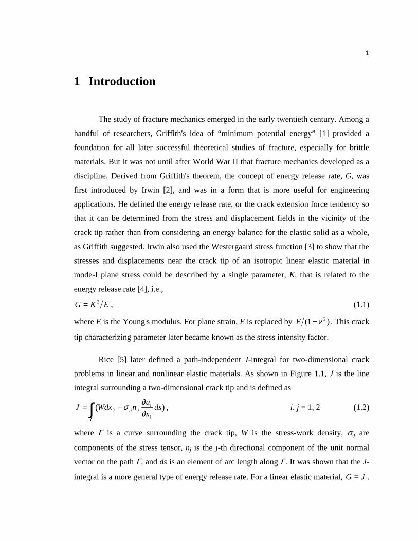
Rice [5] later defined a path-independent J-integral for two-dimensional crack
problems in linear and nonlinear elastic materials. As shown in Figure 1.1, J is the line
integral surrounding a two-dimensional crack tip and is defined as
∫ ∂∂−= i
jij dsx
unWdxJ )(
12 σ , i, j = 1, 2 (1.2)
where Γ is a curve surrounding the crack tip, W is the stress-work density, σij are
components of the stress tensor, nj is the j-th directional component of the unit normal
vector on the path Γ, and ds is an element of arc length along Γ. It was shown that the J-
integral is a more general type of energy release rate. For a linear elastic material, JG = .

2
Therefore, the stress intensity factor K can be readily obtained, according to Eq.(1.1) and
the computational efficiency of the J-integral, as
JEK = . (1.3)
The J-integral is effective for evaluating K in two-dimensional crack problems.
For three-dimensional problems, however, it is difficult to distinguish K at different x3
locations, assuming the line integral is performed on the x1-x2 plane. Thus an alternative
procedure needs to be developed to determine the distribution of K through the thickness.
Parks [6] employed the virtual crack extension method to determine J from elastic-plastic
finite element solutions. The method is based on an energy comparison of two slightly
different crack lengths and requires only one elastic-plastic finite element solution,
because the altered crack configuration is obtained by changing nodal positions. The
procedure is directly applicable to two-dimensional configurations but can be extended in
a straightforward manner to obtain arc-length-weighted average values of J along three-
dimensional crack fronts. The three-dimensional applications, however, have significant
loss of accuracy in the near-tip region where the values of field quantities (stresses,
strains, and displacements) are required to determine the point-wise energy release rate
along the crack front. Based on the virtual crack extension method, deLorenzi [7,8]
developed a finite element method that is more general to calculate the energy release
rate in two-dimensional and three-dimensional fracture problems and could include the
effects of body forces and traction loading on the crack faces.
Another investigation was made by Li et al. [9]. They proposed a formulation
which would convert area integrals to volume integrals in order to calculate point-wise
values of the energy release rate along a three-dimensional crack front. Shih, Nakamura
and co-workers [10,11] then developed a finite element formulation to calculate the
volume domain integral. About the same time, Nikishkov and Atluri [12,13] applied a
somewhat different approach but a similar numerical procedure, and named the
formulation “equivalent domain integral (EDI)” which would be used by subsequent
researchers [14-16]. All of those derivations involve the application of the divergence

3
theorem and the implementation of a spatial weighting function that is based upon the
virtual crack extension method.
With the EDI method, a point-wise value of J along a three-dimensional crack
front can be calculated, and therefore the value of K along the crack front can be obtained
from Eq.(1.3). Another advantage is that the EDI method transforms surface integrals in a
three-dimensional problem into integrals over a volume, or a domain (hence the name of
equivalent domain integral), without evaluation of the stress singularities directly on the
crack front.
The stress intensity factor alone is not enough to characterize the crack behavior
in some cases. Other fracture parameters may be needed to describe the crack behavior
more precisely. As Irwin [4] pointed out there is a mathematical expression for crack-tip
stress distributions in linear isotropic solids, Williams [22] showed that the expression is
in fact an infinite power series of r, where r is the distance from the crack tip. The power
series, in a concise form, can be written as
∑∞
−=
=1
)()2/1( )(),(n
nij
nnij frAr θθσ , i, j = 1, 2 (1.4)
where An are unknown constants which depend on the geometry and loading conditions,
and )()( θnijf are the known angular distributions. The mode-I stress intensity factor is
included in the first term of Eq.(1.4) as
)(2
lim )1(I
0θ
πσ −
→= ij
rij f
r
K, (1.5)
in which the stresses are singular at 0=r and π2I1 KA = . The leading term of the
series of Eq.(1.4) represents r-1/2 singularity; the second term is a constant; the third and
higher-order terms are proportional to r(1/2)n, n=1,2,3…. Larsson and Carlsson [23] first
denoted this constant term as T, and later it became the so-called “elastic T-stress”.
In addition to the stress intensity factor, the elastic T-stress provides another
parameter to identify the severity of stress and displacement fields near a crack. Larsson

4
and Carlsson [23] showed that the T-stress is necessary to modify the solution of the
stress state in a small-scale yielding crack problem in plane strain condition. Rice [24]
showed that T is in fact a constant stress parallel to the crack flank, and included it as a
second crack tip parameter to characterize suitably small plane strain yield zones. Several
methods have been used to practically determine the T-stress [25]. In addition to the
methods mentioned in [25], recently other methods were also used, such as the boundary
layer method and the displacement field method [26], as well as the stress difference
method [27]. Among those methods, the interaction integral method developed by
Nakamura and Parks [28] demonstrated highly computational effectiveness since it is
based on the EDI method and has the capability to compute the T-stress not only in an
isotropic material but also in an anisotropic material.
Under the NASA Advanced Composite Technology Program, Langley Research
Center (LaRC) has performed fracture toughness tests for various types of wing structure
specimens made from stitched warp-knit fabric composites. Variations of in-plane
geometry and crack length were evaluated from three kinds of specimen geometry [29]:
compact tension (CT) specimen with the crack aspect ratios 69.046.0 ≤≤ wa ; center-
cracked tension (CCT) specimen with 42.0226.0 ≤≤ wa ; single-edge notched tension
(SENT) with 34.025.0 ≤≤ wa .
Methods based on the equivalent domain integral and Betti’s reciprocal theorem
were developed by Yuan and Yang [29] to extract the fracture parameters – critical stress
intensity factor and T-stress. With the limited experimental data, the results tend to show
that the critical mode-I stress intensity factor provides a satisfactory characterization for
engineering applications of fracture initiation in the composite of a given laminate
thickness, provided the failure is fiber-dominated and the crack growth follows in a self-
similar manner. In addition, the high constraint due to high tensile T-stress may be
expected to inhibit the crack extension in the same plane and promote the crack turning.
Recently, LaRC performed a mode-I test on a five-stringer panel manufactured

5
using the stitched warp-knit composite material. The crack initially extended in a self-
similar manner and then turned parallel to the stiffener direction when the crack
approached stiffeners (see Figure 1.2). In this dissertation, the effects of the geometrical
attributes on the fracture behavior of this panel are investigated by using three-
dimensional finite element analysis and linear elastic fracture mechanics to analyze the
composites. Due to the high computational efficiency, the equivalent domain integral
method is used to calculate the through-thickness KI stress intensity factor and the
interaction integral method is adopted to compute the through-thickness T-stress
components. The algorithms of the equivalent domain integral and interaction integral are
implemented into a single computer program, which reads a set of finite element
solutions from a given mesh as the input to determine the distributions of the fracture
parameters along the crack front. The composites are modeled as linear, anisotropic, and
homogeneous materials. For the purpose of verification and comparison, a similarly
cracked plate structure without stiffeners is also analyzed with the same composite
material properties as well as an isotropic material.
The derivation of the EDI method is reviewed in Chapter 2 by the approaches
mostly found in [15]. The derivation of the auxiliary fields necessary in the interaction
integral method for an anisotropic material is presented in Chapter 3. Chapter 4 shows the
procedure to determine the stress intensity factor and components of the T-stress from the
values of the equivalent domain integral and interaction integral. The finite element
models used in this research are described in Chapter 5; the associated results are
presented in Chapter 6. Finally, the summary and discussion is presented and suggestions
for future research are made in Chapter 7.

6
Figure 1.1 An arbitrary path on which a line integral is to be calculated.
θr
x1
x2
Γ
ds

7
Fig
ure
1.2
The
cra
cked
sti
ffen
ed p
anel
to b
e an
alyz
ed in
the
diss
erta
tion
. (C
ourt
esy
of N
ASA
Lan
gley
Res
earc
h C
ente
r)

8
2 Equivalent Domain Integral (EDI)
The derivation will assume a traction-free crack in a linear elastic material, with
the intention of determining the mode-I stress intensity factor KI through the thickness.
2.1 Mathematical Formulation
Let us consider a small cylindrical volume with radius ε encompassing a segment
of crack front of length ∆ such that both ε and ∆ approach zero, as shown in Figure 2.1. A
local coordinate system is defined so that the axes x1 and x2 are perpendicular to the crack
front, while x1 and x3 are lying on the crack plane. The volume is enclosed by five areas,
namely the outer surface Aε, two end surfaces Aε1 and Aε2, the top crack surface Aεct, and
the bottom crack surface Aεcb.
The local J-integral over the outer surface Aε of the tube is defined as [30]
dAnx
uWnJ j
iij∫ ∂
∂−∆
=→→∆
)(1
lim1
1
00
σε
. i, j = 1, 2, 3 (2.1)
In Eq.(2.1), W is the stress-work density, defined as ∫= ijijdW εσ , where σij are
components of the stress tensor, and εij are components of the strain tensor. ui are
components of the displacement vector; nj is the j-th directional component of the unit
normal vector on the surface Aε. Since this research will be limited only to linear elastic
materials, the stress-work density is simplified as 2)( ijijW εσ= . Note that
displacements, strains, stresses are expressed in the local crack front coordinate system.
For the purpose of simplicity in later derivations, let
ji
ij nx
uWnQ
11 ∂
∂−= σ . (2.2)
Then Eq.(2.2) can be rewritten in terms of boundaries shown in Figure 2.1 to complete a

9
surface integral as
++
∆= ∫∫∫
++→→∆
cbct AAAAA
QdAQdAQdAJεεεεεε 21
1lim
00
. (2.3)
The evaluation of surface integrals in Eq.(2.3) is tedious and could lead to errors because
singular terms on the crack front are included for numerical integration. Therefore, a
modified form of the surface integrals is desirable, and this modified form would be the
equivalent domain integral.
Now consider two tubular surfaces, A and Aε , as shown in Figure 2.2. A is an
arbitrary surface enclosing Aε on which the J-integral is calculated. A1 and A2 are end
surfaces connecting A and Aε . (A-Aε)ct and (Aε-A)cb denote the top and bottom crack
surfaces between A and Aε, respectively. An enclosed volume (V-Vε) is surrounded by all
of these surfaces, which are called collectively AΣ, defined as
21)()( AAAAAAAAA cbct ++−+−+−=Σ εεε . (2.4)
Based on the virtual crack extension theory, deLorenzi [8] proposed the concept
of virtual node shift that forms the definition of a spatial weighting function, which is
called s-function by some researchers [12-16,30]. We will adopt this name throughout
this dissertation and use the symbol s to represent this spatial weighting function.
According to the configuration shown in Figure 2.2, an arbitrary but continuous s-
function is defined between A and Aε so that the function has the following properties:
0),,( 321 =xxxs on A, Aε1 and Aε2, A1 and A2; (2.5a)
)(),,( 3321 xsxxxs = on Aε. (2.5b)
In order to complete the surface integrals over AΣ, the first integral in Eq.(2.3) can
be rewritten as an integral over the closed surface AΣ and an integral over the physical
boundaries cbct AAAA )()( −+− εε . And with the use of Eq.(2.5), Eq.(2.3) becomes

10
+++−= ∫∫∫∫
++−+−Σ cbctcbct AAAAAAAAA
QsdAQdAQsdAQsdAf
Jεεεεεε 21)()(
1. (2.6)
In Eq.(2.6) f is the area under the s-function curve on surface Aε and is defined as
∫∆
= 33 )( dxxsf . (2.7)
The s-function is equal to zero on both end surfaces of Aε1 and Aε2; therefore,
021
=∫+ εε AA
QsdA and Eq.(2.6) remains as
++−= ∫∫∫
+−+−Σ cbctcbct AAAAAAA
QsdAQsdAQsdAf
Jεεεε )()(
1. (2.8)
In Eq.(2.8) the negative sign of the first integral, which is over an enclosed
domain, comes from the opposite direction of the outer normal vector to the surface Aε of
the volume (V-Vε) in comparison with the normal vector to the surface Aε in Figure 2.1.
The other integrals in Eq.(2.8) are actually on the crack surfaces. Therefore, we may
separate integrals in Eq.(2.8) into a “domain” integral and a “crack face” integral,
denoted as
[ ]facecrack domain )()(1
JJf
J += , (2.9)
where ∫Σ
−=A
QsdAJ domain)( , (2.10)
and ∫∫∫ =+=+−+−
sdAQQsdAQsdAJ
cbctcbct AAAAAA
facecrack
)()(
facecrack )(εεεε
. (2.11)
By recalling Eq.(2.2), Eq.(2.10) can be written as
∫Σ
∂∂−−=
A
ji
ij dAnsx
uWsnJ
11domain)( σ . (2.12)
The use of divergence theorem on Eq.(2.12) gives the following result:

11
sdVxx
WdV
x
s
x
u
x
sWJ
VV
ijij
VV j
iij ∫∫
−−
∂∂
−∂∂−
∂∂
∂∂−
∂∂−=
εε
εσσ
1111domain)( . (2.13)
Since the analysis is limited to linear elastic materials, it can be shown that the second
integral in Eq.(2.13) is equal to zero [13]. Thus Eq.(2.13) is simplified as
dVx
s
x
u
x
sWJ
VV j
iij∫
−
∂∂
∂∂−
∂∂−=
ε
σ11
domain)( . (2.14)
On the crack surfaces, the first and third directional components of the unit
normal vector n are equal to zero ( 031 == nn ), according to the local coordinate system.
The second component of n has the properties of 12 +=n on the bottom face and
12 −=n on the top face. Upon substituting these conditions into Eq.(2.2), we have
∂∂+
∂∂+
∂∂−= 2
1
3322
1
2222
1
1121facecrack n
x
un
x
un
x
uWnQ σσσ . (2.15)
Since 03222 == σσ on the crack surfaces, Eq.(2.15) is then reduced to
21
112facecrack n
x
uQ
∂∂−= σ . (2.16)
For a traction-free crack surface, 012 =σ . Thus the value of Q in Eq.(2.16) is equal to
zero, and all integrals in Eq.(2.11) vanish.
Therefore, for a traction-free crack in a linear elastic material, the equivalent
domain integral for the determination of KI, in terms of displacements, strains, and
stresses, can be conveniently expressed as
dVx
s
x
u
x
sW
fJ
V j
iij∫
∂∂
∂∂−
∂∂−=
111
1 σ . (2.17)
To make a computable expression of Eq.(2.17), some numerical implementation needs to
be defined.
12
2.2 Numerical Implementation
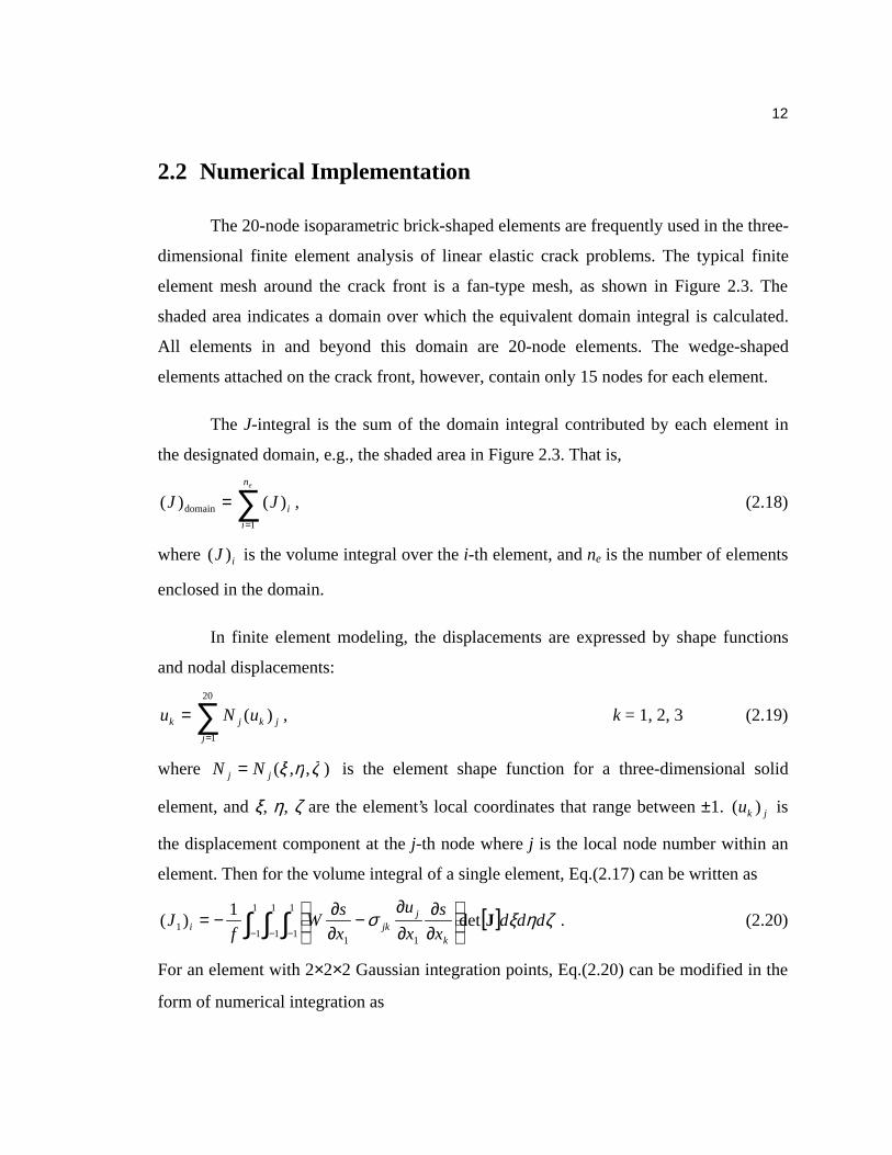
The 20-node isoparametric brick-shaped elements are frequently used in the three-
dimensional finite element analysis of linear elastic crack problems. The typical finite
element mesh around the crack front is a fan-type mesh, as shown in Figure 2.3. The
shaded area indicates a domain over which the equivalent domain integral is calculated.
All elements in and beyond this domain are 20-node elements. The wedge-shaped
elements attached on the crack front, however, contain only 15 nodes for each element.
The J-integral is the sum of the domain integral contributed by each element in
the designated domain, e.g., the shaded area in Figure 2.3. That is,
∑=
=en
i
iJJ1
domain )()( , (2.18)
where iJ )( is the volume integral over the i-th element, and ne is the number of elements
enclosed in the domain.
In finite element modeling, the displacements are expressed by shape functions
and nodal displacements:
∑=
=20
1
)(j
jkjk uNu , k = 1, 2, 3 (2.19)
where ),,( ζηξjj NN = is the element shape function for a three-dimensional solid
element, and ξ, η, ζ are the element’s local coordinates that range between ±1. jku )( is
the displacement component at the j-th node where j is the local node number within an
element. Then for the volume integral of a single element, Eq.(2.17) can be written as
[ ] ζηξσ dddx
s
x
u
x
sW
fJ
k
jjki Jdet
1)(
1
1
1
1
1
111
1 ∫ ∫ ∫− − −
∂∂
∂∂
−∂∂−= . (2.20)
For an element with 2×2×2 Gaussian integration points, Eq.(2.20) can be modified in the
form of numerical integration as

13
[ ]im n p
pnmxi wwwx
sW
fJ
′′−∂∂−= ∑∑∑
= = =
Jsu det1
)(2
1
2
1
2
1
T
11 1
. (2.21)
In Eq.(2.21), W is the stress-work density, T
1xu ′ is the vector of displacement derivatives,
σ is the stress tensor, s’ is the derivatives of the s-function, and det[J] denotes the
determinant of the Jacobian matrix. wm, wn, and wp are integration weights, and they all
have the values of unity for 2×2×2 reduced integration [31].
Eq.(2.21) is the equation to be used for computation; therefore, the numerical
implementation of each item in this equation needs to be explicitly expressed, as shown
in the following sections. Once all items in Eq.(2.21) can be readily calculated, the J-
integral over the domain can be evaluated from Eq.(2.18).
2.2.1 The Jacobian Matrix
The Jacobian matrix is defined by
∂∂
∂∂
∂∂
∂∂
∂∂
∂∂
∂∂
∂∂
∂∂
=
ζζζ
ηηη
ξξξ
321
321
321
xxx
xxx
xxx
J . (2.22)
Each component of the matrix, according to the finite element theory, is defined as
∑=
∂∂
=∂∂ 20
1
)(j
jkjk x
Nx
ξξ, k = 1, 2, 3 (2.23a)
∑=
∂∂
=∂∂ 20
1
)(j
jkjk x
Nx
ηη, k = 1, 2, 3 (2.23b)
∑=
∂∂
=∂∂ 20
1
)(j
jkjk x
Nx
ζζ, k = 1, 2, 3 (2.23c)
where jkx )( is the local coordinate component at the j-th node within an element.

14
2.2.2 The Stress Tensor and Stress-Work Density
The stress tensor σ of a linear elastic material is a 3×3 symmetric matrix shown as
=
332313
232212
131211
σσσσσσσσσ
. (2.24)
The stress-work density of the linear elastic material is 2)( ijijεσ , or
( ) 1313232312123333222211112
1 εσεσεσεσεσεσ +++++=W . (2.25)
Note that σij and εij are the stress and strain components from the finite element solutions
output on the integration points.
2.2.3 The Derivatives of the s-Function
s’ is the vector containing derivatives of the s-function with respect to the local
coordinate system and is expressed as
T
321
∂∂
∂∂
∂∂=′
x
s
x
s
x
ss . (2.26)
To evaluate Eq.(2.26), the s-function must be defined first. Since the s-function is
arbitrary and satisfies Eq.(2.5), it can be conveniently defined by the sums of the element
shape functions as
∑=
=20
1
),,(j
jj sNs ζηξ . (2.27)
For the 20-node brick-shaped element shown in Figure 2.4, the s-function is
completely defined by specifying 1)14()10( == ss and zero on all other nodes in order to
satisfy Eq.(2.5). This definition yields a quadratic s-function over a single element. With
the definition, Eq.(2.7) also can be evaluated and hence f = (2/3)∆ where ∆ is the length
of the domain segment [30].

15
It is clear that the s-function is a function of the element coordinate system (ξ, η,
ζ), rather than the crack front coordinate system (x1, x2, x3). Thus s’ should be expressed
in terms of (ξ, η, ζ) before it can be evaluated. This can be done by the chain rule, as
shown in the following equation:
∂∂∂∂∂∂
=
∂∂
∂∂+
∂∂
∂∂+
∂∂
∂∂
∂∂
∂∂+
∂∂
∂∂+
∂∂
∂∂
∂∂
∂∂+
∂∂
∂∂+
∂∂
∂∂
=
∂∂∂∂∂∂
=′ −
ζ
η
ξ
ζζ
ηη
ξξ
ζζ
ηη
ξξ
ζζ
ηη
ξξ
s
s
s
x
s
x
s
x
sx
s
x
s
x
sx
s
x
s
x
s
x
sx
sx
s
1
333
222
111
3
2
1
Js . (2.28)
J-1 is the inverse Jacobian matrix containing the following components:
333
222
111
1
∂∂
∂∂
∂∂
∂∂
∂∂
∂∂
∂∂
∂∂
∂∂
=−
xxx
xxx
xxx
ζηξ
ζηξ
ζηξ
J . (2.29)
The derivatives of the s-function with respect to the element coordinate system, i.e. ξ∂
∂s,
η∂∂s
and ζ∂
∂s in Eq.(2.28), can be evaluated in the same manner as Eq.(2.23).
2.2.4 The Derivatives of the Displacements
T
1xu ′ is the vector of displacement derivatives and can be expressed as
∂∂
∂∂
∂∂=′
1
3
1
2
1
1T
1 x
u
x
u
x
uxu . (2.30)
The components in Eq.(2.30) are the derivatives of the displacements with respect to the
local coordinate system. Similar to the derivatives of the s-function, they should be
evaluated in terms of the element coordinate system (ξ, η, ζ). With the use of the chain
rule on Eq.(2.19), each component of Eq.(2.30) can be obtained by
16
( )jk
j
jjjk ux
N
x
N
x
N
x
u ∑=
∂∂
∂∂
+∂∂
∂∂
+∂∂
∂∂
=∂∂ 20
1 1111
ζζ
ηη
ξξ
. k = 1, 2, 3 (2.31)
In Eq.(2.31), 1x∂
∂ξ,
1x∂∂η
and 1x∂
∂ζ are the components of the first row of the inverse
Jacobian matrix of Eq.(2.29); ξ∂
∂ jN,
η∂∂ jN
and ζ∂
∂ jN are the derivatives of the shape
functions that can be readily computed.

17
Figure 2.1 A small cylindrical volume around a segment of crack front, with the localcoordinate system shown.
Figure 2.2 A domain enclosing a segment of crack front.
x1
x2
x3
ε∆
Aε
Aεct
Aε2
Aεcb
Aε1
crack front
ε∆
s-function
x1
x2
x3
Aε
A1
A
A2
V-Vε
(Aε-A)cb(A-Aε)ct

18
Figure 2.3 The schematic finite element mesh near a segment of the crack front.
Figure 2.4 A 20-node element with the associated s-functions.
x1
x3
x2
x1
x2
x3
∆
2
3
5
6
7
8
410
11
13
14 15
16
20
19
18
19 12
17
crack front

19
3 Interaction Integral
The interaction integral is necessary for extracting the elastic T-stress from an
existing finite element solution. It is based upon the formulation of the EDI method as
well as a superimposed auxiliary stress field. Kfouri [32] gave the auxiliary stress field
that is the analytical solution corresponding to a point force applied to a crack tip and
parallel to the crack surface under plane strain in isotropic solids. For a three-dimensional
crack, the point force becomes a uniform line load that is applied along the crack front, as
shown in Figure 3.1(a). This stress field is a function of r, the distance from the crack
front, and θ, the angle from x1 axis toward x2 axis; but it is independent of the crack front
location x3.
Nakamura and Parks [28] applied the auxiliary stress field with the interaction
integral and successfully calculated the T-stress distribution along the three-dimensional
crack front. The auxiliary stress field, however, is valid only for isotropic materials. For
anisotropic materials, the corresponding auxiliary fields have been derived using Stroh
formalism [34].
Similar to Eq.(2.17) of the equivalent domain integral, the interaction integral for
mode-I loading in a given domain may be expressed as
dVx
s
x
u
x
u
x
s
fI
V j
iij
iijijij∫
∂∂
∂∂+
∂∂+
∂∂−=
1
a
1
a
1
a1
1 σσεσ , i, j = 1, 2, 3 (3.1)
where aijσ , a
ijε , and aiu are the components of the auxiliary stress, strain, and
displacement fields, respectively. For the purpose of numerical integration of each
individual element in a domain, Eq.(3.1) can be written similarly to Eq.(2.21) as
( ) [ ]im n p
pnmxxjkjki wwwx
s
fI
′′+′+∂∂−= ∑∑∑
= = =
Jsuu det)(1
)(2
1
2
1
2
1
aTTa
1
a1 11
εσ . (3.2)
In Eq.(3.2), σa and ua denote the stress tensor and displacement vector of the auxiliary

20
fields, respectively. ajkε are components of the auxiliary strain tensor. These entities are
expressed in terms of the components of the associated tensor or vector as follows:
=
a33
a23
a13
a23
a22
a12
a13
a12
a11
a
σσσσσσσσσ
; (3.3)
( )a1313
a2323
a1212
a3333
a2222
a1111
a 2 εσεσεσεσεσεσεσ +++++=jkjk ; (3.4)
∂∂
∂∂
∂∂=′
1
a3
1
a2
1
a1Ta
1)(
x
u
x
u
x
uxu . (3.5)
Quantities of Eq.(3.3) and Eq.(3.4) can be obtained by straightforward
substitution of auxiliary stress and strain fields. Components in Eq.(3.5) can be computed
similarly to Eq.(2.31) as
( )jk
j
jjjk ux
N
x
N
x
N
x
u a20
1 1111
a
∑=
∂∂
∂∂
+∂∂
∂∂
+∂∂
∂∂
=∂∂ ζ
ζη
ηξ
ξ, k = 1, 2, 3 (3.6)
where aku are components of the auxiliary displacement vector. All of the other items not
associated with the auxiliary fields are calculated exactly in the same way as the
equivalent domain integral is.
Since the auxiliary strain and displacement fields are derived from the auxiliary
stress field which is a function of r and θ, both are functions of r and θ as well. All terms
in Eq.(3.2), however, should be evaluated with respect to the local coordinates (x1, x2, x3).
Therefore, the auxiliary field calculation must be done by converting the Cartesian
coordinates of nodes or integration points to the polar coordinates before substituting
them into the auxiliary field formulation. The computation of the auxiliary displacement
field is straightforward because it needs only substitution of all 20 nodes’ coordinates
within an element. The auxiliary stresses and strains will need the coordinates of the 8
integration points. The location of these integration points with respect to the element
coordinate system is illustrated in Figure 3.2.

21
Let us recall the Williams expansion of Eq.(1.4) which can be generalized to
three-dimensional problems. It is assumed that the asymptotic expansion of the stress
field near the crack front location under general loading conditions can be expressed as
)1()(2
III)(3
I)(1
)( oTfr
kij
n
nij
nij ++= ∑
=
θπ
σ , i, j = 1, 2, 3 (3.7)
where kI, kII, and kIII are local stress intensity factors, )()( θnijf are angular distributions for
the crack-tip field given by the two-dimensional deformation of anisotropic elasticity
theory, and o(1) represents other higher order terms. Tij are the non-singular T-stresses,
which have three distinct components, namely
[ ]
=
3313
1311
0000
0
TT
TTTij . (3.8)
T11 is obviously the stress component acting parallel to the crack plane [24] and
can be determined by the interaction integral with an imposed uniform line load f1 as
shown in Figure 3.1(a). Similarly T13 can be determined by using a different set of
auxiliary fields. Instead of the line load perpendicular to the crack front and the x2-x3
plane, a constant force f3 in x3-direction and through the full length of crack front should
be imposed. This configuration, as shown in Figure 3.1(b), will yield an auxiliary stress
field necessary to extract T13. T33 is a combination of T11 and T13 and can be readily
obtained after the other two T-stresses are determined (see Chapter 4).
In the following sections, the derivations of both types of auxiliary fields are
presented in order to determine all of the T-stress components.
3.1 Auxiliary Fields for T11
In this dissertation, we will be concerned with the composite plate structures,
which usually have at least one plane of symmetry in materials. The convention of
orientation for a composite plate is that the plate is on the x1-x2 plane while the x3 is the

22
direction out of plane [34]. Since most composite plates have at least one symmetry plane
at x3=0, we will limit the derivation under this restriction. This kind of material is called
the monoclinic material with the plane of symmetry at x3=0, or simply the monoclinic
material about x3=0.
The generalized Hooke’s law states the stress-strain relation in contracted notation
as
cc C= , (3.9)
where [ ] [ ]T121323332211
T654321
c σσσσσσσσσσσσ == (3.10)
and [ ] [ ]T121323332211
T654321
c 222 εεεεεεεεεεεε == . (3.11)
C is a 6×6 matrix, and is called the stiffness matrix in which the components Cij are
material properties. A monoclinic material about x3=0 has the following form of the
stiffness matrix:
=
66362616
5545
4544
36332313
26232212
16131211
0000000000
000000
CCCCCCCC
CCCCCCCCCCCC
C . (3.12)
The inverse of the stress-strain relation defines the compliance matrix s, as
cc s= , (3.13)
where s is the inverse of C. Thus the compliance matrix of a monoclinic material about
x3=0 has the form of
== −
66362616
5545
4544
36332313
26232212
16131211
1
0000000000
000000
ssssssss
ssssssssssss
Cs . (3.14)
As stated earlier, the auxiliary fields for T11 are independent of x3. This implies it
is under the condition of two-dimensional deformation for which ε3=0. By ignoring the

23
equation for σ3 in Eq.(3.9), the stress-strain relation of the monoclinic material can be
written as
[ ] [ ]T54621
0T54621 εεεεεσσσσσ C= , (3.15)
where C0 is the reduced stiffness matrix, shown as
=
5545
4544
662616
262212
161211
0
000000
000000
CCCC
CCCCCCCCC
C . (3.16)
The inverse of Eq.(3.16) gives the definition of the reduced compliance matrix s0, as
( )
′′′′
′′′′′′′′′
== −
5545
4544
662616
262212
161211
100
000000
000000
ssss
sssssssss
Cs . (3.17)
The components of s0 can be also obtained by solving for σ3 in the third equation
of Eq.(3.13) that will yield
∑=
−==6
1
333
333
1
βββσσσ s
s. 3≠β (3.18)
Substituting Eq.(3.18) into the other five equations of Eq.(3.13) will have
33
33
s
ssss ji
ijij −=′ . i, j = 1, 2, 4, 5, 6 (3.19)
According to Stroh formalism for two-dimensional deformations of an anisotropic
elastic body [35], the characteristic equations have the reduced compliance as
coefficients:
02)2(2 22262
66123
164
11 =′+′−′+′+′−′ ssssss µµµµ ; (3.20a)
02 44452
55 =′+′−′ sss µµ . (3.20b)
The solutions to Eq.(3.20) are the eigenvalues of elastic constants, µα (α = 1, 2, 3), where
µ1, µ2, 1µ , and 2µ are roots of Eq.(3.20a), and µ3, 3µ are roots of Eq.(3.20b). µα are

24
complex numbers, and αµ are the conjugates of µα.
Under the uniform line load f1 shown in Figure 3.1(a), the auxiliary stresses are
inversely proportion to r, or 1a −∝ rijσ . In Stroh formalism, the real form solution for the
displacement ua and the stress function φa due to the point forces can be written as
fLSIu 1a )(ln
2 −
+−= θ
πr
, (3.21a)
fLL 1a )(=2 −θφ , (3.21b)
where S and L are Barnette-Lothe tensors, S(θ) and L(θ) are their associate tensors, f is
the vector of the line load per unit thickness, and I is the 3×3 identity matrix. These items
are defined as follows:
T1 ]00[ f=f ; (3.22)
( ) TsincoslnRe2
)( BAS θµθπ
θ α+= ; (3.23a)
( ) TsincoslnRe2
)( BBL θµθπ
θ α+−= ; (3.23b)
( )
′′=
−
−
111
2
21
111
0000
smezzz
sL . (3.24)
The definitions of the terms in Eq.(3.23) and Eq.(3.24) are given as follows.
For the purpose of simplicity, let θµθς αα sincos += . In Eq.(3.23), implies a
diagonal matrix, thus
( )
=+
3
2
1
ln000ln000ln
sincoslnς
ςς
θµθ α . (3.25)
A and B are 3×3 complex matrices containing Stroh eigenvectors and are defined as

25
′−′=
)(0000
344453
2211
2211
µsskqkqkpkpk
A and (3.26a)
−
−−=
3
21
2211
0000
kkkkk µµ
B , (3.26b)
where p1, p2, q1, q2 can be obtained from
12162
11 sssp ′+′−′= ααα µµ and ααα µµ 222612 sssq ′+′−′= . α = 1, 2 (3.27)
k1, k2, k3 are normalization factors satisfying the following relations:
1)(2 11121 =− pqk µ ; 1)(2 222
22 =− pqk µ ; 1)(2 45344
23 =′−′ ssk µ . (3.28)
The components of L-1 in Eq.(3.24) are defined by the following relations:
izy 1121 +=+ µµ ; (3.29a)
izy 2221 +=µµ ; (3.29b)
1221 zyzye −= ; (3.29c)
( ) 2/145455544
−′′−′′= ssssm . (3.29d)
Upon substitution of Eq.(3.22) through Eq.(3.24), the stress function of
Eq.(3.21b) can be obtained as
′
−=0
Re 2
1111a φ
φ
πsfφ , (3.30)
where ( ) ( )222211
2122
22
221
21
2111 lnlnlnln ςµςµςµςµφ kkzkkz +−+= (3.31a)
and ( ) ( )2221
21222
2211
2112 lnlnlnln ςςςµςµφ kkzkkz +++−= . (3.31b)
To determine the auxiliary stress field from the stress function, let tr be the
traction vector on a cylindrical surface of r = constant which can be obtained as [33]
θφ
∂∂−=
rr
1t , (3.32)

26
or
′
=0
Re2
1111
r
r
r tt
r
sf
πt , (3.33)
where ( ) ( )222211
2122
22
221
21
2111
Ω+Ω−Ω+Ω= µµµµ kkzkkztr (3.34a)
and ( ) ( )2221
21222
2211
2112
Ω+Ω+Ω+Ω−= kkzkkztr µµ . (3.34b)
In Eq.(3.34) Ωα is defined as
θµθθµθς
θθ
α
ααα sincos
cossinln)(
++−=
∂∂=Ω . α = 1, 2, 3 (3.35)
Then the stresses in the cylindrical coordinate system are
[ ] rrr t0sincos θθσ = ; (3.36a)
[ ] rr t1003 =σ ; (3.36b)
03 === θθθθ σσσ r . (3.36c)
σr3 is found to be equal to zero after substituting Eq.(3.33) into Eq.(3.36b). Substitution
of Eq.(3.33) into Eq.(3.36a) also gives σrr, which is a function of r and θ, as
θθπ
σ sincosRe21
111rrrr tt
r
sf +′
= . (3.37)
It should be noted that the auxiliary fields in the calculation of the interaction
integral of Eq.(3.1) are all in the Cartesian coordinate system. Hence the auxiliary
stresses aijσ must be obtained by applying coordinate transformation on Eq.(3.36). The
results, which will be able to be implemented into the numerical computing procedure,
are given as follows:
θθπ
θσ sincosRecos
21
2111a
11 rr ttr
sf +′
= ; (3.38a)
θθπ
θσ sincosResin
21
2111a
22 rr ttr
sf +′
= ; (3.38b)
θθπ
θθσ sincosRecossin
21
111a12 rr tt
r
sf +′
= ; (3.38c)
0a23
a13 == σσ . (3.38d)

27
a33σ can be obtained by substitution of Eq.(3.38) into Eq.(3.18), which yields
( ) θθπ
θθσ sincosResincos
21
33
223
213111a
33 rr ttrs
sssf ++′−= . (3.38e)
Once the auxiliary stress field is available, the auxiliary strain field can be readily
obtained from the inverse of the stress-strain relation of Eq.(3.13).
The auxiliary displacement field is readily available from Eq.(3.21a) which, after
a series of substitution of Eq.(3.22) through Eq.(3.24), will yield 0a3 =u and non-zero
items of a1u and a
2u as
+++
′
−=
222211
122111
2
1111a2
a1 Re2ln
2 SzSzSzSz
rzzsf
uu
π, (3.39)
where S11, S21, S12, and S22 are components of S(θ) and are defined as
22222111
2111 lnln ςµςµ pkpkS −−= ; (3.40a)
222211
2112 lnln ςς pkpkS += ; (3.40b)
22222111
2121 lnln ςµςµ qkqkS −−= ; (3.40c)
222211
2122 lnln ςς qkqkS += . (3.40d)
Without loss of generality, the magnitude of the line load may be chosen as f1=1
as f is arbitrary. This assumption, as well as the information on material properties and
nodal coordinates, will enable the calculation of the auxiliary fields necessary for the
evaluation of the interaction integral, which in turn will determine T11.
The auxiliary stress field for T11 in an isotropic material was given by Nakamura
and Parks [28] as
θπ
σ 31a11 cos
r
f−= ; (3.41a)
θθπ
σ 21a22 sincos
r
f−= ; (3.41b)
28
θθπ
σ sincos21a12 r
f−= ; (3.41c)
θνπ
σ cos1a33 r
f−= ; (3.41d)
0a23
a13 == σσ . (3.41e)
It can be shown from strain-displacement relations that the auxiliary displacement field is
( )( )
−
+−−=νθ
πν
12
sinln
1 21
2a1 r
E
fu ; (3.42a)
( ) ( )[ ]θθθνπν
cossin212
1 1a2 −−+−=
E
fu ; (3.42b)
0a3 =u . (3.42c)
3.2 Auxiliary Fields for T13
The approach to determine the auxiliary fields for T13 is similar to that of T11,
except the line load f1 is replaced by a constant force f3 in the x3-direction, as shown in
Figure 3.1(b). This configuration will change the line load vector f in Eq.(3.22) as
T3 ]00[ f=f , (3.43)
which will yield a different stress function as
−=3
23
3a
ln00
Reςπ km
fφ . (3.44)
By applying a similar derivation following Eq.(3.32) and Eq.(3.36), the auxiliary stresses
in the polar coordinate system can be obtained as
323
33 Re Ω= k
mr
fr π
σ , (3.45a)
03 ==== rrr σσσσ θθθθ . (3.45b)
Note that Ω3 is obtained through the definition of Eq.(3.35).
The transformation of stresses from r-θ plane to x1-x2 plane gives the results that

29
a11σ , a
12σ , and a22σ all are equal to zero because 0=== θθθ σσσ rrr . The transformation
of σr3, and σθ3 is conducted by the following relation [36]:
−=
3
3
23
13
cossinsincos
θσσ
θθθθ
σσ r . (3.46)
This operation yields the non-zero auxiliary stress components
323
3a13 Re
cos Ω= kmr
f
πθσ , (3.47a)
323
3a23 Re
sin Ω= kmr
f
πθσ . (3.47b)
Then a33σ can be obtained by the use of Eq.(3.18) that also shows 0a
33 =σ . This operation
assumes a monoclinic material about x3=0 by using its compliance components shown in
Eq.(3.14).
The auxiliary strain field is also readily obtained from the inverse of the stress-
strain relation of Eq.(3.13). And the auxiliary displacement field is available from
Eq.(3.21a) as well. But with a different f, both a1u and a
2u will be equal to zero while only
a3u is the non-zero displacement as
( )33a
3 lnReln2
ςπ
+−= rm
fu . (3.48)
The magnitude of the constant force may also be chosen as f3=1 because f is
arbitrary. Hence the auxiliary fields can be calculated, and therefore the T13 for a
monoclinic material about x3=0 will be determined.
For an isotropic material, the auxiliary fields may be obtained by applying the
material properties on the stiffness matrix of Eq.(3.12). A similar derivation will yield
r
f
πθσ
2
cos3a13 −= , (3.49a)
r
f
πθσ
2
sin3a23 −= , (3.49b)

30
0a12
a33
a22
a11 ==== σσσσ ; (3.49c)
( )r
E
fu ln
13a3 π
ν+−= . (3.50)

31
Figure 3.1 Auxiliary line load on a three-dimensional crack: (a) uniform forces f1
normal to crack front; (b) uniform forces f3 parallel to crack front.
Figure 3.2 Locations of the integration points inside an element.
x2
x3
x1
x1
x3
x2
uniform forces f1
crack front
θ
r
(a) (b)
uniform forces f3
crack front
θ
r
1
2
34
56
78
η
ξζ
ξ
ξ
η η
ζ
ζ
56
7 8
87
3 4 4 1
581
1
31
31

32
4 Stress Intensity Factor and T-Stress
The formulations regarding the equivalent domain integral and the interaction
integral are implemented into a FORTRAN computer program, which uses the finite
element solutions computed from another ANSYS program as the input. Once the
equivalent domain integral and the interaction integral are evaluated, the stress intensity
factor and T-stresses can be determined. In the following sections, formulation to
determine both parameters will be shown in terms of those integral quantities and
appropriate material properties. These formulations can be easily implemented into the
FORTRAN program as well. The full contents of the ANSYS and FORTRAN programs
are provided in the Appendices.
4.1 Stress Intensity Factor
For an anisotropic cracked solid, the energy release rate G is related to the stress
intensity factor through [29,33,37]
kLk 1T
2
1 −=G , (4.1)
where [ ]IIIIIIT kkk=k are stress intensity factors and L-1 is the inverse of one of the
Barnett-Lothe tensors as shown in Eq.(3.24). In elastic materials, the energy release rate
G is equal to the value of J-integral. For a pure mode-I crack in an elastic material, kII =
kIII = 0, and Eq.(4.1) will reduce to
)(2
)( 32I
1131 xk
esxJ
′= , (4.2)
where x3 is the crack front location defined in Section 2.1, and J1(x3) is value of the
equivalent domain integral, as defined in Eq.(2.17), on this location. Therefore the local
stress intensity factor kI(x3) can be determined as
es
xJxk
11
313I
)(2)(
′= . (4.3)

33
For an isotropic material, L-1 has the form of
( )
−
−=−
ν
ν
1
100
01000112 2
1
EL . (4.4)
The Eq.(4.3) will become
231
3I 1
)()(
ν−= xEJ
xk , (4.5)
which is the plane strain condition as shown in Eq.(1.3).
4.2 T-Stress
The T-stress, in general, includes three components, namely T11, T13 and T33, as
shown in Eq.(3.8). T11 and T13 should be determined from the evaluation of interaction
integrals, while T33 can be readily obtained after T11 and T13 are computed.
Let I(1) and I(2) be the values of interaction integral of Eq.(3.1) when the
superposed uniform load is f1 and f3, respectively. For an anisotropic material, it can be
shown that the following relation between T-Stress and interaction integral exists [37]:
−
=
′′′′
3
3)2(
33333
13
1
3)1(
13
11
5515
1511
)(
)()(
f
xI
xs
s
f
xI
TT
ssss
ε, (4.6)
where ε33(x3) is the crack front extension strain at a given crack front location x3. I(1)(x3)
and I(2)(x3) are the interaction integrals on the domain at x3 due to f1 and f3, respectively.
Then T11 and T13 at the same crack front location may be expressed as
−
′′′′=
−
3
3)2(
33333
13
1
3)1(
1
5515
1511
313
311
)(
)()(
)()(
f
xI
xs
s
f
xI
ssss
xTxT
ε. (4.7)
The extension strain ε33(x3) can be determined independently from finite element results.

34
For a monoclinic material about x3=0, 015 =′s . Since f1 and f3 are arbitrary, they
may be chosen as 131 == ff without loss of generality. Therefore for this kind of
material, at any given crack front location x3, T11 and T13 can be determined solely by I(1)
and I(2), respectively. Eq.(4.7) then can be de-coupled as
−
′= )()(
1)( 333
33
133
)1(
11311 x
s
sxI
sxT ε ; (4.8a)
55
3)2(
313
)()(
s
xIxT
′= . (4.8b)
In modeling three-dimensional cracks along a given location x3, the T33
component is also induced by the extension strain ε33(x3) along the crack front. Thus T33
can be evaluated as [37]
[ ])()(1
)( 1335111333333
333 TsTsxs
xT +−= ε . (4.8c)
For isotropic materials,
Es
ν−=13 , E
s1
33 = , 035 =s ; E
s2
11
1 ν−=′ , ( )
Es
ν+=′ 1255 . (4.9)
Then Eq.(4.8) reduces to
[ ])()(1
)( 3333)1(
2311 xxIE
xT νεν
+−
= ; (4.10a)
( ) )(12
)( 3)2(
313 xIE
xTν+
= ; (4.10b)
)()()( 311333333 xTxExT νε += . (4.10c)
Note that Eq.(4.10a) and Eq.(4.10c) have been derived by Nakamura and Parks [28].

35
5 Models
5.1 Plates
Due to loading and geometry symmetry, one-eighth of a through-thickness center-
cracked plate is modeled by finite elements. The entire plate, shown in Figure 5.1, has a
total length of in. 802 =l , a total width of in. 402 =w , and a total thickness of
in. 33.02 =t The origin of the global Cartesian coordinate system is located at the center
of the plate. The X-axis is parallel to the crack flank surfaces and the Y-axis is orthogonal
to X and to the crack flank. The Z-axis is normal to the X-Y plane. A uniform
displacement u∞ equivalent to a strain value of 0.1% is prescribed on the far ends at
lY ±= . For the finite element model, symmetric boundary conditions are imposed on the
planes of 0 =X , 0 =Y ( wXa ≤≤ ), and 0 =Z . The displacement loading is also applied
on the surface at lY = . A local coordinate system is defined on the crack front at the
centerline of thickness. The x1-axis is perpendicular to the crack front and coincident with
the global X-axis. The x2-axis is also normal to the crack front but parallel to the global Y-
axis, and the x3-axis lies on the crack front and is parallel to global Z-axis as well, as
shown in Figure 5.2.
The finite element model is generated and solved by ANSYS, a general-purpose
finite element code. A typical mesh of the finite element model is shown in Figure 5.3. It
includes large brick-shaped elements far away from the crack front and small fan-shaped
elements near the crack front. The elements attached on the crack front are 15-node
wedge-shaped elements. The radial size of these elements, e0, is always equal to or less
than 1% of the characteristic length lc, defined as ],,min[ tawalc −= , i.e. cle ×≤ 01.00 ,
as shown in Figure 5.4. Other than these wedge-shaped elements, the crack front region
consists of 12 rings, each of which contains 12 elements. The width of each ring
(equivalent to the radial element size) increases as the ring moves farther away from the

36
crack tip. The largest radial element size at Ring #12 is 26 times the smallest one at Ring
#1, and its outer radius is kept at 100 times of e0, as shown in Figure 5.5. The half
thickness is divided into 20 element layers, in which are 5 small layers near the free
surface, 8 large layers near the centerline, and 7 mid-size layers in between. The three
element sizes of each of these layers, in terms of the half thickness t, are 0.03t, 0.05t, and
0.0625t, respectively. Figure 5.6 shows the mesh refinement and element sizes near the
crack front and through the thickness. The overall mesh contains 5640 elements and
25183 nodes with 75549 degrees of freedom. This mesh result showed appropriate
convergence on the calculation of the fracture parameters.
5.2 Stiffened Panels
A stiffened panel based on the dimensions of the plate mentioned in Section 5.1
has five stiffeners attached longitudinally on one side of the plate. This structure is
designed by Boeing for the all-composite wing skin in a commercial aircraft [29]. A
center crack of length 2a cuts through the central stiffener and the panel. Figure 5.7
shows the configuration of the panel as well as the detail dimensions of the stiffener. Due
to the presence of stiffeners and geometry symmetry, one-fourth of the entire panel is
modeled by finite elements, as shown in Figure 5.8. Both of the global and local
Cartesian coordinate systems are defined in the same way they are defined in a plate.
Hence the symmetric boundary conditions are imposed on the planes of 0 =X and 0 =Y
( wXa ≤≤ ). To prevent a free-body motion in Z-direction, a constraint in the Z-
direction is also imposed on the node at (0, 0, –t), i.e. the point at the center of the panel's
back side. Here t is defined as one half of the panel thickness that is not including the
stiffener portion. A uniform displacement u∞ equivalent to a strain value of 0.1% is
prescribed on the far end at lY = .
Since the crack is not expected to propagate across the “second stiffeners”, which
are the stiffeners next to the central one, the crack front will only extend to near the edge
of the second stiffeners. Under this assumption, the definition of the crack aspect ratio
37
will be different from what is defined in unstiffened plates. Instead of a/w, the crack
aspect ratio in stiffened panels is defined as a’/w’. Here a’ is the crack length calculated
from the edge of the central stiffener to the crack front, and w’ is the distance between
edges of two adjacent stiffeners. Figure 5.9 shows an enlarged region along the crack
surface with the designation of a, a’, and w’.
The mesh pattern on the cracked panel portion of the finite element model is
similar to that of the entire plate described in Section 5.1. The characteristic length lc,
however, is defined as ]2,,min[ tawalc ′−′′= . The radial size, e0, of those 15-node
wedge-shaped elements attached on the crack front is set to be equal to 0.4% of the
characteristic length, i.e. cle 004.00 = . On the part of the finite element model containing
uncracked panel and 3 stiffeners, the mesh is controlled to be as coarse as possible in
order to reduce the overall number of elements. The full thickness of the panel, 2t, is
divided into 30 element layers, in which are two symmetric parts that includes 15 layers
each. For each half thickness, 5 large layers are near the centerline, 5 small layers are
near the free surface, and 5 mid-size layers are in between. The three element sizes of
each category of these layers, in terms of the half thickness t and from large to small, are
0.04t, 0.07t, and 0.09t, respectively. Figure 5.10 shows the mesh refinement and element
sizes near the crack front and through the thickness. The overall mesh contains 10539
elements and 46780 nodes with 140340 degrees of freedom.

38
Figure 5.1 A through-thickness center-cracked plate subjected to a uniform far-fielddisplacement.
Figure 5.2 One-eighth of the plate to be generated as a finite element model.
2l
2t
u∞
X
Y
Z
2a
u∞
2w
x3
x1
x2
Z
X
Y
a
w
t
l
X-symmetry surface
Y-symmetry surface
Z-symmetry surface

39
Figure 5.3 Finite element mesh of a one-eighth center-cracked plate (a/w=0.1).
Figure 5.4 Mesh refinement near crack front region.
crack front region
e0 Ring #4Ring #3Ring #2

40
Figure 5.5 Radius of the outer surface of Ring #12 equals to 100e0.
Figure 5.6 Sizes of element layers in terms of the half thickness t.
100e0
0.05t
0.0625t
0.03t

41
Figure 5.7 Configuration and dimensions of a center-cracked panel with stiffeners.
Figure 5.8 The finite element model of a one-fourth center-cracked stiffened panel(a’/w’=0.1).
2l=80"
2w=40"
2a
8"
central stiffenersecond stiffeners
AA
0.22"
0.22"
2t=0.33"
2.3"
1.71"
Section A-A
w’
a’
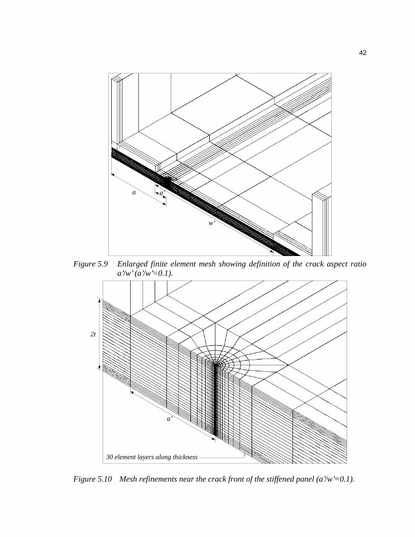
42
Figure 5.9 Enlarged finite element mesh showing definition of the crack aspect ratioa’/w’ (a’/w’=0.1).
Figure 5.10 Mesh refinements near the crack front of the stiffened panel (a’/w’=0.1).
a’
w’
a
2t
a’
30 element layers along thickness

43
6 Results
For the purpose of comparison, the stress intensity factors and T-stresses are
normalized as dimensionless numbers. The normalized stress intensity factor has the form
of ( )aKK πσ ∞= II , while the two normalized T-stresses are defined as ∞= σ1111 TT
and ∞= σ1313 TT , respectively. Here ∞σ is the average stress, computed from the total
nodal force, F due to the far-field displacement ∞u , on the plane of lY = (see Figure 5.1)
divided by the cross-sectional area of the plate. For a cracked plate, ( )wtF=∞σ , where
w is the half width and t is the half thickness. The thickness of the plate is also
normalized because the variations of the stress intensity factor and the T-stresses over the
thickness are to be investigated. The normalized thickness of an element is defined as
txt 3= , which indicates the normalized x3 coordinate at the centroid of the element.
To determine the distribution of the stress intensity factor and the T-stresses over
the thickness of a particular model, these parameters are first calculated from each of the
three adjacent rings of elements very close to the crack front (Rings #2, #3, and #4 as
shown in Figure 5.4) by the equivalent domain integral and interaction integral. Then an
average value is carried out over three domains.
6.1 Isotropic Plates
A family of isotropic plates with different crack lengths and different thicknesses
is examined. The material properties of Young’s modulus Msi10=E and Poisson’s ratio
0.3=ν are used in the modeling. To compare the fracture parameters for different
variables, the stress intensity factor KI and T11 stress are retrieved from the element layer
attached to the centerline of the thickness. As shown in Figure 5.6, this layer has a
thickness of 0.0625t, and the x3 coordinate of the centroid is located at 0.03125t. Hence
IK and 11T of different models will be retrieved and plotted at normalized thickness

44
03125.0=t . The T13 stress is retrieved from the element layer approximately at the
quarter thickness of a plate, or at the thickness between 0.50t and 0.55t, i.e., Layer #9 as
shown in Figure 5.6, and therefore 525.0=t for this element.
6.1.1 Crack Length
First we will consider a plate of thickness in. 0.332 =t ( 00825.0=wt ) with
various crack aspect ratios 0.9~0.1=wa . To compare the effects of the thickness on
fracture parameters for the same crack aspect ratios, the results from another set of plates
with thickness of in. .24102 =t ( 256.0=wt ) are presented as well.
Figure 6.1 shows the distribution of the normalized stress intensity factors IK
over half of the thickness for different crack aspect ratios. The distribution of the stress
intensity factor is symmetric with respect to x3=0. IK is fairly constant over half of the
thickness, except in the region near the free surface (approximately from 8.0≥t for
0.1=wa down to 6.0≥t for 0.9=wa ), where the stress intensity factor slightly
decreases. Note that there exists a weaker corner singularity near the free surface. The
normalized stress intensity factors at the center of thickness are retrieved and plotted
against the a/w ratios in Figure 6.2. The results for in. .1650=t show that IK rises
dramatically from 1.06 at the small crack of 0.1=wa to 2.72 as the a/w ratio reaches
0.9. Results from the other set of plates with thickness of in. 5.12=t ( 256.0=wt ) are
also shown in the same figure, in which the normalized stress intensity factor increases
from 1.00 to 2.64 as the a/w ratios goes from 0.1 to 0.9. It is slightly smaller than that of
the thinner plate.
The 2-D plane strain analytical solution of IK , also shown in Figure 6.2, has the
following form in terms of the crack aspect ratio a/w [38]:
+−
= 42
I )(06.0)(025.01)(2
sec)(w
a
w
a
w
a
w
aK
π. (6.1)

45
When the normalized stress intensity factor obtained from 3-D analysis is compared with
the 2-D solution, i.e. Eq.(6.1), deviation within 4% on the average from the 2-D solution
is found for the thicker plate; more than 5% for the thinner plate.
Figure 6.3 shows the distribution of the normalized T11 stresses over half of the
thickness in the thinner plate ( in. .1650=t ) for different crack aspect ratios. The T11
stress distribution is symmetric with respect to x3=0. For all a/w ratios, the variation of
11T over half of the thickness is relatively small except in the region near the free surface
(approximately 85.0≥t ), where the corner singularity would cause the T11 stress to
diverge. For most curves ( 0.7<wa ), the near-constant part of 11T stays near –1.0,
which is the theoretical 2-D solution. In Figure 6.4 the curve of the thinner plate
( 00825.0=wt ) confirms this trend as the magnitude of the normalized T11 stresses stays
between –0.8 and –1.0 before the crack aspect ratio reaches 0.7. Beyond that the
normalized T11 stress increases (in magnitude) rapidly to –3.77 as the a/w ratio reaches
0.9. The other curve representing the thicker plate shows a similar trend, but the
magnitude of 11T at the center increases from –1.02 at the smallest crack, 0.1=wa , to
87.4− at the largest crack, 0.9=wa .
The 2-D solution of 11T , also shown in Figure 6.4, can be obtained from the stress
biaxiality ratio B and normalized stress intensity factors IK :
I11 KBT = , (6.2)
where B is a function of the crack aspect ratio a/w [39]:
+−= )(085.01)(
w
a
w
aB . (6.3)
Results from the thicker plate are closer to the 2-D solution than those of the thinner
plate, although the closeness is only maintained until a/w is near 0.7. This indicates that,
at a small crack, 11T of the thicker plate is closer to the plane strain condition than that of
the thinner plate.

46
In Figure 6.5, the distribution of the normalized T13 stresses over half of the
thickness of the thinner plate for different a/w ratios does not have a constant portion
shown in the distribution of IK and 11T . Note that the distribution is anti-symmetric with
respect to x3=0. Instead, the magnitude of the normalized T13 stresses rises monotonically
from zero at the center of thickness to a much larger value near the free surface, and
ultimately back to zero to satisfy the stress-free condition at the free surface. The larger
the crack length is, the more sharply the 13T stress results. As the normalized T13 stresses
at 5.0=t are retrieved for all a/w ratios, as shown in Figure 6.6, it is observed for the
thinner plate that the magnitude of the normalized T13 stresses increases from
approximately –0.35 for 0.1=wa to –2.6 for 0.9=wa . For the case of the thicker
plate, the trend persists. The overall variation of 13T , however, is much smaller than that
of the thinner plate. The absolute value of the normalized T13 stresses, which goes from
approximately –0.07 for 0.1=wa up to near –0.6 for 0.9=wa , is relatively smaller.
Note that 013 =T for the 2-D solution.
6.1.2 Plate Thickness
Another set of plates with different thicknesses is analyzed. The crack aspect ratio
of these plates is kept at 0.1=wa . The finite element mesh of each model is also kept
the same; i.e., the overall number of elements is unchanged for each finite element model.
Only the dimensions of the elements are slightly changed due to thickness change. The
thickness ranges from a thinner plate of in. 0.332 =t ( 00825.0=wt ) to a very thick
plate of in. .48202 =t ( 512.0=wt ).
Figure 6.7 shows the variation of normalized stress intensity factors over half of
the thickness for plates with different t/w ratios. It is observed that, for relatively thin
plates ( 064.0≤wt ), IK tends to decrease as t goes away from the center of the plate. In
contrast, for relatively thick plates, IK tends to increase in the thickness beyond the

47
region of 3.0≥t . The variation of IK for all t/w ratios at the center of thickness is
plotted in Figure 6.8. For very thin plates (approximately 03.0≤wt ), the normalized KI
almost stays constant near 1.06. As the thickness increases up to 5.0≥wt , IK gradually
decreases to near 1.0, which is the 2-D solution for very small crack length, i.e.,
0→wa .
The normalized T11 stresses over half of the thickness for plates with different t/w
ratios are plotted in Figure 6.9. The normalized T11 stresses are fairly constant in the
region of 75.0≤t for all cases. Beyond that, 11T in a thinner plate deviates much more
than it would in a relatively thick plate. These stresses, or the normalized T11 stresses at
center of the plate thickness, are extracted and plotted against the t/w ratios in logarithmic
scale in Figure 6.10. The stresses, as shown also in Figure 6.9, increase gradually in
magnitude from approximately –0.79 in a very thin plate ( 004.0=wt ) to –1.01 in a very
thick plate ( 512.0=wt ).
In Figure 6.11, the distribution of the normalized T13 stresses over half of the
thickness rises in magnitude from zero at 0=t to a larger value near the free surface.
This trend is the same as that in Figure 6.5. In general the normalized T13 stresses
decrease in terms of the magnitude as the plate thickness increases. The trend is observed
for the normalized T13 stresses at 5.0=t of each plate in Figure 6.12, in which the
magnitude of 13T decreases from approximately –0.5 for a very thin plate ( 004.0=wt )
to near –0.02 for a very thick plate ( 512.0=wt ).
6.2 Orthotropic Plates
The plates of same dimensions are analyzed again with the properties of a
composite material. The composite is AS4 carbon warp-knit fabric design by Boeing for
the all-composite wing skin in a commercial aircraft [29]. It has the overall orthotropic
material properties that are listed in Table 6.1. The orientation of the material coordinates

48
is referred to the global coordinate system shown in Figure 5.1.
6.2.1 Crack Length
The distribution of the normalized stress intensity factors IK through half of the
thickness for various crack aspect ratios is shown in Figure 6.13. Each curve of the five
different a/w ratios is relatively flat, meaning that IK is almost constant over the
thickness. In fact, the amount of fluctuation of IK is less than 3% and occurs only in the
region where 85.0≥t . In comparison to Figures 6.13 and 6.1, it is observed that IK of
the orthotropic material is more constantly distributed than that of the isotropic material.
The magnitude for each a/w ratio for the orthotropic material is also slightly (about 6%)
smaller. The normalized stress intensity factors at the center of thickness increases from
1.00 to 2.54 as the a/w ratio increases from 0.1 to 0.9, as shown in Figure 6.14. Results
from the thicker plate ( 256.0=wt ) are also shown in the same figure, in which IK
ranges from 1.00 to about 2.52. Figure 6.14 shows that the two curves are almost
identical, indicating that IK is less sensitive to the change of plate thickness in the
orthotropic material.
Figure 6.15 shows the distribution of the normalized T11 stresses through half of
the thickness for various crack lengths in the thin plate ( in. 0.165=t ). Similar to that of
the isotropic material in Figure 6.3, the variation of 11T is not significant except near the
free surface (approximately 85.0≥t ). For the small crack case ( 0.1=wa ), the flat part
of the 11T curve stays around –0.660, which is nearly equal to the material anisotropy
Table 6.1 Material properties of the orthotropic plate.
Msi162.5=XE Msi64.0=YZG 22.0=YZν Msi773.11=YE Mpsi57.0=XZG 29.0=XZν
Msi53.1=ZE Msi479.2=XYG 1758.0=XYν
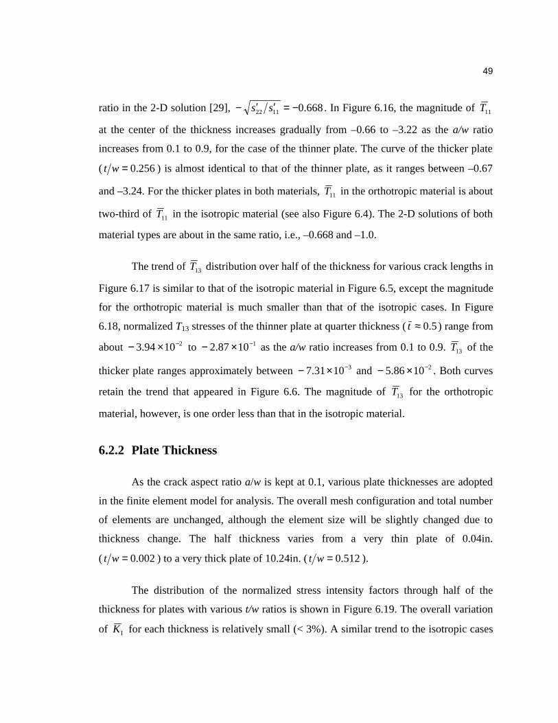
49
ratio in the 2-D solution [29], 668.01122 −=′′− ss . In Figure 6.16, the magnitude of 11T
at the center of the thickness increases gradually from –0.66 to –3.22 as the a/w ratio
increases from 0.1 to 0.9, for the case of the thinner plate. The curve of the thicker plate
( 256.0=wt ) is almost identical to that of the thinner plate, as it ranges between –0.67
and –3.24. For the thicker plates in both materials, 11T in the orthotropic material is about
two-third of 11T in the isotropic material (see also Figure 6.4). The 2-D solutions of both
material types are about in the same ratio, i.e., –0.668 and –1.0.
The trend of 13T distribution over half of the thickness for various crack lengths in
Figure 6.17 is similar to that of the isotropic material in Figure 6.5, except the magnitude
for the orthotropic material is much smaller than that of the isotropic cases. In Figure
6.18, normalized T13 stresses of the thinner plate at quarter thickness (5.0≈t ) range from
about 21094.3 −×− to 11087.2 −×− as the a/w ratio increases from 0.1 to 0.9. 13T of the
thicker plate ranges approximately between 31031.7 −×− and 21086.5 −×− . Both curves
retain the trend that appeared in Figure 6.6. The magnitude of 13T for the orthotropic
material, however, is one order less than that in the isotropic material.
6.2.2 Plate Thickness
As the crack aspect ratio a/w is kept at 0.1, various plate thicknesses are adopted
in the finite element model for analysis. The overall mesh configuration and total number
of elements are unchanged, although the element size will be slightly changed due to
thickness change. The half thickness varies from a very thin plate of 0.04in.
( 002.0=wt ) to a very thick plate of 10.24in. ( 512.0=wt ).
The distribution of the normalized stress intensity factors through half of the
thickness for plates with various t/w ratios is shown in Figure 6.19. The overall variation
of IK for each thickness is relatively small (< 3%). A similar trend to the isotropic cases

50
is that IK tends to decrease in the region of 75.0≥t for thin plates ( 064.0≤wt ) and
increase in the region of 6.0≥t for thick plates. In the region of 5.0≤t , IK of each
case stays very close to 1.0, the 2-D solution for very small crack lengths. IK at the
center of thickness for all t/w ratios is retrieved and plotted in Figure 6.20, in which all
normalized stress intensity factors fall between 0.995 and 1.005. The overall difference is
within 1%. Therefore, IK is rather stable even if the plate thickness increases more than
two orders of magnitude.
Figure 6.21 shows the normalized T11 stresses over half of the thickness for
various t/w ratios. For each plate, 11T is fairly constant in the region of 75.0≤t . In the
region near free surface ( 85.0≥t ), however, 11T tends to diverge as also observed in the
isotropic cases (see Figure 6.9). It is observed that approximately at 8.0=t , all five
curves pass through a point where 11T is near −0.669 that is close to the material
anisotropy ratio, −0.668. 11T at the center of the thickness for all t/w ratios is extracted
and plotted in Figure 6.22. For the plates of 00825.0≥wt , 11T ranges between –0.658
and –0.673, or within %5.1± of the material anisotropy ratio. As the t/w ratio increases
beyond 0.016, i.e., plates with moderate to thick thicknesses, 11T falls within %1± of the
material anisotropy ratio. As the plate becomes thinner ( 006.0≤wt ), however, the
magnitude of 11T decreases from near the material anisotropy ratio to about 90% of that
at 002.0=wt .
In Figure 6.23, a similar trend to the 13T distribution of isotropic plates over half
of the thickness for various t/w ratios is observed. The relative magnitude of 13T for
orthotropic plates is one order less than that in isotropic plates. Figure 6.24 shows 13T at
quarter thickness for all plates. As the plate thickness increases to the very thick case of
512.0=wt , the magnitude of 13T decreases to near zero. All normalized T13 stresses in
orthotropic plates are relatively small, compared to those in isotropic plates.

51
6.3 Stiffened Panels
All stiffened panels have the orthotropic material properties as listed in Table 6.1
and the dimensions as shown in Figure 5.7. Panels with different crack aspect ratios,
a’/w’, ranging from 0.1 to 0.9 are analyzed. To illustrate the effect of crack aspect ratios
on normalized stress intensity factor and the T-stresses, each parameter at the centerline
of the thickness will be plotted against a’/w’ ratios. The value of a parameter is calculated
from the average values over element layers #15 and #16, which are attached on the
centerline. The thickness of each layer is 0.09t. Therefore the centroid is at –0.045t for an
element in Layer #15 and 0.045t for an element in Layer #16.
The original stiffened panel has a thickness of in. 0.332 =t ( 00825.0=wt ). To
compare the effects of panel thickness on the fracture parameters with the same crack
length, the results from another set of thinner panels of 004.0=wt are presented as
well. Note that the stiffener dimensions are fixed for all the normalized studies.
The distribution of the normalized stress intensity factors IK through the entire
thickness of the cracked panels is shown in Figure 6.25. For each crack aspect ratio, the
distribution of IK appears to be increasing almost linearly from the bottom (1−=t ) to
the top ( 1=t ) of the panel thickness. The trend clearly shows the bending effect for
thinner stiffened panels. The slope of each IK curve decreases as the a’/w’ ratio
increases. For instance, IK increases from about 0.8 to 1.9 for 0.1=′′ wa but ranges
only between 0.96 and 1.06 for 0.9=′′ wa . Figure 6.26 shows IK at center of the
thickness for panels with various crack aspect ratios. The normalized stress intensity
factor of the thicker stiffened panel ( 00825.0=wt ) decreases from approximately 1.38
to 1.05, as the a’/w’ ratio increases from 0.1 to 0.9. The thin stiffened panels
( 004.0=wt ) generally have larger IK , which decreases from 1.67 to 1.05 for a’/w’ ratio
from 0.1 to 0.9. The difference of two sets of panels, however, becomes smaller as the

52
crack length increases. Both panels almost have an equal IK of 1.05 at 0.9=′′ wa . It
indicates that, as the crack length becomes large enough, the panel thickness is irrelevant
to the normalized stress intensity factor.
Figure 6.27 shows the distribution of the normalized T11 stresses over the
thickness of the panel for different a’/w’ ratios. The magnitude of 11T is generally in an
increasing trend, although the distribution appears more linearly in larger crack lengths.
Overall, the magnitude of 11T decreases as the crack length increases. This can be
observed in Figure 6.28 where the normalized T11 stresses are extracted and plotted
against different a’/w’ ratios. Though all are negative, 11T of the thicker panel increases
from –0.91 at 0.1=′′ wa to –0.52 at 0.9=′′ wa , while 11T of the thinner panel ranges
from –1.17 to –0.41. For smaller cracks ( 0.7≤′′ wa ), the normalized T11 stress of the
thinner panel is larger (in magnitude) than that of the thicker panel. For larger cracks
( 0.8≥′′ wa ), however, the trend reverses as the thinner panel has a smaller 11T (in
magnitude).
In Figure 6.29, the distribution of 13T through the thickness appears in a nearly
anti-symmetric manner with respect to the thickness centerline, 0=t . The shape of each
13T curve is similar enough that it seems all curves are shifting within a range
approximately equal to 0.5. The overall variation of 13T for all a’/w’ ratios ranges between
–0.1 and –1.5. 13T at center of the thickness for each crack length of both sets of panels is
retrieved and plotted in Figure 6.30. Both curves form part of a parabola, respectively.
For the thicker panels ( 00825.0=wt ), 13T decreases from –0.93 at 0.1=′′ wa to –0.95
at 0.3=′′ wa near the lowest point of the curve, then increases to about –0.58 at
0.9=′′ wa . For the thinner panels, the normalized T13 stress swings from –1.86 at
0.1=′′ wa to –1.22 at 0.9=′′ wa . In between the lowest point is near 0.4=′′ wa
where 13T is approximately –2.16. Figure 6.30 shows the thinner panel has larger 13T (in

53
magnitude) for different crack lengths. And the maximum amplitude of 13T for a panel of
fixed thickness occurs at a moderate crack aspect ratio.

54
KI/(
σ ∞√π
a)
x3/t
0
0.5
1
1.5
2
2.5
3
0 0.25 0.5 0.75 1
a/w=0.1a/w=0.3a/w=0.5a/w=0.7a/w=0.9
Figure 6.1 Normalized stress intensity factors through half of the thickness forisotropic plates of t=0.165 in. (t/w=0.00825) with various a/w ratios.2
Figure 6.2 Normalized stress intensity factors at center of the thickness (x3/t=0) forisotropic plates with two different thicknesses.
KI/(
σ ∞√π
a)
a/w
0.5
1
1.5
2
2.5
3
0 0.2 0.4 0.6 0.8 1
t/w=0.00825t/w=0.2562-D

55
Figure 6.3 Normalized T11 stresses through half of the thickness for isotropic plates oft=0.165 in. (t/w=0.00825) with various a/w ratios.
Figure 6.4 Normalized T11 stresses at center of the thickness (x3/t=0) for isotropicplates with two different thicknesses.
T11
/σ∞
x3/t
-20
-15
-10
-5
0
0 0.25 0.5 0.75 1
a/w=0.1
a/w=0.3
a/w=0.5
a/w=0.7
a/w=0.9
T11
/σ∞
a/w
-5
-4
-3
-2
-1
0
0 0.2 0.4 0.6 0.8 1
t/w=0.00825t/w=0.2562-D

56
Figure 6.5 Normalized T13 stresses through half of the thickness for isotropic plates oft=0.165 in. (t/w=0.00825) with various a/w ratios.
Figure 6.6 Normalized T13 stresses at quarter of the thickness (x3/t=0.5) for isotropicplates with two different thicknesses.
T13
/σ∞
x3/t
-20
-15
-10
-5
0
0 0.25 0.5 0.75 1
a/w=0.1
a/w=0.3
a/w=0.5
a/w=0.7
a/w=0.9
a/w
T13
/σ∞
-3
-2.5
-2
-1.5
-1
-0.5
0
0 0.2 0.4 0.6 0.8 1
t/w=0.00825
t/w=0.256

57
Figure 6.7 Normalized stress intensity factors through half of the thickness forisotropic plates of a/w=0.1 with various t/w ratios.
Figure 6.8 Normalized stress intensity factors at center of the thickness (x3/t=0) forisotropic plates of a/w=0.1.
t/w
KI/(
σ ∞√π
a)
0.8
0.9
1
1.1
1.2
0.001 0.01 0.1 1
KI/(
σ ∞√π
a)
x3/t
0.8
0.9
1
1.1
1.2
0 0.25 0.5 0.75 1
t/w=0.00825
t/w=0.016
t/w=0.064
t/w=0.256
t/w=0.512
a/w=0.1

58
Figure 6.9 Normalized T11 stresses through half of the thickness for isotropic plates ofa/w=0.1 with various t/w ratios.
Figure 6.10 Normalized T11 stresses at center of the thickness (x3/t=0) for isotropicplates of a/w=0.1.
x3/t
T11
/σ∞
-3
-2.5
-2
-1.5
-1
-0.5
0
0 0.25 0.5 0.75 1
t/w=0.00825
t/w=0.016
t/w=0.064
t/w=0.256
t/w=0.512
a/w=0.1
t/w
T11
/σ∞
-1.5
-1.25
-1
-0.75
-0.5
0.001 0.01 0.1 1

59
Figure 6.11 Normalized T13 stresses through half of the thickness for isotropic plates ofa/w=0.1 with various t/w ratios.
Figure 6.12 Normalized T13 stresses at quarter of the thickness (x3/t=0.5) for isotropicplates of a/w=0.1.
x3/t
T13
/σ∞
-2.5
-2
-1.5
-1
-0.5
0
0 0.25 0.5 0.75 1
t/w=0.00825
t/w=0.016
t/w=0.064
t/w=0.256
t/w=0.512
a/w=0.1
t/w
T13
/σ∞
-0.5
-0.4
-0.3
-0.2
-0.1
0
0.001 0.01 0.1 1

60
KI/(
σ ∞√π
a)
x3/t
1
0
0.5
1.5
2
2.5
3
0 0.25 0.5 0.75 1
a/w=0.1a/w=0.3a/w=0.5a/w=0.7a/w=0.9
Figure 6.13 Normalized stress intensity factors through half of the thickness fororthotropic plates of t=0.165 in. (t/w=0.00825) with various a/w ratios.
Figure 6.14 Normalized stress intensity factors at center of the thickness (x3/t=0) fororthotropic plates with two different thicknesses.
KI/(
σ ∞√π
a)
a/w
0.5
1
1.5
2
2.5
3
0 0.2 0.4 0.6 0.8 1
t/w=0.00825
t/w=0.256

61
Figure 6.15 Normalized T11 stresses through half of the thickness for orthotropic platesof t=0.165 in. (t/w=0.00825) with various a/w ratios.
Figure 6.16 Normalized T11 stresses at center of the thickness (x3/t=0) for orthotropicplates with two different thicknesses.
T11
/σ∞
x3/t
-6
-5
-4
-3
-2
-1
0
0 0.25 0.5 0.75 1
a/w=0.1
a/w=0.3
a/w=0.5
a/w=0.7
a/w=0.9
-0.668
T11
/σ∞
a/w
-4
-3.5
-3
-2.5
-2
-1.5
-1
-0.5
0
0 0.2 0.4 0.6 0.8 1
t/w=0.00825
t/w=0.256

62
Figure 6.17 Normalized T13 stresses through half of the thickness for orthotropic platesof t=0.165 in. (t/w=0.00825) with various a/w ratios.
Figure 6.18 Normalized T13 stresses at quarter of the thickness (x3/t=0.5) for orthotropicplates with two different thicknesses.
T13
/σ∞
x3/t
-2
-1.5
-1
-0.5
0
0 0.25 0.5 0.75 1
a/w=0.1
a/w=0.3
a/w=0.5
a/w=0.7
a/w=0.9
a/w
T13
/σ∞
-0.4
-0.3
-0.2
-0.1
0
0 0.2 0.4 0.6 0.8 1
t/w=0.00825
t/w=0.256

63
Figure 6.19 Normalized stress intensity factors through half of the thickness fororthotropic plates of a/w=0.1 with various t/w ratios.
Figure 6.20 Normalized stress intensity factors at center of the thickness (x3/t=0) fororthotropic plates of a/w=0.1.
t/w
KI/(
σ ∞√π
a)
0.9
0.95
1
1.05
1.1
0.001 0.01 0.1 1
KI/(
σ ∞√π
a)
x3/t
0.9
0.95
1
1.05
1.1
0 0.25 0.5 0.75 1
t/w=0.00825
t/w=0.016
t/w=0.064
t/w=0.256
t/w=0.512
a/w=0.1

64
Figure. 6.21 Normalized T11 stresses through half of the thickness for orthotropic platesof a/w=0.1 with various t/w ratios.
Figure 6.22 Normalized T11 stresses at center of the thickness (x3/t=0) for orthotropicplates of a/w=0.1.
-0.668
x3/t
T11
/σ∞
-1
-0.9
-0.8
-0.7
-0.6
-0.5
0 0.25 0.5 0.75 1
t/w=0.00825
t/w=0.016
t/w=0.064
t/w=0.256
t/w=0.512
a/w=0.1
-0.668
t/w
T11
/σ∞
-1
-0.9
-0.8
-0.7
-0.6
-0.5
0.001 0.01 0.1 1

65
Figure 6.23 Normalized T13 stresses through half of the thickness for orthotropic platesof a/w=0.1 with various t/w ratios.
Figure 6.24 Normalized T13 stresses at quarter of the thickness (x3/t=0.5) for orthotropicplates of a/w=0.1.
x3/t
T13
/σ∞
-0.3
-0.25
-0.2
-0.15
-0.1
-0.05
0
0 0.25 0.5 0.75 1
t/w=0.00825
t/w=0.016
t/w=0.064
t/w=0.256
t/w=0.512
a/w=0.1
t/w
T13
/σ∞
-0.1
-0.08
-0.06
-0.04
-0.02
0
0.001 0.01 0.1 1
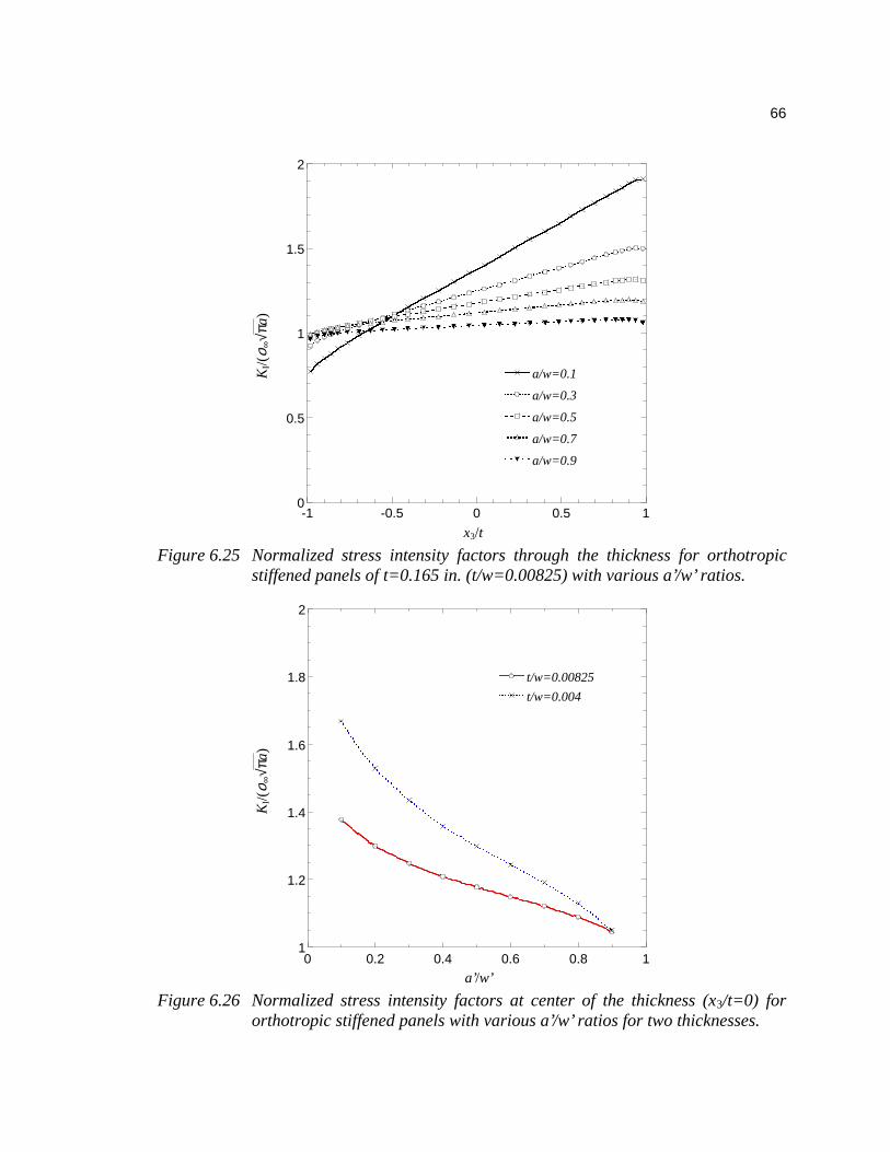
66
KI/(
σ ∞√π
a)
x3/t
0
0.5
1
1.5
2
-1 -0.5 0 0.5 1
a/w=0.1
a/w=0.3
a/w=0.5
a/w=0.7
a/w=0.9
Figure 6.25 Normalized stress intensity factors through the thickness for orthotropicstiffened panels of t=0.165 in. (t/w=0.00825) with various a’/w’ ratios.
Figure 6.26 Normalized stress intensity factors at center of the thickness (x3/t=0) fororthotropic stiffened panels with various a’/w’ ratios for two thicknesses.
KI/(
σ ∞√π
a)
a’/w’
1
1.2
1.4
1.6
1.8
2
0 0.2 0.4 0.6 0.8 1
t/w=0.00825
t/w=0.004

67
Figure 6.27 Normalized T11 stresses through the thickness for orthotropic stiffenedpanels of t=0.165 in. (t/w=0.00825) with various a’/w’ ratios.
Figure 6.28 Normalized T11 stresses at center of the thickness (x3/t=0) for orthotropicstiffened panels with various a’/w’ ratios for two thicknesses.
T11
/σ∞
x3/t
-2
-1.5
-1
-0.5
0
-1 -0.5 0 0.5 1
a/w=0.1
a/w=0.3
a/w=0.5
a/w=0.7
a/w=0.9
T11
/σ∞
a’/w’
-1.2
-1
-0.8
-0.6
-0.4
-0.2
0 0.2 0.4 0.6 0.8 1
t/w=0.00825
t/w=0.004

68
Figure 6.29 Normalized T13 stresses through the thickness for orthotropic stiffenedpanels of t=0.165 in. (t/w=0.00825) with various a’/w’ ratios.
Figure 6.30 Normalized T13 stresses at center of the thickness (x3/t=0) for orthotropicstiffened panels with various a’/w’ ratios for two thicknesses.
T13
/σ∞
x3/t
-2
-1.5
-1
-0.5
0
-1 -0.5 0 0.5 1
a’/w’=0.1
a’/w’=0.3
a’/w’=0.5
a’/w’=0.7
a’/w’=0.9
a’/w’
T13
/σ∞
-2.5
-2
-1.5
-1
-0.5
0 0.2 0.4 0.6 0.8 1
t/w=0.00825
t/w=0.004

69
7 Summary and Conclusions
The equivalent domain integral method is used to determine the point-wise stress
intensity factor, or the distribution of it along a three-dimensional crack front. This
method is modified from J-integral with the use of a weighting function, i.e., the s-
function. In the practice of numerical computation, the finite element shape function is
applied as the s-function.
In addition to the stress intensity factor, a second fracture parameter, namely the
T-stress, is determined in order to better characterize the fracture behavior. The
components of T-stress can be obtained by the evaluation of the interaction integral. The
interaction integral is derived from the equivalent domain integral method with the
concept of an auxiliary field. The auxiliary field is the solution corresponding to uniform
force acting on the crack front. The Stroh formalism is used to derive the auxiliary stress
and displacement fields associated with different T-stress components, such as T11 and
T13, in the monoclinic material with the plane of symmetry at x3=0.
The finite element models are made on two sets of through-thickness center-
cracked plates with isotropic and orthotropic material properties, respectively. Similar
finite element meshes are generated on another set of orthotropic composite panels with
stiffeners. All of these structures are under the mode-I uniform displacement loading.
For plates, the stress intensity factor will increase as the crack length increases in
plates with the same dimension. The effect of material properties on the stress intensity
factors at the center of the plate is not significant and all of the stress intensity factors are
close to the corresponding 2-D solutions, especially for relatively thick plates. For plates
of different thicknesses with the same crack length, the stress intensity factor for isotropic
plates decreases as the thickness increases while for orthotropic plates the trend is
relatively insensitive. For panels with stiffeners, however, the stress intensity factor
decreases as the crack length in the panel increases. Similar to the unstiffened plates, a

70
thinner stiffened panel has a larger stress intensity factor for a given crack length. The
exception occurs for the case of relatively larger crack lengths, e.g., 0.9=′′ wa , where
two sets of thin panels of different thicknesses have nearly identical values of stress
intensity factor.
The T11 stresses in all cases of center-cracked plates and panels are compressive.
Based on the stress field near the crack tip prior to fracture initiation from a couple tests
[29], the crack may not have tendency to turn. This is in contradiction to the experimental
observation that the crack did turn near the stiffener. A possible reason may be due to
other interacting failure modes, such as delamination and disbond with stitched interface,
that caused the turning. Among plates, the magnitude of T11 increases when the crack
length increases, regardless of the material properties or plate thickness. The thickness
effect in plates with a small length of crack is more profound for isotropic ones, in which
the T11 stress increases (in magnitude) as the thickness increases. Although in general the
orthotropic plates have the same trend, the changes of T11 are relatively small for thicker
plates. The trends observed in plates are reversed in stiffened panels, where T11 decreases
(in magnitude) when a crack length in a panel increases. At small crack lengths, T11 in a
thin panel also has a larger magnitude then T11 in a thick panel.
The T13 stress in plates of both materials increases (in magnitude) when the crack
length increases, but a larger magnitude is found in isotropic plates. T13, however,
decreases in magnitude as the plate thickness increases. For very thick plates, where the
plane strain condition dominates near the middle of plate thickness, T13 approaches zero.
This is also true in two-dimensional analysis, in which T11 is the only effective T-stress
component. In stiffened panels, the magnitude of T13 is generally smaller for large cracks.
The largest magnitude of T13, however, is not found in panels with a smallest crack, but
with a somewhat larger crack.
This research may be extended in the future according to the following aspects.
(1) The loading condition may be extended from uniaxial tension to others, such as pure
bending or biaxial loading. The change of the loading conditions, however, may incur
71
mixed-mode effects. If the asymptotic stress field near the crack front includes mixed
modes, the mode-II and mode-III effects must be taken into account for the equivalent
domain integral formulation. The calculation of the stress intensity factors will also
require the consideration of the auxiliary fields [21].
(2) The effects of mixed mode may come from the existence of a kinked crack [40].
However, a fracture plate with the kinked crack requires an even larger finite element
model to simulate because it usually is not considered as a symmetric geometry.
(3) Since the stress intensity factors and the T-stresses are related to the material
properties, a composite material may be designed such that a certain level of the
desired parameters can be obtained.
72
References
[1] A. A. Griffith, The phenomena of rupture and flow in solids. PhilosophicalTransactions of the Royal Society of London, Series A, 221, pp.163-198, 1920.
[2] G. R. Irwin, Onset of fast crack propagation in high strength steel and aluminumalloys. Segamore Research Conference Proceedings, 2, pp.289-305, 1956.
[3] H. M. Westergaard, Bearing pressures and cracks. ASME Journal of AppliedMechanics, 6, pp.49-53, 1939.
[4] G. R. Irwin, Analysis of stresses and strains near the end of a crack traversing aplate. ASME Journal of Applied Mechanics, 24, pp.361-364, 1957.
[5] J. R. Rice, A path independent integral and the approximate analysis of strainconcentration by notches and cracks. ASME Journal of Applied Mechanics, 35,pp.379-386, 1968.
[6] D. M. Parks, The virtual crack extension method for nonlinear material behavior.Computer Methods in Applied Mechanics and Engineering, 12, pp.353-364, 1977.
[7] H. G. deLorenzi, On the energy release rate and the J-integral for 3-D crackconfiguration. International Journal of Fracture, 19, pp.183-193, 1982.
[8] H. G. deLorenzi, Energy release rate calculations by the finite element method.Engineering Fracture Mechanics, 21, No.1, pp.129-143, 1985.
[9] F. Z. Li, C. F. Shih and A. Needleman, A comparison of methods for calculatingenergy release rates. Engineering Fracture Mechanics, 21, No.2, pp.405-421, 1985.
[10] C. F. Shih, B. Moran and T. Nakamura, Energy release rate along a three-dimensional crack front in a thermally stressed body. International Journal ofFracture, 30, pp.79-102, 1986.
[11] T. Nakamura, C. F. Shih and L. B. Freund, Analysis of a dynamically loaded three-point-bend ductile fracture specimen. Engineering Fracture Mechanics, 25, No.3,pp.323-339, 1986.
[12] G. P. Nikishkov and S. N. Atluri, An equivalent domain integral method forcomputing crack-tip integral parameters in non-elastic, thermo-mechanical fracture.Engineering Fracture Mechanics, 26, No.6, pp.851-867, 1987.

73
[13] G. P. Nikishkov and S. N. Atluri, Calculation of fracture mechanics parameters foran arbitrary three-dimensional crack, by the ‘equivalent domain integral’ method.International Journal for Numerical Methods in Engineering, 24, pp.1801-1821,1987.
[14] I. S. Raju and K. N. Shivakumar, An equivalent domain integral method in the two-dimensional analysis of mixed mode crack problems. Engineering FractureMechanics, 37, No.4, pp.707-725, 1990.
[15] K. N. Shivakumar and I. S. Raju, An equivalent domain integral method for three-dimensional mixed-mode fracture problems. Engineering Fracture Mechanics, 42,No.6, pp.935-959, 1992.
[16] K. S. Woo, C. H. Hong and Y. S. Shin, An extended equivalent domain integralmethod for mixed mode fracture problems by the p-version of FEM. InternationalJournal for Numerical Methods in Engineering, 42, pp.857-884, 1998.
[17] T. Nakamura and D. M. Parks, Three-dimensional stress field near the crack front ofa thin elastic plate. ASME Journal of Applied Mechanics, 55, pp.805-813, 1988.
[18] C. F. Shih and R. J. Asaro, Elastic-plastic analysis of cracks on bimaterialinterfaces: part I small scale yielding. ASME Journal of Applied Mechanics, 55,pp.299-315, 1988.
[19] C. F. Shih, B. Moran and T. Nakamura, Crack tip integrals and domain integralrepresentations for three-dimensional crack problems. Analytical, Numerical, andExperimental Aspects of Three-Dimensional Fracture Processes, ASME AMD-Vol. 91, edited by A. J. Rosakis, K. Ravi-Chandar and Y. Rajapakse, pp.125-139,1988.
[20] T. Nakamura, C. F. Shih and L. B. Freund, Three-dimensional transient analysis of adynamically loaded three-point-bend ductile fracture specimen. Nonlinear FractureMechanics: Vol. I Time-Dependent Fracture, ASTM STP 995, edited by A.Saxena, J. D. Landes and J. L. Bassani, pp.217-241, 1989.
[21] T. Nakamura and D. M. Parks, Antisymmetrical 3-D stress field near the crack frontof a thin elastic plate. International Journal of Solids and Structures, 25, No.12,pp.1411-1426, 1989.
[22] M. L. Williams, On the stress distribution at the base of a stationary crack. ASMEJournal of Applied Mechanics, 24, pp.109-114, 1957.
[23] S. G. Larsson and A. J. Carlsson, Influence of non-singular stress terms andspecimen geometry on small-scale yielding at crack tips in elastic-plastic materials.Journal of the Mechanics and Physics of Solids, 21, pp.263-277, 1973.

74
[24] J. R. Rice, Limitations to the small scale yielding approximation for crack tipplasticity. Journal of the Mechanics and Physics of Solids, 22, pp.17-26, 1974.
[25] A. H. Sherry, C. C. France and M. R. Goldthorpe, Compendium of T-stresssolutions for two and three dimensional cracked geometries. Fatigue and Fractureof Engineering Materials and Structures, 18, No.1, pp.141-155, 1995.
[26] B. S. Henry and A. R. Luxmoore, Three-dimensional evaluation of the T-stress incentre cracked plates. International Journal of Fracture, 70, pp.35-50, 1995.
[27] B. Yang and K. Ravi-Chandar, Evaluation of elastic T-stress by the stress differencemethod. Engineering Fracture Mechanics, 64, No.5, pp.589-605, 1999.
[28] T. Nakamura and D. M. Parks, Determination of elastic T-stress along three-dimensional crack fronts using an interaction integral. International Journal ofSolids and Structures, 29, No.13, pp.1597-1611, 1992.
[29] F. G. Yuan and S. Yang, Fracture behavior of stitched warp-knit fabric composites.Accepted by International Journal of Fracture, 2000.
[30] G. P. Nikishkov, Some numerical methods of fracture mechanics based on domaininvariant integrals. Fracture, edited by G. P. Cherepanov, Krieger PublishingCompany, Malabar, FL, U.S.A. pp.542-556, 1998.
[31] K. -J. Bathe, Finite Element Procedures in Engineering Analysis, Prentice-Hall Inc.,Englewood Cliffs, NJ, U.S.A., 1982.
[32] A. P. Kfouri, Some evaluations of the elastic T-term using Eshelby’s method.International Journal of Fracture, 30, pp.301-315, 1986.
[33] F. G. Yuan, Determination of stress coefficient terms in cracked solids formonoclinic materials with plane symmetry at x3=0. NASA Contractor Report,NASA/CR-1998-208729, 1998.
[34] R. M. Jones, Mechanics of Composite Materials, Scripta Book Company,Washington, DC, U.S.A., 1975.
[35] T. C. T. Ting, Anisotropic Elasticity: Theory and Applications, Oxford UniversityPress, Inc., New York, NY, U.S.A., 1996.
[36] S. G. Lekhnitskii, Theory of Elasticity of an Anisotropic Body, Mir Publishers,Moscow, Russia, 1981.
[37] S. Yang and F. G. Yuan, Determination and representation of the stress coefficientterms by path-independent integrals in anisotropic cracked solids. InternationalJournal of Fracture, 101, pp.291-319, 2000.

75
[38] T. L. Anderson, Fracture Mechanics: Fundamentals and Applications, SecondEdition. CRC Press, Boca Raton, Florida, U.S.A., 1995.
[39] P. S. Leevers and J. C. Radon, Inherent stress biaxiality in various fracture specimengeometries. International Journal of Fracture, 19, pp.311-325, 1982.
[40] S. Yang and F. G. Yuan, Kinked crack in anisotropic bodies. International Journalof Solids and Structures, 37, pp. 6635-6682, 2000.

76
Appendices

77
A. ANSYS Program
The following ANSYS program is to generate a finite element model of one-
fourth of a stiffened panel with a center crack. The structural dimensions are described in
Chapter 5, and the material properties are listed in Table 6.1. The program will output
plain text files which includes data of displacements, strains, stresses, nodal coordinates,
and other parameters to be used later in a FORTRAN program. This program is tested on
ANSYS/ResearchFS, the product combination of ANSYS Revision 5.5.1 licensed to the
North Carolina Supercomputing Center. This program can be modified to generate a
finite element model for the simpler center-cracked plate.
ANSYS commands are not case-sensitive, i.e., a command in uppercase is
identical to a command in lowercase. For the purpose of clarity, however, all commands
and associated arguments are listed with uppercase characters, except the user-defined
parameters that use lowercase characters.

78
/BATCH/UNITS,BIN ! British system of units using inches! ================ BEGINNING of Parameters Definition =================! Material Properties*DIM,mat,ARRAY,3,3,1 ! array to store material propertiesmat(1,1) = 5.162e6,11.773e6,1.530e6 ! Ex,Ey,Ezmat(1,2) = 0.22,0.29,5.162/11.773*0.401 ! NUyz,NUxz,NUxymat(1,3) = 0.640e6,0.570e6,2.479e6 ! Gyz,Gxz,Gxy
! Parameters for Loading Conditionsappstn = 0.001 ! applied far-field uniform strain
! Geometric Parameters*DIM,cir,ARRAY,5,1,1 ! array of dimensions of the fan-type areaaow = 0.1 ! a/w ratioplz = 0.33 ! full length of the panel in Z-direction (thickness)plx = 20 ! 1/2 length of the panel in X-direction (w)ply = 40 ! 1/2 length of the panel in Y-direction (l)tst = 0.22 ! 1/2 thickness of the stiffenerhst = 2.3 ! height of the stiffenerwst = 1.6+tst/2 ! 1/2 width of the stiffener (a0)ws1 = wst-tst ! 1/2 width of the base of the stiffenerdxc = 8 ! distance between the center of 2 stiffenersdxe = dxc-2*wst ! distance between the edge of 2 stiffenersdsp = ply*appstn ! applied far-field displacementclp = aow*dxe ! crack length in panel portion (a’)ckl = wst+clp ! 1/2 crack length (a=a0+a’)ctf = dxe-clp ! panel length in front of crack tip
! Parameters for Mesh Control*DIM,neci,ARRAY,3,1,1 ! mesh-control parameters over the fan*DIM,srrl,ARRAY,3,1,1 ! spacing ratios for radial lines*DIM,zkpn,ARRAY,4,1,1 ! keypoint numbers at Z-direction interfaces*DIM,zntk,ARRAY,6,1,1 ! normalized thicknesses for different spacing*DIM,nezi,ARRAY,6,1,1 ! number of elements in each regionneci(1) = 1,12,1srrl(1) = 1,26,1zntk(1) = 0.20,0.35,0.45,0.45,0.35,0.20nezi(1) = 5,5,5,5,5,5narc = 6 ! number of arcs for a 90-degree spanangc = 90/narc ! arc angle per elementnezz = nezi(1)+nezi(2)+nezi(3) ! number of element layers along 1/2! thicknessnerr = neci(2) ! number of elements in r-directionneyf = 6 ! number of solid model divisions in! Y-direction of far-field portionsryf = 32 ! spacing ratio in Y-direction of far-field portion
! Define spacing ratios in X-direction*IF,aow,LE,0.3,THEN nec1 = 2 sr1 = 3 nec2 = 4 sr2 = 10*ELSEIF,aow,GE,0.7,THEN nec1 = 4 sr1 = 10 nec2 = 2 sr2 = 3*ELSE ! 0.3 < a’/w’ < 0.7

79
nec1 = 3 sr1 = 9 nec2 = 3 sr2 = 9*ENDIF
! Define critical length*IF,aow,LE,0.5,THEN ! a’/w’ <= 0.5 *IF,plz,LE,clp,THEN ! (2t<=a’) lcr = plz ! critical length = min[a’,w’-a’,2t] *ELSE ! (2t>a’) lcr = clp ! critical length = min[a’,w’-a’,2t] *ENDIF*ELSE ! a’/w’ > 0.5 *IF,plz,LE,ctf,THEN ! (2t<=w’-a’) lcr = plz ! critical length = min[a’,w’-a’,2t] *ELSE ! (2t>w’-a’) lcr = ctf ! critical length = min[a’,w’-a’,2t] *ENDIF*ENDIF
rac = 0.004*lcr ! radial size of the smallest element (e0)cir(1) = 0,rac,100*rac,150*racdyf = ply-cir(4) ! length in Y-directiontw = (plz/2)/plx ! t/w ratio! ~~~~~~~~~~~~~~~~~~~ END of Parameters Definition ~~~~~~~~~~~~~~~~~~~~
/TITLE,1/4 stiffened panel,a’/w’=%aow%,t/w=%tw%,lcr=%lcr%,e0=%rac%; C. Lin
! ================= BEGINNING of Preprocessing Phase ==================/PREP7ET,1,95,,,,,1 ! element type: SOLID95, the 20-node 3-D structural! element with solution output at integration pointsKEYOPT,1,11,1 ! 2x2x2 reduced integration optionET,2,93 ! SHELL93, 8-node plate elementMP,EX,1,mat(1,1) ! assign material propertiesMP,EY,1,mat(2,1)MP,EZ,1,mat(3,1)MP,PRXY,1,mat(3,2)MP,PRYZ,1,mat(1,2)MP,PRXZ,1,mat(2,2)MP,GXY,1,mat(3,3)MP,GYZ,1,mat(1,3)MP,GXZ,1,mat(2,3)
! Solid Model Generation:! Generate fan-type areas over a span of 90 degreesLOCAL,14,0,ckl,0,-plz/2 ! local Cartisian c.s. #14 at crack tipWPCSYS,1,14 ! set working plane at local c.s. #14*DO,i,1,narc ! generate the innermost ring, Ring #0 PCIRC,cir(1),cir(2),(i-1)*angc,i*angc*ENDDOPCIRC,cir(2),cir(3),0,90 ! annular area to be mapped meshed laterRECTNG,0,cir(4),0,cir(4)ARSYM,X,ALLBTOL,rac/100 ! set Boolean operation toleranceAOVLAP,ALL ! create areas on the x-y planeBTOL,DEFA
! Set line divisions on all circumferencial and radial lines

80
LOCAL,15,1,ckl,0,0 ! local cylindrical c.s. #15 at crack tipLSEL,S,LOC,X,cir(2)LESIZE,ALL,,,1 ! set divisions on circumferencial lines*DO,i,1,3 LSEL,S,LOC,X,(cir(i)+cir(i+1))/2 LESIZE,ALL,,,neci(i),srrl(i) ! set divisions on radial lines*ENDDO
! Concatenate lines around the fan-type area for mapped mesh later*DO,i,1,2 LSEL,S,LOC,X,cir(2) LSEL,R,LOC,Y,(i-1)*90,i*90 LCCAT,ALL LSEL,S,LOC,X,cir(4)/2*SQRT(5) LSEL,R,LOC,Y,(i-1)*90,i*90 LESIZE,ALL,,,narc/2,1 LCCAT,ALL*ENDDOLSEL,ALLNUMCMP,ALL ! compress all numbering
! Mesh areas on X-Y plane/NERR,3 ! turn off warning messagesASEL,S,LOC,X,0,cir(2)AATT,1,1,2MSHAPE,1,2D ! mesh areas containing crack tip with triangle elementsAMESH,ALL ! areas meshed with SHELL93 elementsASEL,INVEAATT,1,1,2MSHAPE,0,2D ! mesh other areas with quadrilateral elementsAMESH,ALL ! areas meshed with SHELL93 elementsLSEL,S,SPACE,,0 ! select concatenated lines to be deletedLDELE,ALL ! delete concatenated lines
! Generate the finite element model along full panel thicknessASEL,ALLTYPE,1 ! designate element type as SOLID95CSYS,0 ! set active c.s. as global Cartesianzi = -plz/2*DO,i,1,6 ! generate SOLID95 elements by extending selected areas ESIZE,,nezi(i) VEXT,ALL,,,,,zntk(i)*plz/2 zi = zi+zntk(i)*plz/2 ! Z-coordinate of the areas to be offset ASEL,S,LOC,Z,zi*ENDDOASEL,S,TYPE,,2,,,1ACLEAR,ALL ! delete all SHELL93 elements
! Construct the other portions of the panelCSYS,14 ! switch to the local Cartesian c.s. on the crack tipNUMSTR,KP,1001NUMSTR,LINE,2001KSEL,S,LOC,Z,0KSEL,R,LOC,Y,0KSEL,R,LOC,X,-cir(4)*GET,nkp1,KP,0,NUM,MAX ! nkp1: keypoint # of this keypointKGEN,2,ALL,,,-(clp-cir(4)) ! keypoint #1001L,nkp1,1001,nec1,sr1 ! line #2001KSEL,S,LOC,Z,0KSEL,R,LOC,Y,0

81
KSEL,R,LOC,X,cir(4)*GET,nkp2,KP,0,NUM,MAX ! nkp2: keypoint # of this keypointKGEN,2,ALL,,,dxe-clp-cir(4) ! keypoint #1002L,nkp2,1002,nec2,sr2 ! line #2002NUMSTR,DEFAASEL,S,LOC,X,-cir(4)VDRAG,ALL,,,,,,2001 ! generate cracked portion of the panelASEL,S,LOC,X,cir(4)VDRAG,ALL,,,,,,2002 ! generate uncracked portion of the panel
! Generate the central stiffenerCSYS,0 ! switch back to global Cartesian c.s.ASEL,S,LOC,X,wstESIZE,,1VEXT,ALL,,,-ws1ASEL,S,LOC,X,tstESIZE,,1VEXT,ALL,,,-tstASEL,S,LOC,Z,plz/2ASEL,R,LOC,X,0,wstESIZE,,1VEXT,ALL,,,,,tstASEL,S,LOC,Z,plz/2+tstASEL,R,LOC,X,0,tstESIZE,,1VEXT,ALL,,,,,hst-tst
! Generate the second stiffenerVSEL,S,LOC,X,tst,wst,,1 ! select volumes on the outer central! stiffenerLOCAL,11,0,dxc/2,0,0 ! set local Cartesian c.s. #11VSYMM,X,ALL ! generate volumes on the inner second stiffenerLOCAL,12,0,dxc,0,0 ! set Cartesian c.s. #12 at the center of the! second stiffenerASEL,S,LOC,X,-tstESIZE,,1VEXT,ALL,,,2*tst ! create volumes in the base of the second stiffenerASEL,S,LOC,Z,plz/2+tstASEL,R,LOC,X,-tst,tstESIZE,,1VEXT,ALL,,,,,hst-tst ! generate volumes in the height of the second! stiffenerVSEL,S,LOC,X,-wst,-tst,,1VGEN,2,ALL,,,wst+tst ! generate volumes in the outer part of the! second stiffener
! Generate the outmost stiffenerVSEL,S,LOC,X,-wst,wst,,1 ! select all volumes in the second stiffenerLOCAL,13,0,1.5*dxc,0,0 ! set Cartesian c.s. #13VSYMM,X,ALL ! generate the entire outmost stiffener
! Generate the uncracked panel and the outmost panelLOCAL,16,0,2*dxc,0,0 ! set Cartesian c.s. #16ASEL,S,LOC,X,-wstASEL,R,LOC,Z,-plz/2,plz/2VEXT,ALL,,,-dxe ! generate the uncracked part of the panelASEL,S,LOC,X,wstASEL,R,LOC,Z,-plz/2,plz/2VEXT,ALL,,,dxe/2 ! generate the outmost part of the panel

82
ALLSEL,ALL,ALLNUMMRG,ALL,1e-6NUMCMP,ALL ! compress all numbering
! Construct the entire FE model by extending areas along Y-axisCSYS,0NUMSTR,KP,1001NUMSTR,LINE,2001KSEL,S,LOC,X,0KSEL,R,LOC,Z,0KSEL,R,LOC,Y,cir(4)*GET,nkp3,KP,0,NUM,MAX ! nkp1: keypoint # of this keypointKGEN,2,ALL,,,,dyf ! keypoint #1001L,nkp3,1001,neyf,sryf ! line #2001ASEL,S,LOC,Y,cir(4)VDRAG,ALL,,,,,,2001 ! the entire finite element model completed
ALLSEL,ALL,ALLNUMMRG,ALL,1e-6NUMCMP,ALL ! compress all numbering/VIEW,1,1,1,1 ! set viewing point for plots/ANGLE,1,-90,XM/AUTO,1/TYPE,ALL,2
ASEL,S,LOC,Y,plyASUM ! calculate the total area on the far-field end*GET,ayt,AREA,0,AREA/OUTPUT,par,dat ! output data in <par.dat> file*STATUS,ayt ! "ayt": total area on the far-field end/OUTPUTASEL,ALLFINISH ! finish generation of the finite element model! ~~~~~~~~~~~~~~~~~~~~~ END of Preprocessing Phase ~~~~~~~~~~~~~~~~~~~~
! ==================== BEGINNING of Solution Phase ====================/SOLUANTYPE,STATIC ! static analysisNSEL,S,LOC,X,0D,ALL,UX,0 ! set X-symmetry boundary conditionsNSEL,R,LOC,Y,0NSEL,R,LOC,Z,-plz/2D,ALL,UZ,0 ! set Z-constraints at the center of plateNSEL,S,LOC,Y,plyD,ALL,UY,dsp ! apply the prescribed displacement at far endNSEL,S,LOC,Y,0NSEL,R,LOC,X,ckl,plxD,ALL,UY,0 ! set Y-symmetry boundary conditionsNSEL,ALLEQSLV,PCG,1e-8 ! use the PCG solverERESX,NO ! ouput integration point results to the nodesSAVESOLVEFINISH! ~~~~~~~~~~~~~~~~~~~~~~~ END of Solution Phase ~~~~~~~~~~~~~~~~~~~~~~~
! ================= BEGINNING of Postprocessing Phase =================/POST1nezt = nezz*2 ! number of element layers along thickness*DIM,cmring,CHAR,3,1,1

83
*DIM,zf,ARRAY,nezt+1,1,1 ! array to store Z-coordinate of every layercmring(1) = ’ring2’,’ring3’,’ring4’srr = srrl(2)**(1/(neci(2)-1)) ! spacing ratio between adjacent! elements in r-directionesr = (cir(3)-cir(2))*(1-srr)/(1-srr**neci(2)) ! element size in r-direction
zf(1) = -plz/2 ! Z-coordinate at bottom of the first layerkring = 3 ! number of rings to be recordedk = 1*DO,i,1,6 ! i: index for mesh-size region (= dimension of "zntk") eszi = zntk(i)*(plz/2)/nezi(i) ! element size (z) in each region *DO,j,1,nezi(i) ! j: index for the number of element layer k = k+1 zf(k) = zf(k-1)+eszi *ENDDO*ENDDO
SET,1NSEL,S,LOC,Y,ply ! select nodes on the far endFSUM ! calculate total nodal force on the far end*GET,fyt,FSUM,0,ITEM,FY/OUTPUT,par,dat,,APPEND*STATUS,fyt ! "fyt": total nodal force on the far end*STATUS,nezt ! number of elements layers along thickness*STATUS,plx*STATUS,plz*STATUS,mat,1,3,1,3*STATUS,appstn*STATUS,ckl*STATUS,narc*STATUS,kring*STATUS,nerr*STATUS,aow/OUTPUTNSEL,ALLCSYS,15 ! activate local cylindrical c.s. at crack tipDSYS,15 ! set display c.s. to #15
! Write stresses, strains, displacements, and nodal coordinates of! every elements into files/OUTPUT,sts,dat ! <sts.dat> file to store stresses/OUTPUT/OUTPUT,stn,dat ! <stn.dat> file to store strains/OUTPUT/OUTPUT,dis,dat ! <dis.dat> file to store displacements/OUTPUT/OUTPUT,node,dat ! <node.dat> file to store node coordinates/OUTPUT
*DO,k,2,kring+1 ! select from Ring #2 to Ring #(kring+1) NSEL,S,LOC,X,rac+esr*(1-srr**(k-1))/(1-srr),rac+esr*(1-srr**k)/(1-srr) CM,cmring(k-1),NODE ! group all nodes in the domain to be integrated *DO,i,1,nezt ! i: index for layer in Z-direction NSEL,R,LOC,Z,zf(i),zf(i+1) CM,nlayer,NODE *DO,j,1,narc*2 ! j: index for element in the same layer NSEL,R,LOC,Y,angc*(j-1),angc*j ESLN,S,1 ! select an element /FORMAT,,E /HEADER,OFF,OFF,OFF,OFF,ON,ON

84
/OUTPUT,sts,dat,,APPEND *MSG,INFO,k,i,j Ring # %I , Segment # %I , Element # %I : PRESOL,S /OUTPUT /OUTPUT,stn,dat,,APPEND *MSG,INFO,k,i,j Ring # %I , Segment # %I , Element # %I : PRESOL,EPEL /OUTPUT /HEADER,OFF,OFF,OFF,OFF,OFF,OFF /OUTPUT,dis,dat,,APPEND *MSG,INFO,k,i,j Ring # %I , Segment # %I , Element # %I : PRNSOL,DOF /OUTPUT /OUTPUT,node,dat,,APPEND *MSG,INFO,k,i,j Ring # %I , Segment # %I , Element # %I : ELIST,ALL,,,0,0 NLIST,ALL,,,,Z,Y,X /OUTPUT CMSEL,S,nlayer *ENDDO CMSEL,S,cmring(k-1) *ENDDO*ENDDO
! Write Strain_33 for every crack-front element./OUTPUT,stn33,dat ! <stn33.dat> file to store strains e_33/OUTPUTNSEL,S,LOC,X,0,racCM,fan,NODE ! group all nodes in the fan-type domain/FORMAT,,E/HEADER,OFF,OFF,OFF,OFF,ON,ON
*DO,i,1,nezt ! i: index for layer in Z-direction NSEL,R,LOC,Z,zf(i),zf(i+1) CM,nlayer,NODE NSEL,R,LOC,X,0 ! select 3 nodes on the crack front CM,nfront,NODE CMSEL,S,nlayer *DO,j,1,narc*2 ! j: index for element in the same layer NSEL,R,LOC,Y,angc*(j-1),angc*j *IF,j,GT,1,THEN CMSEL,A,nfront *ENDIF ESLN,S,1 ! select an element /OUTPUT,stn33,dat,,APPEND *MSG,INFO,0,i,j Ring # %I , Segment # %I , Element # %I : PRESOL,EPEL /OUTPUT CMSEL,S,nlayer *ENDDO CMSEL,S,fan*ENDDO
/HEADER,DEFANSEL,ALL

85
ESEL,ALLDSYS,0CSYS,0FINISH! ~~~~~~~~~~~~~~~~~~~~ END of Postprocessing Phase ~~~~~~~~~~~~~~~~~~~~
/EXIT

86
B. FORTRAN Program
The following FORTRAN program is used to calculate the stress intensity factor
and the T-stresses along a three-dimensional crack front in the stiffened panel. The crack
is under mode-I loading (either a uniform displacement or a uniform stress) on the far
ends of the structure. The material type can be isotropic or orthotropic. The general input
of the program is from data files containing stresses, strains, displacements, nodal
coordinates and other associated parameters that are generated from a finite element
analysis run by ANSYS.
The program is created and tested in the Microsoft Fortran PowerStation 4.0, a
commercially available FORTRAN development software for Windows NT and
Windows 95 operating systems. Although the Fortran PowerStation 4.0 incorporates all
the features of Fortran 90, this program is intentionally written by the FORTRAN 77
syntax. This arrangement would maintain the flexibility that the program can be also run
on the platforms that still carry FORTRAN 77. However, the program employs some of
the IMSL libraries, the integrated mathematical and statistical functions, which may not
be available on every platform with the FORTRAN capability.

87
PROGRAM T_STRESSC This program calculates the stress intensity factor K_I and the T-stressC components of T11, T13 and T33 of a 3-D crack problem.C The capabilities of the program in calculation of the finite elementC model are 50 element layers along the crack front, 24 elements per 180C degrees.
C Definition of Selected Variables:C ADISP(i,j) Array for the auxiliary displacement field (for T11) within anC element. i=1..20. j=1..3.C ADISP13(i,j) Array for the auxiliary displacement field (for T13) withinC an element. i=1..20. j=1..3.C APPSTN Far-field strain.C APPSTS Applied far-field stress.C ARC Arc length (in degree) of a single elementC ASTRN(i,j) Array for the auxiliary strain field (for T11) within anC element. i=1..8. j=1..6.C ASTRN13(i,j) Array for the auxiliary strain field (for T13) within anC element. i=1..8. j=1..6.C ASTRS(i,j) Array for the auxiliary stress field (for T11) within anC element. i=1..8. j=1..6.C ASTRS13(i,j) Array for the auxiliary stress field (for T13) within anC element. i=1..8. j=1..6.C AYT Total cross sectional area on the far end.C COORD(i,j) Array for the j-th local cylindrical coordinates of the i-thC node of the element. i=1..20.C COORDL(i,j) Array for the j-th local Cartesian coordinates of the i-thC node of the element. i=1..20.C CPL(i,j) Array for the 6x6 compliance matrix.C CPLR(i,j) Array for the 5x5 reduced compliance matrix.C CRKL 1/2 crack length.C DISP(i,j) Aarray for the displacements of the i-th node, i=1..20. j=1..3C representing UX, UY, and UZ, respectively.C EM(i) Array for 3 Young’s moduli.C ES Element thickness, or the length of "delta".C EZZ(i) Array for the average Ezz strains within an element.C EZZA(i) Array for the average Ezz strains of an element layer.C EX Young’s modulus of the isotropic material.C F Area under the s-function curve.C FF Magnitude of the uniform force on the crack front.C FYT Total nodal force on the far end.C GM(i) Array for 3 shear moduli.C IRING Number of the element rings to be computed.C K2(i) Array for the square of the Stroh normalization factors.C LOAD Loading ID number. 1=fixed displacement, 2=fixed stress.C MAT Material ID number. 1=anisotropic, 2=isotropic.C MIE(i,j) Array for the global element number at the j-th location of theC i-th layer(segment).C MNE(i,j,k) Array for the global node number at the j-th location of theC i-th layer(segment). k=1..20 is the local node number.C MU(i,j) Array for the Storh eigenvalues.C N180 Number of the elements per 180 degrees.C N90 Number of the elements per 90 degrees.C NSEG Number of the element layers(segments) along crack front.C PL Location for the integration points.C PLX 1/2 panel width.C PLZ Panel thickness.C PR Poisson’s ratio of the isotropic material.C PRM(i) Array for 3 Poisson’s ratios.C RG(i),SG(i),TG(i) Arrays for the natural coordinates of Gaussian

88
C integration points, i=1..8.C S11P The 1-1 component of the reduced compliance, s11’.C SIF1(i,j) Array for the value of the stress intesity factor in the i-thC element layer of the j-th ring.C SIF1N(i,j) Array for the value of the normalized stress intesity factor inC the i-th element layer of the j-th ring.C SIF1NAVG(i,2) The average normalized stress intensity factor.C SINF Equivalent far-field stress.C STRN(i,j) Array for the FE result of strains within an element. TheC i-th row stores strain components at the i-th GaussianC integration point, i=1..8. Strain components from 1st to 6thC column are [Exx,Eyy,Ezz,Exy,Eyz,Exz], respectively.C STRS(i,j) Array for FE result of stresses within an element. See "STRN"C for similar definition.C T11(i,j) Array for the value of the T11 stress in the i-th element layerC of the j-th ring.C T11N(i,j) Array for the value of the normalized T11 stress in the i-thC element layer of the j-th ring.C T13(i,j) Array for the value of the T13 stress in the i-th element layerC of the j-th ring.C T13N(i,j) Array for the value of the normalized T13 stress in the i-thC element layer of the j-th ring.C T33(i,j) Array for the value of the T33 stress in the i-th element layerC of the j-th ring.C T33N(i,j) Array for the value of the normalized T33 stress in the i-thC element layer of the j-th ring.C T11NAVG(i,2) The average normalized T11 stress in the i-th layer.C T13NAVG(i,2) The average normalized T13 stress in the i-th layer.C T33NAVG(i,2) The average normalized T33 stress in the i-th layer.C THICK(i,j) Array for Z-coordinate (j=1 global; j=2 normalized) of theC center of the i-th segment, i.e. the "s" corresponding to theC local I(s).C UMINU Difference of mu1 and mu2 (Stroh eigenvalues).C UPLUS Sum of mu1 and mu2 (Stroh eigenvalues).C UPROD Product of mu1 and mu2 (Stroh eigenvalues).C VEDI(i,j) Aarray for the value of local I(s) (equivalent domainC integral of the i-th segment) in the j-th ring.C VII(i,j) Aarray for the value of local I(s) (interaction integralC of the i-th segment) for T11 in the j-th ring.C VI2(i,j) Aarray for the value of local I(s) (interaction integralC of the i-th segment) for T13 in the j-th ring.C X0J(i,j,k) Array for the value of the equivalent domain integral ofC each element. i=1..IRING; j=1..NSEG.C X1J(i,j,k) Array for the value of the interaction integral of eachC element for T11. i=1..IRING; j=1..NSEG.C X2J(i,j,k) Array for the value of the interaction integral of eachC element for T13. i=1..IRING; j=1..NSEG.
IMPLICIT DOUBLE PRECISION (A-H,O-Z) COMPLEX(8) MU(3,2),K2,P,Q,UPLUS,UMINU,UPROD PARAMETER (FF = 1) CHARACTER HEAD*40,RING*7 DIMENSION RING(6) DATA RING /’RING #2’,’RING #3’,’RING #4’,’RING #5’,’RING #6’,’RING + #7’/ COMMON PI,PL,HEAD COMMON /AUX/ ASTRS(8,6),ASTRN(8,6),ADISP(20,3) COMMON /AUX13/ ASTRS13(8,6),ASTRN13(8,6),ADISP13(20,3) COMMON /FESOL/ DISP(21,3),STRS(8,6),STRN(8,6) COMMON /FEMOD/ MIE(50,24),MNE(50,24,20),COORD(21,3),COORDL(20,3)

89
COMMON /MATL/ CPL(6,6),CPLR(5,5),EX,PR COMMON /MUS/ UPLUS,UMINU,UPROD,B,D,K2(3),P(2,2),Q(2,2) COMMON /GIP/ RG(8),SG(8),TG(8) DIMENSION EM(3),GM(3),PRM(3),CPLN(3) DIMENSION VEDI(50,6),VII(50,6),X0J(4,50,24),X1J(4,50,24) DIMENSION EZZ(24),EZZA(50),THICK(50,3),SIF1(50,6),T11(50,6) DIMENSION SIF1N(50,6),T11N(50,6) DIMENSION VI2(50,6),X2J(4,50,24),T13(50,6),T13N(50,6) DIMENSION T33(50,6),T33N(50,6) DIMENSION SIF1NAVG(50,2),T11NAVG(50,2),T13NAVG(50,2),T33NAVG(50,2) OPEN (1,FILE=’sts.dat’,STATUS=’unknown’) ! stress data file OPEN (2,FILE=’stn.dat’,STATUS=’unknown’) ! strain data file OPEN (3,FILE=’dis.dat’,STATUS=’unknown’) ! displacement data file OPEN (4,FILE=’node.dat’,STATUS=’unknown’) ! nodal data file OPEN (5,FILE=’tsts.out’,STATUS=’unknown’) ! parameter output file OPEN (8,FILE=’stn33.dat’,STATUS=’unknown’) ! crack-front strain data file OPEN (9,FILE=’par.dat’,STATUS=’unknown’) ! parameter data file OPEN (12,FILE=’K1N.out’,STATUS=’unknown’) OPEN (13,FILE=’T11N.out’,STATUS=’unknown’) OPEN (24,FILE=’T13N.out’,STATUS=’unknown’) OPEN (25,FILE=’T33N.out’,STATUS=’unknown’)
PI = ACOS(-1.0) PL = 1.0/SQRT(3.0) ! location for integration points
C...Read parameters: READ (9,’(I1,TR4,I1)’) MAT,LOAD READ (9,’(/////TR11,E16.9)’) AYT IF (MAT .EQ. 1) WRITE (5,’("Material: Anisotropic")’) IF (MAT .EQ. 2) WRITE (5,’("Material: Isotropic")’) IF (LOAD .EQ. 1) WRITE (5,’("Far-field loading: Fixed Displacement +")’) IF (LOAD .EQ. 2) WRITE (5,’("Far-field loading: Fixed Load")’) READ (9,’(/////TR11,E16.9)’) FYT IF (LOAD .EQ. 1) WRITE (5,’(A23,1P,E16.9)’) ’Total Nodal Force FY += ’,FYT WRITE (5,’(A22,E14.7)’) ’Cross-sectional area =’,AYT READ (9,’(/////TR12,I2)’) NSEG WRITE (5,’(A17,I3)’) ’No. of Segments =’,NSEG READ (9,’(/////TR11,F11.9)’) PLX WRITE (5,’(A18,1P,E13.6,A3)’) ’1/2 Panel width = ’,PLX,’in’ READ (9,’(/////TR11,E16.9)’) PLZ WRITE (5,’(A23,E13.6,A3)’) ’Full Panel Thickness = ’,PLZ,’in’ GOTO (1,6) MAT ! read mat’l properties based on the mat’l type1 READ (9,3) (EM(K),K=1,3),(PRM(K),K=1,3),(GM(K),K=1,3)3 FORMAT (/////9(TR28,E16.9/))4 FORMAT (3(E14.10,5X)/,3(F11.10,8X)/,3(E14.10,5X)) WRITE (5,5) (EM(K),K=1,3),(PRM(K),K=1,3),(GM(K),K=1,3)5 FORMAT (’Ex,Ey,Ez = ’,3(1P,E16.9,1X),’ psi’,/’NUyz,NUxz,NUxy = ’, +3(0P,F11.9,1X),/’Gyz,Gxz,Gxy = ’,3(1P,E16.9,1X),’ psi’) GOTO (7,8) LOAD ! determine load type6 READ (9,’(/////TR11,E15.8)’) EX WRITE (5,’(A21,E15.8,A4)’) "Young’s Modulus Ex = ",EX,"psi" READ (9,’(/////TR12,E15.9)’) PR WRITE (5,’(A22,F6.4)’) "Poisson’s Ratio nuxy = ",PR GOTO (7,8) LOAD ! determine load type7 READ (9,’(/////TR11,E16.9/)’) APPSTN WRITE (5,’(A18,1P,E13.6)’) ’Far-field strain = ’,APPSTN SINF = ABS(FYT/AYT) ! equivalent far-field stress GOTO 9

90
8 READ (9,’(/////TR12,E15.8/)’) APPSTS WRITE (5,’(A17,1P,E13.6,A4)’) ’Far-field load = ’,APPSTS,’psi’ SINF = APPSTS9 WRITE (5,’(A30,1P,E13.6,A4)’) ’Equivalent far-field stress = ’, +SINF,’psi’ READ (9,’(////TR12,E13.6)’) CRKL WRITE (5,’(A18,1P,E13.6,A3)’) ’1/2 crack length = ’,CRKL,’in’ READ (9,’(/////TR12,I1)’) N90 N180 = N90*2 ARC = 180/N180 ! arc length (in degree) of a single element WRITE (5,’(A30,I2)’) ’Elements in 180-degree span = ’,N180 WRITE (5,’(A28,F5.1,A8)’) ’Arc length of each element =’,ARC, +’Degrees’ READ (9,’(/////TR12,I1)’) IRING WRITE (5,’(A33,I1)’) ’Number of rings to be computed = ’,IRING GOTO (11,36) MAT
C...Evaluate the full and reduced compliance matrices for the anisotropicC material:11 CALL STRUC(EM,GM,PRM) WRITE (5,12) ’Structural Compliance Matrix [S] = ’, +((CPL(I,J),J=1,6),I=1,6)12 FORMAT (/A50/,6(6(1P,E13.6,1X)/)) WRITE (5,13) ’Reduced Structural Compliance Matrix "S_0" = ’, +((CPLR(I,J),J=1,5),I=1,5)13 FORMAT (/A46/,5(5(1P,E13.6,1X)/)) WRITE (5,’(A18,1P,E12.5)’) "Sqrt(s22’/s11’) = ", +SQRT(CPLR(2,2)/CPLR(1,1))C...Solve for Storh eigenvalues: CALL STROH(MU) WRITE (5,21) ’Stroh Eigenvalues =’,((MU(M,N),N=1,2),M=1,3)21 FORMAT (/A20/,3(2(’(’,1P,E13.6,’ + ’,1P,E13.6,’i )’,5X)/)) WRITE (5,22) ’p: ’,(M,(P(M,N),N=1,2),M=1,2) WRITE (5,22) ’q: ’,(M,(Q(M,N),N=1,2),M=1,2)22 FORMAT (A3/,2(I1,2X,2(’(’,1P,E13.6,’ + ’,1P,E13.6,’i )’,5X)/)) WRITE (5,23) ’k^2: ’,(M,K2(M),M=1,3)23 FORMAT (A5/,3(I1,2X,’(’,1P,E13.6,’ + ’,1P,E13.6,’i )’/))C...Calculate L_22 value, for later calculation of K_I: UPLUS = MU(1,1)+MU(2,1) ! sum of 2 eigenvalues UPROD = MU(1,1)*MU(2,1) ! product of 2 eigenvalues A1 = DREAL(UPLUS) ! real part of UPLUS A2 = DREAL(UPROD) ! real part of UPROD B = DIMAG(UPLUS) ! imaginary part of UPLUS D = DIMAG(UPROD) ! imaginary part of UPROD AB = A1*D-A2*B BL22I = CPLR(1,1)*AB ! L_inverse_22 CPLN(1) = CPL(1,1) ! compliance s11 CPLN(2) = CPL(1,3) ! compliance s13 CPLN(3) = CPL(3,3) ! compliance s33 BL21 = -D/(CPLR(1,1)*(B*AB-D**2)) ! L21 BL22 = B/(CPLR(1,1)*(B*AB-D**2)) ! L22 CPLN(1) = CPL(1,1) ! compliance s11 CPLN(2) = CPL(1,3) ! compliance s13 CPLN(3) = CPL(3,3) ! compliance s33 GOTO 40
C...For isotropic materials:36 CPLN(1) = 1/EX CPLN(2) = -PR/EX CPLN(3) = 1/EX

91
BL22 = EX/(2*(1-PR**2))
C...Set Gauss integration point locations within an element:40 CALL GUASS S11P = CPLN(1)-CPLN(2)**2/CPLN(3) ! s11’
C...Calculate the equivalent domain integral and the interaction integral inC every element: DO 300 KR = 1,IRING ! KR: counter for the rings DO 200 I = 1,NSEG ! I: counter for the element layers(segments)C...Array initialization: IF (KR .EQ. 1) THEN ! initialization for later average calculation SIF1NAVG(I,1) = 0 T11NAVG(I,1) = 0 T13NAVG(I,1) = 0 T33NAVG(I,1) = 0 ENDIF VEDI(I,KR) = 0 VII(I,KR) = 0 VI2(I,KR) = 0 IF (KR .EQ. 1) THEN EZZA(I) = 0 ENDIF DO 100 J = 1,N180 ! J: counter for the elements in a segment CALL FERST(I,J)
C...Set up auxiliary fields:61 CALL AUXT13(MU,ARC,MAT) ! auxiliary field for T13 GOTO (62,63) MAT62 CALL AUXAN(MU,ARC) ! auxiliary field for T11 - anisotropic GOTO 7063 CALL AUXI(ARC) ! auxiliary field for T11 - isotropic
C...Evaluate equivalent domain integral and interaction integral:70 CALL INTEG(KR,I,J,X0J,X1J,X2J) VEDI(I,KR) = VEDI(I,KR)+X0J(KR,I,J) ! equivalent domain integral VII(I,KR) = VII(I,KR)+X1J(KR,I,J) ! interaction integral for T11 VI2(I,KR) = VI2(I,KR)+X2J(KR,I,J) ! interaction integral for T13
C...Calculate average Ezz strain in every element on the crack front: IF (KR .EQ. 1) THEN CALL STRN33(EZZ,J) EZZA(I) = EZZA(I)+EZZ(J) ENDIF100 CONTINUE IF (KR .EQ. 1) THEN EZZA(I) = EZZA(I)/N180 ! average over a layer(segment) ENDIF
C...Calculate T-stress and K1 using interaction-integral approach. ES = COORDL(5,3)-COORDL(1,3) ! element thickness F = (2./3.)*ES THICK(I,1) = (COORDL(1,3)+COORDL(5,3))/2 ! local "s" coordinate THICK(I,2) = THICK(I,1)/(PLZ/2) ! normalized thickness THICK(I,3) = COORDL(1,3)/(PLZ/2) ! local "s" coordinate at* bottom of the element VEDI(I,KR) = 2*VEDI(I,KR)/F VII(I,KR) = 2*VII(I,KR)/F VI2(I,KR) = 2*VI2(I,KR)/F GOTO (111,112) MAT

92
C...For anisotropic materials:111 SIF1(I,KR) = SQRT(2*VEDI(I,KR)/BL22I) T11(I,KR) = 1*(VII(I,KR)-EZZA(I)*CPL(1,3)/CPL(3,3))/CPLR(1,1) T13(I,KR) = VI2(I,KR)/CPLR(5,5) T33(I,KR) = (EZZA(I)-(CPL(1,3)*T11(I,KR)+CPL(3,5)*T13(I,KR)))/ + CPL(3,3) GOTO 113C...For isotropic materials:112 SIF1(I,KR) = SQRT(VEDI(I,KR)*EX/(1-PR**2)) T11(I,KR) = 1*(EX/((1-PR**2)*FF))*(VII(I,KR)+FF*PR*EZZA(I)) T13(I,KR) = (EX/(2*(1+PR)))*VI2(I,KR) T33(I,KR) = EX*EZZA(I)+PR*T11(I,KR)
113 SIF1N(I,KR) = SIF1(I,KR)/(SINF*SQRT(PI*CRKL)) T11N(I,KR) = T11(I,KR)/SINF T13N(I,KR) = T13(I,KR)/SINF T33N(I,KR) = T33(I,KR)/SINF SIF1NAVG(I,1) = SIF1NAVG(I,1)+SIF1N(I,KR) T11NAVG(I,1) = T11NAVG(I,1)+T11N(I,KR) T13NAVG(I,1) = T13NAVG(I,1)+T13N(I,KR) T33NAVG(I,1) = T33NAVG(I,1)+T33N(I,KR) IF (KR .EQ. IRING) THEN ! average over rings SIF1NAVG(I,2) = SIF1NAVG(I,1)/IRING T11NAVG(I,2) = T11NAVG(I,1)/IRING T13NAVG(I,2) = T13NAVG(I,1)/IRING T33NAVG(I,2) = T33NAVG(I,1)/IRING ENDIF200 CONTINUE300 CONTINUE
C...Output calculated T-stresses and K1 data: WRITE (12,301) ’SEGMENT’,’THICKNESS’,(RING(K),K=1,IRING),’AVERAGE’ WRITE (13,301) ’SEGMENT’,’THICKNESS’,(RING(K),K=1,IRING),’AVERAGE’ WRITE (24,301) ’SEGMENT’,’THICKNESS’,(RING(K),K=1,IRING),’AVERAGE’ WRITE (25,301) ’SEGMENT’,’THICKNESS’,(RING(K),K=1,IRING),’AVERAGE’301 FORMAT (A7,1X,A9,4X,4(4X,A7,4X))302 FORMAT (I4,4X,F9.6,6(2X,1P,E13.6)) DO 310 I = 1,NSEG WRITE (12,302) I,THICK(I,2),(SIF1N(I,K),K=1,IRING),SIF1NAVG(I,2) WRITE (13,302) I,THICK(I,2),(T11N(I,K),K=1,IRING),T11NAVG(I,2) WRITE (24,302) I,THICK(I,2),(T13N(I,K),K=1,IRING),T13NAVG(I,2) WRITE (25,302) I,THICK(I,2),(T33N(I,K),K=1,IRING),T33NAVG(I,2)310 CONTINUE
999 STOP END
SUBROUTINE STRUC(YOUNG,SHEAR,PSNR)* * * * * * * * * * * * * * * * * * * * * * * * * * * * * * * * * * * * * * * ** The subroutine computes the full and reduced compliance matrices. ** ** --- Subroutine input: YOUNG,SHEAR,PSNR ** --- Subroutine output: CPL,CPLR ** ** --- Definition of local variables: ** C(i,j) Array for the stiffness matrix. ** C0(i,j) Array for the reduced stiffness matrix. ** PSNR(i) Array for 3 Poisson’s ratios. ** SHEAR(i) Array for 3 shear moduli. *

93
* YOUNG(i) Array for 3 Young’s moduli. ** * * * * * * * * * * * * * * * * * * * * * * * * * * * * * * * * * * * * * * * IMPLICIT DOUBLE PRECISION (A-H,O-Z) COMMON /MATL/ CPL(6,6),CPLR(5,5),EX,PR DIMENSION YOUNG(3),SHEAR(3),PSNR(3) DIMENSION C(6,6),C0(5,5)
C...Construct the 6x6 compliance matrix [S]: DO 915 I = 1,3 CPL(I,I) = 1/YOUNG(I) CPL(I+3,I+3) = 1/SHEAR(I)915 CONTINUE CPL(2,1) = -(PSNR(3)/YOUNG(1)) CPL(1,2) = CPL(2,1) CPL(3,1) = -(PSNR(2)/YOUNG(1)) CPL(1,3) = CPL(3,1) CPL(3,2) = -(PSNR(1)/YOUNG(2)) CPL(2,3) = CPL(3,2)
C...Evaluate the 6x6 stiffness matrix [C], the 5x5 reduced stiffness and theC compliance matrices: CALL DLINRG(6,CPL,6,C,6) ! IMSL Library for matrix inversion DO 920 I = 1,5 DO 920 J = 1,5 IF ((I .NE. 3) .AND. (J .NE. 3)) THEN C0(I,J) = C(I,J) ELSEIF ((J .EQ. 3) .AND. (I .NE. 3)) THEN C0(I,J) = C(I,6) ELSEIF ((I .EQ. 3) .AND. (J .NE. 3)) THEN C0(I,J) = C(6,J) ENDIF920 CONTINUE C0(3,3) = C(6,6) CALL DLINRG(5,C0,5,CPLR,5) ! IMSL Library for matrix inversion RETURN END
SUBROUTINE STROH(U)* * * * * * * * * * * * * * * * * * * * * * * * * * * * * * * * * * * * * * * ** The subroutine determines the Stroh eigenvalues from the reduced ** structural compliance matrix. ** ** --- Subroutine input: CPLR ** --- Subroutine output: U,K2,P,Q ** ** --- Definition of local variables: ** A1(i) Array for the 5 coefficients in solving the in-plane ** characteristic equation. ** U(m,n) Array for the Stroh eigenvalues. m=1..3, 3 pairs of eigenvalues** and m=3 indicates the out-of-plane eigenvalue. n=2 is the ** conjugate of n=1. ** Z(i) Array for the 4 roots of the in-plane characteristic equation. ** * * * * * * * * * * * * * * * * * * * * * * * * * * * * * * * * * * * * * * * IMPLICIT DOUBLE PRECISION (A-H,O-Z) COMPLEX(8) U,Z,D2,K2,P,Q,UPLUS,UMINU,UPROD COMMON /MATL/ CPL(6,6),CPLR(5,5),EX,PR COMMON /MUS/ UPLUS,UMINU,UPROD,B,D,K2(3),P(2,2),Q(2,2) DIMENSION U(3,2),A1(5),Z(4)
C...Solve for 4 in-plane eigenvalues:
94
A1(1) = CPLR(2,2) ! coefficient for mu^0: "s’_22" A1(2) = -2*CPLR(2,3) ! coefficient for mu^1: "-2*s’_26" A1(3) = 2*CPLR(1,2)+CPLR(3,3) ! coefficient for mu^2 A1(4) = -2*CPLR(1,3) ! coefficient for mu^3: "-2*s’_16" A1(5) = CPLR(1,1) ! coefficient for mu^4: "s’_11"C...Use an IMSL Library to find the roots of a polynomial with realC coefficients by Laguerre’s method: CALL DZPLRC(4,A1,Z) U(1,1) = Z(1) ! "mu1" U(1,2) = Z(2) ! "mu1_bar" U(2,1) = Z(3) ! "mu2" U(2,2) = Z(4) ! "mu2_bar" UMINU = U(1,1)-U(2,1) ! "mu1-mu2"C...Solve for 2 out-of-plane eigenvalues: A2 = CPLR(5,5) ! coefficient for mu^2: "s’_55" B2 = -2*CPLR(4,5) ! coefficient for mu^1: "-2*s’_45" C2 = CPLR(4,4) ! coefficient for mu^0: "s’_44" D2 = B2**2-4*A2*C2 U(3,1) = (-B2+SQRT(D2))/(2*A2) ! "mu3" U(3,2) = (-B2-SQRT(D2))/(2*A2) ! "mu3_bar"C...Calculate p, q, and normalization factors k: DO 935 N = 1,2 P(N,1) = CPLR(1,1)*U(N,1)**2-CPLR(1,3)*U(N,1)+CPLR(1,2) ! "p1" P(N,2) = CONJG(P(N,1)) ! "p1_bar" Q(N,1) = CPLR(1,2)*U(N,1)-CPLR(2,3)+CPLR(2,2)/U(N,1) ! "q1" Q(N,2) = CONJG(Q(N,1)) ! "q1_bar" K2(N) = 1/(2*(Q(N,1)-U(N,1)*P(N,1))) ! k1^2, k2^2935 CONTINUE K2(3) = 1/(2*(CPLR(4,4)/U(3,1)-CPLR(4,5))) ! k3^2990 RETURN END
SUBROUTINE GUASS* * * * * * * * * * * * * * * * * * * * * * * * * * * * * * * * * * * * * * * ** The subroutine defines the Gaussian integration point locations using ** reduced 8-point rule. ** ** --- Subroutine input: none ** --- Subroutine output: RG,SG,TG ** ** --- Definition of local variables: ** PL1 Integration point location. ** RI,SI,TI Coeffecients for the integration point locations. ** * * * * * * * * * * * * * * * * * * * * * * * * * * * * * * * * * * * * * * * IMPLICIT DOUBLE PRECISION (A-H,O-Z) COMMON /GIP/ RG(8),SG(8),TG(8) DIMENSION SI(8),TI(8),RI(8) DATA RI /-1,1,1,-1,-1,1,1,-1/ DATA SI /-1,-1,1,1,-1,-1,1,1/ DATA TI /-1,-1,-1,-1,1,1,1,1/
PL1 = 1/SQRT(3.0) ! point location for integrationC...Set up 2x2x2 reduced Gaussian integration points: DO 10 K = 1,8 RG(K) = PL1*RI(K) SG(K) = PL1*SI(K) TG(K) = PL1*TI(K)10 CONTINUE RETURN END

95
SUBROUTINE FERST(KS,KE)* * * * * * * * * * * * * * * * * * * * * * * * * * * * * * * * * * * * * * * ** The subroutine reads strain, stress, and nodal data from ANSYS results.** Those data are stored in different arrays for later uses. ** ** --- Subroutine input: data files 1,2,3,4 ** --- Subroutine output: DISP,STRS,STRN,MIE,MNE,COORD,COORDL ** ** --- Definition of local variables: ** KE The element number in the layer(segment). ** KS The element layer(segment) number along the crack front. ** THETA Angular coordinate (in radians) of the nodal points. ** * * * * * * * * * * * * * * * * * * * * * * * * * * * * * * * * * * * * * * * IMPLICIT DOUBLE PRECISION (A-H,O-Z) CHARACTER HEAD*40 COMMON PI,PL,HEAD COMMON /FESOL/ DISP(21,3),STRS(8,6),STRN(8,6) COMMON /FEMOD/ MIE(50,24),MNE(50,24,20),COORD(21,3),COORDL(20,3)C...Read element-nodal data and sort by local node numbers: READ (4,1001) MIE(KS,KE),(MNE(KS,KE,K),K=1,20)1001 FORMAT (///////////////////2X,I6,TR21,8I6/TR29,8I6/TR29, +4I6//////////////////) ! ANSYS 5.5 format II = 01002 READ (4,1003) NK,(COORD(21,J),J=1,3) ! NK: node no. in the data file1003 FORMAT (1X,I7,2X,3E12.5) II = II+1 DO 1010 I = 1,20 ! I: local node no. NI = MNE(KS,KE,I) ! NI: global node no. IF (NI .EQ. NK) THEN DO 1005 J =1,3 COORD(I,J) = COORD(21,J)1005 CONTINUE IF (II .LT. 20) GOTO 1002 ENDIF1010 CONTINUE
C...Convert local cylindrical nodal coordinates to local Cartesian coordinates: DO 1020 I = 1,20 ! I: local node no. THETA = COORD(I,2)*PI/180 COORDL(I,1) = COORD(I,1)*COS(THETA) ! x1-coordinate COORDL(I,2) = COORD(I,1)*SIN(THETA) ! x2-coordinate COORDL(I,3) = COORD(I,3) ! x3-coordinate1020 CONTINUE
C...Read stress data within an element: READ (1,1021) (STRS(1,J),J=1,6)1021 FORMAT (////9X,6E12.5) ! ANSYS 5.5 format1023 FORMAT (9X,6E12.5) DO 1030 I = 2,8 READ (1,1023) (STRS(I,J),J=1,6)1030 CONTINUE
C...Read strain data within an element: READ (2,1021) (STRN(1,J),J=1,6) DO 1040 I = 2,8 READ (2,1023) (STRN(I,J),J=1,6)1040 CONTINUE
C...Sort stress and strain data in consistent with the stress and strain

96
C vectors, i.e. [sigma]=[Sxx,Syy,Szz,Syz,Sxz,Sxy] and similar to strains: DO 1050 I =1,8 SXY = STRS(I,4) STRS(I,4) = STRS(I,5) STRS(I,5) = STRS(I,6) STRS(I,6) = SXY EXY = STRN(I,4) STRN(I,4) = STRN(I,5) STRN(I,5) = STRN(I,6) STRN(I,6) = EXY1050 CONTINUE
C...Read displacement data within an element and sort by local node numbers:1051 READ (3,’(A40)’) HEAD II = 01052 READ (3,1053) NK,(DISP(21,J),J=1,3) ! NK: node no. in the data file1053 FORMAT (1X,I7,1X,3E12.5) II = II+1 DO 1060 I = 1,20 ! I: local node no. NI = MNE(KS,KE,I) ! NI: global node no. IF (NK .EQ. NI) THEN DO 1055 J =1,3 DISP(I,J) = DISP(21,J)1055 CONTINUE IF (II .LE. 19) GOTO 1052 ENDIF1060 CONTINUE1100 RETURN END
SUBROUTINE AUXT13(U,AL,MAT)* * * * * * * * * * * * * * * * * * * * * * * * * * * * * * * * * * * * * * * ** The subroutine calculates the auxiliary stress, strain, and displacement** fields under a line load f3 applying on the crack front, in order to ** calculate the T13 stresses later. ** ** --- Subroutine input: U,AL,MAT ** --- Subroutine output: ASTRS13,ASTRN13,ADISP13 ** ** --- Definition of local variables: ** AL Arc length (in degrees) of a single element. ** R Radial coordinate of the integration or nodal points. ** RE Element size in r-direction. ** SR3(i) r-3 stresses on the 8 integration points. ** THETAD Angular coordinate (in degrees) of the integration or nodal ** points. ** U(i) Stroh eigenvalues, i=1,2,3. ** * * * * * * * * * * * * * * * * * * * * * * * * * * * * * * * * * * * * * * * IMPLICIT DOUBLE PRECISION (A-H,O-Z) COMPLEX(8) U(3,2),P,Q,XI3,OMEGA3,K2,UPLUS,UMINU,UPROD PARAMETER (FF = 1) COMMON PI,PL,HEAD COMMON /AUX13/ ASTRS13(8,6),ASTRN13(8,6),ADISP13(20,3) COMMON /FEMOD/ MIE(50,24),MNE(50,24,20),COORD(21,3),COORDL(20,3) COMMON /MATL/ CPL(6,6),CPLR(5,5),EX,PR COMMON /MUS/ UPLUS,UMINU,UPROD,B,D,K2(3),P(2,2),Q(2,2) DIMENSION JR(8),JS(8) DIMENSION SR3(8) DOUBLE PRECISION MU DATA JR /1,1,-1,-1,1,1,-1,-1/

97
DATA JS /-1,1,1,-1,-1,1,1,-1/
RE = COORD(1,1)-COORD(4,1) GOTO (1302,1351) MAT ! determine anisotropic or isotropic material
C...For anisotropic material:1302 MU = (CPLR(4,4)*CPLR(5,5)-CPLR(4,5)**2)**(-0.5) DO 1320 L = 1,8 ! L: counter for the integration points R = COORD(L,1)-(1-PL)*(RE/2)*JR(L) THETAD = COORD(L,2)-(1-PL)*(AL/2)*JS(L) XI3 = COSD(THETAD)+U(3,1)*SIND(THETAD) OMEGA3 = (-SIND(THETAD)+U(3,1)*COSD(THETAD))/XI3 A1 = REAL(K2(3)*OMEGA3) SR3(L) = FF*A1/(PI*MU*R) ! "Sr3"C...Compute Cartesian stress components: ASTRS13(L,1) = 0 ! "Sxx" ASTRS13(L,2) = 0 ! "Syy" ASTRS13(L,3) = 0 ! "Szz" ASTRS13(L,4) = SIND(THETAD)*SR3(L) ! "Syz" ASTRS13(L,5) = COSD(THETAD)*SR3(L) ! "Sxz" ASTRS13(L,6) = 0 ! "Sxy"C...Compute engineering strains: DO 1310 I = 1,6 ASTRN13(L,I) = 0 DO 1310 J = 1,6 ASTRN13(L,I) = ASTRN13(L,I)+CPL(I,J)*ASTRS13(L,J)1310 CONTINUEC...Convert engineering strains to tensorial strains: ASTRN13(L,4) = ASTRN13(L,4)/2 ASTRN13(L,5) = ASTRN13(L,5)/2 ASTRN13(L,6) = ASTRN13(L,6)/21320 CONTINUEC...Compute displacements: DO 1330 I = 1,20 ! I: counter for the local nodes R = COORD(I,1) THETAD = COORD(I,2) XI3 = COSD(THETAD)+U(3,1)*SIND(THETAD) ADISP13(I,1) = 0 ! "u1" ADISP13(I,2) = 0 ! "u2" ADISP13(I,3) = -FF*(LOG(R)+REAL(LOG(XI3)))/(2*PI*MU) !"u3"1330 CONTINUE GOTO 1400
C...For isotropic material:1351 DO 1370 L = 1,8 R = COORD(L,1)-(1-PL)*(RE/2)*JR(L) THETAD = COORD(L,2)-(1-PL)*(AL/2)*JS(L) SR3(L) = -FF/(2*PI*R) ! "Sr3"C...Compute Cartesian stress components: ASTRS13(L,1) = 0 ! "Sxx" ASTRS13(L,2) = 0 ! "Syy" ASTRS13(L,3) = 0 ! "Szz" ASTRS13(L,4) = -FF*SIND(THETAD)/(2*PI*R) ! "Syz" ASTRS13(L,5) = -FF*COSD(THETAD)/(2*PI*R) ! "Sxz" ASTRS13(L,6) = 0 ! "Sxy"C...Compute tensorial strains: ASTRN13(L,1) = (ASTRS13(L,1)-PR*(ASTRS13(L,2)+ASTRS13(L,3)))/EX ! "Exx" ASTRN13(L,2) = (ASTRS13(L,2)-PR*(ASTRS13(L,1)+ASTRS13(L,3)))/EX ! "Eyy" ASTRN13(L,3) = (ASTRS13(L,3)-PR*(ASTRS13(L,1)+ASTRS13(L,2)))/EX ! "Ezz" ASTRN13(L,4) = (1+PR)/EX*ASTRS13(L,4) ! "Eyz"

98
ASTRN13(L,5) = (1+PR)/EX*ASTRS13(L,5) ! "Exz" ASTRN13(L,6) = (1+PR)/EX*ASTRS13(L,6) ! "Exy"1370 CONTINUE DO 1380 I = 1,20 R = COORD(I,1) ADISP13(I,1) = 0 ! "u1" ADISP13(I,2) = 0 ! "u2" ADISP13(I,3) = -FF*(1+PR)*LOG(R)/(PI*EX) ! "u3"1380 CONTINUE
1400 RETURN END
SUBROUTINE AUXAN(U,AL)* * * * * * * * * * * * * * * * * * * * * * * * * * * * * * * * * * * * * * * ** The subroutine calculates the auxiliary stress, strain, and displacement** fields under a line load f1 applying on the crack front, for an anisotropic** material according to the Stroh formalism with the normalization factor k. ** The auxiliary fields are later used to determine T11 stresses. ** ** --- Subroutine input: U,AL ** --- Subroutine output: ASTRS,ASTRN,ADISP ** ** --- Definition of local variables: ** AL Arc length (in degrees) of a single element. ** R Radial coordinate of the integration or nodal points. ** RE Element size in r-direction. ** SRR(i) r-r stresses on the 8 integration points. ** THETAD Angular coordinate (in degrees) of the integration or nodal ** points. ** U(i) Stroh eigenvalues, i=1,2,3. ** * * * * * * * * * * * * * * * * * * * * * * * * * * * * * * * * * * * * * * * IMPLICIT DOUBLE PRECISION (A-H,O-Z) COMPLEX(8) U(3,2),P,Q,XI(2),OMEGA(2),K2,UPLUS,UMINU, +UPROD,DL(2,2),S(2,2) PARAMETER (FF = 1) COMMON PI,PL,HEAD COMMON /AUX/ ASTRS(8,6),ASTRN(8,6),ADISP(20,3) COMMON /FEMOD/ MIE(50,24),MNE(50,24,20),COORD(21,3),COORDL(20,3) COMMON /MATL/ CPL(6,6),CPLR(5,5),EX,PR COMMON /MUS/ UPLUS,UMINU,UPROD,B,D,K2(3),P(2,2),Q(2,2) DIMENSION JR(8),JS(8) DIMENSION SRR(8) DATA JR /1,1,-1,-1,1,1,-1,-1/ DATA JS /-1,1,1,-1,-1,1,1,-1/
RE = COORD(1,1)-COORD(4,1) DO 1320 L = 1,8 ! L: counter for the integration points R = COORD(L,1)-(1-PL)*(RE/2)*JR(L) THETAD = COORD(L,2)-(1-PL)*(AL/2)*JS(L) XI(1) = COSD(THETAD)+U(1,1)*SIND(THETAD) XI(2) = COSD(THETAD)+U(2,1)*SIND(THETAD) OMEGA(1) = (-SIND(THETAD)+U(1,1)*COSD(THETAD))/XI(1) OMEGA(2) = (-SIND(THETAD)+U(2,1)*COSD(THETAD))/XI(2) DL(1,1) = K2(1)*U(1,1)**2*OMEGA(1)+K2(2)*U(2,1)**2*OMEGA(2) DL(1,2) = -K2(1)*U(1,1)*OMEGA(1)-K2(2)*U(2,1)*OMEGA(2) DL(2,1) = DL(1,2) DL(2,2) = K2(1)*OMEGA(1)+K2(2)*OMEGA(2) A1 = REAL(COSD(THETAD)*(B*DL(1,1)+D*DL(1,2))+SIND(THETAD)* + (B*DL(2,1)+D*DL(2,2)))

99
SRR(L) = FF*CPLR(1,1)*A1/(PI*R) ! "Srr"C...Compute Cartesian stress components: ASTRS(L,1) = FF*CPLR(1,1)*COSD(THETAD)**2/(PI*R)*A1 ! "Sxx" ASTRS(L,2) = FF*CPLR(1,1)*SIND(THETAD)**2/(PI*R)*A1 ! "Syy" ASTRS(L,3) = -FF*CPLR(1,1)*(CPL(1,3)*COSD(THETAD)**2+CPL(2,3) + *SIND(THETAD)**2)/(PI*R*CPL(3,3))*A1 ! "Szz" ASTRS(L,4) = 0 ! "Syz" ASTRS(L,5) = 0 ! "Sxz" ASTRS(L,6) = FF*CPLR(1,1)*SIND(THETAD)*COSD(THETAD)/(PI*R)*A1 ! "Sxy"C...Compute engineering strains: DO 1310 I = 1,6 ASTRN(L,I) = 0 DO 1310 J = 1,6 ASTRN(L,I) = ASTRN(L,I)+CPL(I,J)*ASTRS(L,J)1310 CONTINUEC...Convert engineering strains to tensorial strains: ASTRN(L,4) = ASTRN(L,4)/2 ASTRN(L,5) = ASTRN(L,5)/2 ASTRN(L,6) = ASTRN(L,6)/21320 CONTINUEC...Compute displacements: DO 1330 I = 1,20 ! I: counter for the local nodes R = COORD(I,1) THETAD = COORD(I,2) XI(1) = COSD(THETAD)+U(1,1)*SIND(THETAD) XI(2) = COSD(THETAD)+U(2,1)*SIND(THETAD) S(1,1) = -K2(1)*U(1,1)*P(1,1)*LOG(XI(1))-K2(2)*U(2,1)*P(2,1)* + LOG(XI(2)) S(1,2) = K2(1)*P(1,1)*LOG(XI(1))+K2(2)*P(2,1)*LOG(XI(2)) S(2,1) = -K2(1)*U(1,1)*Q(1,1)*LOG(XI(1))-K2(2)*U(2,1)*Q(2,1)* + LOG(XI(2)) S(2,2) = K2(1)*Q(1,1)*LOG(XI(1))+K2(2)*Q(2,1)*LOG(XI(2)) ADISP(I,1) = -FF*CPLR(1,1)*(B*LOG(R)+2*REAL(B*S(1,1)+D*S(1,2)))/ + (2*PI) ! "u1" ADISP(I,2) = -FF*CPLR(1,1)*(D*LOG(R)+2*REAL(B*S(2,1)+D*S(2,2)))/ + (2*PI) ! "u2" ADISP(I,3) = 0 ! "u3"1330 CONTINUE1400 RETURN END
SUBROUTINE AUXI(AL)* * * * * * * * * * * * * * * * * * * * * * * * * * * * * * * * * * * * * * * ** The subroutine calculates the auxiliary stress, strain, and displacement** fields under a line load applying on the crack front, for an isotropic ** material. The auxiliary fields are later used to determine T11 stresses. ** ** --- Subroutine input: AL ** --- Subroutine output: ASTRS,ASTRN,ADISP ** ** --- Definition of local variables: ** AL Arc length (in degrees) of a single element. ** RE Element size in r-direction. ** THETA Angular coordinate (in radians) of the integration or nodal ** points. ** THETAD Angular coordinate (in degrees) of the integration or nodal ** points. ** * * * * * * * * * * * * * * * * * * * * * * * * * * * * * * * * * * * * * * * IMPLICIT DOUBLE PRECISION (A-H,O-Z) PARAMETER (FF = 1)

100
COMMON PI,PL,HEAD COMMON /AUX/ ASTRS(8,6),ASTRN(8,6),ADISP(20,3) COMMON /FEMOD/ MIE(50,24),MNE(50,24,20),COORD(21,3),COORDL(20,3) COMMON /MATL/ CPL(6,6),CPLR(5,5),EX,PR DIMENSION JX1(8),JX2(8) DATA JX1 /1,1,-1,-1,1,1,-1,-1/ DATA JX2 /-1,1,1,-1,-1,1,1,-1/
RE = COORD(1,1)-COORD(4,1) ! element size in r-direction DO 1310 L = 1,8 ! L: counter for the integration points R = COORD(L,1)-(1-PL)*(RE/2)*JX1(L) THETAD = COORD(L,2)-(1-PL)*(AL/2)*JX2(L) ASTRS(L,1) = -FF*COSD(THETAD)**3/(PI*R) ! "Sxx" ASTRS(L,2) = -FF*COSD(THETAD)*SIND(THETAD)**2/(PI*R) ! "Syy" ASTRS(L,3) = -FF*PR*COSD(THETAD)/(PI*R) ! "Szz" ASTRS(L,4) = 0 ! "Syz" ASTRS(L,5) = 0 ! "Sxz" ASTRS(L,6) = -FF*COSD(THETAD)**2*SIND(THETAD)/(PI*R) ! "Sxy" ASTRN(L,1) = (ASTRS(L,1)-PR*(ASTRS(L,2)+ASTRS(L,3)))/EX ! "Exx" ASTRN(L,2) = (ASTRS(L,2)-PR*(ASTRS(L,1)+ASTRS(L,3)))/EX ! "Eyy" ASTRN(L,3) = (ASTRS(L,3)-PR*(ASTRS(L,1)+ASTRS(L,2)))/EX ! "Ezz" ASTRN(L,4) = (1+PR)/EX*ASTRS(L,4) ! "Eyz" ASTRN(L,5) = (1+PR)/EX*ASTRS(L,5) ! "Exz" ASTRN(L,6) = (1+PR)/EX*ASTRS(L,6) ! "Exy"1310 CONTINUE
DO 1320 I = 1,20 R = COORD(I,1) THETA = COORD(I,2)*PI/180 ADISP(I,1) = -FF*(1-PR**2)*(LOG(R)+SIN(THETA)**2/(2*(1-PR)))/ + (PI*EX) ! "u1" ADISP(I,2) = -FF*(1+PR)*((1-2*PR)*THETA-SIN(THETA)*COS(THETA))/ + (2*PI*EX) ! "u2" ADISP(I,3) = 0 ! "u3"1320 CONTINUE1400 RETURN END
SUBROUTINE INTEG(KR,KS,KE,VEDI,VII,VI2)* * * * * * * * * * * * * * * * * * * * * * * * * * * * * * * * * * * * * * * ** The subroutine calculates the terms necessary for local interaction ** integral and equivalent domain integral of each element. ** ** --- Subroutine input: KR,KS,KE ** --- Subroutine output: VEDI,VII,VI2 ** ** --- Definition of local variables: ** ADUX1(i,j) Array for the derivatives of the j-th auxiliary displacement ** component in calculating T11, w.r.t. the local x1 coordinate at** the i-th integration point. j=1:u1; j=2:u2; j=3:u3. ** ADUX113(i,j) Array for the derivatives of the j-th auxiliary ** displacement component in calculating T13, w.r.t. the ** local x1 coordinate at the i-th integration point. j=1:u1;** j=2:u2; j=3:u3. ** ASIGMA(i,j) 3x3 array for the auxiliary stress tensor of the element in ** calculating T11. ** ASIGMA13(i,j) 3x3 array for the auxiliary stress tensor of the element ** in calculating T13. ** C1(i) Coefficients for each of the 6 stress-work density terms in the** calculation of the interaction integral. *
101
* CEDI(i) Coefficients for each of the 6 stress-work density terms in the** calculation of the equivalent domain integral. ** DSHAP(i,j) Array for the derivative of the i-th shape function w.r.t. the ** local coordinate j. j=1:x1; j=2:x2; j=3:x3. ** DSRST(i,j) Array for the derivatives of the s-function w.r.t. the natural ** coordinates j at the i-th integration point. j=1:xi; j=2:eta; ** j=3:zeta. ** DSX(i,j) Array for the derivatives of the s-function w.r.t. the local ** coordinates j at the i-th integration point. j=1:x1; j=2:x2; ** j=3:x3. ** DUX1(i,j) Array for the derivatives of the j-th displacement component ** w.r.t. the local x1 coordinate at the i-th integration point. ** j=1:u1; j=2:u2; j=3:u3. ** KE The element number in the ring. ** KR The ring number. ** KS The element layer(segment) number along the crack front. ** RX(i,j) Inverse of the Jacobian. i=1..3; j=1..3 ** SF(i) s-function at the i-th integration point, i=1..8. ** SIGMA(i,j) 3x3 array for the stress tensor of the element. ** TERMEDI(i,j) Array for the terms in the expression of the equivalent ** domain integral. i=1: 1st term; i=2: 2nd term. ** TERMI2(i,j) Array for the terms in the expression of the interaction ** integral I(2). i=1: 1st term; i=2: 2nd term. ** TERMII(i,j) Array for the terms in the expression of the interaction ** integral I(1). i=1: 1st term; i=2: 2nd term. ** WEDI(k) Array for the stress-work density at the k-th integration point** for equivalent domain integral. ** WI2(k) Array for the stress-work density at the k-th integration point** in the calculation of the interaction integral I(2). ** WII(k) Array for the stress-work density at the k-th integration point** in the calculation of the interaction integral I(1). ** VEDI(i,j,k) Array for the value of the equivalent domain integral of the ** k-th element in the (i+1)-th ring of the j-th layer(segment). ** VI2(i,j,k) Array for the value of the interaction integral I(2), for T13 ** stresses, of the k-th element in the (i+1)-th ring of the j-th ** layer(segment). ** VII(i,j,k) Array for the value of the interaction integral I(1), for T11 ** stresses, of the k-th element in the (i+1)-th ring of the j-th ** layer(segment). ** XRJ Determinant of the Jacobian. ** * * * * * * * * * * * * * * * * * * * * * * * * * * * * * * * * * * * * * * * IMPLICIT DOUBLE PRECISION (A-H,O-Z) COMMON PI,PL,HEAD COMMON /AUX/ ASTRS(8,6),ASTRN(8,6),ADISP(20,3) COMMON /AUX13/ ASTRS13(8,6),ASTRN13(8,6),ADISP13(20,3) COMMON /FESOL/ DISP(21,3),STRS(8,6),STRN(8,6) COMMON /FEMOD/ MIE(50,24),MNE(50,24,20),COORD(21,3),COORDL(20,3) COMMON /GIP/ RG(8),SG(8),TG(8) DIMENSION SF(8),DSRST(8,3),DSX(8,3),DUX1(8,3),SIGMA(3,3) DIMENSION DSHAP(20,3),RX(3,3) DIMENSION ASIGMA(3,3),ASIGMA13(3,3),ADUX1(8,3),ADUX113(8,3) DIMENSION CEDI(6),TERMEDI(8,2),VEDI(4,50,24),WEDI(8) DIMENSION C1(6),TERMII(8,2),VII(4,50,24),WII(8) DIMENSION TERMI2(8,2),VI2(4,50,24),WI2(8) DATA CEDI /0.5,0.5,0.5,1,1,1/ DATA C1 /1,1,1,2,2,2/
C...Initialization: VEDI(KR,KS,KE) = 0 VII(KR,KS,KE) = 0
102
VI2(KR,KS,KE) = 0 DO 1110 K = 1,8 ! K: counter for the integration points WEDI(K) = 0 WII(K) = 0 WI2(K) = 0 TERMEDI(K,1) = 0 TERMII(K,1) = 0 TERMI2(K,1) = 0 DO 1105 KI = 1,3 ! KI: counter for the local coordinates x1 to x3 DSX(K,KI) = 0 DUX1(K,KI) = 0 ADUX1(K,KI) = 0 ADUX113(K,KI) = 01105 CONTINUE1110 CONTINUE
C...DO-Loop #1199 - Sum over 8 integration points: DO 1199 LI = 1,8 ! LI: counter for the integration point CALL SHPF(DSHAP,XRJ,RX,LI,RG,SG,TG)C...Define s-function and its derivatives: SF(LI) = 0.5*(1+SG(LI))*(1-TG(LI)**2) ! s(xi,eta,zeta) DSRST(LI,1) = 0. ! ds/d(xi) DSRST(LI,2) = 0.5*(1-TG(LI)**2) ! ds/d(eta) DSRST(LI,3) = -1*(1+SG(LI))*TG(LI) ! ds/d(zeta) DO 1120 KI = 1,3 DO 1120 KJ = 1,3 DSX(LI,KI) = DSX(LI,KI)+RX(KI,KJ)*DSRST(LI,KJ)1120 CONTINUEC...Calculate the stress-work density W for the equivalent domain integral andC the interaction integral: DO 1130 K = 1,6 WEDI(LI) = WEDI(LI)+CEDI(K)*STRS(LI,K)*STRN(LI,K) WII(LI) = WII(LI)+C1(K)*STRS(LI,K)*ASTRN(LI,K) WI2(LI) = WI2(LI)+C1(K)*STRS(LI,K)*ASTRN13(LI,K)1130 CONTINUEC...Calculate [du/dx1] and [du/dx1]_a terms: DO 1140 KI = 1,3 DO 1135 KN = 1,20 ! KN: counter for the local nodes DUX1(LI,KI) = DUX1(LI,KI)+DSHAP(KN,1)*DISP(KN,KI) ADUX1(LI,KI) = ADUX1(LI,KI)+DSHAP(KN,1)*ADISP(KN,KI) ADUX113(LI,KI) = ADUX113(LI,KI)+DSHAP(KN,1)*ADISP13(KN,KI)1135 CONTINUE1140 CONTINUEC...Construct the stress tensors: DO 1150 KI = 1,3 DO 1145 KJ = 1,3 IF (KI .EQ. KJ) THEN SIGMA(KI,KJ) = STRS(LI,KI) ASIGMA(KI,KJ) = ASTRS(LI,KI) ASIGMA13(KI,KJ) = ASTRS13(LI,KI) ELSE SIGMA(KI,KJ) = STRS(LI,9-KI-KJ) ASIGMA(KI,KJ) = ASTRS(LI,9-KI-KJ) ASIGMA13(KI,KJ) = ASTRS13(LI,9-KI-KJ) ENDIF1145 CONTINUE1150 CONTINUEC...Calculate the first terms of the equivalent domain integral and theC interaction integrals:C EDI- (du/dx1)*sigma*(dS/dx) <TERMEDI(LI,1)>

103
C II - (du/dx1)_a*sigma*(dS/dx)+(du/dx1)*sigma_a*(dS/dx) <TERMII(LI,1)> DO 1160 KI = 1,3 DO 1160 KJ = 1,3 TERMEDI(LI,1) = TERMEDI(LI,1)+ + DUX1(LI,KI)*SIGMA(KI,KJ)*DSX(LI,KJ) TERMII(LI,1) = TERMII(LI,1)+(ADUX1(LI,KI)*SIGMA(KI,KJ)+ + DUX1(LI,KI)*ASIGMA(KI,KJ))*DSX(LI,KJ) TERMI2(LI,1) = TERMI2(LI,1)+(ADUX113(LI,KI)*SIGMA(KI,KJ)+ + DUX1(LI,KI)*ASIGMA13(KI,KJ))*DSX(LI,KJ)1160 CONTINUEC...Calculate the second terms of the equivalent domain integral and theC interaction integrals - W*(dS/dx1): TERMEDI(LI,2) = WEDI(LI)*DSX(LI,1) TERMII(LI,2) = WII(LI)*DSX(LI,1) TERMI2(LI,2) = WI2(LI)*DSX(LI,1)C...Calculate the integrals for the element: VEDI(KR,KS,KE) = VEDI(KR,KS,KE)+(TERMEDI(LI,1)-TERMEDI(LI,2))*XRJ VII(KR,KS,KE) = VII(KR,KS,KE)+(TERMII(LI,1)-TERMII(LI,2))*XRJ VI2(KR,KS,KE) = VI2(KR,KS,KE)+(TERMI2(LI,1)-TERMI2(LI,2))*XRJ1199 CONTINUE1200 RETURN END
SUBROUTINE SHPF(DSHP,XSJ,SX,L,RG,SG,TG)* * * * * * * * * * * * * * * * * * * * * * * * * * * * * * * * * * * * * * * ** The subroutine forms the shape functions and their derivatives for the ** 20-node 3-D solid element. The orientation of the local nodes 1 to 20 is ** based on the ANSYS SOLID95 element type. ** Ref.: I.M. Smith & D.V. Griffiths, Programming the Finite Element Method, ** pp.432-433. John Wiley & Sons, 1988. ** ** --- Subroutine input: L,RG,SG,TG ** --- Subroutine output: DSHP,XSJ,SX ** ** --- Definition of local variables: ** DER(i,j) Array for the derivative of the i-th shape function w.r.t. the ** natural coordinate j. j=1:xi; j=2:eta; j=3:zeta. ** FUN(i) Array for the shape function of the i-th node w.r.t. the ** natural coordinates. ** IR(i),IS(i),IT(i) Arrays for the natural coodinates of the i-th node. ** L Counter for the integration points. ** SX(i,j) The inverse of the Jacobian. ** XS(i,j) The Jacobian. ** XSJ The determinant of the Jacobian. ** * * * * * * * * * * * * * * * * * * * * * * * * * * * * * * * * * * * * * * * IMPLICIT DOUBLE PRECISION (A-H,O-Z) COMMON /FEMOD/ MIE(50,24),MNE(50,24,20),COORD(21,3),COORDL(20,3) DIMENSION IS(20),IT(20),IR(20),SG(8),TG(8),RG(8) DIMENSION FUN(20),DER(20,3),XS(3,3),SX(3,3),DSHP(20,3) DATA IR /-1,1,1,-1,-1,1,1,-1,0,1,0,-1,0,1,0,-1,-1,1,1,-1/ DATA IS /-1,-1,1,1,-1,-1,1,1,-1,0,1,0,-1,0,1,0,-1,-1,1,1/ DATA IT /-1,-1,-1,-1,1,1,1,1,-1,-1,-1,-1,1,1,1,1,0,0,0,0/
C...Define shape functions and their derivatives for each node: DO 1205 I = 1,20 ! I: counter for the local node numbers R = RG(L)*IR(I) S = SG(L)*IS(I) T = TG(L)*IT(I) IF (IR(I) .EQ. 0) THEN ! local nodes 9,11,13,15 FUN(I) = 0.25*(1-RG(L)**2)*(1+S)*(1+T)

104
DER(I,1) = -0.5*RG(L)*(1+S)*(1+T) DER(I,2) = 0.25*IS(I)*(1-RG(L)**2)*(1+T) DER(I,3) = 0.25*IT(I)*(1-RG(L)**2)*(1+S) ELSEIF (IS(I) .EQ. 0) THEN ! local nodes 10,12,14,16 FUN(I) = 0.25*(1+R)*(1-SG(L)**2)*(1+T) DER(I,1) = 0.25*IR(I)*(1-SG(L)**2)*(1+T) DER(I,2) = -0.5*SG(L)*(1+R)*(1+T) DER(I,3) = 0.25*IT(I)*(1+R)*(1-SG(L)**2) ELSEIF (IT(I) .EQ. 0) THEN ! local nodes 17,18,19,20 FUN(I) = 0.25*(1+R)*(1+S)*(1-TG(L)**2) DER(I,1) = 0.25*IR(I)*(1+S)*(1-TG(L)**2) DER(I,2) = 0.25*IS(I)*(1+R)*(1-TG(L)**2) DER(I,3) = -0.5*TG(L)*(1+R)*(1+S) ELSE ! local nodes 1,2,3,4,5,6,7,8 FUN(I) = 0.125*(1+R)*(1+S)*(1+T)*(R+S+T-2) DER(I,1) = 0.125*IR(I)*(1+S)*(1+T)*(2*R+S+T-1) DER(I,2) = 0.125*IS(I)*(1+R)*(1+T)*(R+2*S+T-1) DER(I,3) = 0.125*IT(I)*(1+R)*(1+S)*(R+S+2*T-1) ENDIF1205 CONTINUEC...Construct the Jacobian, its determinant, and the inverse of the Jacobian: DO 1210 I = 1,3 DO 1210 J = 1,3 XS(I,J) = 0 DO 1210 K = 1,20 XS(I,J) = XS(I,J)+COORDL(K,J)*DER(K,I) ! Jacobian1210 CONTINUE CALL MINV(SX,XSJ,XS)C...Form derivatives of the shape functions in global coordinates. DO 1230 I = 1,20 DO 1230 J = 1,3 DSHP(I,J) = 0 DO 1230 K = 1,3 DSHP(I,J) = DSHP(I,J)+SX(J,K)*DER(I,K)1230 CONTINUE1300 RETURN END
SUBROUTINE MINV(AINV,DET,A)* * * * * * * * * * * * * * * * * * * * * * * * * * * * * * * * * * * * * * * ** The subroutine calculates the determinant of a 3x3 matrix, and forms its** inverse matrix. A standard Gauss-Jordan elimination algorithm is used. ** Ref.: G.J. Borse, FORTRAN 77 and Numerical Methods for Engineers, pp.429- ** 432. PWS Publishers, 1985. ** ** --- Subroutine input: A ** --- Subroutine output: AINV,DET ** ** --- Definition of local variables: ** A The input matrix. ** AINV The inverse of A. ** DET The determinant of A. ** * * * * * * * * * * * * * * * * * * * * * * * * * * * * * * * * * * * * * * * IMPLICIT DOUBLE PRECISION (A-H,O-Z) DIMENSION A(3,3),AINV(3,3),B(3,3) DO 1 I = 1,3 DO 1 J = 1,3 B(I,J) = A(I,J) IF (I .EQ. J) THEN AINV(I,J) = 1

105
ELSE AINV(I,J) = 0 ENDIF1 CONTINUE DO 10 IPASS = 1,3 ! IPASS: counter for the current pivot rowC...For each pass, find the maximum element in the pivot row: IMX = IPASS DO 2 IROW = IPASS,3 IF (ABS(B(IROW,IPASS)) .GT. ABS(B(IMX,IPASS))) THEN IMX = IROW ENDIF2 CONTINUEC...Interchange the elements of row IPASS and row IMX in both B and AINV: IF (IMX .NE. IPASS) THEN DO 4 ICOL = 1,3 TEMP = AINV(IPASS,ICOL) AINV(IPASS,ICOL) = AINV(IMX,ICOL) AINV(IMX,ICOL) = TEMP IF (ICOL .GE. IPASS) THEN TEMP = B(IPASS,ICOL) B(IPASS,ICOL) = B(IMX,ICOL) B(IMX,ICOL) = TEMP ENDIF4 CONTINUE ENDIF PIVOT = B(IPASS,IPASS) ! the current pivotC...Normalize the pivot row by dividing across by the current pivot: DO 6 ICOL = 1,3 AINV(IPASS,ICOL) = AINV(IPASS,ICOL)/PIVOT IF (ICOL .GE. IPASS) THEN B(IPASS,ICOL) = B(IPASS,ICOL)/PIVOT ENDIF6 CONTINUEC...Replace each row by the row plus a multiple of the pivot row with theC factor chosen so that the element of [B] in the pivot column is 0: DO 8 IROW = 1,3 IF (IROW .NE. IPASS) THEN FACTOR = B(IROW,IPASS) ! set the factor for this row ENDIF DO 7 ICOL = 1,3 IF (IROW .NE. IPASS) THEN AINV(IROW,ICOL) = AINV(IROW,ICOL)-FACTOR*AINV(IPASS,ICOL) B(IROW,ICOL) = B(IROW,ICOL)-FACTOR*B(IPASS,ICOL) ENDIF7 CONTINUE8 CONTINUE10 CONTINUE DET = A(1,1)*A(2,2)*A(3,3)-A(1,1)*A(2,3)*A(3,2)+ +A(1,2)*A(2,3)*A(3,1)-A(1,2)*A(2,1)*A(3,3)+ +A(1,3)*A(2,1)*A(3,2)-A(1,3)*A(2,2)*A(3,1) RETURN END
SUBROUTINE STRN33(E33,KE)* * * * * * * * * * * * * * * * * * * * * * * * * * * * * * * * * * * * * * * ** The subroutine calculates the average Ezz strain of a wedge-shaped ** element from the finite element result. ** ** --- Subroutine input: KE, data file 8 ** --- Subroutine output: E33 *

106
* ** --- Definition of local variables: ** KE The element number in the layer(segment). ** E33(i) Array for the average Ezz strain of the i-th element. ** STRNZZ(i,j) Array for the FE result of strains within a wedge-shaped ** element, which is attached on the crack front. The i-th row ** stores strain components at the i-th Gaussian integration ** point, i=1..8. Strain components from 1st to 6th column are ** [Exx,Eyy,Ezz,Exy,Eyz,Exz], respectively. ** * * * * * * * * * * * * * * * * * * * * * * * * * * * * * * * * * * * * * * * IMPLICIT DOUBLE PRECISION (A-H,O-Z) DIMENSION STRNZZ(8,6),E33(24)
C...Read strain data within a wedge-shaped element (the element attached on theC crack front): READ (8,1405) (STRNZZ(1,J),J=1,6)1405 FORMAT (////9X,6(E12.5)) ! ANSYS 5.5 format1406 FORMAT (9X,6(E12.5)) DO 1410 I = 2,8 READ (8,1406) (STRNZZ(I,J),J=1,6)1410 CONTINUEC...Calculate average strain_33 at the mid-side node on crack front: E33(KE) = (STRNZZ(4,3)+STRNZZ(8,3))/21500 RETURN END