THE JOURNAL OF CHEMICAL PHYSICS 144, 044709 (2016)

Determination of the critical micelle concentration in simulationsof surfactant systems

Andrew P. Santos and Athanassios Z. Panagiotopoulosa)

Department of Chemical and Biological Engineering, Princeton University, Princeton, New Jersey 08544, USA

(Received 20 November 2015; accepted 8 January 2016; published online 29 January 2016)

Alternative methods for determining the critical micelle concentration (cmc) are investigated usingcanonical and grand canonical Monte Carlo simulations of a lattice surfactant model. A commonmeasure of the cmc is the “free” (unassociated) surfactant concentration in the presence of micellaraggregates. Many prior simulations of micellizing systems have observed a decrease in the freesurfactant concentration with overall surfactant loading for both ionic and nonionic surfactants,contrary to theoretical expectations from mass-action models of aggregation. In the present study,we investigate a simple lattice nonionic surfactant model in implicit solvent, for which highly repro-ducible simulations are possible in both the canonical (NVT) and grand canonical (µVT) ensembles.We confirm the previously observed decrease of free surfactant concentration at higher overallloadings and propose an algorithm for the precise calculation of the excluded volume and effectiveconcentration of unassociated surfactant molecules in the accessible volume of the solution. We findthat the cmc can be obtained by correcting the free surfactant concentration for volume exclusioneffects resulting from the presence of micellar aggregates. We also develop an improved methodfor determination of the cmc based on the maximum in curvature for the osmotic pressure curvedetermined from µVT simulations. Excellent agreement in cmc and other micellar properties betweenNVT and µVT simulations of different system sizes is observed. The methodological developmentsin this work are broadly applicable to simulations of aggregating systems using any type of surfactantmodel (atomistic/coarse grained) or solvent description (explicit/implicit). C 2016 AIP PublishingLLC. [http://dx.doi.org/10.1063/1.4940687]

I. INTRODUCTION

The formation of long-lived micellar aggregates in sur-factant solutions causes a transition in many of their prop-erties, such as the conductivity, surface tension, and osmoticpressure. The concentration of free, unassociated surfactantmolecules in solution is of central importance in the theoret-ical description and physical understanding of micellization.1

A common assumption is that the concentration of freesurfactants is constant above the micellar transition, at whichaggregates start forming in solution. This transition concen-tration is known as the critical micelle concentration (cmc).This approximation of the cmc is used in many experimentaltechniques — for example, specific conductivity,2 nuclearmagnetic resonance,3 time-dependent static light scattering,4

steady-state fluorescence quenching,5,6 and time-resolvedfluorescence quenching6 measurements use models thatassume a constant free surfactant concentration to calculatemicellar aggregation numbers. Similarly, many simulationstudies obtain the cmc from the concentration of freesurfactants.7,8 Explicit-solvent simulations are often restrictedto measuring the cmc this way because low concentrations arenot tractable for strongly micellizing systems.7,9–11

For ionic surfactants, it is now widely accepted that thereare significant changes in the free surfactant concentration

a)Author to whom correspondence should be addressed. Electronic mail:azp@princeton.edu

as the total surfactant loading is increased above the cmc.This is confirmed by experiments,12–14 simulations15–19 andtheory.20–22 The free surfactant concentration goes througha maximum near the cmc and then decreases at higheroverall loadings. Recent simulations of sodium octyl sulfate18

illustrate how dramatic this effect is: the free surfactantconcentration was observed to be ten times lower at a totalconcentration of 1M versus its value at 250 mM. The mainreason for this decrease in free surfactant concentrationfor ionic surfactants is the changing ionic strength ofthe solution at higher loadings.13 The correction initiallyproposed for experiments12,13 has also been implemented insimulations9,18–20 and justified from theory.20

The magnitude of the decrease in free surfactantconcentration for nonionic surfactants is significantly smallerthan for ionic surfactants and still somewhat controversial.Mass-action theory for micellization predicts a monotonicincrease of the free surfactant concentration above thecmc.23–25 However, a clear decrease in free surfactantconcentration above the cmc has been observed in severalsimulation studies of nonionic surfactants.15,26–32 The mainobjective of the present work is to clarify the situationwith respect to this decrease through the use of large-scalesimulations of a simple model nonionic surfactant (also usedin several prior studies) and to test the hypothesis that themain contributor to this decrease is the solution volumemade inaccessible to free surfactants by micellar aggregates.The method used to calculate the solution volume made

0021-9606/2016/144(4)/044709/9/$30.00 144, 044709-1 © 2016 AIP Publishing LLC

Reuse of AIP Publishing content is subject to the terms: https://publishing.aip.org/authors/rights-and-permissions. Downloaded to IP: 128.112.35.141 On: Fri, 25 Mar

2016 14:49:57

044709-2 A. P. Santos and A. Z. Panagiotopoulos J. Chem. Phys. 144, 044709 (2016)

inaccessible to free surfactants is described in Section II C,and the results are presented in Section III C. A correction tothe free surfactant concentration for these volume exclusioneffects would lead to reliable methods to obtain the cmc fromsimulations at high loadings.

There are alternative methods for the calculation ofthe cmc from simulations that do not rely on the freesurfactant concentration. Specifically, at sufficiently hightemperatures (or for weakly micellizing systems), theequilibrium aggregation number distribution for micelles canbe calculated from the molecular positions that are triviallyrecorded in simulations. The lowest concentration with amicellar peak in the distribution provides a cmc calculationmethod.1,32–36 The cmc can also be obtained from the osmoticpressure of the solution. This method is occasionally usedin experimental studies.15,37,38 In simulations, the osmoticpressure is readily available from the partition functiongenerated via histogram reweighting in the grand-canonicalensemble.39–41 In Section III A these alternative methodsare compared, specifically the osmotic pressure, aggregationnumber distribution, and free surfactant concentration for awell-controlled model system.

Temperature has a complex impact on micellizingsystems.20,42,43 Experimental studies of many differentnonionic surfactants, using a variety of techniques, showa minimum in the cmc with respect to temperature.43–47 Thecmc of nonionic surfactants calculated from implicit-solventsimulations monotonically increases with temperature,39

unless there is a temperature dependent parameter.20,42 Forboth experiments43,46 and simulations,39,48,49 the transition ofthe measured properties becomes unclear at high temperatures.Experimental studies of the temperature effect on the cmctypically stay within a temperature range corresponding tostrong micellization, since micelles are easier to detect at theseconditions.2,14,43 The smaller aggregates that form at highertemperatures generally result in a weak response in techniquessuch as titration calorimetry.43 By contrast, it is relativelyeasy to obtain aggregation data at elevated temperaturesfrom simulations. At high temperatures the mobility ishigher and it is easier to overcome free energy barriersto aggregate breakup, while at low temperatures hysteresisbetween micellar and free states makes equilibration difficult.In prior simulations of nonionic surfactants it has beenobserved that as temperature increases, nonionic surfactantaggregates shrink in size until the system no longer has anidentifiable micellization transition.26,28,39 Another objectiveof the present study is to analyze micellar behavior nearthe upper temperature limit for micellization. Section III Baddresses this objective.

II. METHODS

A. Surfactant model

Surfactants were modeled using the Larson et al. implicit-solvent lattice model.50 In this model, space is discretizedonto a 3-dimensional simple cubic lattice. The aggregationbehavior of this model has been extensively studied bysimulations.27–29,39,51–58 The present study focuses on the

first micellar transition to roughly spherical aggregates.We chose to study the H4T4 surfactant, composed of 4solvophilic “head” (H) beads and 4 solvophobic “tail” (T)beads, because there are several prior cmc estimates as afunction of temperature.27,39,40 Bonds connecting successivesurfactant beads can be along vectors (0,0,1), (0,1,1), and(1,1,1) on the lattice, as well as their reflections withrespect to the principal axes, resulting in 26 possibledirections at distances from 1 to

√3 in units of the lattice

spacing. These directions also define locations for possibleinteractions of non-bonded T sites, which have a strength ofϵT,T = −2 in reduced units. All other interactions are set tozero. Each lattice site can only be occupied by one bead.Empty sites on the lattice can be considered occupied by amonomeric (implicit) solvent. Temperature is defined withrespect to the same energy scale as the nearest-neighborinteractions.

B. Monte Carlo (MC) simulations

MC simulations were performed in the canonical (NVT)and grand-canonical (µVT) ensembles. The use of bothensembles served as a consistency check to ensure that thedecrease of the free oligomer volume fraction (ϕ) observeddoes correspond to equilibrium behavior. Structural propertieswere measured using box lengths (L) of 40 and 60 latticesites to test for system-size effects. These “large-scale”simulations are distinct from those used with histogramreweighting for the osmotic pressure calculations, whichhave smaller system sizes and are described later in thissection. Temperatures (T) were varied from 6.5 to 10.5in reduced units. Over this interval, the H4T4 surfactanttransitions from strongly micellizing to weakly micellizingto non-micellizing behavior as temperature is increased.39,40

Every NVT simulation state point was run with both apreformed micellar initial configuration and with a gas-like initial configuration. Similarly, all µVT simulationswere run with both high number of surfactants (N) (withpreformed micelles present) and low N (gas-like) initialconfigurations. The variations in initial configuration andinitial concentration for µVT were performed to check forhysteresis effects. Simulations were equilibrated for 107-1010

MC steps. Approach to equilibrium was determined by aplateau in the N and the energy (U) values. Another condi-tion for equilibrium was the agreement of the aggregationnumber distribution of simulations starting from a micellarand gas-like state. As expected, fewer Monte Carlo stepswere needed for simulations initialized with near-equilibriumconfigurations. Production data were generated from 1010 MCsteps beyond the equilibration period. The MC move mix was60% insertions/deletions, 39.5% reptations59 and 0.5% clustercenter-of-mass displacements in the µVT ensemble. In theNVT ensemble, the mix of moves was 99.5% reptationsand 0.5% cluster center-of-mass displacements. Insertionmoves were performed by regrowing the surfactant usingconfigurational-bias.60

Large-scale (L = 40 or 60) simulations at temperaturesbelow 6.5 do not reach equilibrium using the methodologydescribed. This happens despite the large number of MC

Reuse of AIP Publishing content is subject to the terms: https://publishing.aip.org/authors/rights-and-permissions. Downloaded to IP: 128.112.35.141 On: Fri, 25 Mar

2016 14:49:57

044709-3 A. P. Santos and A. Z. Panagiotopoulos J. Chem. Phys. 144, 044709 (2016)

steps used, because of the very strong hysteresis and lowprobability of displacing/inserting a surfactant into or outoff an existing micelle. The free surfactant concentrationis especially sensitive to hysteresis; however, as shown inSection III C, the free surfactant volume fraction dependencebecomes less pronounced at low temperatures.

Histogram reweighting was used to calculate thethermodynamic properties from µVT simulations in smallsystems with L = 15 and L = 20, as follows. Over thecourse of a simulation, the number of surfactants and thesystem energy are recorded to a histogram from which theprobability distribution function, f (N,U), can be calculated.The probability distribution function can be expressed as afunction of the microcanonical partition function, Ω, and thegrand partition function, Ξ, as follows:

f (N,U) = Ω(N,V,U)Ξ(µ,V, β) exp(µβN − βU). (1)

The inverse temperature is β = 1/kBT . The Ferrenberg andSwendsen method61 uses simulations over a range of chemicalpotentials and temperatures to estimate the partition functionwithin a multiplicative constant, C,

Ξ(µ,V,T) = CU,N

exp(S(N,V,U) + µβN − βU). (2)

The unknown constant can be matched using the ideal gasequation of state at sufficiently low surfactant concentrations.From the grand partition function, the pressure (P) can becalculated from the equation

P =Vβ

lnΞ. (3)

The osmotic pressure (Π) of the surfactant in a two-componentsystem is equivalent to the normalized pressure, JP/ϵT ,calculated in this procedure, where ϵ is the energy scaleand J is the volume of the surfactant. For the model ofinterest, J = 8, since the surfactant has 8 total sites, andϵ = 1 = (2ϵH,T − ϵH,H − ϵT,T)/2. The change in the responseof osmotic pressure to total concentration is an effectivemethod for calculating the cmc and is one of the manyways it is calculated in experiments.62 Calculating averagecmc’s was done by using 6 different sets of simulationhistograms. Uncertainties for the cmc’s from histogramreweighting were obtained by propagating the error fromthe graphical methods of finding the transition in Π, withthe uncertainty from the average calculated from the 6 sets.It is imperative that histogram reweighting is done withhistograms from simulations that have reached full equilibriumwith respect to the number of surfactants in the system;this is significantly easier at high temperatures. Accuratecalculation also requires that the low-concentration behaviorclosely obeys the ideal gas law and that the generated partitionfunction can correctly reproduce average N and U from actualsimulations, thus confirming that the histogram set that wasused for construction of the partition function is internallyconsistent.

Cluster distributions were calculated for every simula-tion. A surfactant is considered to be part of a cluster if atleast one of its tail beads is within the interaction range

of a tail bead belonging to the cluster. This methodologywas used previously.27,39 The sizes of clusters were talliedover the course of the simulation. The lowest volumefraction at which there is a separated, polydisperse micellar-sized cluster distribution is one metric by which the cmcis determined. The cmc’s calculated from the aggregationnumber distributions correspond to a range of values ateach temperature, rather than a single value: the upperbound of this range is defined by the lowest ⟨ϕ⟩ wherea micellar distribution is always observed, and the lowerbound is defined as the highest ⟨ϕ⟩ where a micellardistribution is never observed, regardless of the initialstate.

The local minimum, typically occurring at M ≈ 20, wasidentified for each simulation and used to measure thevolume fraction of free oligomeric clusters (ϕolig). Thevolume fraction of free monomers and oligomeric clusterssmaller than the minimum was added to get the ϕolig forevery simulation and averaged over 600 configurations.The maximum in the ϕolig was used to calculate the cmc.Uncertainty in the cmc, as calculated by the maximum inthe ϕolig, originates from the statistical error in the mea-surement of ϕolig over the 600 configurations, and thefluctuation of ϕolig near the maximum. To account for thefluctuation, the maximum is calculated by averaging the ϕoligvalues, from both the NVT and µVT simulations, within10% of the highest ϕolig recorded at a specific temperature.The 10% threshold was chosen because, for all tem-peratures, values of ϕolig below the 10% threshold are belowthe maximum with certainty based on the measured ϕolig.The uncertainty of the cmc is calculated by propagatingthe uncertainty from ϕolig measurements within the 10%range.

C. Inaccessible volume calculation

The volume that is inaccessible to free oligomers is notsimply that which is occupied by surfactants. There is anadditional inaccessible volume in the vicinity of micelles,where a surfactant present will be considered part of anexisting cluster, rather than a free monomer. In the presentwork, clusters are classified as a micelle or an oligomerby their aggregation numbers (M). The local minimumin the cluster distribution is the cutoff for an aggregateto be considered an oligomer or a micelle (Mmicelle). Forexample, in Figure 3, at µ = −45.5, the cutoff is 20. Clustersfrom simulation snapshots were identified using the Hoshen-Kopelman algorithm.63

For every simulation snapshot, a set of isolated “test”surfactant configurations were generated using the Rosenbluthand Rosenbluth algorithm.64 The surfactant center-of-masswas calculated for each test configuration as the nearest-integer value. The fraction of configurations that result inoverlap or association with an existing micelle was thendetermined for each lattice site. A site is deemed inaccessiblein the following cases: (i) a bead in the monomer and a bead ofa surfactant in a micelle co-occupy a site or (ii) the monomerbecomes part of the micelle, i.e., a tail bead of the monomeris a nearest neighbor of a tail bead of a surfactant in the

Reuse of AIP Publishing content is subject to the terms: https://publishing.aip.org/authors/rights-and-permissions. Downloaded to IP: 128.112.35.141 On: Fri, 25 Mar

2016 14:49:57

044709-4 A. P. Santos and A. Z. Panagiotopoulos J. Chem. Phys. 144, 044709 (2016)

FIG. 1. Visualization of the inaccessi-ble volume calculation method. A two-dimensional schematic is shown forsimplicity, but all calculations in thiswork are for a three-dimensional surfac-tant model. The center-of-mass of thetest configuration is marked by X; dif-ferent cross-hatchings are used for the“excluded” and “associated” sites, asdiscussed in the main text. Clear (un-hatched) cells correspond to free vol-ume around each aggregate.

aggregate. Case (i) makes the site excluded to the monomer,while case (ii) makes it associated with the micelle. Theinaccessible volume is defined as the sum of excluded andassociated sites. The inaccessible volume was measured from600 snapshots of each simulation run. From each snapshot, theinaccessible volume was calculated using 100, 50, 25, and 10test monomer configurations at every site. We found that usingmore than 25 test configurations neither changed the average,nor improved the precision. Uncertainties for the inaccessiblevolume were calculated using Flyvbjerg and Petersen erroranalysis.65 Typically 2-8 block transformations were requiredfor the standard deviation to plateau. Larger micellar systemsgenerally required more transformations than smaller systemscomposed of oligomers.

Figure 1 shows a schematic of this algorithm, projectedin two dimensions for simplicity. In the figure, three differentmonomer configurations are inserted in every site around thetrimer aggregate shown. Excluded (case (i)) and associated(case (ii)) sites are shaded with different colors. A smallaggregate is used here in order to make the schematic easy tofollow; in practice, the inaccessible volume is only calculatedfor micelles, aggregates of significantly larger M .

III. RESULTS AND DISCUSSION

A. Quantitative measurement of the cmc

The osmotic pressure, Π, is a thermodynamic propertythat can be measured experimentally15,37,38 or from simula-tions39–41 to obtain the cmc. Figure 2 shows how Π varieswith volume fraction (ϕ) at different temperatures for ourmodel surfactant, as obtained from µVT simulations. Atlow ϕ, Π for all temperatures approaches the ideal-gas-law,manifested by a slope of unity (Π = 8P

ϵT= 8N

V= ϕ). The

formation of micelles triggers a transition to a lower slope ofΠ vs ϕ, resulting from the fact that the dominant indepen-dent kinetic entities in solution are now multimolecular

aggregates. The slopes of the Π vs ϕ curves above the cmcincrease with temperature. These slopes are not system sizedependent, which is a condition for micellization as opposedto a phase transition.39 At low temperatures the micellartransition associated with the change in slope of Π is clear,but at high temperatures the precise volume fraction at whichmicellization occurs (ϕcmc) is unclear.

Many possible criteria for identifying the cmc usingproperties that vary upon micellization have been proposedin the literature.33,39,66,67 The cmc is frequently defined asthe concentration at which micelles begin to form in thesystem, but another possible definition is to identify it asthe concentration at which micelles and free surfactantshave equal concentration — the two definitions differ byapproximately a factor of two. The former definition is usedin the present work. Floriano and co-workers39 defined the

FIG. 2. Osmotic pressure (Π = 8PϵT ) versus the total volume fraction of sur-

factant for different temperatures, using µVT simulations with L = 15.

Reuse of AIP Publishing content is subject to the terms: https://publishing.aip.org/authors/rights-and-permissions. Downloaded to IP: 128.112.35.141 On: Fri, 25 Mar

2016 14:49:57

044709-5 A. P. Santos and A. Z. Panagiotopoulos J. Chem. Phys. 144, 044709 (2016)

cmc as the point of intersection of the low-concentration andhigh-concentration limiting lines for theΠ vs ϕ curves. In laterstudies, it was found that the location of the maximum in thesecond derivative of theΠ vs ϕ curve is a better criterion.16,48,49

In the present study, three additional metrics were exploredin order to determine the optimal approach — all methodsproduce essentially identical results at low temperatures atwhich the transition is very sharp but start diverging at highertemperatures at which the transition is more gradual. Wedenote by “method I” the identification of the cmc as theconcentration of surfactant for which the low-concentrationand high-concentration limiting lines intersect,39 “method II”the maximum in the second derivative of Π

(max

d2Πdϕ2

), and

“method III” the maximum in the curvature (κ)

κ =|d2Π/dϕ2|

1 + (dΠ/dϕ)23/2 . (4)

“Method IV,” by Carpena and co-workers,67 was developedfor conductivity experiments and defines a parameter in anintegral of a sigmoid function fit for the cmc. It gives valuestypically lower than method III and higher than methods I andII. Finally, “method V”66 defines the cmc as the intercept of thelow-concentration limit and a horizontal line which intersectsthe zero in the second derivative of Π. This method gave cmcvalues consistently higher than those predicted by the othermethods. Regardless of the differences in the magnitude ofthe cmc’s, all the methods showed the same trend of the cmcwith respect to the temperature. However, the magnitude ofthe cmc’s calculated from method III are most consistent withthe total concentration dependence of the aggregation num-ber distribution and the free surfactant concentration. Thus,method III was the chosen definition of the cmc for Π vs ϕcurves. The differences from the earlier reported values arerelatively small — for example, at T = 7, the earlier estimateof the cmc from Ref. 39 is 0.0089, 6% lower than the currentvalue. The cmc volume fraction (ϕcmc) predicted by methodIII is shown in Table I as a function of temperature T and

TABLE I. Critical micelle volume fractions at various box sizes using his-togram reweighting. Method III was used to calculate ϕcmc from the solutionosmotic pressure, Π.

ϕcmc

T L = 15 L = 20

6.00 0.001 90 ± 0.000 04 0.0020 ± 0.00016.25 0.002 89 ± 0.000 07 0.0031 ± 0.00026.50 0.004 5 ± 0.000 1 0.0047 ± 0.00046.75 0.006 6 ± 0.000 2 0.0068 ± 0.00087.00 0.009 4 ± 0.000 2 0.009 ± 0.0017.25 0.013 2 ± 0.000 3 0.013 ± 0.0027.50 0.017 8 ± 0.000 5 0.017 ± 0.0027.75 0.023 4 ± 0.000 8 0.022 ± 0.0038.00 0.030 ± 0.001 0.028 ± 0.0038.25 0.037 ± 0.003 0.034 ± 0.0038.50 0.050 ± 0.001 0.050 ± 0.0018.75 0.055 ± 0.003 0.058 ± 0.0049.00 0.071 ± 0.003 0.071 ± 0.004

box size L. The consistency in results for the two system sizesstudied is excellent; this shows that L = 15 is a sufficient sizefor accurate determination of cmc’s in this system.

The aggregation number distribution can also be usedto calculate the cmc. A polydisperse distribution of largeraggregates, separate from the free oligomer distribution,is a necessary condition for micellization. The smallestconcentration at which there is a minimum in the distributionthat separates the oligomeric and micellar distributions isa method for measuring the cmc.34 Figure 3 shows typicalcluster distributions for H4T4, at the same temperature, T = 8,but different µ or ⟨ϕ⟩. The distribution at the highest chemicalpotential shown in the figure, µ = −45.5, clearly indicatesthat micelles are present in the system. As µ is lowered thepreferred aggregation number ⟨M⟩ shifts to lower values. Atthe lowest µ shown,−46.1, there is no longer a minimum in thedistribution separating oligomers from micelles. Therefore thechemical potential corresponding to the cmc (µcmc) is above−46.1 and below −45.9.

Large-scale simulations were performed in both the µVTand NVT ensembles, as described in Section II B. The samebehavior shown in Figure 3 is seen in NVT simulations, byvarying the volume fraction instead of the chemical potential.Specifically, the location and height of the micellar distributionagreed at the same ⟨ϕ⟩. Simulations were run at L = 40 and 60with initial gas-like and micellar configurations. There was nota size effect in the cluster distribution except for small ϕcmc.For example, at T = 6.5 the preferred aggregation numberis 84 and ϕcmc = 0.0045. Therefore, at least 84 surfactantsneed to be present in the system to form a micelle ofpreferred size. In this system, L = 40 and 84 surfactantscorrespond to ϕ = 0.0105, which poses an obvious systemsize effect; there are not enough surfactants to form a micelleat L = 40 for 0.0045 < ϕ < 0.105. Finally, the aggregationnumber distribution takes much longer to equilibrate at lowtemperatures. Inserting a surfactant into a micelle is unlikelyat low temperatures and growing a micelle from an oligomericcluster is even less likely.

FIG. 3. Volume fraction as a function of the aggregation number from µVTsimulations at L = 60, T = 8.0, for different imposed chemical potentials, µ.Volume fractions are shown in Figure 4 as filled points of the same color asthe corresponding chemical potential curve.

Reuse of AIP Publishing content is subject to the terms: https://publishing.aip.org/authors/rights-and-permissions. Downloaded to IP: 128.112.35.141 On: Fri, 25 Mar

2016 14:49:57

044709-6 A. P. Santos and A. Z. Panagiotopoulos J. Chem. Phys. 144, 044709 (2016)

The aggregation number distributions were used tocalculate ϕolig to differentiate oligomeric and micellaraggregates. Figure 4 shows ϕolig as a function of ϕ atT = 8. At low volume fraction all of the surfactants arein oligomeric clusters (ϕ = ϕolig), which corresponds to theideal-gas behavior seen in the osmotic pressure curves. Asmentioned before, and analyzed in Section III C, ϕolig is non-monotonic above the cmc. The onset of micelle formationcauses ϕolig to deviate from the straight line of unit slope,reaching a maximum and then decreasing as ϕ increases. Theeffect becomes more dramatic at higher temperatures and isanalyzed in Section III C. The cmc is the lowest concentrationwhere the system is not solely composed of oligomericclusters, corresponding to the smallest concentration at whichϕolig < ϕ. The maximum in the ϕolig approximates thisconcentration, which is otherwise difficult to define from theϕolig curve. The maximum in the ϕolig is justified as a definitionof the cmc by comparison to the other cmc calculation methodslater in this section. The ϕolig was calculated in both the µVTand NVT ensembles, and at L = 40 and 60. This was done toassess if the decreases in ϕolig above the cmc is equilibriumbehavior. The impact of simulation ensemble and system sizeis discussed in Section III C.

Figure 4 shows a comparison of cmc values obtainedfrom the Π curve, aggregation distributions, and the ϕoligcurve. Note that ϕolig and Π are on the same scale and are bothdimensionless, a convenient result of the definition of Π. Thecolor-filled symbols correspond to curves in Figure 3. Thecmc from the onset of a minimum in the cluster distributionseparating oligomeric and micellar aggregates is between⟨ϕ⟩ = 0.0309 (red) and 0.0333 (blue). The cmc, as definedby the aggregation number distribution, is thus within thisinterval (0.0309 ≤ ϕcmc ≤ 0.0333) and the definitions fromthe maximum in ϕolig and Π must be within the interval atT = 8.0. The maximum in ϕolig is 0.0323, which is withinthe interval. Among the many methods that measure the

FIG. 4. Comparison of ϕcmc calculation methods at T = 8.0. The osmoticpressure at T = 8.0 obtained from µVT simulations at L = 15 (red line) isshown, along with the cmc calculated from Π using method III (verticaldashed line). These values are compared to the free oligomer volume fraction,ϕolig (circles), from T = 8.0 L = 60 µVT simulations. The colors of the filledsymbols correspond to the colors of the state points shown in Figure 3. Theideal-gas law is represented by a solid black line with a slope of unity.

FIG. 5. Comparison of ϕcmc values from the maximum in ϕolig (greensquares), Π (black circles) and the minimum in the aggregation numberbetween oligomeric and micellar distributions (red area) as a function oftemperature.

cmc from the maximum in the curvature of the osmoticpressure, method III agrees well with the cmc calculatedfrom the maximum in ϕolig and the cluster distributioninterval.

A comparison of cmc’s obtained from the osmoticpressure, the free oligomer volume fraction, and theaggregation number distributions as a function of temperatureis shown in Figure 5. Deviations between results obtainedthrough different physical quantities occurs for T > 8.0, the“high-temperature” region at which micellization becomesless sharp. This region is the subject of Subsection III B.Qualitatively, it is clear that at the point at which there is aminimum in the aggregation number curves (Figure 3), thereare already several micellar aggregates in the system. Thus,this measure is likely to give a concentration higher thanthat obtained from the osmotic pressure or the free surfactantconcentration, both of which physically approximate the pointat which the first aggregate forms in a large system.

Hysteresis at low temperatures is characterized by thelarge range of the cmc as calculated by the aggregationnumber. Some simulations at volume fractions near the cmcwere hard to equilibrate, specifically, simulations initializedfrom gas-like and micellar aggregates resulted in differentmicellar peak heights and locations even after long runs.These effects added largely to the uncertainty of the ϕcmcvalues from the maximum in ϕolig at T = 6.5, which had largefluctuations near the cmc and uncertainty in the ϕolig valuesas calculated from individual configurations. The range ofvalues at higher temperatures in the cmc as calculated fromthe aggregation number distributions is due to the fact that afinite number of

ϕolig

were simulated.

B. High-temperature limit for micellization

The response of properties to the micellar transitionbecomes less drastic as the temperature increases, whichmakes the precise determination of a temperature above

Reuse of AIP Publishing content is subject to the terms: https://publishing.aip.org/authors/rights-and-permissions. Downloaded to IP: 128.112.35.141 On: Fri, 25 Mar

2016 14:49:57

044709-7 A. P. Santos and A. Z. Panagiotopoulos J. Chem. Phys. 144, 044709 (2016)

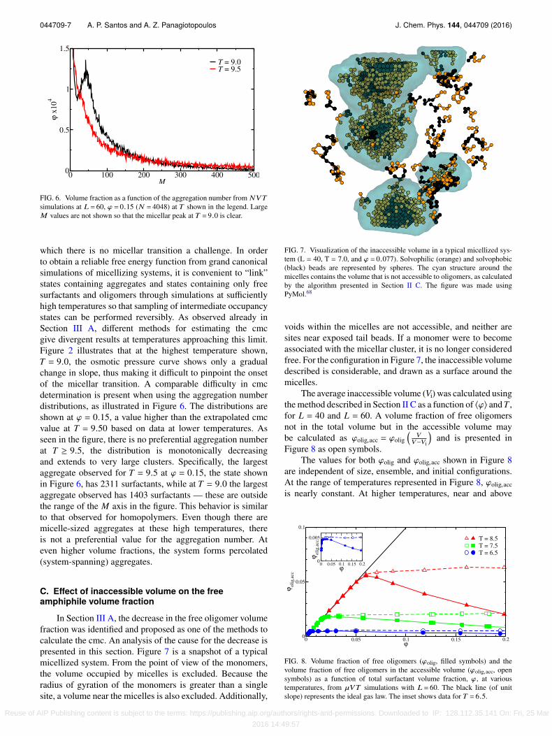
FIG. 6. Volume fraction as a function of the aggregation number from NVTsimulations at L = 60, ϕ = 0.15 (N = 4048) at T shown in the legend. LargeM values are not shown so that the micellar peak at T = 9.0 is clear.

which there is no micellar transition a challenge. In orderto obtain a reliable free energy function from grand canonicalsimulations of micellizing systems, it is convenient to “link”states containing aggregates and states containing only freesurfactants and oligomers through simulations at sufficientlyhigh temperatures so that sampling of intermediate occupancystates can be performed reversibly. As observed already inSection III A, different methods for estimating the cmcgive divergent results at temperatures approaching this limit.Figure 2 illustrates that at the highest temperature shown,T = 9.0, the osmotic pressure curve shows only a gradualchange in slope, thus making it difficult to pinpoint the onsetof the micellar transition. A comparable difficulty in cmcdetermination is present when using the aggregation numberdistributions, as illustrated in Figure 6. The distributions areshown at ϕ = 0.15, a value higher than the extrapolated cmcvalue at T = 9.50 based on data at lower temperatures. Asseen in the figure, there is no preferential aggregation numberat T ≥ 9.5, the distribution is monotonically decreasingand extends to very large clusters. Specifically, the largestaggregate observed for T = 9.5 at ϕ = 0.15, the state shownin Figure 6, has 2311 surfactants, while at T = 9.0 the largestaggregate observed has 1403 surfactants — these are outsidethe range of the M axis in the figure. This behavior is similarto that observed for homopolymers. Even though there aremicelle-sized aggregates at these high temperatures, thereis not a preferential value for the aggregation number. Ateven higher volume fractions, the system forms percolated(system-spanning) aggregates.

C. Effect of inaccessible volume on the freeamphiphile volume fraction

In Section III A, the decrease in the free oligomer volumefraction was identified and proposed as one of the methods tocalculate the cmc. An analysis of the cause for the decrease ispresented in this section. Figure 7 is a snapshot of a typicalmicellized system. From the point of view of the monomers,the volume occupied by micelles is excluded. Because theradius of gyration of the monomers is greater than a singlesite, a volume near the micelles is also excluded. Additionally,

FIG. 7. Visualization of the inaccessible volume in a typical micellized sys-tem (L = 40, T = 7.0, and ϕ = 0.077). Solvophilic (orange) and solvophobic(black) beads are represented by spheres. The cyan structure around themicelles contains the volume that is not accessible to oligomers, as calculatedby the algorithm presented in Section II C. The figure was made usingPyMol.68

voids within the micelles are not accessible, and neither aresites near exposed tail beads. If a monomer were to becomeassociated with the micellar cluster, it is no longer consideredfree. For the configuration in Figure 7, the inaccessible volumedescribed is considerable, and drawn as a surface around themicelles.

The average inaccessible volume (Vi) was calculated usingthe method described in Section II C as a function of ⟨ϕ⟩ and T ,for L = 40 and L = 60. A volume fraction of free oligomersnot in the total volume but in the accessible volume maybe calculated as ϕolig,acc = ϕolig

(V

V−Vi

)and is presented in

Figure 8 as open symbols.The values for both ϕolig and ϕolig,acc shown in Figure 8

are independent of size, ensemble, and initial configurations.At the range of temperatures represented in Figure 8, ϕolig,accis nearly constant. At higher temperatures, near and above

FIG. 8. Volume fraction of free oligomers (ϕolig, filled symbols) and thevolume fraction of free oligomers in the accessible volume (ϕolig,acc, opensymbols) as a function of total surfactant volume fraction, ϕ, at varioustemperatures, from µVT simulations with L = 60. The black line (of unitslope) represents the ideal gas law. The inset shows data for T = 6.5.

Reuse of AIP Publishing content is subject to the terms: https://publishing.aip.org/authors/rights-and-permissions. Downloaded to IP: 128.112.35.141 On: Fri, 25 Mar

2016 14:49:57

044709-8 A. P. Santos and A. Z. Panagiotopoulos J. Chem. Phys. 144, 044709 (2016)

the upper limit for micellization, ϕolig,acc follows the ideal-gastrend until percolation occurs. The constancy of ϕolig,acc abovethe cmc confirms the hypothesis that inaccessible volume isthe main cause for the observed decrease in ϕolig above thecmc.

There is a slight increase in the effect of inaccessiblevolume on ϕolig at higher temperatures, due to the change inthe size and shape of micelles as a function of ϕ and T . Atlow temperatures the micelles are large and dense, whereasat high temperature the solvent penetrates deeper into themicelle core. Micelles at higher temperature are more spreadout, thus increasing the amount of volume excluded explicitlyby surfactants in the micelles.

As stated already, the free oligomer or monomerconcentration from a single simulation at concentrationsabove the cmc is often used in simulations to provide anapproximation of the cmc. This has been shown earlier tobe a poor approximation for ionic surfactants.9,18–20 Here, weshow that this approximation can lead to significant errorsfor nonionic surfactants as well. For example, at T = 7.5,for an NVT simulation at ϕ = 0.0916 (approximately fivetimes ϕcmc), the uncorrected oligomer volume fraction isϕolig = 0.0146. However, the actual value is ϕcmc = 0.0182± 0.0005, as calculated by the maximum in the ϕolig, andϕcmc = 0.0178 ± 0.0006 from the osmotic pressure. Thus,ϕolig underestimates the true cmc by approximately 20%.Large-scale MD simulations of surfactants are often restrictedto concentrations much greater than the cmc, so thiscorrection needs to be taken into account for accurate cmccalculations.

IV. SUMMARY AND CONCLUSIONS

We have developed a method to calculate the volumemade inaccessible to free surfactants in micellar solutions.We show that the concentration of free surfactants in theaccessible volume is nearly constant above the cmc, whereasthe concentration of free surfactants in the total volumedecreases above the cmc. We thus conclude that, for nonionicsurfactants, the decrease in concentration of free surfactantsabove the cmc is due to the inaccessible volume. These volumeexclusion effects are not accounted for in mass-action-lawdescriptions of micellization. Because of the decrease infree surfactant concentration, simulation studies of nonionicsurfactants restricted to concentrations far above the cmc needto take into account the inaccessible volume to obtain accurateestimates for the cmc. The impact of the inaccessible volumeon ionic surfactants, for which solution ionic strength effectsalso come into play, will be the subject of future work.

Three methods for measuring cmc’s from simulationsof surfactant solutions were analyzed, namely through themaximum in the free oligomer concentration, the osmoticpressure of the solution obtained in grand canonical MonteCarlo simulations, and the presence of a minimum inthe aggregate size distributions between oligomeric andmicellar distributions. The maximum in the free oligomerconcentration, as mentioned, is a result of the inaccessiblevolume. Because micelles become more compact and smoothat low temperatures, the effect of the inaccessible volume

is less pronounced, and the maximum in the free oligomerconcentration is more difficult to identify. Additionally, at lowtemperatures it is more difficult to reach equilibrium, becauseof the significant barriers to surfactant transfer between freesolution and the interior of micelles. Reaching equilibriumat low temperature is also a challenge when calculating thecmc from a minimum in the aggregation number distributions,because these distributions cannot be reliably obtained. Bycontrast, cmc’s calculated from the osmotic pressure usinghistogram reweighting can be obtained from considerablyfewer simulations, using smaller system sizes. With fullyequilibrated histograms (which require simulations over arange of temperatures), the cmc at low temperature canbe reliably calculated. The main limitation of the osmoticpressure method is that it requires sampling in the grandcanonical ensemble, which may not be practical for explicit-solvent realistic surfactant models.

As the temperature increases the cmc definitions begin todeviate from each other, since micellar aggregates becomeless sharply defined and the aggregate size distributionsdevelop broad tails. These deviations signal the approachof an upper temperature limit above which micellization doesnot occur. This upper temperature limit for micellization canbe obtained from aggregation number distributions well abovethe extrapolated cmc. For the H4T4 surfactant, we find thatthis limit occurs approximately at T = 9.5.

ACKNOWLEDGMENTS

Financial support for this work has been provided by theDepartment of Energy, Office of Basic Energy Sciences, underAward No. DE-SC0002128. In addition, A.P.S. acknowledgesfunding from the National Science Foundation through aGraduate Research Fellowship.

1J. Israelachvili, Intermolecular and Surface Forces, 3rd ed. (Elsevier, Lon-don, 2011).

2A. González-Pérez, J. L. Del Castillo, J. Czapkiewicz, and J. R. Rodríguez,J. Chem. Eng. Data 46, 709 (2001).

3B. O. Persson, T. Drakenberg, and B. Lindman, J. Phys. Chem. 83, 3011(1979).

4C. Thévenot, B. Grassl, G. Bastiat, and W. Binana, Colloids Surf., A 252,105 (2005).

5J. van Stam, S. Depaemelaere, and F. C. De Schryver, J. Chem. Educ. 75, 93(1998).

6R. G. Alargova, I. I. Kochijashky, M. L. Sierra, and R. Zana, Langmuir 14,5412 (1998).

7T. Lazaridis, B. Mallik, and Y. Chen, J. Phys. Chem. B 109, 15098 (2005).8A. Vishnyakov, M.-T. Lee, and A. V. Neimark, J. Phys. Chem. Lett. 4, 797(2013).

9D. N. LeBard, B. G. Levine, P. Mertmann, S. A. Barr, A. Jusufi, S. Sanders,M. L. Klein, and A. Z. Panagiotopoulos, Soft Matter 8, 2385 (2012).

10M.-T. Lee, A. Vishnyakov, and A. V. Neimark, J. Phys. Chem. B 117, 10304(2013).

11A. Jusufi and A. Z. Panagiotopoulos, Langmuir 31, 3283 (2014).12F. H. Quina, P. M. Nassar, J. B. S. Bonilha, and B. L. Bales, J. Phys. Chem.

99, 17028 (1995).13B. L. Bales, J. Phys. Chem. B 105, 6798 (2001).14M. Benrraou, B. L. Bales, and R. Zana, J. Phys. Chem. B 107, 13432 (2003).15D. A. Amos, J. H. Markels, S. Lynn, and C. J. Radke, J. Phys. Chem. B 15,

2739 (1998).16D. W. Cheong and A. Z. Panagiotopoulos, Langmuir 22, 4076 (2006).17A. P. dos Santos, W. Figueiredo, and Y. Levin, Langmuir 30, 4593 (2014).18S. A. Sanders, M. Sammalkorpi, and A. Z. Panagiotopoulos, J. Phys.

Chem. B 116, 2430 (2012).

Reuse of AIP Publishing content is subject to the terms: https://publishing.aip.org/authors/rights-and-permissions. Downloaded to IP: 128.112.35.141 On: Fri, 25 Mar

2016 14:49:57

044709-9 A. P. Santos and A. Z. Panagiotopoulos J. Chem. Phys. 144, 044709 (2016)

19R. Mao, M.-T. Lee, A. Vishnyakov, and A. V. Neimark, J. Phys. Chem. B119, 11673 (2015).

20A. Jusufi, D. N. LeBard, B. G. Levine, and M. L. Klein, J. Phys. Chem. B116, 987 (2012).

21G. Gunnarsson, B. Joensson, and H. Wennerstroem, J. Phys. Chem. B 84,3114 (1980).

22A. Jusufi, Mol. Phys. 111, 3182 (2013).23E. A. G. Aniansson, S. N. Wall, M. Almgren, H. Hoffmann, I. Kielmann,

W. Ulbricht, R. Zana, J. Lang, and C. Tondre, J. Phys. Chem. 80, 905(1976).

24L. Maibaum, A. R. Dinner, and D. Chandler, J. Phys. Chem. B 108, 6778(2004).

25A. I. Rusanov, Langmuir 30, 14443 (2014).26J.-C. Desplat and C. M. Care, Mol. Phys. 87, 441 (1996).27A. D. Mackie, A. Z. Panagiotopoulos, and I. Szleifer, Langmuir 13, 5022

(1997).28M. Girardi and W. Figueiredo, J. Chem. Phys. 112, 4833 (2000).29M. Lsal, C. K. Hall, K. E. Gubbins, and A. Z. Panagiotopoulos, J. Chem.

Phys. 116, 1171 (2002).30H. W. Hatch, J. Mittal, and V. K. Shen, J. Chem. Phys. 142, 164901 (2015).31B. G. Levine, D. N. LeBard, R. DeVane, W. Shinoda, A. Kohlmeyer, and

M. L. Klein, J. Chem. Theory Comput. 7, 4135 (2011).32S. K. Talsania, Y. Wang, R. Rajagopalan, and K. K. Mohanty, J. Colloid

Interface Sci. 190, 92 (1997).33A. Ben-Naim and F. Stilllnger, J. Phys. Chem. 84, 2872 (1980).34E. Ruckenstein and R. Nagarajan, J. Phys. Chem. 79, 2622 (1975).35C. M. Wijmans and P. Linse, Langmuir 11, 3748 (1995).36J. N. B. de Moraes and W. Figueiredo, J. Chem. Phys. 110, 2264 (1999).37D. Attwood, P. H. Elworthy, and S. B. Kayne, J. Phys. Chem. 74, 3529

(1970).38D. Carrière, M. Page, M. Dubois, T. Zemb, H. Cölfen, A. Meister, L. Belloni,

M. Schönhoff, and H. Möhwald, Colloids Surf., A 303, 137 (2007).39M. A. Floriano, E. Caponetti, and A. Z. Panagiotopoulos, Langmuir 15, 3143

(1999).40A. Z. Panagiotopoulos, M. A. Floriano, and S. K. Kumar, Langmuir 18, 2940

(2002).41M. E. Gindy, R. K. Prud’homme, and A. Z. Panagiotopoulos, J. Chem. Phys.

128, 164906 (2008).42H. Bock and K. Gubbins, Phys. Rev. Lett. 92, 135701 (2004).

43S. Paula, W. Siis, J. Tuchtenhagen, and A. Blume, J. Phys. Chem. 99, 11742(1995).

44H.-U. Kim and K.-H. Lim, Colloids Surf., A 235, 121 (2004).45A. Couper, G. P. Gladden, and B. T. Ingram, Faraday Discuss. Chem. Soc.

59, 63 (1975).46P. R. Majhi and A. Blume, Langmuir 17, 3844 (2001).47G. C. Kresheck, J. Phys. Chem. B 102, 6596 (1998).48A. Jusufi, A.-P. Hynninen, and A. Z. Panagiotopoulos, J. Phys. Chem. B 112,

13783 (2008).49A. Jusufi, S. Sanders, M. L. Klein, and A. Z. Panagiotopoulos, J. Phys.

Chem. B 115, 990 (2011).50R. G. Larson, L. E. Scriven, and H. T. Davis, J. Chem. Phys. 83, 2411 (1985).51R. G. Larson, J. Chem. Phys. 96, 7904 (1992).52A. T. Bernardes, V. B. Henriques, and P. M. Bisch, J. Chem. Phys. 101, 645

(1994).53A. Bhattacharya and S. D. Mahanti, J. Phys.: Condens. Matter 13, L861

(2001).54S. Kim, A. Z. Panagiotopouolos, and M. A. Floriano, Mol. Phys. 100, 2213

(2002).55Z. A. Al-Anber, J. Bonet i Avalos, M. A. Floriano, and A. D. Mackie,

J. Chem. Phys. 118, 3816 (2003).56F. R. Siperstein and K. E. Gubbins, Langmuir 19, 2049 (2003).57A. G. Daful, J. B. Avalos, and A. D. Mackie, Langmuir 28, 3730 (2012).58A. Nikoubashman and A. Z. Panagiotopoulos, J. Chem. Phys. 141, 041101

(2014).59P. G. de Gennes, J. Chem. Phys. 55, 572 (1971).60D. Frenkel, G. Mooij, and B. Smit, J. Phys.: Condens. Matter 4, 3053 (1992).61A. Ferrenberg and R. Swendsen, Phys. Rev. Lett. 61, 2635 (1988).62M. J. Rosen and J. T. Kunjappu, Surfactants and Interfacial Phenomena, 4th

ed. (Wiley, New York, NY, 2012).63J. Hoshen and R. Kopelman, Phys. Rev. B 14, 3438 (1976).64M. N. Rosenbluth and A. W. Rosenbluth, J. Chem. Phys. 23, 356 (1955).65H. Flyvbjerg and H. G. Petersen, J. Chem. Phys. 91, 461 (1989).66A. Bhattacharya and S. D. Mahanti, J. Phys.: Condens. Matter 12, 6141

(2000).67P. Carpena, J. Aguiar, P. Bernaola-Galvan, and C. Carnero Ruiz, Langmuir

18, 6054 (2002).68The PyMOL Molecular Graphics System, Version 1.3r, Schrödinger, LLC,

2010.

Reuse of AIP Publishing content is subject to the terms: https://publishing.aip.org/authors/rights-and-permissions. Downloaded to IP: 128.112.35.141 On: Fri, 25 Mar

2016 14:49:57