DETERMINANTS OF SWAZILAND MANUFACTURING OUTPUT – …mefmi.org/mefmifellows/wp-content/uploads/2016/10/DETERMINANTS-OF...coefficient for foreign demand, proxied by manufactured good

DETERMINANTS OF SWAZILAND MANUFACTURING OUTPUT – SUPPLY AND

DEMAND APPROACHES

A TECHNICAL PAPER SUBMITTED IN FULFILMENT OF MEFMI FELLOWSHIP PROGRAMME:

BY:

PATRICK NDZINISA1

THE CENTRAL BANK OF SWAZILAND, RESEARCH

DEPARTMENT

MAY, 2007

1 Patrick Ndzinisa, Central Bank of Swaziland, Box 546 Mbabane, Swaziland, Tel: (268) 408 2204, Fax: (268) 404 0038, E-mail: [email protected]

ii

TABLE OF CONTENTS

Acknowledgements…………………………………………………..…………(iii)

Abstract…………………………………………………………………….….….(iv)

1. INTRODUCTION……………………………………………………………….…...1 2. OVERVIEW OF THE SWAZILAND ECONOMIC STRUCTURE……………...3

2.1 Manufacturing Sector……………………………………………………...3

2.2 Agricultural Sector…………………………………………………….……4

2.3 Other Sector…………………………………………………………..…….5 3. LITERATURE REVIEW…………………………………………….……………...7 4. DATA DESCRIPTION AND SOURCES………………………………………..11 5. METHODOLOGY…………………………………….………………………...…12

5.1 Specification of the equations……………………………………….…..12

5.2 Stationarity…………………………………………………………….…..13

5.3 Cointegration and Error Correction Model (ECM)…………………….14

5.4 Diagnostic Tests…………………………………………………………..16 6. EMPIRICAL RESULTS………………………………………………………......17

6.1 Stationarity and Cointegration Test Results…………………………...17

6.2 Diagnostic Test Results………………………………………………….18

6.3 Estimation Results and Interpretations…………………………………18 7. CONCLUSIONS AND POLICY IMPLICATIONS…………………………..….21

APPENDIX A ……………………………………………………………………………....23

APPENDIX B…..........................................................................................................24

APPENDIX C…………………………………………………………………………….....25

APPENDIX D…………………………………………………………………………...…. 26

APPENDIX E……………………………………………………………………………….27

APPENDIX ………………………………………………………………………………..28

APPENDIX G……………………………………………………………………………….29

APPENDIX H……………………………………………………………………………….30

APPENDIX I………………………………………………………………………..……….31

REFERENCES………………………………………………………………………….….32

iii

ACKNOWLEDGEMENTS

I am greatly indebted to my mentor Theo Janse van Rensburg. He acted as a

furnace, helping to refine rough ideas and to focus the study. Without his

guidance and patience, this paper would not have been a success.

I am also grateful to MEFMI and the Central Bank of Swaziland, not only for

their financial assistance without which I would not have been able to attend

the relevant courses, but also for providing guidance and support. I am

particularly grateful for the generous time that the Central Bank of Swaziland

has granted me to complete this paper.

I am also indebted to the Research Staff of the Central Bank of Swaziland,

particularly Andreas Dlamini and Vusi Khumalo who assisted me with various

data issues - particularly during my visit to the South African National

Treasury in April 2007.

Lastly, but not least, I am thankful to my family for their understanding and

moral support throughout the study, but in particular during the period of the

MEFMI Customized Training Programme (CTP).

iv

ABSTRACT

The paper analyzed the determinants of the manufacturing output in Swaziland

from a supply and demand perspective. The results from the supply equation

confirmed the relative importance of both human- and physical capital. The

study also confirmed the strong linkage between agricultural- and

manufacturing output, indicating an elasticity of manufacturing production

with regard to agricultural output of +0.43

Meanwhile the demand equation also emphasized the importance of both

foreign and domestic demand in determining manufacturing output. The

coefficient for foreign demand, proxied by manufactured good exports,

signified the reliance of the Swazi economy, particularly manufacturing output,

on export for growth. It has been also observed that whilst FDI positively and

significantly affects manufacturing output it does so in the short-run. The

absence of long run FDI benefits is surprising, but may reflect unique

Swaziland circumstances, where FDI in the 1980’s was largely in response to

sanctions imposed on its neighbor, South Africa.

The paper thus argues that in the light of Swaziland’s manufacturing

dependence on the agricultural sector, the country should institute policy

measures to enlarge and diversify its economic base; there is a need to invest

in human capital in order to complement the increase in physical capital; the

country should pursue vigorous strategies through SIPA in order to promote

FDIs with long term benefits, hence manufacturing output growth. Economic

policy should encourage a competitive environment. In this regard sound

monetary and fiscal policies aimed at inflation stability will play an important

role.

1

DETERMINANTS OF SWAZILAND MANUFACTURING OUTPUT –

SUPPLY AND DEMAND APPROACHES

1. INTRODUCTION

Swaziland is a tiny land-locked country with small domestic markets. The

economy of Swaziland is heavily dependent on exports, largely based on

agricultural production and agro-processing manufacturing industries.

Although agricultural production constitutes less than 10 per cent of GDP, the

sector plays a significant role in determining the country’s economic growth

and development through its many forward- and backward linkages with other

sectors. Although other sectors (with 2004 GDP share in brackets) such as

manufacturing (34.8%), government services (16.6%), wholesale, retail,

hotels and restaurants (12.8%) also play an important role, variations in

overall output is largely related to changes in agricultural output and its

linkages to other sectors, in particular manufacturing. For instance, the recent

sluggishness in real economic growth is primarily attributed to reduced

agricultural production and the consequent slowdown in agro-processing in

the manufacturing sector. Given the revised estimated population growth rate

of 2 percent2, the slow economic growth has failed to achieve the desired

improvement in living standards. In fact the standard of living as measured by

per capita income has been falling since 19913. This is contrary to the

government’s objective of alleviating poverty in the country.

During the 1980s Swaziland recorded high economic growth rates, driven by

an influx of foreign direct investment (FDI) arising from sanctions imposed on

South Africa, which propelled the relocations of enterprises into Swaziland.

The high levels of foreign direct investment caused an economic upturn in the

2 Given government’s vision to reduce poverty rate by 50 percent by 2015 coupled with the assumed population growth rate of 2.75 percent, a minimum annual economic growth rate of 5 percent is required in order also to accommodate the resultant growth in labor force. 3 GDP per capita are published in the Central Bank of Swaziland’s quarterly review bulletin

2

manufacturing sector, which became the main growth engine, which in turn

encouraged rapid growth in supporting sectors such as construction as well

as generating additional revenue which permitted the consequent expansion

of government services. Apart from the inflows into the manufacturing sector,

the growth performance was also aided by more conventional external stimuli,

such as improved export prices for sugar, reinforced by the real depreciation

of the lilangeni.

However, since the 1990s the pace of economic growth has been falling

substantially when compared to rates achieved during the 1980s (see graph 1

in appendix B). GDP growth averaged 6.7 percent during the 1980s before

declining to an average of 3.2 percent in the 1990s and to around 2.6 percent

during the period 2000 to 2004. Given the economy’s dependence on agro-

processed goods for growth, the observed decline in the growth rate

symbolises a similar trend in the manufacturing and agricultural sectors.

These sectors have been adversely affected by, among other factors, the

slowdown in investment inflows due to stiff competition for foreign investment

in the region, particularly as the political and business environment improved

in the region. This was aggravated by fluctuations in international commodity

prices and the exchange rate, as well as unfavourable weather conditions and

the consequent closure of some major companies.

Chart 1 in appendix B compares Swaziland’s economic growth with selected

SADC countries. Whilst a majority of the SADC countries recorded economic

growth in excess of 3 percent, Swaziland’s economic growth was hovering

below that level. Countries like Botswana and Mozambique continue to

experience strong GDP growth due to the continued expansion of the mining

sector in Botswana and the significant expansion of the manufacturing and

telecommunications sectors in Mozambique.

3

Given the direct linkage between the manufacturing sector and the

agricultural sector in Swaziland, any growth strategy should take these

linkages into account. This study econometrically confirms the above

observations and also indicates that the elasticity of manufacturing production

with regard to agricultural output is +0.43. The main objective of the study

therefore is to identify factors that drive manufacturing output both from a

supply and demand perspective.

The rest of the paper is structured as follows. Section 2 of the paper gives an

overview of the structure of the Swazi economy with emphases on the

manufacturing- and agricultural sectors. In section 3 a literature review on the

determinants of economic growth with particularly emphasis on the

manufacturing sector is presented. Section 4 gives an overview of the data

and the sources, whilst the estimation methodology is discussed in section 5.

In section 6 the estimation results is presented, followed by conclusions and

policy implications in the final section of the paper.

2. OVERVIEW OF THE SWAZILAND ECONOMIC STRUCTURE

2.1 MANUFACTURING SECTOR

Most of the industries are foreign-owned, export-oriented and have strong

backward and forward linkages with agriculture. Manufacturing industries

range from small factories engaged in light industry to large ones endowed

with the latest technology and producing highly sophisticated goods which,

given the small size of the domestic market, are destined mainly for the

export market. The major export commodities produced are wood products,

soft drink concentrates, canned fruits, sugar, and mineral products. The

sector’s share of overall output declined slightly from 35.8 percent in 2000 to

34.8 percent in 2004. The sector’s contribution to employment creation has

declined in recent years as firms raised their capital intensity in the production

process. However, new medium and large scale enterprises, which tend to be

more labour intensive has ventured into yarn production and wheat milling, as

4

well as the manufacturing of items such as refrigerators and knitwear.

Although there has been a move towards manufacturing diversification, this

trend needs to be intensified in order to create significantly more formal sector

employment.

The major constraints to further development of the manufacturing sector

include the small size of the domestic market and the relatively narrow

resource base. Inadequate infrastructure also continues to present a major

barrier to output growth. In order to improve the investment climate,

Government has given high priority to enhancing the availability of physical

infrastructure in transport and communications, and also to increase the

number of skilled personnel in management and engineering. Government is

also pursuing a wage policy that matches real remuneration growth with

increases in labour productivity.

However, future prospects of the manufacturing sector depends on the

country’s ability to retain the preferential trade treatment under the introduced

African Growth and Opportunity Act/Trade and Development Act of 2000,

which introduced a new co-operation agreement between the United States

and eligible sub-Saharan countries. Not only does this legislation represents a

solid, meaningful, and significant opportunity, but is also likely to result in

substantial new trade and investment flows between the US and Africa.

2.2 AGRICULTURAL SECTOR

The agricultural sector, which consists of the traditional and modern sub-

sectors, plays a pivotal role in Swaziland’s economy. Despite the declining

volumes of output, the agricultural sector remains indispensable for the

majority of Swazi people who continue to derive their livelihood and income

by engaging in this sector’s activities, which include the production of maize,

cotton, sugar, fruits, vegetables, citrus and livestock. Moreover, the

agricultural sector plays an important role in providing substantial support to

5

the manufacturing sector, in terms of intermediate inputs required by the

largely agro-based manufacturing companies producing manufactured goods

such as wood-pulp, sugar-based edible concentrates and blends, sugar,

canned fruits, sweets and other edible commodities.

The agricultural sector, particularly traditional agriculture, is constrained by

several factors, such as inadequate credit facilities, poor storage facilities and

marketing services and inappropriate pricing policies and low livestock off-

take, exacerbated by soil erosion. The overall performance of the agricultural

sector marginally improved in 2004 as real value added increased by 0.2

percent. Table 1 in appendix A reveals that as a share of GDP, the

agricultural sector contributed 8.8 percent to overall economic activity,

compared to 8.6 percent in the previous year. The sector is the main source

of livelihood for over 70% of the population and is the primary source of

employment and income for rural households.

2.3 OTHER SECTORS

The other sectors of the Swaziland economy comprise; construction,

transport and communications, Banking and insurance etc (see table 1 of

appendix A for each sector’s relative GDP contribution).

Construction Sector: The level of activity in the construction sector is largely

related to overall economic activity. As firms set up or expand operations,

they require new factories and accommodation for the additional workers.

Likewise an expansion of the trade sector would encourage the building of

new shopping centers. Once these facilities are complete, construction

activity declines and the sectoral contribution falls. For the construction sector

to play a meaningful role, overall economic growth would need to be

accelerated significantly on a sustainable basis.

6

Wholesale, Retail, Hotels and Restaurants Sector: Swaziland has a well-

developed retail and wholesale sector, which is dominated by branches of the

leading South African chain stores. With the legalisation of casinos in SA, and

increased competition for South African tourists emanating from the growing

Mozambican tourism industry, the sector's growth rate has declined in recent

years.

Transportation and Communications: The transport system constitutes a

vital service sector of the Swazi economy. This sector has continued to grow

strongly and has become the second most significant sector in secondary

production. The road network constitutes the most predominant mode for

transport of people and goods. The airport can accommodate medium-sized

jet aircraft. The railway infrastructure provides an important regional link from

countries to the north to the ports of Durban and Richards Bay in South

Africa. The Kingdom’s telephone network is fully digital. Since its inception in

1998, Swazi MTN has significantly developed the cellular network, and now

provides in excess of 80 percent coverage of the country’s geographical area.

So far it distributes its products through its service centres in Manzini and

Mbabane as well as its distribution network with some retail outlets

strategically situated throughout the country. The Internet system has become

an integral part of the communications network in Swaziland with both

organisations and individuals linking onto the international network.

Banking and Insurance Sector: Swaziland’s financial sector comprises the

Central Bank of Swaziland, three locally incorporated banks, a development

bank, one building society and other financial institutions. In the development

of the country’s financial sector, the Ministry of Finance works very closely

with the Economic Planning and Development Ministries and the Central

Bank.

7

The Ministry of Finance is charged with the responsibility of managing the

fiscus, whilst the Central Bank of Swaziland’s objective is to contribute to the

country’s economic growth through promotion of monetary stability and by

fostering an environment which ensures a stable and sound financial system.

Given its membership in the CMA, Swaziland has little scope for independent

monetary policy to influence the price level. Given the fixed exchange rate

system with South Africa, the rate of inflation in Swaziland is largely a

reflection of SA inflation.

3. LITERATURE REVIEW

This section presents a brief overview of economic growth theories and

empirical evidence regarding the linkages between macroeconomic variables

and manufacturing growth in different countries.

The evolution of economic growth theories have culminated in modern growth

theory, dating back to the 1960s. The earliest study was conducted by Solow

and Swan (1956) based on neoclassical economic theory. The underlying

assumptions of neo-classical growth theory are; a single homogeneous good,

exogenous labor-augmenting technical progress, full employment and

exogenous labour force growth.

The assumptions imply that in steady-state equilibrium, the level of GDP per

capita will be determined by the prevailing technology and the exogenous

rates of saving, population growth and technical progress. Solow and Swan

concluded that different saving rates and population growth rates might affect

different countries’ steady-state levels of per capita income. That is, other

things being equal, countries that have higher saving rates tend to have

higher levels of per capita income, and vice versa. The starting point of

empirical growth models is the neoclassical production function:

( ) ( , )1 Y A F K Lt t t t

8

Where Y = total output, L, K – capital and labour inputs respectively, and A =

autonomous technical change.

Neoclassical theory argues that sustained growth occurs through an

exogenous factor of production. It relates output to factor inputs, which

consist of the stock of accumulated physical capital goods and labour, which

is regarded as only one type (De Jager 2004). According to the theory the

production function exhibits decreasing returns with respect to each factor of

production whilst keeping the other constant. This implies that an increase in

the stock of capital whilst keeping labour constant will result in a less than

proportionate increase in output. Additional capital will ultimately produce no

additional output symbolising zero growth. The most important shortcoming of

this model, at least from the point of view of developing countries, is that there

is limited scope for policies to influence the rate of growth of output in the

steady state. This is the case because in the steady state higher savings or

investments, which are very low in developing countries, are required for the

economy to grow, hence reach a new steady state. (Mankiw, 2003)

Due to these shortcomings, recent growth models dismiss the Solow-Swan

model in favor of an endogenous growth model that assumes constant and

increasing returns to capital. Two main streams of endogenous growth

theories have emerged, namely those focused on technological change and

those mainly concerned with human capital. Whilst the traditional growth

theory emphasized the two factors of production, that is capital and labour,

new growth theory adds a third factor, technology. The incorporation of the

concept of technology as a factor of production necessitates a different set of

institutional arrangements, like pricing systems, taxation or incentives to

ensure the efficient allocation of ideas. Endogenous growth theory with

human capital puts more emphasis on human knowledge as an underlying

factor to the production function as it accumulates over time. Arrow (1962:

157) devised a model of learning-by-doing, which shows that experience in

9

production, results in higher productivity and economic growth. Given that

experience is not measurable, Arrow considered cumulative gross investment

as a proxy for experience by arguing that each new piece of machinery

produced and put in use, is capable of changing the environment in which

production take place, so that learning is taking place with continuous new

stimuli.

Studies on manufacturing output growth from the supply perspective have

also emphasized the importance of both physical and human capital, labour

and technological progress as the main drivers of the sector’s growth. In a

study on “Supply and demand of manufacturing output in OECD countries

1970-95” by Cancelo, Guisan and Frias (2001), manufacturing output is

expressed as a function of industrial employment, the stock of industrial

capital and R & D expenditure to proxy the influence of technological

activities. As expected, the study indicated a positive relationship between

each of the three explanatory variables and manufacturing output. The

elasticity of capital stock was the largest, thus highlighting the importance of

investment in explaining variations in manufacturing output in the OECD

countries.

Miao Grace Wang (2003) in his study on the impact of foreign direct

investment (FDI) inflows on a host country’s economic growth (evidence from

Asian countries) observed that although total FDI inflows in these countries

contribute positively on the economic growth, not all sector’s FDI inflows are

important. The results of the study indicated that FDI in the manufacturing

sector has a significant and positive effect on economic growth in the host

country whilst FDI in the non-manufacturing sectors do not play a significant

role in enhancing economic growth. The study indicated that a one

percentage point increase in manufacturing FDI leads to a 1.0823 percentage

point increase in per capita real GDP growth. This emphasizes the

importance of FDI inflows in the manufacturing sector as a potentially major

10

engine of growth for developing countries through its positive impact on

manufacturing growth and ultimately overall economic growth. It is often

postulated that FDI from developed countries to developing countries is a

vehicle not only for providing physical capital, but also for transferring

advanced technology, managerial skill, and innovative products.

In the Miao Grace Wang (2003) study, human capital was proxied by the

average number of years in secondary and higher education for the male

population in each country. Similarly a study by Ben Habib and Speegel

(1994) revealed a significant and positive relationship between human capital

and total factor productivity. Research on Tanzania has also indicated that

that the small manufacturing enterprises with more educated and trained

entrepreneurs are more productive in generating output and demand for

labour than their less educated or trained counterparts (D. Mahadea and A.

Mkocha (2003)).

Manhal M. Shotar and Walled Hmedat (2003) have discovered a positive and

significant impact between intermediate good imports and manufacturing

output.

The broad consensus highlighted in these studies is that a country’s

manufacturing growth over the long term is determined by mainly three

factors, namely the efficient utilisation of the existing stock of both human and

physical capital as well as technological progress. This may be supplemented

by factors such as FDI flows and intermediate good imports by the

manufacturing sector.

Cancelo, Guisan and Frias (2001) also investigated manufacturing output

from a demand perspective. The paper concluded that demand for

manufacturing output in the OECD countries is explained by, amongst other

factors, domestic and foreign demand, manufacturing imports and relative

11

prices. In this paper, foreign demand was proxied by manufacturing exports

from each country to the OECD, whilst domestic demand was proxied by

each country’s GDP, lagged by one period. Relative prices depicted a

negative sign, thus confirming structural competitiveness. Although the study

found an unexpected positive sign with respect to the manufacturing imports

variable, the authors indicated that manufacturing imports could be acting as

a proxy for the consumption of intermediate inputs in manufacturing

production.

4. DATA DESCRIPTION AND SOURCES

The study is based on time series data. The econometric implication of the

models specified in equations (5.1.1) and (5.1.2) required time series data on

the following variables: real agriculture gross domestic product; real

manufacturing gross domestic product; real manufacturing capital stock;

number of people employed in the manufacturing sector; real expenditure on

education (a proxy for human capital); real gross domestic product; the real

effective exchange rate of the lilangeni against trading partners; real

manufacturing exports (a proxy for foreign demand in equation (5.1.2)); Real

manufacturing imports; real prime interest rate and real foreign direct

investment by the manufacturing sector. Due to data unavailability for some

data series the study had to be limited to the period 1980 – 2004.

The data has been obtained from various sources, i.e. the Central Statistical

Office (CSO), Ministry of Enterprises and Employment (MoEE), the Central

Bank of Swaziland’s (CBS) publications, IFS and WDI data bank. Where

needed, nominal variables were deflated into real values using the GDP

deflator as compiled by the CSO. See table 2 in appendix A for a list of the

variables and the data sources.

12

5. METHODOLOGY

5.1 SPECIFICATION OF THE EQUATIONS

International literature indicates (see section 3) that by following a supply

specification, manufacturing output is determined by both physical and human

capital. As a measure of human capital the study uses education spending.

Given also the unique characteristics of the Swaziland manufacturing sector

(see paragraph 1 of section 1), agricultural output is added as an additional

explanatory variable. Consequently, the real value added in manufacturing

sector can be specified as follows:

)1.1.5.......(..............................................................................................................

)log()log()log(Re)log()log( 43210

EmanRagrducRcapRman

Where:

Rman = real manufacturing output;

Rcap = the real capital stock;

Reduc = the real expenditure on education a proxy for human capital.

Eman = the number of persons employed by the manufacturing sector;

Ragr = real added value of the agricultural sector to take into account the

effect of agriculture on the manufacturing sector and

µ = the error term.

From a demand perspective, manufacturing output can be expressed as

follows (also see section 3):

)2.1.5...(......................................................................)_log()(

)log()log(Reexp)log()log()log(

65

43210

mRfdiRpr

RmanfimperRmanRgdpRman

Where:

Rman = as defined in equation 5.1.1

Rgdp = the real domestic GDP a proxy for domestic demand

13

Rmanexp = the real manufacturing export a proxy for foreign demand

Reer = the real effective exchange rate of the lilangeni against trading

partners’ currencies a proxy for relative price

Rmanfimp = real manufacturing imports

Rpr = the real prime interest rate

Rfdi_m = real manufacturing foreign direct investment

ε = the error term.

The above equation specifications was adjusted to reflect the appropriate

single equation estimation techniques (see equation 5.3.1 below), using E-

Views software. The estimated equations were subjected to a battery of

econometric tests to ensure that an efficient and correctly specified model

was estimated.

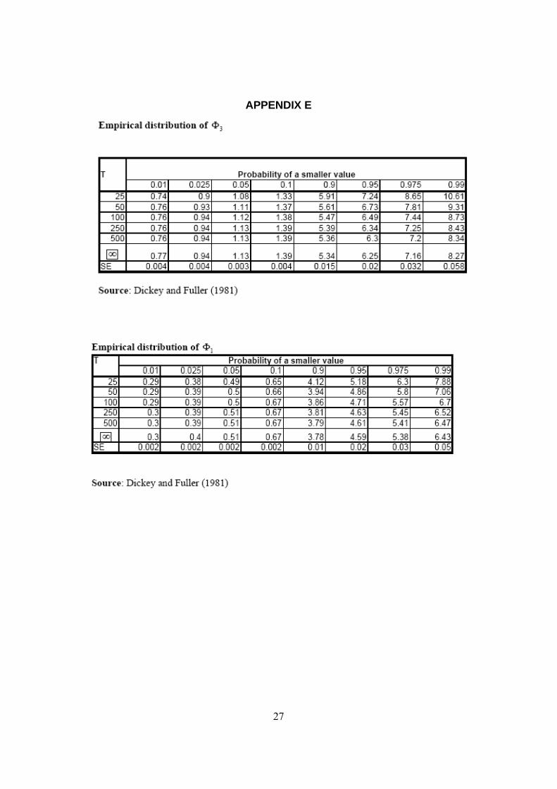
5.2 STATIONARITY

Time series data tend to exhibit a stochastic or deterministic trend with the

mean, variance and covariance changing over time, and thereby rendering

the series non-stationary. The first step is thus testing for stationarity for each

individual data series before estimating the equations. The null hypothesis of

non-stationarity of the variables is tested against the alternative hypothesis of

stationarity using the augmented Dickey-Fuller (ADF)-(Dickey-Fuller (1979)).

The ADF test establishes the data generating process (DGP) from the

following:

Pure random walk

Random with drift/constant

Random walk with drift and time trend

The ADF test for stationary is based on the following equation:

14

tit

n

iitt YYTY

21 ………………………………………….5.2.1

Where Y is the series tested for stationarity, i ,,, are parameters and εt

is white noise. The ADT test can be summarised as below.

Table2 Summary of the ADF Tests

Model Hypotheses Test Statistic

Random walk with drift and time trend

tit

n

iitt YYTY

21 H0: ρ=0, H1: ρ<0 τ τ

H0: ρ= λ=0, H1: ρ ≠0 and λ ≠0, Φ3

ρ =0 and λ ≠0, ρ≠ 0 and λ =0

Random walk with drift

tit

n

iitt YYY

21 H0: ρ=0, H1: ρ<0 τμ

H0: ρ= μ=0, H1: ρ ≠0 and μ ≠0, Φ1

ρ =0 and μ ≠0, ρ≠ 0 and μ =0

Pure random walk

tit

n

iitt YYY

21 H0: ρ=0, H1: ρ<0 τ

5.3 COINTEGRATION AND ERROR CORRECTION MODEL (ECM)

The consequence of working with non-stationary data series in the estimation

process is that this may yield a meaningless or spurious result, that is, there

is danger of obtaining apparently significant regression results from unrelated

data.

If non-stationary time series are used in regression models there is a need to

test further for cointegration amongst the series. Testing whether y and x

(which have been both generated by I(1) time series processes) are

15

cointegrated an Engle and Granger (1987) two-step procedure is widely used.

Johansen (1988) also proposed a general framework for testing

cointegration4. The Engle and Granger test for cointegration is often referred

to as the residual based test which the study uses based on the assumption

that there is only one cointegrating vector in the equations. The presence of a

cointegrating relationship allows us not only to estimate the long-run

relationship but also to further analyze the short-run dynamics and how

adjustment to equilibrium is achieved. Therefore according to the Granger

representation theorem, the existence of a stable long-run relationship

between the variables enables us to estimate an ECM.

Error correction models are based on the behavioral assumption that two or

more time series exhibit an equilibrium relationship that determines both

short- and long-run behavior. ECMs are useful as they reconcile the short-

and long-run behavior of the variables by shedding light on the speed or rate

of adjustment towards long-run stable equilibrium. Two different econometric

methodologies can be used in the construction of the ECM namely the

generalized one-step procedure5, and Engle and Granger two-step

procedure. The single-equation generalized error correction model (GECM)

has proven to be both theoretically appealing and also statistically superior to

the two-step estimator by Engle and Granger (1987) in many cases (Suzana

De Boef, 2000); hence the study uses the one-step method.

Given the long-run relationship between Y and X as ttt XY 21 the

GECM is estimated in one step as follows:

4The Johansen test is preferred when there are more than two time series variables involved because it can determine the number of cointegrating vectors 5The one-step error correction model, which was popularized by Davidson et al. (1978), is a transformation of an autoregressive distributed lag (ADL) model (Banerjee et al. 1993). Unlike the Engle and Granger Two-Step Method where the error term incorporated in the ECM is derived from a long-run equation, the one-step method estimate the error correction coefficient directly from a single equation containing both long- and short-run variables, rather than deriving it from alternative specifications (Suzanna De Boef 2000)

16

tttt XYXYY 51431211 .................................................(5.3.1)

Where Δ is the first difference, λ1 is the coefficient of adjustment to

equilibrium. Theory predicts that the adjustment term must be negative and

significantly different from zero. A negative λ1 implies that in the event of a

deviation between the short-run and the long-run equilibrium, there would be

an adjustment back to the long-run (stable) relationship in subsequent periods

to eliminate this discrepancy.

5.4 DIAGNOSTIC TESTS

The following diagnostic tests were conducted to establish the robustness of

the estimation results:

DIAGNOSTIC TESTS

Test Testing For

Jarque-Bera - Bera, Anil K.; Carlos M.

Jarque (1980).

Normality

ARCH White - White, Halbert (1980) Heteroscedasticity

Breuch-Godfrey LM Test - Breuch T.S;

Godfrey L.G. (1978)

Serial Correlation

Chow Forecast Test – Gregory C.

Chow (1960)

Recursive Coefficients (visual Test)-

Banerjee et al. (1992)

Stability

17

6. EMPIRICAL RESULTS

6.1 STATIONARITY AND COINTERGRATION TEST RESULTS

As discussed in the methodology section each of the variables used in the

two equations was tested for stationary. Said and Dickey (1984) suggested a

maximum number of lags of INT(N1/3) i.e. an integer of (N1/3), where N is the

number of observations. With 25 observations the maximum number of lags

would INT(251/3) ≈ 3. The stationarity and cointegration tests are shown in the

table below.

Variables T.Tests Conclusion

τ τ Φ3 τμ Φ1 τ

RMAN -1.885811 6.857368 -1.145391 9.650499 0.611415 I(1)

RAGR -2.309840 1.159124 -2.668636 0.725078 0.247972 I(1)

EMAN -3.019335 0.400185 -0.342890 0.915426 0.795101 I(1)

REDUC -2.055358 5.179123 -0.897742 3.197823 1.300032 I(1)

RCAP -2.541061 0.908947 -0.588490 1.121999 -1.517032 I(1)

RGDP -2.232310 2.199262 -0.382996 3.999524 2.001793 I(1)

REER -3.715301 0.544950 -1.546718 1.537182 0.596975 I(1)

RMANEXP -3.524719 0.211732 1.035377 -0.431504 1.318223 I(1)

RMANFIMP -3.029670 0.833812 -1.739495 0.097657 -0.469969 I(1)

RPR -4.198106** 0.124140 -3.405651 0.118259 -2.274104** I(0)

RFDI_M -2.612087 1.291150 -0.639452 2.471520 0.883807 I(1)

RESID_RMANDEM -4.402451*** I(0)

RESID_RMANSUP -4.418722*** I(0)

Note: *, ** and *** denotes significance at 10%, 5% and 1% respectively for t values. However, for the F statistics i.e. for Φ3 and Φ1: *, ** and ***represent significance at 95%, 97.5% and 99% confidence intervals respectively. Otherwise not significant hence the null hypotheses that the variable has a unit root cannot be rejected.

The stationarity test results indicate that all the variables, with the exception

of the real prime are integrated of order one, i.e. I(1). The residual terms for

the demand and supply equations (i.e. RESID_RMANDEM and

RESID_RMANSUP) are stationary, implying a cointegrating relationship in

each of the two estimated equations.

18

6.2 DIAGNOSTIC TESTS RESULTS

The various diagnostic tests results are reflected in the tables below.

TABLE 6.2.1 Supply Equation

Normality JB(2) =0.808 [0.668] Serial correlation LM(3) = 2.887 [0.070 Heteroscedasticity ARCH(-1) = 0.308 [0.584] Stability Test Chow Forecast = 4.240 [0.130] TABLE 6.2.2 Demand Equation

Normality JB(2) =1.603 [0.449] Serial correlation LM(2) = 0.876 [0.440] Heteroscedasticity ARCH(-1) = 0.050 [0.826] Stability Test Chow Forecast = 2.888 [0.286]

The diagnostics tests were conducted on the ECM specification of the supply

and demand equations and the results are depicted in tables 6.2.1 and 6.2.2

respectively. The results indicate that the errors of the two equations are

normally distributed and that there is no serial correlation in either of the two

equations at the 5 percent level. Similarly the ARCH test results indicate that

there is no presence of heteroscedasticity in the estimated equations. Finally

both the Chow Forecast test and the visual test (recursive coefficients)6

stability tests indicated that the parameters of the models are stable.

6.3 ESTIMATION RESULTS AND INTERPRETATIONS

The estimation results of the supply and demand equations are presented in

appendix C and D respectively. The findings of the study are in line with

earlier empirical studies.

With respect to the recent empirical literature, the supply equation results

confirm the relative importance of both human and physical capital in

determining manufacturing output in Swaziland. Assuming a constant returns

6 For the visual test results see appendix H and I

19

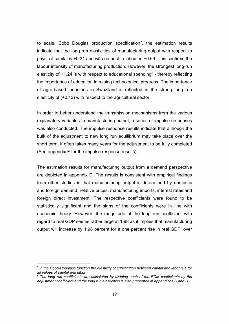
to scale, Cobb Douglas production specification7, the estimation results

indicate that the long run elasticities of manufacturing output with respect to

physical capital is +0.31 and with respect to labour is +0.69. This confirms the

labour intensity of manufacturing production. However, the strongest long-run

elasticity of +1.24 is with respect to educational spending8 - thereby reflecting

the importance of education in raising technological progress. The importance

of agro-based industries in Swaziland is reflected in the strong long run

elasticity of (+0.43) with respect to the agricultural sector.

In order to better understand the transmission mechanisms from the various

explanatory variables to manufacturing output, a series of impulse responses

was also conducted. The impulse response results indicate that although the

bulk of the adjustment to new long run equilibrium may take place over the

short term, if often takes many years for the adjustment to be fully completed

(See appendix F for the impulse response results).

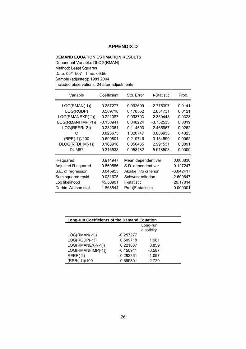
The estimation results for manufacturing output from a demand perspective

are depicted in appendix D. The results is consistent with empirical findings

from other studies in that manufacturing output is determined by domestic

and foreign demand, relative prices, manufacturing imports, interest rates and

foreign direct investment. The respective coefficients were found to be

statistically significant and the signs of the coefficients were in line with

economic theory. However, the magnitude of the long run coefficient with

regard to real GDP seems rather large at 1.98 as it implies that manufacturing

output will increase by 1.98 percent for a one percent rise in real GDP, over

7 In the Cobb-Douglass function the elasticity of substitution between capital and labor is 1 for all values of capital and labor 8 The long run coefficients are calculated by dividing each of the ECM coefficients by the adjustment coefficient and the long run elasticities is also presented in appendices C and D

20

the long term. This strong coefficient is puzzling given that the bulk of

Swaziland manufactured production is destined for export markets9.

Foreign demand was proxied by manufactured exports. The high long-run

elasticity of +0.86 implies that a one percent increase in manufactured

exports should raise manufacturing output by 0.86 percent over the long run.

This re-emphasises the dependence of the Swazi economy (particularly the

manufacturing sector) on exports for growth. The real effective exchange rate

and the manufacturing imports variables have the expected signs and are

statistically significant. The estimated equation indicates that manufacturing

output is highly sensitive to exchange rate developments, i.e. a one percent

decrease in the real effective exchange rate will increase manufacturing

output by 1.1 percent over the long run.

As expected, the elasticities with regard to manufacturing imports and the real

prime lending rate were found to be negative. The (-0.59) long-run elasticity of

manufacturing imports implies that a one percent increase in manufacturing

imports should lower manufacturing output by 0.59 percent over the long run.

The estimation results also indicate that a one percent increase in the real

prime lending rate will lower manufacturing output by 2.72 percent over the

long-run, reflecting the sensitivity of manufacturing output to changes in the

user cost of capital in Swaziland.

The study also found that although foreign direct investment has a positive

impact on manufacturing output, it does so only in the short run, but not over

the long run. Given the historical context of FDI in Swaziland, this is not a

complete surprise. Prior to the 1990s, the country was perceived as a safe

haven for foreign investment in the light of economic sanctions imposed on

South Africa and consequently the manufacturing sector experienced high

9 The strong coefficient may be as a result of multicollinearity. However, literature indicates that this is an important explanatory variable, which should not be omitted as otherwise it may lead to the equation being misspecified.

21

growth rates. However, it would seem that the bulk of the FDI was largely for

political reasons, often only to circumvent SA sanctions, thereby not

contributing to long term sustainable growth in the Swaziland manufacturing

sector.

Once again a series of impulse responses were conducted on the demand

equation and the results are depicted in appendix G.

7. CONCLUSIONS AND POLICY IMPLICATIONS

Manufacturing output in Swaziland is affected by both supply and demand

factors. This study has econometrically established that both physical and

human capitals as well as agricultural output are major drivers of

manufacturing output from a supply perspective. On the demand side, factors

such as foreign and domestic demand, the level of the real effective

exchange rate, the real prime rate and foreign direct investment are important

drivers of Swazi manufacturing output.

The study clearly affirms the dependence of the manufacturing sector on

agricultural production for growth. Considering the substantial contribution of

agriculture to manufacturing output growth, it is imperative that if the country

put strategies aimed at enhancing manufacturing output such strategies

would also have to be aligned with the promotion of agriculture. However, the

country will also benefit from diversifying its economic base, as it would

reduce the inherent volatility associated with agricultural output, which is so

dependent on weather factors.

The estimated supply equation demonstrated that physical capital is a

necessary, but not sufficient condition for the development of the Swaziland

manufacturing sector. Given that the manufacturing sector is labour intensive

and that human capital plays a major role in manufacturing output it is

imperative that the country have a large pool of skilled people. There is thus a

22

need to invest in human capital in order to complement the increase in

physical capital.

The estimation results indicated that FDI inflows have had a positive short-run

impact on Swazi manufacturing output. It would thus seem that Swaziland

has not yet gained the full long term benefits associated with FDI inflows.

In view of the country’s limited control of both monetary and exchange rate

policies due to the domestic currency parity status with the SA rand, fiscal

policy is the only tool through which the country can affect the real effective

exchange rate by practicing sound fiscal policy aimed at stabilising inflation in

the country. This will ensure a competitive environment for the Swazi

manufacturing output in world markets. Furthermore policy makers need to

vigorously pursue policies of greater openness and integration in the world

economy which can be simultaneously pursued with appropriate domestic

economic and institutional reforms in the country.

23

APPENDIX A

Table 1: Sector Contribution to GDP at Factor Cost

Sector 2000 2001 2002 2003 2004

Agriculture 9.8 8.8 8.5 8.6 8.8

Mining 1.1 0.8 0.9 0.9 0.9

Manufacturing 35.8 35.6 35.0 35.2 34.8

Electricity & Water 3.1 3.2 3.2 3.6 3.2

Construction 6.2 7.0 7.7 6.8 6.7

Retail, Hotel & Restaurants 11.1 11.4 11.8 12.1 12.8

Transport & Communications 6.0 6.1 6.0 6.0 6.1

Banking, Insurance, & Real Estate 7.7 7.6 8.1 8.5 8.0

Government Services 16.6 16.6 16.2 16.4 16.6

Other** 2.6 2.9 2.5 2.1 2.1

GDP at Factor Cost 100.0 100.0 100.0 100.0 100.0

Source: Central Statistical Office Note: **Other includes forestry, owner-occupied dwellings and other services

Table 2 Variables and Sources Variables Sources

Real added value of agriculture WDI Real added value of manufacturing WDI Number of people employed in manufacturing sector

MoEE

Real manufacturing capital stock CSO Real manufacturing exports WDI Lilangeni effective exchange rate CBS Real manufacturing exports CBS Real expenditure on education CSO

24

APPENDIX B

Graph 1. Real GDP and Employment Growth Rates

-10

-5

0

5

10

15

2019

80

1982

1984

1986

1988

1990

1992

1994

1996

1998

2000

2002

2004

Per

cen

tag

es

Real GDP Growth Rates Employment Growth Rates

Chart 1 GDP Growth Rates of Selected SADC Countries

0

2

4

6

8

10

Bo

tsw

ana

Les

oth

o

Mo

zam

biq

ue

Nam

ibia

So

uth

Afr

ica

Sw

azil

and

Per

cen

tag

es

2003

2004

2005

25

APPENDIX C SUPPLY EQUATION ESTIMATION RESULTS

Dependent Variable: DLOG(RMAN) Method: Least Squares Date: 05/04/07 Time: 14:40 Sample (adjusted): 1980 2004 Included observations: 25 after adjustments DLOG(RMAN) =C(1)*LOG(RMAN(-1)) +C(2)*LOG(EMAN(-1)) +(-C(1) -C(2))*LOG(RCAP(-1)) +C(3)*LOG(REDUC(-1)) +C(4)*LOG(AGR( -1)) +C(5) +C(6)*DLOG(RMAN(-1)) +C(7)*DLOG(REDUC)

Coefficient Std. Error t-Statistic Prob.

C(1) -0.570120 0.087609 -6.507517 0.0000 C(2) 0.395908 0.093990 4.212219 0.0005 C(3) 0.707703 0.121368 5.831073 0.0000 C(4) 0.245174 0.091048 2.692784 0.0149 C(5) -5.128680 0.895826 -5.725084 0.0000 C(6) 0.707852 0.123805 5.717489 0.0000 C(7) 0.645612 0.185544 3.479567 0.0027

R-squared 0.860469 Mean dependent var 0.062953 Adjusted R-squared 0.813958 S.D. dependent var 0.127987 S.E. of regression 0.055204 Akaike info criterion -2.724064 Sum squared resid 0.054855 Schwarz criterion -2.382778 Log likelihood 41.05079 Durbin-Watson stat 1.840826

Long-run Coefficients of the Supply Equation

Long-run elasticity

LOG(RMAN(-1)) -0.57012 LOG(EMAN(-1)) 0.395908 0.694 LOG(RCAP(-1)) 0.174212 0.306 LOG(REDUC(-1)) 0.707703 1.241 LOG(RAGR(-1)) 0.245174 0.430

26

APPENDIX D

DEMAND EQUATION ESTIMATION RESULTS Dependent Variable: DLOG(RMAN) Method: Least Squares Date: 05/11/07 Time: 09:56 Sample (adjusted): 1981 2004 Included observations: 24 after adjustments

Variable Coefficient Std. Error t-Statistic Prob.

LOG(RMAN(-1)) -0.257277 0.092699 -2.775397 0.0141 LOG(RGDP) 0.509718 0.178552 2.854731 0.0121

LOG(RMANEXP(-2)) 0.221087 0.093703 2.359443 0.0323 LOG(RMANFIMP(-1)) -0.150941 0.040224 -3.752533 0.0019

LOG(REER(-2)) -0.282361 0.114503 -2.465967 0.0262 C 0.823675 1.020747 0.806933 0.4323

(RPR(-1))/100 -0.699801 0.219746 -3.184590 0.0062 DLOG(RFDI_M(-1)) 0.168916 0.056465 2.991531 0.0091

DUM87 0.316533 0.053482 5.918508 0.0000

R-squared 0.914947 Mean dependent var 0.068830 Adjusted R-squared 0.869586 S.D. dependent var 0.127247 S.E. of regression 0.045953 Akaike info criterion -3.042417 Sum squared resid 0.031675 Schwarz criterion -2.600647 Log likelihood 45.50901 F-statistic 20.17014 Durbin-Watson stat 1.868544 Prob(F-statistic) 0.000001

Long-run Coefficients of the Demand Equation

Long-run elasticity

LOG(RMAN(-1)) -0.257277 LOG(RGDP(-1)) 0.509718 1.981 LOG(RMANEXP(-1)) 0.221087 0.859 LOG(RMANFIMP(-1)) -0.150941 -0.587 REER(-2) -0.282361 -1.097 (RPR(-1))/100 -0.699801 -2.720

27

APPENDIX E

28

APPENDIX F

Impulse response of 1% increase in real agriculture

0.0

0.2

0.4

0.6

0.8

1.0

1.2

0 2 4 6 8 10 12 14 16 18 20 22 24

period in years

pe

rce

nta

ge

s

(AGR_3/RAGR_0-1)*100 (RMAN_3/RMAN_0-1)*100

Impulse response of 1% increase in real capital stock

0.0

0.2

0.4

0.6

0.8

1.0

1.2

0 1 2 3 4 5 6 7 8 9 10 11 12 13 14 15 16 17 18 19 20 21 22 23 24 25

period in years

pe

rce

nta

ge

s

(RCAP_2/RCAP_0-1)*100 (RMAN_2/RMAN_0-1)*100

Impulse response of 1% increase in Employment

0.0

0.2

0.4

0.6

0.8

1.0

1.2

0 1 2 3 4 5 6 7 8 9 10 11 12 13 14 15 16 17 18 19 20 21 22 23 24 25

period in years

pe

rce

nta

ge

s(EMAN_1/EMAN_0-1)*100 (RMAN_1/RMAN_0-1)*100

Impulse response of 1% increase in real expenditure on education

0.0

0.2

0.4

0.6

0.8

1.0

1.2

1.4

1.6

1.8

2.0

0 2 4 6 8 10 12 14 16 18 20 22 24

period in years

per

cen

tag

es

(REDUC_4/REDUC_0-1)*100 (RMAN_4/RMAN_0-1)*100

29

APPENDIX G

Impulse response of 1% increase in real GDP

0.0

0.5

1.0

1.5

2.0

2.5

0 1 2 3 4 5 6 7 8 9 10 11 12 13 14 15 16 17 18 19 20 21 22 23 24 25

period in years

pe

rce

nta

ge

s

(RGDP_1/RGDP_0-1)*100 (RMAN_1/RMAN_0-1)*100

Impulse response of 1% increase in real manufacturing exports

0.0

0.2

0.4

0.6

0.8

1.0

1.2

0 2 4 6 8 10 12 14 16 18 20 22 24

period in years

pe

rce

nta

ge

s

(RMANEXP_2/RMANEXP_0-1)*100 (RMAN_2/RMAN_0-1)*100

Impulse response of 1% increase in real manufacturing imports

-0.8-0.6-0.4-0.20.00.20.40.60.81.01.2

0 2 4 6 8 10 12 14 16 18 20 22 24

period in years

pe

rce

nta

ge

s

(RMANFIMP_3/RMANFIMP_0-1)*100 (RMAN_3/RMAN_0-1)*100

Impulse response of 1% increase in real domestic prime interest rate

-3.0-2.5-2.0

-1.5-1.0-0.50.0

0.51.01.5

0 2 4 6 8 10 12 14 16 18 20 22 24

period in years

pe

rce

nta

ge

s

RPR_5-RPR_0 (RMAN_5/RMAN_0-1)*100

Impulse response of 1% increase in real domestic exchange rate to US Dollar

-1.5

-1.0

-0.5

0.0

0.5

1.0

1.5

0 2 4 6 8 10 12 14 16 18 20 22 24

period in years

pe

rce

nta

ge

s

(REER_4/REER_0-1)*100 (RMAN_4/RMAN_0-1)*100

Impulse response of 1% increase in real manufacturing FDI

0.0

0.2

0.4

0.6

0.8

1.0

1.2

0 2 4 6 8 10 12 14 16 18 20 22 24

period in years

pe

rce

nta

ge

s

(RFDI_M_6/RFDI_M_0-1)*100 (RMAN_6/RMAN_0-1)*100

APPENDIX H

-1.6

-1.2

-0.8

-0.4

0.0

0.4

90 91 92 93 94 95 96 97 98 99 00 01 02 03 04

Recursive C(1) Estimates ± 2 S.E.

-0.8

-0.4

0.0

0.4

0.8

1.2

1.6

90 91 92 93 94 95 96 97 98 99 00 01 02 03 04


0.0

0.4

0.8

1.2

1.6

2.0

2.4

90 91 92 93 94 95 96 97 98 99 00 01 02 03 04


-1.2

-0.8

-0.4

0.0

0.4

0.8

90 91 92 93 94 95 96 97 98 99 00 01 02 03 04


-16

-12

-8

-4

0

4

90 91 92 93 94 95 96 97 98 99 00 01 02 03 04


-0.5

0.0

0.5

1.0

1.5

2.0

2.5

90 91 92 93 94 95 96 97 98 99 00 01 02 03 04


0.0

0.5

1.0

1.5

2.0

2.5

3.0

3.5

90 91 92 93 94 95 96 97 98 99 00 01 02 03 04


SUPPLY EQUATION

31

APPENDIX I

-.7

-.6

-.5

-.4

-.3

-.2

-.1

92 93 94 95 96 97 98 99 00 01 02 03 04


0.0

0.2

0.4

0.6

0.8

1.0

1.2

92 93 94 95 96 97 98 99 00 01 02 03 04


0.0

0.2

0.4

0.6

0.8

1.0

92 93 94 95 96 97 98 99 00 01 02 03 04


-.35

-.30

-.25

-.20

-.15

-.10

-.05

.00

92 93 94 95 96 97 98 99 00 01 02 03 04


-.8

-.6

-.4

-.2

.0

.2

.4

92 93 94 95 96 97 98 99 00 01 02 03 04


-1.2

-1.0

-0.8

-0.6

-0.4

-0.2

0.0

92 93 94 95 96 97 98 99 00 01 02 03 04


-.3

-.2

-.1

.0

.1

.2

.3

.4

92 93 94 95 96 97 98 99 00 01 02 03 04


.0

.1

.2

.3

.4

.5

92 93 94 95 96 97 98 99 00 01 02 03 04


DEMAND EQUATION

32

REFERENCES Cancelo M, Guisan MC, Frias I. (2001) “Supply and Demand of

Manufacturing Output in OECD Countries 1970 – 95”, Applied Econometrics and International Development. AEEADE. Vol. 1-1(2001).

Central Bank of Swaziland. Various. Quarterly Review. Central Bank of

Swaziland Publications, Mbabane, Swaziland. Central Statistical Office (Swaziland). Various reports. Annual Statistical

Bulletin, Central Statistical Office Publications, Mbabane, Swaziland. Chenery, H. (1986) “growth and Transformation in H. Chenery, S. Robinson

and Syrquin eds Industrialisation and growth, Washington DC: World Bank.

Edwin Dewan and Shajehan Hussein. (2001) “Determinants of Economic

growth” (Panel Data Approach), Working Paper, Reserve Bank of Fiji, Suva, Fiji

International Monetary Fund, (United States of America). Various reports.

“International Financial Statistics” Washington DC: IMF. Krishma K.L. (2004). “Patterns and Determinants of Economic Growth In

Indian States”, Working Paper No. 144, Indian Council for Research on International Economic Relations, New Delhi-110 003, India

Lucas, R. (1988) “On the Mechanics of Economic Development”, Journal of

Monetary Economics, 22: 3-42. Mahadea* D. and Mkocha** A, “Determinants of Small-Scale Manufacturing

Enterprise Performance in Tanzania”, *School of Economics and Finance/**Iringa University, Tanzania

Manhal M. Shotar and Waleed Hmedat, (2003) “Imports of Intermidiate

Goods and Growth in Manufacturing Industries in Jordan: An Empirical Investigation”, Journal of the College of Commerce and Economics, No.2, pp. 222-256.

Miao Grace Wang, (2003) “Manufacturing FDI and Economic Growth:

Evidence from Asian Economies”, JEL-codes: F21, F43. Otani, I. and D. Villanueva. (1991) “Theoretical Aspects of Growth in

Developing Countries: External Debt Dynamics and the Role of Human Capital”, IMF Staff Papers, 36:307-42.

33

Rabelo, S. (1991) “Long Run Policy Analysis and Long Run Growth”, Journal of Political Economy, 99: 500-21.

Renelt, D. (1991) “Economic Growth: A Review of the Theoretical and

Empirical Literature”, World Bank Working Paper No. 678, Washington DC: World Bank.

Roberto Alvarez E. (2002) “Determinants of Firm Export Performance in Less

Developed Country”, JEL Classification: F10, D21, L60. Romer, P. (1986) “Increasing Returns and Long run Growth”, Journal of

Political Economy, 99: 500-21. Sergio Lodde, (1999). “Education and Growth: Some Disaggregate Evidence

from the Italian Regions”, CRENos, University of Cagliari Sichei M, “Regional Course in Macroeconomic Modelling Held at Kenya

School of Monetary Studies” Nairobi Kenya, April, 2006. Solow, R. (1956) “A Contribution to the Theory of Economic growth”.

Quarterly Journal of Economics, 70: 65-94. South African Reserve Bank (SARB). Various reports. Quarterly Bulletin.

SARB Publications, Pretoria, South Africa. Suzanna De Boef, (2000) “Modelling Equilibrium Relations: Error Correction

Models with Strongly Autoregressive Data” The Pennsylvania State University, Department of Political Science, 107 Burrowes Building, University Park, PA 16802.

Swan, T. (1956) “ Economic Growth and Capital Accumulation”, Economic

Record, 32:334-61.

Documents

DETERMINANTS OF SWAZILAND MANUFACTURING OUTPUT – …mefmi.org/mefmifellows/wp-content/uploads/2016/10/DETERMINANTS-OF...coefficient for foreign demand, proxied by manufactured good