EFFECTIVENESS OF MONETARY POLICY IN MALAWI: EVIDENCE FROM A FACTOR AUGMENTED VECTOR AUTOREGRESSIVE MODEL (FAVAR)

AUSTIN CHIUMIA MEFMI CANDIDATE FELLOW

SUPERVISER: PROFESSOR CHRISTOPHER MALIKANE

WITS UNIVERISTY

SUBMITTED TO

MEFMI

IN FULFILMENT OF THE FELLOWS DEVELOPMENT PROGRAMME

17 APRIL 2015

ii

ACKNOWLEDGEMENT

I would like to thank MEFMI and the Reserve Bank of Malawi who facilitated my

research work. This included participation at various workshops organised by MEFMI.

These workshops include; Monetary Policy Frameworks and Instruments for Sub-

Sahara African Economies held in Namibia in 2014. Monetary policy Implementation

Workshop held in Namibia in 2015; Research Methodology workshop held in Arusha,

Tanzania in 2013 and Project Management workshop delivered by ESAMI in Tanzania

in 2014.

This work also draws inspiration from Dr. Naomi Ngwira, Deputy Governor,

Economics, Reserve Bank of Malawi with whom I interacted extensively on several

monetary policy topics. The discussions greatly helped to shape this research. I would

like to also thank Dr. Kisu Simwaka, Principal Economist, Research and Policy Analysis,

Reserve Bank of Malawi and Dr. Mark Lungu, Principal Economist, National Accounts

and Balance of Payment, Reserve Bank of Malawi for their insightful comments.

Most importantly, I would like to thank Professor Christopher Malikane of

Witwatersrand University who was my project supervisor. Several discussion with him

on this topic and related policy matters helped to shape this work. Views expressed in

this paper and errors therein, however, solely remain mine.

iii

ABSTRACT

Despite immense research on the subject, most researchers and policy makers

still remain agnostic on effectiveness of monetary policy and the appropriate choice of

monetary policy instruments. This follows enormous divide in empirical findings on the

subject in both developed as well as Low Income Countries (LICs). This problem is more

pronounced in LICs which not only have underdeveloped financial markets but also lack

appropriate tool to model their economies. This study sought to complement existing

literature by further examining effectiveness of monetary policy in Malawi Using a

Factor Augmented Vector Autoregressive Model (FAVAR) using quarterly data from

1990 to 2013. This helped to control for little information problem inherent in other

modelling frameworks. After controlling for structural breaks and broadening the

information set using the Principal Component Analysis, the price puzzle results

disappears making inflation responsive to changes in money supply and policy rate

innovations. This finding is consistent with (Muhanji etal, 2013) and (Mwabutwa etal,

2013). We also show that policy reversal could be responsible for price and liquidity

puzzle results in other literature. It takes less time for inflation and GDP to stabilise

under interest rate shock than it does under money supply shock. Based on these

findings and persistent supply shock together with limitations in data, we conclude that

monetary targeting is still useful for Malawi. However, elimination of fiscal dominance

and broadening of foreign exchange sources would provide solid base to augment the

framework with IT features and deal with the policy signalling challenge inherent in the

Monetary targeting framework and also quick stabilisation of the economy after shocks.

iv

TABLE OF CONTENTS

ACKNOWLEDGEMENT ................................................................................................................ II

ABSTRACT .................................................................................................................................... III

TABLE OF CONTENTS ............................................................................................................... IV

LIST OF CHARTS ........................................................................................................................... V

LIST OF FIGURES .......................................................................................................................... V

LIST OF ACRONYMS ................................................................................................................... VI

SECTION 1.0 INTRODUCTION ................................................................................................. 1

1.1 PROBLEM STATEMENT ................................................................................................................................... 2

1.2 STUDY OBJECTIVES AND SIGNIFICANCE.......................................................................................................... 3

SECTION 2.0 THE MALAWI ECONOMY: CARDINAL FEATURES .................................... 4

2.1 SOME STYLISED FACTS .................................................................................................................................... 4

2.2 MONETARY POLICY ....................................................................................................................................... 10

2.3 POLICY FRAMEWORK AND INSTRUMENTS ................................................................................................... 10

SECTION 3.0 LITERATURE REVIEW ................................................................................... 12

3.1 THEORETICAL REVIEW .................................................................................................................................. 12

2.2 EMPIRICAL REVIEW ....................................................................................................................................... 16

SECTION 4.0 METHODOLOGY ............................................................................................... 19

4.1 THE VECTOR AUTOREGRESSIVE FRAMEWORK ............................................................................................. 19

4.2 FACTOR AUGMENTED VAR ........................................................................................................................... 20

4.3 THE PRINCIPAL COMPONENT ANALYSIS (PCA) ............................................................................................. 23

4.4 DATA AND ESTIMATION................................................................................................................................ 24

SECTION 5.0 RESULTS ............................................................................................................. 27

5.1 VAR RESULTS .................................................................................................................... 27

5.2 FACTOR AUGMENTED VAR RESULTS ............................................................................................................ 29

5.2.1 IMPULSE RESPONSES ................................................................................................................................ 29

5.2.2 FORECAST ERROR VARIANCE DECOMPOSITION ....................................................................................... 33

SECTION 6.0 SUMMARY, CONCLUSION AND POLICY DIRECTIONS ........................... 34

SECTION 7.0 REFERENCE ....................................................................................................... 36

REFERENCES ................................................................................................................................ 36

v

SECTION 8: APPENDICES ......................................................................................................... 39

APPENDIX I: VARIABLE DEFINITION .......................................................................................................................... 39

APPENDIX II: GRAPHICAL PRESENTATION OF THE MODEL VARIABLES .................................................................... 40

APPENDIX III: BAI PERRON MULTIPLE BREAK POINT TEST........................................................................................ 40

APPENDIX IV: VAR DIAGNOSTICS .............................................................................................................................. 41

APPENDIX V: FACTOR AUGMENTED VAR DIAGNOSTICS .......................................................................................... 42

APPENDIX VI: EVOLUTION OF EXCHANGER RATE POLICIES...................................................................................... 43

APPENDIX VII: GDP BY ECONOMIC ACTIVITY ............................................................................................................ 43

LIST OF CHARTS

CHART 1: REAL GDP GROWTH RATES ........................................................................................................................ 5

CHART 2: INFLATION VARIABILITY ........................................................................................................................... 6

CHART 3: EXCHANGE RATE AND INFLATION ............................................................................................................ 7

CHART 4: MONEY SUPPLY AND INFLATION-1990-2014 .......................................................................................... 8

CHART 5: PRIVATE SECTOR CREDIT GROWTH AND POLICY RATE ........................................................................ 8

CHART 6: INFLATION AND INTEREST RATE DEVLOPMENTS ................................................................................. 9

LISTS OF TABLES TABLE 1: SELECTED ECONOMIC INDICATORS .......................................................................................................... 4

TABLE 2: MODEL VARIABLES .................................................................................................................................... 25

TABLE 3: SUMMARY OF FORECAST ERROR VARIANCE DECOMPOSITION .................................................................... 33

TABLE 4: VARIANCE DECOMPOSITION FOR INFLATION ............................................................................................... 34

LIST OF FIGURES

FIGURE 1: THEORETICAL EXPOSITION OF MONETARY POLICY TRANSMISSION................................................ 13

FIGURE 2: SUMMARY OF RESEARCHED TRANSMISSION CHANNELS ON MALAWI ............................................. 18

FIGURE 3: IMPULSE RESPONSE FUNCTIONS FOR ORDINARY VAR ....................................................................... 28

FIGURE 4: FAVAR IMPULSE RESPONSES FOR FAVAR ............................................................................................. 30

FIGURE 5: IMPULSE RESPONSES FOR VAR .............................................................................................................. 32

FIGURE 6: IMPULSE RESPONSES FOR VAR WITH NONFOOD INFLATION ............................................................ 33

vi

LIST OF ACRONYMS

VAR Vector Autoregressive Model

FAVAR Factor Augmented Vector Autoregressive Model

DSGE Dynamic Stochastic General Equilibrium Models

MAT Monetary Aggregate Targeting

RBM Reserve Bank of Malawi

IMF International Monetary Fund

QTM Quantity Theory of Money

NFA Net Foreign Assets

NDA Net Domestic Assets

GLS Generalised Least Square

PCA Principal Components Analysis

LICs Low Income Countries

MAT Monetary Aggregate Targeting

IT Inflation Targeting

REO Regional Economic Outlook

1

SECTION 1.0 INTRODUCTION

Malawi started to actively use Monetary Aggregate Targeting (MAT) as a

monetary policy framework in the early 1990s when the structural and political

adjustments were being implemented and a flexible exchange rate system was finally

commissioned (1994). Monetary aggregate targeting involves the use of an inflation

target consistent reserve money growth as operational target to influence money

supply. Major assumptions in the implementation of the MAT framework are the

stability of money demand and money multiplier. These conditions enable the pass-

through of changes in reserve money aggregates to monetary aggregates and target

variables (price and GDP). In their absence, the framework becomes inconsequential.

After decades, Malawi still remains in the grip of severe macroeconomic

instability. Inflation has high inertia and remains volatile averaging around 20 percent

since 1990. Real GDP growth has equally been volatile and low averaging around 4.3

percent over the same period. This has resulted in the interrogation of the framework

and its instruments on whether they are capable of delivering on central bank’s price

stability mandate. Using Auto Regressive frameworks, (Ngalawa and Viegi, 2011),

(Mangani, 2012) and (Mangani, 2014 unpublished) find evidence of price puzzles

thereby dispelling the relevance of the MAT framework.

Due to these perceived challenges, several SSA countries including Malawi are

therefore attempting to modernise their monetary policy frameworks. The

modernisation process has tended to either completely abandon MAT in favour of

Inflation Targeting (Ghana 2006), South Africa (2007), or augment the framework with

some IT features, (Kenya 2012) and Uganda (2011).

Literature available on monetary policy effectiveness still lacks synchrony. For

example while (Mangani, 2012) finds evidence of Price puzzle, (Mwabutwa etal, 2013)

dispels this. (Sims, 1992) argues that the counterintuitive price puzzle results can be

blemished on methodological issues which arise from imperfectly controlling for some

factors in the models. Some specific factors pertaining to low income countries are

2

agriculture dependence, fiscal dominance and policy reversals. This leaves a knowledge

and policy gap for African central banks which results in ineffective engagements with

fiscal authorities, general public and the International Monetary Fund. This has resulted

in ineffective deliberations, communication and choices on the subject.

Motivated by the foregoing, this study extends the line of thinking by (Mangani,

2012) and uses a Factor Augmented VAR model following (Bernanke etal, 2005) to

provide further evidence on effectiveness of monetary policy in Malawi by particularly

examining the role of money, exchange rate and the policy rate in the inflation and real

sector dynamics. The major result is that after controlling for the perceived structural

breaks and broadening the information set available to monetary authorities, we find

that inflation is quite responsive to innovations in policy rate and money supply, a

finding that is consistent with (Muhanji etal, 2013) and (Mwabutwa etal, 2013). We also

demonstrate that interest rate is superior to money as an economic stabilisation policy.

The paper is organised as follows: The rest of Section 1 expands on the research

question by discussing the problem, highlighting the major objectives as well as stating

the significance of the study. Section 2 provides background of the Malawi economy,

discusses the stylised facts and provides a brief discussion on the monetary policy

framework and instruments in Malawi. Section 3 discusses theoretical as well as

empirical literature. Section 4, lays out the VAR, the Principal Component Analysis and

the FAVAR framework. In Section 5, we present and discuss results, while section 6

summaries the paper, provides recommendations and further research direction.

1.1 PROBLEM STATEMENT

(Gali, 2008) observes that central banks do not change policy instruments in an

arbitrary or whimsical manner. Their decisions are meant to be purposeful, i.e., they

seek to attain certain objectives, while taking as given constraints arising from the

optimisation behaviour of firms and households. Therefore, understanding what should

be the objectives of monetary policy and how the latter should be conducted in order to

attain those objectives constitutes an important problem of modern monetary policy.

3

The finding by (Mwabutwa etal, 2013) that transmission mechanism has evolved calls

for period assessment of policy effectiveness.

Inflation inertia remain high, partly compounded by the floatation of the

exchange rate (May 2012) amidst intermittent donor inflows (September 2013 latest

withdrawal). Aside these, sources of inflation in LICs are largely supply rather than

demand driven. The rapid economic transformation, and peculiar characteristics that

Malawi shares with other Low income countries calls for a continuous review of

effectiveness of monetary policy instruments.

These factors have been compounded by diverse findings on the subject which

are coming at a time when a wave of monetary policy regime change is cutting across

the continent of Africa and hence the need for a better understanding of policy

transmission and effectiveness.

1.2 STUDY OBJECTIVES AND SIGNIFICANCE

This research work intends to contribute to the current monetary policy debate

on appropriateness of money or interest rate based monetary policy anchors by

examining using a Factor Augmented VAR the effectiveness of monetary policy. The

study also seeks to highlight policy reversals and how they related to inflation

developments. Specifically the study sets out to:

i) Determine the impact of interest rate innovations on price stability and GDP.

ii) Determine the relationship between money supply, price stability and GDP.

The available literature is divided between money and interest rate instruments,

suggesting that the instrument choice should depend on the economic fundamentals of

a particular country (Poole, 1970). It is therefore important to empirically validate

effectiveness of policy instruments in order to enhance public expectations and success

of the central bank’s monetary policy innovations. The findings will also inform

contemporary question on the choice of monetary policy frameworks and instruments,

a debate that is currently sweeping across several sub-Saharan African central banks.

4

SECTION 2.0 THE MALAWI ECONOMY: CARDINAL FEATURES

Malawi is a small open land locked economy with gross domestic product estimated at

US$5.8 billion, equivalent to per capita income of US$376.7. Agriculture is the most

important sector, employing about 85 percent of the labour force and generating over

80 percent of the country’s foreign exchange. Main exports are raw materials with

Tobacco alone generating over 60 percent of the foreign exchange. Other exports

include Tea, Coffee and Sugar (processed). The bulk of the country’s imports include

fertilizer, fuel and Pharmaceuticals. The international trading system inherited from the

colonial times has remained largely unchanged. About 72 percent of the agricultural

output is produced by the smallholder sector, while the balance is from estates.

Manufacturing output is mostly derived from agro-processing (see appendix VII). Up to

40 percent of the country's total revenue, mostly going into development expenditures,

is financed by donors leaving the country susceptible to changing donor approaches to

budget support. Recently, prudent fiscal, monetary and exchange rate policies have

helped to stabilize the economy and laid out solid foundation for economic growth.

Table 1: Selected Economic Indicators

Source: Reserve Bank of Malawi Economic Reviews

2.1 SOME STYLISED FACTS

The major source of economic growth is agriculture. It is also a major source

of economic fluctuations due to dependence on nature and international

commodity markets. Although still remaining the largest, the contribution of

5

agriculture to overall GDP has however shrunk from 35 percent in 2002 to

around 28 percent in 2010. On the contrary, the share of vending economy measured

by the size of the wholesale and retail sector which is the second largest sector by

economic activity has grown from 15.5% in 2002 to around 20.7% in 2010 (See

appendix vii). Real GDP growth rates have been low and volatile, with 7 negative ones

and only 18 above the 6% conventional benchmark since independence. The

remarkable growth rate did not occur back to back meaning that their implication for

human welfare development was disjointed and subjected to reversals.

CHART 1: REAL GDP GROWTH RATES

Source: National Statistics Office

Inflation inertia is high. In the past 34 years only 3 years out of the 34 years

has inflation averaged single digit. These low digit rates are associated with periods

when the exchange rate was in principle pegged to the United States dollar despite

being a dejure managed float. Chart 2 further shows that inflation variability has

trended downwards since 1994. One major characteristic of the period after 1994 is the

initial introduction of seed starter pack programme which was later, in 2004, scaled up

to a full input subsidy programme. This helped to raise food production and reduce food

inflation which together with a defacto exchange rate peg contributed to substantially

lower inflation rates. From 2013, the weight of food inflation in the overall Consumer

Price Index Basket was reduced from 58.1 percent to 50.1 percent. The non-food

inflation weight was raised from 41.9 percent to 49.9 percent. This revision in part

reflects rising pattern in consumption of non-food items.

6

CHART 2: INFLATION VARIABILITY

Source: National Statistics Office

Exchange rate behaviour displays large seasonal patterns appreciating

during harvest period and depreciating during lean period and reflects the

country’s persistent excess demand over supply of foreign exchange. The major

sources of foreign exchange are Tobacco exports and donor inflows, both of which are

intermittent. With the growing wholesale and retail sectors, it is expected that demand

will continue surpassing supply in the near term. Donor budgetary and project support

provide additional foreign exchange inflows. While buoying the reserves position, the

resulting liquidity injections alongside those created from the fiscal sector breed excess

liquidity in the banking system. This international trade pattern alongside dependence

on donor inflows have led to several exchange rate policy reversals (see appendix Vi).

The importance of the exchange rate policy warrants a deeper review. Pressure

on the exchange rate strengthened after its flotation in February 1994, leading to

persistent depreciation (chart 3). Due to inflationary concerns, authorities opted to fix

it at about MK139/US$ in May 2006. Responding to persistent and growing pressure on

reserves, it was later adjusted and was selling at K151.5/US$ from January 2010 to

August 2011 before it was devalued by 10 percent. The 2011 global decline in tobacco

prices together with withdrawal of budgetary support due to disagreement over

economic management policies resulted in substantially low reserves of around 0.5

months official import cover by early 2012. The country could no longer import to

sustain previous levels of consumption and production. Capacity utilisation reduced to

7

as low as 54 percent1. The Kwacha traded at a premium of over 80% on the parallel

market. Critical shortages of products ensued and parallel markets for all products were

growing. As a result, the authorities devalued the currency by 49 percent in early May

2012 and immediately floated it. Following this, inflation which was ‘’artificially’’ held

low for a long period increased from 12.4 percent in April 2012 to 29.7 percent in

December 2012 due to the high pass-through effect.

CHART 3: EXCHANGE RATE AND INFLATION

0

100

200

300

400

0

20

40

60

80

100

90 92 94 96 98 00 02 04 06 08 10 12 14

XR INF

XR

Inf

Source: Reserve Bank of Malawi

There have been several monetary and exchange rate policy reversals since

1990. These reversals are reflected in chart 4 where the positive correlation between

money supply observed between 1990 and 2003 disappears between 2004 and 2011

but re-appears between 2012 and 2014 (see also appendix VI). This break down could

be owed to a defacto exchange rate system and the virtual insubordination of monetary

policy to fiscal policy. Modelling monetary policy as will be explained latter must

recognise such breaks in data generating processes for meaningful policy analysis.

1This information is contained in the first Reserve Bank of Malawi Inflation Expectations Survey conducted in July 2012. The Document is available on request from the Director, Research and Statistics Department.

8

CHART 4: MONEY SUPPLY AND INFLATION-1990-2014

Source: Authors’ Calculation

Annual private sector expansion (Pvt growth) has averaged around 20 percent but no

discernible correlation appears with policy rate (PR) as credit expansion is noticed to

be even higher at policy rate of between 40 percent and 50 percent (see Chart 5). This

casts initial doubts as to whether private sector borrowing is indeed influenced by

interest rate changes.

CHART 5: PRIVATE SECTOR CREDIT GROWTH AND POLICY RATE

Source: Reserve Bank of Malawi Economic Reviews

9

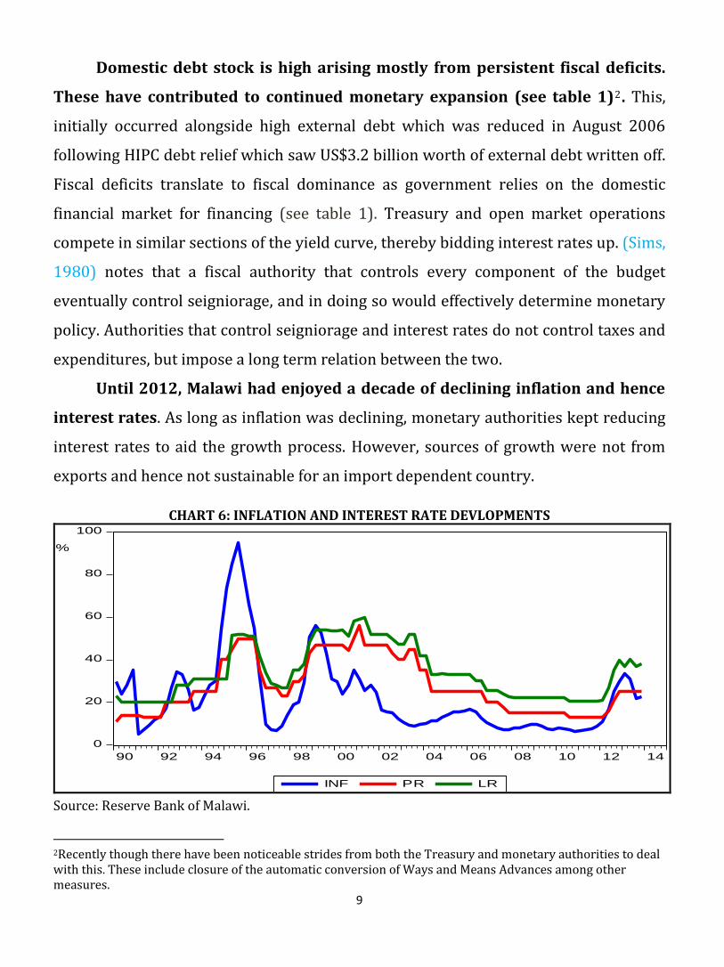
Domestic debt stock is high arising mostly from persistent fiscal deficits.

These have contributed to continued monetary expansion (see table 1)2. This,

initially occurred alongside high external debt which was reduced in August 2006

following HIPC debt relief which saw US$3.2 billion worth of external debt written off.

Fiscal deficits translate to fiscal dominance as government relies on the domestic

financial market for financing (see table 1). Treasury and open market operations

compete in similar sections of the yield curve, thereby bidding interest rates up. (Sims,

1980) notes that a fiscal authority that controls every component of the budget

eventually control seigniorage, and in doing so would effectively determine monetary

policy. Authorities that control seigniorage and interest rates do not control taxes and

expenditures, but impose a long term relation between the two.

Until 2012, Malawi had enjoyed a decade of declining inflation and hence

interest rates. As long as inflation was declining, monetary authorities kept reducing

interest rates to aid the growth process. However, sources of growth were not from

exports and hence not sustainable for an import dependent country.

CHART 6: INFLATION AND INTEREST RATE DEVLOPMENTS

0

20

40

60

80

100

90 92 94 96 98 00 02 04 06 08 10 12 14

INF PR LR

%

Source: Reserve Bank of Malawi.

2Recently though there have been noticeable strides from both the Treasury and monetary authorities to deal with this. These include closure of the automatic conversion of Ways and Means Advances among other measures.

10

The growth was largely driven by peasant agriculture, in particular maize production

(a situation that still persists) which though draining foreign exchange, has no

meaningful feedback on foreign exchange generation. The interest rate levels were

therefore not sustainable and were reversed in May 2012 to deal with the ensuing

macroeconomic imbalances.

2.2 MONETARY POLICY

After independence in 1964, the conduct of monetary policy was through direct

instruments. The RBM was then subordinated to the Treasury. By 1989 there was

evident failure of an activist monetary policy as evidenced by widening domestic and

external imbalances. Financial reforms through Structural Adjustment programmes

therefore commenced. Financial market including interest rates were decontrolled,

foreign exchange market was liberalised and more robust fiscal frameworks (often in

the context of IMF-supported stabilization programmes) were instituted. These opened

up space for indirect monetary policy. The RBM Act was thus repealed in 1989, in a way

giving the RBM legal independence. In the1994, the exchange was floated and the

country started to actively pursue monetary aggregate targeting.

The mandate of the monetary authorities is to influence money supply, credit,

interest rates and the exchange rate in order to promote price stability, economic

growth and a sustainable balance of payments position (Part III (1) (d) of the Reserve

Bank of Malawi Act 1989). (Kwalinga, 2007) observes that implementing such a broad

mandate could be practically challenging. Meeting all objectives requires

multidisciplinary approach. The RBM therefore set price stability as its measurable

objective whose achievement would lead to sustainable BOP and GDP positions.

2.3 POLICY FRAMEWORK AND INSTRUMENTS

A monetary policy framework represents institutional arrangement within which

monetary policy is formulated and implemented. There are four major types of

frameworks; namely, direct targeting of interest rates, credit or prices; monetary

11

aggregates targeting; exchange rate targeting, and inflation targeting. 3 . Theory and

evidence show that the choice of any for particular economy is a function of diverse

factors. (Kasekende, 2010 Unpublished) observes that in Africa, there are 18 countries

pursuing monetary aggregate targeting (MAT), 23 countries pursuing exchange rate

targeting while about 6 are either actively pursuing or seriously considering migrating

to inflation targeting.

The pursuit of MAT with reserve money (RM) as an operational target is based on

Fischer’s quantity theory of money (QTM). The QTM directly links price developments

to changes in monetary aggregates given stability of the money multiplier and velocity.

In classical sense, controlling growth of monetary aggregates should ideally lead to

controlling inflation. QTM is expressed as follows:

tttt YPvM

Where Mt is nominal money supply, tV is velocity of circulation, tP is general price level

and tY is real GDP growth. This equations states that the rate of inflation is

approximately equal to the rate of growth of money in excess of the growth rate of real

output given constancy in velocity.

To operationalise the QTM, first real GDP and inflation projections are made by

government. These are combined with the assumed velocity of circulation, i.e. demand

for money and money multiplier to derive money supply growth which is consistent

with arriving at the projected inflation. Since the central bank cannot directly control

money supply growth, it uses its balance sheet items namely Net Domestic Assets (NDA)

and Net Foreign Assets (NFA) to alter liquidity conditions of the banking system. A

ceiling on NDA as well as a floor on NIR is set consistent with desired growth in reserve

money which is eventually set to influence money supply growth on to an inflation

consistent path. These targets are mostly set within the confines of the country’s

economic programme with the IMF programme.

3 These four types of frameworks are implemented within several variations. For detailed discussion of various policy framework see Mishkin (1998).

12

Other than the Open Market Operations which include foreign exchange

operations, the central bank actively uses the policy rate and the Liquidity Reserve

Requirements as monetary policy instruments. The central bank also accords a lender

of last resort to commercial banks through the Lombard Facility.

SECTION 3.0 LITERATURE REVIEW

3.1 THEORETICAL REVIEW

There are contending theories regarding the impact of monetary policy on

nominal and real variable. Recent major views have been put forward by the real

business cycle (RBC) and new-Keynesians school (NKE).

The RBC by (Kydlland and Prescott., 1982) and (Prescott, 1986) contend that

there is no role for monetary policy as the business cycle are a reflection of rational

decisions by economic agents. Attempt to change this would in fact result in suboptimal

outcomes. Disruptions to the business cycle are real and the economy’s position at any

point in time reflect the equilibrium arising from optimising agents’ adjustments to the

economic disruptions. In effect this mean that there is no role for monetary policy in the

short run and that no attempts should be made by monetary authorities to use

monetary policy because this will throw the economy out of the self-achieved

equilibrium. The basic result from the this classical school is that real economic

magnitudes are self-adjusting so that their equilibrium path is independent of monetary

policy-a phenomenon known as neutrality of money.

Contrary to this view, the new-Keynesians find a significant role of monetary

policy in the short-run arising from Calvo pricing. They argue that nominal rigidities in

price and wage adjustments would result in monetary authorities exploiting dividends

from monetary policy (Mankiw, 1985). In the new-Keynesian analysis monetary policy

affects real variables in short-run.

The modern design of monetary policy is tilting towards the use of NK economics

to exploit the Phillips and IS curves which are designed with nominal rigidities

embedded in them. The trade-off between output and inflation in the short-run implies

13

that disinflation would result in temporary output loss and/or increased

unemployment. In the long-run, however, the vertical Phillips curve based on rational

expectations and continuous market clearing, suggests that monetary policy can only

influence prices and not real variables. Thus, monetary policy should aim exclusively at

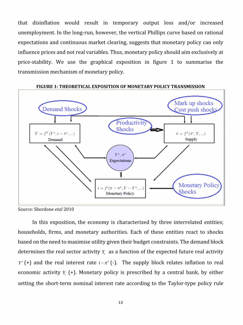
price-stability. We use the graphical exposition in figure 1 to summarise the

transmission mechanism of monetary policy.

FIGURE 1: THEORETICAL EXPOSITION OF MONETARY POLICY TRANSMISSION

Source: Sbordone etal 2010

In this exposition, the economy is characterized by three interrelated entities;

households, firms, and monetary authorities. Each of these entities react to shocks

based on the need to maximise utility given their budget constraints. The demand block

determines the real sector activity tY as a function of the expected future real activity

eY (+) and the real interest rate ei (-). The supply block relates inflation to real

economic activity tY (+). Monetary policy is prescribed by a central bank, by either

setting the short-term nominal interest rate according to the Taylor-type policy rule

14

(Taylor, 1993) or following some money growth rule as in (McCallum, 1988) in

response to developments in inflation and real activity.

The effectiveness of policy innovations depends on the transmission mechanism.

Several theories exist on the transmission process of monetary policy. These include

credit channel, interest rate channel, exchange rate channel, asset price channels and

expectations channel. These channels have mainly been discussed within the variants

of IS-LM-framework proposed by Keynes and formalised by (Tobin, 1969)4.

3.1.1 The interest rate channel

Under the conventional Keynesian interest rate channel, an increase in short-

term interest rates following changes in monetary policy increases the cost of capital,

and hence depresses spending and hence inflation. Evidence of effectiveness of this

channel in Africa has been documented by (Al-Mashat etal, 2007) and (Cheng, 2006) for

Egypt and Kenya, respectively. This channel is not without critics. For example,

(Bernanke and Gertler, 1995) argue that monetary policy has large effects on purchases

of long-lived assets which should be more responsive to real long-term rates than real

short-term rates.

3.1.2 The money supply channel

Contrary to the interest rate view of monetary policy transmission, (Friedman

and Schwartz, 1963) show that the level of prices in the economy reflects money market

conditions arguing for exogeneity of money. Beginning from equilibrium, a reduction in

money balances which can be effected by monetary authorities will reduce aggregate

demand and hence prices and vive-versa. Evidence in support of this channel is

documented for both developed economies, (Friedman and Schwartz, 1963) and less

developed economies, (Chimobi, E and Igwe, O, 2010) for Nigeria; this school too is not

4 Recently, the transmission mechanism has been discussed using the DSGE models which takes account of expectations see for example Gali and Monacelli (2005).

15

without controversy with recent criticism coming from the NKE that money is a veil and

has no impact of real variables, strictly arguing for the potency of interest rates.

3.1.3 The credit channel The credit channel explores financial market imperfections, particularly a wedge

between externally and internally raised investment funds-external financing premium,

(Bernanke and Gertler, 1995). The size of this premium is a reflection of market

imperfections, and a change in market interest rates due to monetary policy is positively

related to a change in the premium, hence credit conditions, money supply, prices and

output. The credit channel is embedded under the balance sheet and the bank lending

channels. In the former, as monetary policy tightens, borrowers’ balance sheets

weakens, lowering their collateral value and raising external finance premium. This

eventually raises adverse selection and moral hazard problems, leading to curtailment

in lending and investment spending. The bank lending channel posits that a disruption

in the supply of bank loans resulting from tight monetary policy makes loan-dependent

producers incur costs associated with finding new lenders. This directly increases their

external finance premium, lowers the levels of borrowing, and reduces real economic

activity.

3.1.4 The exchange rate channel With flexible exchange rates, a rise in domestic real interest rates resulting from

tighter monetary policy stance results in net capital inflows due to interest rate

differentials. This leads to domestic currency appreciation, as well as a fall in exports

and hence output. Additionally, the appreciation makes imports more cheap, a leakage

in the national income identity which lowers aggregate output. Changes in the exchange

rate, therefore, have implications for individual spending, and firms’ investment

behaviour, price stability and employment. Viability of the exchange rate channel is

documented for Ghana by (Ocran, 2007) and for Malawi by (Mangani, 2012).

16

3.1.5 Expectations Channels

Under this channels, changes in policy rates change economic agent’s

expectations of future interest rate path, growth and inflation. These expectations often

affect decisions of firms and households about current saving and investment choices

which then affect price of labour, goods, services and assets.

In summary, the Keynesian advocate that short-term real interest rates changes

are more effective, while monetarists view changes in money supply as more potent.

Meanwhile, the International Monetary Fund (IMF) lends support to the monetarists by

extensively using the financial programming framework for its policy advice to the

majority of the sub-Saharan African countries, including Malawi. Although, it remains a

research issue, literature converges on the fact that long-run effects of monetary policy

fall almost entirely on prices, with no discernible impact on the real variables but

nominal rigidities help to exploit the dividends in the short-run, (Walsh, 2010).

2.2 EMPIRICAL REVIEW

In its regional economic outlook (IMF REO SSA, 2010) the IMF uses single

equation and panel VAR frameworks to study effects of monetary policy on Sub-Sahara

African countries. They find that a shock to reserve money increases output, inflation,

and monetary aggregates, and leads to exchange rate depreciation in floating exchange

rate regimes. This implies that money is a strong determinant of inflation in Sub-

Saharan-African countries contrary to the weak links observed in advanced countries5.

The study also finds strong evidence of price puzzle. An increase in the discount rate

depresses growth, but, somewhat anomalously increases inflation and depreciates the

exchange rate. These findings cast doubt on use of interest rates as an active monetary

policy instrument in Africa. Rather, the evidence renders credence to monetary

aggregate targeting in the region. They however point out that the influence of

monetary policy on growth is weakened by supply shocks and changes in risk premiums

at times of global turbulence, a feature that warrants further analysis.

5 See Castelnouvo (2012)

17

Studies specific on Malawi remain unsynchronised. (Mangani, 2012) uses a VAR

framework and demonstrates that that the Policy rate does not transmit to changes in

inflation. The study further finds evidence that reserve money and broad money had no

discernible impact on prices contradicting (IMF REO SSA, 2010). The exchange rate is

found to have significant impact on prices, a finding which is consistent with small open

economies whose production and consumption systems are import dependent. The

study however did not income real GDP and this may have influenced observed results.

(Simwaka etal, , 2012) uses an error correction model and finds that inflation in

Malawi is driven by demand and supply factors. They find that money supply growth is

positively related to prices with a lag of three to six months. These findings stand in

contrast with (Mangani, 2012) but consensus emerges on the potency of exchange rate.

(Shawa, 2012) finds that money demand is stable, positively responds to changes

in GDP. He also finds significant but low response of money to changes in interest rates.

The stability of the money demand points to the fact that monetary aggregate targeting

remains relevant for Malawi.

(Ngalawa and Viegi, 2011) argues that Monetary Authorities have employed

hybrid operating procedures using the Policy rate as well as Reserve money. The study

also finds that after the 1994 floatation of the Kwacha, the role of the exchange rate

became conspicuous while the role of money and bank lending in the monetary policy

transmission process became enhanced. He notes that monetary policy transmission

evolved to become clearer after the 1994 floatation of the Kwacha. The finding that the

transmission process became enhanced after adoption of the flexible exchange rate is

revealing to monetary authorities especially in light of a recent (May 2012) re-launch

of the floating exchange rate.

(Lungu etal, 2012) find that money demand is insensitive to changes in interest

rates in the short run but weakly significant in the long-run. This insensitivity brings

difficulties in the implementation of the reserve money programming framework.

18

(Mwabutwa etal, 2013) do not find evidence of the existence of the price puzzle

and argue that from 2000, after financial policy reforms, monetary policy transmission

has performed consistently with predictions of economic theory. He finds evidence that

transmission mechanism is not observed prior to reforms; is blurred during the reforms

and gets clearer after reforms.

FIGURE 2: SUMMARY OF RESEARCHED TRANSMISSION CHANNELS ON MALAWI

Source: Authors’ Summary

In summary, further research on effectiveness of monetary policy in Malawi is

necessary based on the following observations: Firstly, some studies e.g. (Shawa, 2012)

use low frequency series in contrast to high frequency analysis required by monetary

authorities. Other studies e.g. (Ngalawa and Viegi, 2011)6 use tobacco as a related series

to interpolate GDP. Significant strides have been made to the extent that other sectors

are now becoming more prominent (see appendix VII). (Simwaka etal, , 2012) use the

index of industrial production to proxy real GDP activity, a subject that still lacks

unanimity for countries with low industrialisation.

Secondly, several fundamentals have changed in Malawi. There has been a shift

from administered pricing to automatic pricing for fuel and automatic adjustment of

electricity and water tariffs (May 2012) . In terms of economic structure, there has been

6 Uses Chen (2006)

19

a modest increase in the share of vending (see appendix VII). The exchange rate is also

not without controversy, having been on stop, reverse and go path. Inability to control

for these changes in the data generation process in most studies and proceeding to the

application of standard econometric techniques reduces the credence of findings.

Finally, most studies have used error correction techniques in the VAR

framework. (Sims, 1992) argues that price puzzles may result from imperfectly

controlling for information used by researchers in their models, a fact that (Soares,

2011) empirically demonstrates.

In view of the diverse findings and the divide in modelling approaches on the

subject, this study contributes to the policy debate by digressing from the conventional

VAR to a Factor Augmented VAR (FAVAR) approach after controlling for potential

breaks and using the Principal Component Analysis. Including factors in the VAR

widens the information set and exposes a coherent picture of the effects of monetary

policy innovations by improving precision of the impulse responses. Since the

pioneering work of (Bernanke and Boivin, 2003) and (Bernanke etal, 2005), several

studies have used the FAVAR; among others; (Zuniga, 2011) on Mexico and Brazil and

(Kabundi and Ngwenya, 2011) on South Africa. The findings from these studies have

disproved price puzzles and have been more informative than those derived from

conventional VAR.

SECTION 4.0 METHODOLOGY

4.1 THE VECTOR AUTOREGRESSIVE FRAMEWORK

Correlation of macroeconomic variables is a fact. Making distinction between

endogenous and exogenous policy shocks therefore becomes difficult, (Stock and

Watson, 1989). To deal with these, the VAR, commonly used for forecasting systems of

interrelated time series and analysing the dynamic impact of random disturbances on

the system of variables becomes handy. The VAR was introduced by (Sims, 1980). This

paper sidesteps structural modelling but harnesses the dynamic impact of random

disturbances by treating every endogenous variable in the system as a function of the

20

lagged values of all of the endogenous variables in the system and an exogenous shock.

The mathematical representation of a VAR is:

ttptpyt xyAyAy ....11 1

Where

ty is a k vector of endogenous variables, and tx is a vector of exogenous

variables, and A and B are matrices of coefficients to be estimated while te is a vector of

innovations that may be contemporaneously correlated but are uncorrelated with their

own lagged values and uncorrelated with all explanatory variables. Since only lagged

values of the endogenous variables appear on the right-hand side of the equations,

simultaneity is not an issue and OLS yields consistent estimates. Moreover, even though

the innovations may be contemporaneously correlated, OLS is efficient and equivalent

to Generalised Least Squares (GLS) since all equations have identical regressors.

Considering the shortcoming of the VAR, precisely inability to control for all the

information, we augment the model with a factor computed from as many series as

available and estimate a Factor Augmented Vector Autoregressive model.

4.2 FACTOR AUGMENTED VAR

The model detailed below and much of its notation follows (Bernanke etal, 2005).

Let tY be an 1MX vector of observable economic variables. Contained in

tY are policy

variables and observable measures of real activity and prices. The conventional

approach of estimating VAR is to use vector tY alone. In practice, however, vast

information is not in this vector and could be extremely relevant to policy dynamics.

Let this unobserved information set be condensed in a second vector, 1KX

denoted as tF . K is expected to be relatively small as the FAVAR is a data reduction

technique. (Bernanke etal, 2005), observes that tF can be construed as reflecting

theoretically motivated concepts such as unobserved economic activity, price

pressures, or credit conditions that cannot easily be represented by one or two series

but rather are reflected in a wide range of economic variables. We model the joint

dynamics of the two vectors tY and

tF as:

21

t

t

t

t

t

Y

FL

Y

F

1

1)( 2

Where L is a lag polynomial of finite order d. The error term t is orthogonal. If the

terms in L which relate tY and

tF are all zeros, the system degenerates to a standard

VAR. If not then equation 2 becomes a factor augmented vector auto regression

(FAVAR). Because the FAVAR model nests standard VAR, estimation of equation 2

allows for easy comparison and provides a way of assessing the marginal contribution

of the additional information contained in tF .

(Bernanke etal, 2005) note that if the true system is a FAVAR, estimating a

standard VAR system in tY excluding

tF will lead to biased estimates. In fact, it may be

the case that the most realistic description of the information structure is that the

central bank and the econometrician truly observe only the policy instrument (the

nominal interest rate), as well as a large set of noisy macroeconomic including GDP,

inflation and other indicators. If the size of the information set is small enough, it can be

directly included in tY . But practically it will be large and the VAR would suffer from

over-parameterisation.

Equation 2 however cannot be estimated directly because the factors are

unobservable. Let tX be the 1NX matrix of the informational set, such that MKN .

We can assume that the information time series tX is related to the factor and the actual

series by the following equation:

tt

y

t

f

t YFX 3

where f is an NXK loading matrix of the factor while y is an NXK loading matrix of

the observable variables. t is an 1NX vector of error terms which are marginally cross

correlated. Equation 3 states that tY and tF characterize common forces that drive the

dynamics of tX . Although tX in equation has contemporaneous relationship with

22

independent variables, the equation can be modified without loss of generality and

meaning by including lags of the factors.

Just like the unrestricted VAR, the FAVAR does not impose prior restriction on the

relation among tX , tF andtY . (Sims, 1980) argues that imposing prior structural

constraints in modelling the behaviour of the economy may result in potential gains but

these gains must be weighed against biases that may result if those restrictions are

wrong (which often is the case). The implication of this is that most structural models

including SVAR and the recent DSGEs if wrongly specified might be ill-suited to study

monetary policy dynamics.

We use the triangular orthogonalization of the variance-covariance matrix to

identify our FAVAR system. This is achieved by estimating the reduced form FAVAR

model, then computing the Cholesky factorization of the covariance matrix of the model

(Lutkepohl, 1993). This ensures that shocks to the VAR system can be identified as

shocks to the endogenous variables in each equation. The approach adopted in the

literature is to place policy variables last in the ordering. The basis for this is the

assumption that policy variables can influence non-policy variables

contemporaneously as well as with a lag, while the non-policy variables themselves can

only be influenced by the policy variables after a time-lag due. To account for the

uncertainty of the "generated regressor" in the second step we implement a bootstrap

procedure, based on (Killian, 1998) when computing impulse response functions.

The factor can be estimated using two procedures. The first is to use the Principal

Component Analysis (PCA) which is not parametric to recover a common space spanned

by the factors in tX to extract the factors. The other approach is to use a single step

Bayesian likelihood approach. (Bernanke and Boivin, 2003) use both procedures and

find similar results and conclude that use of both methods in one analysis is redundant.

We therefore use the two step process because of its superiority in handling data

irregularities as it can take series of different frequencies and its computational

23

simplicity. In the first step, the factors are estimated using the PCA methodology while

the second steps involves incorporating the estimated principal components in the VAR

model to generate the FAVAR model.

4.3 THE PRINCIPAL COMPONENT ANALYSIS (PCA)

The PCA owed to (Hotelling, 1993), is a data reduction methodology that

performs ordinary correlations and extracts common components driving a group of

series. Given NXP matrix of data X of rank order r, 'UDVX where U and V are modelled

as orthonormal matrices of the left and right singular vectors and D as a diagonal matrix

containing the singular values. Vector X can be modelled as 'ABX , where A is an n x r

matrix, and B is a p x r matrix. Both matrices are of rank r. Matrix A are principal

component score and B is a loading matrix. Let be a dispersion matrix of X and

performing Eigen Decomposition

'LL

Where L is the PXP matrix of eigenvectors and is the diagonal matrix with

eigenvalues on the diagonal. These eigenvectors are by construction orthogonal such

that mILLLL

''' . We can write, 1'2/ LnA B and ''2/ LnB B . If we set 1 YLDU , LV

and 2/1)( nD then,

YLDnA B '2/ ,

DLnB B ''2/ ,

Where 10 , is a factor which adjusts relative weighting of L and 'L vectors and

the terms involving are scaling factors where },0{ . Our interest is matrix A which

is interpreted containing the weighted principal components scores which will be used

in our second stage of estimation (FAVAR); and B is the weighted principal components

loadings.

24

However, Principal components A have in them influence from policy variables,

e.g policy rate because they were jointly estimated. It will be improper to use these in

the FAVAR model without extracting the influence of the policy variables. Since the

influence of these policy variables is unknown upfront we follow (Bernanke etal, 2005)

and estimate their coefficients by running a multiple regression of the following

format7:

4

Where SMA is constructed by taking principal components for the slow moving

variables which are not contemporaneously affected by the policy variables; and PV are

our policy variables. The final principal components to be included in the FAVAR is

computed as:

5

The number of principal components can be as many as the information set. Inclusion

in the FAVAR will depend on whether additional components add value to the results.

We now proceed to estimate a VAR in tF and Yt which we denote as FAVAR.

4.4 DATA AND ESTIMATION

In line with our theoretical expose, the observed variables are presented in Table

8. Details of variable definition is provided in appendix I. The model is estimated using

E-views using Quarterly data from 1990 to 2013.

Malawi does not capture quarterly GDP statistics. We therefore follow several

studies that have used univariate filters to interpolate and generate quarterly GDP using

the Constant match average method 8 which assign the same value to all quarterly

observations arising from a particular low frequency data point. In this case the value

7Literature does not place emphasis on diagnostic tests for this equation, see Bernanke etal (2005) 8Alternative Univariate interpolation methods are explained in E-views User Guide I PP 154. Other advanced

interpolation methods are discussed in Chow and Lin (1971) and Harvey and Pierse (1984) who use Kalman filters.

3

1

ˆ

i

it PVAF

t

i

i PVSMAA

3

1

1ˆ

25

of the lower converted series is chosen so that the sum of the high frequency

observations for a particular period matches the low frequency observation is divided

by the number of observations.

Table 2: Model Variables

Category Variable Data Source

Policy Instruments Reserve Money (RM)

Policy Rate (PR)

Exchange Rate (ER)

Reserve Bank of Malawi

Intermediate Variables Lending rate (LR)

Broad Money (M2)

Exchange rate (ER)

Reserve Bank of Malawi

Goal variables Inflation rate (inf)

Real GDP (GDP)

National Statistics Office-

Malawi

Other (1) Information set (X) All variables in the

information set at the

hands of the monetary

authorities

Other (2) Factor (F) Generated by the Principal

Components Analysis

Methodology from

information set (x)

Choosing information to include in Xt is not a haphazard issue. Although (Stock

and Watson, 2002) argue that more data is always good, (Boivin and Ng, 2005)

demonstrate that in practice this may mean using more of the same data since most

series are related. They also investigate this in the context of a forecasting exercise and

find that it is possible to forecast equally well, and perhaps marginally better, by using

factors from fewer screened series. (Bernanke etal, 2005) shows that the pre-screening

of series is largely an ad hoc process.

26

Malawi has undergone several structural changes. Since the VAR model cannot

capture dummy variables directly, we follow (Filmer and Pritchett, 2001) to extract this

information through the principal component analysis. However, to locate dummy

variables, we follow (Bai and Perron, 2003) Multiple Break Point Test.

Tests for structural parameter instability and structural change date back to

(Chow, 1960) who tested for regime change at a priori known dates using an F-statistic.

More recently, (Bai and Perron, 2003) provide theoretical and computational results

that further extend the Quandt-Andrews framework by allowing for multiple unknown

breakpoints and relax the assumption of knowing the break apriori. Following (Bai and

Perron, 2003) we use least squares to regress selected number of data extracted from

our information set on a constant as a dependent variable 9 . The test allows for a

maximum number of breaks, employs a trimming percentage of 15% and uses the 0.05

significance level for the sequential breaks.

The joint results for the suggested breaks are presented in Appendix III. From the

results, three structural breaks are determined namely 1993(Q3), 1997(Q1) and

2009(Q1). Using the “Know thy economy” principle we also include 2012(Q2) as

another potential break to capture significant changes in monetary and exchange rate

policies that took place following change in the political regime. We follow (Filmer and

Pritchett, 2001) and proceed to construct four dummy variables related to these period.

These dummy variables, together with our information set of 15 variables are used to

construct principal components10. While developed countries use a large volume of

information set e.g. (Bernanke etal, 2005), literature does not provide specific guidance

for Low Income Countries in terms of how many variables can be included in the

information set. This issue in LICs is further complicated by challenges of data

9These variables are Narrow money, Nonfood inflation, Food inflation, Treasury bill rate, Lending rates, and Private sector credit, Index of industrial production, Deposit rates and Commercial bank holdings of net foreign assets. 10Greenacre, Michael and Blasius, (2006) use Multiple Correspondence Analysis to extract common components where dummy variables need to be considered.

27

availability. The variables in our information set have been chosen based on their

economic links to the monetary policy instruments11.

A graphical exposition of FAVAR variables in Appendix II suggests that some of

the variables could be trend stationary. Despite this, the models were estimated in

levels using the ordinary least squares (OLS) method. The benefit in estimating the

models in levels arises from the fact that the data would retain the desirable statistical

properties and causal interrelationships that could be lost in the process of differencing.

Indeed, (Bacchetta and Ballabriga, 2000) and (Braun and Shioji., 2004) adopt the same

procedure.

We specify FAVAR using recursive ordering which imposes the identifying

assumption that the unobserved factors do not respond to monetary policy innovations

within the period, in our case quarterly. (Bernanke etal, 2005) argue that we need not

impose that assumption on the idiosyncratic components of the information variables.

We instead define two categories of information variables: “slow-moving” and “fast-

moving.” Slow-moving variables are assumed not to respond contemporaneously to

unanticipated changes in monetary policy e.g. Index of Industrial Production. In

contrast, fast-moving variables are allowed to respond contemporaneously to policy

shocks e.g. Private sector credit. Slow moving variables are therefore placed at the top

while fast moving and policy variables are ordered last in the model.

SECTION 5.0 RESULTS

5.1 VAR Results

In order to infer the value added by the FAVAR to VAR analysis we first present

impulse response results from an ordinary VAR12. All models are estimated at lag 1

chosen based on Schwarz Information Criteria (see appendix V).

11In this case we considered the economic links between the exchange rate, policy rate and money supply to each of the variables. For want of space and as standard practice with other FAVAR studies, we do not present these for all variables as is done with those that have been used to construct our FAVAR in Appendix 1. 12All diagnostics pertaining to the validity of the estimated VAR are presented in appendix iv. The impulse responses are based on Kilian (1998).

28

FIGURE 3: IMPULSE RESPONSE FUNCTIONS FOR ORDINARY VAR

Results from the VAR impulse response functions are consistent with the ones

reported by (IMF REO SSA, 2010) for sub-Saharan African countries which show that

GDP counter intuitively rises as policy rate is raised. Most of the results are also

consistent with (Mangani, 2012).

Two critical results motivate us to take the discussion further using the FAVAR.

First, is the price puzzle finding i.e. that prices respond positively to an interest rate hike

though not statistically significant. Furthermore, that GDP also counterintuitively rises

when the policy rate is hiked. Second, is the liquidity puzzle i.e. the finding that money

supply increases when policy rate is increased. These, it has been argued in literature

29

may result from inability for the econometric models to capture precisely the whole set

of information that the central bank takes into account when setting the policy rate13.

5.2 FACTOR AUGMENTED VAR RESULTS

5.2.1 IMPULSE RESPONSES

Impulse response for the FAVAR take account of only one factor. Although the

number of components generated was equal to the number of variables in the

information set i.e. 18, successive addition of subsequent factors neither improved nor

worsened results. Therefore all the information excluded in the conventional VAR was

deemed to have been captured by the first factor.

Strikingly different from the VAR results, the price puzzle completely disappears

as the response of inflation turns out to be negative following one standard deviation

innovation to policy rate. This finding which is in contrast to (Mangani, 2012) and (IMF

REO SSA, 2010) corroborates (Mwabutwa etal, 2013)14 and (Muhanji etal, 2013) who

use Time Varying Parameter VAR and Dynamic Stochastic General equilibrium

frameworks, respectively, and disprove the existence of price puzzle in Malawi.

(Bernanke etal, 2005) using US data found a similar result. The decline in inflation picks

after 4 quarters and reverts to the steady state after 13 quarters.

GDP negatively responds to an interest rate shock in the short-run, a finding that

is consistent with New Keynesian thinking that with nominal rigidities as described in

(Gali, 2008), monetary policy is indeed able to influence real variable like GDP in the

short-run. This finding contradicts (IMF REO SSA, 2010) on sub-Saharan Africa and is

not revealed using the conventional VAR estimation above. The response of GDP to

inflation returns to steady state and dies off after 13 quarters signifying the applicability

of the classical long run neutrality of Money.

13 See Sims, 1992 14 The author goes further to argue that it is the transmission mechanism that has evolved and that after the adoption of the flexible exchange rate in 1994, transmission mechanism became much more clear, a finding that is corroborated by Ngalawa etal (2011)

30

Furthermore, another pronounced counterintuitive result where money supply

is positively correlated with a rise in policy rate, (IMF REO SSA, 2010), disappears in the

FAVAR simply leaving money supply non responsive to changes in policy rate. The

implication of this finding is that money supply creation could be fiscal driven.

Results further show that there is a trade off in the use of either policy rate or

money supply innovations in terms of stabilising inflation and output. It takes longer

for the two variables to stabilise after a shock to money supply process than it does

when policy is implemented using the interest rate tool. Precisely, inflation and GDP

return to steady state values after 16 and 19 quarters, respectively following a one

standard deviation shock to money supply process. It, however, takes only 13 quarter

for both, inflation and GDP to fall back to the equilibrium path after a one standard

deviation shock to the policy rate.

FIGURE 4: FAVAR IMPULSE RESPONSES

-0.5

0.0

0.5

1.0

2 4 6 8 10 12 14 16 18 20 22 24

Response of F to GDP

-2

0

2

4

6

2 4 6 8 10 12 14 16 18 20 22 24

Response of GDP to INF

-2

0

2

4

6

2 4 6 8 10 12 14 16 18 20 22 24

Response of GDP to M2

-2

0

2

4

6

2 4 6 8 10 12 14 16 18 20 22 24

Response of GDP to PR

-8

-4

0

4

8

2 4 6 8 10 12 14 16 18 20 22 24

Response of INF to F

-8

-4

0

4

8

2 4 6 8 10 12 14 16 18 20 22 24

Response of INF to GDP

-8

-4

0

4

8

2 4 6 8 10 12 14 16 18 20 22 24

Response of INF to M2

-8

-4

0

4

8

2 4 6 8 10 12 14 16 18 20 22 24

Response of INF to PR

-5.0

-2.5

0.0

2.5

5.0

7.5

10.0

2 4 6 8 10 12 14 16 18 20 22 24

Response of M2 to PR

-.2

-.1

.0

.1

.2

2 4 6 8 10 12 14 16 18 20 22 24

Response of LNXR to PR

-4

-2

0

2

4

6

2 4 6 8 10 12 14 16 18 20 22 24

Response of PR to F

-4

-2

0

2

4

6

2 4 6 8 10 12 14 16 18 20 22 24

Response of PR to GDP

-4

-2

0

2

4

6

2 4 6 8 10 12 14 16 18 20 22 24

Response of PR to LNXR

Response to Cholesky One S.D. Innovations ± 2 S.E.

31

We also find significant response of inflation arising from money innovations in

both conventional VAR and FAVAR. When money supply expands, inflation picks up. A

natural policy extension to this is that controlling the growth of money would reduce

inflation. But Money supply does not respond to changes in interest rate. Put differently,

money supply is significant but the credit channel is impotent. This finding alludes to

the role of fiscal dominance in Malawi and is reflected in low correlation of private

sector credit and policy in chart 5.

The study further confirms the finding by (Mangani, 2012) and (Simwaka etal, ,

2012) that a depreciating exchange rate raises inflation and that an increase in real

incomes eventually leads to a decline in inflation.

Another issues relevant for policy is the apparent non-responsiveness of the

exchange rate to changes in the policy rate. Theoretically, a rise in policy rate, through

the uncovered interest parity phenomenon is expected to lead to a surge in foreign

inflows and hence exchange rate appreciation. However portfolio inflows are largely

non-responsive to interest rate changes in Malawi.

The significant response of inflation to the “underlying factor” is reminiscent of a

significantly large volume of information that is left out when other factors are not

included in explaining the inflation dynamics.

In summary, our result completely eliminate the price puzzle and partially

resolves the liquidity puzzle leaving overall money supply non-responsive to changes

in interest rate. The latter could result from cancelling off effects between private sector

credit reduction and expansion in credit to government. Policy rate increases coincide

with heightened fiscal financing requirements. Therefore as private sector credit

contracts15, following a rise in interest rate, the government financing requirements

increase through higher interest rate payments thereby necessitating further recourse

15This finding is confirmed in IMF REO (2010) where private sector credit is included in the model. It is found that private sector credit declines when interest rates are hiked. A part from private sector credit expansion another source of monetary expansion is from fiscal injections which have the potency to overshadow the response of overall Money supply to policy rate changes.

32

to domestic borrowing which eventually expands money supply. This may exert a

netting off effect leaving the overall impact of policy rate innovations on money supply

negligible. In this case, effectiveness of the policy rate as a monetary policy instrument

will be pronounced when fiscal borrowing significantly reduces. The findings also

confirm the authorities’ drive to keep the policy rate tight as long as money supply and

inflation are rising and exchange rate is depreciating.

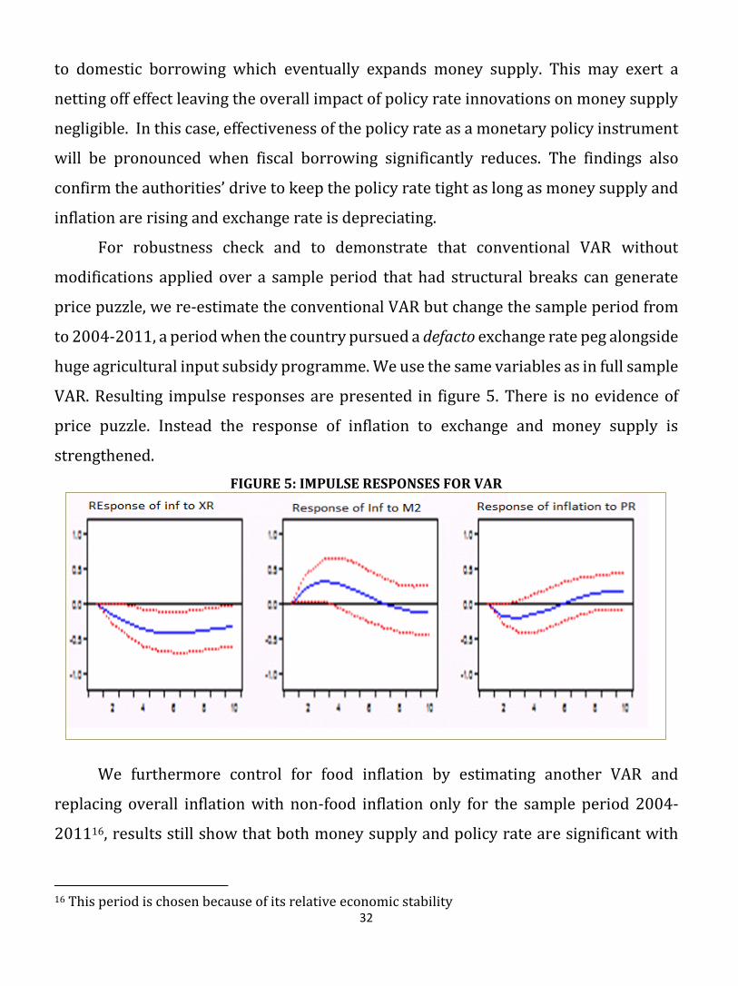
For robustness check and to demonstrate that conventional VAR without

modifications applied over a sample period that had structural breaks can generate

price puzzle, we re-estimate the conventional VAR but change the sample period from

to 2004-2011, a period when the country pursued a defacto exchange rate peg alongside

huge agricultural input subsidy programme. We use the same variables as in full sample

VAR. Resulting impulse responses are presented in figure 5. There is no evidence of

price puzzle. Instead the response of inflation to exchange and money supply is

strengthened.

FIGURE 5: IMPULSE RESPONSES FOR VAR

We furthermore control for food inflation by estimating another VAR and

replacing overall inflation with non-food inflation only for the sample period 2004-

201116, results still show that both money supply and policy rate are significant with

16 This period is chosen because of its relative economic stability

33

respect to inflation and conform to theory. These result are reflected in table 3 where a

negative relationship between money supply and inflation is depicted for the period

2004 to 2011, which if not controlled for in the estimation processes, has tended to

contribute to price puzzle findings. One can therefore observe that the transmission of

monetary policy may not necessarily be divorced from the monetary and exchange rate

policy frameworks within which the policies are implemented.

FIGURE 6: IMPULSE RESPONSES FOR VAR WITH NONFOOD INFLATION

5.2.2 FORECAST ERROR VARIANCE DECOMPOSITION

The variance decomposition reported in Tables 3 and 4 pertain to the FAVAR

structure as the main model. They show the forecast error of inflation at a given horizon

that is attributable to a given shock.

Table 3: Summary of Forecast Error Variance Decomposition

Percentage of Forecast Error Variance attributed to each shock

F GDP INF M2 LNXR PR

En

do

gen

ou

s V

aria

ble

s

F 86.51 10.73 0.34 2.10 0.27 0.07

GDP 4.28 82.21 7.56 3.58 0.06 2.30

INF 61.55 11.21 14.40 8.20 0.86 3.79

M2 38.44 2.12 5.88 53.54 0.00 0.02

EXR 13.47 35.45 3.12 0.98 46.62 0.36

PR 66.75 14.10 1.70 1.82 1.99 13.63

34

A standard result of the VAR literature is that a monetary policy shock explains a

relatively small fraction of the forecast error of real activity measures or inflation. This

finding is reflected in the table 3. For a forecast period of 20 quarters, money supply

and policy rate only explain 3.6 percent and 2.3 percent of the variations in GDP,

respectively. Similarly, only 8.2 percent and 3.8 percent of the variations in inflation are

explained by money and policy rate innovations, respectively. This fact alludes to the

long-run monetary policy neutrality. From Table 4, the factor shows high inertia and

explains about 60 percent of the variation in inflation while inflation explain about 15

percent of its own variation.

Table 4: Variance Decomposition for Inflation

Period F GDP INF M2 LNXR PR

1 61.59 0.06 38.35 0.00 0.00 0.00

2 66.60 3.17 27.48 1.32 0.14 1.30

3 66.75 6.43 20.85 3.21 0.29 2.47

4 65.49 8.93 16.89 5.01 0.42 3.25

5 64.05 10.67 14.50 6.53 0.53 3.73

6 62.80 11.80 13.05 7.71 0.63 4.02

7 61.84 12.49 12.18 8.60 0.71 4.19

8 61.15 12.88 11.66 9.23 0.79 4.29

9 60.69 13.08 11.37 9.66 0.86 4.34

10 60.40 13.16 11.21 9.94 0.92 4.37

11 60.22 13.18 11.13 10.12 0.98 4.38

12 60.11 13.17 11.08 10.22 1.03 4.38

13 60.04 13.15 11.06 10.28 1.08 4.38

14 59.99 13.14 11.05 10.31 1.13 4.38

15 59.96 13.13 11.04 10.32 1.17 4.38

16 59.92 13.13 11.03 10.33 1.21 4.38

17 59.89 13.13 11.03 10.33 1.25 4.38

18 59.85 13.14 11.02 10.32 1.29 4.38

19 59.81 13.15 11.01 10.32 1.33 4.37

20 59.78 13.17 11.01 10.31 1.36 4.37

SECTION 6.0 SUMMARY, CONCLUSION AND POLICY DIRECTIONS

This paper examines the effectiveness of monetary policy in Malawi using a two-

step Factor Augmented Vector Autoregression Model where the first step uses Principal

Component Analysis and second step estimates a FAVAR. Results show that both,

money supply and interest rate innovations have potency to affect inflation. However,

35

interest rate policy is found to be superior to monetary targeting as a stabilisation tool

for both inflation and real GDP.

It is also observed that monetary and exchange rate policy reversals amplify

business cycles and have contributed to divergent results on the subject. Policy

reversals arise from poor institutions. Therefore it is important to improve institutions,

such as central bank independence, goods and money market infrastructure e.g. credit

reference bureaus and legal enforcement of contracts. These will reduce nominal

rigidities and price stickness without necessarily eliminating them thereby enhancing

policy effectiveness.

The significance of exchange rate in the inflation process means that foreign

exchange generation is vital for inflation management. While in the short-term central

bank accumulation of reserves is helpful, in the long-run an increase in exports must

take charge. This will ensure that economic gains are not periodically reversed.

The finding that inflation strongly responds to money supply but money supply

responds weakly to interest rate means that restoring fiscal sustainability and leaving

monetary policy to perform stabilization function rather than financing fiscal deficits

would enhance policy effectiveness.

Meanwhile Monetary Authorities must rely on a vast number of instruments to

implement monetary policy due to data deficiencies17. In this case, precise analysis of

the trade-offs associated with deployment of multiple instrument is vital18.

17This is evidenced by a recent move (September-October 2014) by the central bank where it deployed a mix of policy instruments which included changes in the LRR directives, Policy rate increase, changes in foreign exchange trading rules, rebalancing of the domestic and foreign debt portfolios among others to avert the depreciation of the kwacha. These unconventional monetary tools may also complicate the analysis of the effectiveness of the major policy tools 18Technical capacitation is one of the key interventions in process.

36

SECTION 7.0 REFERENCE

REFERENCES

Al-Mashat etal. (2007). The Monetary Policy Transmission Mechansim in Egypt. IMF Working

Paper WP/07/287.

Bacchetta and Ballabriga. (2000). The impact of monetary policy and banks' balance sheets:

some international evidence. Applied Financial Economics, 15-26.

Bai and Perron. (2003). Computation and Analysis of Multiple Structural Change Models.

Journal of Applied Economterics Volume 18, 1-22.

Bernanke and Boivin. (2003). Monetary Policy in a Data-Rich Environment. Journal of

Monetary Economics, 525–546.

Bernanke and Gertler, M. (1995). Inside the Black Box: The Credit Channel of Monetary

Transmission. Journal of Economic Perspectives, 9(4), 27-48.

Bernanke etal. (2005). Measuring the Effects of Monetary Policy: A Factor Augmented Vector

Autoregressive (FAVAR) Approach. Quarterly Journal of Economics.

Boivin and Ng. (2005). Understanding and Comparing Factor-Based Forecasts. NBER

WOrking Paper No. 11285.

Braun and Shioji. (2004). Technology Shocks and Work Hours: Evidence from Japan. Keizai

Kenkyu, 55(4), 289-298.

Cheng, K. (2006). A VAR Analysis of Kenyas Monetary Policy Transmission Mechanism: How

Do the Central Bank's REPO affect the economy? IMF Working paper WP/06/300.

Chimobi, E and Igwe, O. (2010). Budget Deficits, Money Supply and Inflation in Nigeria.

European Journal of Economics, Finance (19), 52-60.

Chow, G. C. (1960). Tests of Equality Between Sets of Coefficients in Two Linear Regressions.

Economterica, 591-605.

Filmer and Pritchett. (2001). Estimating Wealth Effects Without Expenditure Data-Or Tears:

An Application To Educational Enrollmnets in States of India. Demography, 115-132.

Friedman and Schwartz. (1963). A monetary history of the United States, 1867–1960.

Princeton University Press, Princeton, NJ.

Gali, J. (2008). Monetary Policy, Inflation: An Introduction to the New Keynesian Framework.

Oxford: Princeton University Press.

Hotelling, H. (1993). Journal of Education Psychology (24), 417-441, 498-520.

37

IMF REO SSA. (2010). Regional Economic Outlook for Sub-SAhara African Countries.

Kabundi and Ngwenya. (2011). Assessing Monetary Policy in South Africa in a Data Rich

Environment. South African Journal of Economics Volume 79, Issue 1, 91-107.

Kasekende, L. (2010 Unpublished). Rethinking Monetary Policy for the 21st Century. Kampala

Uganda: Bank of Uganda Working papers.

Killian, L. (1998). Small Sample Confidence Intervals for Impulse Response Functions. The

Review of Economics and Statistics, 218-230.

Kwalinga, S. (2007). The Monetary Policy Reaction Function for Malawi. Zomba, Malawi:

Master of Art Thesis.

Kydlland and Prescott. (1982). Time to Build and Aggregate Fluctuations. Econometrica 50

no.6, 1345-1370.

Lungu etal. (2012). Money Demand Function for Malawi: Implications for Monetary Policy

Conduct. Banks na Bank Systems Issue 1.

Lutkepohl, H. (1993). Introduction to Multiple Time Series Analysis. Springer 2nd ed.

Mangani, R. (2012). The Effects of Monetary Policy on Prices in Malawi. African Economic

Research Consortium publications.

Mangani, R. (2014). Effectiveness of Monetary Policy in Malawi, Evidence from an

Autoregressive Distributed Lag model.

Mankiw, G. (1985). Small Menu Costs and Large Business Cycles:A Macroeconomic Model of

Monopoly. Quarterly Journal of Economy, 529-539.

McCallum, B. (1988). Robustness Propoerties of a Rule for Monetary Policy. Carnegie

Rochester Conference Series on Public Policy, (pp. 173-203). 29North-Holland,

Amsterdam.

Muhanji etal. (2013). Price and Liquidity Puzzles of a monetary Shock: Evidence from

Indebted African Economies. Economic Modelling 33, 620-630.

Mwabutwa etal. (2013). Evolution of the Monetary Policy Transmission Mechanism in Malawi:

A TVP-VAR Approach. University of Pretoria, Department of Economics working

papers.

Ngalawa and Viegi. (2011). Dynamic effects of monetary policy shocks in Malawi. South

African Journal of Economics 79(3), 224-250.

38

Ocran, M. (2007). A Modelling of Ghana's Inflation Experience; !960-2003. African Economic

Research Consortium, Nairobi.

Poole, W. (1970). Optimal Choice of Monetary Policy Instruments in a Simple Stochastic

Macro Model, . Quarterly Journal of Economics 84: , 197-276.

Prescott, E. C. (1986). Theory Ahead of Business Cycle Measurement. Quarterly Review 10, 9-

22.

Shawa, K. c. (2012). A macro-economic diagnosis of the Keynesian Propositions of the Money

Demand Function in Malawi: An error-correction approach. International Journal of

development and Sustainability Vol 1 (1), 31-46.

Sims, C. (1980). Mcroeconomics and Reality. Econometrica, 1-48.

Sims, C. (1992). Interpreting the macroeconomic time series facts: The Effects of Monetary

Policy. European Economic Review 36, 975-1011.

Simwaka etal, . (2012). Money Aupply and Inflation in Malawi: An Econometric investigation.

Intrenational Journal of Applied Economic and Finance, 6(3), 74-88.

Soares, R. ( 2011). Assessing Monetary Policy in the Euro Area: A factor-Augmented VAR

Approach. Working Papers 11/2011.

Stock and Watson. (1989). Interpreting the evidence on money-income causality. Journal of

Econometrics 40, 161-182.

Stock and Watson. (2002). Forecasting Using Principal Components From a Large Number of

Predictors. Journal of The American Statistics Association, 1167-1179.

Taylor, J. B. (1993). Disctretion Versus Policy Rules in Practice. Carnegie-Rochester

Conference Series on Public Policy Volume 39, (pp. 196-214).

Tobin, J. (1969). A general Equilibrium Approach to Monetary Theory. Journal of Money,

Credit and Banking, 1, 15-29.

Walsh, C. E. (2010). Monetary Theory and Policy. Cambridge: The MIT Press.

Zuniga, M. (2011). International Monetary Transmission, a Factor-Augmented Vector

Autoregressive Approach: The Cases of Mexico and Brazil. Business and Economcs

Journal BEJ-26.

39

SECTION 8: APPENDICES

APPENDIX I: VARIABLE DEFINITION

Variable Description

Policy

Rate (PR)

This a monetary policy instrument set by the Reserve Bank of Malawi. It is an

indicator of monetary policy stance and is set based on developments in

inflation, money market rate and prospects for real GDP growth.

Inflation

(Inf)

Is the rate of change in overall level of domestic prices. It is made up of 50.8%

food inflation and 49.2% non-food inflation

Exchange

Rate (ER)

It is the official nominal Malawi kwacha per USD

Reserve

Money

(RM)

It calculated as the sum of currency in circulation, Vault cash and Commercial

bank deposits with the Reserve bank of Malawi

Broad

Money

(M2)

It is the sum of currency outside banks, demand deposits, time and savings

deposits

Read GDP This is the real growth rate of the economy

Lending

Rate (LR)

Average of maximum and minimum commercial banks’ lending rates

Factor Xt Constructed through PCA analysis from the following variables: Index of

industrial production (IIP)*, Food Inflation (FINF), Nonfood Inflation (XINF), 91

day Treasury bill rate (TBR), Deposit Rate (DR), Liquidity Reserve

Requirement(LRR), Fiscal Deficit,(Fisc), Narrow money (M1), Private sector

credit (PSC), Net Credit to Government (NCG), Net Domestic Credit (NDC),

Commercial Banks’ Net Foreign Assets (CBNFA), Crude Oil Price (OILP)*,

Commodity Price Index (COMPI)* and Agriculture Commodity Price Index

(AGCOMPI)*; Dum1(1997Q1), Dum2(1993Q3), Dum3(2009Q3) and Dum4

(2012Q2).

*Denotes Slow-moving variables, otherwise fast-moving

40

APPENDIX II: GRAPHICAL PRESENTATION OF THE MODEL VARIABLES

-15

-10

-5

0

5

10

15

20

90 92 94 96 98 00 02 04 06 08 10 12 14

GDP

0

20

40

60

80

100

90 92 94 96 98 00 02 04 06 08 10 12 14

INF

0

20

40

60

80

100

90 92 94 96 98 00 02 04 06 08 10 12 14

M2

10

20

30

40

50

60

90 92 94 96 98 00 02 04 06 08 10 12 14

PR

-40

0

40

80

120

160

90 92 94 96 98 00 02 04 06 08 10 12 14

RM

0

100

200

300

400

90 92 94 96 98 00 02 04 06 08 10 12 14

XR

APPENDIX III: BAI PERRON MULTIPLE BREAK POINT TEST

Suggested Causes of Breaks There was a big drought in 1992. In 1993, Malawi was undergoing political reforms from single party

to plural political and the referendum was held in this year and this could be responsible for the

structural break. In 2009, the country started experienced economic hardship following imprudent

economic policies which included maintenance of an overvalued exchange rate.

41

APPENDIX IV: VAR DIAGNOSTICS

42

APPENDIX V: FACTOR AUGMENTED VAR DIAGNOSTICS

FAVAR Lag Order Selection Criteria

Sample: 1990Q1 2014Q4 Included observations: 88

Lag LogL LR FPE AIC SC HQ 0 -1518.918 NA 45352087 34.65722 34.82613 34.72527

1 -1006.271 943.7363 897.0385 23.82434 25.0061* 24.30069 2 -957.7100 82.77438 681.7536 23.53886 25.73468 24.42350 3 -911.3279 72.73560 553.9468 23.30291 26.51218 24.59584 4 -853.2446 83.16474 354.3121 22.80101 27.02375 24.50225 5 -787.2042 85.55230 196.4043 22.11828 27.35447 24.22781 6 -731.1803 64.93681 143.9405 21.66319 27.91283 24.18101* 7 -685.3774 46.84389 142.6943 21.44039 28.70350 24.36652 8 -624.3740 54.07118* 110.1200* 20.87214* 29.14869 24.20655

43

APPENDIX VI: EVOLUTION OF EXCHANGER RATE POLICIES

APPENDIX VII: GDP BY ECONOMIC ACTIVITY

Source: National Statistics Office *Mean Preliminary