1

DETERMINANTS OF SCHOOL ATTAINMENT IN TURKEY

AND THE IMPACT OF THE EXTENSION OF THE

COMPULSORY EDUCATION

Idil Göksel

Abstract

The aim of this paper is first to explain the main factors that affect the demand for education in Turkey for boys and girls, then to investigate if there are any differences between genders or not, and finally to try to evaluate the impact of the extension of the compulsory education in Turkey in 1997. It might be concluded that income growth, increase in parents’ education and fertility control contribute positively to children’s school attainment, and their positive effect will be higher for girls than boys. Furthermore the results show that extension of compulsory education increased the total working hours in the households, but it did not have any effect on the probability that the mother starts working or father gets an additional job. On the other hand it had a positive effect on child labor by decreasing the probability of child labor in the households. Another factor that is proved by this study is the fact that due to high drop out rates, increase in school enrollment does not necessarily mean increase in school graduation rates.

I- Introduction

The importance of education in economic development is a known fact. There are

many studies that present the contribution of education to economic growth,

individual and social development. Being a developing country, improvement in

education plays an important role in Turkey’s development, and unfortunately Turkey

does not perform well in terms of education. As Wigley and Wigley (2005) state the

education of Turkey’s adult population is out-performed by most of the countries with

a lower GDP per capita and, with the exception of Brazil, by those countries with a

similar or higher level of per capita income in terms of being literate. In terms of

youth illiteracy only Jamaica, the Philippines and Brazil perform worse than Turkey.

Wigley and Wigley highlight that female illiteracy rate is higher in Turkey than many

other countries. Considering all these, it is important to understand the main factors

that affect the school enrollment in Turkey, and design policies accordingly.

2

On the contrary to the developed countries, Turkey extended its compulsory education

recently. It is important to investigate its effects and see whether this policy is

efficient or not in increasing school enrollment and graduation rates currently. In the

last 15 years, Turkey has showed substantial improvement in literacy for both

genders. The literacy rate of men, which was 89.8% in 1990, became 96% in 2006,

while the literacy rate of women increased from 67.4% to 80.3%1. On the other hand,

there has not been a huge change in the net enrollment rate of primary education

during these years (for boys 95.06% and 92.29%, for girls 88.7% and 87.16%, for the

years 1990 and 2006 respectively), while in high school attainment the net enrollment

rate of men increased from 31.82% to 61.13% in 2006, and of women from 20.59% to

51.95%.

In 1997, Turkey extended length of compulsory primary education from 5 to 8 years.

Before 1997, after 5 years of compulsory education there were 3 years of secondary

school and 3 years of high school after which the students could attend university

depending on their wish and more importantly on their success in university entrance

exam. In 1997, by the rule, the primary education and secondary education were

combined and became compulsory. Although the extension of compulsory education

increased the enrollment of children to the previous middle school (3 years of

education after 5 years of compulsory primary education before the extension); an

increase in enrollment does not necessarily mean an increase in graduation rates.

When the basic education net enrollment rate of 7-15 years old children in 1994 is

compared with the graduation from compulsory education rates of 13-21 years old

children in 2002, 8.59% drop out rate for girls is observed, while in general all the

boys that were enrolled were graduated. It can be concluded that especially for girls

increasing enrollment rate does not necessarily mean a success in improving the girls’

education. Factors that have an impact on girls’ school attainment should be

investigated and improved.

The aim of this paper is first to explain the main factors that affect the demand for

education in Turkey for boys and girls, then to investigate if there are any differences

1 Turkish Statistical Institute Population and Growth Indicators http://nkg.tuik.gov.tr/

3

between genders or not, and finally to try to evaluate the impact of the extension of

the compulsory education in Turkey in 1997.

The outline of this paper is as follows. In the following section there is a brief

literature review. In section III the data is described. It is followed by the section in

which the model and the methodology will be explained. The presentation of

estimation results will take place in section V. Section VI is devoted to analyze the

impact of mothers on school attainment and section VII analyzes the effects of the

extension of compulsory education, and section VIII concludes.

II- Literature Review

There are many papers about the effects of extension of compulsory education on

various things like age of giving child birth, wages, adult mortality, etc. Black at al

(2004) investigate whether increasing compulsory education attainment through

mandatory schooling legislation encourages women to delay childbearing in US and

Sweden, and they find out that extension of compulsory education reduces the teenage

childbearing in both of the countries. As the extension in Turkey took place very

recently it is early to be able to see its effect on childbearing, but we might assume

that if it had positive effect on school attainment in general, then it would also cause a

decrease in the amount of teenage child bearing. In the paper of Lleras-Muney (2004)

causal impact of education on health is examined by following synthetic cohorts using

successive US censuses and using compulsory educations laws from 1915 and 1939

as instruments for education to estimate the impact of educational attainment on

mortality rates. According to the results education has a causal impact on mortality.

Oreopoulos (2006) investigates the income effects of compulsory schooling in Canada

and finds out that mandating education substantially increases adult income and

substantially decreases the likelihood of being below the low-income cut-off

unemployed, and in manual occupation.

In the context of Turkey, by using the data for 1994 and 1999 Dayioglu (2005) makes

a simulation to see the effects of this extension on child labor. In another paper by

Dulger (2004), rationale and objectives of the program are described. Tansel (2002),

4

which is closely related to this paper, explains the main determinants of school

attainment in Turkey for boys and girls separately by using 1994 data. From her paper

it can be concluded that even when the compulsory education was five years there had

not been full enrollment of children to primary school. Here another question arises:

What are the determinants of school attainment in Turkey?

There is a huge literature on the determinants of school attainment especially written

about developing countries. The main determinants that are taken into account are

usually gender, parents’ education, household income, number and gender of siblings,

rural/urban residence, employment of parents, etc. Connelly and Zheng (2003) define

school enrollment as a function of demand, supply and government policy. The

individual decisions about the enrollment made by students or their parents comparing

the costs and benefits of staying at school are considered as demand, while

availability and quality of education forms the supply. In this paper the demand side

of school enrollment and the impact of the specific change in the government policy

(extension of the compulsory education) will be analyzed.

In the previous studies most of the above mentioned factors were found significant

determinants of school attainment, while their degree of impact is different for each

country. In their analysis of 1995 CHIP data, Knight and Song (2000) find that boys

have a higher probability of enrollment and the children, mothers of whom are more

educated than their fathers, have higher school attainment in China. In a more recent

study, again about China, Connelly and Zheng (2002) find that location of residence

and gender are highly correlated with enrollment and graduation, and rural girls are

especially disadvantaged in terms of both enrollment and graduation rates. Other

determinants that are found to be significant in their study are parental education, the

presence of siblings, country level income and village level school rates. Ilon and

Moock (1991) classify the predictors of educational participation under six categories

in their study about Peru: Individual child characteristics, opportunity costs,

socioeconomic factors, school quality, school access and direct school costs. They

find that the monetary costs of schools influence parents’ decisions regarding school

attendance and continuation, and mother’s education is important on children’s

education, especially in low-income households.

5

Holmes (1999) analyzes the demand for schooling in Pakistan and focuses on two

potential sources of bias in the estimation of demand for schooling. She defines the

first source of bias as not distinguishing between currently enrolled children and those

who completed their schooling, which she calls censoring bias. According to Holmes

(1999), second source of bias is the sample selection bias, which she defines as

excluding children who have left the household from the sample in case the decisions

to leave home and to attend school are related. In this study the sample is chosen in

such a way to minimize these biases. Holmes (1999) explains two limitations of the

data in the previous studies about determinants of school attainment. The first is the

fact that surveys measure schooling by the years of education attained, meaning that

the education level is observed in discrete year intervals although the desired level of

schooling is continuous. Her second reasoning as limitation is the existence of a large

mass point at zero years of schooling and similar probability spikes at primary and

secondary completion levels where continuation to the next level is delayed by fees or

entrance examinations. She does not find Ordinary Least Square estimation

appropriate due to non-negativity restriction, the discreteness and the probability

spikes of schooling variable, and advises to use censored ordered probit model which

was proposed by King and Lillard (1983;1987). In this study ordered probit model

will be used, and censoring bias will be controlled.

There might be many factors that have impact on school attainment within a country.

It is important to determine them in order to be able to apply efficient policies to

increase the demand for schooling. Furthermore, discovering the effects of an already

applied policy would be good guide to form the future policies.

III- Data

In this survey two data sets are combined: 1994 and 2002 Household Income and

Consumption Survey of State Institute of Statistics of Turkey. The 1994 survey was

administered to 26,256 households in Turkey, while the 2002 survey was completed

by 9555 households around the country. In the 1994 data, there are 11659 children

between the ages of 16-20 in relation to the household head, while the 2002 data has

3659 children within the same age range in relation to the household head.

6

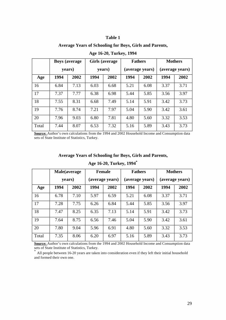
The average years of schooling for children and their parents are given in Table 1 for

the years 1994 and 2002. In general it seems like gender gap between boys and girls

increases with age. By the age 20 the gender gap between boys’ and girls’ years of

schooling becomes more than a year. There is approximately two years of difference

between mothers and fathers average years of schooling. When the average schooling

years compared between 1994 and 2002, an improvement is observed for all

individuals. On average the increase in girls’ years of schooling is higher than the one

for boys, meaning approximately 16% of the gender gap in 1994 was closed in 20022.

Another difference between the two data sets is the fact that 2002 data set does not

have regional variables, so in this paper it will not be possible to investigate the

regional differences.

IV- Model and Methodology

The model used in the first part of this paper and the empirical specification are taken

from Tansel (2002) in which the determinants of school attainment in Turkey are

analyzed for the year 1994. This paper was chosen because she uses the ordered

probit estimate, which is the most appropriate estimate for this work and the reason

will be explained in the following sections. In this survey both 1994 and 2002 data

will be used. As a result it might be also possible to see the effects of extension of

compulsory education on the determinants that have impact on the probabilities of

school attainment, being aware of the fact that the change will not be only due to the

extension of compulsory education. Different from Tansel (2002) the effects of the

number of children in the family and the composition of gender among the children

will be checked. Also the effect of having a grandparent within the family is

controlled, but as it did not have any significant effect in any of the cases it is dropped

out and the results are not presented here. 2 An interesting thing in the table is the fact that although for each age group education level increases monotonically with the age, for 20 years old girls it is lower than the 19 years old ones. This result does not change even when the average year of schooling is calculated for all the people in that age even if they left their family and formed their own household. More interestingly for the ages 21 and 22 it continues to increase monotonically. It cannot be a cohort effect as it happens in both years, so most probably it is a noise in the data.

7

In human capital theory, education is seen as not only a consumption activity but also

an investment to maximize lifetime wealth (Schultz, 1963, 1974; Becker, 1975). Each

individual faces the problem of comparing benefits and costs of additional schooling.

On the one hand additional schooling brings higher future earnings as a benefit, on the

other hand it postpones the entry time of individuals to the labor force. The

individuals will continue to invest in education as long as the marginal rate of return

of additional schooling stays above the corresponding cost of borrowing. As a result

there is a positive relationship between optimal level of schooling and returns to

human capital, while there is a negative relationship between optimal level of

schooling and the cost of schooling.

Tansel (2002) explains that the demand for the schooling of children could be written

as a function of the wages of household members, market prices of inputs, unearned

household income and a set of child and household characteristics. Furthermore if

parents have different preferences for their son’s and daughter’s level of schooling,

this will cause gender specific demand functions for schooling. Tansel (2005) finds

out that women in Turkey may be facing discrimination in the private sector and also

the private returns to schooling are higher in private sector than in public sector. So it

might be suggested that the returns to schooling for women might be lower in Turkey

as they face discrimination in the private sector in which returns to education is

higher. This fact may affect the parents’ decisions about investment level to their

daughters’ and sons’ education, as investing in sons’ education seems to be more

efficient. Besides, parents may predict the expected benefit of educating their son

higher than their daughters’ as daughters join their husband’s household by marriage,

while sons are more likely to provide help for parents in old age. Furthermore

education has some non market benefits to economic development which are difficult

to quantify such as increase in nutrition and health, higher education of children,

lower child mortality and fertility. In literature it is shown that in developing countries

females gain more than males in terms of non market benefits. (King and Hill, 1993;

Schultz, 1995b).

Recent literature documents the important role of parents’ education on children’s

schooling attainment. Parents’ taste for schooling and the genetic factors can be

8

understood from the level of parents’ education level. Besides, mother’s education

may represent home investments, permanent income, opportunity cost of mother’s

time in labor market and efficient household production. As Tansel (2002) states if

schooling is a normal good, the higher income and wealth will lead to higher

schooling attainment, ceteris paribus. Furthermore if schooling is a luxury good,

especially for low income households, then the income effect would be very large.

Schooling has both direct and indirect costs. The budget separated to books, uniforms,

transportation and tuition can be counted as direct costs. On the other hand indirect

costs of schooling, which is the opportunity cost of children’s time that instead they

could spend for household production or labor market participation, also plays an

important role especially in rural areas.

In this paper ordered probit models are formed for middle and high school

attainments. In 1997 the primary and secondary education in Turkey is combined by

extending the compulsory education from 5 years to 8 years. In order to be able to

compare the years of 1994 and 2002 only compulsory and high school attainments are

taken into account. For the year 1994, middle school attainment means 5 years of

compulsory education and 3 years of secondary school, while in 2002 compulsory

education is 8 years. Following Tansel (2002), the latent demand for the desired level

of schooling, S* is defined as:

S* = ^β X + e (1)

where X is a vector of individual and household explanatory variables and e is the

normally, independently distributed disturbance term. ß is the vector of coefficients of

the factors that affects the school attainment. In practice, desired schooling is not

observed, while different levels of education of boys and girls, S is the observed

counterpart of S*. In this case it is better not to use Ordinary Least Squares (OLS) as S

is discrete and OLS assumes that the dependent variable is continuous and unlimited.

Moreover, as level of education takes only positive values, OLS estimation is

inappropriate due to the non-negativity restriction.

Depending on the years of schooling K categories are formed and each individual is

assigned one of these categories. Illiterate individuals have zero year of schooling,

9

while two years of schooling indicates that the individual is literate but not a graduate

of any school. Primary school graduates have five years of schooling and this was the

compulsory amount in 1994. Middle school graduates have eight years of schooling

and this is the new compulsory education amount in Turkey. Finally high school and

university graduates have eleven and fifteen years of schooling, respectively. Those

who have graduate leve l degrees assumed to have seventeen or more years of

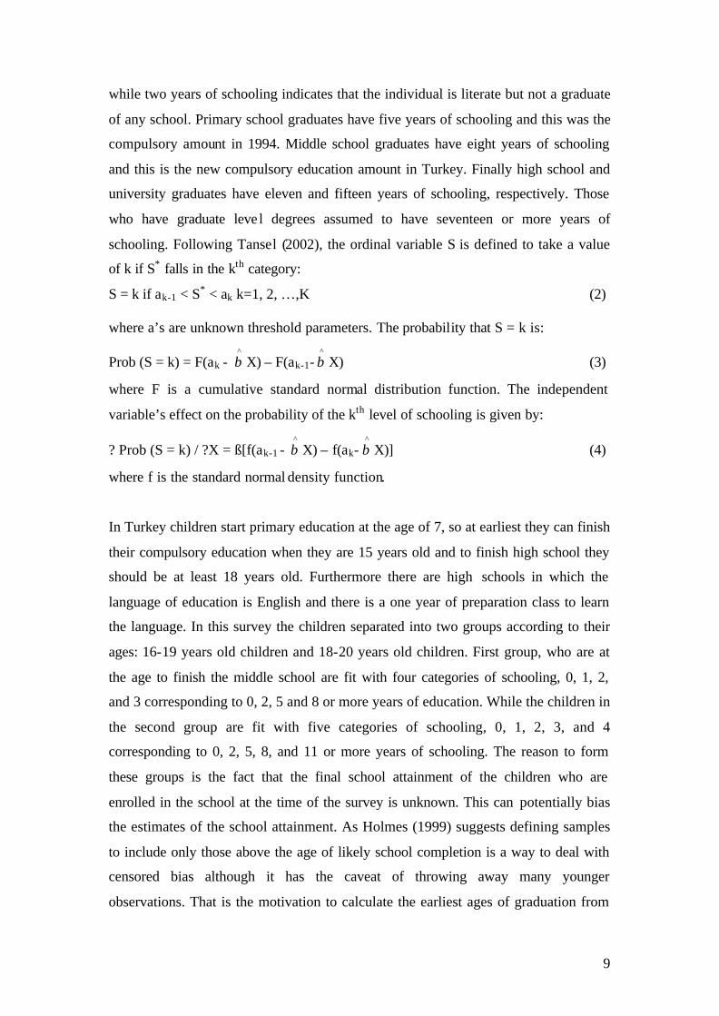
schooling. Following Tansel (2002), the ordinal variable S is defined to take a value

of k if S* falls in the kth category:

S = k if ak-1 < S* < ak k=1, 2, …,K (2)

where a’s are unknown threshold parameters. The probability that S = k is:

Prob (S = k) = F(ak - ^β X) – F(ak-1-

^β X) (3)

where F is a cumulative standard normal distribution function. The independent

variable’s effect on the probability of the kth level of schooling is given by:

? Prob (S = k) / ?X = ß[f(ak-1 - ^β X) – f(ak-

^β X)] (4)

where f is the standard normal density function.

In Turkey children start primary education at the age of 7, so at earliest they can finish

their compulsory education when they are 15 years old and to finish high school they

should be at least 18 years old. Furthermore there are high schools in which the

language of education is English and there is a one year of preparation class to learn

the language. In this survey the children separated into two groups according to their

ages: 16-19 years old children and 18-20 years old children. First group, who are at

the age to finish the middle school are fit with four categories of schooling, 0, 1, 2,

and 3 corresponding to 0, 2, 5 and 8 or more years of education. While the children in

the second group are fit with five categories of schooling, 0, 1, 2, 3, and 4

corresponding to 0, 2, 5, 8, and 11 or more years of schooling. The reason to form

these groups is the fact that the final school attainment of the children who are

enrolled in the school at the time of the survey is unknown. This can potentially bias

the estimates of the school attainment. As Holmes (1999) suggests defining samples

to include only those above the age of likely school completion is a way to deal with

censored bias although it has the caveat of throwing away many younger

observations. That is the motivation to calculate the earliest ages of graduation from

10

the schools and to form the groups accordingly. Furthermore in this survey only

children in relation to the household are taken into account. Finally following Tansel

(2002) the upper bound of age is restricted with 20 as children usually leave the

household of their parents after this age and if the ones above this age are taken into

account it would be an unrepresentative sample. In order to find this out Tansel

(2002) computes the proportion of the own children in the household by age and she

finds that this ratio drops substantially after age 19 for 1994 data. Unfortunately in

2002 survey the question of total number of children is omitted so it is not possible to

investigate the children who left the house. As a result in this paper the same

procedure cannot be repeated for 2002, but three years of extension of compulsory

schooling would not cause children to leave house even earlier than before. If it would

have any affect it would increase the age of house leaving, so it is assumed that the

trend in age of leaving the house would not change drastically in eight years.

Children are separated as boys and girls and following variables are used as

determinants of schooling: Children’s age, squared term of children’s age, education

of parents, two dummies showing whether mother and father are self employed, two

dummies whether only mother or only father is present at the household, logarithm of

total household expenditure, a dummy variable that shows whether the household is

located in the urban area, number of children and percentage of boys or girls in the

household.

Children’s age and squared term in age would show the age effects and whether there

is nonlinear effect of age on schooling. Parents’ education separated into two such as

mother’s and father’s education and the years of schooling they achieved are taken

into account. Parents’ education accounts for both genetic ability of children and the

complementary home learning. Furthermore, parents’ education may also serve as a

proxy for parents’ earnings that could be invested in schooling. Moreover, more

educated mothers may have higher bargaining power in the household and may decide

to invest more on their children’s human capital. Dummies for self employment of

parents are used to investigate whether self employed parents force their children to

work at their own place, or not. In order to understand whether living only with

mother or father affects the school attainment, the dummies for only mother and only

father are used. Total household expenditure is used to proxy for household

11

permanent income as there may be transitory fluctuations in income while savings

allow the smoothing of expenditures over time. The dummy urban is used to observe

whether being in a rural area decreases the school attainment due the fact that in rural

areas there exist fewer schools, less qualified teachers, higher opportunity cost for

children because of farm employment opportunities or child labor needs at home.

Furthermore in rural areas families are more likely to be credit constraint than the

ones in urban areas as rural families operate with less cash per level of consumption.

Another caveat of rural areas is the fact that historically they have lagged behind

urban areas in access to schooling, so the parents of children in rural areas are likely

to have less education than parents in urban areas (Ilon and Moock; 1991). Number of

children is used to capture whether the households are credit constrained, and also to

understand the relationship between fertility and the investment on education. Finally

for the girls’ school attainment determinant, percent of boys in the family is used to

see if there is any gender difference in parents’ mind when they are deciding how

much to invest on their children’s human capital. Likewise percent of girls is used

when estimating boys’ school demand function.

V- Estimation Results for School Attainment

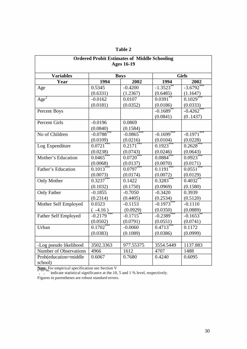
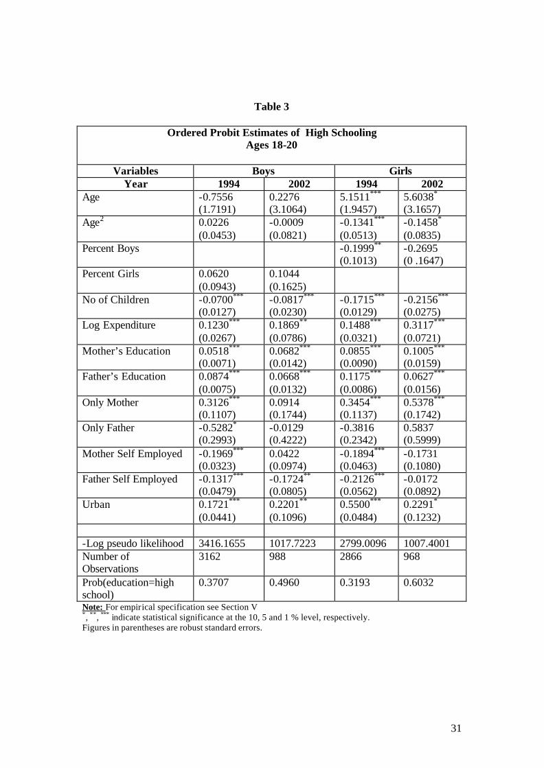
Tables 2 and 3 present the ordered probit estimation results for middle and high

school attainment, respectively. As discussed before for middle schooling, boys and

girls between the ages 16-19, and for high schooling children between 18-20 years are

considered. The following ordered probit estimations are used:

EduBoyi = ß0 + ß1Xi+ ei, and (5)

EduGirli = ß0 + ß1Xi + ei (6)

where EduBoyi and EduGirli are the education levels of boys and girls, respectively,

and Xi is the vector of control variables like the age of the child, the squared term of

the age, the percentage of number of girls in the total number of children in the

household for the first regression and the percentage of number of boys for the second

one, the number of children in the household, the total expenditure of the household,

the number of years that the mother and the father spent for education, dummy

12

variables that take the value one when the child lives with only her mother or with

only her father as a parent, the dummy variables that take value one when the mother

or the father is self employed, and finally the dummy variable that equals to one if the

household is living in a city.

We observe no age effects for boys, but when the regression is redone by omitting the

variable age square, a negative age effect is observed in middle school attainment,

while a positive effect is observed for high school attainment for both years. On the

other hand there is a significant negative age effect for girls, which increases for the

year 2002. Furthermore non linear effect of age on schooling is observed for girls,

meaning older girls attain lower schooling. Moreover for high schooling estimates

although again we do not observe any age effect for boys, we observe a positive age

effect for girls, but in order to understand on which side of the distribution we are,

OLS is run only putting age rather than both age and age square. It is observed that we

are on the decreasing part. So it can be concluded that older girls have lower

probability to finish both middle and high school.

Having more boys in the household have significant negative effect on girls’ middle

schooling attainment, and even worse this negative effect increases in 2002. On the

other hand in high school attainment the coefficient estimate of percent of boys loses

its significance in 2002. It can be suggested that recently, once girls are able to finish

middle schooling having more boys in the family does not have any significant effect

on their attainment to high school although it used to have a negative effect in 1994.

Meanwhile number of girls in the family does not have any significant effect on boys’

school attainment at any level as expected.

The coefficient estimate of the number of children is negative and highly significant

in all levels of school attainment and for both boys and girls. Furthermore it can be

observed that its negative effect is higher for girls and for the year 2002. It would be

more efficient to comment on this effect together with the income effect. The

coefficient of log expenditure, which is used as a proxy for income, is positive and

highly significant for all levels of education and both genders. Besides it takes higher

value for girls and for the year 2002. Combining the effects of number of children and

income it might be concluded that following the economic crisis that Turkey faced

13

after 1994 families became more credit constrained and under this constraint they

prefer to send their sons to school instead of daughters as additional level of education

of a boy pays more in the future especially in a country like Turkey.

Every previous research about school attainment presents a strong effect of parents’

education on the school attainment of children, and Turkey is no exception. The

impact of mothers’ and fathers’ years of schooling is positive and highly significant at

both levels of schooling and for both genders. As was found in many other studies

before, mothers’ education has a higher effect on girls’ school attainment than boys.

Furthermore, it can be observed that the estimate of the coefficient of mother’s

education in 2002 is higher than the one in 1994, showing that recently the

importance of mother’s education increased. On the other hand although in all levels

and both genders, except for the girls at high school level, the coefficient estimate of

fathers’ education is higher than the one of mothers’ education, it shows a decreasing

trend. It might be predicted that in the following years the importance of mothers’

education may surpass fathers’ education. This might be explained by the fact that

recently the education of females and accordingly their entrance to labor force is

increasing.

The dummy of only mother represents the families in which only the mother and

children live together, so either the parents are divorced or the father is working in

another city or abroad or he passed away. In the same manner the dummy of only

father represents the households with only father without mother. The coefficient

estimate of only mother dummy takes a positive and significant value for both levels

of schooling and both genders except for boys in 2002. It is important to understand

reasons for this in more detail, so this concept will be analyzed in a separate section.

When the mother or father is self employed and doing their own job, the opportunity

cost of children’s going to school will be higher as they might work with their parents

and contribute to the household income. The coefficient estimate of the dummy for

mother being self employed takes negative and significant value for both genders in

1994 for high school attainment, and for only girls in 1994 for middle school

attainment. It might be concluded that some factors during this period, including the

extension of compulsory education, eliminated the negative effect of mother being

14

self employed. On the other hand the negative effect of father being self employed

still persists although it shows a decreasing trend for the children at the age of middle

school education. The coefficient estimate of this dummy is negative and significant

for both genders and education levels except for the girls who are at the age of high

school education. For middle school children, the negative effect of having a self

employed father is higher for boys than girls, which is expected as boys are more

likely to take over the jobs of their father. Most probably the boys are trained to take

over the job while the girls are given some simpler tasks to do. When we consider the

children at the high school level we observe an increase in the negative effect for

boys, while the high negative effect on girls in 1994 loses its significance in 2002. It

might be concluded that self employed fathers prefer to train their sons rather than

their daughters after and even during their compulsory education.

The coefficient estimate of the dummy variable urban, which represents the residence

in a city that has more than 20001 inhabitants, takes positive values for the year 1994

for both genders and both education levels. But for the children at the age of middle

schooling it loses its significance in 2002. This might be due to the extension of

compulsory education. When the extension occurred, all primary schools which were

giving 5 years of education before became compulsory schools and started to give 8

years of education, so even the children in villages that did not have a secondary

school before, had the opportunity to continue their education for eight years. On the

other hand the same thing cannot be said for high school attainment. The coefficient

estimate of this dummy has higher value for boys in 2002 than in 1994, while it has a

lower value for girls in 2002 than in 1994. It might be concluded that the changes

occurred during this period including the extension of compulsory education were

more beneficial for gir ls’ school attainment than boys in urban areas.

Furthermore, the last rows of Table 2 and Table 3 present the probability of finishing

the middle school and high school, respectively. For both genders an increase is

observed in 2002 with respect to 1994. The probability of finishing middle school is

increased by approximately 16% for boys, while girls increased this probability by

approximately 18%. Meanwhile, the increase in the probability of finishing high

school is approximately 12% for both genders.

15

VI- Impact of the Alone Mothers on School Attainment

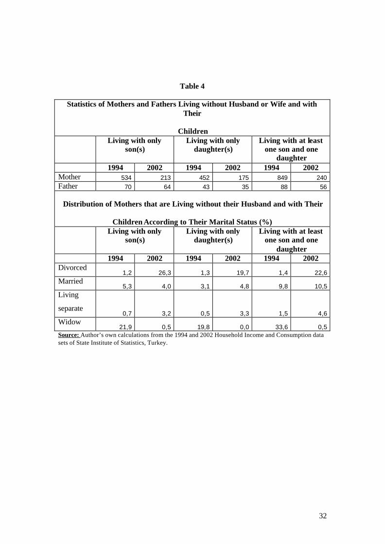
Table 4 presents the distribution of the mothers that are living only with their children

according to their marital status. From the table it seems like in 2002 the number of

the alone parents decreases but this is due to the fact that the 2002 data has less

observations than the 1994 data. In the first part of the table the important thing to

compare is the difference between mothers and fathers. It can be observed that

number of alone fathers is much less than the number of alone mothers in both years.

One of the reasons for this is the fact that the expected age of women is higher than

men, but also it might be concluded that fathers prefer not to raise their children

alone, even if they are divorced with the mother of their children or the mother passed

away, they marry another person that would take care of them.

As the sample of alone fathers is very small and having only father’s effect is

generally insignificant on children’s school attainment, in the second part of the table

only mothers’ distribution is analyzed. The interesting thing about the second part of

the table is the change in reason of being an alone mother between the years 1994 and

2002. In 1994 in general alone mother’s are widows, while in 2002 most of the alone

mothers are divorced women. In recent years there is a substantial increase in divorce

rates in Turkey. This is mostly due to the increase in economic and social freedom of

women.

In 1994 over 70% of the women were alone as their husbands were passed away and

approximately husbands of 20% of women live abroad or in another city. Being

divorced and living separate do not constitute a high proportion of the alone women.

This result is not surprising as in those years although it was legal to get divorced; it

was not practiced as much as today, as it was against the social norms. It can be

concluded that if the mother is the only one who gives the decision about the

education demand, there is a higher probability that the child goes to school.

In 2002 data, it can be observed that more than 60% of the mothers living only with

their children are divorced and over 20% is still married meaning that the father is

working in another city or abroad. The other options like the father is death or the

16

parents decided not to divorce but live separately do not have a high proportion of the

sample. Considering the fact that most of this sample contains divorced mothers it

might be concluded that mothers give more importance to the education of their

children, and higher to their daughters when they have power to decide. Moreover,

20% of the sample contains the families the father of which is working abroad or in

another city. For these we can conclude that the father earns higher in the place that

he works (otherwise he would prefer to stay with his family) and this decreases the

credit constraint on the family. On the other hand in 2002, the estimate of the

coefficient loses its significance for boys in both education levels. This can be due to

the higher responsibility given to the oldest boy as now he is the man of the family or

the fact that boys need more control of their fathers to be in discipline.

Furthermore, it can be observed that the coefficient values for only mother are higher

for 2002 than 1994. This is in accordance with the increase in economic and social

power of women. As discussed above in 1994 in general women were alone as their

husbands were death, but in 2002 if they are alone it is usually their own choice.

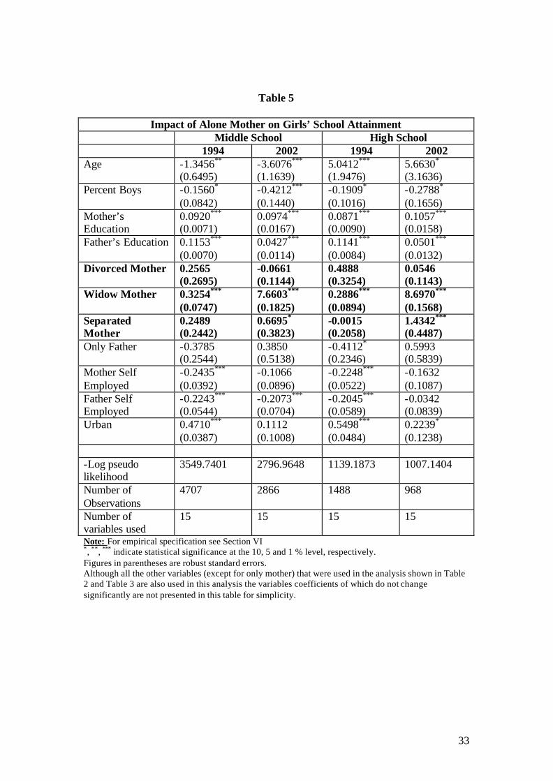
After looking at the overall statistics, a deeper analysis is made to see whether being

divorced, separated or widow has a higher impact on children’s school attainment. In

order to attain the only mother dummy is changed with to other dummies: Divorced,

widow and separated. The same ordered probit regression is run and the results are

presented in Table 5 and Table 6 for girls’ and boys’ school attainment respectively.

As it is the repetition of the previous regression except for the dummies not all

variables are shown in the table, only the ones that are significantly changed relative

to the previous case in at least one of the columns are added for simplification.

In Table 5, it can be observed that divorced mothers do not have any significant effect

on girls’ school attainment. However, there is a high and significant effect of having a

widow mother. Furthermore for 2002 a positive and significant effect for having a

separated mother is also observed, although it is not as high as the impact of widow

mother. In general the analysis for the girls proves that when mothers have power to

decide the girls’ school attainment increases.

17

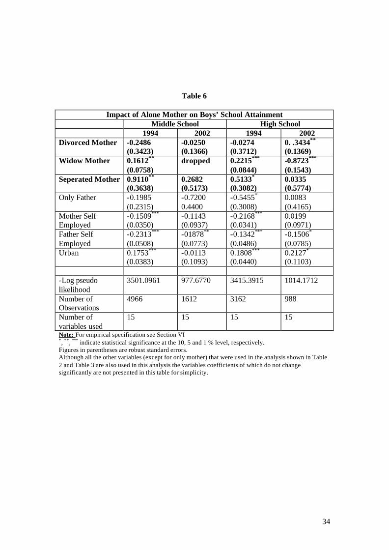
On the other hand Table 6 presents the same analysis for boys’ school attainment. The

interesting about this analysis is the fact that in 2002 divorced mother has a positive

effect on boys’ high school attainment, while the impact of widow mother is negative.

This might be due to the fact that divorced mothers can still get monetary help from

their ex-husbands while widow mothers have to earn on their own. And seeing this

impact on high school attainment might show that the boys start to work earlier

instead of going to school to be able to help their family to survive. On the other hand

widow mother has positive impact on boys’ school attainment in 1994, while it has

negative impact in 2002. This might be due to decrease in living standards in Turkey

after the economic crisis. In 2002 it became more difficult for a family without a

father to survive than in 1994. Lastly the positive effect of having a separated mother

in 1994 loses its significance in 2002. Here another interesting thing is the fact that for

girls, separated mothers do not have any significant impact in 1994 but they start to

have a positive significant impact in 2002. It might be the case that in 2002 separated

mothers decided to care more about their daughters’ education, while in 1994 they

were caring more about their sons’ education. This might be due the increase of

women in labor force in Turkey, so investing in girls’ education also started to bring

higher returns in the future.

VII- Impact of the Extension of Compulsory Education

As discussed before compulsory education in Turkey is extended from 5 years to 8

years in September 1997. Some of its effects might be predicted from the previous

analysis but to be more confident about the impact, in this section some additional

analysis will be made.

a) Summary Statistics

In order to have an overall idea of the middle school enrollment in Turkey, school

enrollment data of State Statistics Institute in Turkey is gathered for the years 1990-

2005. Figures 1 and 2 present the enrollment of both boys and girls in middle

schooling between the years 1990-2005 in urban and rural areas, respectively. After

1997 a sharp increase can be observed in enrollment of both boys and girls in urban

18

areas. Furthermore in rural areas before 1997 there was a decreasing trend of middle

school enrollment of the children, and with extension it started to increase again,

finally coming to its original level of 1990 in 2005. It might be concluded that in

terms of enrollment the extension was more beneficial for the children in rural areas.

Not because it increased a lot the enrollment relative to the beginning of 90’s, but

because it stopped the decreasing trend of middle school enrollment. The number of

schools for this period is presented in Figure 3. Most probably due to the process of

adoption to the new system, after 1999 a decrease in number of middle schools is

observed. The data before 1997 contains the sum of primary and secondary schools,

while after 1997 all schools were obliged to give eight years of education. It might be

the fact that as primary and secondary schools are combined, now one school that was

primary school before and another that was secondary school would be counted as

only one school. After 1997 all schools that give eight years of education are named

as primary schools even if there are two separate schools, and counting them

separately might cause double counting. As a result it might be concluded that the

increase in middle school attainment is not due to an increase in the number of

schools.

Another question would be whether this combination of schools caused any change in

classroom size or students per teacher ratio. Figures 4 and 5 present the classroom

size for urban and rural areas, respectively. While a stable pattern is observed in urban

areas, a sudden increase is seen in the class size of rural areas in 1997 deserves

attention. It might be due to the lack of schools and increase in demand for schools in

rural areas. Figure 6 present that there has not been a substantial change in average

number of students per teacher during the period 1990-2005. On the other hand it is

interesting to observe that in 2005 number of students per teacher in urban areas fall

below the ones in rural areas.

b) Difference in Differences Approach

Concluding that all the increase in school enrollment would also cause the same

increase in graduate rates would be misleading. In order to isolate the impact of the

extension of compulsory education difference in differences method is used.

19

The oldest children that would be affected by the extension would be 17 years old in

2002, and the ones who are 18 years old in 2002 are the youngest ones that are not

exposed to this change in compulsory education. Not to end up with very small

sample size, it is decided to compare children between 16-17 years old with the ones

who are 18-19 years old. Children between 16-17 years old are taken as the treatment

group and the ones that are 18-19 years old are used as control group. 16-17 years old

children in 1994 sample are the ones who were not exposed to the policy change and

the ones in 2002 were affected by the extension in compulsory education. As the

maximum amount of schooling years that could be finished by a 16 years old child is

8 years in 2002, the maximum amount of education is set for 8 years for all age

groups. In this analysis it is important to see whether the extension of compulsory

education increased the mean education level of children towards 8 years. Table 5

presents the results of analysis for boys and girls separately both for urban and rural

areas. In order to calculate the mean values of education of children following OLS

regression are used:

Eduijk = ß1 aftertreat + eijk (7)

Eduijk = ß2 aftercontrol + eijk (8)

Eduijk = ß3 beforetreat + eijk (9)

Eduijk = ß4 beforecontrol + eijk (10)

where i stands for the individual, j presents the gender and k shows the location

(urban or rural). The independent variables are the interaction of two dummy

variables after and treat, which take value 1 for the 2002 data and for 16 and 17 years

old children, respectively. Control is the case when treat dummy takes value zero, and

similarly before is the case when after dummy takes the value zero. The estimated

value of coefficients and their standard errors are shown in Table 7 for all

combinations, ß1 taking the place at the upper left part of the table. In each table the

bold number at the right bottom corner shows the difference in differences estimate.

Contrary to the expectations the results for urban boys and rural girls are negative, but

the difference in differences estimate for the girls living in rural areas is not

significant. Nevertheless it might be concluded that the extension of compulsory

education did not have an impact on all children in the same manner. In this analysis,

20

the exact number of years of education cannot be known as the options in the survey

are 0, 2, 5 and 8 years, but it is the same for both years and both groups, so this should

not affect the results. The results show that this program had a negative effect on

education level of the boys in urban area, while it affected positively the girls in the

cities. This is rather a surprising result after observing the increase in enrollment rates

in the previous section. It might be concluded that extension of compulsory education

did no have any significant effect in graduation rates in rural areas, mostly due to high

drop out rates. In the first box in Table 7 it can be observed that the simple difference

between the years 2002 and 1994 is positive for both treatment and control groups for

the boys in urban area. So there is an improvement in 2002 relative to 1994, but this

improvement is more for control group than for treatment group, so there might be

other changes occurred in this period that have impact on school attainment. Both this

and the fact that difference in difference estimate being significant at only 10% level

make it dubious whether this effect is only because of the application of this policy.

In order to isolate the impact of extension of compulsory education, the following

OLS regression is run:

Eduij = ß0 + ß1Xij + ß2 Afterij + ß3 Treatij + ß4 Aftertreat ij + eij (11)

where i stands for the individual and j for the gender. X is the vector of individual and

family characteristics same as used in ordered probit estimates. After is the dummy

that takes value one for the 2002 observations, while treat is the dummy for 16-17

years old children. Aftertreat is the interaction of these two dummies, meaning

coefficient estimate for ß4 shows the difference in differences estimate. This

regression is run three times: For boys, for girls, and for pooled sample of both boys

and girls. The results are shown in Table 8.

The results present that after controlling for individual and family characteristics the

extension of compulsory education did not have any significant effect on boys’

education level, while it had a positive impact on girls’ education. But from the

pooled data results it can be concluded that this policy did not have any significant

impact on education level in general. Although it increased the enrollment rates, this

increase is not followed by an increase in graduation rates.

21

c) Impact on Household Labor Force

Extension of compulsory education may also affect the labor force combination of the

household. In this section first whether mothers have started working after this policy

change is analyzed by using difference in differences approach in a probit estimate.

Households that have at least one child between 16-17 years old are taken as

treatment group and the ones that have at least one child between 18-19 years old are

taken as control group. The families that have a child both at the age of 16-17 and 18-

19 are excluded from the sample. The following probit regression is used:

Pi = ß0 + ß1Xi+ ß2Treati + ß3Afteri + ß4AfterTreat i + ei (12)

where Pi is the dummy variable which takes the value 1 when mother is working, X is

the vector of household characteristics such as the mother’s and father’s education,

the ages of mother and father, the squared terms of mother’s and father’s age divided

by 100, two dummies that take the value one if the mother is self employed and father

is self employed, the dummy that shows if the father is working in the public sector,

the dummy that represents whether the father has any second job, the dummy that

takes the value one if the household is engaged in agricultural activities, the dummy

that takes the value one if at least one child in the household is working, variables that

represent the number of children between the age zero and six, seven and fifteen,

sixteen and seventeen, eighteen and nineteen, the average education level of the girls

and boys in the household. The dummy variable Treat takes the value one for the

treatment group, in the same manner dummy variable After takes the value one for the

year 2002 and AfterTreat is the interaction term of both. The results are shown in

Table 9.

As expected the results show that the higher educated mothers have higher probability

to work. On the other hand as husband’s education level increases the probability that

the wife works decreases. This might be due to the fact that with higher education

level husband is earning good enough not to need his wife’s work. Another important

result is the fact that wives of men that have an additional job have a higher

probability to work. This means that firstly men try their best to supply all household

needs by themselves by even working in two jobs. This also shows that in general

22

women work because of economic reasons, otherwise it is not a common issue in

Turkey except for the rural areas. In the families that are engaged in agricultural

sector the probability that the mother works is higher. Expectedly also the existence of

a working child in the family increases the probability of mothers’ work. Most

probably children are forced to work if the income of both parents is not enough to

survive the family. Furthermore number of children between 0-6 years old decreases

the probability that that the mother works, most probably because they need care of

the mother. Sometimes the cost of finding someone to take care of the child might be

higher than the mother would earn if she works. Another factor that decreases the

probability of mothers’ working is the average education of the boys in the family. As

boys get more educated they might work in better jobs and help the family income by

earning more.

The most important result of this analysis is the fact that the extension of compulsory

education did not have any significant effect on mothers’ working, as the coefficient

estimate for ß4 is not significant. The same analysis is repeated also for father getting

an additional work and again no significant result is found, so the results are not

presented here. Finally it is checked whether this policy affected the working hours in

the family by using the following OLS regression:

Workinghouri = ß0 + ß1Xi+ ß2Treati + ß3Afteri + ß4AfterTreat i + ei (13)

where Workinghour represents the total hours of work in the household, and the

definition of the other variables are the same as in the previous analysis that is done

for mothers. The results are shown in Table 8.

The results present that as the education level of parents increases working hour

decreases, which is expected as high educated would have a higher wage and a better

job, and do not have to work for extra hours. Also as parents’ age increases, working

hours increase, perhaps it is due to the fact that as the age increases the position at the

work upgrades and the amount of responsibility increases. This idea can be also

supported by the fact that having a self employed father increases the working hours.

When someone owns the job he feels higher responsibility and also by increasing his

working hours he can increase his income. On the other hand having a father working

23

in public sector decreases the working hours in the household as in the public sector

the working time is fixed and it is not as many hours as in private sector. Households

that work on their farms or doing some kind of agricultural work tend to spend more

time working. As expected total number of working hours increase in the families in

which the mother works. There is also a positive relationship between income and the

total number of hours worked. Higher income families tend to work more hours,

probably they have higher income as they work more. In cities households tend to

work less. The number of children below 15 years old decrease the total hour of work

both because they need care and also they do not work, while children between 16-19

years old increase the total hour of work as they might be also start working to help

their family. As the average of the education of the girls in the family increases the

total working hours decrease. This might be because of two reasons. First might be

the fact that instead of working, girls go to school. Second reason might be the case

that higher income families have higher tendency to send their daughters to school

and they do not work too many hours as they have a high wealth. The most important

result of this analysis is the coefficient estimate of ß4, which shows the difference in

differences estimate. It is positive and significant, meaning that extension of

compulsory education forced the credit constraint families to work for more hours.

Combining with the previous analysis it can be concluded that income constraint

families in Turkey prefer to increase their working hours instead of having working

mothers.

d) Impact on Child Labor

One of the aims of the extension of the compulsory education was to keep the

children at school for three more years, so it is important to evaluate if this policy

decreased the child labor. The dummy child labor takes the value one if the child is

less than 16 years old and worked at least for one month during the survey year. As in

the previous section a probit estimate is formed and difference in differences

methodology is used. The following probit regression is used:

ChildLabori = ß0 + ß1Xi+ ß2Treati + ß3Afteri + ß4AfterTreat i + ei (14)

24

where the definition of the variables is the same as in the previous section. The results

are presented in Table 11.

The results show that the reason of children’s work is mostly income oriented. This is

proved by the fact that the probability of working child decreases with the income

level. Interestingly enough it does not depend on parents’ education level. Having a

self employed father decreases the probability to work. Most probably even if the

children work at their father’s place they are no t reported as working. Usually parents

do not count as a job if the child is working with them, so children working in the

farm or working place of their parents are not reported as a child labor in the survey.

Another factor that decreases the probability of child labor is having a father that

works in public sector, as working in public sector is a relatively safer job and also

having a child, they receive transfer. Having a father who has a second job increases

the probability that the child works, most probably because of economic reasons.

Even the father’s having a second job is not enough so that the children also work.

Having a working mother has a very significant negative effect on the probability of

child labor. Mothers prefer to work themselves instead of letting their child work. In

urban locations there is a lower probability that the children work, most probably

because there are more strict controls about child labor in the cities. The results show

that higher education of boys decreases the probability of child labor while the

coefficient estimate of average education of girls is not significant. This is due the fact

that there are not many reported female child labor in the survey. In the data set it is

observed that in general boys are working when they are a child, but in reality girls

are also working. But usually girls do domestic work and they do not earn money, so

their work is not reported. ß4 shows the difference in differences estimate for the

effect of extension of compulsory education on child labor. It is both negative and

significant at 5% level. It might be concluded that the extension of compulsory

education was successful in decreasing the child labor, which is consistent with the

simulation results of Dayioglu (2005).

25

VIII- Conclusion

This paper examines the main determinants of school attainment in Turkey and the

effect of the extension of compulsory education on the school attainment. In order to

observe the determinants of school attainment ordered probit models are formed for

middle and high schooling for the years 1994 and 2002. Education of parents,

household income, and number of children in the household seem to be main

determinants for both boys and girls in both years, although the marginal effect is

different for genders. These determinants affect girls’ attainment more than boys’ in

both years. While girls are more negatively affected by the number of the boys in the

household, boys are influenced negatively by having a self employed father. Living in

urban region lost its positive significance, which it had in 1994, in 2002 for middle

schooling. It is also proved that when mothers have power to decide they give more

importance to their children’s education. It might be concluded that income growth,

increase in parents’ education and fertility control contribute positively to children’s

school attainment, and their positive effect will be higher for girls than boys. Turkey’s

gini coefficient was 0.383 in 2005, higher than all EU countries. The results of this

study present that income inequality would negatively affect the school attainment so

if Turkey wants to reach the universal school attainment it should take care of this

problem. In Turkey legally abortion is free and in the statistics it is observed that

women are aware of pregnancy controls4, but from the population growth we

understand that they are not applied in practice5. High number of children in the

household decreases the probability of school attainment, and education is an

important factor in controlling the fertility, so there is a dual causality here, which can

be solved by increasing the awareness of parents about this fact.

In order to see the impact of extension of compulsory education first the overall

statistics are checked. Although it seem like the extension increased the overall

enrollment rate, the further analysis prove that because of the drop outs this policy has 3 In 1994 the gini coefficient was 0.49 and became 0.44 in 2002. For the years 2005 and 2006 it stayed stable at 0.38 Turkish Statistical Institute Population and Growth Indicators http://nkg.tuik.gov.tr/ 4 The percentage of women who knows the ways to control pregnancy is 99.1 in 1993 and 99.8 in 2003. Turkish Statistical Institute Population and Growth Indicators http://nkg.tuik.gov.tr/ 5 Number of children per women shows a decreasing trend since 1990 but trend slows down after 2000. In 2001 the average number of children per woman is 2.25 and it becomes 2.19 in 2005 and stays the same in 2006.

26

not been as effective as one would expect. Only the girls living in the cities seem to be

positively effected by the extension of compulsory education in terms of school

attainment, and when the pooled data is concerned it does not seem to have any

significant effect. The extension of compulsory education may also affect the labor

force combination of the households. In order to understand this, difference in

differences methodology is used by taking the 16-17 years old children as treatment

group and 18-19 years old children as control group. The results show that this policy

increased the total working hours in the households, but it did not have any effect on

the probability that the mother starts working or father gets an additional job. On the

other hand it had a positive effect on child labor by decreasing the probability of child

labor in the households. This study shows that in Turkey when a household needs

extra income the first way they choose is to increase the working hours of the head of

the household rather than letting mothers work. Furthermore policies that would keep

children more in school would decrease the child labor amount in Turkey

substantially.

Having a stable economy seems to be one of the most important factors to be

sustained in order to have a universal school attainment. Furthermore this study shows

that having high enrollment rate does not necessary bring high graduation rate. After

sustaining the high enrollment rate precautions should be taken to prevent dropouts,

especially in rural areas. This might be done by taking account of the factors that

influence the school attainment in Turkey, which are analyzed in the first part of this

paper. Furthermore, these results might be important when shaping the future policies,

as the new government of Turkey is planning to extend the compulsory education to

12 years in 2012.

27

References

Becker, G.S. (1975). Human Capital: A Theoretical and Empirical Analysis with

Special Reference to Education, Second Edition, New York: National Bureu of

Economic Research.

Black, S.E, Devereux, P.J, and K. G. Salvanes (2004). “Fast Times at Ridgemont

High? The Effect of Compulsory Schooling Laws on Teenage Births”, IZA

Discussion Papers, No:1416.

Conelly, R., Zheng, Z. (2002). “Determinants of School Enrollment and Completion

of 10 to 18 Years Old in China”, Economics of Education Review, 22 p: 379-388.

Dayioglu, M. (2005). “Patterns of Change in Child Labor and Schooling in Turkey:

The Impact of Compulsory Schooling”, Oxford Development Studies, 33(2) p:195-

210.

Dulger, I. (2004). “Turkey: Rapid Coverage for Compulsory Education- The 1997

Basic Education Program”, Case Studies in Scaling up Poverty Reduction, World

Bank.

Holmes, J. (1999). “Measuring the Determinants of School Completion in Pakistan:

Analysis of censoring and Selection Bias”, Yale University Economic Growth

Center, Center Discussion Paper No: 794.

Ilon, L., Moock, P. (1991). “School Attributes, Household Chracteristics, and

Demand fro Schooling: A Case Study of Rural Peru”, International review of

Education, 37(4) p: 429-451.

King, E., Lillard, L. (1983). “Determinants of Schooling Attainment and Enrollment

Rates in the Philippines”, Rand Report, N-1962-AID.

King, E., Lillard, L. (1987). “Education Policy and Schooling Attainment in Malaysia

and the Philippines”, Economics of Education Review, 6(2) p: 167-181.

King, E.M., Hill, M.A. (1993). Women’s Education in Developing Countries:

Barriers, Benefits and Policies, Baltimore: The John Hopkins University Press for

the World Bank.

Knight, J., Song, L. (2000). “Differences in Educational Access in Rural China”,

University of Oxford Working Paper, Department of Economics, University of

Oxford.

Lleras-Muney, A. (2005). “The Relationship Between Education and Adult Mortality

in the United States”, Review of Economic Studies, 72 p: 189-221.

28

Mcintosh, S. (2001). “The Demand for Post-Compulsory Education in Four European

Countries”, Education Economics, 9(1) p: 71-90.

Oreopoulos, P. (2006). “The Compelling Effects of Compulsory Schooling: Evidence

from Canada”, Canadian Journal of Economics, 39(1) p: 22-52.

Schultz, T.W (1963). The Economic Value of Education, New York: Columbia

University Express.

Schultz, T.W. (1974). Economics of the Family, Chicago: University Chicago

Express.

Schultz, T.W. (1995b). “The Economics of Women’s Schooling” in The Politics of

Women’s Schooling: Perspectives from Asia, Africa and Latin America, eds J.K.

Conway and S.C. Bourque. Ann Arbor: The University of Michigan Press.

Tansel, A. (2002). “Determinants of School Attainment of Boys and Girls in Turkey:

Individual, Household and Community Factors”, Economics of Education Review, 21

p: 455 – 470.

Tansel, A. (2005). “Public-Private Employment Choice, Wage Differentials, and

Gender in Turkey”, Economic Development and Cultural Change, 53(2) p: 453-477.

Wigley, A.A, Wigley, S. (2005). “Basic Education and Capability Development in

Turkey”, forthcoming in Education in Turkey, Arnd-Michael Nohl ed. Munster and

New York: Waxmann.

29

Table 1

Average Years of Schooling for Boys, Girls and Parents,

Age 16-20, Turkey, 1994

Boys (average

years)

Girls (average

years)

Fathers

(average years)

Mothers

(average years)

Age 1994 2002 1994 2002 1994 2002 1994 2002

16 6.84 7.13 6.03 6.68 5.21 6.08 3.37 3.71

17 7.37 7.77 6.38 6.98 5.44 5.85 3.56 3.97

18 7.55 8.31 6.68 7.49 5.14 5.91 3.42 3.73

19 7.76 8.74 7.21 7.97 5.04 5.90 3.42 3.61

20 7.96 9.03 6.80 7.81 4.80 5.60 3.32 3.53

Total 7.44 8.07 6.53 7.32 5.16 5.89 3.43 3.73

Source: Author’s own calculations from the 1994 and 2002 Household Income and Consumption data sets of State Institute of Statistics, Turkey.

Average Years of Schooling for Boys, Girls and Parents,

Age 16-20, Turkey, 1994*

Male(average

years)

Female

(average years)

Fathers

(average years)

Mothers

(average years)

Age 1994 2002 1994 2002 1994 2002 1994 2002

16 6.78 7.10 5.97 6.59 5.21 6.08 3.37 3.71

17 7.28 7.75 6.26 6.84 5.44 5.85 3.56 3.97

18 7.47 8.25 6.35 7.13 5.14 5.91 3.42 3.73

19 7.64 8.75 6.56 7.46 5.04 5.90 3.42 3.61

20 7.80 9.04 5.96 6.91 4.80 5.60 3.32 3.53

Total 7.35 8.06 6.20 6.97 5.16 5.89 3.43 3.73

Source: Author’s own calculations from the 1994 and 2002 Household Income and Consumption data sets of State Institute of Statistics, Turkey. * All people between 16-20 years are taken into consideration even if they left their initial household and formed their own one.

30

Table 2

Ordered Probit Estimates of Middle Schooling Ages 16-19

Variables Boys Girls

Year 1994 2002 1994 2002 Age 0.5345

(0.6331) -0.4200 (1.2367)

-1.3523** (0.6485)

-3.6792*** (1.1647)

Age2 -0.0162 (0.0181)

0.0107 (0.0352)

0.0391** (0.0186)

0.1029*** (0.0333)

Percent Boys -0.1689** (0.0841)

-0.4262*** (0 .1437)

Percent Girls -0.0196 (0.0840)

0.0869 (0.1584)

No of Children -0.0788*** (0.0109)

-0.0865*** (0.0216)

-0.1699*** (0.0104)

-0.1971*** (0.0228)

Log Expenditure 0.0721*** (0.0238)

0.2171*** (0.0743)

0.1923*** (0.0246)

0.2628*** (0.0643)

Mother’s Education 0.0465*** (0.0068)

0.0720*** (0.0137)

0.0884*** (0.0070)

0.0923*** (0.0171)

Father’s Education 0.1013*** (0.0073)

0.0797*** (0.0174)

0.1191*** (0.0072)

0.0551*** (0.0129)

Only Mother 0.3237*** (0.1032)

0.1422 (0.1750)

0.3283*** (0.0969)

0.4032** (0.1580)

Only Father -0.1855 (0.2314)

-0.7050 (0.4405)

-0.3420 (0.2534)

0.3939 (0.5120)

Mother Self Employed 0.0323 ( -4.16 )

-0.1153 (0.0929)

-0.1973*** (0.0350)

-0.1110 (0.0889)

Father Self Employed -0.2179 ***

(0.0502) -0.1715** (0.0791)

-0.2389*** (0.0551)

-0.1653**

(0.0741) Urban 0.1702***

(0.0383) -0.0060 (0.1089)

0.4713*** (0.0386)

0.1172 (0.0999)

-Log pseudo likelihood 3502.3363 977.55375 3554.5449 1137.883 Number of Observations 4966 1612 4707 1488 Prob(education=middle school)

0.6067 0.7680 0.4240

0.6095

Note: For empirical specification see Section V *, **, *** indicate statistical significance at the 10, 5 and 1 % level, respectively. Figures in parentheses are robust standard errors.

31

Table 3

Ordered Probit Estimates of High Schooling Ages 18-20

Variables Boys Girls

Year 1994 2002 1994 2002 Age -0.7556

(1.7191) 0.2276 (3.1064)

5.1511*** (1.9457)

5.6038* (3.1657)

Age2 0.0226 (0.0453)

-0.0009 (0.0821)

-0.1341*** (0.0513)

-0.1458* (0.0835)

Percent Boys -0.1999** (0.1013)

-0.2695 (0 .1647)

Percent Girls 0.0620 (0.0943)

0.1044 (0.1625)

No of Children -0.0700*** (0.0127)

-0.0817*** (0.0230)

-0.1715*** (0.0129)

-0.2156*** (0.0275)

Log Expenditure 0.1230*** (0.0267)

0.1869** (0.0786)

0.1488*** (0.0321)

0.3117*** (0.0721)

Mother’s Education 0.0518*** (0.0071)

0.0682*** (0.0142)

0.0855*** (0.0090)

0.1005*** (0.0159)

Father’s Education 0.0874*** (0.0075)

0.0668*** (0.0132)

0.1175***

(0.0086) 0.0627*** (0.0156)

Only Mother 0.3126*** (0.1107)

0.0914 (0.1744)

0.3454*** (0.1137)

0.5378*** (0.1742)

Only Father -0.5282* (0.2993)

-0.0129 (0.4222)

-0.3816 (0.2342)

0.5837 (0.5999)

Mother Self Employed -0.1969***

(0.0323) 0.0422 (0.0974)

-0.1894***

(0.0463) -0.1731 (0.1080)

Father Self Employed -0.1317***

(0.0479) -0.1724** (0.0805)

-0.2126*** (0.0562)

-0.0172

(0.0892) Urban 0.1721***

(0.0441) 0.2201** (0.1096)

0.5500*** (0.0484)

0.2291*

(0.1232) -Log pseudo likelihood 3416.1655 1017.7223 2799.0096 1007.4001 Number of Observations

3162 988 2866 968

Prob(education=high school)

0.3707 0.4960 0.3193 0.6032

Note: For empirical specification see Section V *, **, *** indicate statistical significance at the 10, 5 and 1 % level, respectively. Figures in parentheses are robust standard errors.

32

Table 4

Statistics of Mothers and Fathers Living without Husband or Wife and with Their

Children

Living with only son(s)

Living with only daughter(s)

Living with at least one son and one

daughter 1994 2002 1994 2002 1994 2002

Mother 534 213 452 175 849 240 Father 70 64 43 35 88 56

Distribution of Mothers that are Living without their Husband and with Their

Children According to Their Marital Status (%)

Living with only son(s)

Living with only daughter(s)

Living with at least one son and one

daughter 1994 2002 1994 2002 1994 2002

Divorced 1,2 26,3 1,3 19,7 1,4 22,6

Married 5,3 4,0 3,1 4,8 9,8 10,5

Living

separate 0,7 3,2 0,5 3,3 1,5 4,6

Widow 21,9 0,5 19,8 0,0 33,6 0,5

Source: Author’s own calculations from the 1994 and 2002 Household Income and Consumption data sets of State Institute of Statistics, Turkey.

33

Table 5

Impact of Alone Mother on Girls’ School Attainment Middle School High School 1994 2002 1994 2002 Age -1.3456**

(0.6495) -3.6076*** (1.1639)

5.0412***

(1.9476) 5.6630* (3.1636)

Percent Boys -0.1560* (0.0842)

-0.4212*** (0.1440)

-0.1909* (0.1016)

-0.2788* (0.1656)

Mother’s Education

0.0920***

(0.0071) 0.0974*** (0.0167)

0.0871*** (0.0090)

0.1057*** (0.0158)

Father’s Education 0.1153*** (0.0070)

0.0427*** (0.0114)

0.1141*** (0.0084)

0.0501*** (0.0132)

Divorced Mother 0.2565 (0.2695)

-0.0661 (0.1144)

0.4888 (0.3254)

0.0546 (0.1143)

Widow Mother 0.3254*** (0.0747)

7.6603*** (0.1825)

0.2886*** (0.0894)

8.6970*** (0.1568)

Separated Mother

0.2489 (0.2442)

0.6695* (0.3823)

-0.0015 (0.2058)

1.4342*** (0.4487)

Only Father -0.3785 (0.2544)

0.3850 (0.5138)

-0.4112* (0.2346)

0.5993 (0.5839)

Mother Self Employed

-0.2435*** (0.0392)

-0.1066 (0.0896)

-0.2248*** (0.0522)

-0.1632 (0.1087)

Father Self Employed

-0.2243*** (0.0544)

-0.2073*** (0.0704)

-0.2045*** (0.0589)

-0.0342 (0.0839)

Urban 0.4710*** (0.0387)

0.1112 (0.1008)

0.5498***

(0.0484) 0.2239* (0.1238)

-Log pseudo likelihood

3549.7401 2796.9648 1139.1873 1007.1404

Number of Observations

4707 2866 1488 968

Number of variables used

15 15 15 15

Note: For empirical specification see Section VI *, **, *** indicate statistical significance at the 10, 5 and 1 % level, respectively. Figures in parentheses are robust standard errors. Although all the other variables (except for only mother) that were used in the analysis shown in Table 2 and Table 3 are also used in this analysis the variables coefficients of which do not change significantly are not presented in this table for simplicity.

34

Table 6

Impact of Alone Mother on Boys’ School Attainment Middle School High School 1994 2002 1994 2002 Divorced Mother -0.2486

(0.3423) -0.0250 (0.1366)

-0.0274 (0.3712)

0. .3434**

(0.1369) Widow Mother 0.1612**

(0.0758) dropped 0.2215***

(0.0844) -0.8723*** (0.1543)

Seperated Mother 0.9110** (0.3638)

0.2682 (0.5173)

0.5133* (0.3082)

0.0335 (0.5774)

Only Father -0.1985 (0.2315)

-0.7200 0.4400

-0.5455* (0.3008)

0.0083 (0.4165)

Mother Self Employed

-0.1509***

(0.0350) -0.1143 (0.0937)

-0.2168***

(0.0341) 0.0199 (0.0971)

Father Self Employed

-0.2313*** (0.0508)

-01878** (0.0773)

-0.1342*** (0.0486)

-0.1506* (0.0785)

Urban 0.1753***

(0.0383) -0.0113 (0.1093)

0.1808*** (0.0440)

0.2127* (0.1103)

-Log pseudo likelihood

3501.0961 977.6770 3415.3915 1014.1712

Number of Observations

4966 1612 3162 988

Number of variables used

15 15 15 15

Note: For empirical specification see Section VI *, **, *** indicate statistical significance at the 10, 5 and 1 % level, respectively. Figures in parentheses are robust standard errors. Although all the other variables (except for only mother) that were used in the analysis shown in Table 2 and Table 3 are also used in this analysis the variables coefficients of which do not change significantly are not presented in this table for simplicity.

35

Table 7

Boys’ Education (Urban) Treatment Group:16-17

years old Control Group: 18-19

years old Difference

After:2002 7.1299***

(0.2379) 7.1974***

(0.2684) -0.0675 (0.0900)

Before:1994 6.9086***

(0.1275) 6.7834***

(0.1561) 0.1252** (0.0580)

Difference 0.2213*** (0.0745)

0.4140*** (0.0790)

-0.1927* (0.1093)

Boys’ Education (Rural) Treatment Group:16-17

years old Control Group: 18-19

years old Difference

After:2002 7.11129***

(0.5778) 6.8241***

(0.6243) 0.2888

(0.2222) Before:1994 6.4522***

(0.1728) 6.2881***

(0.2005) 0.1641

(0.0907) Difference 0.6607***

(0.1715) 0.5360*** (0.1828)

0.1247 (0.2508)

Girls’ Education (Urban) Treatment Group:16-17

years old Control Group: 18-19

years old Difference

After:2002 6.6609***

(0.2337) 6.4618***

(0.2625) 0.1991* (0.1205)

Before:1994 6.2454***

(0.1252) 6.3565***

(0.1518) -0.1111 (0.0734)

Difference 0.4155*** (0.0938)

0.1053 (0.1023)

0.3102** (0.1392)

Girls’ Education (Rural) Treatment Group:16-17

years old Control Group: 18-19

years old Difference

After:2002 5.9661***

(0.4969) 6.0526***

(0.5577) -0.0865 (0.3185)

Before:1994 5.1406***

(0.1433) 5.0156***

(0.1863) 0.1250

(0.1073) Difference 0.8255***

(0.2072) 1.0370*** (0.2283)

-0.2115 (0.3091)

Source: Author’s own calculations from the 1994 and 2002 Household Income and Consumption data sets of State Institute of Statistics, Turkey. Note: For empirical specification see Section VI I b *, **, *** indicate statistical significance at the 10, 5 and 1 % level, respectively.

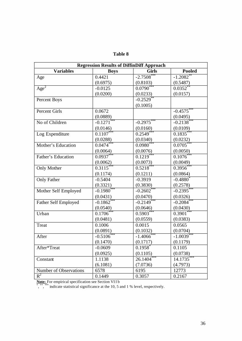
36

Table 8

Regression Results of DiffinDiff Approach Variables Boys Girls Pooled

Age 0.4421 (0.6975)

-2.7508*** (0.8103)

-1.2082** (0.5487)

Age2 -0.0125 (0.0200)

0.0790*** (0.0233)

0.0352** (0.0157)

Percent Boys -0.2529** (0.1005)

Percent Girls 0.0672 (0.0889)

-0.4575*** (0.0495)

No of Children -0.1271*** (0.0146)

-0.2975*** (0.0160)

-0.2138*** (0.0109)

Log Expenditure 0.1107***

(0.0288) 0.2549*** (0.0340)

0.1835*** (0.0232)

Mother’s Education 0.0474*** (0.0064)

0.0980*** (0.0076)

0.0705*** (0.0050)

Father’s Education 0.0937***

(0.0062) 0.1219*** (0.0073)

0.1076*** (0.0049)

Only Mother 0.3115***

(0.1174) 0.5218*** (0.1211)

0.3956*** (0.0864)

Only Father -0.5404

(0.3321) -0.3919 (0.3830)

-0.4880* (0.2578)

Mother Self Employed -0.1980*** (0.0431)

-0.2602*** (0.0470)

-0.2395*** (0.0326)

Father Self Employed -0.1862*** (0.0540)

-0.2149*** (0.0646)

-0.2084*** (0.0430)

Urban 0.1706*** (0.0481)

0.5903*** (0.0559)

0.3901*** (0.0383)

Treat 0.1006 (0.0891)

0.0015 (0.1032)

0.0565 (0.0704)

After -0.5106*** (0.1470)

-1.4066*** (0.1717)

-1.0039*** (0.1179)

After*Treat -0.0609 (0.0925)

0.1958* (0.1105)

0.1105 (0.0738)

Constant 1.1138 (6.1081)

26.1404*** (7.0736)

14.1735*** (4.7973)

Number of Observations 6578 6195 12773 R2 0.1449 0.3057 0.2167 Note: For empirical specification see Section VI I b *, **, *** indicate statistical significance at the 10, 5 and 1 % level, respectively.

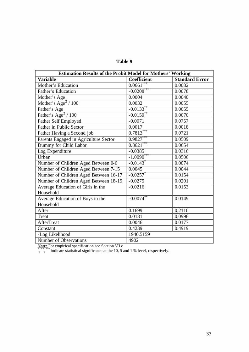
37

Table 9

Estimation Results of the Probit Model for Mothers’ Working Variable Coefficient Standard Error Mother’s Education 0.0661*** 0.0082 Father’s Education -0.0208*** 0.0078 Mother’s Age 0.0004 0.0040 Mother’s Age2 / 100 0.0032 0.0055 Father’s Age -0.0133** 0.0055 Father’s Age2 / 100 -0.0159** 0.0070 Father Self Employed -0.0071 0.0757 Father in Public Sector 0.0017 0.0018 Father Having a Second job 0.7813*** 0.0721 Parents Engaged in Agriculture Sector 0.9827*** 0.0509 Dummy for Child Labor 0.8621*** 0.0654 Log Expenditure -0.0385 0.0316 Urban -1.0090*** 0.0506 Number of Children Aged Between 0-6 -0.0143* 0.0074 Number of Children Aged Between 7-15 0.0045 0.0044 Number of Children Aged Between 16-17 -0.0257* 0.0154 Number of Children Aged Between 18-19 -0.0275 0.0201 Average Education of Girls in the Household

-0.0216 0.0153

Average Education of Boys in the Household

-0.0074** 0.0149

After 0.1699 0.2110 Treat 0.0181 0.0996 AfterTreat 0.0046 0.0177 Constant 0.4239 0.4919 -Log Likelihood 1940.5159 Number of Observations 4902 Note: For empirical specification see Section VII c *, **, *** indicate statistical significance at the 10, 5 and 1 % level, respectively.

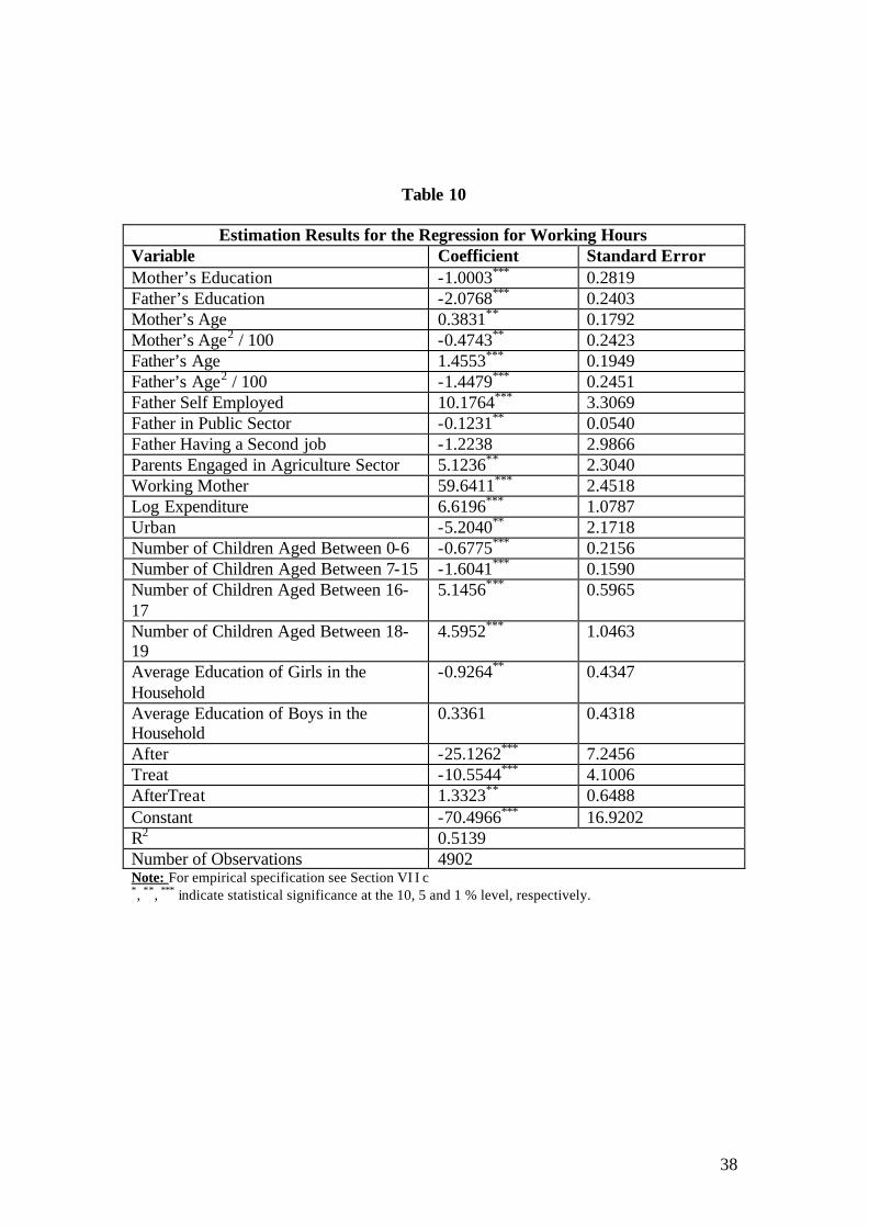
38

Table 10

Estimation Results for the Regression for Working Hours Variable Coefficient Standard Error Mother’s Education -1.0003*** 0.2819 Father’s Education -2.0768*** 0.2403 Mother’s Age 0.3831** 0.1792 Mother’s Age2 / 100 -0.4743** 0.2423 Father’s Age 1.4553*** 0.1949 Father’s Age2 / 100 -1.4479*** 0.2451 Father Self Employed 10.1764*** 3.3069 Father in Public Sector -0.1231** 0.0540 Father Having a Second job -1.2238 2.9866 Parents Engaged in Agriculture Sector 5.1236** 2.3040 Working Mother 59.6411*** 2.4518 Log Expenditure 6.6196*** 1.0787 Urban -5.2040** 2.1718 Number of Children Aged Between 0-6 -0.6775*** 0.2156 Number of Children Aged Between 7-15 -1.6041*** 0.1590 Number of Children Aged Between 16-17

5.1456*** 0.5965

Number of Children Aged Between 18-19

4.5952*** 1.0463

Average Education of Girls in the Household

-0.9264** 0.4347

Average Education of Boys in the Household

0.3361 0.4318

After -25.1262*** 7.2456 Treat -10.5544*** 4.1006 AfterTreat 1.3323** 0.6488 Constant -70.4966*** 16.9202 R2 0.5139 Number of Observations 4902 Note: For empirical specification see Section VI I c *, **, *** indicate statistical significance at the 10, 5 and 1 % level, respectively.

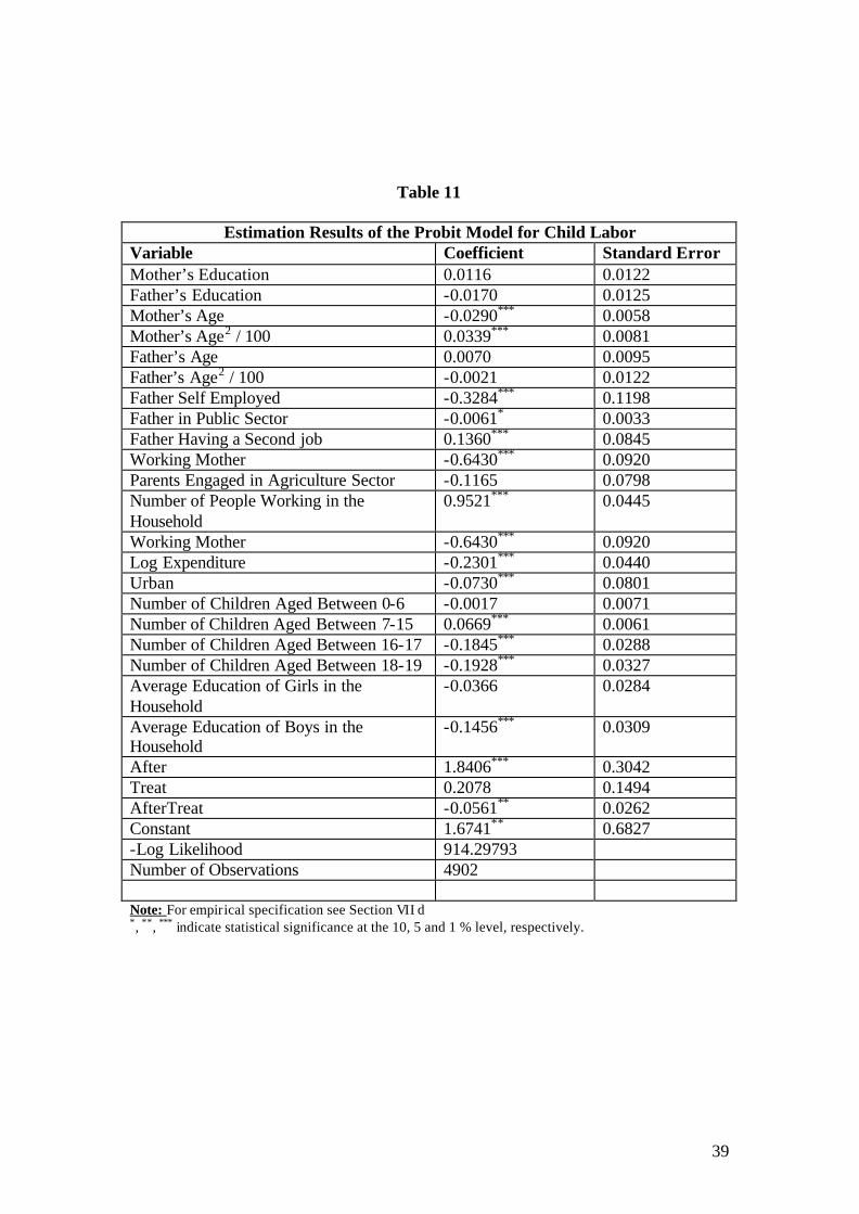
39

Table 11

Estimation Results of the Probit Model for Child Labor Variable Coefficient Standard Error Mother’s Education 0.0116 0.0122 Father’s Education -0.0170 0.0125 Mother’s Age -0.0290*** 0.0058 Mother’s Age2 / 100 0.0339*** 0.0081 Father’s Age 0.0070 0.0095 Father’s Age2 / 100 -0.0021 0.0122 Father Self Employed -0.3284*** 0.1198 Father in Public Sector -0.0061* 0.0033 Father Having a Second job 0.1360*** 0.0845 Working Mother -0.6430*** 0.0920 Parents Engaged in Agriculture Sector -0.1165 0.0798 Number of People Working in the Household

0.9521*** 0.0445

Working Mother -0.6430*** 0.0920 Log Expenditure -0.2301*** 0.0440 Urban -0.0730*** 0.0801 Number of Children Aged Between 0-6 -0.0017 0.0071 Number of Children Aged Between 7-15 0.0669*** 0.0061 Number of Children Aged Between 16-17 -0.1845*** 0.0288 Number of Children Aged Between 18-19 -0.1928*** 0.0327 Average Education of Girls in the Household

-0.0366 0.0284

Average Education of Boys in the Household

-0.1456*** 0.0309

After 1.8406*** 0.3042 Treat 0.2078 0.1494 AfterTreat -0.0561** 0.0262 Constant 1.6741** 0.6827 -Log Likelihood 914.29793 Number of Observations 4902 Note: For empirical specification see Section VII d *, **, *** indicate statistical significance at the 10, 5 and 1 % level, respectively.

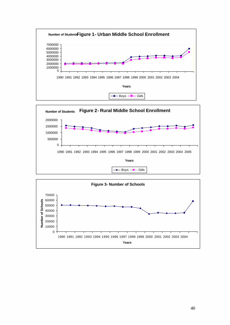
40

Figure 3- Number of Schools

0

10000

20000

30000

40000

50000

60000

70000

1990 1991 1992 1993 1994 1995 1996 1997 1998 1999 2000 2001 2002 2003 2004

Years

Num

ber

of S

choo

ls

Figure 1- Urban Middle School Enrollment

0 1000000 2000000 3000000 4000000 5000000 6000000 7000000

1990 1991 1992 1993 1994 1995 1996 1997 1998 1999 2000 2001 2002 2003 2004

Years

Number of Students

Boys Girls

Figure 2- Rural Middle School Enrollment

0 500000

1000000 1500000 2000000

1990 1991 1992 1993 1994 1995 1996 1997 1998 1999 2000 2001 2002 2003 2004 2005

Years

Number of Students

Boys Girls

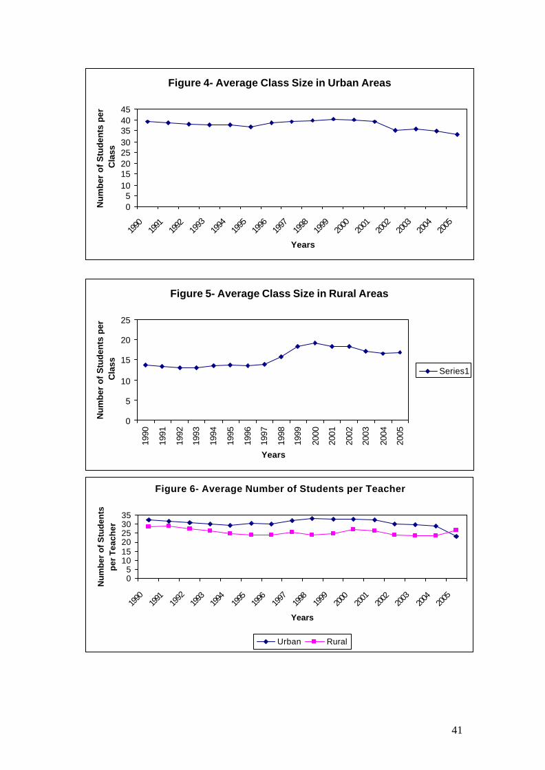
41

Figure 4- Average Class Size in Urban Areas

05

1015202530354045

1990

1991

1992

1993

1994

1995

1996

1997

1998

1999

2000

2001

2002

2003

2004

2005

Years

Nu

mb

er o

f S

tud

ents

per

C

lass

Figure 5- Average Class Size in Rural Areas

0

5

10

15

20

25

1990

1991

1992

1993

1994

1995

1996

1997

1998

1999

2000

2001

2002

2003

2004

2005

Years

Nu

mb

er o

f S

tud

ents

per

C

lass

Series1

Figure 6- Average Number of Students per Teacher

05

101520253035

1990

1991

1992

1993

1994

1995

1996

1997

1998

1999

2000

2001

2002

2003

2004

2005

Years

Nu

mb

er o

f S

tud

ents

p

er T

each

er

Urban Rural