Determinants of Agricultural and Mineral Commodity Prices

Jeffrey A. Frankel and Andrew K. Rose*

Updated: July 28, 2009

Abstract Prices of most agricultural and mineral commodities rose strongly in the last decade, peaking sharply in 2008. Popular explanations included strong global growth (especially from China and India), easy monetary policy (as reflected in low real interest rates or expected inflation), a speculative bubble (resulting from bandwagon expectations), and risk (possibly resulting from geopolitical uncertainties). Motivated in part by this episode, this paper presents a theory that allows a role for macroeconomic determinants of real commodity prices, along the lines of the “overshooting” model: the resulting model includes global GDP and the real interest rate as macroeconomic factors. Our model also includes microeconomic determinants; we include inventory levels, measures of uncertainty, and the spot-forward spread. We estimate the equation in a variety of different ways, for eleven individual commodities. Although two macroeconomic fundamentals -- global output and inflation -- both have positive effects on real commodity prices, the fundamentals that seem to have the most consistent and strongest effects are microeconomic variables: volatility, inventories, and the spot-forward spread. There is also evidence of a bandwagon effect.

Keywords: panel; data; empirical; GDP; real; interest; rate; volatility; inventory; spread;; futures; bubble; bandwagon; speculation; 2008; oil, gold, silver, copper, platinum, corn, cotton, oats, soybeans, wheat, cattle, hogs.

JEL Classification Codes: Q11, Q39

Contact: Jeffrey A. Frankel Andrew K. Rose 79 JFK Street Haas School of Business Cambridge MA 02138-5801 Berkeley, CA 94720-1900 Tel: +1 (617) 496-3834 Tel: +1 (510) 642-6609 jeffrey_frankel@harvard.edu arose@haas.berkeley.edu http://ksghome.harvard.edu/~jfrankel/ http://faculty.haas.berkeley.edu/arose

* Frankel is Harpel Professor, Kennedy School of Government, Harvard University and Director of the NBER’s International Finance and Macroeconomics Program. Rose is Rocca Professor, Economic Analysis and Policy, Haas School of Business, UC Berkeley, CEPR Research Fellow and NBER Research Associate. This is a substantial revision of a paper presented at a pre-conference June 16, Westfälische Wilhelms University Münster, Muenster, Germany, June 15, 2009. For research assistance we thank: Ellis Connolly, Marc Hinterschweiger, Imran Kahn and Frederico Meinberg. We thank Renee Fry, Chris Kent, Marco Lombardi, Klaus Schmidt-Hebel, Lutz Killian and Warwick McKibben for suggestions on the pre-conference draft. The data sets, key output, and a current version of this paper are available on Rose’s website.

  1

1. Macroeconomic Motivation

The determination of prices for oil and other mineral and agricultural commodities has

always fallen predominantly in the province of microeconomics. Nevertheless there are periods

when so many commodity prices are moving so far in the same direction at the same time that it

becomes difficult to ignore the influence of macroeconomic phenomena. The decade of the

1970s was one such time; recent history provides another. A rise in the price of oil might be

explained by “peak oil” fears, a risk premium on instability in the Persian Gulf, or by political

developments in Russia, Nigeria or Venezuela. Spikes in certain agricultural prices might be

explained by drought in Australia, shortages in China, or ethanol subsidies in the United States.

But it cannot be coincidence that almost all commodity prices rose together during much of the

past decade, and peaked so abruptly and jointly in mid-2008. Indeed, during 2003-2008, three

theories (at least) competed to explain the widespread ascent of commodity prices.

First, and perhaps most standard, was the global demand growth explanation. This

argument stems from the unusually widespread growth in economic activity -- particularly

including the arrival of China, India and other entrants to the list of important economies --

together with the prospects of continued high growth in those countries in the future. This

growth has raised the demand for and hence the price of commodities. While reasonable, the

size of this effect is uncertain.

The second explanation, also highly popular, at least outside of academia, was

destabilizing speculation. Many commodities are highly storable; a large number are actively

traded on futures markets. We can define speculation as the purchases of the commodities —

whether in physical form or via contracts traded on an exchange – in anticipation of financial

gain at the time of resale. There is no question that speculation, so defined, is a major force in

  2

the market. However, the second explanation is more specific: that speculation was a major

force that pushed commodity prices up during 2003-2008. In the absence of a fundamental

reason to expect higher prices, this would be an instance of destabilizing speculation or of a

speculative bubble. But the role of speculators need not be pernicious; perhaps speculation was

stabilizing during this period. If speculators were short on average (in anticipation of a future

reversion to more normal levels), they thereby kept prices lower than they otherwise would be.

Much evidence has been brought to bear on this argument. To check if speculators

contributed to the price rises, one can examine whether futures prices lay above or below spot

prices, and whether their net open positions were positive or negative.1 A particularly

convincing point against the destabilizing speculation hypothesis is that commodities without

any futures markets have experienced approximately as much volatility as commodities with

active derivative markets. We also note that efforts to ban speculative futures markets have

usually failed to reduce volatility in the past. Another issue is the behavior of inventories, which

seems to undermine further the hypothesis that speculators contributed to the 2003-08 run-up in

prices. The premise is that inventories were not historically high, and in some cases were

historically low. Thus speculators could not plausibly have been betting on price increases, and

could not therefore have added to the current demand.2 One can also ask whether speculators

seem to exhibit destabilizing “bandwagon expectations.” That is, do speculators seem to act on

the basis of forecasts of future commodity prices that extrapolate recent trends? The case for

destabilizing speculative effects on commodity prices remains open.

                                                            

1 Expectations of future oil prices on the part of typical speculators, if anything, initially lagged behind contemporaneous spot prices. Furthermore, speculators have often been “net short” (sellers) on commodities rather than “long” (buyers). In other words they may have delayed or moderated the price increases, rather than initiating or adding to them. 2 Krugman (2008a, b). Wolf (2008).

  3

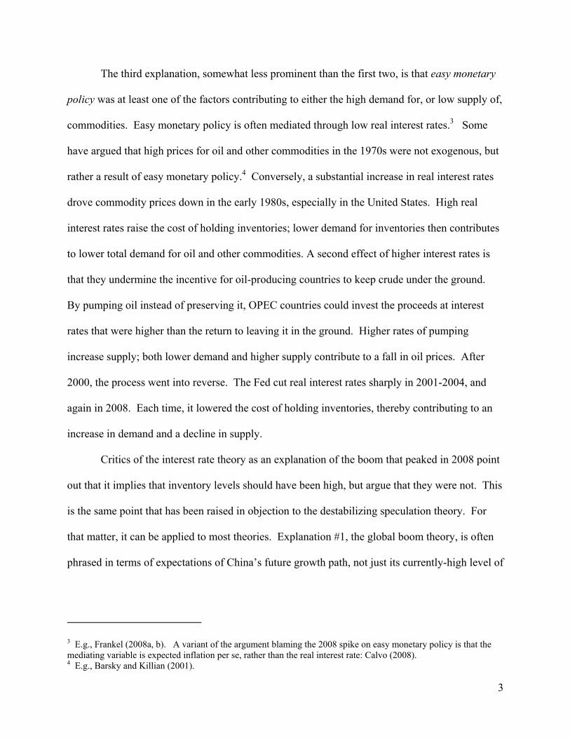
The third explanation, somewhat less prominent than the first two, is that easy monetary

policy was at least one of the factors contributing to either the high demand for, or low supply of,

commodities. Easy monetary policy is often mediated through low real interest rates.3 Some

have argued that high prices for oil and other commodities in the 1970s were not exogenous, but

rather a result of easy monetary policy.4 Conversely, a substantial increase in real interest rates

drove commodity prices down in the early 1980s, especially in the United States. High real

interest rates raise the cost of holding inventories; lower demand for inventories then contributes

to lower total demand for oil and other commodities. A second effect of higher interest rates is

that they undermine the incentive for oil-producing countries to keep crude under the ground.

By pumping oil instead of preserving it, OPEC countries could invest the proceeds at interest

rates that were higher than the return to leaving it in the ground. Higher rates of pumping

increase supply; both lower demand and higher supply contribute to a fall in oil prices. After

2000, the process went into reverse. The Fed cut real interest rates sharply in 2001-2004, and

again in 2008. Each time, it lowered the cost of holding inventories, thereby contributing to an

increase in demand and a decline in supply.

Critics of the interest rate theory as an explanation of the boom that peaked in 2008 point

out that it implies that inventory levels should have been high, but argue that they were not. This

is the same point that has been raised in objection to the destabilizing speculation theory. For

that matter, it can be applied to most theories. Explanation #1, the global boom theory, is often

phrased in terms of expectations of China’s future growth path, not just its currently-high level of

                                                            

3 E.g., Frankel (2008a, b). A variant of the argument blaming the 2008 spike on easy monetary policy is that the mediating variable is expected inflation per se, rather than the real interest rate: Calvo (2008). 4 E.g., Barsky and Killian (2001).

  4

income; but this factor, too, if operating in the market place, should in theory work to raise

demand for inventories.5

How might high demand for commodities be reconciled with low observed inventories?

One possibility is that researchers are looking at the wrong inventory data. Standard data

inevitably exclude various components of inventories, such as those held by users or those in

faraway countries. They typically exclude deposits, crops, forests, or herds that lie in or on the

ground. In other words, what is measured in inventory data is small compared to reserves. The

decision by producers whether to pump oil today or to leave it underground for the future is more

important than the decisions of oil companies or downstream users whether to hold higher or

lower inventories. And the lower real interest rates of 2001-2005 and 2008 clearly reduced the

incentive for oil producers to pump oil, relative to what it would otherwise be.6 We classify low

extraction rates as low supply and high inventories as high demand; but either way the result is

upward pressure on prices.

In 2008, enthusiasm for explanations #2 and #3, the speculation and interest rate theories,

increased, at the expense of theory #1, the global boom. Previously, rising demand from the

global expansion, especially the boom in China, had seemed the obvious explanation for rising

commodity prices. But the sub-prime mortgage crisis hit the United States around August 2007.

Virtually every month thereafter, forecasts of growth were downgraded, not just for the United

States but for the rest of the world as well, including China.7 Meanwhile commodity prices, far

from declining as one might expect from the global demand hypothesis, climbed at an

                                                            

5 We are indebted to Larry Summers for this point. 6 The King of Saudi Arabia said at this time that his country might as well leave the reserves in the ground for its grandchildren. 7 E.g., World Economic Outlook, International Monetary Fund, October 2007, April 2008, and October 2008. Also OECD and World Bank.

  5

accelerated rate. For the year following August 2007, at least, the global boom theory was

clearly irrelevant. That left explanations #2 and #3.

In both cases – increased demand arising from either low interest rates or expectations of

capital gains -- detractors pointed out that the explanations implied that inventory holdings

should be high and continued to argue that this was not the case.8 To repeat a counterargument,

especially in the case of oil, what is measured in inventory data is small compared to reserves

under the ground. The decision by producers whether to pump oil today or to leave it

underground for the future is more important than the decisions of oil companies or downstream

users whether to hold higher or lower inventories.

The paper presents a theoretical model of the determination of prices for storable

commodities that gives full expression to such macroeconomic factors as economic activity and

real interest rates. However, we do not ignore other fundamentals relevant for commodity price

determination. To the contrary, our model includes a number of microeconomic factors

including (but not limited to) inventories. We then estimate the equation using both

macroeconomic and commodity-specific microeconomic determinants of commodity prices.

2. A Theory of Commodity Price Determination

Most agricultural and mineral products differ from other goods and services in that they

are both storable and relatively homogeneous. As a result, they are hybrids of assets – where

price is determined by supply of and demand for stocks – and goods, for which flow supply and

flow demand matter.9

                                                            

8 See among others, Krugman, 2008, and Kohn, 2008. 9 E.g., Frankel (1984), Calvo (2008).

  6

The elements of an appropriate model have long been known.10 The monetary aspect of

the theory can be reduced to its simplest algebraic essence as a relationship between the real

interest rate and the spot price of a commodity relative to its expected long-run equilibrium price.

This relationship can be derived from two simple assumptions. The first governs expectations.

Let:

s ≡ the natural logarithm of the spot price,

s ≡ its long run equilibrium,

p ≡ the (log of the) economy-wide price index,

q ≡ s-p, the (log) real price of the commodity, and

q ≡ the long run (log) equilibrium real price of the commodity.

Market participants who observe the real price of the commodity today lying either above or

below its perceived long-run value, expect it to regress back to equilibrium in the future over

time, at an annual rate that is proportionate to the gap:

E [ Δ (s – p ) ] ≡ E[ Δq] = - θ (q- q ) (1)

or E (Δs) = - θ (q- q ) + E(Δp). (2)

Following the classic Dornbusch (1976) overshooting paper, which developed the model for the

case of exchange rates, we begin by simply asserting the reasonableness of the form of

expectations in these equations. It seems reasonable to expect a tendency for prices to regress

                                                            

10 E.g., Frankel (1986, 2008), among others.

  7

back toward long run equilibrium. But, as in that paper, it can be shown that regressive

expectations are also rational expectations, under certain assumptions regarding the stickiness of

prices of other goods (manufactures and services) and a certain restriction on the parameter value

θ.11

One alternative that we considered below is that expectations also have an extrapolative

component to them. We model this as:

E (Δs) = - θ (q- q ) + E(Δp) + δ (Δs -1 ) (2’)

The next equation concerns the decision whether to hold the commodity for another

period – leaving it in the ground, on the trees, or in inventory – or to sell it at today’s price and

deposit the proceeds to earn interest. The expected rate of return to these two alternatives must

be the same:

E Δs + c = i, where c ≡ cy – sc – rp . (3)

where:

cy ≡ convenience yield from holding the stock (e.g., the insurance value of having an assured

supply of some critical input in the event of a disruption, or in the case of gold the psychic

pleasure component of holding it),

sc ≡ storage costs (e.g., feed lot rates for cattle, silo rents and spoilage rates for grains, , rental

rate on oil tanks or oil tankers, costs of security to prevent plundering by others, etc.),

12  

                                                            

11 Frankel (1986). 12 Fama and French (1987) and Bopp and Lady (1991) emphasize storage costs.

  8

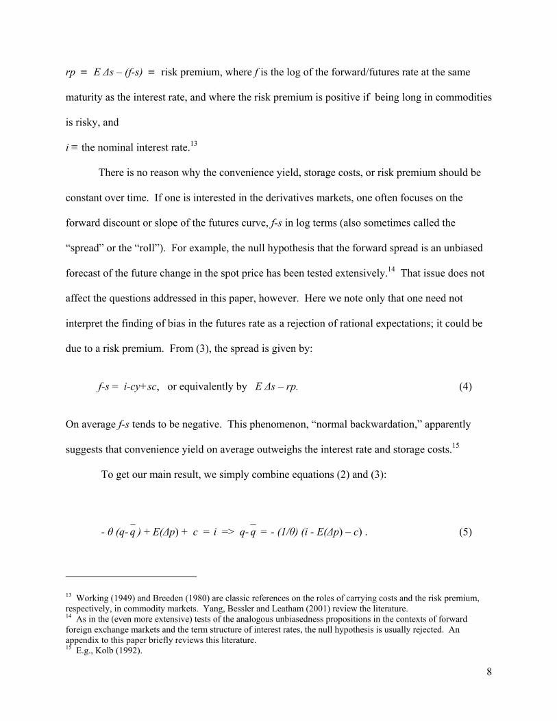
rp ≡ E Δs – (f-s) ≡ risk premium, where f is the log of the forward/futures rate at the same

maturity as the interest rate, and where the risk premium is positive if being long in commodities

is risky, and

i ≡ the nominal interest rate.13

There is no reason why the convenience yield, storage costs, or risk premium should be

constant over time. If one is interested in the derivatives markets, one often focuses on the

forward discount or slope of the futures curve, f-s in log terms (also sometimes called the

“spread” or the “roll”). For example, the null hypothesis that the forward spread is an unbiased

forecast of the future change in the spot price has been tested extensively.14 That issue does not

affect the questions addressed in this paper, however. Here we note only that one need not

interpret the finding of bias in the futures rate as a rejection of rational expectations; it could be

due to a risk premium. From (3), the spread is given by:

f-s = i-cy+sc, or equivalently by E Δs – rp. (4)

On average f-s tends to be negative. This phenomenon, “normal backwardation,” apparently

suggests that convenience yield on average outweighs the interest rate and storage costs.15

To get our main result, we simply combine equations (2) and (3):

- θ (q- q ) + E(Δp) + c = i => q- q = - (1/θ) (i - E(Δp) – c) . (5)

                                                            

13 Working (1949) and Breeden (1980) are classic references on the roles of carrying costs and the risk premium, respectively, in commodity markets. Yang, Bessler and Leatham (2001) review the literature. 14 As in the (even more extensive) tests of the analogous unbiasedness propositions in the contexts of forward foreign exchange markets and the term structure of interest rates, the null hypothesis is usually rejected. An appendix to this paper briefly reviews this literature. 15 E.g., Kolb (1992).

  9

Equation (5) says that the real price of the commodity, measured relative to its long-run

equilibrium, is inversely proportional to the real interest rate (measured relative to a constant

term). When the real interest rate is high, as in the 1980s, money flows out of commodities.

Only when the prices of commodities are perceived to lie sufficiently below their future

equilibria, generating expectations of future price increases, will the quasi-arbitrage condition be

met. Conversely, when the real interest rate is low, as in 2001-05 and 2008-09, money flows

into commodities. This is the same phenomenon that also sends money flowing to foreign

currencies (“the carry trade”), emerging markets, and other securities. Only when the prices of

commodities (or the other alternative assets) are perceived to lie sufficiently above their future

equilibria, generating expectations of future price decreases, will the speculative condition be

met.

Under the alternative specification that leaves a possible role for bandwagons, we

combine equations (2’) and (3) to get:

q- q = - (1/θ) (i - E(Δp) – c) + (δ /θ) (Δs -1 ). (5’)

As noted, there is no reason for the “constant term” in equation (5) to be constant.

Substituting from (3) into (5),

c ≡ cy – sc – rp =>

q- q = - (1/θ) [i - E(Δp) – cy + sc + rp ]

q= q - (1/θ) [i-E(Δp)] + (1/θ) cy - (1/θ) sc - (1/θ) rp . (6)

Thus, even if we continue to take the long-run equilibrium q as given, there are other variables

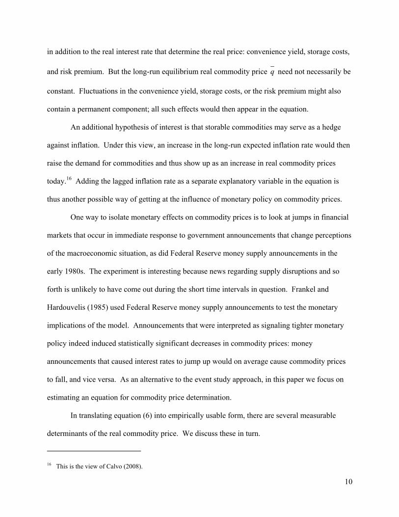
  10

in addition to the real interest rate that determine the real price: convenience yield, storage costs,

and risk premium. But the long-run equilibrium real commodity price q need not necessarily be

constant. Fluctuations in the convenience yield, storage costs, or the risk premium might also

contain a permanent component; all such effects would then appear in the equation.

An additional hypothesis of interest is that storable commodities may serve as a hedge

against inflation. Under this view, an increase in the long-run expected inflation rate would then

raise the demand for commodities and thus show up as an increase in real commodity prices

today.16 Adding the lagged inflation rate as a separate explanatory variable in the equation is

thus another possible way of getting at the influence of monetary policy on commodity prices.

One way to isolate monetary effects on commodity prices is to look at jumps in financial

markets that occur in immediate response to government announcements that change perceptions

of the macroeconomic situation, as did Federal Reserve money supply announcements in the

early 1980s. The experiment is interesting because news regarding supply disruptions and so

forth is unlikely to have come out during the short time intervals in question. Frankel and

Hardouvelis (1985) used Federal Reserve money supply announcements to test the monetary

implications of the model. Announcements that were interpreted as signaling tighter monetary

policy indeed induced statistically significant decreases in commodity prices: money

announcements that caused interest rates to jump up would on average cause commodity prices

to fall, and vice versa. As an alternative to the event study approach, in this paper we focus on

estimating an equation for commodity price determination.

In translating equation (6) into empirically usable form, there are several measurable

determinants of the real commodity price. We discuss these in turn.

                                                            

16 This is the view of Calvo (2008).

  11

Inventories. Storage costs rise with the extent to which inventory holdings strain existing

storage capacity: sc = Φ (INVENTORIES). If the level of inventories is observed to be at the high end

historically, then storage costs must be high (absent any large recent increase in storage

capacity), which has a negative effect on commodity prices.17 Substituting into equation (6),

q= q - (1/θ) [i-E(Δp)] + (1/θ) cy - (1/θ) Φ (INVENTORIES) - (1/θ) rp . (7)

There is no reason to think that the relationship Φ is necessarily linear. We assume

linearity in our estimation for simplicity, but allowing for non-linearity is a desirable extension

of the analysis. Under the logic that inventories are bounded below by zero and above by some

absolutely peak storage capacity, a logistic function might be appropriate.

If one wished to estimate an equation for the determination of inventory holdings, once

could use:

INVENTORIES = Φ-1 ( sc ) = Φ-1 (cy - i – (s-f) ) (8)

We see that low interest rates should predict not only high commodity prices but also high

inventory holdings.

Economic Activity (denoted Y) is a determinant of the convenience yield cy, since it

drives the transactions demand for inventories. Higher economic activity should have a positive

effect on the demand for inventory holdings and thus on prices; we usually proxy this with GDP.

Let us designate the relationship γ (Y). Again, the assumption of linearity is arbitrary.

                                                            

17 Ye et al (2002, 2005, 2006) emphasize the role of inventories in forecasting oil prices.

  12

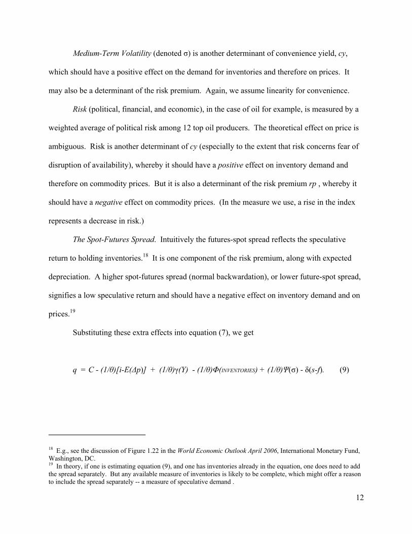
Medium-Term Volatility (denoted σ) is another determinant of convenience yield, cy,

which should have a positive effect on the demand for inventories and therefore on prices. It

may also be a determinant of the risk premium. Again, we assume linearity for convenience.

Risk (political, financial, and economic), in the case of oil for example, is measured by a

weighted average of political risk among 12 top oil producers. The theoretical effect on price is

ambiguous. Risk is another determinant of cy (especially to the extent that risk concerns fear of

disruption of availability), whereby it should have a positive effect on inventory demand and

therefore on commodity prices. But it is also a determinant of the risk premium rp , whereby it

should have a negative effect on commodity prices. (In the measure we use, a rise in the index

represents a decrease in risk.)

The Spot-Futures Spread. Intuitively the futures-spot spread reflects the speculative

return to holding inventories.18 It is one component of the risk premium, along with expected

depreciation. A higher spot-futures spread (normal backwardation), or lower future-spot spread,

signifies a low speculative return and should have a negative effect on inventory demand and on

prices.19

Substituting these extra effects into equation (7), we get

q = C - (1/θ)[i-E(Δp)] + (1/θ)γ(Y) - (1/θ)Φ(INVENTORIES) + (1/θ)Ψ(σ) - δ(s-f). (9)

                                                            

18 E.g., see the discussion of Figure 1.22 in the World Economic Outlook April 2006, International Monetary Fund, Washington, DC. 19 In theory, if one is estimating equation (9), and one has inventories already in the equation, one does need to add the spread separately. But any available measure of inventories is likely to be complete, which might offer a reason to include the spread separately -- a measure of speculative demand .

  13

Finally, to allow for the possibility of bandwagons and bubbles, and a separate effect of inflation

on commodity prices, we use the alternative expectations equation (5’) in place of (5). Equation

(9) then becomes:

q = C - (1/θ)[i-E(Δp)] + (1/θ)γY - (Φ/θ) (INVENTORIES)

+ (Ψ/θ) σ - δ(s-f) + λ E(Δp) + (δ /θ)(Δs-1). (9')

It is this equation – augmented by a hopefully well-behaved residual term – which we wish to

investigate.

Each of the variables on the right-hand side of equation (9) could easily be considered

endogenous. This must be considered a limitation of our analysis. In future extensions, we

would like to consider estimating three simultaneous equations: one for expectations formation,

one for the inventory arbitrage condition, and one for commodity price determination. However,

we are short of plausibly exogenous variables with which to identify such equations. From the

viewpoint of an individual commodity though, aggregate variables such as the real interest rate

and GDP can reasonably be considered exogenous.20

3. The Data Set

We begin with a preliminary examination of the data set, starting with the

macroeconomic determinants of commodity prices.

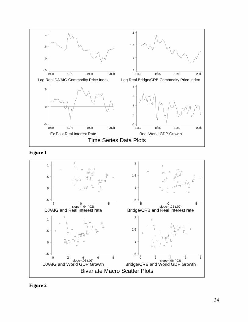
Figure 1 contains time-series plots for four variables of interest. The top pair portray the

natural logarithms of two popular commodity price indices (the Dow-Jones/AIG and the                                                             

20 Also inventories could perhaps be considered pre-determined in higher frequency data, since it takes time to make big additions to or subtractions from inventories. But in this paper we use annual data.

  14

Bridge/CRB indices). Both series have been deflated by the American GDP chain price index to

make them real. Below them are portrayed: the annualized realized American real interest rate

(defined as the 3-month Treasury-bill rate at auction less the percentage change in the American

chain price index) and the growth rate of real World GDP (taken from the World Bank’s World

Development Indicators). All data are annual and span 1960 through 2008.

We follow the literature and measure commodity prices in American dollar terms and use

real American interest rates. We think this is a reasonable way to proceed. If commodity

markets are nationally segmented, by trade barriers and transport costs, then local commodity

prices are determined by domestic real interest rates, domestic economic activity and so on. It is

reasonable to assume, however, that world commodity markets are closer to integrated than they

are to being segmented. Indeed, many assume that the law of one price holds closely for

commodities.21 In this case, the nominal price of wheat in Australian dollars is the nominal price

in terms of US dollars multiplied by the nominal exchange rate.22 Equivalently, the real price of

wheat in Australia is the real price in the US times the real exchange rate.23

Figure 1 contains few surprises. The sharp run-up in real commodity prices in the

early/mid-1970s is clearly visible as is the most recent rise. Real interest rates were low during

both periods of time, and high during the early 1980s, as expected. Global business cycle

movements are also clearly present in the data.

                                                            

21 For example, Phillips and Pippenger (2005) and Protopapdakis and Stoll (1983, 1986).  22 For example, Mundell (2002). 23 An application of the Dornbusch overshooting model can give us the prediction that the real exchange rate is proportionate to the real interest differential. It thus turns out that the real commodity price in local currency can be determined by the US real interest rate (and other determinants of the real US price) together with the differential in real interest rates between the domestic country and the US. Equations along these lines are estimated in Frankel (2008; Table 7.3) for real commodity price indices in eight floating-rate countries: Australia, Brazil, Canada, Chile, Mexico, New Zealand, Switzerland, and the United Kingdom. In almost every case, both the US real interest rate and the local-US real interest differential are found to have significant negative effects on local real commodity prices, just as hypothesized.

  15

Figure 2 provides simple scatter-plots of both real commodity price series against the two

key macroeconomic phenomena. The bivariate relationships seem weak; real commodity prices

are slightly negatively linked to real interest rates and positively to world growth. We interpret

this to mean that there is plenty of room for microeconomic determinants of real commodity

prices, above and beyond macroeconomic phenomena.24 Accordingly, we now turn from

aggregate commodity price indices and explanatory variables to commodity-specific data.

We have collected data on prices and microeconomic fundamentals for twelve

commodities of interest.25 Seven are agricultural, including a number of crops (corn, cotton,

oats, soybeans, and wheat), as well as two livestock variables (live cattle and hogs). We also

have petroleum and four non-ferrous metals (copper, gold, platinum, and silver). We chose the

span, frequency, and choice of commodities so as to maximize data availability. The series are

annual, and typically run from some time after the early 1960s through 2008.26

Figure 3 is a series of time-series plots of the natural logarithm of commodity prices, each

deflated by the American GDP chain price index. The log of the real price shows the boom of

the 1970s in most commodities and the second boom that culminated in 2008 – especially in the

minerals: copper, gold, oil and platinum.

Figures 4 through 7 portray the commodity-specific fundamentals used as explanatory

variables when we estimate equation (9). We measure volatility as the standard deviation of the

spot price over the last year.27 According to our inventory data, some commodities show

inventories that in 2008 were fairly high historically after all: corn, cotton, hogs, oil, and

                                                            

24 Frankel (2008) finds stronger evidence, especially for the relationship of commodity price indices and real interest rates. 25 We often are forced to drop gold, since we have no data on gold inventories. 26 Further details concerning the series, and the data set itself, are available on the internet. 27 Alternative measurements are possible; in the future, we hope to use the implicit forward-looking expected volatility that can be extracted from options prices.

  16

soybeans.28 The future-spot spread alternates frequently between normal backwardation and

contango. As one can see, the political risk variables are relatively limited in availability;

accordingly, we do not include them in our basic estimating equation, but use them for

sensitivity analysis. Imaginative eyeballing can convince one that oil producers show high risk

around the time of the 1973 Arab oil embargo and the aftermath of the 2001 World Trade Center

attack. Further details on the commodity-specific series, and the data themselves, are available

on the internet.

Finally, our preferred measure of real activity is plotted in Figure 8; (log) Real Gross

World Product. This has the advantage of including developing countries including China and

India. Of course all economic activity variables have positive trends. One must detrend them to

be useful measures of the business cycle; we include a linear trend term in all our empirical

work. (Another way to think of the trend term is as capturing the trend in supply capacity or

storage capacity.) The growth rate of world GDP is also shown in Figure 8, as is world output

detrended via the HP-filter. Finally, we also experiment with the output gap, which is available

only for the OECD collectively, and only since 1970. In any of the measures of real economic

activity one can see the recessions of 1975, 1982, 1991, 2001, and 2008.29

4. Estimation of Commodity Price Determination Equation

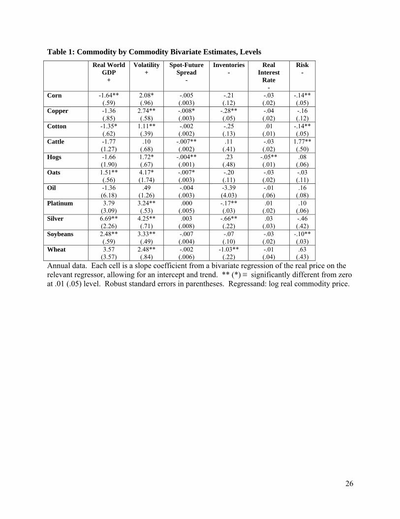
As a warm-up, Table 1 reports results of bivariate regressions; we show coefficients

along with robust standard errors. The correlation with real economic activity is reported in the

first column. Surprisingly, real prices are not significantly correlated with global output for most

                                                            

28 We use world inventories insofar as possible, but substitute American inventories when this is missing (specifically, in the cases of copper, live cattle and hogs, oats, platinum and silver). We do not have any gold inventory data at all. 29 In the past, we have also used American GDP, G-7 GDP, and industrial production (for the US as well as for advanced countries in the aggregate); the latter has the advantage of being available monthly.

  17

commodities; the exceptions are oats, silver and soybeans.30 Volatility shows a positive bivariate

correlation with all prices, significantly so for nine out of eleven commodities. The correlations

with the spot-futures spread and inventories are also almost always of the hypothesized sign

(negative), and significant for a number of commodities. The real interest rate, too, shows the

hypothesized negative correlation for eight out of eleven commodity prices, but is significantly

different from zero for only one commodity, hogs. Political risk is significantly different from

zero in just four cases: higher political risk appears to raise demand for corn, cotton and

soybeans (a negative coefficient in the last column of Table 1), but to lower it for cattle. As with

volatility, the theoretical prediction is ambiguous: the positive correlation is consistent with the

convenience yield effect, and the negative correlation with the risk premium effect.31

The theory made it clear that prices depend on a variety of independent factors

simultaneously, so these bivariate correlations may tell us little. Accordingly, Table 2a presents

the multivariate estimation of equation (9).32 World output now shows the hypothesized positive

coefficient in nine out of eleven commodities, and is statistically significant in four of them:

corn, cattle, oats and soybeans. That is, economic activity significantly raises demand for these

commodities. The coefficient on volatility is statistically greater than zero for five commodities:

copper, platinum, silver, soybeans and wheat. Evidently, at least for these five goods, volatility

raises the demand to hold inventories, via the convenience yield. The spread and inventories are

                                                            

30 When we substitute G-7 real GDP, the three commodity prices that showed significant correlations -- not reported here -- were: corn, cotton and soybeans. We view global output as a better measure than G-7 GDP or industrial production, because it is more comprehensive. 31 The results were a bit better when the same tests were run in terms of first differences (on data through 2007, reported not here [but rather in Table 1b of the Muenster draft]). Correlation of price changes with G-7 GDP changes was always positive, though again significant only for corn, cotton and soybeans. Correlations with volatility, the spread, and inventories each show up as significant in five or six commodities out of 11. 32 We exclude the political risk measure. It gives generally unclear results, perhaps in part because its coverage is incomplete, perhaps because of the possible theoretical ambiguity mentioned earlier. Volatility seems to be better at capturing risk. A useful extension would be to use implicit volatility from options prices, which might combine the virtues of both the volatility and political risk variables.

  18

usually of the hypothesized negative sign (intuitively, backwardation signals expected future

reduction in commodity values while high inventory levels imply that storage costs are high).

However, the effects are significant only for a few commodities. The coefficient on the real

interest rate is of the hypothesized negative sign in seven of the eleven commodities, but

significantly so only for two: cattle and hogs. Overall, the macro variables work best for cattle.

They work less well for the metals than for agricultural commodities, which would be surprising

except that the same pattern appeared in Frankel (2008).

When the regressions are run in first differences, in Table 2b, the output coefficient is

now always of the hypothesized positive sign. But the coefficient is smaller in magnitude, and

less often significant. Volatility is still significantly positive in five commodities, the spot-

futures spread significantly negative in four, and inventories significantly negative for two. Any

effect of the real interest rate has vanished.

Analyzing commodities one at a time manifestly does not generally produce strong

evidence. This may not be surprising. For one thing, because we are working with annual data

here, each regression has relatively few observations. For another thing, we know that we have

not captured idiosyncratic forces such as the weather events that lead to bad harvests in some

regions or the political unrest that closes mines in other parts of the world. We hope to learn

more when we combine data from different commodities together.

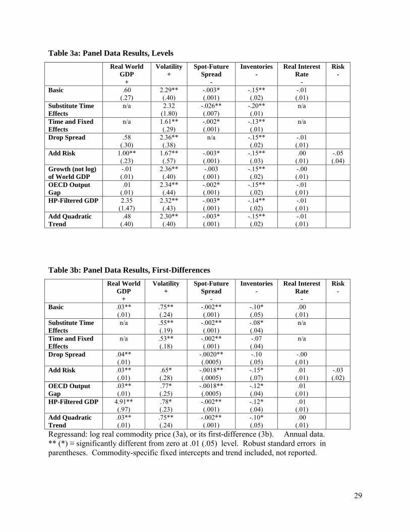
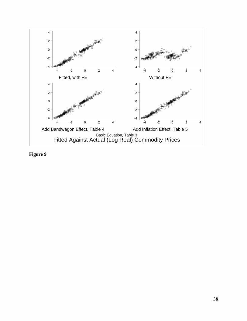
Tables 3a and 3b are probably our most important findings. They pool data from

different commodities together into one large panel data set.33 In the panel setting, with all the

data brought to bear, the theory is supported more strongly. The basic equation, with fixed

effects for each commodity, is portrayed in the first row. The coefficients on world output and                                                             

33 Unless otherwise noted, in our panel estimation we always include a common trend and commodity-specific intercepts; we simply do not report those coefficients.

  19

volatility have the expected positive effects; the latter is significantly different from zero at the

1% level, while the former misses significance by a whisker (the significance level is 5.3%).

The coefficients on the spread and inventories are significantly different from zero with the

hypothesized negative effects; and the coefficient on the real interest rate, though not significant,

is of the hypothesized negative sign. Our basic equation also fits the data reasonably; the within-

commodity R2=.58, though the between-commodity R2 is a much lower .15 (as expected). The

fitted values are graphed against the actual (log real) commodity prices in the top-left graph of

Figure 9. (The graph immediately to the right shows the results when the fixed effects are

removed from the fitted values.)

Table 3a also reports a variety of extensions and sensitivity tests in the lower rows. The

third row substitutes year-specific fixed effects in place of the commodity-specific ones; the next

row adds year-specific to commodity-specific fixed effects. The two macroeconomic variables,

world output and the real interest rate, necessarily drop out in the presence of these time effects;

by definition they do not vary within a cross-section of commodities. But it is reassuring that the

three remaining (microeconomic) variables – volatility, the spread, and inventories – retain their

significant effects. The next row drops the spot-forward spread from the specification on the

grounds that its role may already be played by inventories (see equation (7)). The effects of

inventories and the other variables remain essentially unchanged. Next, we add the political risk

variable back in. It is statistically insignificant, but in its presence the world output variable

becomes more significant than ever. We then try four alternative measures of global economic

activity in place of the log of real world GDP: 1) the growth rate of world output, 2) the OECD

output gap; 3) Hodrick-Prescott filtered GDP, and 4) log real world GDP with a quadratic trend.

  20

None works as well as Gross World Output, but the microeconomic effects are essentially

unchanged.

Table 3b repeats the exercise of Table 3a, but using first-differences rather than (log-)

levels, with similar results. In particular, the signs for the microeconomic determinants are

almost always as hypothesized, as is the effect of economic activity. Most of the coefficients are

also significantly different from zero, though the effect of activity on commodity prices is much

smaller than in Table 3a. The estimated effects of real interest rates are often positive and never

significant.

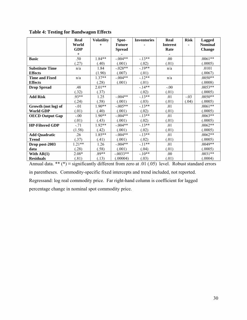
Table 4 retains the panel estimation technique of Tables 3a and 3b, but reports the

outcome of adding the rate of change of the spot commodity price over the preceding year to the

standard list of determinants. The rationale is to test the theory of destabilizing speculation by

looking for evidence of bandwagon expectations, as in equation (9’). The lagged change in the

spot price is indeed highly significant statistically, even if time effects are added, data after 2003

are dropped, or auto-correlated residuals are included in the estimation. It is significant

regardless whether the spread or political risk variables are included or not, and regardless of the

measure of economic activity. Evidently, alongside the regular mechanism of regressive

expectations that is built into the model (a form of stabilizing expectations), there is at the same

time a mechanism of extrapolative expectations (which is capable of producing self-confirming

bubble movements).

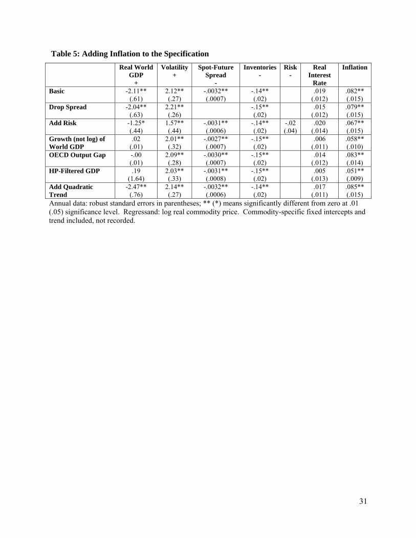
Table 5 reports the result of adding a separate coefficient for the American inflation rate,

above and beyond the real interest rate (and the other standard commodity price determinants).

Thus there are two separate measures of the monetary policy stance. Recall that the

hypothesized role of the real interest rate is to pull the current real commodity price q away from

  21

its long run equilibrium q , while the role of the expected inflation rate is to raise the long run

equilibrium price q to the extent that commodities are considered useful as a hedge against

inflation. In our default specification, and under almost all of the variations, the coefficient on

inflation is greater than zero and highly significant. The result suggests that commodities are

indeed valued as a hedge against inflation. The positive effect of inflation offers a third purely

macroeconomic explanation for commodity price movements (alongside real interest rates,

which don’t work very well in our results, and growth which does). 34,35

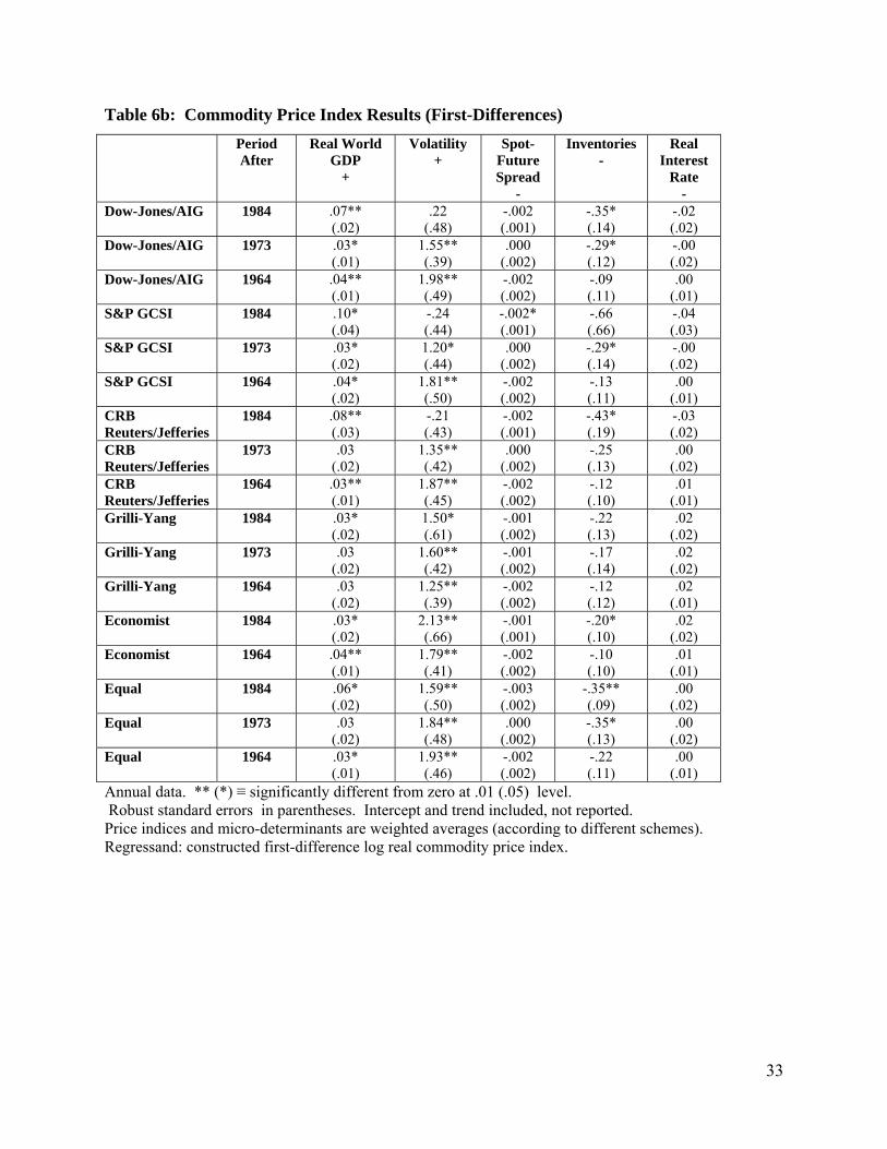
Tables 6a and 6b report the results for a variety of aggregate commodity price indices

that we have created. Prices and each of the relevant determinant variables has been aggregated

up using commodity-specific data and (time-invariant) weights from a particular index. We use

weights from five popular indices (Dow Jones/AIG; S&P/GCSI; CRB Reuters/Jeffries; Grilli-

Yang; and Economist), and also create an equally-weighted index. Since these rely on a number

of commodities for which we do not have data, our constructed indices are by no means equal to

the original indices (such as those portrayed in Figures 1 and 2). Further, the span of data

available over time varies by commodity. Accordingly, we create three different indices for each

weighting scheme; the narrowest (in that it relies on the fewest commodities) stretches back to

1964, while broader indices are available for shorter spans of time (we create indices that begin

in 1973 and 1984). We use the same weights for prices and their fundamental determinants. The

benefit from this aggregation is that some of the idiosyncratic influences that are particular to the

individual commodities, such as weather, may wash out when we look at aggregate indices. The

cost is that we are left with many fewer observations.                                                             

34 E.g., Calvo (2008). 35 Adding either a bandwagon or inflationary effect improves the fit of our equation: the within R2 rises from .58 to .66 in both cases. Fitted values for both perturbations are graphed against actual prices in the bottom graphs of Figure 9.

  22

In the first column of Table 6a – which reports results in levels – the real GDP output

coefficient always has the hypothesized positive sign. However, it is only significant in Table

6b, where the estimation is in terms of first differences. The volatility coefficient is almost

always statistically greater than zero in both Tables 6a and 6b. The coefficient on the spot-

futures spread is almost always negative, but not usually significantly different from zero. The

inventory coefficient too is almost always negative, and sometimes significant. The real interest

rate is never significant, though the sign is generally negative (and always negative in Table 6a).

The lack of statistical significance probably arises because now that we are dealing with short

time series of aggregate indices, so that the number of observations is smaller than in the panel

analysis; this is especially true in the cases where we start the sample later.

Although we have already reported results of regressions run in both levels and first

differences, a complete analysis requires that we examine the stationarity or nonstationarity of

the series more formally. Tables in the second appendix tabulate Phillips-Perron tests for unit

roots in our individual variables; the aggregate series are handled in Appendix Table 1a, while

the commodity-specific series are done in Appendix Table 1b. Appendix Table 1c is the

analogue that tests for common panel unit roots. The tests often fail to reject unit roots (though

not for the spread and volatility). One school of thought would doubt on a priori grounds that

variables such as the real interest rate could truly follow a random walk. The other school of

thought says that one must go wherever the data instruct. Here we pursue the implication of unit

roots to be safe, as a robustness check if nothing else. However, we are reluctant to over-

interpret our results, especially given the short number of time-series observations.36

                                                            

36 Studies of the time series properties of real commodity prices can find a negative trend, positive trend, random walk, or mean reversion, depending on the sample period available when the authors do their study. Examples include Cuddington and Urzua (1989) and Reinhart and Wickham (1994).

  23

Appendix Tables 2a – 2c report related tests of cointegration. We generally find

cointegration in commodity-specific models, but have weaker results in our panel cointegration

result. It is not clear to us whether this is the result of low power, the absence of fixed effects, or

some other mis-specification. Still, appendix Table 3 reports results from commodity-specific

vector error correction models. As in some of the previous tests, the three variables that are most

consistently significant and of the hypothesized sign are the spread, the volatility, and

inventories. We view this as reassuring corroboration of the panel estimation we have already

documented.

4. Summary and Conclusion

This paper has presented a model that can accommodate each of the prominent

explanations that were given for the run-up in prices of most agricultural and mineral

commodities that culminated in the 2008 spike: global economic activity, easy monetary policy,

and destabilizing speculation. Our model includes both macroeconomic and microeconomic

determinants of real commodity prices, both theoretically and empirically.

The theoretical model is built around the “arbitrage” decision faced by any firm holding

inventories. This is the tradeoff between the carrying cost of the inventory on the one hand (the

interest rate plus the cost of storage) versus the convenience yield and forward-spot spread (or, if

unhedged, the expected capital gains adjusted for the risk premium), on the other hand. A

second equation completes the picture; the real commodity price is expected to regress gradually

in the future back to its long run equilibrium (at least absent bandwagon expectations). The

reduced form equation then gives the real commodity price as a function of the real interest rate,

storage costs, convenience yield, and risk premium. The level of inventories is a ready stand-in

for storage costs. The empirical significance of the inventory variable suggests that the data and

  24

relationship are meaningful, notwithstanding fears that the available measures of inventories

were incomplete.37 Global growth is an important determinant of convenience yield. Measures

of political risk and price uncertainty are other potentially important determinants of both

convenience yield and the risk premium.

Our strongest results come when we bring together as much data as possible, in the panel

estimates of Tables 3, 4 and 5. Our annual empirical results show support for the influence of

economic activity, inventories, uncertainty, the spread and recent spot price changes. The

significance of the inventories variable supports the legitimacy of arguments by others who have

used observed inventory levels to reason about the roles of speculation or interest rates.

Unfortunately, there was little support in these new annual results for the hypothesis that easy

monetary policy and low real interest rates are an important source of upward pressure on real

commodity prices, beyond any effect they might have via real economic activity and inflation

(This result differs from more positive results of previous papers.) We also find evidence that

commodity prices are driven in part by bandwagon expectations and by inflation per se.

A number of possible extensions remain for future research. These include: 1) estimation

at monthly or quarterly frequency (the big problem here is likely to be data availability,

especially for any reasonably long span of time) ; 2) testing for nonlinearity in the effects of

growth, uncertainty and (especially) inventories; 3) using implicit volatility inferred from

commodity options prices as the measure of uncertainty; 4) using survey data to measure

commodity price expectations explicitly; and 5) simultaneous estimation of the three equations:

expectations formation (regressive versus bandwagon), the inventory arbitrage condition, and the

equation for determination of the real commodity price. The future agenda remains large.                                                             

37 We are implicitly considering inventories relative to full capacity, but explicit adjustment would improve the measurement, if the appropriate data on storage capacity could be found.

  25

What caused the run-up in commodities prices in the 2000s? One theory is that they were

caused by recent rapid global growth – as in the 1970s – aided now by China and India.

Presumably, then the abrupt decline in the latter part of 2008, and even the partial recovery in the

spring of 2009, could be explained by the rapidly evolving prospects for the real economy. But

this story is still not able to explain the acceleration of commodity prices between the summer of

2007 and the peak in the fall of 2008, a time when growth prospects were already being

downgraded in response to the US sub-prime mortgage crisis. Of the two candidate theories to

explain that interval – low real interest rates and a speculative bubble – there is more support for

the latter in this paper, in the form of bandwagon expectations. But a more definitive judgment

on both may have to await higher-frequency data.

  26

Table 1: Commodity by Commodity Bivariate Estimates, Levels Real World

GDP +

Volatility +

Spot-Future Spread

-

Inventories-

Real Interest

Rate -

Risk -

Corn -1.64** (.59)

2.08* (.96)

-.005 (.003)

-.21 (.12)

-.03 (.02)

-.14** (.05)

Copper -1.36 (.85)

2.74** (.58)

-.008* (.003)

-.28** (.05)

-.04 (.02)

-.16 (.12)

Cotton -1.35* (.62)

1.11** (.39)

-.002 (.002)

-.25 (.13)

.01 (.01)

-.14** (.05)

Cattle -1.77 (1.27)

.10 (.68)

-.007** (.002)

.11 (.41)

-.03 (.02)

1.77** (.50)

Hogs -1.66 (1.90)

1.72* (.67)

-.004** (.001)

.23 (.48)

-.05** (.01)

.08 (.06)

Oats 1.51** (.56)

4.17* (1.74)

-.007* (.003)

-.20 (.11)

-.03 (.02)

-.03 (.11)

Oil -1.36 (6.18)

.49 (1.26)

-.004 (.003)

-3.39 (4.03)

-.01 (.06)

.16 (.08)

Platinum 3.79 (3.09)

3.24** (.53)

.000 (.005)

-.17** (.03)

.01 (.02)

.10 (.06)

Silver 6.69** (2.26)

4.25** (.71)

.003 (.008)

-.66** (.22)

.03 (.03)

-.46 (.42)

Soybeans 2.48** (.59)

3.33** (.49)

-.007 (.004)

-.07 (.10)

-.03 (.02)

-.10** (.03)

Wheat 3.57 (3.57)

2.48** (.84)

-.002 (.006)

-1.03** (.22)

-.01 (.04)

.63 (.43)

Annual data. Each cell is a slope coefficient from a bivariate regression of the real price on the relevant regressor, allowing for an intercept and trend. ** (*) ≡ significantly different from zero at .01 (.05) level. Robust standard errors in parentheses. Regressand: log real commodity price.

  27

Table 2a: Multivariate Regressions, Commodity by Commodity Estimates, Levels Real

World GDP +

Volatility +

Spot-Future Spread

-

Inventories -

Real Interest Rate

- Corn 1.53*

(.69) 1.52 (.89)

-.003 (.003)

-.18 (.17)

-.01 (.02)

Copper .03 (.68)

1.92** (.54)

-.005 (.003)

-.21** (.06_

-.03 (.01)

Cotton .66 (.85)

1.07 (.57)

-.002 (.002)

-.12 (.14)

.01 (.01)

Cattle 7.37** (1.03)

-.65 (.34)

-.007 (.002)

2.37** (.48)

-.06** (.01)

Hogs -.57 (1.64)

.64 (.71)

-.004* (.002)

.18 (.31)

-.03** (.01)

Oats 2.66** (.71)

3.28 (1.69)

-.006** (.002)

-.59** (.11)

-.02 (.01)

Oil .05 (8.60)

.57 (1.69)

-.003 (.003)

-2.52 (5.02)

-.01 (.07)

Platinum 1.22 (2.17)

1.78* (.87)

.002 (.002)

-.21** (.03)

.08** (.01)

Silver 2.69 (2.13)

3.32** (.73)

.003 (.003)

-.37* (.18)

.01 (.03)

Soybeans 1.94** (.70)

2.68** (.55)

-.001 (.002)

-.05 (.07)

-.01 (.01)

Wheat -5.98* (2.79)

1.90** (.47)

.008* (.003)

-1.42** (.27)

.03 (.02)

Annual data. OLS, commodity by commodity (so each row represents a different regression). ** (*) means significantly different from zero at .01 (.05) level. Robust standard errors in parentheses. Intercept and linear time trend included, not recorded. Regressand: log real commodity price.

  28

Table 2b: Commodity by Commodity Multivariate Results, First-Differences Real

World GDP +

Volatility +

Spot-Future Spread

-

Inventories -

Real Interest Rate

- Corn .02

(.02) 1.01 (.53)

-.001 (.001)

-.21 (.12)

-.01 (.02)

Copper .07** (.02)

.44 (.27)

-.002 (.001)

-.08 (.07)

.03 (.02)

Cotton .01 (.02)

1.05** (.37)

-.001 (.001)

-.02 (.13)

.02 (.03)

Cattle .01 (.02)

-.46 (.50)

-.004** (.001)

-1.26 (.96)

-.00 (.01)

Hogs .02 (.03)

-.76 (.85)

-.003** (.001)

-.56 (.50)

-.02 (.02)

Oats .03 (.02)

1.76* (.71)

-.005** (.001)

-.65** (.12)

-.02 (.02)

Oil .10 (.06)

-.34 (.49)

-.003** (.001)

.02 (1.24)

-.04 (.04)

Platinum .03 (.03)

1.28** (.44)

.000 (.001)

-.02 (.07)

.02 (.03)

Silver .01 (.04)

1.98** (.47)

.003 (.003)

-.03 (.10)

.01 (.04)

Soybeans .05** (.02)

1.68** (.37)

-.001 (.001)

.01 (.08)

-.02 (.02)

Wheat .03 (.04)

.90 (.53)

.004 (.002)

-.89** (.23)

-.02 (.04)

Annual data. OLS, commodity by commodity (so each row represents a different regression). ** (*) means significantly different from zero at .01 (.05) level. Robust standard errors in parentheses. Intercept and linear time trend included, not reported. Regressand: first-difference in log real commodity price.

  29

Table 3a: Panel Data Results, Levels Real World

GDP +

Volatility +

Spot-Future Spread

-

Inventories -

Real Interest Rate

-

Risk -

Basic .60 (.27)

2.29** (.40)

-.003* (.001)

-.15** (.02)

-.01 (.01)

Substitute Time Effects

n/a 2.32 (1.80)

-.026** (.007)

-.20** (.01)

n/a

Time and Fixed Effects

n/a 1.61** (.29)

-.002* (.001)

-.13** (.01)

n/a

Drop Spread .58 (.30)

2.36** (.38)

n/a -.15** (.02)

-.01 (.01)

Add Risk 1.00** (.23)

1.67** (.57)

-.003* (.001)

-.15** (.03)

.00 (.01)

-.05 (.04)

Growth (not log) of World GDP

-.01 (.01)

2.36** (.40)

-.003 (.001)

-.15** (.02)

-.00 (.01)

OECD Output Gap

.01 (.01)

2.34** (.44)

-.002* (.001)

-.15** (.02)

-.01 (.01)

HP-Filtered GDP 2.35 (1.47)

2.32** (.43)

-.003* (.001)

-.14** (.02)

-.01 (.01)

Add Quadratic Trend

.48 (.40)

2.30** (.40)

-.003* (.001)

-.15** (.02)

-.01 (.01)

Table 3b: Panel Data Results, First-Differences Real World

GDP +

Volatility +

Spot-Future Spread

-

Inventories -

Real Interest Rate

-

Risk -

Basic .03** (.01)

.75** (.24)

-.002** (.001)

-.10* (.05)

.00 (.01)

Substitute Time Effects

n/a .55** (.19)

-.002** (.001)

-.08* (.04)

n/a

Time and Fixed Effects

n/a .53** (.18)

-.002** (.001)

-.07 (.04)

n/a

Drop Spread .04** (.01)

-.0020** (.0005)

-.10 (.05)

-.00 (.01)

Add Risk .03** (.01)

.65* (.28)

-.0018** (.0005)

-.15* (.07)

.01 (.01)

-.03 (.02)

OECD Output Gap

.03** (.01)

.77* (.25)

-.0018** (.0005)

-.12* (.04)

.01 (.01)

HP-Filtered GDP 4.91** (.97)

.78* (.23)

-.002** (.001)

-.12* (.04)

.01 (.01)

Add Quadratic Trend

.03** (.01)

.75** (.24)

-.002** (.001)

-.10* (.05)

.00 (.01)

Regressand: log real commodity price (3a), or its first-difference (3b). Annual data. ** (*) ≡ significantly different from zero at .01 (.05) level. Robust standard errors in parentheses. Commodity-specific fixed intercepts and trend included, not reported.

  30

Table 4: Testing for Bandwagon Effects Real

World GDP

+

Volatility+

Spot-Future Spread

-

Inventories-

Real Interest

Rate -

Risk -

Lagged Nominal Change

Basic .50 (.27)

1.84** (.40)

-.004** (.001)

-.13** (.02)

.00 (.01)

.0061** (.0005)

Substitute Time Effects

n/a 1.84 (1.90)

-.028** (.007)

-.19** (.01)

n/a .0101 (.0067)

Time and Fixed Effects

n/a 1.37** (.28)

-.004** (.001)

-.12** (.01)

n/a .0050** (.0008)

Drop Spread .48 (.32)

2.01** (.37)

-.14** (.02)

-.00 (.01)

.0053** (.0005)

Add Risk .93** (.24)

1.25 (.58)

-.004** (.001)

-.13** (.03)

.01 (.01)

-.03 (.04)

.0050** (.0005)

Growth (not log) of World GDP

-.01 (.01)

1.90** (.40)

-.005** (.001)

-.13** (.02)

.01 (.01)

.0061** (.0005)

OECD Output Gap -.00 (.01)

1.90** (.43)

-.004** (.001)

-.13** (.02)

.01 (.01)

.0063** (.0005)

HP-Filtered GDP -.71 (1.58)

1.92** (.42)

-.004** (.001)

-.13** (.02)

.01 (.01)

.0062** (.0005)

Add Quadratic Trend

.26 (.37)

1.85** (.41)

-.004** (.001)

-.13** (.02)

.01 (.01)

.0062** (.0005)

Drop post-2003 data

1.21** (.28)

1.26 (.58)

-.004** (.001)

-.11** (.04)

.01 (.01)

.0049** (.0005)

With AR(1) Residuals

2.08* (.81)

.89** (.13)

-.0033** (.00004)

-.10** (.03)

.00 (.01)

.0031** (.0004)

Annual data. ** (*) ≡ significantly different from zero at .01 (.05) level. Robust standard errors

in parentheses. Commodity-specific fixed intercepts and trend included, not reported.

Regressand: log real commodity price. Far right-hand column is coefficient for lagged

percentage change in nominal spot commodity price.

  31

Table 5: Adding Inflation to the Specification Real World

GDP +

Volatility+

Spot-Future Spread

-

Inventories-

Risk -

Real Interest

Rate

Inflation

Basic -2.11** (.61)

2.12** (.27)

-.0032** (.0007)

-.14** (.02)

.019 (.012)

.082** (.015)

Drop Spread -2.04** (.63)

2.21** (.26)

-.15** (.02)

.015 (.012)

.079** (.015)

Add Risk -1.25* (.44)

1.57** (.44)

-.0031** (.0006)

-.14** (.02)

-.02 (.04)

.020 (.014)

.067** (.015)

Growth (not log) of World GDP

.02 (.01)

2.01** (.32)

-.0027** (.0007)

-.15** (.02)

.006 (.011)

.058** (.010)

OECD Output Gap -.00 (.01)

2.09** (.28)

-.0030** (.0007)

-.15** (.02)

.014 (.012)

.083** (.014)

HP-Filtered GDP .19 (1.64)

2.03** (.33)

-.0031** (.0008)

-.15** (.02)

.005 (.013)

.051** (.009)

Add Quadratic Trend

-2.47** (.76)

2.14** (.27)

-.0032** (.0006)

-.14** (.02)

.017 (.011)

.085** (.015)

Annual data: robust standard errors in parentheses; ** (*) means significantly different from zero at .01 (.05) significance level. Regressand: log real commodity price. Commodity-specific fixed intercepts and trend included, not recorded.

  32

Table 6a: Commodity Price Index Results (Levels) Period

After Real World

GDP +

Volatility +

Spot-Future Spread

-

Inventories -

Real Interest

Rate -

Dow-Jones/AIG 1984 3.52 (2.24)

1.33** (.16)

-.003 (.002)

-.21 (.19)

-.01 (.02)

Dow-Jones/AIG 1973 2.11 (1.13)

1.32** (.11)

.000 (.002)

-.30* (.13)

-.01 (.01)

Dow-Jones/AIG 1964 .44 (.77)

1.28** (.15)

-.003 (.002)

-.11 (.13)

-.01 (.01)

S&P GCSI 1984 4.83 (2.78)

.17 (.35)

-.004** (.001)

1.01** (.31)

-.01 (.04)

S&P GCSI 1973 2.18 (1.14)

1.29** (.10)

-.000 (.002)

-.28* (.13)

-.01 (.01)

S&P GCSI 1964 .42 (.75)

1.31** (.15)

-.003 (.002)

-.17 (.13)

-.01 (.01)

CRB Reuters/Jefferies

1984 3.64 (2.58)

.99** (.23)

-.003 (.002)

.09 (.25)

-.01 (.03)

CRB Reuters/Jefferies

1973 2.24 (1.31)

1.27** (.10)

-.000 (.001)

-.25 (.13)

-.01 (.01)

CRB Reuters/Jefferies

1964 .47 (.71)

1.32** (.15)

-.003 (.002)

-.16 (.13)

-.01 (.01)

Grilli-Yang 1984 3.83 (2.64)

1.42** (.14)

-.002 (.002)

-.25 (.14)

-.01 (.02)

Grilli-Yang 1973 2.61 (1.76)

1.18** (.13)

-.001 (.002)

-.17 (.16)

-.01 (.01)

Grilli-Yang 1964 .32 (.67)

1.27** (.17)

-.003 (.002)

-.18 (.13)

-.01 (.01)

Economist 1984 3.76 (2.55)

1.39** (.11)

-.002 (.002)

-.22 (.12)

-.01 (.02)

Economist 1964 .37 (.72)

1.29** (.16)

-.003 (.002)

-.14 (.12)

-.01 (.01)

Equal 1984 3.26 (1.76)

1.64** (.16)

-.003 (.002)

-.50** (.16)

-.01 (.02)

Equal 1973 2.09 (1.22)

1.36** (.15)

-.000 (.002)

-.36* (.15)

-.01 (.01)

Equal 1964 .43 (.61)

1.40** (.17)

-.003 (.002)

-.26 (.13)

-.01 (.01)

Annual data. ** (*) ≡ significantly different from zero at .01 (.05) level. Robust standard errors in parentheses. Intercept and trend included, not reported. Price indices and micro-determinants are weighted averages (according to different schemes). Regressand: constructed log real commodity price index.

  33

Table 6b: Commodity Price Index Results (First-Differences) Period

After Real World

GDP +

Volatility +

Spot-Future Spread

-

Inventories -

Real Interest

Rate -

Dow-Jones/AIG 1984 .07** (.02)

.22 (.48)

-.002 (.001)

-.35* (.14)

-.02 (.02)

Dow-Jones/AIG 1973 .03* (.01)

1.55** (.39)

.000 (.002)

-.29* (.12)

-.00 (.02)

Dow-Jones/AIG 1964 .04** (.01)

1.98** (.49)

-.002 (.002)

-.09 (.11)

.00 (.01)

S&P GCSI 1984 .10* (.04)

-.24 (.44)

-.002* (.001)

-.66 (.66)

-.04 (.03)

S&P GCSI 1973 .03* (.02)

1.20* (.44)

.000 (.002)

-.29* (.14)

-.00 (.02)

S&P GCSI 1964 .04* (.02)

1.81** (.50)

-.002 (.002)

-.13 (.11)

.00 (.01)

CRB Reuters/Jefferies

1984 .08** (.03)

-.21 (.43)

-.002 (.001)

-.43* (.19)

-.03 (.02)

CRB Reuters/Jefferies

1973 .03 (.02)

1.35** (.42)

.000 (.002)

-.25 (.13)

.00 (.02)

CRB Reuters/Jefferies

1964 .03** (.01)

1.87** (.45)

-.002 (.002)

-.12 (.10)

.01 (.01)

Grilli-Yang 1984 .03* (.02)

1.50* (.61)

-.001 (.002)

-.22 (.13)

.02 (.02)

Grilli-Yang 1973 .03 (.02)

1.60** (.42)

-.001 (.002)

-.17 (.14)

.02 (.02)

Grilli-Yang 1964 .03 (.02)

1.25** (.39)

-.002 (.002)

-.12 (.12)

.02 (.01)

Economist 1984 .03* (.02)

2.13** (.66)

-.001 (.001)

-.20* (.10)

.02 (.02)

Economist 1964 .04** (.01)

1.79** (.41)

-.002 (.002)

-.10 (.10)

.01 (.01)

Equal 1984 .06* (.02)

1.59** (.50)

-.003 (.002)

-.35** (.09)

.00 (.02)

Equal 1973 .03 (.02)

1.84** (.48)

.000 (.002)

-.35* (.13)

.00 (.02)

Equal 1964 .03* (.01)

1.93** (.46)

-.002 (.002)

-.22 (.11)

.00 (.01)

Annual data. ** (*) ≡ significantly different from zero at .01 (.05) level. Robust standard errors in parentheses. Intercept and trend included, not reported. Price indices and micro-determinants are weighted averages (according to different schemes). Regressand: constructed first-difference log real commodity price index.

  34

Time Series Data Plots

Log Real DJ/AIG Commodity Price Index

1960 1975 1990 2008-.5

0

.5

1

Log Real Bridge/CRB Commodity Price Index

1960 1975 1990 2008.5

1

1.5

2

Ex Post Real Interest Rate

1960 1975 1990 2008-5

0

5

Real World GDP Growth

1960 1975 1990 20080

2

4

6

8

Figure 1

Bivariate Macro Scatter Plots

DJ/AIG and Real Interest rateslope=-.04 (.02)

-5 0 5-.5

0

.5

1

Bridge/CRB and Real Interest rateslope=-.02 (.02)

-5 0 5.5

1

1.5

2

DJ/AIG and World GDP Growthslope=.06 (.03)

0 2 4 6 8-.5

0

.5

1

Bridge/CRB and World GDP Growthslope=.06 (.03)

0 2 4 6 8.5

1

1.5

2

Figure 2

  35

Log Real Spot Price

Corn

1950 1975 2008-4

-3.5-3

-2.5

Copper

1950 1975 2008-.5

0.51

1.5

Cotton

1950 1975 2008-1

-.5

0

.5

Gold

1950 1975 20080

1

2

3

Cattle

1950 1975 2008-.5

0

.5

Hogs

1950 1975 2008

-1

-.5

0

.5

Oats

1950 1975 2008-4.5

-4

-3.5

-3

Oil

1950 1975 2008-2

-1

0

Platinum

1950 1975 20081

1.52

2.53

Silver

1950 1975 2008-3

-2

-1

Soybeans

1950 1975 2008-3.5

-3-2.5

-2-1.5

Wheat

1950 1975 2008-4

-3.5-3

-2.5-2

Figure 3

Volatility

Corn

1950 1975 20080

.05.1

.15.2

Copper

1950 1975 20080

.2

.4

Cotton

1950 1975 20080

.1

.2

.3

Gold

1950 1975 20080

.1

.2

.3

Cattle

1950 1975 20080

.05.1

.15.2

Hogs

1950 1975 20080

.05.1

.15.2

Oats

1950 1975 20080

.1

.2

Oil

1950 1975 20080

.2

.4

Platinum

1950 1975 20080

.1

.2

.3

Silver

1950 1975 20080

.1

.2

.3

.4

Soybeans

1950 1975 20080

.1

.2

.3

Wheat

1950 1975 20080

.1

.2

.3

Figure 4

  36

Log Inventory

Corn

1950 1975 200810.5

1111.5

1212.5

Copper

1950 1975 200811

12

13

14

Cotton

1950 1975 20089.5

10

10.5

11

Gold

195019752008-1

-.50

.51

Cattle

1950 1975 200811.2

11.4

11.6

11.8

Hogs

1950 1975 2008

10.710.810.9

1111.1

Oats

1950 1975 200811

12

13

Oil

1950 1975 20087.8

8

8.2

8.4

Platinum

1950 1975 2008-20246

Silver

1950 1975 200845678

Soybeans

1950 1975 2008789

1011

Wheat

1950 1975 200811

11.5

12

12.5

Figure 5

Future-Spot Spread

Corn

1950 1975 2008-40-20

02040

Copper

1950 1975 2008-60-40-20

020

Cotton

1950 1975 2008-50

0

50

100

Gold

1950 1975 2008-20

0

20

40

Cattle

1950 1975 2008-40

-20

0

20

Hogs

1950 1975 2008-50

0

50

100

Oats

1950 1975 2008-40-20

02040

Oil

1950 1975 2008-50

0

50

100

Platinum

1950 1975 2008-50

0

50

100

Silver

1950 1975 2008-50

0

50

Soybeans

1950 1975 2008-40-20

02040

Wheat

1950 1975 2008-40-20

02040

Figure 6

  37

Risk

Corn

1950 1975 200801234

Copper

1950 1975 20080

.5

1

1.5

Cotton

1950 1975 20080

1

2

3

Gold

1950 1975 20080

.5

1

1.5

Cattle

1950 1975 20080

.2

.4

Hogs

1950 1975 2008

01234

Oats

1950 1975 20080

.51

1.52

Oil

1950 1975 200801234

Platinum

1950 1975 20080

1

2

3

Silver

1950 1975 20080

.51

1.52

Soybeans

1950 1975 20080

2

4

Wheat

1950 1975 20080

.1

.2

.3

Figure 7

Real Activity

Log Real World GDP

1950 1975 200829.5

30

30.5

31

31.5

World Growth Rate

1950 1975 20080

2

4

6

8

OECD output gap

1950 1975 2008-4

-2

0

2

4

Log Real World GDP - HP Trend

1950 1975 2008

-.02

0

.02

Figure 8

  38

Fitted Against Actual (Log Real) Commodity PricesBasic Equation, Table 3

Fitted, with FE

-4 -2 0 2 4-4

-2

0

2

4

Without FE

-4 -2 0 2 4-4

-2

0

2

4

Add Bandwagon Effect, Table 4

-4 -2 0 2 4-4

-2

0

2

4

Add Inflation Effect, Table 5

-4 -2 0 2 4-4

-2

0

2

4

 

Figure 9

  39

References

Abosedra, Salah (2005) “Futures versus Univariate Forecast of Crude Oil Prices, OPEC Review 29, pp. 231-241.

Abosedra, Salah and Stanislav Radchenko (2003) “Oil Stock Management and Futures Prices: An Empirical Analysis” Journal of Energy and Development, vol. 28, no. 2, Spring, pp. 173-88.

Balabanoff, Stefan (1995) “Oil Futures Prices and Stock Management: A Cointegration Analysis” Energy Economics, vol. 17, no. 3, July, pp. 205-10.

Barsky, Robert, and Lutz Killian (2001) “Do We Really Know That Oil Caused the Great Stagflation? A Monetary Alternative” NBER WP No. 8389.

Bessimbinder, Hendrik (1993) “An Empirical Analysis of Risk Premia in Futures Markets” Journal of Futures Markets, 13, pp. 611–630.

Bhardwaj, Geetesh, Gary Gorton, K. Geert Rouwenhorst (2008) “Fooling Some of the People All of the Time: The Inefficient Performance and Persistence of Commodity Trading Advisors” NBER Working Paper No. 14424. October.

Bopp, A.E., and G.M. Lady (1991) “A Comparison of Petroleum Futures versus Spot Prices as Predictors of Prices in the Future” Energy Economics 13, 274-282.

Breeden, Douglas. T. (1980) “Consumption Risks in Futures Markets”. Journal of Finance, vol. 35, May pp. 503-20.

Brenner, Robin and Kroner, Kenneth (1995). “Arbitrage, Cointegration, and Testing Unbiasedness Hypothesis in financial markets” Journal of Financial and Quantitative Analysis 30, pp. 23-42.

Calvo, Guillermo (2008) “Exploding commodity prices, lax monetary policy, and sovereign wealth funds” Vox, June 20, http://www.voxeu.org/index.php?q=node/1244#fn5 .

Chernenko, S., K. Schwarz, and J.H. Wright (2004) “The Information Content of Forward and Futures Prices: Market Expectations and the Price of Risk” Federal Reserve Board International Finance Discussion Paper 808.

Chinn, Menzie, M. Le Blanch and O. Coibion (2005) “The Predictive Content of Energy Futures: An Update on Petroleum, Natural Gas, Heating Oil and Gasoline” NBER Working Paper 11033.

Choe, Boum-Jong (1990). "Rational expectations and commodity price forecasts“ World bank Policy Research Working Paper Series 435.

Covey, Ted, and Bessler, David A. (1995). “Asset Storability and the Information Content of Intertemporal Prices” Journal of Empirical Finance, 2, pp. 103-15.

Cuddington, John, and Carlos Urzúa (1989) “Trends and Cycles in the Net Barter Terms of Trade: A New Approach” Economic Journal 99 , June, pp. 426-42.

  40

Dornbusch, Rudiger (1976) "Expectations and Exchange Rate Dynamics" Journal of Political Economy 84, pp. 1161-1176.

Dusak, Katherine (1973) “Futures trading and investor returns: An investigation of commodity market risk premiums” Journal of Political Economy, 81, pp. 1387–1406.

Fama, Eugene, and French, Kenneth (1987) “Commodity futures prices: Some evidence on forecast power, premiums, and the theory of storage” Journal of Business, 60, pp. 55–73.

Fortenbery, Randall and Zapata, Hector (1997) “Analysis of Expected Price Dynamics Between Fluid Milk Futures Contracts and Cash Prices for Fluid Milk” Journal of Agribusiness, vol., 15, pp. 125-134.

Fortenbery, Randall, and Zapata, Hector (1998) “An Evaluation of Price Linkages Between Futures and Cash Markets for Cheddar Cheese” The Journal of Futures Markets, vol.,17, no.3, pp. 279-301.

Frankel, Jeffrey (1984) “Commodity Prices and Money: Lessons from International Finance” American Journal of Agricultural Economics 66, no. 5 December, pp. 560-566.

Frankel, Jeffrey (1986) “Expectations and Commodity Price Dynamics: The Overshooting Model” American Journal of Agricultural Economics 68, no. 2 (May 1986) 344-348. Reprinted in Frankel, Financial Markets and Monetary Policy, MIT Press, 1995.

Frankel, Jeffrey (2008a) “The Effect of Monetary Policy on Real Commodity Prices” in Asset Prices and Monetary Policy, John Campbell, ed., University of Chicago Press, pp. 291-327.

Frankel, Jeffrey (2008b) “An Explanation for Soaring Commodity Prices” Vox, March 25. At http://www.voxeu.org/index.php?q=node/1002.

Frankel, Jeffrey, and Gikas Hardouvelis (1985) "Commodity Prices, Money Surprises, and Fed Credibility" Journal of Money, Credit and Banking 17, no. 4 (Nov., Part I) pp. 427-438. Reprinted in Frankel, Financial Markets and Monetary Policy, MIT Press, 1995.

Froot, Kenneth. A and Frankel, Jeffrey. A., (1989). "Forward Discount Bias: Is It an Exchange Risk Premium?“ The Quarterly Journal of Economics, vol. 104(1) pp. 139-61, February.

Gorton, Gary and K. Geert Rouwenhorst,(2006) "Facts and Fantasies About Commodity Futures” Financial Analysts Journal, vol. 62 (2, Mar/Apr) 47-68.

Gorton, Gary, Fumio Hayashi and K. Geert Rouwenhorst (2007) “The Fundamentals of Commodity Futures Returns” NBER Working Paper No. 13249, July.

Greenland, S.L., and Knut Mork (1991) “Towards Efficiency in the Crude Oil Market” Journal of Applied Economics” 6, pp. 45-66.

Kolb, Robert W. (1992) “Is Normal Backwardation Normal?” Journal of Futures Markets, 12, pp. 75–91.

  41

Kohn, Donald (2008) speech on The Economic Outlook by the Vice Chairman of the Federal Reserve Board, at the National Conference on Public Employee Retirement Systems Annual Conference, New Orleans, Louisiana, May 20.

Krugman, Paul (2008a) “Commodity Prices” New York Times, March 19, at http://krugman.blogs.nytimes.com/2008/03/19/commodity-prices-wonkish/.

Krugman, Paul (2008b) “The Oil Non-bubble” New York Times , May 12. http://www.nytimes.com/2008/05/12/opinion/12krugman.html?_r=1

Merino, A. and A. Ortiz (2005) “Explaining the So-called ‘Price Premium’ in Oil Markets” OPEC Review 29, pp. 133-152

Moosa, I. A. and N.E. Al-Loughani (1994) “Unbiasedness and time Varying Risk Premia in the Crude Oil Futures Market” Energy Economics 16, pp. 99-105.

Mundell, Robert (2002) “Commodity Prices, Exchange Rates and the International Monetary System” Consultation on Agricultural Commodity Price Problems, Food and Agriculture Organization.

Phillips, Llad, and John Pippenger (2005) “Some Pitfalls in Testing the Law of One Price in Commodity Markets” University of California at Santa Barbara, Economics Working Paper Series WP 4-05.

Protopapadakis, Aris and Hans Stoll (1983) “Spot and Futures Prices and the Law of One Price”. Journal of Finance; Vol. 38#5, pp. 1431-1455.

Protopapadakis, Aris and Hans Stoll (1986). “The Law of One Price in International Commodity Markets: A Reformulation and Some Formal Tests” Journal of International Money and Finance; Vol. 5#3, pp. 335-360.

Reinhart, Carmen and Peter Wickham (1994) “Commodity Prices: Cyclical Weakness or Secular Decline” IMF Staff Papers  2 41 (1994): pp. 175-213.

Turnovsky, Stephen J., (1983) “The Determination of Spot and Futures Prices with Storable Commodities” Econometrica, vol. 51(5) September, pp. 1363-87.

Wolf, Martin (2008) “The market sets high oil prices to tell us what to do” Financial Times, May 13.

Working, Holbrook (1949) “The Theory of Price Storage” American Economic Review, vol. 30, December, pp. 1254-62.

Yang, Jian; Bessler, David A.; and Leatham, David J. (2001). “Asset Storability and Price Discovery in Commodity Futures markets: A New Look” The Journal of Futures Markets. vol. 21(3) March.

Ye, M., J. Zyren, and J. Shore (2002) “Forecasting Crude Oil Spot Price Using OECD Petroleum Inventory Levels” International Advances in Economic Research 8, pp. 324-334.

  42

Ye, M., J. Zyren, and J. Shore (2005) “A Monthly Crude Oil Spot Price Forecasting Model Using Relative Inventories” International Journal of Forecasting 21, pp. 491-501.

Ye, M., J. Zyren, and J. Shore (2006) “Forecasting Short-run Crude Oil Price Using High and Low Inventory Variables” Energy Policy, 34, pp. 2736-2743.

  43

Appendix 1: Predictive Bias in Commodity Futures Markets

Introduction

This appendix briefly reviews the literature on whether forward and futures prices are unbiased forecasts of future spot prices for commodities, and – where there is systematic bias – what the source might be.

Commodity futures can deliver both storage facilitation and forward pricing role in their price discovery function.38 Accordingly there are two main theories in commodity futures price determination:

1. The theory of storage or costs-of-carry models (Working, 1949; Brenan, 1958), which explain the difference in the contemporaneous spot price and futures price of commodities by the net costs of carrying stock. These are composed of: 1) interest foregone (had they been sold earlier); 2) warehousing costs; and 3) the convenience yield.

2. The view that the futures price has two components (Breeden, 1980; Hazuka, 1984): the expected risk premium (Keynes’ “normal backwardation theory”), and the forecast of future spot price. Under this theory, the futures price is a biased estimate of future spot price because of the risk premium -- insurance being sold by the speculators to the hedgers.

Is the Futures Price a Biased Predictor of the Future Spot Price?

Some studies address the question of unbiasedness of futures price (in forecasting spot prices) by examining the cointegration between futures and spot prices; this allows one to deal with problems of non-stationary nature of commodities price (e.g., Covey and Bessler, 1995; Brenner and Konner, 1995; Fortenbery and Zapata, 1998; and Yang, 2001). Moosa and Al-Loughani (1999) and Chernenko, et al, (2004) find bias. Similarly, Morana (2001) finds that forward rates for oil actually point the wrong direction more often than not. Chinn, LeBlancy and Caibion (2005), however, do not find bias in energy futures, while Green and Mork (1991) have mixed results for oil.

Many studies are motivated by the presumed existence of a risk premium in the futures price. The evidence is mixed. For example, Bessembinder (1992) found evidence of non-trivial risk premia for live cattle, soy beans, and cotton, but much smaller risk premia in non-agricultural assets such as T-bills. Gorton and Rouwenhorst (2006) and Gorton, Hayashi and Rouwenhorst (2007) find systematic components to commodity returns. On the other hand, Fama and French (1987) studied 21 commodities and found only weak evidence of time-varying risk premia. A study by Kolb (1992) did not find evidence of risk premia for most of 29 commodities examined. Many of these studies, however, examined the existence of risk premium either by exploring the extra returns earned by the speculators or defining as expected premium the bias of futures price as a forecast of future spot price. These studies tend to neglect the question of whether the bias in the futures price comes from systematic expectation errors or from a time-varying risk premium.

                                                            

38 See Yang et al (2001) for review of the literature.

  44

Is the Bias a Risk Premium or Expectation Errors?

Choe (1990) attempted to bring an independent expectations measure to bear on the question whether the predictive bias in commodity futures is due to a risk premium or to a failure of the rational expectations methodology, analogous to the approach taken by Frankel and Froot (1989) for the foreign exchange market. To explore commodities (including copper, sugar, coffee, cocoa, maize, cotton, wheat, and soybeans), Choe obtained the data on futures prices and then approximated expectations of the future spot price using the forecast conducted by the World Bank International Commodity Market Division (CM). He discovered that:

• Using futures prices for short-term price forecasting is more bias-prone than relying on specialists’ forecasts.

• In contrast to the results found by Frankel and Froot (1989), a major part of futures forecast bias comes from risk premia as well as expectational errors. For copper, cocoa, cotton, and soybeans, the expectational errors seem to play a principle role, whereas the existence of risk premia is important for the other of commodities.

• The size of the risk premia can be large compared to the expectational errors. However, the variance of risk premium is larger than that of expected price change only for coffee and wheat.

• The estimated bias from the risk premium is negative while that from expectational error is mixed – negative for half of the commodities examined and positive for the others.

Literature Sources on Futures Bias

Authors Sources Dusak 1973 US Department of Agriculture Fama and French 1987 Chicago Board of Trade for Corn, Soy Bean, Soy Oil, Wheat, Plywood,

Broilers Chicago Mercantile Exchange for Lumber, Cattle, Hogs, Pork Bellies Commodity Exchange for Copper, Gold, and Silver Coffee, Sugar and Cocoa Exchange for coffee and cocoa New York Cotton Exchange for cotton New York Mercantile Exchange for Platinum

Choe 1990 International Economic Division at the World Bank and DRICOM database from Data Resource Inc: copper, sugar, coffee, cocoa, maize, cotton, wheat, soybeans

Tomek 1997 Chicago Board of Trade Carter 1999 Commodity Future Trading Commission (CFTC): both cash and future

prices Yang et al. 2001 Data Stream International: data on Chicago Board of Trade and

Minneapolis Grain Exchange

  45

Appendix Table 1a Phillips-Perron Tests for Unit Root in Aggregate Time-Series

Z(rho) Z(t) (MacKinnon p-value)

Log Real World GDP -.81 -3.85** (.00)

World Growth Rate -20.8** -3.59** (.01)

OECD Output Gap -19.1* -3.34* (.01)

Log Real World GDP – HP Trend

-31.9** -4.84** (.00)

Real Interest Rate -10.00 -2.18 (.21)

Annual Data. Intercept included. Two lags as controls. * (**) indicates rejection of null hypothesis of unit root at .05 (.01) significance level.

Appendix Table 1b -- Phillips-Perron Tests for Unit Root in Commodity-Specific Series

Log Real Price

Spread Log Inventory

Volatility Risk

Corn --5.8/-1.8 -61**/-8.6** -2.6/-1.2 -53**/-6.7** -6.2/-1.8 Copper -7.4/-1.8 -40**/-5.5** -8.6/-2.0 -39**/-5.2** -22**/-3.7** Cotton -4.4/-1.6 -77**/-10** -4.5/-1.5 -24**/-4.1** -11.7/-2.6 Live Cattle -7.0/-2.2 -12.3/-2.7 -7.5/-2.7 -39**/-4.5** -34**/-5.1** Live Hogs -8.3/-2.1 -34**/-6.2** -23**/-3.5** -39**/-4.5 -7/11/2.0 Oats -7.7/-2.0 -46**/-6.2** -2.1/-0.8 -30**/-4.2** -29**/-4.7** Petroleum -2.6/-0.8 -27**/-5.1** -5.0/-3.4* -38**/-4.9** -7.8/-2.0 Platinum -3.2/-0.8 -29**/-4.6** 4.6/3.6 -40**/-3.6** -13.4*/-2.9* Silver -7.3/-1.9 -35**/-5.4** -3.1/-1.3 -19.7**/-3.3* -14.7*/-3.3* Soybeans -5.4/-1.7 -56**/-8.1** -4.2/-1.8 -24**/-4.0** -3.9/-1.5 Wheat -6.6/-2.0 -49**/-6.5** -5.0/-1.7 -28**/-4.2** -5.3/-1.1 Z(rho)/Z(t) statistics reported. Annual Data. Intercept included. Two lags as controls. (**) indicates rejection of null hypothesis of unit root at .05 (.01) significance level.

  46

Appendix Table 1c -- Panel Unit Root Tests

Im, Pesaran, Shin (p-value)

Levin, Lin Dickey, Fuller Maddala, Wu

Log Real Price -1.79 (.13)

-.14 (.28)

65 13.2 (.93)

Risk -1.73 (.16)

-.34* (.01)

307 20.6 (.55)

Spread -2.83** (.00)

-.98* (.03)

136 83.6** (.00)

Log Inventory -1.05 (.94)

-.06 (.95)

85 27.4 (.20)

Volatility -3.05** (.00)

-.84 (.09)

144 58.4** (.00)

Annual Data. Intercept included. Two lags as controls. * (**) indicates rejection of null hypothesis of unit root at .05 (.01) significance level.

Appendix Table 2a -- Johansen Tests for Cointegration in Commodity-Specific Models

Basic 1% level

3 Lags Add trend

Add Risk

Drop Spread

Corn 2 1 2 5 2 Copper 0 0 1 0 1 1 Cotton 3 1 0 3 2 Live Cattle 4 3 5 6 2 Live Hogs 2 1 4 3 4 2 Oats 2 1 1 2 2 2 Petroleum 3 3 4 2 Platinum 2 1 3 1 3 1 Silver 1 1 3 2 1 0 Soybeans 2 2 4 2 2 1 Wheat 3 2 5 2 2 Maximal rank from Johansen trace statistic at 5% level unless noted. Annual Data. Intercept included. Two lags included unless noted. * (**) indicates rejection of null hypothesis of unit root at .05 (.01) significance level. Model of log real commodity price includes six controls (spread, log inventory, volatility, real interest rate, log real world GDP) unless noted.

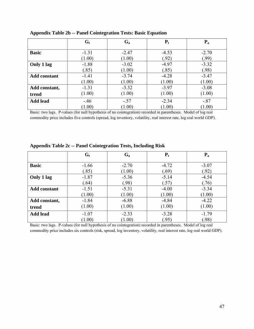
  47

Appendix Table 2b -- Panel Cointegration Tests: Basic Equation

Gt Ga Pt Pa

Basic -1.31 (1.00)

-2.47 (1.00)

-4.53 (.92)

-2.70 (.99)

Only 1 lag -1.88 (.85)

-3.02 (1.00)

-4.97 (.85)

-3.32 (.98)

Add constant -1.41 (1.00)

-3.74 (1.00)

-4.28 (1.00)

-3.47 (1.00)

Add constant, trend

-1.31 (1.00)

-3.32 (1.00)

-3.97 (1.00)

-3.08 (1.00)

Add lead -.46 (1.00)

-.57 (1.00)

-2.34 (1.00)

-.87 (1.00)

Basic: two lags. P-values (for null hypothesis of no cointegration) recorded in parentheses. Model of log real commodity price includes five controls (spread, log inventory, volatility, real interest rate, log real world GDP). Appendix Table 2c -- Panel Cointegration Tests, Including Risk

Gt Ga Pt Pa

Basic -1.66 (.85)

-2.70 (1.00)

-4.72 (.69)

-3.07 (.92)

Only 1 lag -1.87 (.64)

-5.36 (.98)

-5.14 (.57)

-4.54 (.76)

Add constant -1.51 (1.00)

-5.31 (1.00)

-4.00 (1.00)

-3.34 (1.00)

Add constant, trend

-1.84 (1.00)

-6.88 (1.00)

-4.84 (1.00)

-4.22 (1.00)

Add lead -1.07 (1.00)

-2.33 (1.00)

-3.28 (.95)

-1.79 (.98)

Basic: two lags. P-values (for null hypothesis of no cointegration) recorded in parentheses. Model of log real commodity price includes six controls (risk, spread, log inventory, volatility, real interest rate, log real world GDP).

  48

Appendix Table 3: Cointegration Vector Estimates from Commodity-Specific VECs Real World

GDP +

Volatility +

Spot-Fut. Spread

-

Inventories -

Real Int rate -

Corn -.28 (.21)

3.65** (1.04)

-.056** (.004)

-.47* (.20)

.03 (.03)

Copper .99** (.27)

-.37 (1.54)

-.076** (.007)

-.40* (.16)

-.04 (.05)

Cotton -.92** (.19)

5.75** (.95)

-.054** (.003)

-.91** (.24)

.01 (.03)

Cattle 6.20** (1.76)

-72** (10)

-.095** (.023)

17.2** (6.6)

.08 (.17)

Hogs -.09 (.27)

17.1** (2.7)

-.032** (.004)

-4.9** (1.2)

.02 (.03)

Oats -.54 (.31)

9.6** (2.1)

-.035** (.005)

.18 (.21)

.03 (.03)

Oil -5.0 (3.6)

20.2** (3.7)

-.15** (.01)

18. (12.)

-.02 (.19)

Platinum -1.9 (1.0)

10.0 (5.8)

.081** (.010)

.01 (.19)

.15 (.09)

Silver -2.1** (.3)

4.6** (.6)

-.043** (.003)

-.89** (.13)

.01 (.02)

Soybeans 1.54 (.79)

.64 (2.15)

-.135 (.009)

-.39 (.34)

.07 (.06)

Wheat -.69** (.14)

4.44** (.64)

-.039** (.003)

-.39 (.20)

.03 (.02)

Annual data. ** (*) ≡ significantly different from zero at .01 (.05) level. Standard errors in parentheses; Intercept and linear time trend included, not reported. VEC estimation, commodity by commodity, one lag.