Detection of Pulsars @ 21cm Jean-Jacques MAINTOUX - F1EHN

Pulsar : “Pulsating star”

Table of Contents

1 Signal Research and Choice of Techniques : ......................................................................................... 2

1.1 Evaluation : First Reception Test ................................................................................................... 2

1.2 Effect of Scintillation ..................................................................................................................... 3

1.3 Effect of Dispersion ....................................................................................................................... 3

2 Modifications to the RT 21cm : ............................................................................................................. 3

2.1 Receiver Chain ............................................................................................................................... 3

2.2 Signal Processing and Detection : .................................................................................................. 5

3 Pulsar@home (Simulated Pulsar) : ........................................................................................................ 6

3.1 Testing of the RF/IF Section ........................................................................................................... 6

3.2 Testing of the Detector .................................................................................................................. 6

3.3 Signal Processing ........................................................................................................................... 7

4 First Test on the RT @ 21cm : ................................................................................................................ 9

4.1 Sampling Clock Accuracy ............................................................................................................... 9

4.2 Doppler Effect ................................................................................................................................ 9

5 Observation of B0329+54 – Pulsar #1 : ............................................................................................... 10

6 Observation of B0950+08 – Pulsar #2 : ............................................................................................... 13

7 Observation of B1133+16 – Pulsar #3 : ............................................................................................... 16

8 Observation of B2020+28 – Pulsar #4 ................................................................................................. 19

8.1 Radiotelescope evolution ............................................................................................................ 19

8.2 Detection of B2020+28 ................................................................................................................ 19

9 Conclusions and Future Developments : ............................................................................................. 22

Rev 3 - 20 Mars 2017 - JJ MAINTOUX F1EHN

1 Signal Research and Choice of Techniques : The different pulsars identified by the scientific community are listed in various databases. I used the ATNF database http://www.atnf.csiro.au/research/pulsar/psrcat/ and the well-documented and detailed website Neutron-Star Group http://neutronstar.joataman.net/ dedicated to amateur observation of these objects. This site also includes tools to help enthusiasts in this adventure ... and this adventure is one that I will try to detail in what follows.

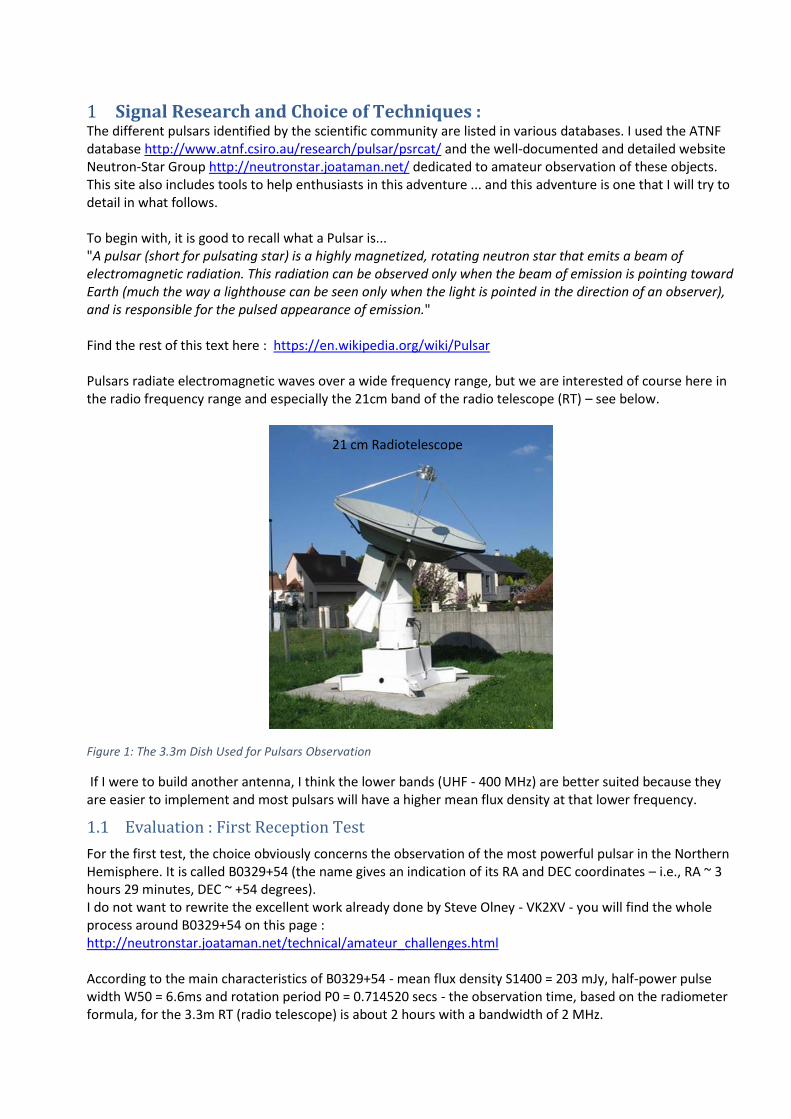
To begin with, it is good to recall what a Pulsar is... "A pulsar (short for pulsating star) is a highly magnetized, rotating neutron star that emits a beam of electromagnetic radiation. This radiation can be observed only when the beam of emission is pointing toward Earth (much the way a lighthouse can be seen only when the light is pointed in the direction of an observer), and is responsible for the pulsed appearance of emission." Find the rest of this text here : https://en.wikipedia.org/wiki/Pulsar Pulsars radiate electromagnetic waves over a wide frequency range, but we are interested of course here in the radio frequency range and especially the 21cm band of the radio telescope (RT) – see below.

Figure 1: The 3.3m Dish Used for Pulsars Observation

If I were to build another antenna, I think the lower bands (UHF - 400 MHz) are better suited because they are easier to implement and most pulsars will have a higher mean flux density at that lower frequency.

1.1 Evaluation : First Reception Test

For the first test, the choice obviously concerns the observation of the most powerful pulsar in the Northern Hemisphere. It is called B0329+54 (the name gives an indication of its RA and DEC coordinates – i.e., RA ~ 3 hours 29 minutes, DEC ~ +54 degrees). I do not want to rewrite the excellent work already done by Steve Olney - VK2XV - you will find the whole process around B0329+54 on this page : http://neutronstar.joataman.net/technical/amateur_challenges.html According to the main characteristics of B0329+54 - mean flux density S1400 = 203 mJy, half-power pulse width W50 = 6.6ms and rotation period P0 = 0.714520 secs - the observation time, based on the radiometer formula, for the 3.3m RT (radio telescope) is about 2 hours with a bandwidth of 2 MHz.

21 cm Radiotelescope

The first trial was conducted with the unmodified RT at 21cm. This test was negative 2 times. After research, it seems that the main cause is the very strong scintillation effect for this pulsar.

1.2 Effect of Scintillation

I learned that a very important feature of pulsars is scintillation. This effect is due to destructive and constructive interference of signals passing through the interstellar medium and the atmosphere. If constructive interference is your friend during an observation, a positive result can be obtained. However, if destructive interference is present, for a small antenna, there will likely be a poor or negative result.

Figure 2: Scintillation B0329+54 – Measured by DL0SHF

The image above (measurements by DL0SHF - http://sat-sh.lernnetz.de/pulsarsE.html ) shows the impact of scintillation on the amplitude of the B0329+54 signal. We now understand that detection with a small antenna takes some luck. To have the maximum chance of detecting B0329+54, it is necessary to increase the sensitivity of the RT to reduce the observation time. The only modifiable factor without rebuilding the RT antenna is bandwidth. However, not only is a practical bandwidth limit imposed by the receiver, but also by another important feature of pulsars: dispersion.

1.3 Effect of Dispersion

During passage through space, the broadband spectrum of the signal emitted by the pulsar is affected by the electron density of the interstellar medium. Lower frequencies are delayed compared to higher frequencies, which results in a smearing of the pulse and therefore a loss of signal. Please note this effect has an even greater impact on the lower bands. DM dispersion measurement is 26.76 cm 3 pc (parsec = pc) for B0329+54. Using the dispersion calculator http://neutronstar.joataman.net/technical/disp_del_calc.html , and fixing an upper limit on dispersion of the order of W50/2 = 3.5 ms, it is calculated that the frequency bandwidth can be increased to 50 MHz. With a bandwidth 25 times larger than 2 MHz, the observation time to detect B0329 + 54 at the same SNR is 25 times shorter and is of the order of 5 minutes (sqrt (BW * Tau) = constant). However, the recording time will remain unchanged because it must "thwart" scintillation and therefore take advantage of favorable moments that should enable faster detection. However, the transition to 50 MHz is not without impact on the RT architecture and care must be taken to avoid a time spreading of the pulse (which will cause a loss of signal). Please note, again, this effect has an even greater impact on the lower bands.

2 Modifications to the RT 21cm :

2.1 Receiver Chain

The intermediate frequency (IF) bandwidth is 50 MHz. Its center frequency and IF filters are designed to cover from 15 to 65 MHz (40 MHz center frequency). The local oscillator is also adapted to the new IF to down-convert the RF band 1427 +/- 25MHz. The RF front end is not impacted (the bandwidth of the 21cm filter is 50 MHz). RF image rejection is not impacted.

Figure 3: Receiver Chain

With 50 MHz, it is difficult at the amateur level to find a cheap SDR digital receiver. The solution is to use a basic broadband detector suitable for pulsars. To avoid complexity, the task of synchronization to the pulsar period is dedicated to digital processing (see below).

The solution is inspired by the reception chain used by DL0SHF, but the power meter is replaced with an RF detector quadratic response (square-law detector) type HP8472A, followed by an RC integrator of around 1ms.

The signal is then amplified by an operational amplifier type AD826. Finally, the signal is digitized by an ADC (16-bit) performed using a Teensy 3.2 (Arduino like). I used an application "Oscilloscope" adapted to this module and controlled by Matlab described here : http://www.mccauslandcenter.sc.edu/crnl/oscilloscope

Figure 4 : ADC Module - 16 bits

The various modifications described above therefore lead to the structure shown by the following diagram.

Figure 5: Pulsar Receiver Architecture

Data is sampled at 1 kHz (1ms period) and is stored on disk to allow processing at a later time. The processing also provides time synchronization to the period of the pulsar to perform synchronous detection.

The critical feature of the receiver is the stability and accuracy of this clock (1ms). Stability of the order of 0.2 ppm (less than 1.5ms error over 2 hours) is required to maintain a perfect synchronization of the duration of the recording. The accuracy allows determination of the period of the pulsar accurately as possible.

2.2 Signal Processing and Detection :

The data is a series of 16-bit samples clocked at 1ms. The processing is relatively simple to perform. It could be done using Excel, Octave, Scilab, Python .... I chose Matlab out of habit and for its graphical output. The principle of processing for detection is presented by the graph below.

Figure 6: Overall Detail of Processing

It allows presenting data in 2 ways:

➢ In a raster view composed of different frames (or frame). This view shows the evolution of the signal in function of time.

➢ An overview of the folded period. Then we can assess the temporal aspect of the pulsar signal.

The parameters X bins/period, duration of each frame and number of folded pulses are selected according to the details that are desired to be revealed (and according to the SNR of the pulsar observed). These tricks designed to enhance the functionality of the processing have been suggested to me by Joachim Köppen DF3GJ of the DL0SHF team. Many exchanges with Joachim also allowed me to benefit from his experience (see his website). Important : Only known pulsars and the most powerful are detectable by means of amateur (antenna of a few meters) by implementing this synchronous detection based on the scientific knowledge of the pulsar parameters.

3 Pulsar@home (Simulated Pulsar) : Following these first two negative tests, a simulated "Pulsar" was built to bench test the system before commissioning in the RT itself.

This bench test setup is used to test the modified RF part, detection and processing.

3.1 Testing of the RF/IF Section

This is an easy test and is done by implementing a sweep 1.4 / 1.5 GHz and noting the transfer function of the chain with a spectrum analyzer.

Figure 7: Measurement of the IF Signal (Bw=50MHz)

The result is nominal and off-band rejection is correct. The response is flat and the gain is sufficient for detection.

3.2 Testing of the Detector

To test the detector, the bench test below is performed using a pulsed noise diode followed by a variable attenuator of 0 to 40 dB so as to simulate a pulsar signal, firstly at a high level for testing the detection and integration, and secondly, at a low level to simulate and validate the pulsar processing.

Figure 8: Bench Test RF Pulse

The receiver is then bench tested (see below, receiver on the left, the IF module and detector in the center, underneath is the LO). The receiver incorporates a 12x multiplier to generate the LO. Detection can then be

tested using an oscilloscope to check the quality of detection as well as the integration constant. The detected signal is adjusted with an offset of 1.6V to lie within the 0 – 3.3V input range of the 16-bit ADC.

Figure 9: Detection Test with a Simulated PSR Signal

The entire chain is tested from an analog point of view by applying the appropriate signals.

3.3 Signal Processing

The calculation below sets the pulse generator settings to simulate a real signal to test the complete chain including signal processing.

For PSR B0329+54, the expected antenna temperature is 0.038K for Tsys system temperature of 65K or a ratio of 58.4E-05. In the lab, To = 290K and Tsys = 350 K, we must simulate a signal (Tsys*ratio) of 0.204K or 290.2K or ENR -32.3dB.

Period P= 0.72 s

Pulse @ 50% W50= 0.01 s

Peak flux Sc= (P / W50) mean flux

Freq Flux (Jy)

MHz Mean Peak

1400 0.2 24 Bw = 50 MHz

Signal level

Antenna Effective area 4.4 m²

Tantenna 0.04 K 5.24E-024 W/Hz

Trec 60 K -202.81 dBm/Hz

Tsky 5 K -125.82 dBm

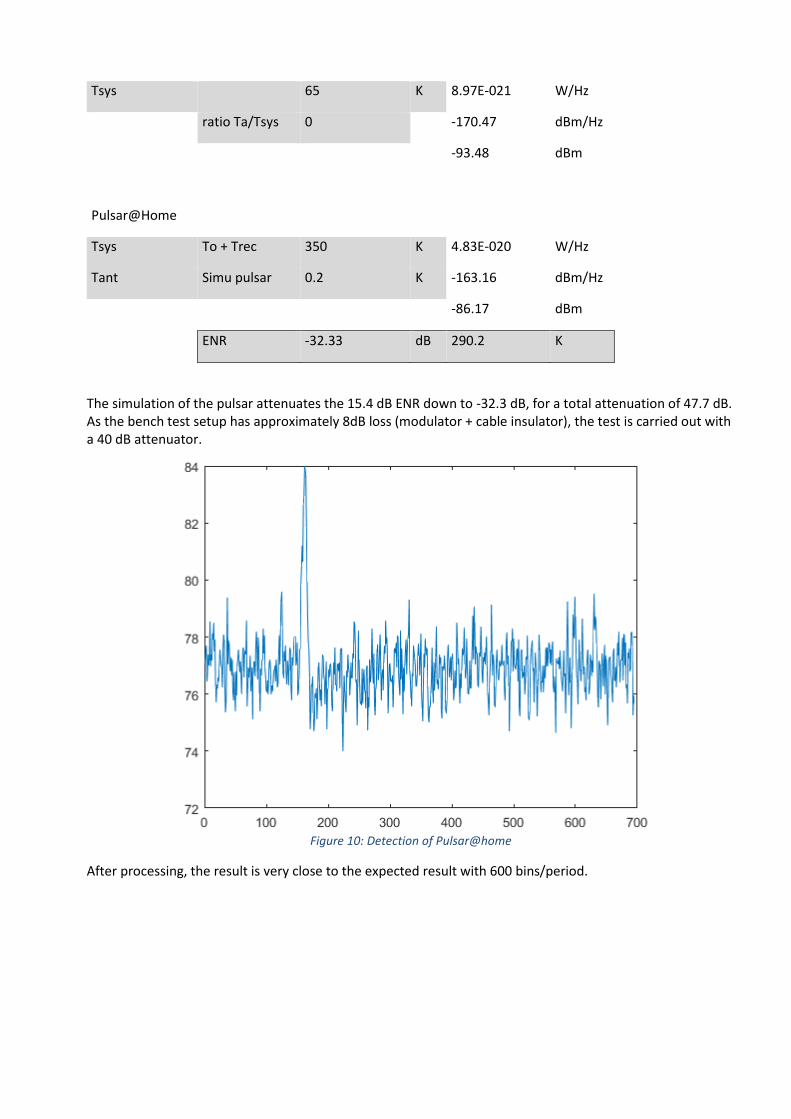
Tsys 65 K 8.97E-021 W/Hz

ratio Ta/Tsys 0 -170.47 dBm/Hz

-93.48 dBm

Pulsar@Home

Tsys To + Trec 350 K 4.83E-020 W/Hz

Tant Simu pulsar 0.2 K -163.16 dBm/Hz

-86.17 dBm

ENR -32.33 dB 290.2 K

The simulation of the pulsar attenuates the 15.4 dB ENR down to -32.3 dB, for a total attenuation of 47.7 dB. As the bench test setup has approximately 8dB loss (modulator + cable insulator), the test is carried out with a 40 dB attenuator.

Figure 10: Detection of Pulsar@home

After processing, the result is very close to the expected result with 600 bins/period.

4 First Test on the RT @ 21cm : A recording of about 2 hours was carried out in pursuit of B0329+54 on April 3, 2016. The figure below shows the B0329+54 signal, with the Y-axis showing 140 frames each of of 2 mins integration, and X-axis equal to the period of the pulsar in milliseconds obtained by a TEMPO calculation.

Figure 11: First Detection of B0329+54

Despite an imperfect estimate of the period of the pulsar, it is found that detection is evident. The incorrect setting of the folding period results in a temporal drift across the recording compared to the reference period. This observation brings two very important comments.

4.1 Sampling Clock Accuracy

This feature has already been discussed above. In addition to stability, the sampling clock has to be accurate because it is the reference for the folding of the different samples. If the clock is incorrect, at the time of measurement, the samples are assigned to the wrong box (phase) of the period of the pulsar. So this shift is observed. This is not a problem for strong signal, but it would become a problem for a weaker signal (the processing gain on all the samples would not be accessible because of this delay spread).

Compared to the expected period, we see that the sampling frequency is shifted by 20 ppm. This error is due to the accuracy of the Teensy 3.2 clock. This factor will be used in future observations to correct the observed periods.

4.2 Doppler Effect

This effect is not important for the pulsar radio signal itself since its spectrum signal is broadband and no Doppler processing is performed.

However, this effect has a significant impact on the observed period of the pulsar. Because the period information sought is important, the shift in apparent period caused by the Doppler effect is not at all negligible. Software such as TEMPO or PRESTO (based on TEMPO) used to calculate the observed period take into account all the Doppler components of the relative velocity of the pulsar in the Earth's rotation.

It was Wolfgang Hermann (Astropeiler Stockert in Germany) who calculated for me all the periods needed for my various observations.

5 Observation of B0329+54 – Pulsar #1 : A second test conducted on April 24 led to a positive result very similar to the first. Now the RT is fully functional and this test is detailed in this section. The figure below shows the evolution of the pulsar signal versus time. The waterfall shows 75 frames of 2 minutes (120sec)

Figure 12: Detection of B0329+54 as a Function of Time

Note that the clock deviation is corrected. The observation is perfectly synchronized with the topocentric period of the pulsar. The scintillation effect is marked in the same manner as in the previous recording, revealing a relatively "strong" signal on the first 15 frames (approx 30min), then a low signal on the next 10 frames and then fading on the 15 following frames (25 to 40). The rest of the record remains at a low level, but note that here the observation time is 2 minutes per frame. The report provides 5 min with 50 MHz band which shows proper operation and very close to the expected result.

If one folds the whole sample over a period, then the S/N ratio (SNR) is very favorable as shown in the figure below with a resolution of 100 bins/period.

Figure 13: A Single Integrated Pulse - 100 bins/period

With such a strong signal, it is possible to change the processing parameters from 100 bins/period to 700 bins/period to improve the time resolution and refine the details.

Figure 14: A Single Integrated Pulse - 700 bins/period

This new graphic then shows the presence of a pre- and post-pulse at the base of the main pulse. This feature of this pulsar is already known. Here the view is the normal mode where the post-pulse is greater than the pre-pulse. It represents 80% of the signal. The remaining 20% could not be observed.

According to experts, the presence of pre- and post-pulses reveals changes in the chemical composition and the pulsar's surface structure. See http://adsabs.harvard.edu/abs/1982ApJ...258..776B

With this SNR it is possible to trace a succession of pulses. The figure below shows the stability of the normal mode observed. Pre- and post-pulses are perfectly visible.

Figure 15: 2 Integrated Pulses - 700bins/period

For fun, I analyzed a sequence of many pulses and used the detection envelope to modulate a synthetic sound to recreate an audio signal representing the reception of the pulsar. The file is here: https://www.youtube.com/watch?v=WbHWxLmAy4k&feature=em-share_video_user

Figure 16: 4 Integrated Pulses – Audio Modulation

The changing details of this pulse sequence might suggest a mode change, but the signal to noise ratio is not sufficient to reach such a conclusion.

6 Observation of B0950+08 – Pulsar #2 : This pulsar is the second most powerful in the Northern Hemisphere. Its main features are: mean flux density = 84 mJy S1400, half-power pulse width W50 = 9.5 ms and rotation period P0 = 0.253065 sec.

The dispersion of B0950+08 is very small and negligible in this test compared to the width of the pulse.

The figure below shows the evolution of the B0950+08 signal versus time. The X-axis corresponds to the period of the pulsar, and the Y-axis corresponds to 3 hours recording time (180 min) cut into 9 frames each of 1200 sec duration (20 min). The frame 7 reveals a period of unusable signal due to a technical problem on the RT with the tracking system.

Figure 17:Waterfall 9 Frames of 20 min

The measured period (obtained by finding the maximum signal to noise ratio - max SNR) is 253.0739 ms. After correcting the sampling clock error of 20 ppm, the measured period of the pulsar is 253.0789 ms is very close to the PRESTO calculation, namely 253.07884 ms.

One can also see that the signal is more stable over the duration of the recording. The scintillation of this pulsar is lower, probably due to a smaller distance of about 850 Ly (compared with 3460 Ly for B0329+54) after a review of Wolfgang.

The figure below shows the period of the pulsar folded over the entire recording with a resolution of 50 bins/period.

Figure 18: B0950+08 - 1 Integrated Pulse – 50 bins/period

The SNR obtained improves the resolution and the figure below shows the same period with a resolution of 500 bins / period.

Figure 19: B0950+08 - 1 Integrated Pulse – 500 bins/period

This figure then reveals the presence of a shoulder into the left flank of the pulse of B0950+08. The asymmetric profile of this pulsar seems to be known. This could reveal the presence of a second radio component and give details of the radiation characteristics of B0950+08. I say "could" because these analyses are well beyond my skills and my imagination. Here we are immersed in another world very different from our environment.

Zooming in on the previous figure allows checking the width of the pulse at half power W50.

Figure 20: B0950+08 - 1 Integrated Pulse – W50

Here W50 is of the order of 8 to 10 ms depending on whether we include the shoulder or not. It's very close to the expected value.

7 Observation of B1133+16 – Pulsar #3 : The choice of this pulsar was made on the basis of mean flux density in order to know the limits of the station and because its position allows observation during the summer day, which is more comfortable at the RT's location. Its dispersion is also very small and its effect is negligible.

The mean flux density of this pulsar is extremely low. This pulsar is the 6th most powerful of the Northern Hemisphere. Its main features are: mean flux density = 32 mJy S1400, half-power pulse width W50 = 31.7 ms and rotation period P0 = 1.187913 sec.

The figure below shows the evolution of the B1133+16 signal versus time. The X-axis corresponds to the period of the pulsar, and the Y-axis corresponds to 1.5 hours of recording time (90 min) cut into 8 frames of 713 seconds each (approx 12 min).

Figure 21: Waterfall 8 Frames of about 12 min

This figure shows the scintillation effect as predicted by Wolfgang's comments (Astropeiler Stockert). Over 60% of the time at the start of recording the pulsar is undetectable.

On the other hand, at the end of the recording the received level seems well above the expected level and shows a strong signal detection signal even during short frame of about 12 min..

The measured period is also very close to the topocentric period as calculated by PRESTO. The corrected observed value is 1187.99026 ms versus the calculated 1187.98948059 ms value.

The RT's sample rate is now fully corrected.

A second recording made with a longer duration gives exactly the same observation concerning the signal level and the effect of scintillation.

The figure below shows the period of the pulsar folded over the entire recording with a resolution of 150 bins/period (the period is longer than the previous pulsars and so more samples are needed to maintain proper temporal resolution).

Figure 22: B1133+16 - 1 Integrated Pulse – 150 bins/period

As expected, the signal to noise ratio is low and the limit of the current RT is reached.

However, the quality of the successful detection remains high. The principle of synchronous detection also eliminates a lot of spurious signals which could disrupt detection.

In addition, the pulse observed of B1133+16 seems narrower than the value of W50 = 31.7ms as found in the ATNF database. A test with a resolution of 750 bins/sec reveals details without altering the signal to noise ratio.

Figure 23: B1133+16 - 1 Integrated Pulse – 750 bins/period

The measured W50 pulse width is much lower than expected. Of the order of 10 ms compared to the 31.7ms contained in the ATNF database. Some Internet research led me to this paper http://arxiv.org/abs/1511.08298v2 . It publishes a graph of pulse profiles as a function of frequency as shown below.

It seems that at 21cm (1410 MHz), the radiation energy of the PSR is mostly contained in the main pulse. And of course, this pulse is narrower. According to the graph, which shows the main pulse at about 4 ° width in phase, equivalent to 13 ms (4*P0/360, where 360 ° corresponds to the period of the pulsar). This paper gives also an assumption about the double cone radiation structure and evokes the presence of a third component. It's impressive ... it's really another world!

Consulting the Astrospeiler Stockert detection results at 21cm also confirms the observed width of the pulse and the second component. http://astropeiler.de/sites/default/files/Pulsar_Observations_2015.pdf page 23

A final measure of this pulsar views the period of 2 consecutive folded pulses. Of course the signal to noise ratio is low but the period is clearly observed.

Figure 24: B1133+16 - 2 Integrated Pulses - 750bins/period.

8 Observation of B2020+28 – Pulsar #4 The choice of this pulsar was made for its average flux corresponding to the item #9 of the 21cm pulsar list available on the site Neutron Star, its position allowing a daytime observation in winter. Its dispersion is also low and its effect is negligible at 21cm.

The flux of this pulsar is very low. This pulsar is the 4th most powerful of the Northern Hemisphere but is known to have a significant scintillation (see below). Its main characteristics are: Average flux S1400 = 36 mJy, pulse width at half power W50 = 12 ms and Rotation period P0 = 0.343402 sec.

The simulations done for this pulsar shows that an SNR of 4 (6 dB) is obtained after at least 6 hours of integration. The first trials performed with the RT described at the beginning of this note were negative. The main causes of these failures are the presence of parasitic signals but mainly the stability of the clock which fluctuates according to the temperature (winter conditions). Moreover, the observation time being doubled, the stability must be improved.

8.1 Radiotelescope evolution

The main changes are around the Teensy module.

Spurious signals are injected via the USB power supply from the PC. To correct this, external power supply and regulator are implanted into the ADC (digitizer) unit, see § 2.1 Receiver Chain.

The Teensy oscillator is based on a crystal oscillator. To improve the Teensy stability, the quartz was removed and an external reference clock is injected onto the pin 22 of the MCU MK20DX256.

The 16 MHz reference clock is supplied with an GPS disciplined oscillator (GPSDO) and injected at 0 dBm instead of the quartz (pin 22).

Figure 25 : The Teensy module update

8.2 Detection of B2020+28

The figure below shows the evolution of the B2020 + 28 signal as a function of time. The X axis corresponds to the pulsar period, and the Y axis corresponds to the recording time of 7.5h (450 min) cut in 15 frames of 1800 sec (30 min).

Removing the crystal and injecting a reference Clock on pin 22

Figure 26: Waterfall 15 frames of 30 mn

As predicted, this figure shows the effect of scintillation mainly for frames 4 to 7 and from the 11th frame. At the end of the observation, the pulsar is no longer detectable over a period of 30 minutes. The effect of scintillation is detailed below.

The measured period is exactly the period the planned topocentric period and calculated using the new tool of the Neutron Star site (see references). The measured value is 343.393050 ms.

The figure below shows the period of the pulsar folded over the entire recording with a resolution of 64 bin / period (which is about ½ W50).

Figure 27: B2020+28 - 2 integrated pulses - 64 bin/période

As expected, the signal-to-noise ratio is low but in line with expectations. The detection quality is very good and allows to present a direct result over 2 periods as well as the following observations.

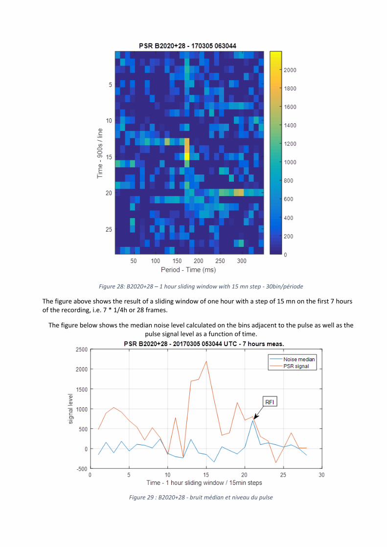
Figure 28: B2020+28 – 1 hour sliding window with 15 mn step - 30bin/période

The figure above shows the result of a sliding window of one hour with a step of 15 mn on the first 7 hours of the recording, i.e. 7 * 1/4h or 28 frames.

The figure below shows the median noise level calculated on the bins adjacent to the pulse as well as the pulse signal level as a function of time.

Figure 29 : B2020+28 - bruit médian et niveau du pulse

We can observe the effect of scintillation on the PSR signal level. On average value, the signal level corresponds to the expected PSR average flux. Positive scintillations compensate well for negative scintillation instants.

A last processing is dedicated to reveal the profile of the pulsar. Its W50 width is nominal.

Figure 30 : Profil du pulsar B2020+28

The profile observed conforms to the profile available in the ATNF database below. At 21cm, the average pulse profile of the PSR B2020+28 is relatively simple, having 2 main emission components well resolved, which seems common according to the experts (https://arxiv.org/pdf/1605.06622.pdf).

Figure 31 : Profil PSR B2020+28 - Base ATNF

9 Conclusions and Future Developments : Changes to the RT 21cm helped catch reliable and reproducible pulsar signals. The technical solution is really easy and synchronization efforts are processed by software. The stability of the digitizing clock, here that of the Teensy 3.2, has been improved and now allows long recordings, very stable and very precise. These improvements made it possible to detect B2020+28 having a low mean flux.

The data processing eliminates interfering signals and synchronous detection makes them more robust results to specific pests such as road traffic. The results are very similar to those found in the literature and can reveal certain characteristics of pulsars. Again, the RT was able to detect extremely weak signals and a new challenge has been raised after the difficult observation of M31. (See results on my website). These results are also due to some people I want to again thank for their help, support and exchange of information: René Keller, Joachim Köppen, DF3GJ of the DL0SHF team, Wolfgang Hermann (Astropeiler Stockert), Steve Olney VK2XV and Damien Boureille. With the detection of B2020+28, other detections are possible. Other developments are coming on the RT. They will probably equip it with a broadband SDR to access a de-spread function to correct the effects of dispersion. This function will be mandatory for some pulsars where the dispersion leads to a delay spread more than the duration of the pulse.

References :

Some websites that contain a lot of information http://neutronstar.joataman.net/ http://neutronstar.joataman.net/technical/rel_flux_density.html http://neutronstar.joataman.net/technical/radiometer_eqn.html http://sat-sh.lernnetz.de/pulsarsE.html http://sat-sh.lernnetz.de/pulsarsDetailsE.html http://astropeiler.de http://astropeiler.de/sites/default/files/Pulsar_Observations_2015.pdf http://www.atnf.csiro.au/research/pulsar/psrcat/ RT 21cm - our Galaxy @ 21cm : http://www.youtube.com/watch?v=HGwkZY4E64k My website. http://www.f1ehn.org page “radioastro”.

You can contact me via email jj@f1ehn.org or jjm_f1ehn@wanadoo.fr

English version translated by Steve Olney.