Embed Size (px)
Citation preview

1
Title: Detecting the impact of temperature on transmission of Zika, dengue and 1
chikungunya using mechanistic models 2
3
Short title: Temperature predicts Zika, dengue, and chikungunya transmission 4
Authors: Erin A. Mordecaia*, Jeremy M. Cohenb, Michelle V. Evansc, Prithvi Gudapatia, Leah 5
R. Johnsonb, Catherine A. Lippic, Kerri Miazgowiczd, Courtney C. Murdockd,e, Jason R. Rohrb, 6
Sadie J. Ryanc,f,g,h, Van Savagei,j, Marta S. Shocketa,k, Anna Stewart Ibarral, Matthew B. 7
Thomasm, Daniel P. Weikeln 8
Affiliations: 9
aBiology Department, Stanford University, 371 Serra Mall, Stanford, CA 94305 10
bDepartment of Integrative Biology, University of South Florida, 4202 East Fowler Ave, 11
SCA110 Tampa, FL 33620 12
cDepartment of Geography, University of Florida, PO Box 117315, Turlington Hall, Gainesville, 13
FL 32611 14
dCenter for Tropical and Emerging Global Disease, Department of Infectious Diseases, 15
University of Georgia College of Veterinary Medicine, 501 D.W. Brooks Drive, Athens, GA 16
30602 17
eOdum School of Ecology, University of Georgia, 140 E. Green St., Athens, GA 18
30602fEmerging Pathogens Institute, University of Florida, P.O. Box 100009, 2055 Mowry Road 19
Gainesville, FL 32610 20
gCenter for Global Health and Translational Science, Department of Microbiology and 21
Immunology, Weiskotten Hall, SUNY Upstate Medical University, Syracuse, NY 13210 22

2
hSchool of Life Sciences, College of Agriculture, Engineering, and Science, University of 23
KwaZulu Natal, Private Bag X01, Scottsville, 3209, KwaZulu Natal, South Africa 24
iDepartment of Ecology and Evolutionary Biology, University of California Los Angeles and 25
Department of Biomathematics, University of California Los Angeles, Los Angeles, CA 90095 26
jSanta Fe Institute, 1399 Hyde Park Rd, Santa Fe, NM 87501 27
kDepartment of Biology, Indiana University, 1001 E. 3rd St., Jordan Hall 142, Bloomington, IN 28
47405 29
lCenter for Global Health and Translational Sciences, SUNY Upstate Medical University, 30
Syracuse, NY13210 31
mDepartment of Entomology and Center for Infectious Disease Dynamics, Penn State University, 32
112 Merkle Lab, University Park, PA 16802 33
nDepartment of Biostatistics, University of Michigan, 1415 Washington Heights, Ann Arbor, MI 34
48109 35
*Correspondence to: Erin Mordecai. Biology Department, Stanford University, 371 Serra Mall, 36
Stanford, CA 94305. (650) 497-7447. [email protected] 37
Keywords: Zika, dengue, chikungunya, temperature, vector transmission, Aedes aegypti, Aedes 38
albopictus 39
40
41

3
Abstract 42
Recent epidemics of Zika, dengue, and chikungunya have heightened the need to understand the 43
seasonal and geographic range of transmission by Aedes aegypti and Ae. albopictus mosquitoes. 44
We use mechanistic transmission models to derive predictions for how the probability and 45
magnitude of transmission for Zika, chikungunya, and dengue change with mean temperature, 46
and we show that these predictions are well matched by human case data. Across all three 47
viruses, models and human case data both show that transmission occurs between 18-34°C with 48
maximal transmission occurring in a range from 26-29°C. Controlling for population size and 49
two socioeconomic factors, temperature-dependent transmission based on our mechanistic model 50
is an important predictor of human transmission occurrence and incidence. Risk maps indicate 51
that tropical and subtropical regions are suitable for extended seasonal or year-round 52
transmission, but transmission in temperate areas is limited to at most three months per year even 53
if vectors are present. Such brief transmission windows limit the likelihood of major epidemics 54
following disease introduction in temperate zones. 55
56
Author Summary (150-200 words) 57
Understanding the drivers of recent Zika, dengue, and chikungunya epidemics is a major public 58
health priority. Temperature may play an important role because it affects mosquito 59
transmission, affecting mosquito development, survival, reproduction, and biting rates as well as 60
the rate at which they acquire and transmit viruses. Here, we measure the impact of temperature 61
on transmission by two of the most common mosquito vector species for these viruses, Aedes 62
aegypti and Ae. albopictus. We integrate data from several laboratory experiments into a 63
mathematical model of temperature-dependent transmission, and find that transmission peaks at 64

4
26-29°C and can occur between 18-34°C. Statistically comparing model predictions with recent 65
observed human cases of dengue, chikungunya, and Zika across the Americas suggests an 66
important role for temperature, and supports model predictions. Using the model, we predict that 67
most of the tropics and subtropics are suitable for transmission in many or all months of the year, 68
but that temperate areas like most of the United States are only suitable for transmission for a 69
few months during the summer (even if the mosquito vector is present). 70
71

5
Main Text 72
Epidemics of dengue, chikungunya, and Zika are sweeping through the Americas, and are part of 73
a global public health crisis that places an estimated 3.9 billion people in 120 countries at risk 74
[1]. Dengue virus (DENV) distribution and intensity in the Americas has increased over the last 75
three decades, infecting an estimated 390 million people (96 million clinical) per year [2]. 76
Chikungunya virus (CHIKV) emerged in the Americas in 2013, causing 1.8 million suspected 77
cases from 44 countries and territories (www.paho.org). In the last two years, Zika virus (ZIKV) 78
has spread throughout the Americas, causing 714,636 suspected and confirmed cases, with many 79
more unreported (http://ais.paho.org/phip/viz/ed_zika_cases.asp, as of January 5, 2017). The 80
growing burden of these diseases (including links between Zika infection and both microcephaly 81
and Guillain-Barré syndrome [3]) and potential for spread into new areas creates an urgent need 82
for predictive models that can inform risk assessment and guide interventions such as mosquito 83
control, community outreach, and education. 84
Predicting transmission of DENV, CHIKV, and ZIKV requires understanding the 85
ecology of the vector species. For these viruses the main vector is Aedes aegypti, a mosquito that 86
prefers and is closely affiliated with humans, while Ae. albopictus, a peri-urban mosquito, is an 87
important secondary vector [4,5]. We expect one of the main drivers of the vector ecology to be 88
the climate, particularly temperature. For that reason, mathematical and geostatistical models that 89
incorporate climate information have been valuable for predicting and responding to Aedes spp. 90
spread and DENV, CHIKV, and ZIKV outbreaks [5–10]. 91
The effects of temperature in ectotherms are largely predictable from fundamental 92
metabolic and ecological processes. Survival, feeding, development, and reproductive rates 93
predictably respond to temperature across a variety of ectotherms, including mosquitoes [11,12]. 94

6
Because these traits help to determine transmission rates, the effects of temperature on 95
transmission should also be broadly predictable from mechanistic models that incorporate 96
temperature-dependent traits. Here, we introduce a model based on this framework that 97
overcomes several major gaps that currently limit our understanding of climate suitability for 98
transmission. Specifically, we develop models of temperature-dependent transmission for Ae. 99
aegypti and Ae. albopictus that are (a) mechanistic, facilitating extrapolation beyond the current 100
disease distribution, (b) parameterized with biologically accurate unimodal thermal responses for 101
all mosquito and virus traits that drive transmission, and (c) validated against human dengue, 102
chikungunya, and Zika case data across the Americas. 103
We synthesize available data to characterize the temperature-dependent traits of the 104
mosquitoes and viruses that determine transmission intensity. With these thermal responses, we 105
develop mechanistic temperature-dependent virus transmission models for Ae. aegypti and Ae. 106
albopictus. We then ask whether the predicted effect of temperature on transmission is consistent 107
with patterns of actual human cases over space and time. To do this, we validate the models with 108
DENV, CHIKV, and ZIKV human incidence data at the country scale from the Americas from 109
2014-2016. To isolate temperature dependence, we also statistically controlled for population 110
size and two socioeconomic factors that may influence transmission. If temperature 111
fundamentally limits transmission potential, transmission should only occur at actual 112
environmental temperatures that are predicted to be suitable, and conversely, areas with low 113
predicted suitability should have low or zero transmission (i.e., false negative rates should be 114
low). By contrast, low transmission may occur even when temperature suitability is high because 115
other factors like vector control can limit transmission (i.e., the false positive rate should be 116
higher than the false negative rate). Finally, if the simple mechanistic model accurately predicts 117

7
climate suitability for transmission, then we can use it to map climate-based transmission risk of 118
DENV, CHIKV, ZIKV, and other emerging pathogens transmitted by Ae. aegypti and Ae. 119
albopictus seasonally and geographically. 120
Results 121
Temperature-dependent transmission 122
Data gathered from the literature [9,13–15,15–21,21–30] revealed that all mosquito traits 123
relevant to transmission—biting rate, egg-to-adult survival and development rate, adult lifespan, 124
and fecundity—respond strongly to temperature and peak between 23°C and 34°C for the two 125
mosquito species (Ae. aegypti in Fig. 1 and Ae. albopictus in Fig. S1). DENV extrinsic 126
incubation and vector competence peak at 35°C [31–37] and 31-32°C [31,32,34,38], 127
respectively, in both mosquitoes—temperatures at which mosquito survival is low, limiting 128
transmission potential (Figs. 1, S1). Appropriate thermal response data were not available for 129
CHIKV and ZIKV extrinsic incubation and vector competence. 130
131
Fig. 1. Thermal responses of Ae. aegypti and DENV traits that drive transmission (data sources 132
listed in Table S2). Informative priors based on data from additional Aedes spp. and flavivirus 133
studies helped to constrain uncertainty in the model fits (see Materials and Methods; Table S3). 134
Points and error bars indicate the data means and standard errors (for display only; models were 135
fit from the raw data). Black solid lines are the mean model fits; red dashed lines are the 95% 136
credible intervals. Thermal responses for Ae. albopictus are shown in Fig. S1. 137
138

8
We estimated the posterior distribution of R0(T) and used it to calculate key temperature 139
values that indicate suitability for transmission: the mean and 95% credible intervals (95% CI) 140
on the critical thermal minimum, maximum, and optimum temperature for transmission by the 141
two mosquito species. At constant temperature, Ae. aegypti transmission peaked at 29.1°C (95% 142
CI: 28.4 – 29.8°C), and declined to zero below 17.8°C (95% CI: 14.6 – 21.2°C) and above 143
34.6°C (95% CI: 34.1 – 35.6°C) (Fig. 2). Ae. albopictus transmission peaked at 26.4°C (95% CI: 144
25.2 – 27.4°C) and declined to zero below 16.2°C (95% CI: 13.2 – 19.9°C) and above 31.6°C 145
(95% CI: 29.4 – 33.7°C) (Fig. 2). Overall, the thermal response curve for Ae. albopictus is 146
shifted towards lower temperatures than Ae. aegypti, so Ae. albopictus transmission is better 147
suited to colder environments. For a more realistic scenario in which daily temperature ranged 148
over 8°C, the transmission peak, minimum, and maximum were slightly lower for both Ae. 149
aegypti (28.5°C, 13.5°C, 34.2°C, respectively) and Ae. albopictus (26.1°C, 11.9°C, and 28.3°C, 150
respectively). The lower thermal maximum under fluctuating temperatures occurs because we 151
incorporated empirically supported irreversible lethal effects of temperatures that exceed thermal 152
maxima for survival (see Materials and Methods). 153
154
Fig. 2. Relative R0 across constant temperatures (°C; top) for Ae. albopictus (light blue) and Ae. 155
aegypti (dark blue), and histograms of the posterior distributions of the critical thermal minimum 156
(bottom left), temperature at peak transmission (bottom middle), and critical thermal maximum 157
(bottom right; all in °C). Solid lines: mean posterior estimates; dashed lines: 95% credible 158
intervals. R0 curves normalized to a 0-1 scale for ease of comparison and visualization. 159
160

9
The posterior distribution of R0(T) allows us to evaluate uncertainty in key temperature 161
values that define the transmission range, including critical thermal minimum, maximum, and 162
optimum. Uncertainty was higher for the critical thermal minimum for transmission than for the 163
maximum or optimum, and the two mosquito species overlapped most for this outcome (Fig. 2, 164
bottom panels). This occurred because several trait thermal responses increase gradually from 165
low to mid temperatures but decline more steeply at high temperatures (Fig. 1), so uncertainty is 166
greatest at low temperatures. Ae. aegypti has a substantially higher optimum and maximum 167
temperature than Ae. albopictus (Fig. 2) due to its greater rates of adult survival at high 168
temperatures (see Supplementary Materials for sensitivity analyses). 169
170
Model validation 171
We used generalized linear models (GLM) to ask whether the predicted relationship 172
between temperature and transmission, R0(T), was consistent with observed human cases of 173
DENV, CHIKV, and ZIKV. Specifically, we assessed whether R0(T) was an important predictor 174
of the probability of autochthonous transmission occurring and of the incidence given that 175
transmission occurred. We also controlled for human population size, virus species, and two 176
socioeconomic factors. (Note that we focused on testing the R0(T) model, rather than on 177
constructing the best possible statistical model of human case data.) To do this, we used the 178
version of the Ae. aegypti R0(T) model that includes 8°C daily temperature range, along with 179
country-scale weekly case reports of DENV, CHIKV, and ZIKV in the Americas and the 180
Caribbean between 2014-2016. We first addressed the fact that countries with larger populations 181
have greater opportunities for (large) epidemics by creating two predictors that incorporate 182
scaled R0(T) and population size. In the models of the probability of autochthonous transmission 183

10
occurring we used the product of the posterior probability that R0(T) > 0 (which we notate as 184
GR0) and the log of population size (p) to give log(p)*GR0. In the models of incidence given that 185
transmission does occur we used the log of the product of the posterior mean of R0(T) and 186
population size, log(p*R0(T)). To control for several socioeconomic factors that might obscure 187
the impact of temperature, we also included log of gross domestic product (GDP) and log percent 188
of GDP in tourism (using logs to improve normality). These are potential indicators of 189
investment in and/or success of vector control and infrastructure improvements that prevent 190
transmission. By comparing models that included the R0(T) metric alone, socioeconomic factors 191
alone, or both, we tested whether R0(T) was an important predictor of observed transmission 192
occurrence and incidence (see Table S4). Note that R0(T) is out of sample because it is derived 193
and calculated strictly from laboratory data on mosquitoes, and we perform a validation analyses 194
for R0(T) using independent case incidence reports. For this validation step we assessed model 195
adequacy for the transmission data in two ways. First we used the full dataset for case incidence 196
reports to select the best model (Table S4) and determine whether or not our predicted value of 197
relative R0(T) based on laboratory data was included in the model (“within sample” analysis). 198
Second we used a bootstrapping approach where models were fit on subsets of the case incidence 199
data that were randomly sampled and then predictive accuracy of the competing models (Table 200
S4) was assessed on left-out data (“out of sample” analysis). 201
For the probability of autochthonous transmission occurring, the model that included both 202
the R0(T) predictor and socioeconomic predictors had overwhelming support based on Bayesian 203
Information Criterion (BIC; model PA5 relative probability = 1, Table S4). Based on deviance 204
explained, the models that included R0(T), with or without the socioeconomic predictors out-205
performed the model that did not include R0(T) (Table S4; Figs. 3A, S2). In analyses of out-of-206

11
sample accuracy, models that included the R0(T) metric (with or without the socioeconomic 207
factors) were surprisingly accurate. They predicted the probability of transmission with 86-91% 208
out-of-sample accuracy for DENV (Table S4). For CHIKV and ZIKV, models that included the 209
R0(T) metric or population alone had 66-69% out-of-sample accuracy (Table S4). There were no 210
significant differences in out-of-sample accuracy between the top four models but for both 211
DENV and CHIKV/ZIKV the best model was significantly better than the worst model (see 212
Supplementary Code for full results). The lower out-of-sample accuracy for CHIKV and ZIKV 213
likely reflects the much lower frequency of positive values and the lower total sample size of this 214
dataset. All results were similar for a set of models that separated GR0 from population size, so 215
for simplicity we show the model predictors that combines GR0 and population size here (see 216
Table S4 and Supplementary Code for results of other models). Further, from a biological 217
perspective, the combined model better describes what we know about disease systems: if either 218
the probability of R0(T) being greater than zero is small or population size is very small, 219
transmission is unlikely to occur. Together, these analyses suggest that R0(T) is an important 220
predictor of transmission occurrence, but that CHIKV and ZIKV need further data to better 221
explain the probability of transmission occurrence (Figs. 3A, S2). 222
223
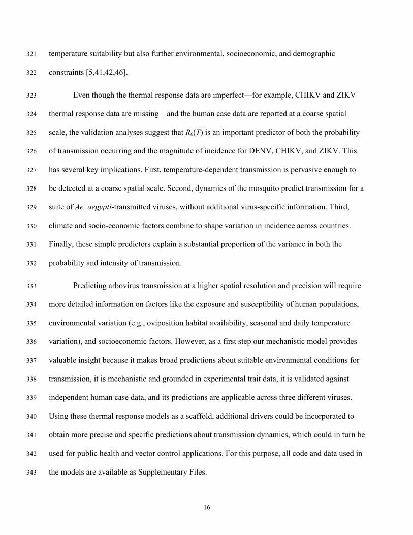
Fig. 3. Ae. aegypti R0(T) and population size predict the probability and magnitude of 224
transmission of DENV, CHIKV, and ZIKV across the Americas. A, log(p)*GR0 (the posterior 225
probability that R0(T) > 0 times the log of population size) versus the probability of local 226
transmission in the data. B, log(p*R0(T)) (log of R0(T) times the population size) versus the log 227
of incidence, given that it exceeds the threshold for local transmission. Tick-marks and points: 228
human transmission occurrence and incidence data, respectively, by country-week in the 229

12
Americas and Caribbean. Lines and shaded areas: mean and 95% CI from GLM fits for DENV 230
(blue) and CHIKV and ZIKV (red). For simplicity, we show the models that only include the 231
covariates log(p)*GR0 or log(p*R0(T)), respectively, and do not include the socioeconomic 232
covariates (models PA6 and IM4 in Table S4). For each case report data point, log(p)*GR0 and 233
log(p*R0(T)) were calculated at the mean temperature 10 weeks prior to the reporting week [39]. 234
235
R0(T) was also an important predictor of incidence, given that autochthonous 236
transmission did occur. Within-sample, incidence was best predicted by the model that included 237
both R0(T) and the socioeconomic predictors (model IM5 in Table S4) based on BIC (relative 238
probability = 1). The models that included R0(T) out-performed those that did not based on 239
deviance explained (Table S4). In out-of-sample validation, the models that included R0(T) 240
explained the magnitude of incidence based on mean absolute percentage error (85-86% 241
accuracy versus 83% accuracy for models that did not include R0(T); Table S4), but this 242
difference was not statistically significant. For illustration, we show the simpler model that only 243
contains the R0(T) predictor in the main text (Fig. 3B; model IM1 in Table S4). Notably, the 244
models that contained R0(T) predicted incidence well for all three viruses, despite the lower 245
incidence of CHIKV and ZIKV. 246
Although predicted R0(T) correlated with the observed occurrence and magnitude of 247
human incidence for all three viruses, these observed incidence metrics were higher for DENV 248
than for CHIKV and ZIKV. While the reason for this difference is unclear, the most likely 249
explanation is that DENV is much more established in the region, so it is more likely to be 250
detected, diagnosed, and reported. Because ZIKV and CHIKV are newly emerging, they may not 251
have fully saturated the region at this early stage. 252

13
The ability of the model to explain the probability and magnitude of transmission is 253
notable given the coarse scale of the human incidence versus mean temperature data (i.e., 254
country-scale means), the lack of CHIKV- and ZIKV-specific trait thermal response data to 255
inform the model, the nonlinear relationship between transmission and incidence, and all the 256
well-documented factors other than temperature that influence transmission. Together, these 257
analyses show simple mechanistic models parameterized with laboratory data on mosquitoes and 258
dengue virus are consistent with observed temperature suitability for transmission. Moreover, the 259
similar responses of human incidence of ZIKV, CHIKV, and DENV to temperature suggest that 260
the thermal ecology of their shared mosquito vectors is a key determinant of outbreak location, 261
timing, and intensity. 262
263
Mapping climate suitability for transmission 264
The validated model can be used to predict where transmission is not excluded (posterior 265
probability that R0(T) > 0, a conservative estimate of transmission risk). Considering the number 266
of months per year at which mean temperatures do not prevent transmission, large areas of 267
tropical and subtropical regions, including Puerto Rico and parts of Florida and Texas, are 268
currently suitable year-round or seasonally (Fig. 4). These regions are fundamentally at risk for 269
DENV, CHIKV, ZIKV, and other Aedes arbovirus transmission during a substantial part of the 270
year (Fig. 4). Indeed, DENV, CHIKV, and/or ZIKV local transmission has occurred in Texas, 271
Florida, Hawaii, and Puerto Rico (www.cdc.gov). On the other hand, many temperate regions 272
experience temperatures suitable for transmission three months or less per year (Fig. 4), and the 273
virus incubation periods in humans and mosquitoes restrict the transmission window even 274
further. Temperature thus limits the potential for the viruses to generate extensive epidemics in 275

14
temperate areas even where the vectors are present. Moreover, many temperate regions with 276
seasonally suitable temperatures currently lack Ae. aegypti and Ae. albopictus mosquitoes, 277
making vector transmission impossible (Fig. 4, black line). The posterior distribution of R0(T) 278
also allows us to map months of risk with different degrees of uncertainty (e.g., 97.5%, 50%, and 279
2.5% posterior probability that that R0 > 0), ranging from the most to least conservative (Fig. 280
S4). 281
282
Fig. 4. Map of predicted temperature suitability for virus transmission by Ae. albopictus and Ae. 283
aegypti. Color indicates the consecutive months in which temperature is permissive for 284
transmission (predicted R0 > 0) for Aedes spp. transmission based on the minimum likely range 285
(> 97.5% posterior probability that R0 > 0). Black lines indicate the CDC estimated range for the 286
two Aedes spp. in the United States. Model suitability predictions combine temperature mean 287
and 8°C daily variation and are informed by laboratory data (Figs. 1, S1) and validated against 288
field data (Fig. 3). 289
290
Discussion 291
Temperature is an important driver of—and limitation on—vector transmission, so 292
accurately describing the temperature range and optimum for transmission of DENV, CHIKV, 293
and ZIKV is critical for predicting their geographic and seasonal patterns of spread [12,40]. We 294
directly estimated the temperature – transmission relationship using mechanistic transmission 295
models for each mosquito species (Fig. 2). These models are built using empirical estimates of 296
the (unimodal) effects of temperature on mosquito and pathogen traits that drive transmission, 297
including survival, development, reproduction, and biting rates (Figs. 1, S1). Because these trait 298

15
thermal responses are unimodal across the majority of ectotherm taxa and traits, and because the 299
traits combine nonlinearly to drive transmission, the emergent relationship between temperature 300
and transmission is difficult to infer directly from field data or from individual trait responses. 301
Here, we present a model of temperature-dependent DENV, CHIKV, and ZIKV transmission 302
that advances on previous models because it is mechanistic, fitted from experimental trait data, 303
and validated against independent human case data at a broad geographic scale (Fig. 3). 304
Mechanistic understanding is valuable for extrapolating beyond the current spatial and 305
temporal range of transmission (Fig. 4), as compared to environmental niche models, for 306
example [5,41,42]. Of the six previous mechanistic temperature-dependent models of DENV, 307
CHIKV, or ZIKV transmission by Ae. aegypti and Ae. albopictus that we were able to reproduce, 308
three had similar thermal optima [7,43,44] while the other three had dramatically higher optima 309
(3-6°C) [9,45] (Fig. S5). Two models predicted much greater suitability for transmission at low 310
temperatures [45], four predicted greater suitability at high temperatures [7,9,45], and two were 311
very similar to ours [43,44] (Fig. S5). Only one of these previous models was (like ours) 312
statistically validated against independent data not used to estimate model parameters, and its 313
predictions were very similar to those of our model [43]. Other mechanistic and environmental 314
niche models could not be directly compared with ours [5,10,40–42], either because fully 315
reproducible equations, parameters, and/or code were not provided or because their predicted 316
marginal effects of temperature were not displayed. Visually, our maps are similar to maps based 317
on a previous model of Ae. aegypti and Ae. albopictus persistence suitability indices [40]. Recent 318
environmental niche models of Zika distribution have shown similar but more constrained 319
predicted distributions of environmental suitability, in part because these models include not just 320
16
temperature suitability but also further environmental, socioeconomic, and demographic 321
constraints [5,41,42,46]. 322
Even though the thermal response data are imperfect—for example, CHIKV and ZIKV 323
thermal response data are missing—and the human case data are reported at a coarse spatial 324
scale, the validation analyses suggest that R0(T) is an important predictor of both the probability 325
of transmission occurring and the magnitude of incidence for DENV, CHIKV, and ZIKV. This 326
has several key implications. First, temperature-dependent transmission is pervasive enough to 327
be detected at a coarse spatial scale. Second, dynamics of the mosquito predict transmission for a 328
suite of Ae. aegypti-transmitted viruses, without additional virus-specific information. Third, 329
climate and socio-economic factors combine to shape variation in incidence across countries. 330
Finally, these simple predictors explain a substantial proportion of the variance in both the 331
probability and intensity of transmission. 332
Predicting arbovirus transmission at a higher spatial resolution and precision will require 333
more detailed information on factors like the exposure and susceptibility of human populations, 334
environmental variation (e.g., oviposition habitat availability, seasonal and daily temperature 335
variation), and socioeconomic factors. However, as a first step our mechanistic model provides 336
valuable insight because it makes broad predictions about suitable environmental conditions for 337
transmission, it is mechanistic and grounded in experimental trait data, it is validated against 338
independent human case data, and its predictions are applicable across three different viruses. 339
Using these thermal response models as a scaffold, additional drivers could be incorporated to 340
obtain more precise and specific predictions about transmission dynamics, which could in turn be 341
used for public health and vector control applications. For this purpose, all code and data used in 342
the models are available as Supplementary Files. 343

17
The socio-ecological conditions that enabled CHIKV, ZIKV, and DENV to become the 344
three most important emerging vector-borne diseases in the Americas make the emergence of 345
additional Aedes-transmitted viruses likely (potentially including Mayaro, Rift Valley fever, 346
yellow fever, Uganda S, or Ross River viruses). Efforts to extrapolate and to map temperature 347
suitability (Fig. 4) will be critical for improving management of both ongoing and future 348
emerging epidemics. Mechanistic models like the one presented here are useful for extrapolating 349
the potential geographic range of transmission beyond the current envelope of environmental 350
conditions in which transmission occurs (e.g., under climate change and for newly invading 351
pathogens). Accurately estimating temperature-driven transmission risk in both highly suitable 352
and marginal regions is critical for predicting and responding to future outbreaks of these and 353
other Aedes-transmitted viruses. 354
Materials and Methods 355
Temperature-sensitive R0 models 356
We constructed temperature-dependent models of transmission using a previously 357
developed R0 framework. We modeled transmission rate as the basic reproduction rate, R0—the 358
number of secondary infections that would originate from a single infected individual introduced 359
to a fully susceptible population. In previous work on malaria, we adapted a commonly used 360
expression for R0 for vector transmission to include the temperature-sensitive traits that drive 361
mosquito population density : 362
𝑅" 𝑇 = % & ') & * & +,- . /012 . 345 & 678 & 95: &;<= & >
?/@ (1) 363
Here, (T) indicates that the trait is a function of temperature, T; a is the per-mosquito biting rate, 364
b is the proportion of infectious bites that infect susceptible humans, c is the proportion of bites 365

18
on infected humans that infect previously uninfected mosquitoes (i.e., b*c = vector competence), 366
µ is the adult mosquito mortality rate (lifespan, lf = 1/µ), PDR is the parasite development rate 367
(i.e., the inverse of the extrinsic incubation period, the time required between a mosquito biting 368
an infected host and becoming infectious), EFD is the number of eggs produced per female 369
mosquito per day, pEA is the mosquito egg-to-adult survival probability, MDR is the mosquito 370
immature development rate (i.e., the inverse of the egg-to-adult development time), N is the 371
density of humans, and r is the human recovery rate. For each temperature-sensitive trait in each 372
mosquito species, we fit either symmetric (Quadratic, -c(T – T0)(T – Tm)) or asymmetric (Brière, 373
cT(T – T0)(Tm – T)1/2) unimodal thermal response models to the available empirical data [47]. In 374
both functions, T0 and Tm are respectively the minimum and maximum temperature for 375
transmission, and c is a positive rate constant. 376
We consider a normalized version of the R0 equation such that it is rescaled to range from 377
zero to one with the value of one occurring at the unimodal peak. Although absolute values of R0 378
that are used to determine when transmission is stable depend on additional factors not captured 379
in our model, the minimum and maximum temperatures for which R0 > 0 map exactly onto our 380
normalized equations, allowing us to accurately calculate whether or not transmission should be 381
possible at all. Empirical estimates of absolute values of R0 are difficult to obtain in any case, but 382
it is much easier to determine whether transmission is occurring and for how long. While 383
different model formulations for predicting R0 versus temperature can produce results with 384
different magnitudes and potentially different overall shapes [48], the temperatures for which R0 385
is above or below zero (or one) are mostly model independent. For instance, two competing 386
models differ only by whether or not the formula in equation (1) is squared, but the square of a 387
number (e.g., an absolute R0 value) greater than one is always greater than one, and the square of 388

19
a number less than one is always less than one. Therefore, the threshold temperatures at which 389
absolute R0 > 0 or absolute R0 > 1 will be exactly the same for either choice of formula (Fig. S6). 390
Similarly, because different expressions for R0, including the square of equation (1), map 391
monotonically onto our function, they will produce identical estimates for the temperatures at 392
which transmission declines to zero and peaks (Fig. S6). Consequently, our use of relative R0 393
adequately describes the nonlinear relationship between mosquito and virus traits and 394
transmission. 395
We fit the trait thermal responses in equation (1) based on an exhaustive search of 396
published laboratory studies that fulfilled the criterion of measuring a trait at three or more 397
constant temperatures, ideally capturing both the rise and the fall of each unimodal curve (Tables 398
S1-S2). Constant-temperature laboratory conditions are required to isolate the direct effect of 399
temperature from confounding factors in the field and to provide a baseline for estimating the 400
effects of temperature variation through rate summation [49]. We attempted to obtain raw data 401
from each study, but if they were not available we collected data by hand from tables or digitized 402
data from figures using WebPlotDigitizer [50]. We obtained raw data from Delatte [19] and Alto 403
[21] for the Ae. albopictus egg-to-adult survival probability (pEA), mosquito development rate 404
(MDR), gonotrophic cycle duration (GCD, which we assumed was equal to the inverse of the 405
biting rate) and total fecundity (TFD) (Table S2). Data did not meet the inclusion criterion for 406
CHIKV or ZIKV vector competence (b, c) or extrinsic incubation period (EIP) in either Ae. 407
albopictus or Ae. aegypti. Instead, we used DENV EIP and vector competence data, combined 408
with sensitivity analyses. 409
Following Johnson et al. [51], we fit a thermal response for each trait using Bayesian 410
models. We first fit Bayesian models for each trait thermal response using uninformative priors 411

20
(T0 ~ Uniform (0, 24), Tm ~ Uniform (25, 45), c ~ Gamma (1, 10) for Brière and c ~ Gamma (1, 412
1) for Quadratic fits) chosen to restrict each parameter to its biologically realistic range (i.e., T0 < 413
Tm and we assumed that temperatures below 0°C and above 45°C were lethal). Any negative 414
values for all thermal response functions were truncated at zero, and thermal responses for 415
probabilities (pEA, b, and c) were also truncated at one. We modeled the observed data as arising 416
from a normal distribution with the mean predicted by the thermal response function calculated 417
at the observed temperature, and the precision τ, (τ = 1/σ), distributed as τ ~ Gamma (0.0001, 418
00001). We fit the models using Markov Chain Monte Carlo (MCMC) sampling in JAGS, using 419
the R [52] package rjags [53]. For each thermal response, we ran five MCMC chains with a 420
5000-step burn-in and saved the subsequent 5000 steps. We thinned the posterior samples by 421
saving every fifth sample and used the samples to calculate R0 from 15-40°C, producing a 422
posterior distribution of R0 versus temperature. We summarized the relationship between 423
temperature and each trait or overall R0 by calculating the mean and 95% highest posterior 424
density interval (HPD interval; a type of credible interval that includes the smallest continuous 425
range containing 95% of the probability, as implemented in the coda package [54]) for each 426
curve across temperatures. 427
We fit a second set of models for each mosquito species that used informative priors to 428
reduce uncertainty in R0 versus temperature and in the trait thermal responses. In these models, 429
we used Gamma-distributed priors for each parameter T0, Tm, c, and τ fit from an additional 430
‘prior’ dataset of Aedes spp. trait data that did not meet the inclusion criteria for the primary 431
dataset (Table S3). We found that these initial informative priors could have an overly strong 432
influence on the posteriors, in some cases drawing the posterior distributions well away from the 433
primary dataset, which was better controlled and met the inclusion criteria. We accounted for our 434

21
lower confidence in this data set by increasing the variance in the informative priors, by 435
multiplying all hyperparameters (i.e., the parameters of the Gamma distributions of priors for T0, 436
Tm, and c) by a constant k to produce a distribution with the same mean but 1/k times larger 437
variance. We chose the value of k based on our relative confidence in the prior versus main data. 438
Thus we chose k = 0.5 for b, c, and PDR and k = 0.01 for lf. This is the main model presented in 439
the text (Fig. 2). It is comparable to some but not all previous mechanistic models for Ae. aegypti 440
and Ae. albopictus transmission (Fig. S5). Results of our main model, fit with informative priors, 441
did not vary substantially from the model fit with uninformative priors (Figs. S7-S8). 442
Incorporating daily temperature variation in transmission models 443
Because organisms do not typically experience constant temperature environments in 444
nature, we incorporated the effects of temperature variation on transmission by calculating a 445
daily average R0 assuming a daily temperature range of 8°C, across a range of mean 446
temperatures. This range is consistent with daily temperature variation in tropical and subtropical 447
environments but lower than in most temperate environments. At each mean temperature, we 448
used a Parton-Logan model to generate hourly temperatures and calculate each temperature-449
sensitive trait on an hourly basis [55]. We assumed an irreversible high-temperature threshold 450
above which mosquitoes die and transmission is impossible [56,57]. We set this threshold based 451
on hourly temperatures exceeding the critical thermal maximum (Tm in Tables S1-S2) for egg-to-452
adult survival or adult longevity by any amount for five hours or by 3°C for one hour. We 453
averaged each trait over 24 hours to obtain a daily average trait value, which we used to calculate 454
relative R0 across a range of mean temperatures. We used this model in the validation against 455
human cases (Fig. 3) and the risk map (Fig. 4). 456
Model validation with DENV, CHIKV, and ZIKV incidence data 457

22
To validate the model, we used data on human cases of DENV, CHIKV, and ZIKV at the 458
country scale and mean temperature during the transmission window. Using statistical models 459
(as described below), we estimated the effects of predicted R0(T) on the probability of local 460
transmission and the magnitude of incidence, controlling for population size and several 461
socioeconomic factors. We downloaded and manually entered Pan American Health 462
Organization (PAHO) weekly case reports for DENV and CHIKV for all countries in the 463
Americas (North, Central, and South America and the Caribbean Islands) from week 1 of 2014 464
to week 8 of 2015 for CHIKV and from week 52 of 2013 to week 47 of 2015 for DENV 465
(www.paho.org). ZIKV weekly case reports for reporting districts (e.g., provinces) within 466
Colombia, Mexico, El Salvador, and the US Virgin Islands were available from the CDC 467
Epidemic Prediction Initiative (https://github.com/cdcepi/) from November 28, 2015 to April 2, 468
2016. We aggregated the ZIKV data into country-level weekly case reports to match the spatial 469
resolution of the DENV, CHIKV, and covariate data. 470
471
Temperature data collection 472
We matched the DENV, CHIKV, and ZIKV incidence data with temperature using daily 473
temperature data from METAR stations in each country, averaged at the country level by 474
epidemic week. A previous study found a six-week lagged relationship between temperature and 475
oviposition for Aedes aegypti in Ecuador [39]. Assuming that the subsequent transmission, 476
disease development, medical care-seeking, and case reporting in humans takes an additional 477
four weeks, we assumed a priori a ten-week lag between temperature and incidence (i.e., mean 478
temperature for the week that is ten weeks prior to each case report). METAR stations are 479
internationally standardized weather reporting stations that report hourly temperature and 480

23
precipitation measures. Outlier weather stations were excluded if they reported a daily maximum 481
temperature below 5°C or a daily minimum temperature above 40°C during the study period, 482
extremes that would certainly eliminate the potential for transmission in a local area. Because 483
case data are reported at the country level, we needed a collection of weather stations in each 484
country that accurately represent weather conditions in the areas where transmission occurs, 485
excluding extreme areas where transmission is unlikely. For the study period of October 1, 2013 486
through April 30, 2016, we downloaded daily temperature data for each station from Weather 487
Underground using the weatherData package in R [58]. We removed all data from Chile because 488
it spans so much latitude and the terrain is so diverse that its country-level mean is unlikely to be 489
very representative of the temperature where an outbreak occurred. 490
Socioeconomic covariate data 491
We accessed available data on projected 2016 gross domestic product (GDP) for 492
countries of interest via the International Monetary Fund’s World Economic Outlook Database 493
(http://www.imf.org/external/ns/cs.aspx?id=28). The direct and total contributions of tourism to 494
GDP in 2016 were compiled from World Travel and Tourism Council economic impact reports 495
(http://www.wttc.org/research/economic-research/economic-impact-analysis/country-496
reports/#undefined). We retrieved population size data for 2013-2015 from the United Nations 497
Population Division (https://esa.un.org/unpd/wpp/Download/Standard/Population/) and averaged 498
them across the three years for each country. Throughout the analyses below, unless otherwise 499
specified, we used the natural log of the population size and of GDP as our predictors. We have 500
two reasons for this choice. The first is that, intuitively, the relative order of magnitude of the 501
population/GDP is more important in determining observed outbreak sizes or probabilities than 502
their absolute sizes. Second, population sizes and GDPs across countries tend to exhibit clumped 503

24
patterns with a few outliers that are much larger than the others. From a statistical perspective, 504
using the un-transformed populations (or GDPs) results in those few large/rich countries having 505
very high leverage in the analysis, and thus potentially skewing the results. Taking a log of the 506
population better balances these predictors and is the standard accepted approach when using 507
these kinds of predictors in regression models. 508
Validation analyses with human incidence versus temperature datasets 509
To validate the R0(T) model while controlling for population and socio-economic factors, 510
we used generalized linear regression on the weekly case count data. Importantly, we focused on 511
testing whether the case counts were consistent with the transmission – temperature relationship 512
predicted from our model, rather than on maximizing the variation explained in the statistical 513
model. We are more specifically interested in understanding autochthonous transmission (i.e., 514
locally acquired, not just imported cases). We set country-level thresholds for the number of 515
cases defining autochthonous transmission for our three diseases separately, based on current 516
transmission understanding: seven cases of CHIKV, 70 cases of DENV, and three cases of 517
ZIKV. We derived these thresholds in the following way. First, we looked for data on outbreaks 518
of travel related cases in countries that are not expected to experience any local transmission. For 519
instance, in 2014 Canada experienced 320 confirmed, travel-related cases of chikungunya 520
(http://www.phac-aspc.gc.ca/publicat/ccdr-rmtc/15vol41/dr-rm41-01/rapid-eng.php), equivalent 521
to an average of more than six cases per week. Thus, to be conservative in our estimates, we set 522
the threshold of transmission as seven cases/week for CHIKV. The reported weekly cases of 523
DENV transmission in our study sample are considerably higher than for CHIKV (mean DENV 524
incidence was nearly 100 times higher mean CHIKV incidence). We chose a moderately high 525
threshold of 70 cases in a week (i.e., 10 times higher than the CHIKV threshold based on 526

25
Canadian cases) to reflect higher overall incidence and increased potential for travel related 527
cases. We examined the sensitivity of the results to choice of threshold by varying it from 25 to 528
100, and we found qualitatively similar results for all thresholds that we tested. As ZIKV is not 529
as well established as either CHIKV or DENV at this time, smaller numbers of cases may 530
indicate autochthonous transmission. Consequently, we chose a threshold of three cases for 531
ZIKV (approximately half the CHIKV threshold). Further, the results were fairly sensitive to the 532
ZIKV threshold as many locations have small numbers of cases. Since higher thresholds exclude 533
a very large proportion of available case data making analysis impossible, we used the slightly 534
less conservative threshold of three cases for autochthonous transmission of ZIKV. The resulting 535
data consisted of zeros for no transmission and positive case counts when transmission is 536
presumed to be occurring. To model these data, we used a hurdle model that first uses logistic 537
regression on the presence/absence of local transmission data to understand the factors correlated 538
with local transmission occurring or not (PA analysis). Then we modeled the log of incidence 539
(number of new cases per reporting week) for positive values with a gamma generalized linear 540
models (GLM; i.e., incidence analysis). 541
We were interested in understanding whether R0(T) was an important predictor of human 542
transmission occurrence and incidence, after controlling for potentially confounding factors like 543
population size and socioeconomic conditions. To do this, we fit a series of models with different 544
subsets of predictors that included R0(T), the socioeconomic variables with population, or both 545
(see Table S4 for full models). To control for human population size, we created new metrics 546
based on R0(T) and population size to use for validation against the PAHO incidence data. We 547
define GR0, which is the posterior probability that R0(T) > 0. We use log(p)*GR0, where p is the 548
population size, as the relevant R0-based predictor for the PA analysis. For the incidence 549

26
analysis, we instead use log(p*R0(T)) as the predictor. In all cases log refers to the natural 550
logarithm. For simplicity, we refer to these as the R0(T) metrics hereafter and in the Results. 551
In both the PA and incidence analyses, we first used the full data sets to examine which 552
of the candidate models best described the data. Randomized quantile residuals indicated that the 553
logistic and gamma GLM models were performing adequately. We compared the approximate 554
model probabilities, calculated from the BIC scores, as well as the proportion of deviance 555
explained (D2) from each model. Next we examined the performance of the models in predicting 556
out of sample, for both PA and incidence analyses. To do this we created 1000 random 557
partitions, where 90% of the data were used to train the model and 10% were used for testing. In 558
the PA analyses we classified each partition based on presence/absence, with separate 559
classification thresholds for DENV versus CHIKV/ZIKV as these grouping had much different 560
probabilities of occurrence. We assessed the performance of the model for the PA analysis based 561
on the mean misclassification rate. In the incidence analyses we assessed the model performance 562
based on the predictive mean absolute percentage error (MAPE). Since differences in prediction 563
success between the models in both the PA and incidence analyses were not statistically 564
significant, we present the simpler models that only include the R0(T) metrics in the main text 565
(Fig. 3) and the models that additionally include socioeconomic covariates in the Supplementary 566
Information (Figs. S2-S3). We plotted the model predictions as a function of the R0(T) metrics 567
together with the observed data for the PA and incidence analyses using the R package visreg 568
[59]. 569
The residuals of the incidence model exhibit “inverse trumpeting,” in which residual 570
variation is larger at low than high predicted incidence (Fig. S9). This occurs in part because we 571
forced the model to go through the origin, i.e., no transmission when R0(T) or the population size 572

27
is equal to zero. However, the data did sometimes show transmission where we did not expect it, 573
potentially because of imported cases, errors in reporting, or small pockets of transmission 574
suitability in countries or times that are otherwise unsuitable on average. More local-scale case 575
reporting that separates autochthonous from travel-associated cases would be needed to tease 576
apart the source of this error. 577
578
Mapping temperature suitability for transmission 579
Using our validated model, we were interested in where the temperature was suitable for 580
Ae. aegypti and/or Ae. albopictus transmission for some or all of the year to predict the potential 581
geographic range of outbreaks in the Americas. We visualized the minimum, median, and 582
maximum extent of transmission based on probability of occurrence thresholds from the R0 583
models for both mosquitoes. We calculated the number of consecutive months in which the 584
posterior probability of R0 > 0 exceeds a threshold of 0.025, 0.5, or 0.975 for both mosquito 585
species, representing the maximum, median, and minimum likely ranges, respectively. The 586
minimum range is shown in Fig. 4 and all three ranges are overlaid in Fig. S4. This analysis 587
indicates the predicted seasonality of temperature suitability for transmission geographically, but 588
does not indicate its magnitude. To generate the maps, we cropped monthly mean temperature 589
rasters from 1950-2000 for all twelve months (Worldclim; www.worldclim.org/) to the Americas 590
(R, raster package, crop function) and assigned cells values of one or zero depending on whether 591
the probability that R0 > 0 exceeded the threshold at the temperatures in those cells. We then 592
synthesized the monthly grids into a single raster that reflected the maximum number of 593
consecutive months where cell values equaled one. The resulting rasters were plotted in ArcGIS 594
10.3, overlaying the three cutoffs (Fig. S4). We repeated this process for both mosquito species. 595

28
596
597
Acknowledgments 598
Barry Alto, Krijn Paaijmans, Francis Ezeakacha, and Helene Delatte kindly provided raw data 599
used in the analyses. We gratefully acknowledge the Centers for Disease Control and Prevention 600
Epidemic Predictions Initiative (CDC EPI) for collating and sharing the Zika incidence data on 601
GitHub (https://zenodo.org/record/48946#.Vz-EM2bb8ys). 602
603
Supporting Information Legends 604
S1 Appendix. Supplementary Results, References, Figures S1-S15, and Tables S1-S3. 605
S2 Appendix. Table S4. Model validation results. 606
S3 Appendix. Online code, data, and analyses. Available as a ZIP file on Figshare: 607
https://figshare.com/s/b79bc7537201e7b5603f, DOI: 608
https://dx.doi.org/10.6084/m9.figshare.4563928. 609
610

29
References: 611
1. Brady OJ, Gething PW, Bhatt S, Messina JP, Brownstein JS, Hoen AG, et al. Refining the global spatial limits 612 of dengue virus transmission by evidence-based consensus. PLOS Negl Trop Dis. 2012;6: e1760. 613 doi:10.1371/journal.pntd.0001760 614
2. Bhatt S, Gething PW, Brady OJ, Messina JP, Farlow AW, Moyes CL, et al. The global distribution and burden 615 of dengue. Nature. 2013;496: 504–507. doi:10.1038/nature12060 616
3. Rasmussen SA, Jamieson DJ, Honein MA, Petersen LR. Zika virus and birth defects — reviewing the evidence 617 for causality. N Engl J Med. 2016;374: 1981–1987. doi:10.1056/NEJMsr1604338 618
4. Scott TW, Takken W. Feeding strategies of anthropophilic mosquitoes result in increased risk of pathogen 619 transmission. Trends Parasitol. 2012;28: 114–121. doi:10.1016/j.pt.2012.01.001 620
5. Messina JP, Kraemer MU, Brady OJ, Pigott DM, Shearer FM, Weiss DJ, et al. Mapping global environmental 621 suitability for Zika virus. eLife. 2016;5: e15272. doi:10.7554/eLife.15272 622
6. Magori K, Legros M, Puente ME, Focks DA, Scott TW, Lloyd AL, et al. Skeeter Buster: A stochastic, spatially 623 explicit modeling tool for studying Aedes aegypti population replacement and population suppression 624 strategies. PLOS Negl Trop Dis. 2009;3: e508. doi:10.1371/journal.pntd.0000508 625
7. Johansson MA, Powers AM, Pesik N, Cohen NJ, Staples JE. Nowcasting the spread of chikungunya virus in the 626 Americas. PLoS ONE. 2014;9: e104915. doi:10.1371/journal.pone.0104915 627
8. Perkins TA, Metcalf CJE, Grenfell BT, Tatem AJ. Estimating drivers of autochthonous transmission of 628 chikungunya virus in its invasion of the Americas. PLoS Curr. 2015;7. 629 doi:10.1371/currents.outbreaks.a4c7b6ac10e0420b1788c9767946d1fc 630
9. Morin CW, Monaghan AJ, Hayden MH, Barrera R, Ernst K. Meteorologically driven simulations of dengue 631 epidemics in San Juan, PR. PLoS Negl Trop Dis. 2015;9: e0004002. doi:10.1371/journal.pntd.0004002 632
10. Zhang Q, Sun K, Chinazzi M, Pastore-Piontti A, Dean NE, Rojas DP, et al. Projected spread of Zika virus in 633 the Americas. bioRxiv. 2016; 066456. doi:10.1101/066456 634
11. Dell AI, Pawar S, Savage VM. Systematic variation in the temperature dependence of physiological and 635 ecological traits. Proc Natl Acad Sci. 2011;108: 10591–10596. 636
12. Mordecai EA, Paaijmans KP, Johnson LR, Balzer CH, Ben-Horin T, de Moor E, et al. Optimal temperature for 637 malaria transmission is dramatically lower than previously predicted. Ecol Lett. 2013;16: 22–30. 638
13. Focks DA, Haile DG, Daniels E, Mount GA. Dynamic life table model for Aedes aegypti (Diptera: Culicidae): 639 analysis of the literature and model development. J Med Entomol. 1993;30: 1003–1017. 640
14. Yang HM, Macoris MLG, Galvani KC, Andrighetti MTM, Wanderley DMV. Assessing the effects of 641 temperature on the population of Aedes aegypti, the vector of dengue. Epidemiol Infect. 2009;137: 1188–642 1202. doi:10.1017/S0950268809002040 643
15. Rueda L, Patel K, Axtell R, Stinner R. Temperature-dependent development and survival rates of Culex 644 quinquefasciatus and Aedes aegypti (Diptera: Culicidae). J Med Entomol. 1990;27: 892–898. 645
16. Tun-Lin W, Burkot TR, Kay BH. Effects of temperature and larval diet on development rates and survival of 646 the dengue vector Aedes aegypti in north Queensland, Australia. Med Vet Entomol. 2000;14: 31–37. 647 doi:10.1046/j.1365-2915.2000.00207.x 648

30
17. Kamimura K, Matsuse IT, Takahashi H, Komukai J, Fukuda T, Suzuki K, et al. Effect of temperature on the 649 development of Aedes aegypti and Aedes albopictus. Med Entomol Zool. 2002;53: 53–58. 650
18. Eisen L, Monaghan AJ, Lozano-Fuentes S, Steinhoff DF, Hayden MH, Bieringer PE. The impact of 651 temperature on the bionomics of Aedes (Stegomyia) aegypti, with special reference to the cool geographic 652 range margins. J Med Entomol. 2014;51: 496–516. doi:10.1603/ME13214 653
19. Delatte H, Gimonneau G, Triboire A, Fontenille D. Influence of temperature on immature development, 654 survival, longevity, fecundity, and gonotrophic cycles of Aedes albopictus, vector of chikungunya and dengue 655 in the Indian Ocean. J Med Entomol. 2009;46: 33–41. doi:10.1603/033.046.0105 656
20. Muturi EJ, Lampman R, Costanzo K, Alto BW. Effect of temperature and insecticide stress on life-history traits 657 of Culex restuans and Aedes albopictus (Diptera: Culicidae). J Med Entomol. 2011;48: 243–250. 658
21. Alto BW, Juliano SA. Temperature effects on the dynamics of Aedes albopictus (Diptera: Culicidae) 659 populations in the laboratory. J Med Entomol. 2001;38: 548–556. 660
22. Westbrook CJ, Reiskind MH, Pesko KN, Greene KE, Lounibos LP. Larval environmental temperature and the 661 susceptibility of Aedes albopictus Skuse (Diptera: Culicidae) to chikungunya virus. Vector-Borne Zoonotic 662 Dis. 2010;10: 241–247. doi:10.1089/vbz.2009.0035 663
23. Briegel H, Timmermann SE. Aedes albopictus (Diptera: Culicidae): Physiological aspects of development and 664 reproduction. J Med Entomol. 2001;38: 566–571. doi:10.1603/0022-2585-38.4.566 665
24. Calado DC, Navarro-Silva MA. Influência da temperatura sobre a longevidade, fecundidade e atividade 666 hematofágica de Aedes (Stegomyia) albopictus Skuse, 1894 (Diptera, Culicidae) sob condições de laboratório. 667 Rev Bras Entomol. 2002;46: 93–98. doi:10.1590/S0085-56262002000100011 668
25. Beserra EB, Fernandes CRM, Silva SA de O, Silva LA da, Santos JW dos. Efeitos da temperatura no ciclo de 669 vida, exigências térmicas e estimativas do número de gerações anuais de Aedes aegypti (Diptera, Culicidae). 670 Iheringia Sér Zool. 2009; Available: http://agris.fao.org/agris-search/search.do?recordID=XS2010500501 671
26. Westbrook CJ. Larval ecology and adult vector competence of invasive mosquitoes Aedes albopictus and 672 Aedes aegypti for Chikungunya virus [Internet]. University of Florida. 2010. Available: 673 http://etd.fcla.edu/UF/UFE0041830/westbrook_c.pdf 674
27. Couret J, Dotson E, Benedict MQ. Temperature, Larval Diet, and Density Effects on Development Rate and 675 Survival of Aedes aegypti (Diptera: Culicidae). PLoS ONE. 2014;9: e87468. 676 doi:10.1371/journal.pone.0087468 677
28. Ezeakacha N. Environmental impacts and carry-over effects in complex life cycles: the role of different life 678 history stages. Dissertation. 2015; Available: http://aquila.usm.edu/dissertations/190 679
29. Teng H-J, Apperson CS. Development and Survival of Immature Aedes albopictus and Aedes triseriatus 680 (Diptera: Culicidae) in the Laboratory: Effects of Density, Food, and Competition on Response to 681 Temperature. J Med Entomol. 2000;37: 40–52. doi:10.1603/0022-2585-37.1.40 682
30. Wiwatanaratanabutr S, Kittayapong P. Effects of temephos and temperature on Wolbachia load and life history 683 traits of Aedes albopictus. Med Vet Entomol. 2006;20: 300–307. doi:10.1111/j.1365-2915.2006.00640.x 684
31. Xiao F-Z, Zhang Y, Deng Y-Q, He S, Xie H-G, Zhou X-N, et al. The effect of temperature on the extrinsic 685 incubation period and infection rate of dengue virus serotype 2 infection in Aedes albopictus. Arch Virol. 686 2014;159: 3053–3057. doi:10.1007/s00705-014-2051-1 687

31
32. Watts DM, Burke DS, Harrison BA, Whitmire RE, Nisalak A. Effect of temperature on the vector efficiency of 688 Aedes aegypti for dengue 2 virus. Am J Trop Med Hyg. 1987;36: 143–152. 689
33. McLean DM, Clarke AM, Coleman JC, Montalbetti CA, Skidmore AG, Walters TE, et al. Vector capability of 690 Aedes aegypti mosquitoes for California encephalitis and dengue viruses at various temperatures. Can J 691 Microbiol. 1974;20: 255–262. doi:10.1139/m74-040 692
34. Carrington LB, Armijos MV, Lambrechts L, Scott TW. Fluctuations at a low mean temperature accelerate 693 dengue virus transmission by Aedes aegypti. PLoS Negl Trop Dis. 2013;7: e2190. 694 doi:10.1371/journal.pntd.0002190 695
35. Davis NC. The effect of various temperatures in modifying the extrinsic incubation period of the yellow fever 696 virus in Aedes aegypti. Am J Epidemiol. 1932;16: 163–176. 697
36. McLean DM, Miller MA, Grass PN. Dengue virus transmission by mosquitoes incubated at low temperatures. 698 Mosq News. 1975; Available: http://agris.fao.org/agris-search/search.do?recordID=US19760088008 699
37. Focks DA, Daniels E, Haile DG, Keesling JE. A simulation model of the epidemiology of urban dengue fever: 700 literature analysis, model development, preliminary validation, and samples of simulation results. Am J Trop 701 Med Hyg. 1995;53: 489–506. 702
38. Alto BW, Bettinardi D. Temperature and dengue virus infection in mosquitoes: independent effects on the 703 immature and adult stages. Am J Trop Med Hyg. 2013;88: 497–505. doi:10.4269/ajtmh.12-0421 704
39. Stewart Ibarra AM, Ryan SJ, Beltrán E, Mejía R, Silva M, Muñoz Á. Dengue vector dynamics (Aedes aegypti) 705 influenced by climate and social factors in Ecuador: implications for targeted control. PLoS ONE. 2013;8: 706 e78263. doi:10.1371/journal.pone.0078263 707
40. Brady OJ, Golding N, Pigott DM, Kraemer MUG, Messina JP, Reiner Jr RC, et al. Global temperature 708 constraints on Aedes aegypti and Ae. albopictus persistence and competence for dengue virus transmission. 709 Parasit Vectors. 2014;7: 338. doi:10.1186/1756-3305-7-338 710
41. Carlson CJ, Dougherty ER, Getz W. An Ecological Assessment of the Pandemic Threat of Zika Virus. PLoS 711 Negl Trop Dis. 2016;10: e0004968. doi:10.1371/journal.pntd.0004968 712
42. Samy AM, Thomas SM, Wahed AAE, Cohoon KP, Peterson AT, Samy AM, et al. Mapping the global 713 geographic potential of Zika virus spread. Mem Inst Oswaldo Cruz. 2016;111: 559–560. doi:10.1590/0074-714 02760160149 715
43. Wesolowski A, Qureshi T, Boni MF, Sundsøy PR, Johansson MA, Rasheed SB, et al. Impact of human 716 mobility on the emergence of dengue epidemics in Pakistan. Proc Natl Acad Sci. 2015; 201504964. 717 doi:10.1073/pnas.1504964112 718
44. Liu-Helmersson J, Stenlund H, Wilder-Smith A, Rocklöv J. Vectorial Capacity of Aedes aegypti: Effects of 719 Temperature and Implications for Global Dengue Epidemic Potential. PLoS ONE. 2014;9: e89783. 720 doi:10.1371/journal.pone.0089783 721
45. Caminade C, Turner J, Metelmann S, Hesson JC, Blagrove MSC, Solomon T, et al. Global risk model for 722 vector-borne transmission of Zika virus reveals the role of El Niño 2015. Proc Natl Acad Sci. 2017;114: 119–723 124. doi:10.1073/pnas.1614303114 724
46. Bogoch II, Brady OJ, Kraemer MUG, German M, Creatore MI, Kulkarni MA, et al. Anticipating the 725 international spread of Zika virus from Brazil. The Lancet. 2016;387: 335–336. doi:10.1016/S0140-726 6736(16)00080-5 727

32
47. Briere J-F, Pracros P, Le Roux A-Y, Pierre J-S. A novel rate model of temperature-dependent development for 728 arthropods. Environ Entomol. 1999;28: 22–29. 729
48. Li J, Blakeley D, Smith? RJ. The Failure of 𝑅0. Comput Math Methods Med. 2011;2011: e527610. 730 doi:10.1155/2011/527610 731
49. Lambrechts L, Paaijmans KP, Fansiri T, Carrington LB, Kramer LD, Thomas MB, et al. Impact of daily 732 temperature fluctuations on dengue virus transmission by Aedes aegypti. Proc Natl Acad Sci. 2011;108: 733 7460–7465. doi:10.1073/pnas.1101377108 734
50. Rohatgi A. WebPlotDigitizer [Internet]. 2015. Available: http://arohatgi.info/WebPlotDigitizer 735
51. Johnson LR, Ben-Horin T, Lafferty KD, McNally A, Mordecai E, Paaijmans KP, et al. Understanding 736 uncertainty in temperature effects on vector-borne disease: a Bayesian approach. Ecology. 2015;96: 203–213. 737 doi:10.1890/13-1964.1 738
52. R Development Core Team. R: A Language and Environment for Statistical Computing [Internet]. Vienna, 739 Austria: R Foundation for Statistical Computing; 2014. Available: http://www.R-project.org 740
53. Plummer M. rjags: Bayesian Graphical Models using MCMC [Internet]. 2016. Available: http://CRAN.R-741 project.org/package=rjags 742
54. Plummer M, Best N, Cowles K, Vines K. CODA: Convergence Diagnosis and Output Analysis for MCMC. 743 2006. 744
55. Parton WJ, Logan JA. A model for diurnal variation in soil and air temperature. Agric Meteorol. 1981;23: 205–745 216. doi:10.1016/0002-1571(81)90105-9 746
56. Paaijmans KP, Heinig RL, Seliga RA, Blanford JI, Blanford S, Murdock CC, et al. Temperature variation 747 makes ectotherms more sensitive to climate change. Glob Change Biol. 2013;19: 2373–2380. 748 doi:10.1111/gcb.12240 749
57. Vasseur DA, DeLong JP, Gilbert B, Greig HS, Harley CDG, McCann KS, et al. Increased temperature variation 750 poses a greater risk to species than climate warming. Proc R Soc Lond B Biol Sci. 2014;281: 20132612. 751 doi:10.1098/rspb.2013.2612 752
58. Narasimhan R. weatherData: Get Weather Data from the Web [Internet]. 2014. Available: https://cran.r-753 project.org/web/packages/weatherData/index.html 754
59. Breheny P, Burchett W. visreg: Visualization of Regression Models [Internet]. 2016. Available: https://cran.r-755 project.org/web/packages/visreg/index.html 756
757
758

33
Figure 1 759
760
761
●
●●●●
●●
●●
●
●
●
10 15 20 25 30 35 40
0.0
0.1
0.2
0.3
0.4
Biting Rate
Temperature (C)
Rat
e (1
/day
)
● ●●●
●●
●
●
●
●
●
●
10 15 20 25 30 35 400
48
12
Fecundity
Temperature (C)
Eggs
per
fem
ale
per d
ay● ● ●●●●●
●
●
●
●
●●
●
●
●
● ● ● ●●●●
10 15 20 25 30 35 40
0.0
0.4
0.8
Egg−to−Adult Survival
Temperature (C)
Prob
abilit
y●
●
●●
●
●
● ●
●
● ●
●
●
10 15 20 25 30 35 40
0.00
0.10
Mosquito Development Rate
Temperature (C)
Rat
e (1
/day
)
●
●
●
●
●
●
●
●●
●
●
●
10 15 20 25 30 35 40
1020
30
Adult Lifespan
Temperature (C)
Life
span
(day
s)
●●
●
●
●
●
●
10 15 20 25 30 35 400.
00.
40.
8
Transmission Probability
Temperature (C)
Prob
abilit
y
●
●
●
●
●
●
●
10 15 20 25 30 35 40
0.0
0.4
0.8
Infection Probability
Temperature (C)
Prob
abilit
y
●
●●●
●●
●●
●
●
●●
●
●
●
10 15 20 25 30 35 40
0.00
0.10
0.20
Extrinsic Incubation Rate
Temperature (C)
Rat
e (1
/day
)

34
Figure 2 762
763
764
15 20 25 30 35
0.0
0.2
0.4
0.6
0.8
1.0
Temperature (C)
Rel
ative
R0 (
lines
)
Ae. albopictusAe. aegypti
Temp. of min. R0
Den
sity
10 12 14 16 18 20 22 24
0.00
0.05
0.10
0.15
0.20
Temp. of peak R0
Den
sity
24 25 26 27 28 29 30 31
0.0
0.2
0.4
0.6
0.8
Temp. of max. R0
Den
sity
28 30 32 34 36
0.0
0.2
0.4
0.6
0.8
1.0
Ae. albopictusAe. aegypti

35
Figure 3 765
766
767

36
Figure 4 768
769