Detecting Objects in Scene Point Cloud: A Combinational Approach

Jing Huang and Suya YouUniversity of Southern California

Los Angeles, CA, USA{huang10,suya.you}@usc.edu

Abstract

Object detection is a fundamental task in computer vi-sion. As the 3D scanning techniques become popular, di-rectly detecting objects through 3D point cloud of a scenebecomes an immediate need. We propose an object de-tection framework combining learning-based classification,local descriptor, a new variance of RANSAC imposingrigid-body constraint and an iterative process for multi-object detection in continuous point clouds. The frameworknot only takes global and local information into account,but also benefits from both learning and empirical methods.The experiments performed on the challenging ground Li-dar dataset show the effectiveness of our method.

1. IntroductionObject detection is one of the most basic tasks in com-

puter vision. There are numerous works focusing on detec-tion of human, faces, cars, ships, daily life objects, etc. Un-til recently, however, most methods work on the 2D imagedata. As the sensor technology develops fast these years,3D point clouds of the real scenes have been increasinglypopular and precise, while there are much fewer methodstrying to directly detect objects from the 3D data. In thispaper, we focus on the task to detect some user-specifiedtarget objects, e.g. industrial parts (Fig. 1), from a 3D scenepoint cloud (Fig. 2).

3D point cloud data give certain advantages compared to2D image data, e.g. the spatial geometric structure are clearper se. However, there are quite a few challenges for 3Dpoint cloud data detection. Firstly, the texture informationis not as clear as 2D images; secondly, 3D data can still beaffected by noises and occlusions, in a different way from2D data; thirdly, the objects have more degrees of freedomin the 3D space, increasing the difficulty in alignment; fi-nally, the point cloud data are typically very large with mil-lions of points even in a single scene, thus the efficiency ofthe algorithm is vital for an algorithm.

We propose a combinational approach to deal with the

Figure 1. The CAD models of the part targets, which will be con-verted into point clouds by a virtual scanner in our system.

Figure 2. The colored visualization of the highly complicatedscene point cloud we are dealing with.

challenges above. Our main contribution includes: (1)Combine various aspects of point cloud processing to forma workable hierarchical scene understanding system uponcomplicated point clouds; (2) Combine SVM and FPFH de-scriptor [22] in per-point classification; (3) Propose an effi-cient variant of RANSAC with rigid body constraint.

2. Related Work

Previous works in point cloud processing could be di-vided into several categories based on their focus: segmen-tation, classification, matching, modeling, registration and

1

detection. Object detection in the scene point cloud is asystematic work that typically requires multiple techniquesin different aspects.

There are numerous works processing on different typesof point cloud data. One big category focuses on urbanscenes. For example, [1], [2] and [4] try to detect vehi-cles; [5] and [6] concentrate on detecting poles; while [3]tries to detect both vehicles and posts as well as other smallurban objects. Another category deals with indoor scenes.[7] used a model-based method to detect chairs and tablesin the office. [8] aims at classifying objects such as officechair. [9] uses a graphical model to capture various featuresfor indoor scenes. [18] tries to obtain 3D object maps fromthe scanned point cloud of indoor household objects. How-ever, very few of them work on industrial scene point cloud:[10] reviewed some techniques used for recognition in in-dustry as well as urban scenes. [17] presents a RANSACalgorithm that could detect basic shapes, including planes,spheres, cylinders, cones and tori, in the point clouds. How-ever, it does not deal directly with the complex shapes thatmight represent a part.

Extensive studies have been made on the 3D local de-scriptors. For example, Spin Image [25] is one of the mostwidely used 3D descriptor, and has variations such as [29].Other 3D descriptors are extended from 2D descriptors, in-cluding 3D Shape Context [30], 3D SURF [26] and 3DSSIM [19]. Heat Kernel Signature [27] and its variation[28] apply to non-rigid shapes. We will use two local de-scriptors in different stages of our system i.e. FPFH [22] inpoint classification and 3D-SSIM for matching.

Learning-based method is widely used in detectionand/or classification tasks. One of the most successfullearning-based framework is the boosted cascade frame-work [11], which is based on AdaBoost [12] that selects thedominating simple features to form rapid classifiers. Othercommon techniques include SVM (e.g. [13]), ConditionalRandom Field (e.g. [14]) and Markov networks (e.g. [15][16]), among which SVM is famous for its simple construc-tion yet robust performance. MRF-based methods focus onthe segmentation of 3D scan data, which could be an alter-native for segmentation and clustering in our framework.

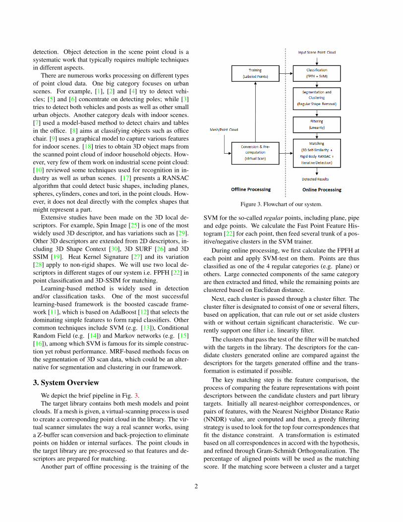
3. System OverviewWe depict the brief pipeline in Fig. 3.The target library contains both mesh models and point

clouds. If a mesh is given, a virtual-scanning process is usedto create a corresponding point cloud in the library. The vir-tual scanner simulates the way a real scanner works, usinga Z-buffer scan conversion and back-projection to eliminatepoints on hidden or internal surfaces. The point clouds inthe target library are pre-processed so that features and de-scriptors are prepared for matching.

Another part of offline processing is the training of the

Figure 3. Flowchart of our system.

SVM for the so-called regular points, including plane, pipeand edge points. We calculate the Fast Point Feature His-togram [22] for each point, then feed several trunk of a pos-itive/negative clusters in the SVM trainer.

During online processing, we first calculate the FPFH ateach point and apply SVM-test on them. Points are thusclassified as one of the 4 regular categories (e.g. plane) orothers. Large connected components of the same categoryare then extracted and fitted, while the remaining points areclustered based on Euclidean distance.

Next, each cluster is passed through a cluster filter. Thecluster filter is designated to consist of one or several filters,based on application, that can rule out or set aside clusterswith or without certain significant characteristic. We cur-rently support one filter i.e. linearity filter.

The clusters that pass the test of the filter will be matchedwith the targets in the library. The descriptors for the can-didate clusters generated online are compared against thedescriptors for the targets generated offline and the trans-formation is estimated if possible.

The key matching step is the feature comparison, theprocess of comparing the feature representations with pointdescriptors between the candidate clusters and part librarytargets. Initially all nearest-neighbor correspondences, orpairs of features, with the Nearest Neighbor Distance Ratio(NNDR) value, are computed and then, a greedy filteringstrategy is used to look for the top four correspondences thatfit the distance constraint. A transformation is estimatedbased on all correspondences in accord with the hypothesis,and refined through Gram-Schmidt Orthogonalization. Thepercentage of aligned points will be used as the matchingscore. If the matching score between a cluster and a target

2

Figure 4. Illustration of Point Feature Histogram calculation.

is higher than some threshold, the cluster is considered tobe a detected instance of the target.

In case that there are multiple targets in a single clus-ter, we iteratively remove the aligned part and check theremaining part of the cluster until it’s small enough.

4. SVM-based Point ClassificationWe initially observed that, in our data set of large outdoor

industrial scene, a large portion of the points belong to basicgeometrical shapes, mainly planes (e.g. ground, ladders andboxes) and pipe-shapes (cylindrical pipes, bent connection,posts). Therefore, removing large clusters of such pointswill largely ease and accelerate our processing and help usfocus on interested objects that we would like to detect.

4.1. Fast Point Feature Histogram

We select the 33-dimensional Fast Point Feature His-togram (FPFH) as our descriptor. The reason for selectingFPFH could be found in Section 8.1.

FPFH is an approximate and accelerated version of PointFeature Histogram (PFH) [21]. PFH uses a histogram to en-code the geometrical properties of a point’s neighborhoodby generalizing the mean curvature around the point. Thehistogram representation is quantized based on all relation-ships between the points and their estimated surface nor-mals within the neighborhood (Fig. 4).

The local frame for computing the relative difference be-tween two points ps and pt is defined in Equation 1.

u = ns

v = u× (pt − ps)

∥pt − ps∥2w = u× v

(1)

With this frame, the difference between the point-normalpair can be represented by the following angles (Equ. 2):

α = v · nt

ϕ = u · (pt − ps)

∥pt − ps∥2θ = arctan(w · nt, u · nt)

(2)

These angles are then quantized to form the histogram.

FPFH [22] reduces the computational complexity ofPFH from O(nk2) to O(nk), where k is the number ofneighbors for each point p in point cloud P, without losingmuch of the discriminative power in PFH:

FPFH(pq) = PFH(pq) +1

k

k∑i=1

1

wk· PFH(pk). (3)

In our experiment, we use the version implemented inthe open-source Point Cloud Library (PCL) [23].

4.2. Classification by SVM

In the offline training stage, We manually select and labelabout 75 representative small trunks of point cloud, addingup to around 200k labeled points.

For support vector machine, we use LIBSVM package[31] with radial basis function (RBF) as kernel, in whichparameters C = 8 and γ = 0.5. Details of SVM could befound in [31] and here we focus on the selection of trainingdata that determines the property of the classifier.

4.3. More Regular Classes: Edge and Thin Pipe

During experiments, we found that near places wheretwo or more planes intersect, some points would not be clas-sified as plane point due to the interference of another planein their neighborhood. On the other hand, these points ob-viously do not belong to parts when they group together asa large cluster. Therefore, we assign them to another cate-gory, namely the Edge.

Besides edges, we also found some thin pipes missing inpipe detection. Experiments show that simply adding themin the training dataset might have negative effects on pipeswith larger sizes, which suggests that they may need to beregarded as a separate category from pipes (partially due tothe neighborhood size of the FPFH descriptor).

To judge the generalization ability, or distinctiveness ofpipes in different sizes, we perform a series of cross valida-tion, summarized in Table 1. We can see that the 10/15/20-cm pipe classifiers could classify the 10/15/20-cm pipes in-terchangeably, while 5-cm pipe classifier will distinguishthe 5-cm pipe from the others. This evidence also offerssupport to separate the category Thin-Pipe from the cate-gory Pipe. If we need to distinguish between 10/15/20-cmpipes, however, we may add the other sizes as negative ex-amples to get more precise boundaries between them.

We perform SVM 4 times, once for each category. Pointsare thus labeled as plane, pipe, edge, thin-pipe or others.Figure 5 shows the classified pipe points and plane points.Note that, some pipe-shaped objects e.g. tanks are so hugethat locally they are like planes. In our experiments, wefound it better for segmentation if we label the large tankswith small curvature as planes rather than cylinders.

3

Training/Testing 5 cm 10 cm 15 cm 20 cm5 cm Y N N N10 cm N Y Y Y15 cm N Y Y Y20 cm N Y Y Y

Table 1. Cross validation result for pipes of different sizes. The leftcolumn means the training data, and the top row means the testingdata. Y means at least 80% of the testing points are classified aspipe, while N means the opposite.

Figure 5. Classification result of pipe points (in green), planepoints (in yellow), edge points (in blue), thin-pipe points (in darkgreen) and the others (in red).

5. Segmentation and ClusteringThere are many segmentation methods, e.g. the min-

cut [34] approach and other approaches derived from 2Dcases. However, since we have made quite confident classi-fication of non-part (background) points, the segmentationtask could be done in a fast and light-weighted manner.

We iteratively select a random unvisited seed point andexpand it to unvisited neighboring points within a givenEuclidean distance using the classical Flood-Fill algorithm.The neighbor threshold is determined by the granularity ofthe input cloud. Apparently after finite steps the residualcloud will be divided into a number of disjoint clusters.

We apply the clustering routine for five times. First wedo clustering on points labeled as one of the four categoriesand get a list of plane/pipe/edge/thin-pipe clusters, respec-tively. Then we subtract the big clusters from the orig-inal point cloud. This is important since we don’t wantto remove small area of regular shapes that might lie on abig part. Finally, clustering is performed on the remainingpoints that we believe to be part points.

Using S(C) to denote the set of points in category C, thealgorithm could be written as:

S(Candidate) :=S(All)− S(Plane)− S(Pipe)

− S(Edge)− S(ThinPipe).(4)

Finally, we can formally make an extendable definitionof the candidates by Equ. 5:

Figure 6. Segmentation result of the remaining candidate points.

S(Candidate) := S(Irregular)

= S(All)−∪i

S(Regulari),(5)

where Regulari can be any connected component withrepetitive patterns and large size. This definition also offersus the possibility of discovering candidates of new targetsthat are actually not in the database.

Figure 6 shows the segmentation and clustering resultfrom the previous steps.

6. Cluster FilterWe observed that not all clusters are worth doing the de-

tailed matching. In fact, most clusters in a scene will notbe what we are interested in even at first glance. Therefore,we first pass the clusters through filters that can quickly ruleout or set aside clusters with or without certain characteris-tic. The filters should be extremely fast while able to filterout quite a number of impossible candidates. Currently wehave implemented a linearity filter.

The linearity of a cluster is evaluated by the absolutevalue of the correlation coefficient in the Least Squares Fit-ting on the 2D points of the three projections on the x − y,y − z and z − x planes. For example,

rxy =

∑ni=1 (xi − x)(yi − y)√∑n

i=1 (xi − x)2 ∗∑n

i=1 (yi − y)2, (6)

and the linearity score is measured by Equation 7:

r = max(|rxy|, |ryz|, |rzx|). (7)

The cluster would be considered to be linear if r > 0.9,meaning that at least one of its projections could be fittedby a line with high confidence. Note that planes and thin-pipes may fall in this linear category, but since both of themare supposed to be removed in the classification step, anyremaining linear clusters are considered as lines, missedpipes, missed planes or noise. Experiments show that thelinearity scores of all representative targets are below 0.8,with a substantial margin from the threshold of 0.9, mean-ing that our target objects won’t be filtered out in this step.

4

In one of our experiments, only 1491 candidates are remain-ing, out of 1905 initial clusters from previous steps, afterruling out the most linear clusters.

7. Matching based on 3D SSIM Descriptor7.1. Feature and Descriptor Generation

We follow the method in [19] to match between the can-didate and the target point clouds. However, we use a sim-plified version i.e. the normal similarity since there’s typi-cally no intensity information in the targets.

The feature extraction process is performed such that 3Dpeaks of local maxima of principle curvature are detected inspatial-space. Given an interest point and its local region,there are two major steps to construct the descriptor.

Firstly, the 3D extension of the 2D self-similarity surfacedescribed in [20], is generated using the normal similarityacross the local region. The normal similarity between twopoints x and y is defined by the angle between the normals,as Equ. 8 suggests (Assume ||n(·)|| = 1).

s(x, y, fn) = [π − cos−1(fn(x) · fn(y))]/π= [π − cos−1(n(x) · n(y))]/π.

(8)

Note that when the angle is 0, the function returns 1;whereas the angle is π, i.e. the normals are opposite to eachother, the function returns 0.

Then, the self-similarity surface is quantized along log-spherical coordinates to form the 3D self-similarity descrip-tor in a rotation-invariant manner. This is achieved by usinglocal reference system at each key point: the z-axis is the di-rection of the normal; the x-axis is the direction of the prin-cipal curvature; and the y-axis is the cross product of z andx directions. In this application we set 5 divisions in radius,longitude and latitude, respectively, and replace the valuesin each cell with the average similarity value of all points inthe cell, resulting in a descriptor of 5× 5× 5 = 125 dimen-sions. The dimension is greatly reduced without deductionof performance, which is another important difference from[19]. Finally, the descriptor is normalized by scaling thedimensions with the maximum value to be 1.

7.2. Matching

Our detection is based on matching, during which thedescriptors for the candidate clusters generated online arecompared against the descriptors for the targets generatedoffline and the transformation is estimated.

To establish the transformation, it’s natural to first calcu-late the nearest-neighbor correspondences with any NearestNeighbor Distance Ratio (NNDR) (introduced in [24]) be-tween the candidate cluster and the target from the library.Then, unlike the normal RANSAC procedure, we propose a

greedy algorithm based on the observation that (1) the top-ranked correspondences are more likely to be correct; (2)the objects we are detecting are rigid industrial parts withfixed standard size and shapes. In general, the transforma-tion can be represented as Equ. 9:

p′ = sRp+ T. (9)

where s is the scaling factor, R is the rotation matrix andT is the translation vector. For rigid-body transformation,s = 1, so we need to solve for the 12 unknowns in 3 ×3 matrix R and 3 × 1 vector T , which requires at most 4correspondences of (p, p′) here. (Note, however, that thereare only 7 independent variables.)

We propose a greedy 4-round strategy to find the 4 cor-respondences based on the following insight: rigid-bodytransformation preserves the distance between the points.

Initially we have all nearest-neighbor correspondenceswith any NNDR value in the candidate set; In the beginningof round i, the correspondence with the minimum NNDRvalue, ci = (ai, bi), is added to the final correspondenceset and removed from the candidate set. Then, for each ofthe correspondence c′ = (a′, b′) in the candidate set, cal-culate the Euclidean distance dist(a′, ai) and dist(b′, bi),and if the ratio of the (squared) distance is larger than somethreshold (1.1), c′ will be removed from the candidate set.

If the candidate set becomes empty within 4 rounds, wewill discard the match as a failed rigid-body match; other-wise the transformation could be estimated over at least 4distance-compatible correspondences. Specifically, a 3× 3affine transformation matrix and a 3D translation vector issolved from the equations formed by the correspondences.

To prevent matching from being sensitive to the first cor-respondence, multiple initial seeds are tried and only thetransformation with the highest alignment score is selected.Finally, the rigid-body constraint is used again to refine theresult, through the Gram-Schmidt Orthogonalization of thebase vectors (R = (u1, u2, u3)):

u′1 = u1

u′2 = u2 − proj u′

1(u2)

u′3 = u3 − proj u′

1(u3)− proj u′

2(u3)

(10)

which are then normalized using:

e′i =u′i

∥u′i∥

(i = 1, 2, 3). (11)

A point p in cluster A is said to be aligned with cluster Bif the nearest neighbor in cluster B to p under the transfor-mation is within some threshold (5e-4 for industrial scene).The alignment score is thus defined as the percentage ofaligned points. If the alignment score between a cluster anda target is larger than 0.6, the cluster is considered to be adetected instance of the target.

5

Figure 7. Parts detection in an assembly.

7.3. Iterative Detection

In case that there are multiple targets in a single clus-ter, we iteratively remove the aligned part through the cloudsubtraction routine, and examine the remaining part of thecluster until it’s too small to be matched.

Here is a demonstration of our algorithm against multi-target detection in a single cluster. We cut an assembly intoseveral parts and use them as query. They were detectedone-by-one through our alignment and iterative detectionprocess (Fig. 7). Note that no segmentation is involved, andthe descriptors are not identical at the same location of thepart and the assembly.

8. Discussion8.1. Choice of Descriptor for Classification

The principle for the selection of descriptor for classifi-cation can be depicted as: everything should be as simpleas possible, but not simpler. This is because we aim at clas-sifying basic geometric shapes. By simple we mean thatthe calculation is not expensive, and the dimension is small.One of the simplest features is Shape Index [33], however, itonly considers the principal curvatures, which is not distinc-tive enough for multiple categories in our case. On the otherhand, brief experiments on simple shape classification showthat other descriptors such as Spin Image [25] and 3D ShapeContext [30] are outperformed by FPFH [22] in both accu-racy and efficiency. Note that, however, the performance ofthe descriptors could be quite different when they are usedin, for example, complex shape matching.

8.2. Choice of Learning Method

As mentioned in Section 2, there are many learningmethods available. We choose SVM as our classifier basedon the following reasons: Firstly, we only aim at classifyingsimple geometric shapes, thus we need neither too compli-cated descriptors nor too complicated classifiers; secondly,we need the generalization ability from the classifier sincewe only have a limit number of training examples (espe-cially for the parts) while there might be many more typesof shapes; finally, although there can be as many as 5 cate-gories, they are not equivalent because Part is the only cat-

Classifier #TrC #TrP #SVPlane 14/23 94602 2069/2063Pipe 14/9 91613 1496/1503Edge 9/24 94838 1079/1121

Thin Pipe 8/22 83742 1020/1035

Table 2. Classifiers. TrC = Training Cluster, TrP = Training Point,SV = Support Vector. The ratio means Positive/Negative.

Original Plane Pipe Edge Thinpipe#Pts 25,135k 14,137k 8,767k 6,015k 5,534k(%) 100.0% 56.2% 34.9% 23.9% 22.0%

Table 3. Remaining points after removal of each point category.

egory that will be used in detection, thus we propose a sub-traction process over the 2-class classification results (Equ.4, 5). We do want to consider the scalability when we try toapply SVM to more complicated multi-class objects in thefuture, however, since we don’t care much now about theboundaries between categories other than the parts (e.g. bigpipes can be classified as plane, pipes can be classified asthin pipes as long as the result is consistent), the algorithmis efficient enough to solve the seemingly multi-class, butintrinsically 2-class problem.

9. Experiment Results9.1. SVM Classifier Training

Generally speaking we have five categories of the train-ing clusters: Plane, Pipe, Edge, Thin-Pipe and Part. Sincewe are using two-class classification, when we are train-ing one kind of classifier, all clusters labeled as this classwill be regarded as the positive example, while the nega-tive samples will be selected from the remaining categories.We summarize the statistics of training data in Table 2. Thenumber of support vectors shows the complexity of the cat-egory, in order to distinguish it from the others. Table 3shows the number of points in the residual point cloud af-ter removing each of the four categories. Nearly half of thepoints are classified as plane, while after removing pipesthere are one third of points, and finally only one fifth of theoriginal points need to be considered in detection, whichshows the effectiveness of the point classification step.

9.2. Ground Lidar

In this section, we show the testing results of our methodon the industrial scene point cloud.

A result for the sub-scene is shown in Figure 8, where de-tected parts are highlighted with colors and bounding boxes.Figure 9 shows another result with respect to ground truth:the red color means false negative i.e. the object is missdetected or the point on the candidate cluster is misaligned;the blue color means false positive i.e. there is no target at

6

Figure 8. Detected parts, including handles, valves, junctions andflanges.

Figure 9. Detected parts on top of the tanks.

Category #Sub-cat. #Truth #TP #FP #FNBall 1 22 11 4 11

Connection 2 3 0 0 3Flange 4 32 20 3 12Handle 6 10 3 1 7

Spotlight 1 6 1 0 5Tanktop 2 4 3 3 1

T-Junction 5 25 7 0 18Valve 12 25 17 24 8All 33 127 62 35 65

Table 4. Statistics of detection. There are 8 big categories, 33sub-categories and 127 instances (Ground-truth) of targets in thescene. Among them 62 are correctly identified (TP = True Posi-tive), while 35 detections are wrong (FP = False Positive), and 65instances are missed (FN = False Negative).

the position but the algorithm detected one, or the point onthe target is misaligned. Yellow/cyan both mean true posi-tive i.e. the aligned points are close enough.

Table 4 and Fig. 10 show the statistical results of the in-dustrial scene. Balls, flanges, tanktops and valves are moresuccessfully detected than the other objects.

9.3. Publicly Available Data

The experiment results show that our method works withthe virtual point clouds almost as well as with the real pointclouds. Since the virtual point clouds could be automat-

Figure 10. Precision-recall curve of the industrial part detection.

(a) (b)

Figure 11. Detection and alignment result from the cluttered scene.The chef is detected twice from two different sub-parts.

ically generated from mesh models with the virtual scan-ner, we can expect the fully-automatic matching betweenthe point clouds and the mesh models.

To compare our method with the other methods, we havealso tested our algorithm on some of the following publiclyavailable data. Figure 11 shows one detection result of thecluttered scene [32]. Note that only one face is present inthe scene point cloud, and occlusions lead to discontinu-ity of some parts, which make the data quite challenging.Moreover, our point classification phase does not contributeto the result in this case.

10. Conclusion

In this paper, we present an object detection frame-work for 3D scene point cloud, using a combinationalapproach containing SVM-based point classification, seg-mentation, clustering, filtering, 3D self-similarity descrip-tor and rigid-body RANSAC. The SVM+FPFH method inpipe/plane/edge point classification gives a nice illustrationof how descriptor could be combined with training meth-ods. Applying two local descriptors (FPFH and 3D-SSIM)in different phases of processing shows that different de-scriptors could be superior under different circumstances.The proposed variant of RANSAC considering the rigidbody constraint also shows how prior knowledge could beincorporated in the system. The experiment results showthe effectiveness of our method, especially for large clut-tered industrial scenes.

7

AcknowledgementThis research was supported by CiSoft project sponsored

by Chevron. We appreciate the management of Chevron forthe permission to present this work.

References[1] A. Patterson, P. Mordohai and K. Daniilidis. Object Detec-

tion from Large-Scale 3D Datasets using Bottom-up and Top-down Descriptors. ECCV 2008. 2

[2] A. Frome, D. Huber, R. Kolluri, T. Bulow, and J. Malik. Rec-ognizing Objects in Range Data Using Regional Point De-scriptors. ECCV 2004. 2

[3] A. Golovinskiy, V. G. Kim, T. Funkhouser. Shape-basedRecognition of 3D Point Clouds in Urban Environments.ICCV 2009. 2

[4] Rapid Object Indexing Using Locality Sensitive Hashing andJoint 3D-Signature Space Estimation. PAMI 2006. 2

[5] H. Yokoyama, H. Date, S. Kanai and H. Takeda. Detection andClassification of Pole-like Objects from Mobile Laser Scan-ning Data of Urban Environments. ACDDE 2012. 2

[6] M. Lehtomaki, A. Jaakkola, J. Hyyppa, A. Kukko, H. Kaarti-nen. Detection of Vertical Pole-Like Objects in a Road Envi-ronment Using Vehicle-Based Laser Scanning Data. RemoteSensing 2010. 2

[7] B. Steder, G. Grisetti, M. V. Loock and W. Burgard. RobustOn-line Model-based Object Detection from Range Images.IROS 2009. 2

[8] A. Nuchter, H. Surmann, J. Hertzberg. Automatic Classifica-tion of Objects in 3D Laser Range Scans. IAS 2004. 2

[9] H. Koppula, A. Anand, T. Joachims and A. Saxena. SemanticLabeling of 3D Point Clouds for Indoor Scenes. NIPS 2011.2

[10] G. Vosselman, B. Gorte, G. Sithole, T. Rabbani. RecognisingStructure in Laser Scanner Point Clouds. IAPRS 2004. 2

[11] P. Viola and M. Jones. Rapid object detection using a boostedcascade of simple features. In Proc. CVPR 2001. 2

[12] Y. Freund and R. Schapire. A Decision-Theoretic Gener-alization of On-line Learning and an Application to Boost-ing. Journal of Computer and System Sciences, 55(1):119-139, August 1997. 2

[13] M. Himmelsbach, A. Muller, T. Luttel and H.-J. WunscheLIDAR-based 3D Object Perception IWCTS 2008. 2

[14] X. Xiong, D. Huber. Using Context to Create Semantic 3DModels of Indoor Environments BMVC 2010. 2

[15] D. Anguelov, B. Taskar, V. Chatalbashev, D. Koller, D.Gupta, G. Heitz, A. Ng. Discriminative Learning of MarkovRandom Fields for Segmentation of 3D Scan Data. In:IEEE Conference on Computer Vision and Pattern Recogni-tion (CVPR) 2005, IEEE Computer Society, pp 169-176. 2

[16] R. Shapovalov, A. Velizhev. Cutting-Plane Training of Non-associative Markov Network for 3D Point Cloud Segmenta-tion. 3DIMPVT 2011. 2

[17] R. Schnabel, R. Wahl, and R. Klein. Efficient RANSAC forPoint-Cloud Shape Detection Computer Graphics Forum, vol.26, no. 2, pp. 214-226, June 2007. 2

[18] R. B. Rusu, Z. C. Marton, N. Blodow, M. Dolha, and M.Beetz. Towards 3D Point Cloud Based Object Maps forHousehold environments. Robotics and Autonomous SystemsJournal (Special Issue on Semantic Knowledge), 2008. 2

[19] J. Huang, and S. You. Point Cloud Matching based on 3DSelf-Similarity International Workshop on Point Cloud Pro-cessing (Affiliated with CVPR 2012), Providence, Rhode Is-land, June 16, 2012. 2, 5

[20] E. Shechtman and M. Irani. Matching Local Self-Similaritiesacross Images and Videos. In Proc. CVPR, 2007. 5

[21] R. B. Rusu, Z. C. Marton, N. Blodow, and M. Beetz. Per-sistent Point Feature Histograms for 3D Point Clouds. In Pro-ceedings of the 10th International Conference on IntelligentAutonomous Systems, 2008. 3

[22] R. B. Rusu, N. Blodow, and M. Beetz. Fast Point FeatureHistograms (FPFH) for 3D Registration in Proceedings of theIEEE International Conference on Robotics and Automation(ICRA), Kobe, Japan, May 12-17 2009. 1, 2, 3, 6

[23] R. B. Rusu and S. Cousins. 3D is here: Point Cloud Library(PCL). In Proceedings of the IEEE International Conferenceon Robotics and Automation (ICRA ’11), Shanghai, China,May 2011. 3

[24] K. Mikolajczyk and C. Schmid. A Performance Evaluationof Local Descriptors. IEEE Transactions on Pattern Analysisand Machine Intelligence, vol. 27, no. 10, pp. 1615-1630, Oct.2005. 5

[25] A. Johnson and M. Hebert. Object recognition by Match-ing Oriented Points. In Proceedings of the Conference onComputer Vision and Pattern Recognition, Puerto Rico, USA,pages 684.689, 1997. ICCV 1997. 2, 6

[26] J. Knopp, M. Prasad, G. Willems, R. Timofte, and L. VanGool. Hough Transform and 3D SURF for Robust Three Di-mensional Classification. In: ECCV. 2010. 2

[27] J. Sun, M. Ovsjanikov, and L. Guibas. A Concise and Prov-ably Informative Multi-scale Signature based on Heat Diffu-sion. In: SGP. 2009 2

[28] M. M. Bronstein and I. Kokkinos. Scale-Invariant Heat Ker-nel Signatures for Non-rigid Shape Recognition. In Proc.CVPR 2010. 2

[29] S. Ruiz-Correa, L. G. Shapiro, and M. Melia. A NewSignature-based Method for Efficient 3-D Object Recogni-tion. In Proc. CVPR, 2001. 2

[30] M. Kortgen, G.-J. Park, M. Novotni, and R. Klein. 3D shapematching with 3D Shape Contexts. In The 7th Central Euro-pean Seminar on Computer Graphics, April 2003. 2, 6

[31] C.-C. Chang and C.-J. Lin. LIBSVM: A Library for Sup-port Vector Machines. (2011) [Online]. Available: http://www.csie.ntu.edu.tw/˜cjlin/libsvm 3

[32] Ajmal Mian, M. Bennamoun and R. Owens. 3D Model-based Object Recognition and Segmentation in ClutteredScenes. IEEE Trans. on Pattern Analysis and Machine In-telligence (PAMI), vol. 28(10), pp. 1584–1601, 2006. 7

[33] J. J. Koenderink. Solid Shape. MIT Press, 1990. 6[34] A. Golovinskiy and T. Funkhouser. Min-cut based Segmen-

tation of Point Clouds. in IEEE Workshop on Search in 3Dand Video (S3DV) at ICCV, Sept. 2009. 4

8