Embed Size (px)
Citation preview

DESIGN OF RECYCLE/REUSE NETWORKS WITH THERMAL
EFFECTS AND VARIABLE SOURCES
A Thesis
by
JOSE GUADALUPE ZAVALA OSEGUERA
Submitted to the Office of Graduate Studies of Texas A&M University
in partial fulfillment of the requirements for the degree of
MASTER OF SCIENCE
August 2009
Major Subject: Chemical Engineering

DESIGN OF RECYCLE/REUSE NETWORKS WITH THERMAL
EFFECTS AND VARIABLE SOURCES
A Thesis
by
JOSE GUADALUPE ZAVALA OSEGUERA
Submitted to the Office of Graduate Studies of Texas A&M University
in partial fulfillment of the requirements of the degree of
MASTER OF SCIENCE
Approved by:
Chair of Committee, Mahmoud M. El-Halwagi Committee Members, M. Sam Mannan Sergiy Butenko Head of Department, Michael V. Pishko
August 2009
Major Subject: Chemical Engineering

iii
ABSTRACT
Design of Recycle/Reuse Networks with Thermal Effects and Variable Sources.
(August 2009)
Jose Guadalupe Zavala Oseguera,
B. Eng. University of Guanajuato, Mexico;
M. Eng. University of Guanajuato, Mexico
Chair of Advisory Committee: Dr. Mahmoud El-Halwagi
Recycle/reuse networks are commonly used in industrial facilities to conserve
natural resources, reduce environmental impact, and improve process economics. The
design of these networks is a challenging task because of the numerous poss ibilities of
assigning stream (process sources) to units that may potentially employ them (process
sinks). Additionally, several fresh streams with different qualities and costs may be used
to supplement the recycle of process streams. The selection of the type and flow of these
fresh resources is an important step in the design of the recycle/reuse networks. This
work introduces systematic approaches to address two new categories in the design of
recycle/reuse networks:
(a) The incorporation of thermal effects in the network. Two new aspects are
introduced: heat of mixing of process sources and temperature constraints imposed on
the feed to the process sinks

iv
(b) Dealing with variation in process sources. Two types of source variability
are addressed: flowrate and composition
For networks with thermal effects, an assignment optimization formulation is
developed. Depending on the functional form of the heat of mixing, the formulation may
be a linear or a nonlinear program. The solution of this program provides optimum
flowrates of the fresh streams as well as the segregation, mixing, and allocation of the
process sources to sinks. For networks with variable sources, a computer code is
developed to solve the problem. It is based on discretizing the search space and using the
concept of “floating pinch” to insure solution feasibility and optimal targets. Case
studies are solved to illustrate the applicability of the new approaches.

v
DEDICATION
To my beloved son: Alex.

vi
ACKNOWLEDGEMENTS
I want to acknowledge their support to all of those who where helping me in this
marvelous stage of my life. In this way, first I would like to acknowledge my advisor
because of his net style of lifelong leadership and dedication. Also, I want to say thanks
to my family and friends for their support during the difficulties, and to my classmates
for sharing this experience with me. At the same time, is not possible to found the
correct phase to express all my gratitude to Texas A&M University for giving me the
opportunity to continue my studies in such a great environment. In the same way, I wish
to express my most sincere gratitude to the people of the great state of Texas and thanks
to God for his forgiveness, for his help, and for his love.

vii
NOMENCLATURE
CFresh = cost of the fresh resource ($/kg)
Gj = flowrate demand for sink j (tons/hr)
Nsinks = number of sinks
Nsources = number of sources
Ti = temperature of source i (K)
waste = total amount of flow going to waste (kg/hr)
Wi = flow rate of source i (kg/hr)
jiw , = amount of flow from source i to sink j (kg/hr)
in
kiy , = composition kth component of source i (ppm)
min
,kjz = lower bound for kth-component composition to sink j (ppm)
z in
kj, = inlet composition for kth-component composition to sink j (ppm)
max
,kjz = upper bound for kth-component composition to sink j(ppm)
Indices
i = sources
j = sinks
k = component
u = interceptor

viii
TABLE OF CONTENTS
Page
ABSTRACT ......................................................................................................... iii
DEDICATION ..................................................................................................... v
AKNOWLEDGEMENTS .................................................................................... vi
NOMENCLATURE ............................................................................................. vii
TABLE OF CONTENTS ..................................................................................... viii
LIST OF FIGURES .............................................................................................. x
LIST OF TABLES ............................................................................................... xi
CHAPTER
I INTRODUCTION: DESIGN OF RECYCLE/REUSE
NETWORKS WITH THERMAL EFFECTS AND VARIABLE
SOURCES........................................................................................ 1
II LITERATURE REVIEW ................................................................ 4
III PROBLEM STATEMENT .............................................................. 7
III.1 Networks with thermal effects .............................................. 7 III.2 Networks with variable sources ............................................ 8 III.3 Design challenges.................................................................. 9
IV OPTIMIZATION APPROACH FOR DESIGN OF RECYCLE/
REUSE NETWORKS WITH THERMAL EFFECTS .................... 10
IV.1 Problem representation.......................................................... 10 IV.2 Mathematical formulation ..................................................... 11 IV.3 Case study: reduction of acetic acid usage in a vinyl acetate monomer plant .......................................................... 14

ix
CHAPTER Page
V DIRECT RECYCLE WITH VARIABLE SOURCES .................... 18 V.1 Problem scope ....................................................................... 18 V.2 Basics of the floating pinch concept ..................................... 18 V.3 Computer-aided approach for the floating pinch implementation in recycle/reuse targeting ............................ 23 V.4 Iterative procedure for global solution .................................. 31 V.5 Acetic acid case study ........................................................... 33 V.6 Water recycle example .......................................................... 34
VI CONCLUSIONS AND RECOMMENDATIONS .......................... 39
VI.1 Conclusions ........................................................................... 39 VI.2 Recommendations for future work........................................ 40
REFERENCES ..................................................................................................... 42
APPENDIX A ...................................................................................................... 45
VITA…………..................................................................................................... 61

x
LIST OF FIGURES
FIGURE Page
4.1 Direct recycle problem representation ............................................. 11
4.2a Direct recycle configurations: without thermal effects.................... 16
4.2b Direct recycle configurations: with temperature constraints for the sinks ................................................................................................. 16
4.2c Direct recycle configurations: with temperature constraints with heat of mixing considerations .......................................................... 17
5.1 Direct recycle and heat integration pinch location........................... 19
5.2 Schematic representation of the floating pinch concept .................. 20
5.3 Source-sink composite diagram to define load intervals ................. 22
5.4 Structure of the generic LINGO model for the direct recycle/reuse case study ......................................................................................... 27
5.5 Flowchart for pinch candidate analysis and source-sink balances... 32
5.6 Direct recycle configuration results for the acetic acid case study .. 33
5.7 Pinch location for the variable flow case study with a flowrate of 120 tonnes/h and concentration of 100 ppm for source 1 ................ 38
6.1 Simultaneous synthesis for direct recycle/reuse (DRR), heat exchange networks (HEN) and mass exchange networks (MEN) ... 40

xi
LIST OF TABLES
TABLE Page
4.1 Source data for the vinyl acetate example ....................................... 14
4.2 Sink data for the vinyl acetate example ........................................... 15
5.1 Sink data for the water reuse example ............................................. 34
5.2 Source data for the water reuse example ......................................... 35
5.3 Results with the modular approach for direct recycle integration ... 36

1
CHAPTER I
INTRODUCTION: DESIGN OF RECYCLE/REUSE NETWORKS WITH
THERMAL EFFECTS AND VARIABLE SOURCES
Process Integration (PI) is an effective framework for continuous improvement in
the performance of industrial processes. One category of improvements focuses on the
structural configuration of the chemical processes in a comprehensive context. Several
categories of structural improvements have already been addressed in literature and
associated methodologies have been developed. Of particular interest in the structural
modification geared towards recovering materials via recycle/reuse approaches. Material
recycle/reuse is a primary industrial strategy for conserving natural resources, reducing
operating costs, and mitigating the negative environmental impact. The direct
recycle/reuse is one category of the general recycle/reuse network. The objective of this
problem is to identify cost-effective allocation of process streams (sources) to process
units (sinks) without adding new equipment to the process. Examples of sources in direct
recycle/reuse systems are the waste or low value streams considered for recycling.
Examples of sinks are those units to which such streams may be recycled.
____________ This thesis follows the style of Computers and Chemical Engineering.

2
In addressing recycle/reuse, various objectives may be used. These include cost,
flowrates of fresh resources, and flowrates and loads of discharge wastes. Other
important metrics include operability, reliability, and safety. It is also possible to
establish trade-offs among these objective functions. These objective functions are
subject to a variety of constraints. Direct recycle/reuse will search for the appropriate
stream allocation without violating the process specification and constraints.
One of the hallmarks of process integration is to use systematic procedures to find
solutions. It is important here to identify properly the type of method which should be
applied for each application. Sometimes, structural representation approaches are used to
determine the exact configuration of the solutions. In other cases, approaches are used to
determine performance targets which can be determined ahead of detailed design. In
this regard, the “pinch” technology is quite effective. Performance targets in terms of
minimum amount of fresh requirements and waste flow are necessary for direct
recycle/reuse integration. These targets are very important in benchmarking the
performance of the recycle/reuse network.
It is worth noting that several systematic procedures to design material recovery
networks have been proposed. These procedures include the allocation or reuse of
materials in process units through graphic, algebraic, and optimization methods as will
be described in Chapter II of this work. In many cases, constraints on process sinks are
not limited to purity (or concentration of certain components). Instead, there is typically
a combination of composition and temperature constraints. Therefore, the design of
recycle/reuse network must include the consideration of both composition and

3
temperature. Chapter III describes the problem statement which addresses two new
classes of recycle/reuse networks: thermal effects for source mixing and sink constraints
and variation in flowrate and composition of the sources. Chapters IV and V present the
proposed solution procedures, mathematical formulations, and case studies. Chapter VI
discusses the conclusions of this thesis and recommendations for future work.

4
CHAPTER II
LITERATURE REVIEW
Material recycle/reuse has received much research attention. Recycle corresponds
to the utilization of a process stream (e.g., a waste or a low-value stream) in a process
unit (a sink). On the other hand, reuse refers to the reapplication of the stream for the
original intent or in the original unit. Ensuring optimum recycle/reuse of process streams
is among the key objectives of processing facilities. Therefore, it is important to develop
systematic procedures to design the material recovery networks and to assign the
recovered materials to proper process units. Several research efforts have endeavored to
address the problem of designing recycle/reuse systems. These efforts include graphical,
algebraic, and optimization approaches.
Several graphical approaches have been devised to minimize wastewater discharge
by fostering recycle/reuse of process water streams. Wang and Smith (1994) developed a
pinch-based visualization technique to minimize fresh water consumption and
wastewater discharged while transferring contaminants from process streams to water
streams in units that function as mass exchangers. This approach is an extension of the
mass-exchange network problem introduced by El-Halwagi and Manousiouthakis (1989)
and is based on modeling water-using units as mass exchangers. Dhole et al. (1996) and
El-Halwagi and Spriggs (1996) noted that there are various water units that may not be
treated as mass exchangers. They explain the problem of material usage and discharge
as a source-sink mapping task. According to their study, each process has a number of

5
sources (streams available for recycle/reuse) that may be allocated to sinks (units that
demand certain feeds and may accept the recycled sources). Fresh resources (e.g., fresh
water, solvents, material utilities) may be used to supplement the use of process sources
so as to meet the sink demands at minimum cost. Dhole et al. (1996) developed a
graphical representation of concentration versus flowrate. Composite curves for supply
and demand are overlapped until a pinch point is created. El-Halwagi and Spriggs (1996)
developed a source-sink mapping representation and used lever-arm rules to identify
optimum allocation of sources to sinks. Polley and Polley (2000) outlined optimality
conditions for sequencing recycles. El-Halwagi et al. (2003) developed a material
recovery pinch analysis that rigorously identifies minimum fresh usage, maximum
recycle, and minimum waste discharge.
Algebraic techniques have also been developed to address recycle/reuse problems.
Sorin and Bedard (1999) introduced an evolutionary technique based on mixing source
streams at concentrations bordering the demand location and moving on progressively to
higher concentration. This approach may become tedious for systems involving many
sources and sinks. Hallale (2002), Alves and Towler (2002), and Alves (1999) developed
a surplus diagram for the recycle of species such as water and hydrogen. This approach
involves extensive computations to reconcile flowrate and purity requirements. Manan et
al. (2004) refined the surplus approach by developing a cascade approach to avoid the
extensive calculations in identifying the targets.
Takama et al. (1980) developed an optimization-based approach to recycle water.
This approach has been generalized later by several researchers (e.g., Alva-Argaez et al.,

6
1999; Keckler and Allen, 1999; Benko et al., 2000; Savelski and Bagajewicz, 2000,
2001; and Dunn et al., 2001).
The aforementioned research efforts have been limited to direct recycle/reuse
strategies in which sources are directly assigned to sinks. No new equipment is added.
To overcome this limitation, Gabriel and El-Halwagi (2005) developed an optimization
approach which includes interception devices in addition to sources and sinks. The
interception devices are new equipment that are added to the process in order to adjust
the purity of the various sources prior to recycle/reuse.

7
CHAPTER III
PROBLEM STATEMENT
Two new recycle/reuse problems will be addressed by this work: I Networks with
thermal effects, II Variable-source problems. The following are the formal statement for
the two problems.
III.1 Networks with Thermal Effects
Given a process with:
A set of process sinks (units): SINKS = {j | j = 1,2, …, Nsinks}. Each sinks requires a
given flowrate, Gj. The constraints for the compositions and temperature entering the
unit (referred to as in
kjz , and in
jT , respectively) are expressed by:
max
,
in
kj,
min
, z kjkj zz j ∈ SINKS, k=1,2,…,NComponents (3.1)
maxin
j
min T jj TT j ∈ SINKS (3.2)
where min
,kjz and max
,kjz are given lower and upper bounds on acceptable compositions
to unit j for component k. Also, min
jT and max
jT are given lower and upper bounds on
acceptable temperatures to unit j.
A set of process sources: SOURCES = {i | i = 1,2, …, Nsources} which can be
recycled/reused in process sinks. Each sources has a given flowrate, Fi, and a given
composition of component k, kiy , , and a given temperature Ti.

8
A set of fresh sources: FRESH = {i|i= Nsources+1, Nsources+2, …, Nsources + NFresh}.
Each fresh source has a given cost, Ci expressed as $/kg of the fresh , and a given
composition, in
kiy , and temperature Ti. The flowrate of each rich stream, Fi, is
unknown and is to be determined through optimization.
III.2 Networks with Variable Sources
Given a process with:
A set of process sinks (units): SINKS = {j | j = 1,2, …, Nsinks}. Each sinks requires a
given flowrate, Gj. The constraints for the compositions are expressed by:
max
,
in
kj,
min
, z kjkj zz j ∈ SINKS, k=1,2,…,NComponents (3.1)
where min
,kjz and max
,kjz are given lower and upper bounds on acceptable compositions
to unit j for component k.
A set of process sources: SOURCES = {i | i = 1,2, …, Nsources} which can be
recycled/reused in process sinks. Each sources has an unknown flowrate, Fi, and an
unknown composition of component k, kiy , . The flowrate and composition for each
source are bound by the following constraints which are tied to the process
performance and the design and operating degrees of freedom:
maxmin
iii FFF i ∈ SOURCES (3.3)
max
,ki,
min
, y kiki yy i ∈ SOURCES, k=1,2,…,NComponents (3.4)

9
A set of fresh sources: FRESH = {i|i= Nsources+1, Nsources+2, …, Nsources + NFresh}.
Each fresh source has a given cost, Ci expressed as $/kg of the fresh and a given
composition, in
kiy , . The flowrate of each rich stream, Fi, is unknown and is to be
determined through optimization.
The goal is to develop systematic and generally applicable procedures for the
optimal synthesis of a cost-effective recycle/reuse networks for the two abovementioned
classes of problems.
III.3. Design Challenges
The new procedure should provide answers to the following difficult design
challenges:
Should process sources be segregated or mixed? How? Should they be mixed with
fresh resources? Which ones? To what extent?
How should the sources be allocated to sinks?
Which fresh sources should be used? What are their optimal flowrates?
How much waste should be discharged?
Chapters IV and V provide answers to these questions.

10
CHAPTER IV
OPTIMIZATION APPROACH FOR DESIGN RECYCLE/REUSE NETWORKS
WITH THERMAL EFFECTS
IV.1 Problem Representation
The first step in addressing the problem is to develop a structural representation
which is rich enough to embed all potential configurations of interest. This
representation is shown in Figure 4.1. It is composed of sources and sinks. Each source
is split into a number of streams. Each split is assigned to a sink. The various split
assigned to a sink are mixed prior to entering the sink. The flowrate of each split is
unknown and is to be determined through optimization. Each fresh stream is also split
into fractions that are assigned to the sinks. The flowrate of each split is to be determined
so as to optimize the objective function. The unused portions of the process streams are
discharged as waste streams.

11
Figure 4.1 Direct recycle problem representation
IV.2 Mathematical Formulation
Two special cases are address: (1) direct recycle without heat of mixing
consideration and (2) direct recycle with heat of mixing considerations. When no heat of
mixing is considered, the problem may be formulated as the following optimization
program:
The objective is to minimize the cost of the fresh resources and waste discharge, i.e.
Minimize ),(_* ,
1
kwaste
NN
Ni
ii ZWasteCostWasteWCFreshSources
Sources
(4.1)
If it is desired to minimize the cost of the fresh, then the objective function can be
expressed as:
Minimize
FreshSources
Sources
NN
Ni
ii WC1
* (4.2)
Subject to the following constraints:
Fresh 1
Source 2
Source i
Sink 1
Sink 2
Sink 3
Sink j
Sink j=Nsinks
Waste
Source 1
Source i=Nsources
Fresh 2
Fresh NFresh
max
,
in
kj,
min
, z kjkj zz maxin
j
min T jj TT

12
Splitting of sources:
wastei
N
j
jii wwWSinks
,
1
,
i=1,2,…,NSources (4.3)
A similar constraint can be written for the splitting of the ith fresh resource but
without assigning fresh to waste:
SinksN
j
jii wW1
, i=NSources, NSources+1,…, NSources+,NFresh (4.4)
Mixing for the jth sink:
Flow balance:
FreshSources NN
i
jij wG1
, where j = 1,2, …, NSinks (4.5)
Component material balances:
ki
NN
i
ji
in
kjj ywzGFreshSources
,
1
,, **
where j = 1,2, …, NSinks and k=1,2,…,NComponents (4.6)
Assuming adiabatic mixing with no phase change, the following heat balance may
be written:
iip
NN
i
ji
in
jjpj TcwTCGFreshSources
**** ,
1
,,
(4.7)
Sink Constraints:
max
,
in
kj,
min
, z kjkj zz j ∈ SINKS, k=1,2,…,NComponents (4.8)
maxin
j
min T jj TT j ∈ SINKS (4.9)
Waste Balances:

13
The waste flowrate is given by:
SourcesN
i
wasteiwWaste1
, (4.10)
The waste concentration may be calculated through:
SourcesN
i
kiwasteikwaste ywZWaste1
,,, ** (4.11)
Finally, non-negativity constraints are added for the unknown flowrate splits of all
sources:
0, jiw where i = 1,2, …, NSources + NFresh and j = 1,2, …, Nsinks (4.12)
When the objective function is linear, the program becomes a linear program which
can be solved globally using commercial software LINGO to identify the minimum cost
as well as optimum allocation of process sources to sinks, and the discharged waste.
Next, the effect of heat of mixing is included. In this case, the foregoing
formulation is achieved by revising Eq. (4.7) to be expressed as:
iip
NN
i
ji
in
jjpj TcwTCGFreshSources
**** ,
1
,,
+ ),( , jiwH jimixing (4.13)
where ),( , jiwH jimixing is the heat-of-mixing function which depends on the identity,
conditions, and fractions of mixed streams. While the heat of mixing introduces
additional accuracy for the heat balance, it introduces nonlinearity for the formulation.
Therefore, it is suggested to first solve the problem globally without heat of mixing, then
to use this solution for initializing the solution of the nonlinear program with heat-of-
mixing effects.

14
IV.3 Case Study: Reduction of Acetic Acid Usage in a Vinyl Acetate Monomer
Plant
This case study is an extension of an example reported by El-Halwagi (2006). The
extension is to include thermal effects. The problem has two sources and two sinks. The
fresh is pure Acetic Acid (AA) at 360 K. The data for the problem are shown in Tables
4.1 and 4.2. It is desired to solve three different versions of the problem:
a) When there are no temperature constraints for the sinks.
b) When there are temperature constraints for the sinks (as shown by Table 4.2)
c) When there are temperature constraints for the sinks and the heat of mixing for
various streams is taken into consideration. For simplicity, it is assumed that the
sources have similar heat capacities of 2.5 kJ/kgK and the average heat of mixing of
4 kJ/kg of mixture.
Table 4.1 Source data for the vinyl acetate example
Source Flowrate
Kg/hr
Mass Fraction Temperature
K
Bottoms of
Absorber II
1,400 0.14 370
Bottoms of
Primary Tower
9,100 0.25 470

15
Table 4.2 Sink data for the vinyl acetate example
Sink Flowrate
kg/hr
Minimum
Inlet
Mass
Fraction
Maximum
Inlet
Mass
Fraction
Minimum
Inlet
Temperature
K
Maximum
Inlet
Temperature
K
Absorber
I
5,100 0.00 0.05 350 380
Acid
Tower
10,200 0.00 0.10 340 380
As shown in Figure 4.2 (a, b, and c), after solving this linear optimization problem,
as more constraints are added, the more fresh acetic acid is used. Indeed, the minimum
consumption of fresh acetic acid increases from 9584 kg/hr (in the case of no thermal
considerations) to 11,468 kg/hr (in the case of thermal constraints for the sinks) to
11,496 kg/hr (in the case of thermal constraints for the sinks with heat of mixing for the
sources).

16
Figure 4.2a Direct recycle configurations: without thermal constraints
Figure 4.2b Direct recycle configurations: with temperature constraints for the sinks
Abs. 1
Acid Tower
Waste
3,923 kg/hr
7,545 kg/hr
1,611 kg/hr
821 kg/hr
6,668 kg/hr
Primary
Fresh AA
1,400 kg/hr
9,100 kg/hr
11,468 kg/hr
Abs. II
356kg/hr
1044 kg/hr
Abs. 1
Acid Tower
Waste
3,923 kg/hr
7,545 kg/hr
1,611 kg/hr
821 kg/hr
6,668 kg/hr
Primary
Fresh AA
1,400 kg/hr
9,100 kg/hr
11,468 kg/hr
Abs. II
356kg/hr
1044 kg/hr
Abs. 1
Acid Tower
Waste
4,080 kg/hr
5,504 kg/hr
3,296 kg/hr
1,020 kg/hr
4,784 kg/hr
Primary
Fresh AA
1,400 kg/hr
9,100 kg/hr
9,584 kg/hr
Abs. II

17
Figure 4.2c Direct recycle configurations: with temperature constraints with heat of
mixing considerations
Abs. 1
Acid Tower
Waste
3,464 kg/hr
8,032 kg/hr
2,167 kg/hr
236 kg/hr
6,696 kg/hr
Primary
Fresh AA
1,400 kg/hr
9,100 kg/hr
11,496 kg/hr
Abs. II

18
CHAPTER V
DIRECT RECYCLE WITH VARIABLE SOURCES
V.1 Problem Scope
A second class of direct recycle problems is addressed in this chapter. Here, the
sources are allowed to vary in flowrate and composition. This problem is more difficult
than the conventional direct recycle problem with fixed sources because of the
variability in flowrate and composition. From an optimization perspective, this
introduces bilinear terms which are nonconvex. As such, there is no guarantee for global
solution. In order to address these challenges, an approach is developed based on
extending the concept of floating pinch which was developed for other applications such
as heat exchange networks (Duran and Grossman, 1986) and mass exchange networks
(El-Halwagi and Manousiouthakis, 1990).
V.2 Basics of the Floating Pinch Concept
First, let us consider the analogy between the direct recycle problem and the heat
integration problem. To this end, a simple schematic of the pinch diagrams is useful. In
the direct recycle and heat systems, the construction of composite curves can lead to the
realization of the objective function to maximize recycle and heat integration
correspondingly. This appears in Figure 5.1 where both composite curve representations,
direct recycle and heat integration, are shown. In direct recycle, the composite curves
represent a set of streams conditions with given data. Notice that for direct recycle, one

19
Load Temp.
Pinch Candidate
True Pinch
Flowrate Enthalpy
source or sink represents a segment in the composite, whereas a segment in a composite
for heat integration might contain more than one hot or cold stream. The important point
here is that the composite curve vertices come from specifications of process sources or
sink and among these vertices the pinch has to be identified. The details in the
identification of the pinch with a mathematical programming approach are shown on
detail in the literature (Duran and Grossman, 1986; and El-Halwagi and
Manousiouthakis, 1990). In this work, this concept will be extrapolated to the direct
recycle problem and will be implemented into an optimization framework. In this way,
the code for the implementation of the floating pinch algorithm for direct recycle should
be developed.
Figure 5.1 Direct recycle and heat integration pinch location

20
Another important observation is that the pinch separates the design problem in
different regions: the region above the pinch, and the region below the pinch. For the
load or heat balances a process source or sink can contribute within the region below the
pinch or the region above the pinch or both. For the load or heat balances, take a single
stream where the point A is the initial state and the final state is represented by point B
as shown in the left of Figure 5.2. A stream keeps its initial and final conditions while
identifying the location during one of the iterations. In the context of optimization, the
stream flows could be changing and therefore those conditions in a specified stream
could change in the next iteration, after the flows had change. In Figure 5.2, the left part
makes the case of a pinch identification problem and the right applies for the
identification of the pinch in an optimization environment.
Figure 5.2 Schematic representation of the floating pinch concept
Before developing the approach for the variable sources, it is useful to consider the
case of fixed sources. In this case, the objective is the replacement of valuable fresh
loads with in-plant or terminal resources. This gives economic benefits for the process.
Stream Q cond. A. Stream Q cond. A.
“Floating Pinch”
“Fixed Pinch”
Stream Q cond. B. Stream Q cond. B.

21
By virtue of savings in fresh usage and waste discharge, the economic impact is evident
even without any further in the specification of the process configuration. The algebraic
calculation of performance targets is explained in the literature (El-Halwagi, 2006).
Some key points are discussed here. As shown in Figure 5.3, in recycle/reuse, the source
composite represents all the process streams being considered for recycle, and a sink
composite is the cumulative representation of the sink requirements. According to the
constraint derived from the second law of thermodynamics or from process constraints,
the location of the pinch has a sink composite always to the left of the source composite.
The composites will touch each other just at the pinch. With the process data, and as the
two axes are representing load and flow correspondingly, we can observe that the
composites will be fixed in the load scale. The displacement of the source composite
over the horizontal axis (flow) is necessary to locate the pinch. As shown in Figure 5.3,
both composites are initially starting at the origin of the load and flow coordinate
system. The pinch is located where the sink composite is entirely on the left of the
source composite and they touch each other just at the pinch point.

22
Figure 5.3 Source-sink composite diagram to define load intervals
Any point should be considered as a pinch candidate, and then the computations are
done considering that both composites just touch each other at that point. Notice that all
the projection of the vertices of the sink composite in the source composite should have
a higher load value when the real pinch is located. As the balance of loads remains
constant, and the composites are moving just horizontally, the performance targets are
identified with a flow balance.
Load Source Composite Sink Composite 𝛿3 ∆𝑀3 𝛿2
∆𝑀2 𝛿1
∆𝑀1
∆𝑊2 ∆𝑊1 ∆𝑾𝟑 Flowrate
∆𝐺1 ∆𝐺2 ∆𝐺3

23
Then, taking advantage of the flexibility of LINGO to compile lo wer level
programming code, with a set of algebraic expression both composites could be
specified within the software. This can be done in a CALC section in LINGO. Also a
data section is needed to identify and characterize the set of pinch point candidates, and
a to finish the model the expressions for the flow balances are needed.
V.3 Computer-Aided Approach for the Floating Pinch Implementation in
Recycle/Reuse Targeting
The application of the pinch strategies in more elaborate processes will require the
management of a large amount of data. This management of large amount of data can be
complicated. For this reason, we have to develop an appropriate and homogeneous
nomenclature. Thus, we will continue the use of the nomenclature introduced in the
problem statement. In this way, the problem statement for targeting in direct
recycle/reuse is with the following terms:
Set of sinks: 𝐷𝑅𝑈𝑁𝐼𝑇𝑆 = 𝑖 = 1,2, … , 𝑁𝑆𝑖𝑛𝑘𝑠
Sinks flowrate: 𝐺𝑖
Sinks input compositions: 𝑧𝑖𝑖𝑛
Sink constraints for compositions: 𝑧𝑖𝑚𝑖𝑛 ≤ 𝑧𝑖
𝑖𝑛 ≤ 𝑧𝑖𝑚𝑎𝑥
Sinks input loads: 𝑀𝑖 = 𝐺𝑖𝑧𝑖
Sink constraints for input loads: 0 ≤ 𝑀𝑖 ≤ 𝑀𝑖𝑚𝑎𝑥
Set of sources: 𝑃𝑆𝑇𝑅𝐸𝐴𝑀𝑆 = 𝑗 = 1,2,… , 𝑁𝑆𝑜𝑢𝑟𝑐𝑒𝑠
Source flowrates: 𝑊𝑗

24
Source compositions: 𝑦𝑗
Source loads: 𝑀𝑗 = 𝑊𝑗𝑦𝑗
Set of fresh resources: 𝑃𝐹𝑅𝐸𝑆𝐻 = 𝑟 = 1,2, … , 𝑁𝐹𝑟𝑒𝑠 ℎ
Set of fresh compositions: 𝑥𝑟
Set of fresh flowrates: 𝐹𝑟
Number of possible pinch points: 𝑝 = 𝑖 + 𝑗 + 𝑟 + 1
The pinch is identified in a similar way in direct recycle to that in heat integration.
This is the idea behind the modular approach. With the use of modules, those modules
will require the implicit use of interval diagrams. For the case of mass, the implicit use
of composition interval diagrams is needed. For the case of heat, the use of a temperature
interval diagram is required. For the case of direct recycle/reuse, which is the one
addressed in this section, this will require the implicit use of load interval diagrams.
With the pinch candidates being the set of vertices in the composite curves, the floating
pinch concept is applied here for the performance targeting in recycle/reuse.

25
For the location of the pinch, once the stream conditions for direct recycle are
specified, the following sets of binary variables are defined. These are the corresponding
to those used in the MINLP expressions recommended by El-Halwagi and
Manousiouthakis (1990). Nevertheless, in this case the implementation will be done as a
lower level code section:
1 𝑖𝑓 𝐺𝑖𝑧𝑖𝑡 < 𝐺𝑧𝑝 𝑖 ∈ 𝐷𝑅𝑈𝑁𝐼𝑇𝑆 (5.1)
𝜆𝑖,𝑝𝑡 =
0 𝑖𝑓 𝐺𝑖𝑧𝑖𝑡 ≥ 𝐺𝑧𝑝
1 𝑖𝑓 𝐺𝑖𝑧𝑖𝑠 < 𝐺𝑧𝑝 𝑖 ∈ 𝐷𝑅𝑈𝑁𝐼𝑇𝑆 (5.2)
𝜆𝑖,𝑝𝑠 =
0 𝑖𝑓 𝐺𝑖𝑧𝑖𝑠 ≥ 𝐺𝑧𝑝
1 𝑖𝑓 𝑊𝑗𝑦𝑗𝑡 < 𝑊𝑦𝑗
𝑝 𝑗 ∈ 𝑃𝑆𝑇𝑅𝐸𝐴𝑀𝑆 (5.3)
𝜂𝑗 ,𝑝𝑡 =
0 𝑖𝑓 𝑊𝑗𝑦𝑗𝑡 ≥ 𝑊𝑦𝑗
𝑝
1 𝑖𝑓 𝑊𝑗𝑦𝑗𝑠 < 𝑊𝑦𝑗
𝑝 𝑗 ∈ 𝑃𝑆𝑇𝑅𝐸𝐴𝑀𝑆 (5.4)
𝜂𝑗 ,𝑝𝑠 =
0 𝑖𝑓 𝑊𝑗𝑦𝑗𝑠 ≥ 𝑊𝑦𝑗
𝑝

26
To locate the pinch with a series of programming commands, a series of sets are
defined in LINGO. The sets will have the values used for the case of load versus
flowrate diagram. For example, the sets have the values corresponding to those of the
vertex coordinates in the graph of load versus flowrate. Therefore, the code is developed
in a way such that the load and flow coordinates for sources and sinks are identified.
With a set of equations, again implemented through code commands in the lower level
section, the location of the pinch has to arrange the order of the sinks and sources to
calculate the composites coordinates, or loads and flowrates values.
Values of stream data will be changing to account for the variability of the sources
and will lead to displacements of the composite. It is intuited that the general model as
implemented in LINGO will present different sections. Such sections, as implemented
for the general structure of the LINGO model to develop the direct recycle/reuse case
study, are shown in the Figure 5.4. Here, the correct coordinates in both composites are
very significant. The values for the loads, according to the set of operations that should
be performed, will not change at all during the model execution. These values, the load
coordinates, allow the location of one specific process stream coordinates relative to the
pinch candidate under consideration. Consequently, the contribution of that specific
stream above and below the pinch can be accounted for.

27
Figure 5.4 Structure of the generic LINGO model for the direct recycle/reuse case study
Begin Model Section:
End Model.
Begin Data Section:
End Data Section.
Begin Sets Section:
End Sets Section.
Begin Lower Level Coding Section:
Module for direct recycle/reuse integration*
End Lower Level Coding Section.
28
Notice that the set of pinch point candidates (p) is the sum of all the point
coordinates in both composites. Once a pinch candidate is selected, the composite stream
contributions below or above the pinch must be calculated. This contribution accounting
is done with the use of the binary variables defined above. The sequence of steps which
is implemented in the lower level coding section of LINGO for this particular step is
intricate. Once the case of a source contribution or a sink contribution is recognized,
then the relative load contributions will be calculated according to the pinch candidate
under consideration. Finally, the following equations will account for the flow balances:
Flow required in unit “i” (sink)
below a pinch point candidate = −𝜆𝑖,𝑝𝑠 𝐺𝑝 − 𝐺𝑖
𝑠 + 𝜆𝑖,𝑝𝑡 𝐺𝑝 − 𝐺𝑖
𝑡 (5.5)
“p” in the recycle/reuse network:”𝐿𝑆𝐼𝑖”
With the corresponding for source contribution:
Flow recycled from stream “j” (source)
below a pinch point candidate “p” = 𝜂𝑗𝑡 𝑊𝑗
𝑝 − 𝑊𝑗𝑡 − 𝜂𝑗
𝑠 𝑊𝑗𝑝 − 𝑊𝑗
𝑠 (5.6)
in the recycle/reuse network: "𝐿𝑆𝑂𝑗 "
These equations work out the recycle/reuse balance of streams below the pinch
point candidate. The next analysis shows the scenarios for set of equations, when a
stream in the sink composite is going to be accounted. As observed, these equations
provide an accurate performance target calculation:
1. When the load to be disposed in the sink unit i is located completely above the
pinch point candidate p, then according to equations 5.1 and 5.2 the next values

29
apply: 𝜆𝑖,𝑝𝑡 = 𝜆𝑖,𝑝
𝑠 = 0, and the flow to be accounted as flow recycled to that
particular unit below the potential pinch point is zero.
2. When coordinates corresponding to the value of the load that should be recycled
in the sink unit i is located completely below the potential pinch point, then with
equations 5.1 and 5.2 the values for 𝜆𝑖,𝑝𝑡 and 𝜆𝑖,𝑝
𝑠 is one (𝜆𝑖,𝑝𝑡 = 𝜆𝑖,𝑝
𝑠 = 1) and the
flow to be accounted as flow recycled to that particulars unit below the potential
pinch point is given by:
− 𝐺𝑝 − 𝐺𝑖𝑡 + 𝐺𝑝 − 𝐺𝑡
𝑠 = −𝐺𝑖𝑠 + 𝐺𝑖
𝑡
which is correct.
3. When the coordinates of the load that should be recycled to the sink unit i is
partially across the pinch point candidate 𝐺𝑖𝑧𝑖𝑠 < 𝐺𝑧𝑝 𝑎𝑛𝑑 𝐺𝑖𝑧𝑖
𝑡 > 𝐺𝑧𝑝 , then
with the use of equations (5.1) and (5.2) the values of the binary variables:
𝜆𝑖,𝑝𝑠 = 1, 𝜆𝑖,𝑝
𝑡 = 0. And the net flow which should be accounted for the recycle
balance below the pinch is:
𝐺𝑝 − 𝐺𝑖𝑡 − 0 = (𝐺𝑝 − 𝐺𝑖
𝑠 )
Some other considerations in order to apply correctly the algorithm are going to be
necessary. As the pinch is thermodynamically constrained, the ultimate weighting
regarding the stream overall impact in the process, should be provided after the real
pinch is identified. This is going to be the assessment of the stream recycling strategy.
After all, the games behind an effective allocation of capital in process industries are
subject to the rules of thermodynamics and the pinch constraint should have to be helpful
in the way in which such effectiveness is quantified. This applies when optimizing the

30
material allocation in recycle/reuse studies. In recycle/reuse integration the design
variables are material flowrates. The floating pinch algorithm locates the pinch under
variable stream conditions. Those conditions are going to be having an outstanding role
after the heat and mass integration tradeoff are considered. The splitting of streams for
an appropriate heat exchange and/or an appropriate direct recycle/reuse requires also the
simultaneous pinch location or the extension of the basic floating pinch calculation, as
mentioned before.
For the direct recycle reuse, the pinch is located either at the supply or output
conditions of a process stream. The next step is to complete the flow balance. In the
direct recycle/reuse network the total load from the sources must be equal to the total
load delivered to the sinks below and above the pinch.
Therefore, the flowrates is computed by selecting the section below the pinch.
Correspondingly, the fresh flowrate has to be computed. The fresh flowrate below the
pinch is the difference of total sink and source flowrates.
With equations 5.5 and 5.6 is possible to get the loads in the individual intervals.
Then, a summation must be done through both composites in order to complete the
balance in the below the pinch section. Hence, the amount of fresh for process is:
𝐿𝐹𝑅 = 𝐿𝑆𝐼𝑖𝑖 − 𝐿𝑆𝑂𝑗𝑗 (5.7)
For direct recycle, the waste discharge calculation will completes the targeting
stage. To get the amount of waste discharge we need a total mass balance. This total
mass balance comes with the result of equation 5.7. Also, the waste flow rate is given
by:

31
𝐿𝑊𝐴 = 𝐺𝑖 𝑧𝑖𝑡 − 𝑧𝑖
𝑠 − 𝑊𝑗 𝑥𝑗𝑠 − 𝑥𝑗
𝑡 − 𝐿𝐹𝑅𝑗𝑖 (5.8)
These are the stages for the complete mathematical formulation for the
recycle/reuse performance targeting. This formulation is flexible and can be part of a
more general and modular approach in a novel process integration methodology as
already mentioned. The complete model with the modular approach as coded in LINGO
10 is presented in Appendix 1.
It is worth noting that the abovementioned MINLP involves bilinear terms which
induce non-convexity; thereby creating difficulty for reaching a global solution (or
sometimes even convergence to a local solution). Therefore, a new iterative procedure is
introduced in the next section.
V.4 Iterative Procedure for Global Solution
In order to avoid the problems encountered in the solution of the non-convex
MINLP, an iterative procedure is proposed. The implementation is developed according
to the order described in the flow diagram of Figure 5.5. The basic concept is to
discretize the domain for the variable flowrate(s) and composition(s). Once the flowrate
and/or composition is discretized, the MINLP becomes a linear program which can be
globally solved. The results of the various iterations are compared and the cheapest
solution is selected as the global solution.

32
Identify Stream data “j” (Load, Flow)
Generate Data for Pinch Candidates “i” (Load, Flow)
Start Iterative Procedure
Start with sources
Is the streamvariable?
Discretize the flowrate and/or
Composition of the variable
Streams & export data to solver
Export fixed stream data to the
solver
All streams accounted for?
All candidates accounted for?
Solve linear program for each
discretization
Evalauate objective
Pinch_Fresh=min (Flow_Balance)
Pinch_Waste=min (Total_Waste)
yes
No
Go to the next
candidate
Yes
Figure 5.5 Flowchart for pinch candidate analysis and source-sink balances

33
V.5 Acetic Acid Case Study
The modular approach was implemented for the acetic acid example (described in
Chapter IV and adapted from El-Halwagi, 2006). Here, the flowrates and compositions
of the sources are kept constant. The intention is to test the variable source algorithm
with known results of fixed sources. The lower level programming section will not have
to be modified at all whenever the sources are varied or when a new case study has to be
solved.
The module as presented in Appendix 1 gives the results as shown in Figure 5.6.
These results coincide with those reported by El-Halwagi (2006) and confirm the
validity of the developed algorithm in the special case of fixed sources.
Figure 5.6 Direct recycle configuration results for the acetic acid case study
Abs. 1
Acid Tower
Waste
4,080 kg/hr
5,504 kg/hr
3,296 kg/hr
1,020 kg/hr
4,784 kg/hr
Primary
Fresh AA
1,400 kg/hr
9,100 kg/hr
9,584 kg/hr
Abs. II

34
V.6 Water Recycle Example
Consider a process with six sinks and five sources (Sorin and Bedard, 1999). The
process data are given in Tables 5.1 and 5.2. These data have been revised from the
original case study of Sorin and Bedard (1999) to allow the source variability. Fresh
water is used in the sinks and it is desired to replace as much fresh water as possible
through the direct recycle of process sources. Determine the target for minimum amount
of fresh water and waste discharge after direct recycle.
Table 5.1 Sink data for the water reuse example
Sink
Flow
(tonnes/h)
Maximum Inlet
Concentration (ppm)
Load
(kg/h)
1 120 0 0
2 80 50 4
3 80 50 4
4 140 140 19.6
5 80 170 13.6
6 195 240 46.8

35
Table 5.2 Source data for the water reuse example
Source Flow
(tonnes/h)
Concentration
(ppm)
1 12095 Flowrate 150100 nCompositio
2 80 140
3 140 180
4 80 230
5 195 250
Results: The modular approach applied explicitly for this problem is shown in
Appendix 1. As expected, the solver of LINGO reports that the model is non-linear and
therefore no-global optimum solution can be obtained. In this way, if we specify
explicitly the range for flow and concentration as a constraint into the model, according
to the values stated in Table 5.2, then error message is got from LINGO. Therefore, we
decide to implement a set of discrete changes in the flowrate and concentration values in
the model. In this way, only the data section is going to change without affecting the
lower level code section of the module. The results with the modular approach for direct
recycle integration are shown in the Table 5.3. For the objective function, a requirement
of 200 tonnes/hr of fresh is obtained. The corresponding value of the minimum flowrate
of wastewater discharge is found to be 120 tonnes/hr.

36
Table 5.3 Results with the modular approach for direct recycle integration
Concentration
ppm Flow rate
Global Optimum
Total Waste Fresh_Water
100
95 295 195 200
100 300 100 200 105 305 105 200 110 310 110 200
115 315 115 200 120 320 120 200
110
95 309.54 102.27 207.27 100 314.54 107.27 207.27
105 319.54 112.24 207.27 110 324.54 117.27 207.27 115 329.54 122.27 207.27 120 334.54 127.27 207.27
120
95 321.66 108.33 213.33 100 326.66 113.33 213.33 105 331.66 118.33 213.33 110 336.66 123.33 213.33
115 341.66 128.33 213.33 120 346.66 133.33 213.33
130
95 331.92 113.46 218.46
100 336.92 118.46 218.46 105 341.92 123.46 218.46 110 346.92 128.46 218.46 115 351.92 133.46 218.46
120 356.92 138.46 218.46
140
95 340.71 117.86 222.85 100 345.71 122.86 222.85 105 350.71 127.86 222.85
110 355.71 132.86 222.85 115 360.71 137.86 222.85 120 365.71 142.86 222.85
150
95 348.33 121.67 226.66
100 353.33 126.67 226.66
105 358.33 131.67 226.66
110 371.42 140.71 230.71
115 377.14 146.07 231.07
120 382.85 151.43 231.42

37
The results show that an increase of 5 tonnes/hr in the source 1 flowrate will increase
the performance targets by 5 tonnes/hr until the concentration moves to 150 ppm and the
flowrate goes to 110 tonnes/hr. This can be understood easily with the composite curve
diagram (figure 5.7). The pinch changes its location once this source conditions are
implemented. In this way, the new location of the pinch is detected with our generic
module.

38
Figure 5.7 Pinch location for the variable flow case study with a flowrate of 120
tonnes/hr and concentration of 100 ppm for source 1

39
CHAPTER VI
CONCLUSIONS AND RECOMMENDATIONS
VI.1 Conclusions
This work has introduced systematic approaches to solving two new classes of the
problem of designing recycle/reuse networks:
a. Thermal effects. Two new aspects have been introduced: heat of mixing of
process sources and temperature constraints imposed on the feed to the process
sinks
b. Source variability. Two types of source variability are addressed: flowrate and
composition
A source-sink assignment problem formulation has been developed for the thermal
effects problem. This formulation is based on a structural representation which is rich
enough to embed potential configurations of interest and to allow for tracking of mass
and heat. Depending on the characteristics of the heat of mixing, the problem can be
linear or nonlinear. The solution of this program provides optimum flowrates of the fresh
streams as well as the segregation, mixing, and allocation of the process sources to sinks.
For the problem of variable sources, the concept of floating pinch has been extended
from heat integration and mass exchange networks. Next, a computer code has been
developed to solve the problem. It included a combination of computer coding and
linkage with an optimization solver. To overcome nonconvexity and convergence
40
problems of the MINLP, an iterative procedure was proposed. Case studies have been
solved to illustrate the applicability of the new approaches.
VI.2 Recommendations for Future Work
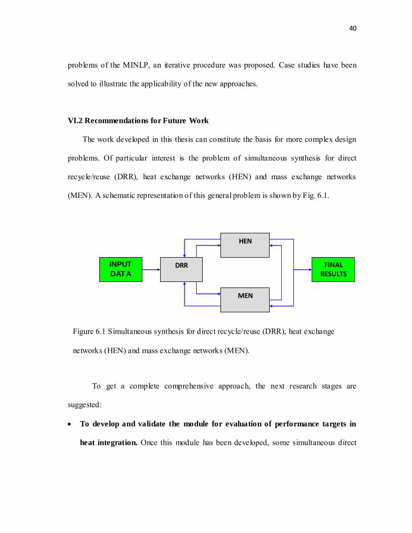
The work developed in this thesis can constitute the basis for more complex design
problems. Of particular interest is the problem of simultaneous synthesis for direct
recycle/reuse (DRR), heat exchange networks (HEN) and mass exchange networks
(MEN). A schematic representation of this general problem is shown by Fig. 6.1.
To get a complete comprehensive approach, the next research stages are
suggested:
To develop and validate the module for evaluation of performance targets in
heat integration. Once this module has been developed, some simultaneous direct
INPUT
DATA DRR
HEN
MEN
FINAL RESULTS
Figure 6.1 Simultaneous synthesis for direct recycle/reuse (DRR), heat exchange
networks (HEN) and mass exchange networks (MEN).

41
recycle and heat integration case studies should be explored. A direct recycle/reuse-
heat exchange modular approach should be validated.
To develop and validate the module for evaluation of performance targets in
mass exchange. This is similar to the case of heat integration. Once this module had
been validated for mass transfer, the mathematical programming platform of LINGO
makes possible to trade off simultaneous performance targets for direct recycle, heat
and mass integration. A new interface for the data section could be convenient to
facilitate this point with which concludes our original objectives in PI.
Exploration for particular applications: Reactive systems could be part of a total
process modeling approach. In addition to physical separation, reactive separation
models could be implemented and the attainable region for reactive systems could be
explored from an even more generic PI perspective. Then, a property-based
framework for process integration could be explored as well.

42
REFERENCES
Almutlaq, A. & El-Halwagi, M. (2007). An algebraic targeting approach to resource conservation via material recycle/reuse. Int. J. Environment and Pollution, 29(1-3), 4-18.
Alva-Argeaz, A., Villianatos, A. & Kokossis, A. (1999) A multicontaminant
transshipment model for mass exchange networks and wastewater minimization problems. Comput. Chem. Eng. 23, 1439.
Alves, J. J. (1999). Analysis and Design of Refinery Hydrogen Distribution Systems. Ph.
D. Thesis, UMIST, Manchester, U.K. Alves J, & Towler G. (2002). Analysis of refinery hydrogen distribution systems. Ind.
Eng. Chem. Res. 41, 5759-5769. Benko, N., Rev, E. & Fonyo, Z. (2000). The use of nonlinear programming to optimal
water allocation. Chemical Eng. Commun. 187, 67. Casanova C. (1981). Excess volumes and excess heat capacities of (water + alkanoic
acid). J. Chem. Thermodynamics, 13, 241-248. Dhole, V. R., Ramchandani, N. & Tanish, R. A. (1996). Make your process water pay
for itself. Chemical Engineering. 103, 100. Dunn, R. F., Wenzel, H. & Overcash, M. R. (2001). Process integration design methods
for water conservation and wastewater reduction in industry: Part I design for single contaminants. J. Clean Prod. Proc. 3, 307.
Dunn, R. F., Wenzel, H. & Overcash M. R. (2001). Process integration design methods
for water conservation and wastewater reduction in industry: Part II design for multiple contaminants. J. Clean Prod. Proc. 3, 319.
Duran, M. A. & Grossman, I. E. (1986) Simultaneous optimization and heat integration of chemical processes. AIChE Journal. 32, 123-138. El-Halwagi M. (2006). Process Integration. San Diego: Academic Press. El-Halwagi, M. M., Gabriel, F. & Harell, D. (2003). Rigorous graphical targeting for
resource conservation via material recycle/reuse networks. Ind. Eng. Chem. Re. 2, 4319-4328.

43
El-Halwagi, M. M. & Manousiouthakis, V. (1990). Simultaneous synthesis of mass-exchange and regeneration networks. AIChE Journal, 36, 1209-1219.
El-Halwagi, M. M. & Manousiouthakis, V. (1989) Synthesis of mass exchange
networks. AIChE Journal, 35, 1233-1244 El-Halwagi, M. M. & Spriggs, H. (1996). An integrated approach to cost and energy
efficient pollution prevention. Fifth World Congress of Chemical Engineering, 344-349.
Gabriel, F. & El-Halwagi, M. M. (2005). Simultaneous synthesis of waste interception
and material reuse networks: problem reformulation for global optimization. Environmental Progress, 24, 171-180.
Hallale, N. (2002). A new graphical targeting method for water minimization. Advances
in Environmental Research, 6, 377-390. Keckler, S. E. & Allen, D. T. (1999). Material reuse modeling: A case study of water
reuse in an industrial park. J. Ind. Ecology. 2, 79-92. Manan, Z. A., Tan Y. L. & Foo, D. C. (2004). Targeting the minimum water flow rate
using water cascade analysis technique. AIChE Journal, 50, 3169-3183. Perry, R. (1998). Perry’s Chemical Engineers’ Handbook. Seventh Edition. New York:
McGraw-Hill. Polley, G. & Polley H. (2000). Design better water networks. Chemical Engineering
Progress, 96, 47-52. Savelski, M. J. & Bagajewicz, M. J. (2000). On the optimality conditions of water
utilization systems in process plants with single contaminants. Chem. Eng. Sci. 56, 5035.
Savelski, M. J. & Bagajewicz, M. J. (2001). Algorithmic procedure to design water
utilization systems featuring a single contaminant in process plants. Chem. Eng. Sci. 56, 1897.
Sorin, M. & Bedard, S. (1999). The global pinch point in water reuse networks. Trans
IChemE. 77, 305-308. Takama, N., Kuriyama, K., Shikoro, K. & Umeda, T. (1980). Optimal water allocation
in a petroleum refinery. Computers and Chemical Engineering, 4, 251-258.

44
Wang, Y. & Smith, R. (1994). Wastewater minimization. Chemical Engineering Science, 49, 981-1006.
Woolley, E. M., Call, T. G., Ford, T. D. & Ballerat-Busserolles, K. (1999). Apparent
molar volumes and heat capacities of aqueous acetic acid and sodium acetate at temperatures from T=278.15 K to 393.15 K at pressure 0.3 MPa. J. Chem. Thermodynamics, 31, 741-762.

45
APPENDIX A
OPTIMIZATION CODING FOR THE VARIABLE SOURCE FORMULATION
MIN = TOTAL_COST;
!*** CONSIDER THE ADITION OF A FINAL FEASIBILITY-PINCH-
PROVE-SCAN!!!
! INTRODUCTION
MODIFIED FILE FOR PROBLEM 3.1
THE GOAL IS TO DEAL WITH SIMULATANEOUS DIRECT RECYCLE,
MASS, HEAT,
OR WHATEVER PROPERTY WHICH CAN BE CHARACTERIZED THROUGH
SOURCES AND
SINKS. THE OBJECTIVE FUNCTION WILL REFLECT SEQUENTIALLY THE
CONSIDE-
RATION OF THESE PROCESS INTEGRATION ATTRIBUTES.
THE BASIC UNIT FOR PROCESS DELIVERING OF PROPERTIES IS THE
"STREAM"
WHICH CAN BE SOURCE,SINK, HOT, COLD, RICH, OR POOR.
DEPENDING ON
WHAT STATE OR INTEGRATION PROPERTY ARE WE DEALING WITH.

46
THE ATTRIBUTES OF THE STREAMS DEFINED THROUGH SET
ATTRIBUTES, AND
SERIES OF SETS ARE DEFINED FOR THE SOLUTION PROCESS.
ATTRIBUTES FOR
THE STREAMS ARE FOR EXAMPLE: INITIAL CONDITIONS, FINAL
CONDIONS, FLOW, CONCENTRATION, ETC.
THE OBJECTIVE FUNCTION WILL BE WEIGHTING ULTIMATELLY IN
TERMS OF
COSTS THE STREAMS COMING FROM THE INPUT DATA. A
SENSITIVITY ANALY-
SIS MUST BE DEVELOPED IF REQUIRED.
DIRECT RECYCLE:;
SETS:
L_CANDIDATE;
L_SINK_COMP;
E_CANDIDATE;
E_SOURCE_COMP;
STREAMS: FEED,STREAM_NO,DRECYCLE, MASS_EXC,
HEAT_EXC,
SOURCE_SINK, RICH_POOR, HOT_COLD,
FLOWRATE,
LOAD, CONCENTRATION;

47
DR_SOURCE_COMP: DR_FLOWRATE_SO, DR_LOAD_SO;
DR_SINK_COMP: DR_FLOWRATE_SI, DR_LOAD_SI;
DR_CANDIDATES: DR_CAND_LOAD, DR_CAND_FLOW,
TOTAL_FLOW_BALANCE,
TOTAL_WASTE_BALANCE,
M_VERTEX, DIST_SO, DIST_FLOW_CAND,
PINCH_FRESHA;
LAMBDA_T_SI(L_CANDIDATE,L_SINK_COMP):
L_T,L_S,SI_FLOW_CAND_INT;
ETA_T_SO(E_CANDIDATE,E_SOURCE_COMP):
E_T,E_S,SO_FLOW_CAND_INT,DR_FLOW_CONT_SO;
MOD(E_CANDIDATE, DR_SINK_COMP): SI_FLOW;
ENDSETS
DATA:
FEED, STREAM_NO ,DRECYCLE, MASS_EXC, HEAT_EXC,
SOURCE_SINK,
1 1 1 0 0 1
1 2 1 0 0 1
1 3 1 0 0 1
1 4 1 0 0 1

48
1 5 1 0 0 1
1 6 1 0 0 0
1 7 1 0 0 0
1 8 1 0 0 0
1 9 1 0 0 0
1 10 1 0 0 0
1 11 1 0 0 0
0 1 1 0 0 1
0 2 1 0 0 1
0 3 1 0 0 1
0 4 1 0 0 1
0 5 1 0 0 1
0 6 1 0 0 0
0 7 1 0 0 0
0 8 1 0 0 0
0 9 1 0 0 0
0 10 1 0 0 0
0 11 1 0 0 0
RICH_POOR, HOT_COLD, FLOWRATE, CONCENTRATION =
0 0 120 0.10
0 0 80 0.14

49
0 0 140 0.18
0 0 80 0.23
0 0 195 0.25
0 0 120 0.0
0 0 80 0.05
0 0 80 0.05
0 0 140 0.140
0 0 80 0.170
0 0 195 0.240
0 0 0 0.00
0 0 0 0.00
0 0 0 0.00
0 0 0 0.00
0 0 0 0.00
0 0 0 0.00
0 0 0 0.00
0 0 0 0.00
0 0 0 0.00
0 0 0 0.00
0 0 0 0.00;
DR_SOURCE_COMP = 1..6; !POINTS IN THE SOURCE COMPOSITE;
DR_SINK_COMP = 1..7; !POINTS IN THE SINK COMPOSITE;

50
DR_CANDIDATES = 1..13; !TOTAL CANDIDATES;
L_CANDIDATE =1..13; !SET FOR BINARY FOR THE
CANDIDATES;
L_SINK_COMP =1..7; !SET FOR BINARY FOR THE SOURCE
COMPOSITE;
E_CANDIDATE =1..13; !SET FOR BINARY FOR THE CANDIDATES
SINK;
E_SOURCE_COMP =1..6; !SET FOR BINARY FOR THE SOURCE
COMPOSITE;
ENDDATA
!This line gives the loads for the set of streams;
!VIRTUAL CALC SECTION
START****************************************;
@FOR(STREAMS(j):LOAD(j)=FLOWRATE(j)*CONCENTRATION(j));

51
@FOR(DR_SOURCE_COMP(J):
DR_FLOWRATE_SO(J)=@IF(J #GT# 1, @SUM(STREAMS(K)|((K#LE#(J-
1))
#AND# (SOURCE_SINK #EQ#
1)):FLOWRATE(K)),0.0););
!FLOWRATE COORDINATE VALUE SOURCE COMPOSITE OK -
1207-07;
@FOR (DR_SOURCE_COMP(J):
DR_LOAD_SO(J)=@IF(J #GT# 1, @SUM(STREAMS(K)| ((K#LE#(J-1))
#AND# (SOURCE_SINK #EQ# 1)):LOAD(K)),0.0););
!LOAD COORDINATE VALUE SOURCE COMPOSITE CURVE ;
@FOR (DR_SINK_COMP(J):
DR_FLOWRATE_SI(J)=@IF(J #GT# 1, @SUM(STREAMS(K)|(K #LE#
(J-1+@SUM(STREAMS(L):SOURCE_SINK(L))/2))
#AND#
(SOURCE_SINK(K) #EQ# 0):FLOWRATE(K)),0.0););
!FLOWRATE COORDINATE VALUE SINK COMPOSITE CURVE;
@FOR (DR_SINK_COMP(J):
DR_LOAD_SI(J) = @IF(J #GT#1, @SUM(STREAMS(K)|(K #LE# (J-
1+@SUM

52
(STREAMS(L):SOURCE_SINK(L))/2)) #AND# (SOURCE_SINK(K)
#EQ# 0):LOAD(K)),!@IF(J #EQ#3,3, ;0.0!);););
!LOAD COORDINATE VALUE SOURCE COMPOSITE CURVE;
! ASSIGNING VALUES TO THE PINCH CANDIDATES;
@FOR (DR_CANDIDATES(J):
DR_CAND_LOAD(J) = @IF(J #LE#
(1+@SUM(STREAMS(L):SOURCE_SINK(L))/2)
,DR_LOAD_SO(J),DR_LOAD_SI(J-
(1+(@SUM(STREAMS(L):SOURCE_SINK(L))/2)
))););
!CASE FOR THE VERTEX IS A POINT FROM THE SINK;
@FOR (DR_CANDIDATES(M)|M #GE# (2+ @SUM(STREAMS(L):
SOURCE_SINK(L))/2):
DR_CAND_FLOW(M) = DR_FLOWRATE_SI(M-
(2+@SUM(STREAMS(Z):SOURCE_SINK(Z))
)/2) );
!CASE FOR THE VERTEX IS A POINT FROM THE SOURCE;
@FOR (DR_CANDIDATES(R)|R #LE# (1 +
@SUM(STREAMS(L):SOURCE_SINK(L))/2):

53
@FOR (DR_SINK_COMP(S):
SI_FLOW(R,S) = @IF((DR_CAND_LOAD(R) #EQ# 0) #OR# (S #EQ#
1),0.0,
@IF((DR_CAND_LOAD(R) #GT# DR_LOAD_SI(S-1))
#AND#
(DR_CAND_LOAD(R) #LT# DR_LOAD_SI(S)),
(DR_CAND_LOAD(R)-DR_LOAD_SI(S-1))/
((DR_LOAD_SI(S)-DR_LOAD_SI(S-
1))/(DR_FLOWRATE_SI(S)
-DR_FLOWRATE_SI(S-1))),
@IF(DR_CAND_LOAD(R) #LT# DR_LOAD_SI(S-
1),0.0,
@IF(DR_CAND_LOAD(R) #GT# DR_LOAD_SI(S),
=DR_FLOWRATE_SI(S)-DR_FLOWRATE_SI(S-
1),0!*****;););
);););
DR_CAND_FLOW(R) = @SUM(MOD(R,k):SI_FLOW(R,k););
);
!MODIFIERS: I.P.H.E.S.;

54
@FOR (DR_CANDIDATES(i)|i #GE# (2+
@SUM(STREAMS(L):SOURCE_SINK(L))/2)
:
@FOR (DR_SOURCE_COMP(j):
DR_FLOW_CONT_SO(i,j)= @IF((DR_CAND_LOAD(i) #EQ# 0)
#OR#
(j #EQ# 1),0.0,
@IF(DR_CAND_LOAD(i) #EQ#
DR_LOAD_SO(j-1),0.0,
@IF(DR_CAND_LOAD(i) #EQ#
DR_LOAD_SO(j),
DR_FLOWRATE_SO(j),
@IF( (DR_CAND_LOAD(i) #LT# DR_LOAD_SO(j)) #AND#
(DR_CAND_LOAD(i) #GT# DR_LOAD_SO(j-1)),
(DR_CAND_LOAD(i)-DR_LOAD_SO(j-1))/((DR_LOAD_SO(j)-
DR_LOAD_SO(j-1))
/(DR_FLOWRATE_SO(j)-DR_FLOWRATE_SO(j-1))),
!***Few; @IF(DR_CAND_LOAD(i) #LT# DR_LOAD_SO(j-
1),0.0,
@IF(DR_CAND_LOAD(i) #GT#
DR_LOAD_SO(j),DR_FLOWRATE_SO(j),0!******;
);););););));
DIST_SO(i)= @SUM(ETA_T_SO(i,k):DR_FLOW_CONT_SO(i,k));

55
DIST_FLOW_CAND(i)= DR_CAND_FLOW(i)-DIST_SO(i);
);
!6666 stands for silly error in the calculation;
!BINARY VARIABLES FOR DIRECT RECYCLE PLUS...;
!LOOPING FOR LOAD CALCULATION EVERY SPECIFIC PINCH
CANDIDATES;
!FLOW REQ. FOR EVERY INTERVAL IN ALL THE CANDIDATES -
SOURCES-?;
@FOR (DR_CANDIDATES(i):
@FOR (DR_SOURCE_COMP(j):
E_S(i,j)= @IF(j #LE# (@SUM(STREAMS(L):SOURCE_SINK))/2,
@IF(DR_LOAD_SO(j+1) #GE#
DR_CAND_LOAD(i),0,1),0!*******;);
E_T(i,j)= @IF(j #LE# (@SUM(STREAMS(L):SOURCE_SINK))/2,
@IF(DR_LOAD_SO(j) #GE#
DR_CAND_LOAD(i),0,1),0!******;);
SO_FLOW_CAND_INT(i,j) = @IF(j #LE# (@SUM(STREAMS(L):
SOURCE_SINK))/2,E_T(i,j)*(DR_CAND_FLOW(i)-
DR_FLOWRATE_SO(j)
-DIST_FLOW_CAND(i))
-E_S(i,j)*(DR_CAND_FLOW(i)-DR_FLOWRATE_SO(j+1)

56
-DIST_FLOW_CAND(i)),0.0);
);
);
!FLOWS REQ. FOR EVERY INTERVAL IN ALL THE CANDIDATES -
SINKS-?;
@FOR (DR_CANDIDATES(i):
@FOR (DR_SINK_COMP(j):
L_S(i,j)= @IF(j #LE# (@SUM(STREAMS(L):DRECYCLE(L))/2-
@SUM(STREAMS(L):SOURCE_SINK(L))/2),
@IF(DR_LOAD_SI(j) #GE# DR_CAND_LOAD(i),0,1),0!*****;);
L_T(i,j)= @IF(j #LE# (@SUM(STREAMS(L):DRECYCLE(L))/2-
@SUM(STREAMS(L):SOURCE_SINK(L))/2),
@IF(DR_LOAD_SI(j+1) #GE#
DR_CAND_LOAD(i),0,1),0!******;);
SI_FLOW_CAND_INT(i,j) = @IF(j #LE# (@SUM(STREAMS(L):
DRECYCLE(L))/2-@SUM(STREAMS(L):SOURCE_SINK(L))/2),
L_S(i,j)*(DR_CAND_FLOW(i)-DR_FLOWRATE_SI(j))-L_T(i,j)*
(DR_CAND_FLOW(i)-DR_FLOWRATE_SI(j+1)),0.0);
);
);

57
!BALANCE OF FLOWS: (EQ. 22) TOTAL FLOW FOR THE SET OF
CANDIDATES note %%% ;!BELOW THE PINCH... FRESH STREAM;
@FOR (DR_CANDIDATES(i):
TOTAL_FLOW_BALANCE(i) = @SUM (LAMBDA_T_SI(i,k):
SI_FLOW_CAND_INT(i,k)) -
@SUM (ETA_T_SO(i,k):SO_FLOW_CAND_INT(i,k));
);
@FOR (DR_CANDIDATES(i):
TOTAL_WASTE_BALANCE(i) = @SUM(DR_SINK_COMP(J)|J #LE#
(@SUM(STREAMS(L):DRECYCLE(L))/2 -
@SUM(STREAMS(L):SOURCE_SINK(L))/2):
(DR_FLOWRATE_SI(J+1)-DR_FLOWRATE_SI(J)))-@SUM
(DR_SOURCE_COMP(J)|J#LE#5 :(DR_FLOWRATE_SO(J+1)
-DR_FLOWRATE_SO(J)))-TOTAL_FLOW_BALANCE(i)
);
@FOR (DR_CANDIDATES(J):
PINCH_FRESHA(J) = @IF(TOTAL_WASTE_BALANCE #EQ#
@MIN(DR_CANDIDATES(R):TOTAL_WASTE_BALANCE(R)),
@ABS(TOTAL_FLOW_BALANCE(J)),0.0);
);

58
PINCH_FRESH = @MAX(DR_CANDIDATES(J):PINCH_FRESHA);
!***THE ONLY ONE WITH A VALUE DIFFERENT THAN 0.0;
!VIRTUAL CALC SECTION
END******************************************;
PINCH_WASTE =-1*@MIN(DR_CANDIDATES:TOTAL_WASTE_BALANCE);
TOTAL_COST = PINCH_FRESH + PINCH_WASTE;
!RESTRICTIONS... solver fails!!!;
!FLOWRATE(1) >0; !CONCENTRATION(1)>0.0;
!FLOWRATE(2) >0; !CONCENTRATION(2)>0.0;
!FLOWRATE(3) >0; !CONCENTRATION(3)>0.0;
!FLOWRATE(4) >0; !CONCENTRATION(4)>0.0;
!FLOWRATE(5) >0; !CONCENTRATION(5)>0.0;
!FLOWRATE(6) >=0; !CONCENTRATION(6)>=0.0;
!FLOWRATE(7) >0; !CONCENTRATION(7)>0.0;
!FLOWRATE(8) >0; !CONCENTRATION(8)>0.0;
!FLOWRATE(9) >0; !CONCENTRATION(9)>0.0;
!FLOWRATE(10)>0; !CONCENTRATION(10)>0.0;
!FLOWRATE(11)>0; !CONCENTRATION(11)>0.0;
!FLOWRATE(12)=0;
!FLOWRATE(13)=0;

59
!FLOWRATE(14)=0;
!FLOWRATE(15)=0;
!FLOWRATE(16)=0;
!FLOWRATE(17)=0;
!FLOWRATE(18)=0;
!FLOWRATE(19)=0;
!FLOWRATE(20)=0;
!FLOWRATE(21)=0;
!FLOWRATE(22)=0;
!FLOWRATE(1) =120; !CONCENTRATION(1)<0.1;
!FLOWRATE(2) =80; !CONCENTRATION(2)<0.14;
!FLOWRATE(3) =140; !CONCENTRATION(3)<0.18;
!FLOWRATE(4) =80; !CONCENTRATION(4)<0.23;
!FLOWRATE(5) =195; !CONCENTRATION(5)<0.25;
!FLOWRATE(6) =120; !CONCENTRATION(6)<0.0;
!FLOWRATE(7) =80; !CONCENTRATION(7)<0.05;
!FLOWRATE(8) =80; !CONCENTRATION(8)<0.05;
!FLOWRATE(9) =140; !CONCENTRATION(9)<0.140;
!FLOWRATE(10)=80; !CONCENTRATION(10)<0.170;
!FLOWRATE(11)>193;
!FLOWRATE(11)<195; !CONCENTRATION(11)<0.240;

60
!PINCH_WASTE>0;
!PINCH_FRESH>0;
END

61
VITA
Jose Guadalupe Zavala Oseguera
B. Eng. University of Guanajuato, Mexico (1999);
M. Eng. University of Guanajuato, Mexico (2004);
M. Sci. University of Texas A&M, U. S. (2008)
Address: Chamizal No. 10 A Colonia Centro, Moroleón, Gto. México. C. P. 38800. [email protected]


![Reduce Reuse Recycle[1]](https://img.dokumen.tips/doc/110x75/5528136655034684588b464f/reduce-reuse-recycle1.jpg)