Embed Size (px)
Citation preview
Design of driven piles and drilled shaft
foundations
NCHRP 368
Chapter 8
pages 57 to 64

The bearing resistance and settlement
behavior of driven piles and drilled shafts can
be calculated in two manners:
1. Indirect methods that use conventional soil
mechanics methods.
1. su, f’, E’, Eu, and cv determined from correlation with qt,
fs, u2, vs and pore pressure dissipation tests.
2. cc and cr determined from lab consolidation tests.
2. Direct methods that incorporate a combination of the
measured cone tip resistance, sleeve resistance or
pore pressure data in the formulae.

Direct methods for nominal axial resistance
analysis of driven piles and drilled shafts
• LCPC method (1982) summarized in NCHRP 368, also
in FHWA-SA-91-043, The Cone Penetrometer Test
• Norwegian Geotechnical Institute method (1996, 2001)
in NCHRP 368
• Politecnico di Torino method (1995) in NCHRP 368
• Unicone method (1997, 2006) in NCHRP 368
• Takesue method (1998) in NCHRP 368
RR = (f) (Rn) = (fstat) (Rnstat) = (f) (Qn)
f or fstat <= 0.7 is recommended in
Caltrans amendments to the LRFD BDS
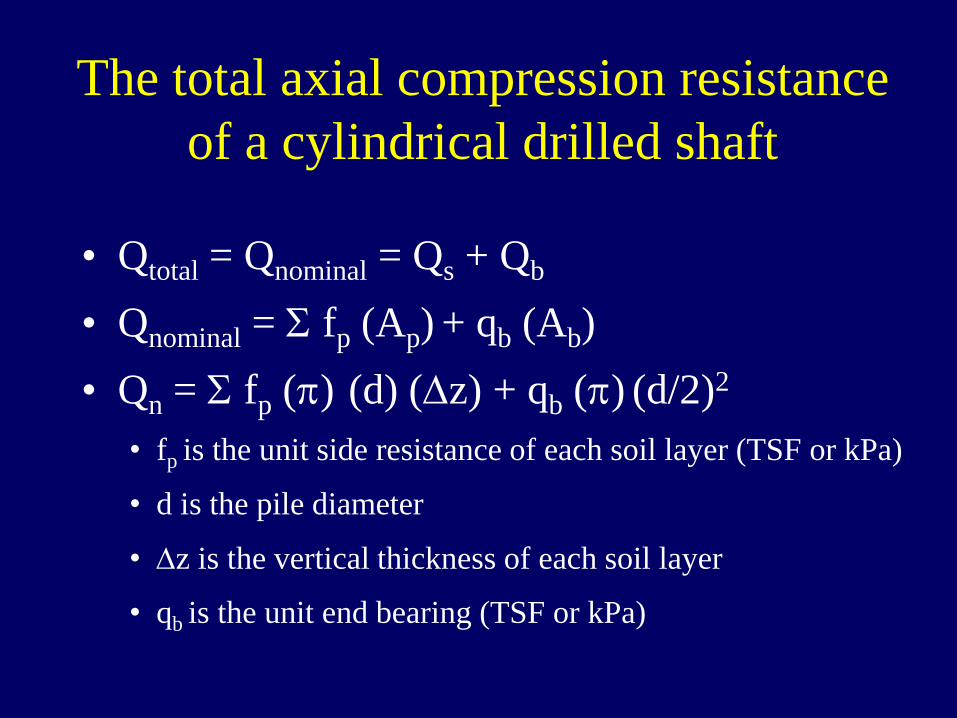
The total axial compression resistance
of a cylindrical drilled shaft
• Qtotal = Qnominal = Qs + Qb
• Qnominal = S fp (Ap) + qb (Ab)
• Qn = S fp (p) (d) (Dz) + qb (p) (d/2)2
• fp is the unit side resistance of each soil layer (TSF or kPa)
• d is the pile diameter
• Dz is the vertical thickness of each soil layer
• qb is the unit end bearing (TSF or kPa)
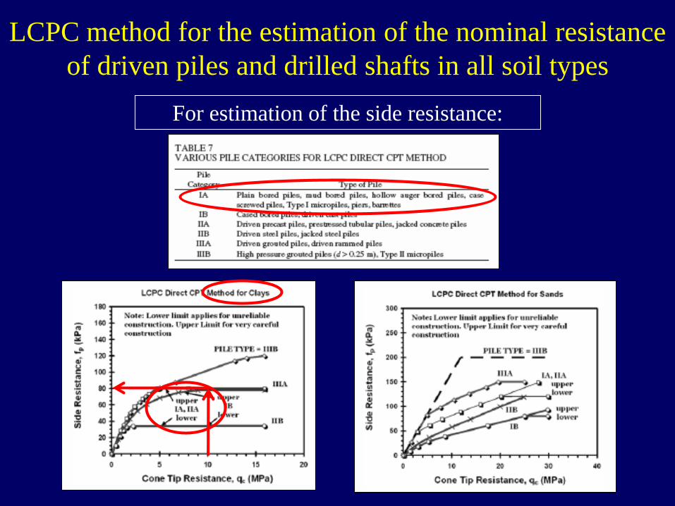
LCPC method for the estimation of the nominal resistance
of driven piles and drilled shafts in all soil types
For estimation of the side resistance:
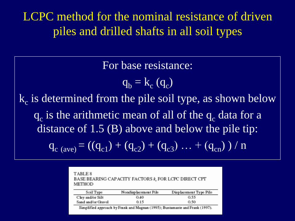
LCPC method for the nominal resistance of driven
piles and drilled shafts in all soil types
For base resistance:
qb = kc (qc)
kc is determined from the pile soil type, as shown below
qc is the arithmetic mean of all of the qc data for a
distance of 1.5 (B) above and below the pile tip:
qc (ave) = ((qc1) + (qc2) + (qc3) … + (qcn) ) / n
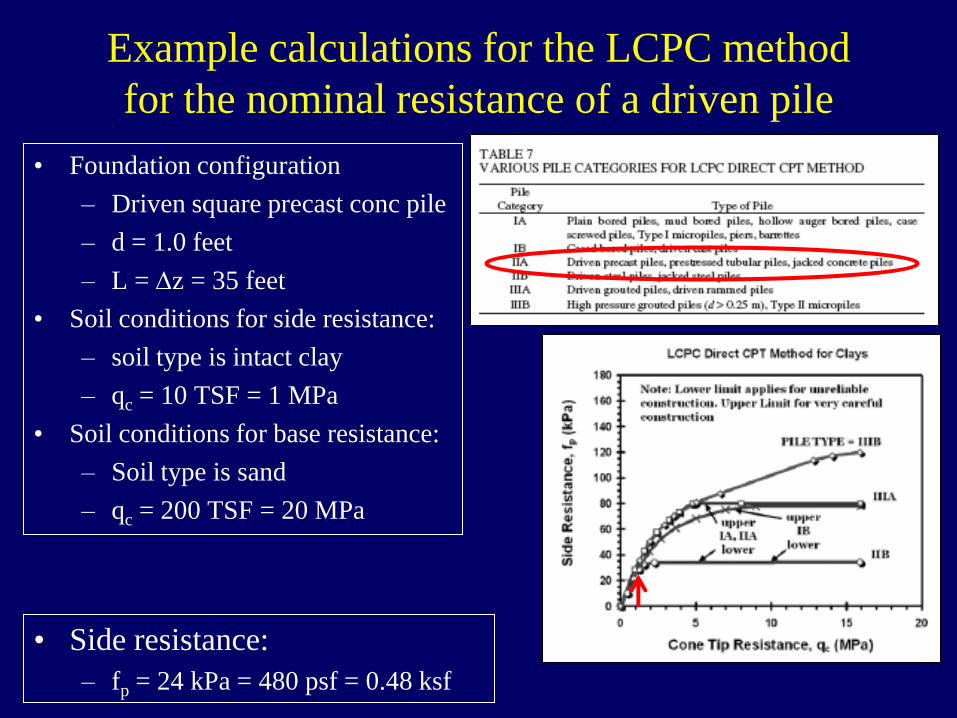
Example calculations for the LCPC method
for the nominal resistance of a driven pile
• Foundation configuration
– Driven square precast conc pile
– d = 1.0 feet
– L = Dz = 35 feet
• Soil conditions for side resistance:
– soil type is intact clay
– qc = 10 TSF = 1 MPa
• Soil conditions for base resistance:
– Soil type is sand
– qc = 200 TSF = 20 MPa
• Side resistance:
– fp = 24 kPa = 480 psf = 0.48 ksf

Example calculations using the LCPC method
for the nominal resistance of a driven pile
• Foundation configuration
– Driven square precast conc pile
– d = 1.0 feet
– L = Dz = 35 feet
• Soil conditions for side resistance:
– soil type is intact clay
– qc = 10 TSF
• Soil conditions for base resistance:
– Soil type is sand
– qc = 200 TSF
• Base resistance:
– qb = kc (qc)
– qb = 0.50 (400 ksf) = 200 ksf
Qnominal = S fp (Ap) + qb (Ab)
Qnominal = 0.48 ksf (35) (4) + 200 (1)
Qnominal = 67 + 200 = 267 kips

Norwegian Geotechnical Institute method for the
nominal resistance of driven piles in cohesive soil
For side resistance:
fp = (qt –sv0) / (10.5 + 13.3 (log Q))
Q = normalized cone tip resistance
Q = (qt – sv0) / sv0’
For base resistance:
qb = (qt – sv0) / k2
k2 = Nkt / 9
Nkt = 15 for soft to firm intact clays
All terms are assumed to be in units of MPa.

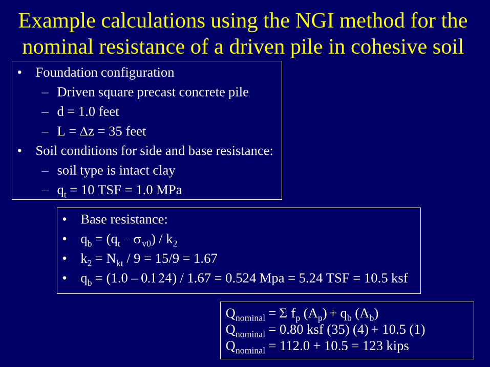
Example calculations for the NGI method for the
nominal resistance of a driven pile in cohesive soil
• Foundation configuration
– Driven square precast concrete pile
– d = 1.0 feet
– L = Dz = 35 feet
• Soil conditions for side and base resistance:
– soil type is intact clay
– qt = 10 TSF = 1.0 Mpa
• Side resistance:
• fp = (qt –sv0) / (10.5 + 13.3 (log Q))
• Q = (qt – sv0) / sv0’
• sv0 = sv0’ = (5 + 35/2) (0.110/2) = 1.24 TSF = 0.124 MPa
• Q = (1.0 – 0.124)/0.124 = 7.06
• fp = (1.0 – 0.124) / (10.5 + 13.3 (log 7.06))
• fp = 0.876 / 21.79 = 0.0402 Mpa = 40.2 kPa = 0.80 ksf
Example calculations using the NGI method for the
nominal resistance of a driven pile in cohesive soil• Foundation configuration
– Driven square precast concrete pile
– d = 1.0 feet
– L = Dz = 35 feet
• Soil conditions for side and base resistance:
– soil type is intact clay
– qt = 10 TSF = 1.0 MPa
• Base resistance:
• qb = (qt – sv0) / k2
• k2 = Nkt / 9 = 15/9 = 1.67
• qb = (1.0 – 0.124) / 1.67 = 0.524 Mpa = 5.24 TSF = 10.5 ksf
Qnominal = S fp (Ap) + qb (Ab)
Qnominal = 0.80 ksf (35) (4) + 10.5 (1)
Qnominal = 112.0 + 10.5 = 123 kips
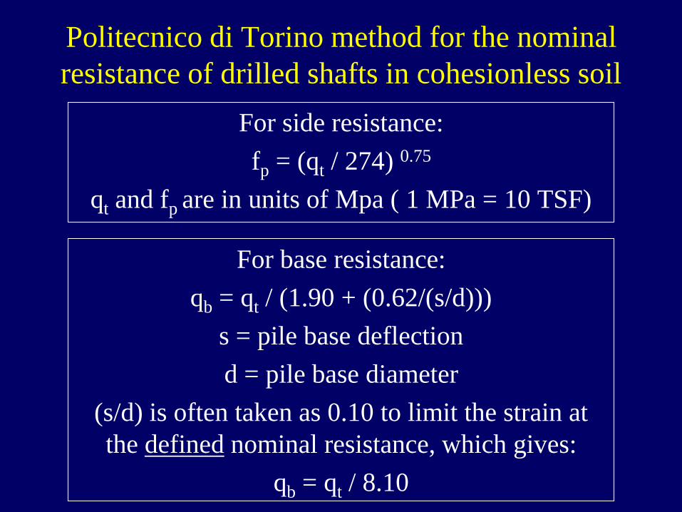
Politecnico di Torino method for the nominal
resistance of drilled shafts in cohesionless soil
For side resistance:
fp = (qt / 274) 0.75
qt and fp are in units of Mpa ( 1 MPa = 10 TSF)
For base resistance:
qb = qt / (1.90 + (0.62/(s/d)))
s = pile base deflection
d = pile base diameter
(s/d) is often taken as 0.10 to limit the strain at
the defined nominal resistance, which gives:
qb = qt / 8.10

Example calculations using the Politecnico di Torino method
for the nominal resistance of a drilled shaft in cohesionless soil
• Foundation configuration
– Drilled shaft without casing support
– d = 2.0 feet = 0.61 meter
– L = Dz = 35 feet = 10.67 meters
• Soil conditions for side and base resistance:
– soil type: sand
– qt = 70 TSF = 7.0 MPa
• fp = (qt / 274) 0.75
• fp = (7.0 / 274) 0.75 = 0.0639 MPa = 0.639 TSF = 1.3 ksf
• qb = qt / 8.10
• qb = 7.0 / 8.10 = 0.864 MPa = 8.64 TSF = 17.3 ksf
Qnominal = S fp (Ap) + qb (Ab)
Qnominal = 1.3 ksf (35) (p) (2.0) + 17.3 (p) (1)2
Qnominal = 285.9 + 54.3 = 340 kips

Unicone method (Eslami and Fellenius) for
the nominal resistance of driven piles or
drilled shafts in all soil types
For side resistance:
fp = Cse (qE)
Cse is from Table 9 based on the soil classes from the Figure below
qE = (qt – u2) in MPa

Unicone method (Eslami and Fellenius) for
the nominal resistance of driven piles or
drilled shafts in all soil types
For base resistance:
qb = Cte (qE)
Cte is generally taken as 1.0
qE = (qt – u2) in MPa
If the effective cone resistance profile (qE) indicates
significant variation, the authors recommend a geometric,
not arithmetic mean be calculated:
qE (ave) = ((qE1) (qE2) (qE3) … (qEn) )1/n
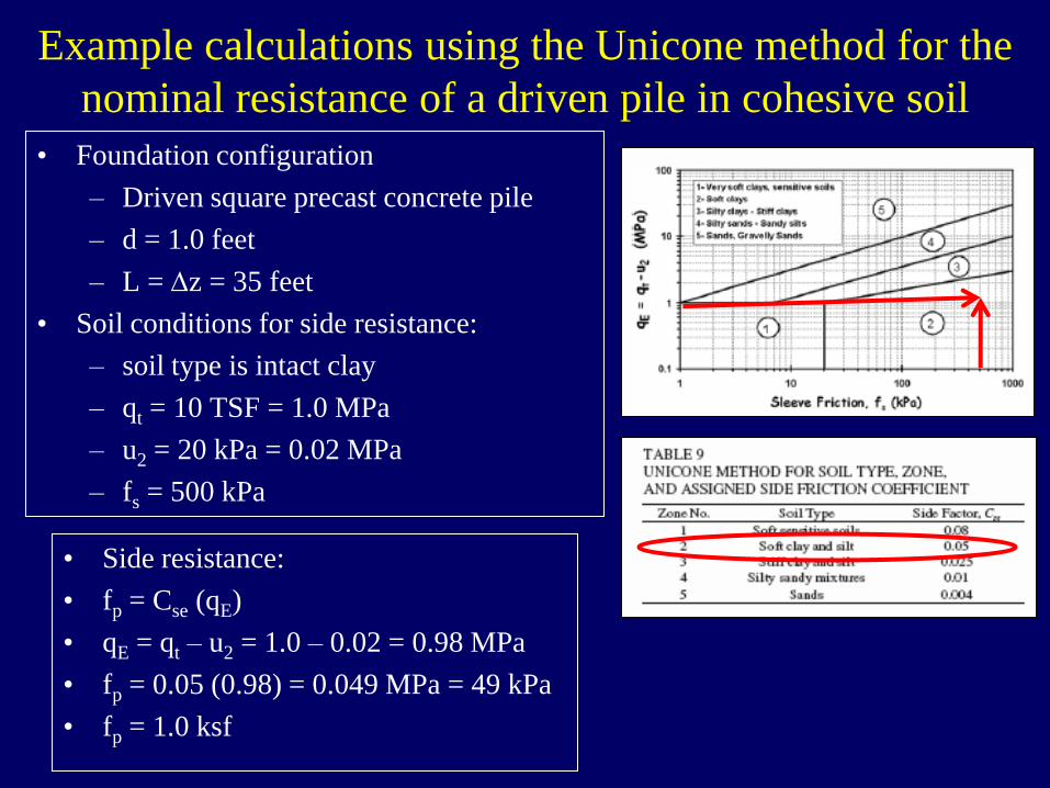
Example calculations using the Unicone method for the
nominal resistance of a driven pile in cohesive soil
• Foundation configuration
– Driven square precast concrete pile
– d = 1.0 feet
– L = Dz = 35 feet
• Soil conditions for side resistance:
– soil type is intact clay
– qt = 10 TSF = 1.0 MPa
– u2 = 20 kPa = 0.02 MPa
– fs = 500 kPa
• Side resistance:
• fp = Cse (qE)
• qE = qt – u2 = 1.0 – 0.02 = 0.98 MPa
• fp = 0.05 (0.98) = 0.049 MPa = 49 kPa
• fp = 1.0 ksf

Example calculations for the Unicone method for the
nominal resistance of a driven pile in cohesive soil
• Foundation configuration
– Driven square precast concrete pile
– d = 1.0 feet
– L = Dz = 35 feet
• Soil conditions for base resistance:
– soil type is intact clay
– qt = 10 TSF = 1.0 MPa
– u2 = 20 kPa = 0.02 MPa
• Base resistance:
• qb = Cte (qE)
• qE = qt – u2 = 1.0 – 0.02 = 0.98 MPa
• qb = 1.0 (0.98) = 0.98 MPa
• qb = 9.8 TSF = 19.8 ksfQnominal = S fp (Ap) + qb (Ab)
Qnominal = 1.0 ksf (35) (4) + 19.8 (1)
Qnominal = 140 + 19.8 = 160 kips
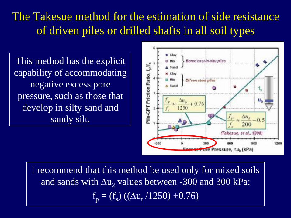
The Takesue method for the estimation of side resistance
of driven piles or drilled shafts in all soil types
This method has the explicit
capability of accommodating
negative excess pore
pressure, such as those that
develop in silty sand and
sandy silt.
I recommend that this method be used only for mixed soils
and sands with Du2 values between -300 and 300 kPa:
fp = (fs) ((Dut /1250) +0.76)

Example calculations using the Takesue method for the
nominal resistance of a drilled shaft in cohesionless soil
• Foundation configuration
– Drilled shaft without casing support
– d = 2.0 feet = 0.61 meter
– L = Dz = 35 feet = 10.67 meters
• Soil conditions for side and base resistance:
– soil type: sand
– qt = 70 TSF = 7.0 MPa
– fs = 100 kPa
– Dut = 8 kPa
• fp = (fs) ((Dut /1250) +0.76)
• fp = (100) ((8/1250) + 0.76) = 76.6 kPa = 1.5 ksf
• qb = 7.0 / 8.10 = 0.864 MPa = 8.64 TSF = 17.3 ksf from Politecnico method
Qnominal = S fp (Ap) + qb (Ab)
Qnominal = 1.5 ksf (35) (p) (2.0) + 17.3 (p) (1)2
Qnominal = 329.9 + 54.3 = 384 kips

Indirect methods for estimating the settlement of
a single driven pile or drilled shaft
1. Approximate nonlinear methods for the immediate
(drained) component of settlement for driven piles or
drilled shafts embedded in cohesionless soils
2. Approximate nonlinear method for the immediate
(undrained) component of settlement for driven piles or
drilled shafts embedded in cohesive soils
3. Approximate nonlinear method for the recompression
portion of consolidation (drained) for driven piles or
drilled shafts embedded in cohesive soils
4. Conventional consolidation analysis for the virgin
compression component of settlement. The pattern of
stress distribution into the soil must be developed using a
procedure such as the equivalent footing concept.

Approximate nonlinear method for the immediate settlement of
one driven pile or one drilled shaft embedded in cohesionless soil
wt = displacement at the top of the driven pile or drilled shaft
Qt = Service Limit State Load on the pile
Ir = influence factor
d = pile diameter
E’ = Young’s modulus for drained conditions
E’ = E0 (1 – (Qt /Qn)0.3) where E0 is the drained small strain
Young’s modulus determined from vs and n’
wt = ((Qt) (Ir)) / ((d) (E’))
Ir = 1/(((1/(1 – (n’)2)) + (p/(1 + n’)) ((L/d) / (ln (5(L/d) (1 – n’)))))
n’ = poisson’s ratio for drained conditions = 0.20

Approximate nonlinear method for the immediate settlement of
one driven pile or one drilled shaft embedded in cohesive soil
wt = displacement at the top of the driven pile or drilled shaft
Qt = Service Limit State Load
Ir = influence factor
d = pile diameter
Eu = Young’s modulus for undrained conditions
Eu = E0 (1 – (Qt /Qn)0.3) where E0 is the undrained small strain
Young’s modulus determined from vs and nu
wt = ((Qt) (Ir)) / ((d) (Eu))
Ir = 1/(((1/(1 – (nu)2)) + (p/(1 + nu)) ((L/d) / (ln (5(L/d) (1 – nu)))))
nu = poisson’s ratio for undrained conditions = 0.50
The calculation accounts for the portion of the applied pile
load (Q) which results in a soil stress that is less than sp’.

Approximate nonlinear method for the recompression portion of
consolidation for one driven pile or one drilled shaft embedded
in cohesive soil
This calculation accounts for the portion of the applied
pile load (Q) which results in a soil stress that exceeds sp’.
This stress causes consolidation.
wt = ((Qt) (Ir)) / ((d) (E’))
wt = displacement at the top of the driven pile or drilled shaft
Qt = Service Limit State Load
Ir = influence factor
d = pile diameter
E’ = Young’s modulus for drained conditions
E’ = E0 (1 – (Qt /Qn)0.3) where E0 is the drained small strain
Young’s modulus determined from vs and n’
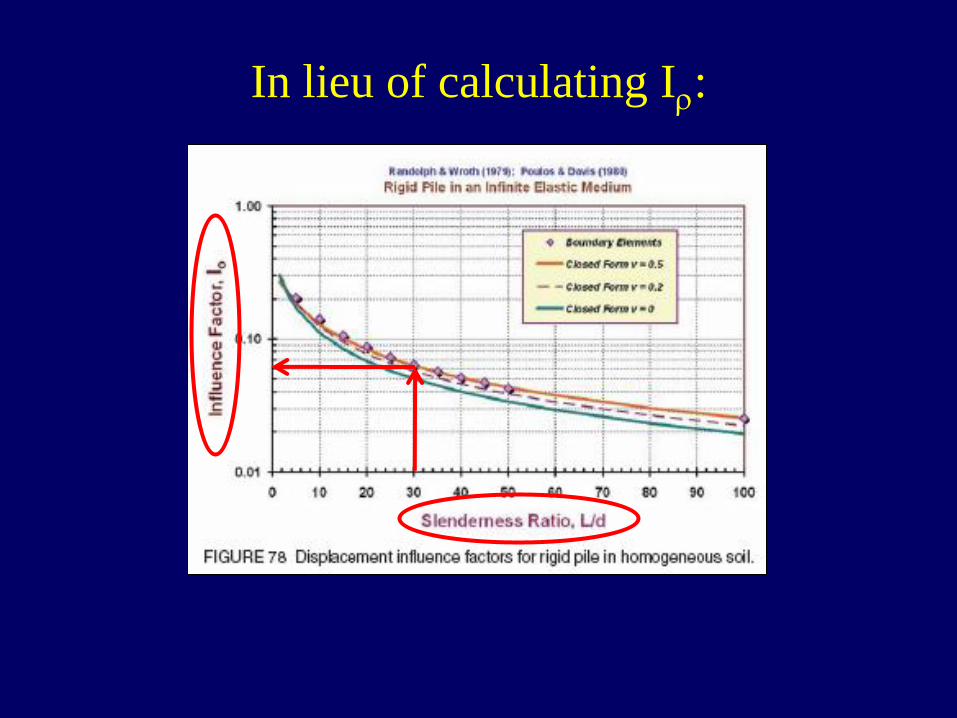
In lieu of calculating Ir:
Summary and recommendations
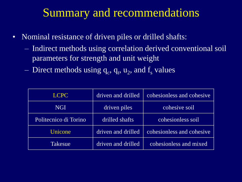
• Nominal resistance of driven piles or drilled shafts:
– Indirect methods using correlation derived conventional soil
parameters for strength and unit weight
– Direct methods using qc, qt, u2, and fs values
LCPC driven and drilled cohesionless and cohesive
NGI driven piles cohesive soil
Politecnico di Torino drilled shafts cohesionless soil
Unicone driven and drilled cohesionless and cohesive
Takesue driven and drilled cohesionless and mixed
Summary and recommendations
• Settlement calculations for deep foundations:
– Indirect method based on approximate nonlinear theory using
correlation derived E’ and E0
– Conventional consolidation analysis based on lab test results.
– There are no direct methods available for settlement analysis.

Exercise 4
Determining the nominal bearing
resistance of a driven pile