Embed Size (px)
Citation preview

Design of bi-orthogonal rational
Discrete Wavelet Transform and the
associated applications
by
Nguyen, Nguyen Si Tran
B. Eng. (Information Technology and Telecommunication, with first class Honours),The University of Adelaide, Australia, 2007
Thesis submitted for the degree of
Doctor of Philosophy
in
Electrical and Electronic Engineering,
Faculty of Engineering, Computer and Mathematical Sciences
The University of Adelaide, Australia
2014

Supervisors:
Dr Brian W.-H. Ng, School of Electrical & Electronic Engineering
Prof Langford B White, School of Electrical & Electronic Engineering
© 2014
Nguyen, Nguyen Si Tran
All Rights Reserved
Contents
Contents iii
Abstract vii
Statement of Originality ix
Acknowledgments xi
Thesis Conventions xiii
Publications xv
List of Figures xvii
List of Tables xxi
Chapter 1. Introduction 1
1.1 Introduction . . . . . . . . . . . . . . . . . . . . . . . . . . . . . . . . . . . 2
1.2 Open questions to address . . . . . . . . . . . . . . . . . . . . . . . . . . . 4
1.3 Overview of the thesis . . . . . . . . . . . . . . . . . . . . . . . . . . . . . 4
1.4 Background on Time-frequency analysis . . . . . . . . . . . . . . . . . . . 5
1.4.1 Short Time Fourier analysis . . . . . . . . . . . . . . . . . . . . . . 6
1.4.2 Wavelet transforms . . . . . . . . . . . . . . . . . . . . . . . . . . . 8
1.4.3 Wavelet transforms based on uniform M-channel FBs . . . . . . . 16
1.4.4 Rational rate filter banks (RFB) and rational discrete wavelets . . 18
1.5 Contributions and Publications . . . . . . . . . . . . . . . . . . . . . . . . 22
1.6 Chapter summary . . . . . . . . . . . . . . . . . . . . . . . . . . . . . . . . 23
Chapter 2. Iterated RFB - Design challenges and literature works 25
2.1 Iterated rational filter bank designs - Design challenges . . . . . . . . . . 26
Page iii
Contents
2.1.1 Aliasing in NUFBs structure – summary of necessary conditions
for PR non-uniform FB . . . . . . . . . . . . . . . . . . . . . . . . . 26
2.1.2 The issue of shift variance in iterated RFB . . . . . . . . . . . . . . 31
2.2 Existing Design approaches in the literature . . . . . . . . . . . . . . . . . 34
2.2.1 Critically sampled RFBs and RADWTs . . . . . . . . . . . . . . . 35
2.2.2 Overcomplete RFB – redundant RADWTs . . . . . . . . . . . . . . 39
2.3 Chapter summary . . . . . . . . . . . . . . . . . . . . . . . . . . . . . . . . 43
Chapter 3. Bi-orthogonal RFB for Fine Frequency Decomposition: the ( q−1q , 1
q )
case 45
3.1 Introduction and motivation . . . . . . . . . . . . . . . . . . . . . . . . . . 46
3.2 Design of two-channel rational filter banks . . . . . . . . . . . . . . . . . 47
3.2.1 Perfect reconstruction filter bank . . . . . . . . . . . . . . . . . . . 50
3.2.2 Vanishing moments and regularity orders . . . . . . . . . . . . . . 51
3.2.3 Least square optimisation . . . . . . . . . . . . . . . . . . . . . . . 54
3.3 Solving the design problem . . . . . . . . . . . . . . . . . . . . . . . . . . 55
3.3.1 Local optimisation of the non-linear problem . . . . . . . . . . . . 55
3.3.2 Linearisation of the non-linear constraints . . . . . . . . . . . . . 59
3.4 Filter design results . . . . . . . . . . . . . . . . . . . . . . . . . . . . . . . 61
3.5 Shift error and computational complexity . . . . . . . . . . . . . . . . . . 65
3.6 Chapter summary . . . . . . . . . . . . . . . . . . . . . . . . . . . . . . . . 67
Chapter 4. Bi-orthgonal RFB structure of (pq ,
q−pq ) - flexible Q factor transforms 69
4.1 Introduction and motivation . . . . . . . . . . . . . . . . . . . . . . . . . . 70
4.2 Regular perfect reconstruction rational FBs . . . . . . . . . . . . . . . . . 71
4.2.1 Perfect reconstruction (PR) FBs . . . . . . . . . . . . . . . . . . . . 71
4.2.2 Regularity . . . . . . . . . . . . . . . . . . . . . . . . . . . . . . . . 73
4.3 Design algorithm . . . . . . . . . . . . . . . . . . . . . . . . . . . . . . . . 77
4.3.1 Iterative algorithm . . . . . . . . . . . . . . . . . . . . . . . . . . . 79
4.4 Design Results . . . . . . . . . . . . . . . . . . . . . . . . . . . . . . . . . . 80
4.5 Convergence of the algorithm and remarks . . . . . . . . . . . . . . . . . 87
4.6 Chapter summary . . . . . . . . . . . . . . . . . . . . . . . . . . . . . . . . 90
Page iv

Contents
Chapter 5. Biorthogonal RADWT: Applications and discussions 93
5.1 Introduction . . . . . . . . . . . . . . . . . . . . . . . . . . . . . . . . . . . 94
5.2 Speech signal processing . . . . . . . . . . . . . . . . . . . . . . . . . . . . 95
5.2.1 Comparing sparsity measures of TIMIT speech signals . . . . . . 95
5.2.2 Denoising of TIMIT speech signals based on RADWTs . . . . . . 97
5.2.3 Speech signal decomposition . . . . . . . . . . . . . . . . . . . . . 102
5.3 Chirp signal separation from narrow band interference . . . . . . . . . . 105
5.3.1 Chirp signal separation from prolonged sinusoidal interference . 105
5.3.2 Chirp signal separation from short burst interference . . . . . . . 108
5.4 Concluding remarks and summary . . . . . . . . . . . . . . . . . . . . . . 111
Chapter 6. Thesis conclusion and future work 115
6.1 Introduction . . . . . . . . . . . . . . . . . . . . . . . . . . . . . . . . . . . 116
6.2 Thesis summary conclusion . . . . . . . . . . . . . . . . . . . . . . . . . . 116
6.3 Potential future work . . . . . . . . . . . . . . . . . . . . . . . . . . . . . . 117
6.4 Original contributions . . . . . . . . . . . . . . . . . . . . . . . . . . . . . 118
6.5 In closing . . . . . . . . . . . . . . . . . . . . . . . . . . . . . . . . . . . . . 119
Appendix A. 121
A.1 Detailed derivation of the regularity condition relationship . . . . . . . . 122
A.2 Relationship between filter’s polyphase component and its passband
flatness . . . . . . . . . . . . . . . . . . . . . . . . . . . . . . . . . . . . . . 124
Appendix B. Filter design results 127
B.1 RFB designed by linearised method with parameters satisfying ( q−1q , 1
q ) 128
B.1.1 Rational filter bank of (23 , 1
3) . . . . . . . . . . . . . . . . . . . . . . 128
B.1.2 Rational filter bank of (34 , 1
4) . . . . . . . . . . . . . . . . . . . . . . 128
B.1.3 Rational filter bank of (67 , 1
7) . . . . . . . . . . . . . . . . . . . . . . 128
B.1.4 Rational filter bank of ( 910 , 1
10) . . . . . . . . . . . . . . . . . . . . . 130
Bibliography 133
Glossary 141
Page v

Page vi

Abstract
Time-frequency analysis has long been a very useful tool in the field of signal process-
ing, especially in dealing with non-stationary signals. Wavelet transform is amongst
many time-frequency analysis techniques whose attributes have been well exploited in
many classic applications such as de-noising and compression. In recent years, repre-
sentation sparsity, a measure of the representation’s ability to condense signals’ energy
into few coefficients, has raised much interest from researchers in many fields such as
signal processing, information theory and applied mathematics due to its wide range
of use. Thus, many classes of time-frequency representations have recently been de-
veloped from the conventional ones in maximising the representation sparsity recently.
Rational discrete wavelet transform (RADWT), an extended class of the conventional
wavelet family, is among those representations. This thesis discusses the design of
bi-orthogonal rational discrete wavelet transform which is constructed from finite im-
pulse response (FIR) two-channel rational rate filter banks and the associated potential
applications. Techniques for designing the bi-orthogonal rational filter bank are pro-
posed, their advantages and disadvantages are discussed and compared with the ex-
isting designs in literature. Experimental examples are provided to illustrate the use of
the novel bi-orthogonal RADWT in application such as signal separation. The exper-
iments show sparser signal representations with RADWTs over conventional dyadic
discrete wavelet transforms (DWTs). This is then exploited in applications such as de-
noising and signal separation based on basis pursuit.
Page vii

Page viii

Statement of Originality
I certify that this work contains no material that has been accepted for the award of any
other degree or diploma in my name in any university or other tertiary institution and,
to the best of my knowledge and belief, contains no material previously published or
written by another person, except where due reference has been made in the text. In
addition, I certify that no part of this work will in the future, be used in a submission
in my name for any other degree or diploma in any university or other tertiary insti-
tution without the prior approval of the University of Adelaide and where applicable,
any partner institution responsible for the joint award of this degree.
I give consent to this copy of my thesis, when deposited in the University Library,
being available for loan, photocopying subject to the provisions of the Copyright Act
1968.
I also give permission for the digital copy of my thesis to be made available on the web,
via the University’s digital research respiratory, the Library Search and also through
web search engines, unless permission has been granted by the University to restrict
access for a period of time.
Signed Date
Page ix

Page x

Acknowledgments
I would like to take the opportunity to express my gratitude to all those people whose
support, skills and encouragement has helped me to complete this Thesis successfully.
First, I would like to convey my deep gratitude to my supervisors Dr Brian Ng W-H
and Prof Langford B White for their guidance and support throughout my candida-
ture. With the remarkable knowledge, they have helped me gain valuable research
skills throughout my candidature. A special thanks to Dr Brian Ng W-H for his pio-
neering idea and insightful comments, which are good guidance for me to become a
successful scientist.
I am grateful to Prof Douglas A. Gray from School of Electrical & Electronic Engineer-
ing for his support towards the end of my candidature.
I would also like to express my gratitude to all my friends and colleagues from the
School of Electrical & Electronic Engineering at the University of Adelaide for their
constant support throughout my candidature.
I gratefully acknowledge the School of Electrical & Electronic Engineering at the Uni-
versity of Adelaide, IEEE South Australia for their financial support and travel grants.
I would like to take the opportunity to extend my gratitude to my parents, sister and
friends, especially Shaun Fox, Adrian Wun, Jindou Lee and Gommy for their support
and encouragement in helping me going through ups and downs during the journey.
Nguyen Nguyen Si Tran
Page xi

Page xii
Thesis Conventions
The following conventions have been adopted in this Thesis:
1. Spelling. Australian English spelling conventions have been used, as defined in
the Macquarie English Dictionary, A. Delbridge (Ed.), Macquarie Library, North Ryde,
NSW, Australia, 2001.
2. Typesetting. This document was compiled using LATEX2e. TeXnicCenter was used
as text editor interfaced to LATEX2e. Adobe Illustrator CS2 and Inkscape was used to
produce schematic diagrams and other drawings.
3. Mathematics. MATLAB code was written using MATLAB Version R2007b/R2008a;
URL: http://www.mathworks.com.
4. Referencing. The Harvard style has been adopted for referencing.
Page xiii

Page xiv

Publications
Journal articles
NGUYEN-S. T. N., AND NG-B.-W.-H. (2012). Design of two-band critically sampled rational rate filter
banks with multiple regularity orders and associated discrete wavelet transforms, Signal Processing,
IEEE Transactions on, 60(7), pp. 3863 –3868.
S. TRAN NGUYEN NGUYEN, AND B.W.-H.NG (2013). Bi-orthogonal rational discrete wavelet
transform with multiple regularity orders and application experiments, Signal Processing (2013),
http://dx.doi.org/10.1016/j.sigpro.2013.04.001i.
Conference articles
NGUYEN-S., AND NG-B.-H. (2010). Critically sampled discrete wavelet transforms with rational di-
lation factor of 3/2, Signal Processing (ICSP), 2010 IEEE 10th International Conference on, pp. 199
–202.
Page xv

Page xvi

List of Figures
1.1 Time-frequency plane of the short-time frequency analysis. . . . . . . . . 8
1.2 Time-frequency plane of the dyadic wavelet transform. . . . . . . . . . . 8
1.3 Uniform two-channel filter bank. . . . . . . . . . . . . . . . . . . . . . . . 11
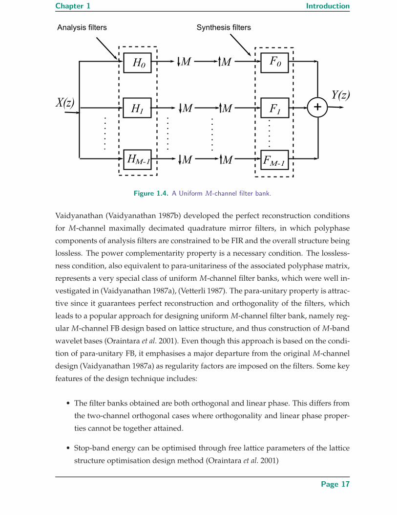
1.4 A Uniform M-channel filter bank. . . . . . . . . . . . . . . . . . . . . . . . 17
1.5 Non-uniform M-channel filter bank. . . . . . . . . . . . . . . . . . . . . . 19
1.6 Histograms of the sparsity measures . . . . . . . . . . . . . . . . . . . . . 20
1.7 RADWTs versus dyadic wavelet transforms frequency decomposition. . 21
2.1 Analysis M-channel NUFB (a) and the desired spectrum splitting (b). . . 27
2.2 Two-channel NUFB and the desired spectrum output . . . . . . . . . . . 28
2.3 Three-channel NUFB and the desired spectrum output . . . . . . . . . . 29
2.4 Three-channel NUFB and the required filters’ responses . . . . . . . . . . 31
2.5 Iterated rational two-channel filter bank on the analysis side . . . . . . . 32
2.6 j−stage iterated analysis low-pass filter and the equivalent structure . . 33
2.7 Shift variance in iterated RFB . . . . . . . . . . . . . . . . . . . . . . . . . 34
2.8 Orthogonal FIR RFB structure (Blu 1998) . . . . . . . . . . . . . . . . . . 36
2.9 Responses of literature design (Blu 1998) . . . . . . . . . . . . . . . . . . . 36
2.10 Responses of literature designs (Blu 1998) versus (Bayram and Selesnick
2009b) . . . . . . . . . . . . . . . . . . . . . . . . . . . . . . . . . . . . . . 37
2.11 Wavelet functions of the Fourier based designs (Auscher 1992) . . . . . . 38
2.12 Over-complete FIR rational FB structure of (Bayram and Selesnick 2009c) 40
2.13 Responses of literature design (Bayram and Selesnick 2009c) . . . . . . . 40
2.14 Over-complete IIR rational FB structure of (Bayram and Selesnick 2009a) 41
2.15 Tunable Q RFB structure (Selesnick 2011a) . . . . . . . . . . . . . . . . . . 42
3.1 RFB of ( q−1q , 1
q ) re-sampling rate structure . . . . . . . . . . . . . . . . . . 47
Page xvii
List of Figures
3.2 Rational rate filter bank with rate changing of (p0q ,
p1q ) for coprime pairs
(p0, q) and (p1, q) . . . . . . . . . . . . . . . . . . . . . . . . . . . . . . . . 48
3.3 Frequency responses of the polyphase components . . . . . . . . . . . . 58
3.4 Initialisation response of the nonlinear approach for RFB (4/5, 1/5) design 59
3.5 Comparison responses between the proposed approaches and literature
design (Blu 1998) . . . . . . . . . . . . . . . . . . . . . . . . . . . . . . . . 62
3.6 Comparison responses between the two proposed approaches . . . . . . 64
3.7 Comparison responses between the proposed approaches and literature
design (Blu 1998, Bayram and Selesnick 2009b) . . . . . . . . . . . . . . . 65
3.8 Father wavelet functions of example 5 (a), (b) and example 2b (c), (d). . . 66
4.1 Rational rate filter bank with rate changing of (p0q ,
p1q ) for coprime pairs
(p0, q) and (p1, q) . . . . . . . . . . . . . . . . . . . . . . . . . . . . . . . . 72
4.2 The equivalent RFB structure with the structure in Fig. 4.1 (a) . . . . . . 74
4.3 Analysis wavelet functions of various Q factor bi-orthogonal transforms 81
4.4 Synthesis wavelet functions of various Q factor bi-orthogonal transforms 81
4.5 Frequency response of RFB (47 , 3
7) - two regularity orders . . . . . . . . . 83
4.6 Frequency response of RFB ( 811 , 3
11) - two regularity orders . . . . . . . . 84
4.7 Frequency response of RFB (58 , 3
8) - three regularity orders . . . . . . . . 85
4.8 Frequency response of RFB ( 710 , 3
10) - three regularity orders . . . . . . . 85
4.9 Iterated (58 , 3
8) RFB - one/four regularity orders . . . . . . . . . . . . . . . 86
4.10 Low pass filters of (58 , 3
8) RFB - one/four regularity orders . . . . . . . . 87
4.11 Mean of the max absolute error . . . . . . . . . . . . . . . . . . . . . . . . 88
4.12 Frequency response of RFB ( 813 , 5
13) - one regularity order (modified iter-
ative approach) . . . . . . . . . . . . . . . . . . . . . . . . . . . . . . . . . 91
5.1 Plots of sparsity measure based on pq-mean . . . . . . . . . . . . . . . . . 97
5.2 Plots of sparsity measure based on pq-mean . . . . . . . . . . . . . . . . . 98
5.3 Histograms of the sparsity measures . . . . . . . . . . . . . . . . . . . . . 99
5.4 TIMIT speech denoising comparison . . . . . . . . . . . . . . . . . . . . . 100
Page xviii
List of Figures
5.5 TIMIT speech denoising gain histograms . . . . . . . . . . . . . . . . . . 101
5.6 Speech signal decomposition to low and high resonant components . . . 104
5.7 Chirp signal separation from narrow band interference (prolonged sinu-
soid) . . . . . . . . . . . . . . . . . . . . . . . . . . . . . . . . . . . . . . . 106
5.8 Spectrogram plot of interfered chirp signal . . . . . . . . . . . . . . . . . 107
5.9 Chirp signal separation from narrow band interference (short bursts) . . 108
5.10 Spectrogram plot of interfered chirp signal . . . . . . . . . . . . . . . . . 109
5.11 Spectrogram plot of interfered chirp signal . . . . . . . . . . . . . . . . . 110
5.12 Chirp signal separation from narrow band interference (short bursts at
band-pass region) . . . . . . . . . . . . . . . . . . . . . . . . . . . . . . . . 111
A.1 The filter H(z) and its frequency shifts magnitude response . . . . . . . 124
B.1 Iterated (23 , 1
3) RFB - two regularity orders . . . . . . . . . . . . . . . . . . 129
B.2 Iterated (34 , 1
4) RFB - two regularity orders . . . . . . . . . . . . . . . . . . 129
B.3 Iterated (67 , 1
7) RFB - two regularity orders . . . . . . . . . . . . . . . . . . 130
B.4 Iterated ( 910 , 1
10) RFB - three regularity orders . . . . . . . . . . . . . . . . 131
Page xix

Page xx

List of Tables
2.1 Approaches in the literature for the design of RFBs leading to RADWTs 44
3.1 Examples 1-5 designs’ parameters . . . . . . . . . . . . . . . . . . . . . . 61
3.2 Filters’ lengths comparison . . . . . . . . . . . . . . . . . . . . . . . . . . 68
4.1 The filter design parameters for the examples. . . . . . . . . . . . . . . . 84
5.1 SNR versus SIR for linear chirp and prolonged sinusoidal signals sepa-
ration . . . . . . . . . . . . . . . . . . . . . . . . . . . . . . . . . . . . . . . 107
5.2 Reconstructed SNR versus SIR for linear chirp and short burst sinusoid
separation . . . . . . . . . . . . . . . . . . . . . . . . . . . . . . . . . . . . 109
B.1 The filter design parameters for appendices B.1.1-B.1.4. . . . . . . . . . . 128
Page xxi

Page xxii

Chapter 1
Introduction
TIME-frequency analysis is an important tool in the field of signal
processing, especially for non-stationary signal analysis. A time-
frequency decomposition projects a time signal into a space which
facilitates detection (of events), filtering and classification (of phenomena).
In the new time-frequency space, the considered signal’s components of in-
terest can be well separated since such separation cannot be attained in the
original time domain. Hence, thresholding and some other well known ker-
nel methods can be applied for detection, filtering and classification tasks
once time-frequency analysis is used in extracting the signals’ features. This
chapter provides an introduction to the prominent time-frequency analysis
methods together with an outline of the thesis.
Page 1

1.1 Introduction
1.1 Introduction
Wavelet transform is a way of decomposing signals into a linear combination of wave-
forms which are scaled and shifted versions of a template signal. The coefficients
can be analysed or processed in manners appropriate to applications. The transform
provides good localisation in time and frequency at multiple resolutions in these do-
mains. The wavelet transform continuously trades off time resolution for frequency
resolution as the frequency changes, which differs from other time-frequency anal-
ysis such as short time Fourier transform (STFT). The short time Fourier transform
maintains constant time-frequency resolution for all frequencies, which is a contrast to
wavelet transform. The idea of wavelets was first developed in applied mathematics
and attracted great attention soon after across all fields including physics and engi-
neering. Wavelets hence can be approached from engineering perspective (sub-band
coding), physics (coherent states) and mathematics (study of Calderon-Zygmund op-
erators) (Daubechies 1992). The wavelet transforms, with a range of attractive fea-
tures such as multi-scale representations, piecewise smooth functions recovery, trans-
form flexibility, have become very successful in applications ranging from biomedi-
cal signal analysis (Unser and Aldroubi 1996), statistical analysis (Antoniadis 1997),
digital wireless communications (Lakshmanan and Nikookar 2006) and many others
(Sandercock et al. 2005, Pichot et al. 1999, Pichot et al. 2001, Belova et al. 2007).
For many years, dyadic wavelets and M-band wavelets (Daubechies 1992, Steffen et al.
1993) have been the most common, or conventional types. In the field of signal process-
ing, wavelet transform is well known for improving sparsity of signals’ representation,
defined as one in which small number of coefficients contain large majority of energy.
This property has been exploited by many applications, some classical examples are
de-noising (Pan et al. 1999) and classification (Ghinwa and James 2007, Farooq and
Datta 2001). Recently, sparse representation property has been further developed and
the uses range from signal separation (O’Grady et al. 2005, He et al. 2007), compression
(Goyal et al. 2008, Jiao et al. 2007, Blu et al. 2008), compressive sampling and signal anal-
ysis (Akcakaya and Tarokh 2008a). As a result, there have been interests in developing
a different way of representing signals, which departs from the conventional wavelets,
to further improve sparsity of representation.
In early 1990s non-uniform filter banks (NUFBs), which have non-integer re-sampling
ratios and unequal spectrum partitioning, have received much interest. One of the
Page 2
Chapter 1 Introduction
earliest works on this topic, presented by Kovacevic and Vetterli, addressed the is-
sues of perfect reconstruction for non-uniform FBs. The authors devised a generalised
feasibility test for perfect reconstruction (PR) conditions in a non-uniform FB struc-
ture and developed two methods of designing non-uniform FBs, namely direct and
indirect methods (Kovacevic and Vetterli 1993). A subsequent direction of research
explored the generalisation of the link between iterated two channel uniform FBs and
dyadic wavelets to the non-uniform case (Blu 1993). Iterated non-uniform FBs, or iter-
ated rational FBs (RFBs) with regularity factors can be viewed as approximate wavelet
transforms with rational dilation factors. Such a transform is named rational discrete
wavelet transform (RADWT), which is a weaker form of wavelet transform as they only
satisfy approximately the conditions for conventional wavelets (Blu 1998). The biggest
challenge for designing RADWTs is the issue of shift variance. The phenomenon refers
to the cases where the designed filter of a rational rate FB does not converge to a unique
wavelet function (Blu 1993), details of which will be discussed in chapter 2.
This thesis aims to advance the design of PR non-orthogonal critically-sampled RADWT
or bi-orthogonal RADWT which satisfy regularity conditions; either name will be used
interchangeably throughout the thesis. The FB is bi-orthogonal because in PR critically-
sampled FBs, the synthesis bank is the inverse of analysis bank and inverse matrices
automatically involve bi-orthogonality (Strang and Nguyen 1996). Specifically, there
are no works in the literature on the subject of designing bi-orthogonal RFB struc-
tures that we are aware of, let alone the iterated version. In this thesis, design chal-
lenges such as the issue of shift variance in RADWTs is addressed and results are pre-
sented. Three approaches to solving non-linear constraint optimisation are proposed
for the problem of designing bi-orthogonal rational FBs satisfying regularity condi-
tions. The resulting RADWTs provide constant Q-transforms as similar to the conven-
tional dyadic counterpart, where Q denotes the quality factor of the transform. This
quality factor Q is approximately two in dyadic wavelet transform and greater in
RADWT case. The ability to adjust Q flexibly can be useful in the analysis of many
oscillatory signals such as speech or EEG signals (Selesnick 2011a). This flexibility of Q
in RADWT and its applications are discussed in details in the thesis (chapter 4). Exper-
imental examples of sparse signal representation based on our proposed bi-orthogonal
RADWT are presented in chapter 5.
Page 3

1.2 Open questions to address
1.2 Open questions to address
To help understand the underlying role of bi-orthogonal RADWT in the family of
RADWTs and in the field of time-frequency analysis, this thesis will address the fol-
lowing questions
• The issue of shift-variance in constructing RADWT – how is it dealt with in bi-
orthogonal RADWT designs? What do we gain by relaxing orthogonality as
compared to RADWTs in existing literature?
• Bi-orthogonal rational filter bank design and the corresponding non-linear con-
straint optimisation – how is the resultant non-convex optimisation problem dealt
with?
• How is regularity order imposed on a bi-orthogonal rational filter bank structure?
• Which types of signals can benefit from our designed bi-orthogonal RADWTs
and which contexts can they be used in?
• In which context are constant Q transforms useful? What does flexibility of Q
value in constant Q transforms contribute?
• Why are dyadic/rational wavelet transforms necessary? What advantages can
they bring as compared to other time-frequency analysis techniques?
1.3 Overview of the thesis
The thesis is outlined as follows:
• In chapter 1, we present the outline of the thesis along with some background on
time frequency analysis, which ends with discussion on rational discrete wavelet
transform and their applications.
• Chapter 2 provides a review of the literature on this topic with the challenges for
constructing rational DWTs.
• In chapter 3, two channel ( q−1q , 1
q ) RFB and its corresponding wavelet is consid-
ered. Motivation for such choice of re-sampling parameters is briefly discussed.
Page 4

Chapter 1 Introduction
This chapter begins with the construction of the FB design problem into a non-
linear optimisation problem, then describes two solving methods and design re-
sults.
• In chapter 4, the general two channel ( pq ,
q−pq ) rate changing RFB and their corre-
sponding wavelets are discussed. Hence, flexible Q factor transform is enabled.
An iterative routine for solving the design problem in this case is considered and
design results are presented.
• Applications such as de-noising, signal separation based on l1 optimisation or
basis pursuit with bi-orthogonal RADWTs constructed dictionary are discussed
in chapter 5.
• Chapter 6 presents thesis conclusion and contains suggestions for potential fu-
ture work.
1.4 Background on Time-frequency analysis
Fourier transform has long been a fundamental tool for signal analysis whose applica-
tions vary across many fields and applications (Terras 1999, Folland 2009). The Fourier
transform expands signals into a basis formed by complex sinusoids, which form an
orthogonal basis. However, Fourier analysis has several notable shortcomings for the
analysis of non-stationary signals, most notably being the lack of time information in
the frequency representation. In other words, although all frequencies present in a
signal can be determined by Fourier analysis, their times of appearance are unknown.
Gibbs phenomenon, which refers to the appearance of overshoots in truncated Fourier
expansions when representing signals with discontinuities, is another issue in practice.
In analysing non-stationary signals, there is often strong interest in knowing when the
different frequency components occur. For example, as the time information of the sig-
nal in the transform is not represented, the Fourier transform requires a large number
of basis vector components to represent short pulse-like signals, which expands the
representation cost and raises processing requirements. In another example such as
music signals, notes of certain frequencies are heard for some finite interval of time
and they are then replaced by some other notes. Processing of these signals are not
usually interested in the overall contribution of the notes or frequencies but rather the
timing and duration of these notes. Hence, it is necessary to develop representation
Page 5
1.4 Background on Time-frequency analysis
schemes that contain both time and frequency information; such schemes are collec-
tively known as joint time-frequency representations.
Several time-frequency representations have been proposed and developed over the
past few decades such as Wigner-ville distribution (WVD) (Stankovic 1994, Kumar
and Prabhu 1997), short time Fourier transform (STFT) or windowed Fourier trans-
form (Kwok and Jones 2000, Rothwell et al. 1998, Durak and Arikan 2003), and wavelet
transform (Mallat 1989b).
In what follows, we provide a short discussion on short time Fourier analysis and
wavelet transform. The first technique is one of the earliest time-frequency represen-
tations, developed based on the classical Fourier analysis since Dennis Gabor sug-
gested to expand signals into a set of functions which are concentrated in both time
and frequency (Gabor 1946). Short Time Fourier transforms (STFTs) have since be-
come wide-spread in practice due to their computational simplicity (Liu 1993, Amin
and Feng 1995, Chen et al. 1993). The later technique, wavelet transform, is another
important time-frequency representation, which was originally proposed as time-scale
representation (Daubechies 1990, Mallat 1989b). This representation provides prop-
erties that could not be achieved in STFTs, details of which are discussed in section
1.4.2.
1.4.1 Short Time Fourier analysis
Short Time Fourier Transform is a signal decomposition technique that is designed
to overcome the aforementioned issues of purely time or frequency representations.
The STFT’s basis functions, defined as e−jωtw(t − τ), are modulated versions of a win-
dow function w(t) (Portnoff 1980). We can consider the transform as signal s(t) being
multiplied with the window function w(t), which is usually compactly supported, and
Fourier transform is then applied to the product w(t)s(t). The major advantage of such
transform is the decomposition localisation, which is suitable for input signals whose
energy is concentrated in certain regions of the time-frequency plane. The transform
coefficients will be near zero in other regions of the time-frequency plane and so con-
tain little energy; they can be computed as
cm,n =∫ +∞
−∞e−jmω0tw(t − nt0)s(t) dt (1.1)
Page 6

Chapter 1 Introduction
for parameters m, n ∈ Z and w(t) is called the window function or envelop function. The
coefficients {cm,n} of (1.1) represent the original signal s(t) in the new domain. How-
ever, one can question how completely and easily can the signal s(t) be reconstructed
from the set of coefficients cm,n and how well {cm,n} define s(t). The originally pro-
posed Gabor’s distribution, which is a special case of STFT with w(t) being chosen to
be Gaussian window without compact support and ω0t0 = 2π, leads to unstable re-
construction (Raab 1982). In other examples, if ω0t0 < 2π, reconstruction stability can
be attained and the time-frequency localisation properties of STFT became very useful
in many applications (Davis and Heller 1979).
In addressing the issue of reconstruction in STFT, Daubechies (Daubechies 1990) adopted
the analysis of coherent states, used in many areas of theoretical physics, which are de-
fined as
w(p,q)(x) = ejpxw(x − q), (1.2)
where the family of coherent states w(p,q)(x) are obtained by function w(x) being trans-
formed by p and translated by q. If the continuous parameters (p, q) in (1.2), which
determine the phase space setting of the coherent states w(p,q)(x), are discretised to re-
duce the transform’s redundancy as p = mp0, q = nq0 for m, n ∈ Z; p0, q0 > 0 and
p0q0 < 2π, the functions w(p,q)(x) will give rise to a frame for any function w(x) ∈L2(R) (Daubechies 1990). Hence, reconstruction stability is guaranteed; w(p,q)(x) can
be written as
w(m,n)(x) = ejp0mxw(x − q0n). (1.3)
If we let p0 = ω0, q0 = t0 and x equal to time t, we obtain the expression of STFT
in (1.1) and the reconstruction condition becomes ω0t0 < 2π and the transform is
referred to as over-sampling. If ω0t0 = 2π, the transform is critically-sampled (Qian and
Chen 1999), for which case w(.) is required to either not very smooth or it does not
decay very fast to attain a frame (Daubechies 1990). In order words, orthogonal basis
or critical-sampling transform can only be achieved with window function w(.) being
poorly localised. Hence, over-sampling STFT is often used to attain better behaved
window functions w(.) (Vetterli and Herley 1992).
Page 7

1.4 Background on Time-frequency analysis
Figure 1.1. Time-frequency plane of the short-time frequency analysis. Two different tilings are
shown, corresponding to different choices for windows and modulation frequencies.
Figure 1.2. Time-frequency plane of the dyadic wavelet transform. The frequency resolution is
much finer in low frequency and it corresponds to longer time basis function. At high
frequency, the time interval of the basis function is shorter; it corresponds to coarser
frequency resolution and better time resolution.
1.4.2 Wavelet transforms
One limitation of STFTs however is that, because a single window is used for all fre-
quencies, the resolution of the analysis is constant across the frequency axis as illus-
trated in the Fig. 1.1. Such constant resolution can be a disadvantage for STFTs, for ex-
ample when dealing with discontinuous signals. Such signal discontinuities can be ef-
fectively isolated by using transform of short-time, high-frequency and long-time, low-
frequency basis functions, which are the attributes of wavelet functions (Strang and
Nguyen 1996). Besides, wavelet functions with good time and frequency localisation
can be constructed even with critical sampling transform (Vetterli and Kovacevic 1995).
The wavelet basis functions are obtained from a single prototype wavelet by transla-
tion and dilation (Mallat 1989b), which are defined as
ψa,b(t) =1√a
ψ(t − b
a), (1.4)
Page 8
Chapter 1 Introduction
where a ∈ R+, b ∈ R; ψ(.) represents the mother wavelet function, which is required
to satisfy the admissibility condition
∫ +∞
−∞
|Ψ(ω)|2|ω| dω < ∞, (1.5)
where Ψ(ω) represents the Fourier Transform of ψ(t); 1.5 implies that
|Ψ(ω)|2ω=0 = 0, (1.6)
which results in wavelet spectrum being band-pass. It consequently implies that low
frequencies cannot be represented using wavelet functions. The father wavelet func-
tion is defined to complement the wavelet function (Mallat 1989b), as it neatly fits into
the low pass region of the spectrum that is left uncovered by wavelet functions. The
admissibility condition of father wavelet functions is stated as
∫ +∞
−∞φ(t)dt = 1. (1.7)
The discretised version of the wavelet function expression in (1.4) is defined as
ψm,n(t) = a−m/20 ψ(a−m
0 t − nb0) for m, n ∈ Z, (1.8)
which in this case, shows no absolute limitation for a0, b0 to constitute a frame, unlike
in STFT case which needs p0q0 ≤ 2π. In order words, a frame can be constituted
for any arbitrary pair of a0, b0. To take the argument further, it is also shown that for
arbitrary choices of a0 > 1, b0 > 0, tight frames can be constructed (Daubechies 1990).
For example, an orthogonal basis was constituted for a0 = 2, b0 = 1 (Meyer 1989). In
what follows, a very attractive attribute of wavelet transforms used in computer vision
and image processing, will be discussed.
1.4.2.1 Multi-resolution of wavelet transforms
The concept of multi-resolution analysis (MRA) was first introduced by Mallat (Mallat
1989b). In a MRA, let V0 be the space that is spanned by basis functions {φ0(t − k), k ∈Z}, defined as φ0(t) = φ(t) being the father wavelet function (i.e. b0 = 1). If a signal
f0(t) ∈ V0, it follows that f0(t) can be expanded as a linear combination of {φ0(t −k), k ∈ Z}. If we define Vj as the space spanned by {φj(t − k) = φ(a
j0t − k), k ∈ Z, a0 >
1}, then the scaled function f j(t) = f0(aj0t) is in Vj. MRA defines a nested sequence of
subspaces . . . , V−1, V0, V1, V2, . . . , Vj such that
. . . ⊂ V0 ⊂ V1 ⊂ . . . ⊂ Vj−1 ⊂ Vj . . . (1.9)
Page 9

1.4 Background on Time-frequency analysis
If Wj−1 is defined to be the orthogonal complement space of Vj−1 , then Vj is equivalent
to the “sum” of Vj−1 and Wj−1, defined as
Vj = Vj−1 ⊕ Wj−1. (1.10)
Physically, Wj−1 defines the detail of signal while Vj−1 defines the approximation of a
signal at level j− 1. Hence, (1.9) implies that the approximations at level j− 1, spanned
by {φj−1,k}k∈Z, combine with details at level j − 1, spanned by {ψj−1,k}k∈Z, to form the
approximation of the signal at the finer level j.
Another interpretation of f j(t) is the projection of the original function f (t) on the
subspace Vj and it is then said to be represented at the jth resolution level. The larger
the value of j, the finer its resolution. The signal’s projection onto Vj corresponds to a
time scale ∆t = a−j0 in the representation. Since f j(t) can be seen as an approximation
of the function f (t) on Vj, the error of such approximation can be shown to satisfy
(Strang and Nguyen 1996)
∥∥ f (t)− f j(t)
∥∥ ≈ C(∆t)p
∥∥∥ f (p)(t)
∥∥∥ , (1.11)
where p and constant C depends on the choice of wavelet functions (or filters of the
corresponding filter banks); ‖·‖ represents general Ln-norm operation since wavelets
are unconditional basis for function space Ln (Strang and Nguyen 1996); f (p)(t) repre-
sents the pth derivative of the function f (t) with respect to t. It is clear that piecewise
smooth functions are better approximated by wavelet basis compared to Fourier anal-
ysis. One important result of the multi-resolution analysis is if we apply successive
approximation recursively as shown in (1.9), the nested subspaces which include all
the details at all resolutions converge to L2(R) space when j → ∞. If we let a0 = 2, the
above result can be interpreted as: whenever there are sequence of spaces satisfying
MRA conditions, there exists an orthonormal basis for L2(R) defined as
ψm,n(t) = 2m2 ψ(2mt − n) for m, n ∈ Z, (1.12)
such that ψm,n(t) is the orthonormal basis for Wm, which is the orthogonal complement
space of Vm satisfying (1.10) (Vetterli and Kovacevic 1995). This contributes to one of
the techniques of constructing wavelets, namely construction of wavelets using Fourier
technique. The example wavelets constructed based on this technique include Meyer’s
wavelets and wavelets for spline spaces, discussed in (Vetterli and Kovacevic 1995).
Page 10

Chapter 1 Introduction
1.4.2.2 Wavelet transforms and Filter banks
One of the links between wavelet transform and signal processing was first recognised
by Daubechies and Mallat (Mallat 1989a, Daubechies 1988), whose result provides an
alternative for performing wavelet decompositions through filter bank analysis or sub-
band decomposition. Furthermore, the result suggests that wavelets are intimately
connected to the existing body of knowledge on filter banks. Thus, an alternative to
direct constructions as typified by the approach based on Fourier transform and MRA,
it is equally valid to start with discrete-time filters. The filters, if designed to satisfy
certain conditions, will lead to continuous-time wavelets when iterated.
In Fig. 1.3, a uniform two channel filter bank is shown. Typically, {HLP, FLP} are low-
pass filters while {HHP, FHP} are complementary high-pass filters. Such two channel
filter bank is known as critically sampled, since the down-sampling factors in both
channels are equal to the number of channels.
Figure 1.3. Critically sampled uniform two-channel filter bank. Left filters form the analysis bank,
while the right ones form the synthesis bank.
Perfect reconstruction (PR) condition is the most fundamental consideration in design-
ing filter banks. This condition requires the output signal y[n] to be a delayed version
of input signal x[n]. Thus, it is necessary to cancel aliasing and amplitude distortions
caused by re-sampling and filtering operations in the filter banks; PR conditions can
Page 11

1.4 Background on Time-frequency analysis
be defined in matrix form, namely alias component (AC) matrix, as
[
HLP(z) HHP(z)
HLP(−z) HHP(−z)
] [
FLP(z)
FHP(z)
]
=
[
2z−l
0
]
(1.13)
From (1.13), it can be observed that there are many possible sets of {HLP, HHP, FLP, FHP},
that satisfy the required PR conditions. A common design approach is to start with
imposing additional constraints on the filter set. Hence, for automatic aliasing cancel-
lation a set of relationships between analysis and synthesis filters is imposed. A classic
choice, as discussed in (Strang and Nguyen 1996), is
FLP(z) = HHP(−z) FHP(z) = −HLP(−z), (1.14)
which can be straightforward to verify as we substitute (1.14) into the aliasing cancella-
tion condition as
HLP(−z)FLP(z) + HHP(−z)FHP(z) = 0
⇒ HLP(−z)HHP(−z)− HHP(−z)HLP(−z) = 0, (1.15)
In addition, (1.14) can guarantee that designing high-pass filter HHP results in low-pass
filter FLP and similarly, designing low-pass filter HLP will lead to high-pass filter FHP.
Hence, the problem of designing PR filter banks reduces to designing filters HLP, HHP
that satisfy
HLP(z)HHP(−z)− HLP(−z)HHP(z) = 2z−l. (1.16)
Let P(z) = HLP(z)HHP(−z), (1.16) can be written as
P(z)− P(−z) = 2z−l (1.17)
and the problem of designing PR filter bank can thus be summarised as
1. Design half band filter P(z) that satisfies (1.17),
2. Factor P(z) into HLP(z), HHP(z) and find the corresponding FLP(z), FHP(z) using
(1.14).
The design in step 1 corresponds to many choices of {HLP, HHP}. Hence, further con-
straints can be imposed on the filter set {HLP, HHP} as Smith and Barnwell (Smith and
Page 12
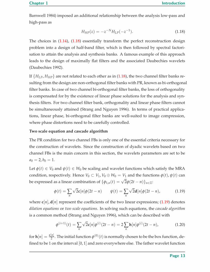
Chapter 1 Introduction
Barnwell 1984) imposed an additional relationship between the analysis low-pass and
high-pass as
HHP(z) = −z−N HLP(−z−1). (1.18)
The choices in (1.14), (1.18) essentially transform the perfect reconstruction design
problem into a design of half-band filter, which is then followed by spectral factori-
sation to attain the analysis and synthesis banks. A famous example of this approach
leads to the design of maximally flat filters and the associated Daubechies wavelets
(Daubechies 1992).
If {HLP, HHP} are not related to each other as in (1.18), the two channel filter banks re-
sulting from the design are non-orthogonal filter banks with PR, known as bi-orthogonal
filter banks. In case of two channel bi-orthogonal filter banks, the loss of orthogonality
is compensated for by the existence of linear phase solutions for the analysis and syn-
thesis filters. For two channel filter bank, orthogonality and linear phase filters cannot
be simultaneously attained (Strang and Nguyen 1996). In terms of practical applica-
tions, linear phase, bi-orthogonal filter banks are well-suited to image compression,
where phase distortions need to be carefully controlled.
Two scale equation and cascade algorithm
The PR condition for two channel FBs is only one of the essential criteria necessary for
the construction of wavelets. Since the construction of dyadic wavelets based on two
channel FBs is the main concern in this section, the wavelets parameters are set to be
a0 = 2, b0 = 1.
Let φ(t) ∈ V0 and ψ(t) ∈ W0 be scaling and wavelet functions which satisfy the MRA
condition, respectively. Hence V0 ⊂ V1, V0 ⊕ W0 = V1 and the functions φ(t), ψ(t) can
be expressed as a linear combination of {φ1,n(t) =√
2φ(2t − n)}n∈Z:
φ(t) = ∑n
√2c[n]φ(2t − n) ψ(t) = ∑
n
√2d[n]φ(2t − n), (1.19)
where c[n], d[n] represent the coefficients of the two linear expressions; (1.19) denotes
dilation equations or two scale equations. In solving such equations, the cascade algorithm
is a common method (Strang and Nguyen 1996), which can be described with
φ(i+1)(t) = ∑n
√2c[n]φ(i)(2t − n) = 2 ∑
n
h[n]φ(i)(2t − n), (1.20)
for h[n] = c[n]2 . The initial function φ(0)(t) is normally chosen to be the box function, de-
fined to be 1 on the interval [0, 1] and zero everywhere else. The father wavelet function
Page 13

1.4 Background on Time-frequency analysis
φ(t) is defined as φ(i)(t) → φ(t) as i → ∞, if the algorithm converges. In order words,
φ(t), ψ(t) exist only if the cascade algorithm (1.20) converges, which is determined by
h[n] or c[n] of (1.20) and the choice of function φ(0)(t). Moreover, when convergence
happens, it can be shown that (Vetterli and Kovacevic 1995) c[n], d[n] in the two scale
equations in (1.19) correspond to the impulse responses of the low-pass and high-pass
filters in an orthogonal two-channel filter bank. This is similar to the structure illus-
trated in 1.3 for {HLP, HHP, FLP, FHP} satisfying PR and orthogonal conditions. As a
result, c[n], d[n] can be considered as scaled impulse responses of HLP, HHP with a√
2
scaling, respectively. FLP, FHP can be obtained from the PR relationships, some exam-
ples are those described in (1.14), (1.16), and (1.18).
The regularity condition is required to guarantee that the cascade algorithm in (1.20)
converges and φ(i)(t) converges to a piecewise smooth function φ(t) in L2(R) as i → ∞.
If we consider cascade algorithm (1.20) in Fourier domain as
Φ(i+1)(ω) =(
∑n
h[n]e−jnω/2)Φ(i)(
ω
2) = H(
ω
2)Φ(i)(
ω
2), (1.21)
where Φ(i+1)(ω), Φ(i)(ω), H(ω) are Fourier transforms of φ(i+1)(t), φ(i)(t), h[n], re-
spectively; (1.21) provides the relationship between Φ(i)(ω) and Φ(i+1)(ω); thus we
can write Φ(i)(ω) in in terms of Φ(0)(ω) as
Φ(i)(ω) =[ i
∏n=1
H(ω
2n)]Φ(0)(
ω
2i). (1.22)
Hence, the convergence of φ(i)(t) → φ(t) of cascade algorithm in (1.20) is equivalent
to the Φ(i)(ω) approaches Φ(ω) as i → ∞. Such convergence depends on the behavior
of the product[
∏∞n=1 H( ω
2n )]Φ(0)(ω
2i ) of (1.22) or
Φ(ω) =[ ∞
∏n=1
H(ω
2n)]Φ(0)(0) (1.23)
as i → ∞. Daubechies (Daubechies 1988) proposed the necessary and sufficient condi-
tions for filter H(ω) for a well-behaved Φ(ω), which are
H(0) = 1, (1.24)
and H(ω) =(1 + ejω
2
)NR(ω), sup
ω∈[0,2π]
|R(ω)| < 2N−1. (1.25)
(1.24) is required since H( ω2∞ ) of the product sequence approaches H(0) and the prod-
uct will approach infinity at ω = 0 if such condition fails; (1.25) is known as the reg-
ularity condition. Such condition represents the smoothing part of the function as the
Page 14

Chapter 1 Introduction
product[
∏∞n=1 H( ω
2n )], for H(ω) satisfying (1.25), becomes
∞
∏n=1
(1 + ej ω2n
2
)N ∞
∏n=1
R(ω
2n) =
(sin(ω2 )
ω2
)N ∞
∏n=1
R(ω
2n). (1.26)
Hence, the RHS of (1.26) along with the bound condition on |R(ω)| described in (1.25)
guarantee that the product | ∏∞n=1 H( ω
2n )| in (1.23) is bounded above. Thus the corre-
sponding limi→∞ φ(i)(t) exists and converges to a point-wise continuous father wavelet
function φ(t) (Vetterli and Kovacevic 1995). The parameter N, namely regularity order,
of the regularity condition in (1.25) plays a critical role in the resulting wavelets. It
determines the smoothness of the resulting father wavelet function φ(t) and thus the
accuracy p, as defined in (1.11), of the approximation of piecewise functions based on
multi-resolution analysis.
Some dyadic wavelet examples based on two-channel FBs
The PR and regularity conditions discussed above are required for constructing dyadic
wavelets based on two-channel filter banks. In the literature, some famous examples
include
1. Daubechies wavelets (max-flat filters): In two-channel filter bank and dyadic wavelets,
max-flat (Daubechies) filters (Daubechies 1992) form an important family of fil-
ters that result in an outstanding wavelets family since the closed form solution
of the max-flat filter can be attained with respect to any N regularity orders being
imposed in the designed finite impulse response (FIR) filter with minimal length.
The key features of this family are:
(a) The unitariness of the polyphase matrix constructed from the filters
(b) FIR filters leading to wavelets of finite support
(c) Frequency response is maximally flat at ω = 0 and ω = π. This feature
is crucial since it determines the convergence, and maximises the regularity
order of the designed filter.
2. Bi-orthogonal wavelets and bi-orthogonal filter banks: The filter bank structure con-
sists of bi-orthogonal filters, thus bi-orthogonal wavelet is expected. In the or-
thogonal case, the synthesis wavelets are the same as analysis wavelets. In con-
trast, for the bi-orthogonal case if φ(t), ψ(t) are the analysis scaling and wavelet
functions, then there exist φ(t), ψ(t) for synthesis scaling and wavelet functions,
respectively. Some key features of this family include
Page 15

1.4 Background on Time-frequency analysis
(a) The orthogonal property of the filters’ polyphase matrix is relaxed. How-
ever, linear phase can be attained(Antonini et al. 1992). Note that linear
phase is not achievable for orthogonal filter banks.
(b) For any level j of MRA, if the analysis father wavelet functions {φj,k(t)}k∈Zand wavelet functions {ψj,k(t)}k∈Z span the subspaces Vj, Wj, then the syn-
thesis scaling and wavelet functions {φj,k(t)}k∈Z, {ψj,k(t)}k∈Z span the cor-
responding dual subspaces Vj, Wj, such that
Vj ⊥ Wj, Wj ⊥ Vj, (1.27)
Vj + Wj = Vj+1, Vj + Wj = Vj+1, (1.28)
in which the sums are direct sums but not orthogonal sums as in the orthogonal
case in (1.10). This implies that the bi-orthogonal wavelet series expansions are
x(t) =+∞
∑j=−∞
+∞
∑k=−∞
< x, ψj,k > ψj,k. (1.29)
1.4.3 Wavelet transforms based on uniform M-channel FBs
In wavelet transforms, signals are decomposed into channels that have equal band-
widths on logarithmic scale which leads to constant Q transform1. For example, in
dyadic wavelet, centre frequencies of the decomposed sub-bands are separated by
whole octaves. Thus, high frequency channel will have wide bandwidth while low fre-
quency has narrow bandwidth. However, it may be of interest to have narrow band-
width at high frequency which cannot be achieved with dyadic wavelet decomposi-
tions, especially when dealing with applications of input signals such as long narrow-
band RF signals. In such cases, M-band (M > 2) wavelet transform may be consid-
ered. The transform offers more energy compactness and it offers narrower sub-band
decomposition in high frequency components as compared to dyadic wavelet trans-
form. The construction of M-band wavelets, based on uniform M-channel filter bank,
is discussed in this section. This section does not include the mathematical derivations
of the construction of M-channel FB but the focus is on the historical development
of such FB design techniques and their features. This is used to help set the context
of the work in this thesis. The uniform M channel filter bank is illustrated in Fig.
1.4. M-channel filter banks have been extensively investigated. In an early paper,
1The parameter Q represent quality factor, defined as the ratio between centre frequency and the
bandwidth of the sub-band being considered
Page 16
Chapter 1 Introduction
Figure 1.4. A Uniform M-channel filter bank.
Vaidyanathan (Vaidyanathan 1987b) developed the perfect reconstruction conditions
for M-channel maximally decimated quadrature mirror filters, in which polyphase
components of analysis filters are constrained to be FIR and the overall structure being
lossless. The power complementarity property is a necessary condition. The lossless-
ness condition, also equivalent to para-unitariness of the associated polyphase matrix,
represents a very special class of uniform M-channel filter banks, which were well in-
vestigated in (Vaidyanathan 1987a), (Vetterli 1987). The para-unitary property is attrac-
tive since it guarantees perfect reconstruction and orthogonality of the filters, which
leads to a popular approach for designing uniform M-channel filter bank, namely reg-
ular M-channel FB design based on lattice structure, and thus construction of M-band
wavelet bases (Oraintara et al. 2001). Even though this approach is based on the condi-
tion of para-unitary FB, it emphasises a major departure from the original M-channel
design (Vaidyanathan 1987a) as regularity factors are imposed on the filters. Some key
features of the design technique includes:
• The filter banks obtained are both orthogonal and linear phase. This differs from
the two-channel orthogonal cases where orthogonality and linear phase proper-
ties cannot be together attained.
• Stop-band energy can be optimised through free lattice parameters of the lattice
structure optimisation design method (Oraintara et al. 2001)
Page 17

1.4 Background on Time-frequency analysis
• Only relatively low orders of regularity (at most two orders) can be imposed
in the published designs (Oraintara et al. 2001) since the imposing of regularity
conditions is transformed to conditions of lattice coefficients in the lattice struc-
ture. Such transform increases the complexity of the design, especially in cases
of higher order of regularity.
Steffen and Helller (Steffen et al. 1993) designed regular M-channel filter banks us-
ing a different approach. The design method was a generalisation of minimal length
K-regular two-band Daubechies to M-band case. The method is to impose the regu-
larity condition directly into the low-pass filter and then derive a general scheme for
a minimal length regular M-band wavelet bases. Band pass and high pass filters can
be obtained from low-pass filter by a Gram-Schimidt process (Chui. 1992). The major
departure from two-band wavelet design, in which high-pass channel can be uniquely
determined once low-pass filter is designed, is the greater freedom in choosing the
band-and high-pass filters that match the designed low-pass filter in M-band case.
The key features of this technique can be summarised as
• The regularity order can be imposed with mathematical exactness; the minimum
length low pass filters with arbitrary K-order regularity in the M-band wavelet is
analytically obtained (Steffen et al. 1993).
• The main disadvantage is of poor stop band attenuation when minimal length
designs are sought.
1.4.4 Rational rate filter banks (RFB) and rational discrete wavelets
Motivation of RFB or non-uniform FB (NUFB): Multi-rate digital signal processing
techniques are often used in the analysis of non-stationary signals, with applications
in fields such as speech and image compression and telecommunications. Historically,
the most common multi-rate systems use dyadic scaling of re-sampling rates, which
lead to sub-bands with centre frequencies separated by whole octaves. In many ap-
plications, however, it may be possible to obtain greater sparsity in the sub-band de-
composition for non-dyadic structures. The analysis of certain classes of signals, such
as natural speech, electrocardiographic (ECG) recordings and image textures, can ben-
efit from filter banks with rational re-sampling factors (Baussard et al. 2004, Yu and
White 2005, Yu and White 2006, Selesnick 2010, Ghinwa and James 2007, Selesnick
Page 18

Chapter 1 Introduction
2011c), where the sub-band bandwidths can be varied more gradually than in uniform
filter banks. For example, iterated rational filter banks with tuneable Q-factors have
recently been used to enhance sparsity in the representation of EEG and speech sig-
nals (Selesnick 2011c, Selesnick 2011a).
An M-channel non-uniform FB or rational rate FB is illustrated in Fig. 1.5. As similar to
the uniform counter part, let {N0, . . . , NM−1} denote analysis low-pass, band-pass and
high-pass filters while {S0, . . . , SM−1} denote synthesis low-pass, band-pass and high-
pass filters, respectively. The FB is critically-sampled, thus requiring the rate changing
parameters to satisfy ∑M−1i=0
piqi= 1; if ∑
M−1i=0
piqi> 1, the structure is over-complete.
Figure 1.5. Non-uniform M-channel filter bank.
Unlike uniform FB whereas the frequency spectrum is usually equally partitioned
amongst the FB channels, RFBs offer more flexible frequency partitioning. This can
be advantageous in analysing real world signals such as speech audio. For example, in
Fig. 1.6 a comparison between dyadic and rational dilation wavelets on speech signal
representation is illustrated. Sparsity measure of GINI index as discussed in (Hurley
and Rickard 2009) is used in which high value of GINI index denotes sparser represen-
tation. The experiment compares a 6/5 RADWT with other common dyadic wavelet
transforms such as Daubechies and bi-orthogonal wavelets in terms of speech signal
representation sparsity, details of which are discussed in section 5.2.1. The experi-
ment shows sparser representation obtained by using 6/5 RADWT as compared to the
dyadic counterpart since such RADWT can approximate the psychoacoustic bark scale
(Fastl and Zwicker 2007). Figure 1.6 shows that the sparsity measure resulted from the
Page 19
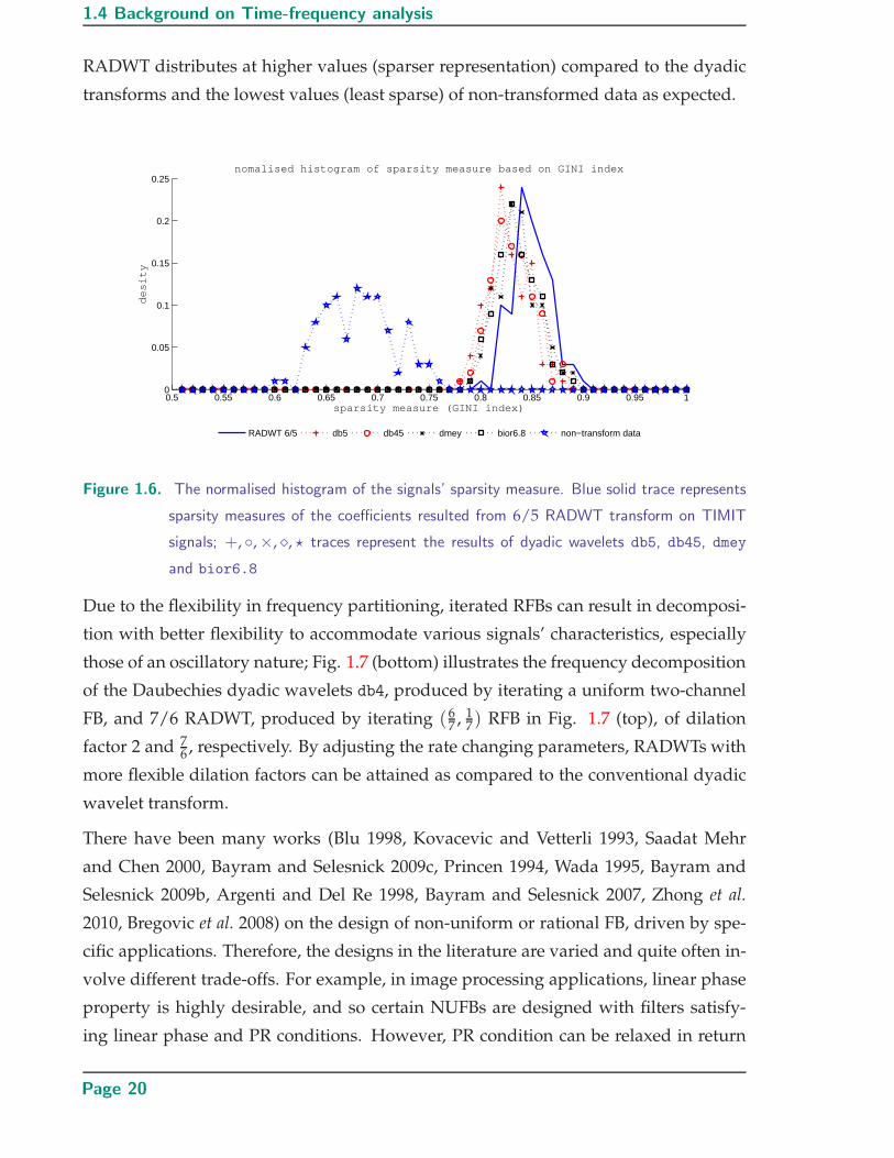
1.4 Background on Time-frequency analysis
RADWT distributes at higher values (sparser representation) compared to the dyadic
transforms and the lowest values (least sparse) of non-transformed data as expected.
0.5 0.55 0.6 0.65 0.7 0.75 0.8 0.85 0.9 0.95 10
0.05
0.1
0.15
0.2
0.25
sparsity measure (GINI index)
de
sity
nomalised histogram of sparsity measure based on GINI index
RADWT 6/5 db5 db45 dmey bior6.8 non−transform data
Figure 1.6. The normalised histogram of the signals’ sparsity measure. Blue solid trace represents
sparsity measures of the coefficients resulted from 6/5 RADWT transform on TIMIT
signals; +, ◦,×, �, ? traces represent the results of dyadic wavelets db5, db45, dmey
and bior6.8
Due to the flexibility in frequency partitioning, iterated RFBs can result in decomposi-
tion with better flexibility to accommodate various signals’ characteristics, especially
those of an oscillatory nature; Fig. 1.7 (bottom) illustrates the frequency decomposition
of the Daubechies dyadic wavelets db4, produced by iterating a uniform two-channel
FB, and 7/6 RADWT, produced by iterating (67 , 1
7) RFB in Fig. 1.7 (top), of dilation
factor 2 and 76 , respectively. By adjusting the rate changing parameters, RADWTs with
more flexible dilation factors can be attained as compared to the conventional dyadic
wavelet transform.
There have been many works (Blu 1998, Kovacevic and Vetterli 1993, Saadat Mehr
and Chen 2000, Bayram and Selesnick 2009c, Princen 1994, Wada 1995, Bayram and
Selesnick 2009b, Argenti and Del Re 1998, Bayram and Selesnick 2007, Zhong et al.
2010, Bregovic et al. 2008) on the design of non-uniform or rational FB, driven by spe-
cific applications. Therefore, the designs in the literature are varied and quite often in-
volve different trade-offs. For example, in image processing applications, linear phase
property is highly desirable, and so certain NUFBs are designed with filters satisfy-
ing linear phase and PR conditions. However, PR condition can be relaxed in return
Page 20
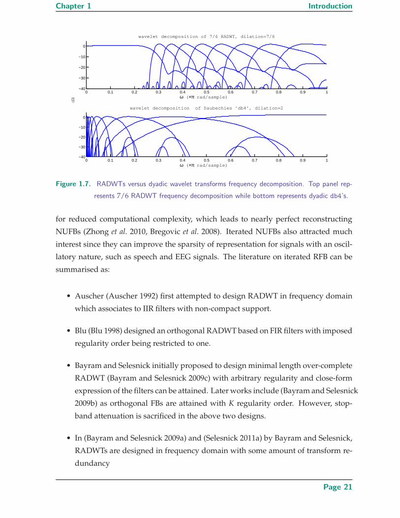
Chapter 1 Introduction
0 0.1 0.2 0.3 0.4 0.5 0.6 0.7 0.8 0.9 1−40
−30
−20
−10
0
wavelet decomposition of 7/6 RADWT, dilation=7/6
ω ( ×π rad/sample)
dB
0 0.1 0.2 0.3 0.4 0.5 0.6 0.7 0.8 0.9 1−40
−30
−20
−10
0
wavelet decomposition of Daubechies ’db4’, dilation=2
ω ( ×π rad/sample)
Figure 1.7. RADWTs versus dyadic wavelet transforms frequency decomposition. Top panel rep-
resents 7/6 RADWT frequency decomposition while bottom represents dyadic db4’s.
for reduced computational complexity, which leads to nearly perfect reconstructing
NUFBs (Zhong et al. 2010, Bregovic et al. 2008). Iterated NUFBs also attracted much
interest since they can improve the sparsity of representation for signals with an oscil-
latory nature, such as speech and EEG signals. The literature on iterated RFB can be
summarised as:
• Auscher (Auscher 1992) first attempted to design RADWT in frequency domain
which associates to IIR filters with non-compact support.
• Blu (Blu 1998) designed an orthogonal RADWT based on FIR filters with imposed
regularity order being restricted to one.
• Bayram and Selesnick initially proposed to design minimal length over-complete
RADWT (Bayram and Selesnick 2009c) with arbitrary regularity and close-form
expression of the filters can be attained. Later works include (Bayram and Selesnick
2009b) as orthogonal FBs are attained with K regularity order. However, stop-
band attenuation is sacrificed in the above two designs.
• In (Bayram and Selesnick 2009a) and (Selesnick 2011a) by Bayram and Selesnick,
RADWTs are designed in frequency domain with some amount of transform re-
dundancy
Page 21

1.5 Contributions and Publications
• In (Nguyen and Ng 2012, Nguyen and Ng 2010) and (Nguyen and Ng 2013), we
designed bi-orthogonal RADWTs based on FIR filters and with optimised stop-
band filters.
1.5 Contributions and Publications
The main contribution of this thesis include:
1. Design of two-channel bi-orthogonal rational FBs, with rational rate changes in
the two-channel satisfying (q−1
q , 1q ) (q ∈ N, q ≥ 3), which can lead to rational dis-
crete wavelet transforms. Arbitrary K regularity orders are imposed on the filters
which differentiates the proposed designs to those in the literature. Such a design
approach results in critically-sampled RADWT with adjustable smoothness and
offers better frequency resolution transform as compared to dyadic wavelets. This
comes from the fact that the designed rational dilation factor isq
q−1 < 2 for any
q ≥ 3. The rational re-sampling factors at the two channels are set to (q−1
q , 1q ) in
order to maximise the fine frequency decomposition when the FB is iterated for
a given value of q ≥ 3. The detailed design and two methods of solving the non-
linear constraint optimisation, arisen from the PR conditions of the FB structure,
is presented in chapter 3. Portions of this work has been published in
• NGUYEN-S., AND NG-B.-H. (2010). Critically sampled discrete wavelet
transforms with rational dilation factor of 3/2, Signal Processing (ICSP),
2010 IEEE 10th International Conference on, pp. 199 –202.
• NGUYEN-S. T. N., AND NG-B.-H. (2012). Design of two-band critically
sampled rational rate filter banks with multiple regularity orders and asso-
ciated discrete wavelet transforms, Signal Processing, IEEE Transactions on,
60(7), pp. 3863 –3868.
2. The adjustable Q factor transform is considered as the re-sampling rate param-
eters are generalised to (p0M ,
p1M ) for p0 + p1 = M and co-prime pairs p0, M and
p1, M . An iterative algorithm is proposed to solve the optimisation problem
arisen from this design. Generalised conditions for imposing regularity on the
RFB structure is discussed. This work will be covered in chapter 4, and some
parts of this appeared in
Page 22

Chapter 1 Introduction
• S. TRAN NGUYEN NGUYEN, AND B.W.-H.NG (2013). Bi-orthogonal ratio-
nal discrete wavelet transform with multiple regularity orders and applica-
tion experiments, Signal Processing (2013),
http://dx.doi.org/10.1016/j.sigpro.2013.04.001i.
3. The sparse representation of signals based on the proposed RADWTs is exploited.
We have shown that speech and chirp signals are amongst the signals which can
benefit from the designed bi-orthogonal RADWT. Chapter 5 will further discuss
on this topic. Parts of this work appears in
• S. TRAN NGUYEN NGUYEN, AND B.W.-H.NG (2013). Bi-orthogonal ratio-
nal discrete wavelet transform with multiple regularity orders and applica-
tion experiments, Signal Processing (2013),
http://dx.doi.org/10.1016/j.sigpro.2013.04.001i.
1.6 Chapter summary
This chapter provides fundamental and some historical background on time-frequency
analysis in which STFTs, wavelet transforms are amongst the known techniques. The
advantages of wavelet transform over STFTs are discussed. In the family of wavelets,
orthogonal, bi-orthogonal dyadic wavelets, M-band wavelets form the conventional
wavelets, which were thoroughly investigated by many authors from both mathematic
and signal processing perspectives. RADWTs, which are the main focus in this thesis,
have been developed more recently with the view to increase representation sparsity
over the conventional type wavelets for some types of signals. In that context, the
thesis outline and contributions are also presented in this chapter. A brief summary of
literature on M-band wavelets, rational DWTs is presented to emphasise the novelty of
the work presented in the thesis. In chapter 2, a detailed review of RADWT literature
will be presented.
Page 23

Page 24

Chapter 2
Iterated RFB - Designchallenges and literature
works
IN this chapter, the design challenges of iterated RFBs and RADWTs
are discussed. A summary on this topic’s literature is provided
with discussions on the key features of each technique. The litera-
ture review provides a framework that provides a suitable background for
the work described later in this thesis.
Page 25
2.1 Iterated rational filter bank designs - Design challenges
2.1 Iterated rational filter bank designs - Design chal-
lenges
There are two main issues associated with the design of iterated RFB. First, designing
perfect reconstruction (PR) filter banks with rational re-sampling factors is not straight-
forward. Unlike uniform FBs which do not suffer from aliasing if the filters are as-
sumed to have ideal brick wall responses, the non-integer re-sampling ratios in a RFB
structure can potentially produce aliasing which render PR impossible even with such
brick wall filters. A feasibility test to determine necessary conditions for perfect recon-
struction with respect to the rational re-sampling rates was established (Kovacevic and
Vetterli 1993). The second issue is specifically concerned with iterating RFB. The use
of rational re-sampling ratios in iterating FB leads to the issue of loss of shift invariance,
which was first discussed in (Blu 1993). Consequently, the translated father wavelet
functions {φj,k(t)}k∈Z will no longer constitute a basis or frame for Vj. Additionally,
the issue results in non-uniqueness of the limit function as the filters are iterated. In
practice, such design issue can be mitigated by strictly controlling the shift error, hence
it is critical for this to be constrained during the design process.
2.1.1 Aliasing in NUFBs structure – summary of necessary conditions
for PR non-uniform FB
A general analysis side M-channel RFB is illustrated in Fig. 2.1 (a) and the desired spec-
trum partitioning is shown in Fig. 2.1 (b). Let the analysis filters {N0, N1, . . . , NM−1}be real valued FIR filters with contiguous pass-band and the filter bank is critically-
sampled. Consider the the following examples:
Example 2.1.1. (aliasing of RFB): Let M = 2, p0 = 3, p1 = 2, q0 = q1 = 5, which corre-
sponds to a two channel RFB with rational re-sampling ratios (35 , 2
5). The structure is illus-
trated in Fig. 2.2 (a).
Let the channels with N0, N1 pick up low-pass spectra and high frequencies of the
input signal’s spectrum, respectively. If the input signal X(ω) is up-sampled by 2, the
resulting input spectrum X(2ω) will be compressed to the frequency band of [−π2 , π
2 ]
and periodic for every π. Hence to extract the expected high-pass spectrum of the
original signal, the filter N1 should have pass band response in the frequency bands
Page 26

Chapter 2 Iterated RFB - Design challenges and literature works
(a) M-channel NUFB
(b) NUFB M-channel spectra
Figure 2.1. Analysis M-channel NUFB (a) and the desired spectrum splitting (b).
[−π2 ,− 3π
10 ] and [ 3π10 , π
2 ] as illustrated in Fig. 2.2 (b). At the output of the filter, the signal
is down-sampled by 5. The positive half at frequency band [ 3π10 , π
2 ] is expanded to
[ 3π2 , 5π
2 ] as a result.
Consider the extracted negative band of the filter N1 output, as a result of down-
sampling operation by 5 the extracted frequency band is relocated at [−5π2 , −3π
2 ]. The
frequency band is equivalent to that at [−5π2 , −3π
2 ] + 2π= [ 3π2 , 5π
2 ]. However, the fre-
quency edge 3π2 corresponds to the original input spectrum at −π
2 which is at a higher
frequency component compared to that at 5π2 edge. Hence, the negative band results in
the extracted signal locating in frequency band of [ 3π2 , 5π
2 ], similar to the positive band,
Page 27

2.1 Iterated rational filter bank designs - Design challenges
(a) Analysis side of an ( 35 , 2
5 ) RFB structure
(b) ( 35 , 2
5 ) RFB desired band-pass response
Figure 2.2. Two-channel NUFB with rational rate changing ( 35 , 2
5)(a) and the desired spectrum at
the output of N1 filter (assumed ideal filter N1) (b).
however with reversed frequency order. Such overlapping renders perfect reconstruc-
tion impossible.
Note that if N1 is to extract signal occupying frequency bands ±[π2 , 7π
10 ], the similar
overlapping will occur at frequency region of [π2 , 3π
2 ], which again renders perfect re-
construction impossible.
Such aliasing in the high-pass response can be avoided for a slight adjustment in the
filter rate changing parameters. Consider the following example:
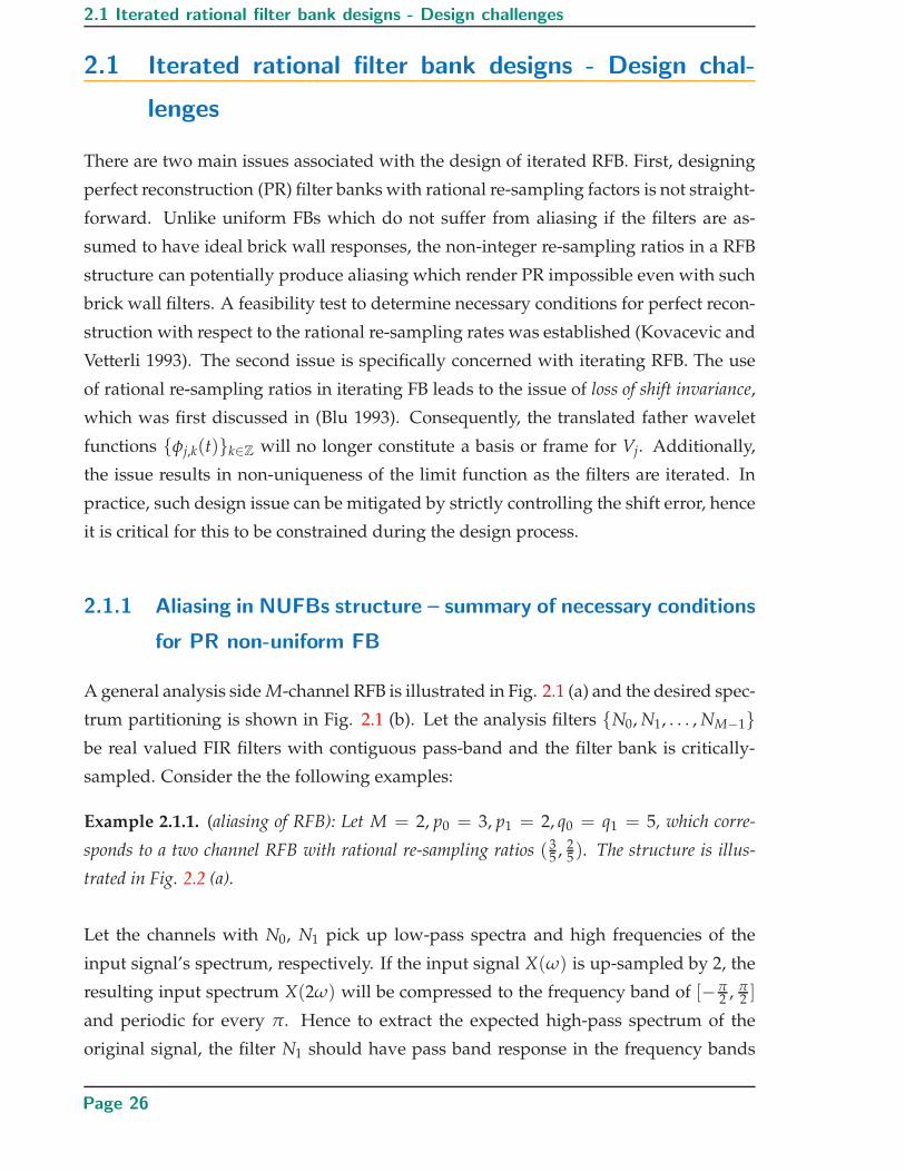
Example 2.1.2. Consider a three channel RFB with M = 3, p0 = 2, p1 = 2, p2 = 1 and
q0 = q1 = q2 = 5; the corresponding three channel RFB has rational re-sampling ratios of
(25 , 2
5 , 15). The structure is illustrated in Fig. 2.3
Page 28
Chapter 2 Iterated RFB - Design challenges and literature works
(a) 3-channel ( 25 , 2
5 , 15 ) RFB
(b) ( 25 , 2
5 , 15 ) RFB desired band-pass response
(c) Frequency response at the output of the down-sampling operation, i.e. I1
(d) Frequency response of Y1
Figure 2.3. (a) Three-channel NUFB with rational rate changing ( 25 , 2
5 , 15) and (b) the desired
spectrum at the output of N1 filter (assumed ideal band-pass filter N1); (c) illustrates
the response at I1 after the down-sampling operation while (d) represents the response
at Y1.
Consider the band-pass filter N1 of structure Fig. 2.3 (a). The extracted frequency
band is ±[− 2π5 ,−π
5 ]. We denote N and P for negative and positive bands of the con-
sidered real filter as shown in Fig. 2.3 (b). Note that up-sampling of input signal by
Page 29

2.1 Iterated rational filter bank designs - Design challenges
two resulting in the original extracted band-pass frequency bands at ±[ 2π5 , 4π
5 ] being
compressed to the [− 2π5 ,−π
5 ] and [π5 , 2π
5 ], hence the required band of filter N1. Since
down-sampling by 5 results in the signal’s spectrum being expanded by 5, the P and
N frequency bands at the N1 filter output are expanded to [π, 2π] and [0, π], respec-
tively. Note that 2π shifting has been done to the resulting frequency bands to bring
them within the fundamental Nyquist’s zone [−π, π]. This is illustrated in Fig. 2.3
(c). At this stage, no aliasing has occurred for this structure. Fig. 2.3 (d) illustrates the
response Y1 after up-sampling operation. If S1 has similar frequency response as N1,
the frequency bands as similar to those at the output of N1 will be extracted and the
order of positive and negative frequency bands are also picked up correctly. Hence, no
aliasing occurs in this case.
Note that for the low-pass channel (corresponding to filters N0, S0), in which the ex-
tracted frequency band of interest is in [−π5 , π
5 ], there is no aliasing caused by the
down-sampling operation by 5. In the high-pass channel (corresponding to filters
N2, S2), the extracted frequency bands are ±[ 4π5 , π]. Down-sampling by 5 results in
the bands being relocated to frequency regions of [0, π] and [−π, 0], for positive and
negative frequency bands, respectively. Similarly, as a result of the up-sampling 5, the
response is compressed by 5 in a similar manner but in a reverse P and N order of that
in Fig. 2.3 (d). These can be correctly reconstructed again if S2 has the same response
as N2.
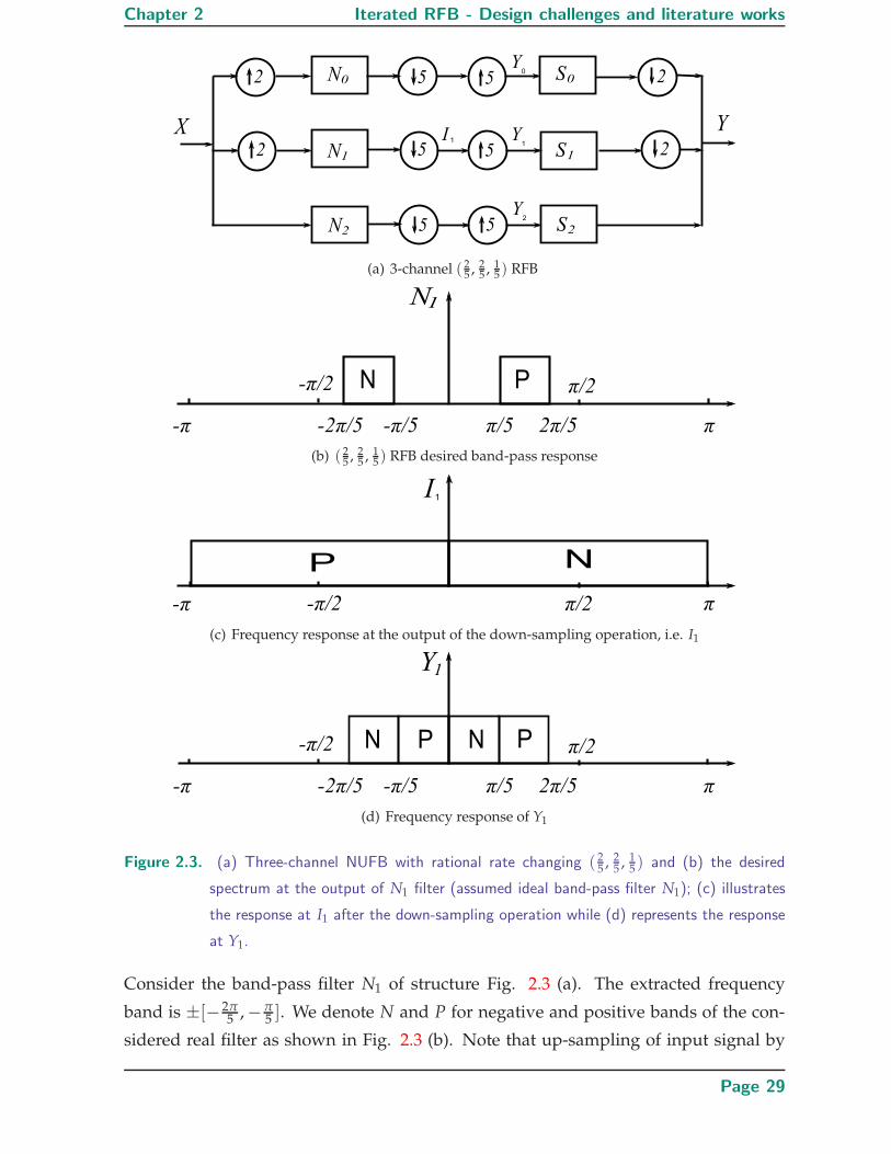
In summary, it is possible for a critically-sampled M-channel RFB structure with real
filters, to extract in the following frequency bands of input signal (Kovacevic and
Vetterli 1993) for any channel i = 0 . . . , M − 1:
Xi :[k
qπ,
k + p
qπ]
(2.1)
if there exist l, s such that one of the following pairs of conditions is satisfied,
k = sp − lq, l = 2t, (2.2)
k − q = lq − sp, l = 2t + 1, (2.3)
where l = 0, . . . , p − 1; s = 0, . . . , q − 1; and k = 0, . . . , q − p. If the solution exists for
(2.2) or (2.3), then the filters are required to have pass-bands
Ni, Si :[ s
q,
s + 1
q
]
. (2.4)
Page 30
Chapter 2 Iterated RFB - Design challenges and literature works
In example 2.1.1, extracting the spectrum from [ 310 π, 5
10 π] in channel 1 (i.e. i = 1) gives
k = 3, q = 10, p = 2. It can be verified that there exists no l ∈ [0, p − 1], s ∈ [0, q − 1]
that satisfy either (2.2) or (2.3).
In example 2.1.2, the following solutions of s, l can be found
• For low-pass channel consisting of S0, N0, the interested spectrum to be extracted
is [0, π5 ], hence k = 0, q = 5, p = 1 and the corresponding solution for (2.2) are
s = 0, l = 0.
• For band-pass channel consisting of S1, N1, the extracted spectrum is [π5 , 2π
5 ],
hence k = 1, q = 5, p = 1 and the corresponding solution for (2.2) are s = 1, l = 0.
• For high-pass channel with S2, N2, the spectrum of interest to be extracted is
[ 4π5 , π], hence k = 4, q = 5, p = 1 and the corresponding solution for (2.2) are
s = 4, l = 0.
The required frequency responses of the filters are illustrated in Fig. 2.4.
Figure 2.4. Three-channel NUFB with rational rate changing ( 25 , 2
5 , 15) and the required filters’
frequency responses; N0, N1, N2 represent low-pass, band-pass and high-pass filters, re-
spectively. Note that S0, S1, S2 are required to have the same responses of the illustrated
N0, N1, N2, respectively.
2.1.2 The issue of shift variance in iterated RFB
In iterated RFBs, the term shift-variance takes on a different meaning to the dyadic case.
For dyadic wavelet transform this term refers to the high dependence of wavelet co-
efficients on the time of appearance of the input signal. Delays in the input signal
can cause significant changes in the wavelet coefficients, which is caused by the sub-
sampling operation by 2 in dyadic discrete wavelet decompositions. In RADWTs, the
Page 31
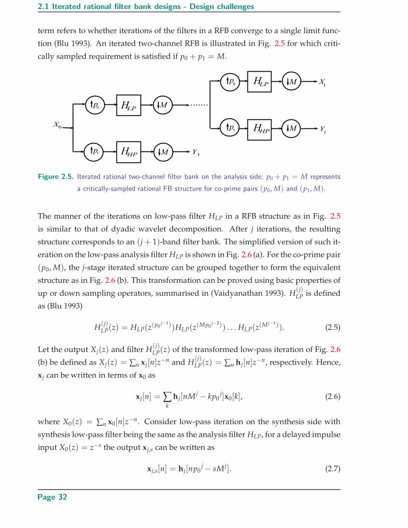
2.1 Iterated rational filter bank designs - Design challenges
term refers to whether iterations of the filters in a RFB converge to a single limit func-
tion (Blu 1993). An iterated two-channel RFB is illustrated in Fig. 2.5 for which criti-
cally sampled requirement is satisfied if p0 + p1 = M.
Figure 2.5. Iterated rational two-channel filter bank on the analysis side; p0 + p1 = M represents
a critically-sampled rational FB structure for co-prime pairs (p0, M) and (p1, M).
The manner of the iterations on low-pass filter HLP in a RFB structure as in Fig. 2.5
is similar to that of dyadic wavelet decomposition. After j iterations, the resulting
structure corresponds to an (j + 1)-band filter bank. The simplified version of such it-
eration on the low-pass analysis filter HLP is shown in Fig. 2.6 (a). For the co-prime pair
(p0, M), the j-stage iterated structure can be grouped together to form the equivalent
structure as in Fig. 2.6 (b). This transformation can be proved using basic properties of
up or down sampling operators, summarised in (Vaidyanathan 1993). H(j)LP is defined
as (Blu 1993)
H(j)LP(z) = HLP(z
(p0j−1))HLP(z
(Mp0j−2)) . . . HLP(z
(Mj−1)). (2.5)
Let the output Xj(z) and filter H(j)LP(z) of the transformed low-pass iteration of Fig. 2.6
(b) be defined as Xj(z) = ∑n xj[n]z−n and H
(j)LP(z) = ∑n hj[n]z
−n, respectively. Hence,
xj can be written in terms of x0 as
xj[n] = ∑k
hj[nMj − kp0j]x0[k], (2.6)
where X0(z) = ∑n x0[n]z−n. Consider low-pass iteration on the synthesis side with
synthesis low-pass filter being the same as the analysis filter HLP, for a delayed impulse
input X0(z) = z−s the output xj,s can be written as
xj,s[n] = hj[np0j − sMj]. (2.7)
Page 32
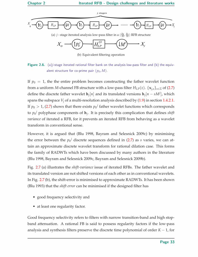
Chapter 2 Iterated RFB - Design challenges and literature works
(a) j−stage iterated analysis low-pass filter in a (p0M ,
p1M ) RFB structure
(b) Equivalent filtering operation
Figure 2.6. (a)j-stage iterated rational filter bank on the analysis low-pass filter and (b) the equiv-
alent structure for co-prime pair (p0, M).
If p0 = 1, the the entire problem becomes constructing the father wavelet function
from a uniform M-channel FB structure with a low-pass filter HLP(z). {xj,s}s∈Z of (2.7)
define the discrete father wavelet hj[n] and its translated versions hj[n − sMj], which
spans the subspace Vj of a multi-resolution analysis described by (1.9) in section 1.4.2.1.
If p0 > 1, (2.7) shows that there exists p0j father wavelet functions which corresponds
to p0j polyphase components of hj. It is precisely this complication that defines shift
variance of iterated a RFB, for it prevents an iterated RFB from behaving as a wavelet
transform in conventional sense.
However, it is argued that (Blu 1998, Bayram and Selesnick 2009c) by minimising
the error between the p0j discrete sequences defined in (2.7) as s varies, we can at-
tain an approximate discrete wavelet transform for rational dilation case. This forms
the family of RADWTs which have been discussed by many authors in the literature
(Blu 1998, Bayram and Selesnick 2009c, Bayram and Selesnick 2009b).
Fig. 2.7 (a) illustrates the shift-variance issue of iterated RFBs. The father wavelet and
its translated version are not shifted versions of each other as in conventional wavelets.
In Fig. 2.7 (b), the shift-error is minimised to approximate RADWTs. It has been shown
(Blu 1993) that the shift error can be minimised if the designed filter has
• good frequency selectivity and
• at least one regularity factor.
Good frequency selectivity refers to filters with narrow transition-band and high stop-
band attenuation. A rational FB is said to possess regularity factors if the low-pass
analysis and synthesis filters preserve the discrete time polynomial of order K − 1, for
Page 33

2.2 Existing Design approaches in the literature
0 1 2 3 4 5 6
−0.2
0
0.2
0.4
0.6
0.8
1
father wavelet functions (rational dilation factor)
(a)
28 30 32 34 36 38−0.1
0
0.1
0.2
0.3
0.4
0.5
(b)
33.7 33.8 33.9 34 34.1−0.09
−0.08
−0.07
father wavelet translated father wavelet
Figure 2.7. (a) iterated rational FB on the low-pass filter and its translated version (without min-
imising shift-error) (b) iterated rational FB and its translated version on the same interval
(with shift-error being minimised).
which K represents the regularity order. Simultaneously, the analysis high-pass channel
annihilates the discrete time polynomial of order K − 1. Thus, for rational FBs as in Fig.
2.5, the analysis low-pass and high-pass filters possess K regularity order if and only if
they satisfy the following conditions (Bayram and Selesnick 2009c, Steffen et al. 1993)
HLP(z) = (1 + z−1 + . . . + z−(p0−1))KP0(z), (2.8)
HHP(z) = (1 − z−1)KQ(z), (2.9)
and the synthesis low-pass filter is required to be divisible by
(1 + z−1 + . . . + z−(M−1))K. (2.10)
2.2 Existing Design approaches in the literature
The topic of designing rational filter banks has been addressed by many authors (Blu
1998, Kovacevic and Vetterli 1993, Saadat Mehr and Chen 2000, Bayram and Selesnick
2009c, Princen 1994, Wada 1995, Bayram and Selesnick 2009b, Argenti and Del Re 1998,
Bayram and Selesnick 2007). In that context, several approaches have attempted to im-
pose regularity orders on the design of RFB (Bayram and Selesnick 2007, Bayram and
Selesnick 2009b, Bayram and Selesnick 2009c, Bayram and Selesnick 2009a, Blu 1998).
Page 34

Chapter 2 Iterated RFB - Design challenges and literature works
Among these designs, Bayram and Selesnick (Bayram and Selesnick 2009b) attained K-
regular RFB with finite impulse response (FIR) filters in an orthonormal structure using
matrix factorisation, but this approach did not explicitly address the shift-variance is-
sue and hence frequency selectivity as reported in other papers on rational DWT (Blu
1993, Blu 1998, Bayram and Selesnick 2009c, Bayram and Selesnick 2009a). Further-
more, the design leads to near PR when K regularity orders are imposed on the FB
structure.
Bayram’s other designs (Bayram and Selesnick 2007, Bayram and Selesnick 2009c, Bayram
and Selesnick 2009a) are over-complete RFBs with arbitrary K regularity orders, and
the associated expansive decompositions can be undesirable for applications such as
signal compression. Blu’s design from an iterative optimisation algorithm resulted in
orthonormal RFBs which were approximately shift-invariant, although this algorithm
is reported to diverge for regularity orders greater than one (Blu 1998).
In this section, iterated RFB designs in the literature are presented and discussed. The
summary of the designs’ key features are separated into classes. This classification
is based on 1) redundancy of the eventual filter banks and 2) compactness of filter
support which can either be compact (FIR) and non-compact (IIR).
2.2.1 Critically sampled RFBs and RADWTs
Orthogonal RADWTs with compact support
One of the earliest approaches on RADWTs is presented in (Blu 1998), in which the
resultant design approximates rational DWT and satisfies PR, possesses regularity fac-
tors and are orthogonal. The FB consists of FIR filters, which are designed based on
an iterative algorithm. The designed filters are frequency selective and their iterations
lead to wavelet functions which are approximately shift-invariant. The FB structure is
shown in Fig. 2.8. The filters H(z), G(z) represent analysis low-pass and high-pass fil-
ters, respectively. The synthesis filters are time-reversed versions of the analysis filters.
Some key features of such designs include:
• the design algorithm is recursive and consists of a sequence of convex optimi-
sation routines. At each iteration, the low-pass filter’s stop band energy is opti-
mised against some linear constraints;
Page 35
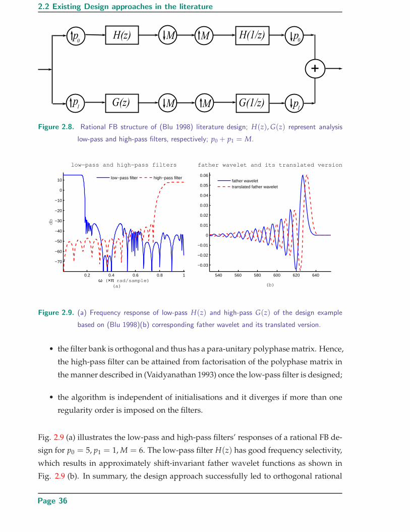
2.2 Existing Design approaches in the literature
Figure 2.8. Rational FB structure of (Blu 1998) literature design; H(z), G(z) represent analysis
low-pass and high-pass filters, respectively; p0 + p1 = M.
0.2 0.4 0.6 0.8 1
−70
−60
−50
−40
−30
−20
−10
0
10
low−pass and high−pass filters
db
ω ( ×π rad/sample) (a)
540 560 580 600 620 640
−0.03
−0.02
−0.01
0
0.01
0.02
0.03
0.04
0.05
0.06
father wavelet and its translated version
(b)
low−pass filter high−pass filter
father wavelettranslated father wavelet
Figure 2.9. (a) Frequency response of low-pass H(z) and high-pass G(z) of the design example
based on (Blu 1998)(b) corresponding father wavelet and its translated version.
• the filter bank is orthogonal and thus has a para-unitary polyphase matrix. Hence,
the high-pass filter can be attained from factorisation of the polyphase matrix in
the manner described in (Vaidyanathan 1993) once the low-pass filter is designed;
• the algorithm is independent of initialisations and it diverges if more than one
regularity order is imposed on the filters.
Fig. 2.9 (a) illustrates the low-pass and high-pass filters’ responses of a rational FB de-
sign for p0 = 5, p1 = 1, M = 6. The low-pass filter H(z) has good frequency selectivity,
which results in approximately shift-invariant father wavelet functions as shown in
Fig. 2.9 (b). In summary, the design approach successfully led to orthogonal rational
Page 36

Chapter 2 Iterated RFB - Design challenges and literature works
FBs with good frequency selectivity and possessing regularity orders. However, the
convergence of this approach is limited to filters with one regularity order.
In an attempt to overcome the limitation of only one regularity order, an algorithm
was proposed (Bayram and Selesnick 2009b) to design orthogonal rational FB with
arbitrary regularity orders. In this approach, the rational rate filter bank is decomposed
into the equivalent uniform filter bank, whose filters from each analysis and synthesis
side are DFT-modulated versions of each others. The approach shows poorer stop-
band performance as compared to (Blu 1998), provided the total length of filters are
similar. More importantly, the algorithm’s output does depend on the initialisation of
the design algorithm and the resultant FB only satisfies PR condition approximately,
i.e. only near PR filter banks. A comparison between the two filters resulted from the
two algorithms is shown in Fig. 2.10.
0 0.1 0.2 0.3 0.4 0.5 0.6 0.7 0.8 0.9 1−160
−140
−120
−100
−80
−60
−40
−20
0
low−pass filters
dB
ω ( ×π rad/sample)
(Blu 1998) design(Bayram and Selesnick 2009b) design
Figure 2.10. Blue solid trace represents Blu’s design (Blu 1998) (one regularity order) while red
dashed trace represents design in (Bayram and Selesnick 2009b) (two regularity orders);
FB rate changing factors are ( 56 , 1
6)
Orthogonal RADWTs with non-compact support
Auscher (Auscher 1992) first attempted to construct RADWTs in the Fourier domain,
which leads to non-compact support wavelet functions. For a rational dilation factor,
defined by a ratiopq for p, q ∈ N, p = q + 1, let function χ(ω) be an even function in
Page 37
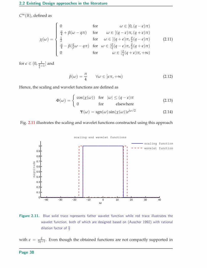
2.2 Existing Design approaches in the literature
C∞(R), defined as
χ(ω) =
0 for ω ∈ [0, (q − ε)π)π4 + β(ω − qπ) for ω ∈ [(q − ε)π, (q + ε)π)12 for ω ∈ [(q + ε)π,
pq (q − ε)π)
π4 − β(
qp ω − qπ) for ω ∈ [
pq (q − ε)π,
pq (q + ε)π)
0 for ω ∈ [ pq (q + ε)π,+∞)
(2.11)
for ε ∈ (0, 1pq +1
] and
β(ω) =π
4∀ω ∈ [επ,+∞) (2.12)
Hence, the scaling and wavelet functions are defined as
Φ(ω) =
{
cos(χ(ω)) for |ω| ≤ (q − ε)π
0 for elsewhere(2.13)
Ψ(ω) = sgn(ω) sin(χ(ω))ejω/2 (2.14)
Fig. 2.11 illustrates the scaling and wavelet functions constructed using this approach
−40 −30 −20 −10 0 10 20 30 400
0.1
0.2
0.3
0.4
0.5
0.6
0.7
0.8
0.9
1
scaling and wavelet functions
ω
ma
gn
itud
e
scaling function
wavelet function
Figure 2.11. Blue solid trace represents father wavelet function while red trace illustrates the
wavelet function, both of which are designed based on (Auscher 1992) with rational
dilation factor of 65
with ε =q
2q+1 . Even though the obtained functions are not compactly supported in
Page 38

Chapter 2 Iterated RFB - Design challenges and literature works
time, the design approach leads to a MRA with rational dilation factorpq . The designed
wavelet functions have shown to possess infinite number of regularity orders since the
frequency responses are precisely zero in all stop-band regions.
In summary, FIR based design offers compact support to the resulting wavelet func-
tions even though the obtained RADWTs only satisfy shift invariance approximately.
On the other hand, if the wavelet functions are constructed in Fourier domain, a MRA
with rational scaling factors can be obtained at the expense of needing infinite impulse
response (IIR) filters.
2.2.2 Overcomplete RFB – redundant RADWTs
Redundant 2 RADWTs with compact support
The topic of over-complete DWT with rational dilation factor was first addressed by
Bayram and Selesnick in (Bayram and Selesnick 2009c), whose filters are designed to
possess the following properties
• perfect reconstruction;
• self inverting FIR filters and compact support of basis functions;
• high-pass filters are designed based on matrix spectral factorisation;
• possess arbitrary number of (K) regularity orders with minimal length filters and
closed form solutions for low-pass filters, hence mathematical exactness;
• for a RADWT design with rational dilation factor of Mp0
for p0, M ∈ N, the redun-
dancy factor of the transform is alwaysp0+M
M .
The rational FB structure is illustrated in Fig. 2.12, in which H(z), Gn(z), n = 0, . . . , M−2 represent the low-pass and high-pass analysis filters, respectively. The synthesis fil-
ters are time-reversed versions of the analysis filters. Consider the following example,
in which a rational FB with p0 = 2, M = 3 and K = 4 regularity orders is designed
based on (Bayram and Selesnick 2009c). The filters are shown in Fig. 2.13. In Fig. 2.13
(a), only the response of G0(z) high-pass filter is shown since G1(z), G2(z) have very
2In this section, the terms over-complete and redundant are used interchangeably to denote RADWTs
with some redundancy.
Page 39

2.2 Existing Design approaches in the literature
Figure 2.12. Rational FB structure of (Bayram and Selesnick 2009c) literature design; H(z), Gn(z),
n = 0, . . . , M − 2 represent high-pass and low-pass filters, respectively.
0.2 0.4 0.6 0.8 1
−120
−100
−80
−60
−40
−20
0
ω ( ×π rad/sample)(a)
dB
low−pass and high−pass responses
100 150 200 250 300 350
0
5
10
15
20
x 10−3
father wavelet and its translated version
(b)
low−pass response
high−pass response
father wavelet
translated father wavelet
Figure 2.13. (a) Frequency response of low-pass H(z) and high-pass G0(z) of the design example
based on (Bayram and Selesnick 2009c) and (b) corresponding father wavelet and its
translated version.
similar frequency responses. The frequency response for low-pass filter H(z) is shown
with good stop band attenuation. Its regularity property is illustrated as H(ω) has ze-
ros at (ω = 2π/3, π), which corresponds to conditions (2.8), (2.10) for M = 3, p0 = 2.
The filter H(ω) is required to satisfy both (2.8), (2.10) for analysis and synthesis filters
since the previous filter is time-reversed version of the latter. The filter G0(z) is also
shown, from Fig. 2.13 (a) to have zeros at ω = 0 as a result of (2.9). Fig.2.13 (b) shows
the iterated low-pass filter or discrete father wavelet and the translated version, which
approximates the shifted version of the father wavelet function.
Page 40

Chapter 2 Iterated RFB - Design challenges and literature works
Figure 2.14. Rational FB structure of (Bayram and Selesnick 2009a) literature design; H(ω), G(ω)
represent low-pass and high-pass filters, respectively.
One notable disadvantage of the design lies in the pass-band region of the low-pass
filter, which is required to pass frequencies in the region [0, π3 ]. In this design, no opti-
misation is imposed on the frequency characteristic of the resulting filter at the expense
of minimal length filters and exact closed form formula. This leads to filters with poor
pass-band and transition-band responses as illustrated in Fig. 2.13(a).
Redundant RADWTs in Fourier domain (non-compact support wavelet functions)
Blu (Blu 1993) found that the construction of wavelet transform with rational dilation
factors can only be approximately attained with FIR filters since the resulting wavelet
functions are not perfectly shifted versions of each other. Hence, multi-resolution
analysis cannot be achieved perfectly for rational dilation factors. However, Auscher
(Auscher 1992) showed that MRA is achievable even in rational dilation cases if the the
wavelet functions are to be designed in Fourier domain, implying IIR filters. Bayram
and Selesnick extended the design idea, and allowed some degree of transform re-
dundancy (Bayram and Selesnick 2009a). The approach, which leads to RADWTs
and MRA with rational dilation factor, is constructed based on a single band-limited
filter. The allowed redundancy can be adjusted to provide adjustable Q-factor 3 of
the RADWT. This shows an improvement as compared to the approach in (Bayram
and Selesnick 2009c). Fig. 2.14 illustrates the design FB structure and its parameters
p, M, s, which determine the transform’s Q factor and its redundancy. For integer val-
ues p, M, s, the quality factor Q and the redundancy factor r of transform, is defined as
(Bayram and Selesnick 2009a)
Q =
√p
M
1
1 − pM
and r =1
s
1
1 − pM
(2.15)
3The quality factor Q factor is defined to be the ratio of centre frequency and the spectrum’s band-
width.
Page 41
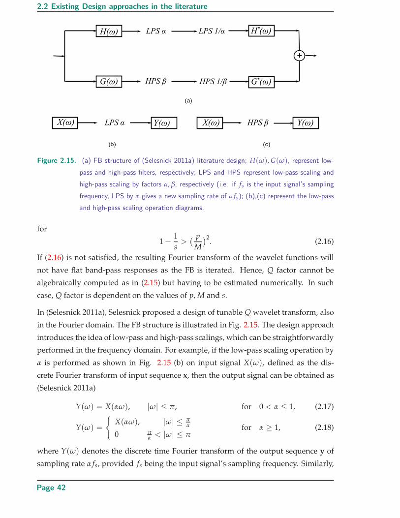
2.2 Existing Design approaches in the literature
Figure 2.15. (a) FB structure of (Selesnick 2011a) literature design; H(ω), G(ω), represent low-
pass and high-pass filters, respectively; LPS and HPS represent low-pass scaling and
high-pass scaling by factors α, β, respectively (i.e. if fs is the input signal’s sampling
frequency, LPS by α gives a new sampling rate of α fs); (b),(c) represent the low-pass
and high-pass scaling operation diagrams.
for
1 − 1
s>
( p
M
)2. (2.16)
If (2.16) is not satisfied, the resulting Fourier transform of the wavelet functions will
not have flat band-pass responses as the FB is iterated. Hence, Q factor cannot be
algebraically computed as in (2.15) but having to be estimated numerically. In such
case, Q factor is dependent on the values of p, M and s.
In (Selesnick 2011a), Selesnick proposed a design of tunable Q wavelet transform, also
in the Fourier domain. The FB structure is illustrated in Fig. 2.15. The design approach
introduces the idea of low-pass and high-pass scalings, which can be straightforwardly
performed in the frequency domain. For example, if the low-pass scaling operation by
α is performed as shown in Fig. 2.15 (b) on input signal X(ω), defined as the dis-
crete Fourier transform of input sequence x, then the output signal can be obtained as
(Selesnick 2011a)
Y(ω) = X(αω), |ω| ≤ π, for 0 < α ≤ 1, (2.17)
Y(ω) =
{
X(αω), |ω| ≤ πα
0 πα < |ω| ≤ π
for α ≥ 1, (2.18)
where Y(ω) denotes the discrete time Fourier transform of the output sequence y of
sampling rate α fs, provided fs being the input signal’s sampling frequency. Similarly,
Page 42

Chapter 2 Iterated RFB - Design challenges and literature works
if high-pass scaling is performed as in Fig. 2.15 (c), the output of such operation can be
obtained as (Selesnick 2011a)
Y(ω) =
{
X(βω + (1 − β)π), 0 < ω < π, 0 < β ≤ 1
X(βω − (1 − β)π), −π < ω < 0, 0 < β ≤ 1, (2.19)
and
Y(ω) =
0, |ω| ≤ (1 − 1β)π, β > 1
X(βω + (1 − β)π), (1 − 1β)π < ω < π, β > 1
X(βω − (1 − β)π), −π < ω < −(1 − 1β)π, β > 1
. (2.20)
Note that Y(π) = X(π) for high-pass scaling, which preserves the high-pass response
when performing high-pass scaling. Likewise, Y(0) = X(0) for low-pass scaling il-
lustrates that low-pass response should be preserved in low-pass scaling operation.
The FB structure satisfies perfect reconstruction if the low pass and high pass filters
H(ω), G(ω) satisfy
|H(ω)| = 1, for |ω| ≤ (1 − β)π, (2.21)
H(ω) = 0, for απ ≤ |ω| ≤ π, (2.22)
G(ω) = 0, for |ω| ≤ (1 − β)π, (2.23)
|G(ω)| = 1, for απ ≤ |ω| ≤ π. (2.24)
The design parameters α, β determine the filters’ frequency responses (i.e. the transi-
tion band widths) and relate to the transform redundancy and quality Q factors as
β =2
Q + 1, α = 1 − β
r(2.25)
Once the quality factor Q and redundancy factor r are specified, the corresponding de-
sign parameters α, β can be computed, hence the filters’ responses. This is an attractive
property of the design method as quality factor Q and redundancy factor r are directly
specified as opposed to the approach presented in (Bayram and Selesnick 2009a).
Table 2.1 summarises properties of the design approaches in the literature, note that
in all the approaches, the arbitrary K regularity orders can be imposed except for (Blu
1998) that K is restricted to 1.
2.3 Chapter summary
In this chapter, critical conditions for designing rational filter bank with regularity or-
ders are addressed and such FBs can be iterated to form rational DWTs. This chapter
Page 43

2.3 Chapter summary
Table 2.1. Approaches in the literature for the design of RFBs leading to RADWTs
Bi-orthogonal/ Redundant/ FIR/ PR
Orthogonal critically-sampled IIR FB
(Blu 1998) Orthogonal Critically sampled FIR FB PR
(Bayram and Orthogonal Critically sampled FIR FB near PR
Selesnick 2009b)
(Auscher 1992) Orthogonal Critically sampled IIR FB PR
(Bayram and Non-orthogonal redundant FIR FB PR
Selesnick 2009c) (tight frame)
(Bayram and Non-orthogonal redundant IIR FB PR
Selesnick 2009a) (tight frame)
(Selesnick 2011a) Tight frame redundant IIR FB PR
Proposed approach Bi-orthogonal critically-sampled FIR FB PR
provides literature review of various designs of rational DTWs and presents outlines of
their key features. The construction of rational wavelet transforms in Fourier domain
shows good advantages in attaining MRA with rational scaling factors as opposed to
the designs based on FIR FBs. However, non-compact support of the resulting wavelet
functions in time domain is a notable disadvantage, which can lead to reconstruction
errors when dealing with finite length signals. Therefore, construction of RADWTs
based on FIR filters is desirable and it is possible to to implement these in time do-
main, perhaps in real time. It should be noted that all designs in literature are based
on FIR orthogonal structure and high-pass filters are designed based on polynomial
matrix spectral factorisation. Even though this approach is reasonable in theory, the
resulting schemes can be involved when implemented. In this thesis, we propose to
design RADWTs based on a FIR bi-orthogonal structure with the inclusion of arbitrary
K regularity orders. The analysis filters are designed based on non-linear constrained
optimisation, after which the synthesis filters can be straightforwardly computed. The
rational DWT family and the corresponding filter banks will be presented in details in
the next chapters.
Page 44
Chapter 3
Bi-orthogonal RFB for FineFrequency Decomposition:
the (q−1q , 1
q) case
IN this chapter, the design of bi-orthogonal FIR rational rate filter
banks with the inclusion of K regularity orders is presented. The
FB design is formulated as a nonlinear constrained optimisation
problem. Two methods for solving this optimisation are proposed and dis-
cussed. The designs obtained from these methods are comprehensively
evaluated against the RFBs resulting from the existing approaches.
Page 45

3.1 Introduction and motivation
3.1 Introduction and motivation
The majority of wavelet designs in the literature are based on integer scaling ratios. In
the associated multi-resolution analysis, the scaling and wavelet functions between
successive levels are scaled by a given integer, with dyadic scale being by far the
most common. However, non-integer scaling ratios, equivalent to rational re-sampling
rate changes in a discretised implementation, produce sub-bands which offer better
decomposition of spectrum. This is a significant advantage for many applications
(Baussard et al. 2004, Yu and White 2005, Yu and White 2006). This chapter presents an
approach to design critically sampled two-channel FIR RFBs, with perfect reconstruc-
tion (PR), for rate change schemes satisfying ((q − 1)/q, 1/q), q > 2. Such a RFB is
depicted in Fig. 3.1. Such choice of re-sampling ratios is selected to maximise the fine
frequency decomposition property offered by rational wavelet transform over the con-
ventional dyadic case. In the literature, several designs of perfect reconstruction FIR
RFB are based on factorisation of either a para-unitary or spectral matrix (Bayram and
Selesnick 2007, Bayram and Selesnick 2009b, Bayram and Selesnick 2009c, Blu 1998),
which require the synthesis filters to be time reversed versions of the analysis filters.
The features of these designs are summarised in chapter 2. The approach presented in
this chapter discards this time reversal property to attain more degrees of freedom for
optimising the filters’ frequency selectivity. Instead, the analysis filters are designed
using non-linear constrained optimisation over the samples of their impulse response,
and the synthesis filters are then formed from products of modulated analysis filters to
ensure PR. The linear and non-linear constraints arise from regularity and PR condi-
tions, respectively. Two techniques are proposed for solving the optimisation problem
to improve the robustness against initialisations when designing K-regular PR RFBs.
This chapter is organised as follows, in section 3.2, the structure of PR RFB and re-
lated conditions such as regularity orders are discussed, followed by a formulation of
the design optimisation problem. Section 3.3 describes two approaches for solving the
optimisation problems and compares their advantages and disadvantages. Section 3.4
presents the design results and comparisons with the existing approaches and dis-
cussions. Section 3.5 discusses the RADWT shift error and the design computational
complexity. Section 3.6 contains the concluding remarks.
Page 46

Chapter 3 Bi-orthogonal RFB for Fine Frequency Decomposition: the (q−1
q , 1q ) case
Figure 3.1. Rational rate filter bank with rate changing of ( q−1q , 1
q ) (i.e p0 = 1, p1 = q − 1) (top
panel) and its equivalent uniform q-channel FB (bottom).
3.2 Design of two-channel rational filter banks
Let us start with a lemma that allows a critically sampled non-orthogonal two channel
RFB be transformed to an equivalent q-channel uniform FB.
Lemma 3.2.1. The PR rational FB in Fig. 3.2(a) design is equivalent to designing a PR q-
channel structure in Fig. 3.2(b) if and only if
HLP(z) =p0−1
∑n=0
zqnHn(zp0), FLP(z) =
p0−1
∑n=0
z−qnFn(zp0) (3.1)
HHP(z) =p1−1
∑n=0
zqnHn+p0(zp1), FHP(z) =
p1−1
∑n=0
z−qnFn+p0(zp1) (3.2)
Page 47

3.2 Design of two-channel rational filter banks
(a) two channel RFB
(b) equivalent uniform q-channel FB
Figure 3.2. Rational rate filter bank with rate changing of ( p0
q ,p1
q ) for coprime pairs (p0, q) and
(p1, q) (a) and the equivalent uniform q-channel FB (b).
Proof. We define W = e−j2π/q, Wp0 = e−j2π/p0 , Wp1= e−j2π/p1 where p0 + p1 = q. It is
straightforward to show the following holds for FB in Fig. 3.2(b)
Y(z) =1
q
[
X(z)q−1
∑n=0
Hn(z)Fn(z) + X(zW)q−1
∑n=0
Hn(zW)Fn(z) + . . . (3.3)
+ X(zWq−1)q−1
∑n=0
Hn(zWq−1)Fn(z)]
.
Consider the low-pass channel of the RFB structure in Fig. 3.2(a), let A0(z) = X(zp0)HLP(z)
which is the output of the up-sampling by p0 and followed by HLP(z) filtering, if B0(z)
denotes the output of the subsequent down-sampling by q operation it can be written
Page 48
Chapter 3 Bi-orthogonal RFB for Fine Frequency Decomposition: the (q−1
q , 1q ) case
as
B0(z) =1
q
[
A0(z1/q) + A0(z
1/qW) + . . . + A0(z1/qWq−1)
]
=1
q
[
X(zp0/q)HLP(z1/q) + X(zp0/qW p0)HLP(z
1/qW) + . . .+
+ X(zp0/qW(q−1)p0)HLP(z1/qWq−1)
]
. (3.4)
Hence, the output C0(z) of the filter by FLP(z) is
C0(z) = B0(zq)FLP(z)
=1
q
[
X(zp0)HLP(z) + X(zp0 W p0)HLP(zW) + . . .+
+ X(zp0 W(q−1)p0)HLP(zWq−1)]
FLP(z). (3.5)
Y0(z) of Fig. 3.2(a) can be written as
Y0(z) =1
p0
[
C0(z1
p0 ) + C0(z1
p0 Wp0) + . . . + C0(z1
p0 Wp0−1p0
)]
=1
qp0
[
X(z)p0−1
∑n=0
(
HLP(z1
p0 Wnp0)FLP(z
1p0 Wn
p0))
+ X(zW p0)p0−1
∑n=0
(
HLP(z1
p0 Wnp0
W)
FLP(z1
p0 Wnp0))
+ . . . + X(zW(q−1)p0)p0−1
∑n=0
(
HLP(z1
p0 Wnp0
Wq−1)FLP(z1
p0 Wnp0))]
(3.6)
Consider one component of the sum in (3.6), denoted as
Sk(z) = X(zWkp0 )p0−1
∑n=0
(
HLP(z1
p0 Wnp0
Wk)FLP(z1
p0 Wnp0))
(3.7)
Substituting (3.1), (3.2) into HLP, FLP give
Sk(z) = X(zWkp0)p0−1
∑n=0
[ p0−1
∑l=0
(
(z1
p0 Wnp0
Wk)ql Hl[(z1
p0 Wnp0
Wk)p0 ])
×
p0−1
∑m=0
(
(z1
p0 Wnp0)−qmFm[(z
1p0 Wn
p0)p0 ]
)]
= X(zWkp0)p0−1
∑n=0
[ p0−1
∑l=0
(
zqlp0 W
lnqp0
Hl(zWkp0)) p0−1
∑m=0
(
z−qm
p0 W−mnqp0
Fm(z))]
, (3.8)
since Wq = 1, Wp0p0
= 1. The product of the two sum in (3.8) will result in a sum of
products, in which each product component is
Hl(zWkp0)Fm(z)zq(l−m)
p0
p0−1
∑n=0
Wnq(l−m)p0
, (3.9)
Page 49

3.2 Design of two-channel rational filter banks
for l, m = 0, . . . p0 − 1. Note that when l 6= m, the sum ∑p0−1n=0 W
nq(l−m)p0
equals to 0.
Hence, Sk(z) is simplified to
Sk(z) = X(zWkp0)p0−1
∑n=0
Hn(zWkp0)Fn(z).
Thus Y0(z) can re-written as
Y0(z) =1
qp0
[
X(z)p0−1
∑n=0
(
Hn(z)Fn(z))
+ X(zW p0 )p0−1
∑n=0
(
Hn(zW p0)Fn(z))
+ . . .
+ X(zW(q−1)p0)p0−1
∑n=0
(
Hn(zW(q−1)p0)Fn(z))]
. (3.10)
Similarly, Y1(z) of the high-pass channel can be simplified to
Y1(z) =1
qp1
[
X(z)p1−1
∑n=0
(
Hn+p0(z)Fn+p0(z))
+ X(zW p1)p1−1
∑n=1
(
Hn+p0(zW p1)Fn+p0(z))
+ . . .
+ X(zW(q−1)p1)p1−1
∑n=0
(
Hn+p0(zW(q−1)p1)Fn+p0(z))]
. (3.11)
Combining (3.10) and (3.11) gives us Y(z) as written in (3.3)
As a result of lemma 3.2.1, and with p0 = 1, p1 = q − 1, the uniform q-channel and
2-channel rational FBs in Fig. 3.1 are equivalent if the following conditions are satisfied
H(z) =q−2
∑n=0
zqnHn(zq−1), F(z) =
q−2
∑n=0
z−qnFn(zq−1) (3.12)
3.2.1 Perfect reconstruction filter bank
The PR condition of the two channel RFB structure is constructed from the equivalent
uniform q-channel FB. The uniform q-channel FB in Fig. 3.1 satisfies PR if the synthesis
and analysis filters satisfy (Saghizadeh and Willson 1998):
Fm(z) =(−1)m det A−(0,m), (3.13)
Rm(z) =Fm(z)Hm(z), (3.14)
Page 50

Chapter 3 Bi-orthogonal RFB for Fine Frequency Decomposition: the (q−1
q , 1q ) case
such that Rm(z) is a qth-band filter4 for some m = 0, · · · , q − 1; A(z) is the alias com-
ponent (AC) matrix:
A(z) =
H0(z) H1(z) · · · Hq−1(z)
H0(zW) H1(zW) · · · Hq−1(zW)...
......
...
H0(zWq−1) H1(zWq−1) · · · Hq−1(zWq−1)
, (3.15)
where W = ej2π/q and A−(0,m) denotes matrix A with row 0 and column m deleted.
Such choice of analysis/synthesis relationship (3.13) guarantees the FB structure is
alias free and synthesis filters are real coefficient FIR if the analysis filters are real FIR
filters. If h and hq−1 are the column vectors representing the impulse responses of the
analysis low- and high-pass filters of the RFB structure in Fig. 3.1, respectively and rm
represents the impulse response of the filter Rm(z) of equation (3.14), the PR condition
can be formulated as
rm,k(h, hq−1) ≡[
0tk0−1 α 0t
B−k0
]t, (3.16)
where rm,k denotes the k-th q-polyphase component of the impulse response rm of
Rm(z), 0l is a zero vector of length l; B and k0 are positive integers. In other words,
one of the q polyphase components of rm is required to equal to a pure delay. Note that
the condition in (3.16) is only required to satisfy one integer index value m ∈ [0, q − 1]
as satisfying for one results in satisfying for all others due to the relationship in (3.13).
From (3.13), (3.14) we can write Rm(z) as (−1)m det A−(0,m)Hm(z), where A is a q ×q matrix of Hm(zWk) entries (k = 0, . . . , q − 1). Hence, if we consider the impulse
response of Hm(z) as unknowns, the impulse response of Rm(z) will be a function of
Hm(z)’s for m = 0, . . . , q − 1 with the unknowns’ highest order being q.
3.2.2 Vanishing moments and regularity orders
A rational wavelet transform is defined to have K vanishing moments if the corre-
sponding RFB satisfies: 1) the analysis high-pass filter possesses a factor of (1 − z−1)K,
and 2) the analysis and synthesis low-pass filters are divisible by (1 + z−1 + · · · +z−(q−2))K and (1+ z−1 + · · ·+ z−(q−1))K, respectively (Bayram and Selesnick 2009c). It
is customary to normalise the analysis low-pass filter’s response to be√
q − 1 at ω = 0
4qth-band filter is defined as filters with pass-band response in the region of [ k0πq , k1π
q ] for intergers
k0, k1; k0 < k1 ≤ q and one of its q-polyphase is a pure delay
Page 51
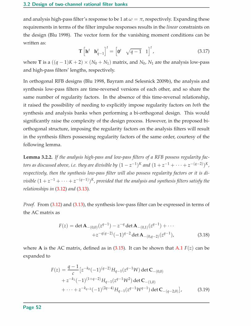
3.2 Design of two-channel rational filter banks
and analysis high-pass filter’s response to be 1 at ω = π, respectively. Expanding these
requirements in terms of the filter impulse responses results in the linear constraints on
the design (Blu 1998). The vector form for the vanishing moment conditions can be
written as:
T[
ht htq−1
]t=
[
0t√
q − 1 1]t
, (3.17)
where T is a ((q − 1)K + 2)× (N0 + N1) matrix, and N0, N1 are the analysis low-pass
and high-pass filters’ lengths, respectively.
In orthogonal RFB designs (Blu 1998, Bayram and Selesnick 2009b), the analysis and
synthesis low-pass filters are time-reversed versions of each other, and so share the
same number of regularity factors. In the absence of this time-reversal relationship,
it raised the possibility of needing to explicitly impose regularity factors on both the
synthesis and analysis banks when performing a bi-orthogonal design. This would
significantly raise the complexity of the design process. However, in the proposed bi-
orthogonal structure, imposing the regularity factors on the analysis filters will result
in the synthesis filters possessing regularity factors of the same order, courtesy of the
following lemma.
Lemma 3.2.2. If the analysis high-pass and low-pass filters of a RFB possess regularity fac-
tors as discussed above, i.e. they are divisible by (1 − z−1)K and (1 + z−1 + · · ·+ z−(q−2))K,
respectively, then the synthesis low-pass filter will also possess regularity factors or it is di-
visible (1 + z−1 + · · ·+ z−(q−1))K, provided that the analysis and synthesis filters satisfy the
relationships in (3.12) and (3.13).
Proof. From (3.12) and (3.13), the synthesis low-pass filter can be expressed in terms of
the AC matrix as
F(z) = det A−(0,0)(zq−1)− z−q det A−(0,1)(z
q−1) + · · ·+z−q(q−2)(−1)q−2 det A−(0,q−2)(z
q−1), (3.18)
where A is the AC matrix, defined as in (3.15). It can be shown that A.1 F(z) can be
expanded to
F(z) =q − 1
c
[z−k0(−1)(q−2)Hq−1(z
q−1W)det C−(0,0)
+ z−k1(−1)(1+q−2)Hq−1(zq−1W2)det C−(1,0)
+ · · ·+ z−kq−2(−1)(2q−4)Hq−1(zq−1Wq−1)det C−(q−2,0)
], (3.19)
Page 52

Chapter 3 Bi-orthogonal RFB for Fine Frequency Decomposition: the (q−1
q , 1q ) case
where
C =
H(zWq−1) H(zWq−1Wp) · · · H(zWq−1Wq−2p )
H(zWq−2) H(zWq−2Wq−2p ) · · · H(zWq−2Wp)
......
......
H(zW) H(zWWp) · · · H(zWWq−2p )
(3.20)
and W = ej2π/q, Wp = ej2π/(q−1), c is a constant, k0, · · · , kq−2 ∈ Z . (3.19) can be
verified by substituting a specific value of q ≥ 3 and expanding the corresponding
determinant of C. For example, for q = 3, (3.19) holds for k0 = k1 = 3, c = −2. Since
H(z) is divisible by (zq−2 + · · · + z + 1)K and Hq−1(z) is divisible by (z − 1)K, there
exists T0(z) and T1(z) such that
H(z) =[(z − Wp) . . . (z − W(q−2)p )]KT1(z), (3.21)
Hq−1(z) =(z − 1)KT0(z). (3.22)
We need to show that if (3.19)–(3.22) are satisfied, then F(z) will be divisible by (1 +
z + · · ·+ zq−1)K. Consider the first term of the sum in (3.19), define
P1(z) = Hq−1(zq−1W)det C−(0,0) = (zq−1W − 1)KT0(z
q−1W)det C−(0,0). (3.23)
Therefore, P1(z) will have K zeros at zq−1 = W−1 = e−j2π/q or equivalently, at frequen-
cies ωn0 =−2π
q(q−1)+ 2πn0
(q−1)for n0 = 1, · · · , q − 1. From (3.20):
det C−(0,0) = det
H(zWq−2Wp) · · · H(zWq−2Wq−2p )
......
...
H(zWWp) · · · H(zWWq−2p )
=∑m
(−1)mq−2
∏n1,n2=1
H(zWn1Wn2p )
︸ ︷︷ ︸
Nm
, (3.24)
where any Nm is a product term which contains terms of the form H(zW lWn2p )H(zWn1W l
p)
for arbitrary integers 1 ≤ l, n1, n2 ≤ q − 2. Substitute (3.21) into (3.24):
det C−(0,0) =∑m
(−1)mq−2
∏n1,n2=1
[
(zWn1Wn2p − Wp) . . . (zWn1Wn2
p − W(q−2)p )
]KT1(zWn1Wn2
p )
=∑m
(−1)m{ q−2
∏n1,n2,n3=1
(zWn1Wn2p − Wn3
p )KT1(zWn1Wn2p )
}
. (3.25)
Therefore, each product term Nm of det C−(0,0) will have zeros at ωn1n2n3 = 2πn3(q−1)
−[
2πn1q + 2πn2
(q−1)
]
; n1, n2, n3 = 1, · · · , q − 2 and p = q − 1. As a consequence, it is
Page 53

3.2 Design of two-channel rational filter banks
always possible to find common zeros at frequencies ωn1n2n3 = − 2πn1q by choosing
n1 ∈ [1, q − 2] and n3 = n2. In other words, det C−(0,0) will have K-multiple zeros at
ω = − 2πq , · · · ,− 2(q−2)π
q , or equivalently, at l2πq , 2 ≤ l ≤ q − 2. Including the common
zeros at 2π/q from high-pass filter Hq−1(zq−1W) discussed earlier, P1(z) will therefore
have K-multiple zeros at frequencies l2πq , 1 ≤ l ≤ q − 2. By similar arguments, it is
straight forward to show that other product terms of F(z) will have zeros at the above
frequencies. It follows that the synthesis low-pass filter has K regularity factors.
This result allows us to design a bi-orthogonal RFB by designing the analysis side with
K regularity factors independently. The synthesis side is then fully determined from
(3.12)–(3.13) and will automatically have K regularity factors as well. This forms the
strategy underlying the design approach presented in this chapter.
3.2.3 Least square optimisation
The issue of shift-variance of rational DWTs has been discussed in literature (Blu 1993,
Blu 1998, Bayram and Selesnick 2009c) and this is summarised in chapter 2. This prop-
erty prevents the iterated RFB to behave like a rational DWT, as the iterated RFB will
not converge to a unique wavelet function. An illustration of the shift-variance issue is
shown in Fig. 2.7 of chapter 2.
To suppress this effect, it has been shown (Blu 1993, Blu 1998, Bayram and Selesnick
2009c) that good frequency selectivity in the RFB filters reduces the shift error, defined
as the maximum of absolute error between the (q − 1)i discrete time sequences being
shifted on the same interval (Blu 1993). Our proposed design approach therefore seeks
to achieve good frequency selectivity by using least squares optimisation, with the
objective function being defined as:
f = α0
∫ π
ωsLP
|H(ω)|2 dω + α1
∫ ωsHP
0|Hq−1(ω)|2 dω, (3.26)
where ωsLP = πq +∆ωLP, ωsHP =
(q−1)πq −∆ωHP are the stop-band edge frequencies of
the analysis low-pass and high-pass filters, respectively, and α0, α1 ≥ 0 are adjustable
weights. In vector form, the objective function can be written as:
f (h, hq−1) = α0htMLPh + α1htq−1MHPhq−1, (3.27)
Page 54

Chapter 3 Bi-orthogonal RFB for Fine Frequency Decomposition: the (q−1
q , 1q ) case
where MLP and MHP are positive semi-definite matrices whose entries depend solely
on design parameters ωsLP and ωsHP, respectively. The matrices are defined as
[
MLP
]
i,j=
− 2 sin((i−j)ωsLP)π(i−j)
i 6= j
2(1 − ωsLP
π
)i = j
, (3.28)
[
MHP
]
i,j=
2 sin((i−j)ωsHP)π(i−j)
i 6= j
2ωsHPπ i = j
. (3.29)
The RFB design problem, which we label as (P), can be formulated as an optimisation
problem that minimises f (h, hq−1) in (3.27), subject to the conditions in (3.16)–(3.17).
3.3 Solving the design problem
The optimisation problem (P) is non-convex since the PR constraints (3.16) have high-
est order q ≥ 3 and hence are non-convex. Nonlinear optimisation is the term used
to describe problems whose objective or constraint functions are nonlinear where the
convexity is not guaranteed. For such problems, effective methods to find the global
solution are also not guaranteed.
In this chapter, we propose two approaches to solve problem (P): local optimisation
and linearisation. The first approach, local optimisation approach abandons finding
the global solution of the problem in favor of finding ‘good enough’ local solution
based on an appropriate initialisation to the problem. In the latter, a compromise is
made by fixing some variables of the multivariate problem to reduce the order of the
non-linear constraints to one, thus leading to a two stage method of solution.
3.3.1 Local optimisation of the non-linear problem
The local optimisation approach proceeds in two stages. An approximate optimum is
first found by solving a simplified sub-problem, which is then used to initialise a line-
search algorithm to find a solution to the original problem 5. This proposed approach
aims to improve the robustness against initialisation of the optimisation problem (P)
by first solving a convex sub-problem (P0), this sub-problem is obtained by removing
5fmincon and the active-set (line search) sub-algorithm of Matlab is used as the optimisation algo-
rithm
Page 55

3.3 Solving the design problem
the PR constraint (3.16) from (P). Instead, convex constraints (3.30) are introduced to
ensure the global solution found by (P0) satisfy the PR condition approximately.
The proposed RFB satisfies PR if Rm(z) described in (3.14) is a qth-band filter, or equiv-
alently, one of its q-polyphase components is a pure delay (see (3.16)). Therefore, if we
choose m = q − 1, Rq−1(z) is required to be approximately qth-band as a result of (P0)
with pass-band response in the region of [q−1
q π, π]. This can be achieved by individ-
ually requiring the respective q-polyphase components of h and hq−1 to approximate
pure delays, within some set tolerance bounds in the coefficient values. Such bounding
constraints are convex:
|h(m0)| ≤ εLP,∣∣hq−1(m1)
∣∣ ≤ εHP, (3.30)
Hence, (P0) can be formulated as
Problem (P0)
minh,hq−1
f (h, hq−1) as defined in (3.27), subject to (3.17), and
|h(m0)| ≤ εLP,∣∣hq−1(m1)
∣∣ ≤ εHP
for
m0 = L0 ± kq, 0 ≤ m0 ≤ N0, L0 = bN0/2c ± c0
m1 = L1 ± kq, 0 ≤ m1 ≤ N1, L1 = bN1/2c ± c1
,
where L0, L1 are non-zero integers and εLP, εHP are small positive real valued param-
eters; N0, N1 denotes the low-pass h and high-pass hq−1 filters’ lengths, respectively;
k, c0, c1 ∈ N, k 6= 0. Optimising f (h, hq−1) in (3.27) subject to such polyphase bound
constraints lead to global solutions of (P0) such that H(z), Hq−1(z) have nearly flat
pass-bands in [0, πq ], [
(q−1)πq , π], respectively. The relationship between polyphase com-
ponent flatness and filters’ pass-band flatness is discussed in appendix A.2.
Claim 3.3.1. Consider H(z) to be a low-pass filter of the FB structure in Fig. 3.1 having
flat pass-bands in [0, πq ], if the resulting synthesis filter Fq−1(z) filter is defined by (3.13) as
Fq−1(z) = (−1)q−1 det A−(0,q−1)(z), then Fq−1(z) is a high-pass filter with flat pass-band
response in [ (q−1)πq , π].
Page 56

Chapter 3 Bi-orthogonal RFB for Fine Frequency Decomposition: the (q−1
q , 1q ) case
Proof. The low-pass filter H(z) having flat pass-band in [0, πq ] results in its q− 1 polyphase
components H0, · · · , Hq−2 having flat pass-band in [0,(q−1)π
q ]; Fq−1(z) = (−1)m×det A−(0,q−1)(z) where A(z) is defined in (3.15) suggests that Fq−1(z) is dependent on
the modulated polyphases H0(zWn0), · · · , Hq−2(zWnq−2), n0, · · · , nq−2 = 1, · · · , q − 1.
If we apply Laplace expansion on det A−(0,q−1)(z), we attain a sum of (q − 1)! product
components, each of which can be defined as:
pk(z) =[H0(zWn0)× . . . × Hq−2(zWnq−2)
](3.31)
for any index k = 1, · · · , (q − 1)! corresponding to a choice of the combination of
n0, · · · , nq−2 = 1, . . . , q − 1 such that n0 6= n1 6= · · · 6= nq−2. In the following we
show that each of the product term in (3.31) has its magnitude |pk(ω)| being flat in
its pass-band response in [ (q−1)πq , π] as a result of the assumption that H0, . . . , Hq−2 all
have flat pass-band response in [0,(q−1)π
q ]. Let |Hi(z)|, i = 0, · · · , q − 2 and |Hi(zW)|have frequency response as shown in Fig. 3.3. By induction, we can verify that for any
|Hi(zWn)|, n = 1, · · · , q − 1, the corresponding stop-band region varies across all fre-
quencies except for ω ∈ [ q−1q π,
q+1q π]. Hence the product filter |pk(ω)| is a high-pass
filter with flat pass-band response in the frequency region of ω ∈ [q−1
q π,q+1
q π].
The phase response in the pass-band region of the product term pk(ω) is the sum of
all the phases of H0, . . . , Hq−2 in their pass-band regions. Thus the filter’s phase is ap-
proximately constant as k varies. This results in Fq−1(z) having flat pass-band response
in [q−1
q π,q+1
q π] or ±[q−1
q π, π] as Fq−1(z) is a real coefficient FIR filter.
As a result, the synthesis high-pass response is greatly dependent on the analysis low-
pass response. Even though the proof is shown for ideal brick wall filter, its use is only
to illustrate the approach and the property also applies for non-ideal filters. Thus, if the
analysis low-pass filter H(z) is a real non-ideal filter with good stop band, transition
band and nearly flat pass-band responses, then similar property can be attained for the
resultant synthesis high-pass filter Fq−1(z). Hence, the global solution of problem (P0)
results in the high-pass filters Hq−1(z), Fq−1(z) with good flatness in their pass-band.
Also, since two of their q-polyphase components are approximate delays as a result of
(3.30), the product filter Rq−1(z) = Hq−1(z)Fq−1(z) has a good flatness in its pass-band
region, that is, approximates a qth-band filter with pass-band response in [(q−1)π
q , π].
The design of qth-band filters based on least square criterion and subject to linear con-
straints has been studied in (Wisutmethangoon and Nguyen 1999). The filters obtained
Page 57
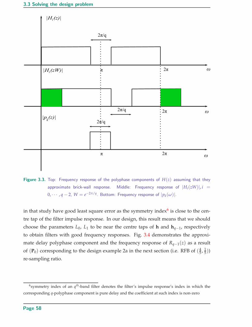
3.3 Solving the design problem
Figure 3.3. Top: Frequency response of the polyphase components of H(z) assuming that they
approximate brick-wall response. Middle: Frequency response of |Hi(zW)|, i =
0, · · · , q − 2, W = e−2π/q. Bottom: Frequency response of |pk(ω)|.
in that study have good least square error as the symmetry index6 is close to the cen-
tre tap of the filter impulse response. In our design, this result means that we should
choose the parameters L0, L1 to be near the centre taps of h and hq−1, respectively
to obtain filters with good frequency responses. Fig. 3.4 demonstrates the approxi-
mate delay polyphase component and the frequency response of Rq−1(z) as a result
of (P0) corresponding to the design example 2a in the next section (i.e. RFB of (45 , 1
5))
re-sampling ratio.
6symmetry index of an qth-band filter denotes the filter’s impulse response’s index in which the
corresponding q-polyphase component is pure delay and the coefficient at such index is non-zero
Page 58
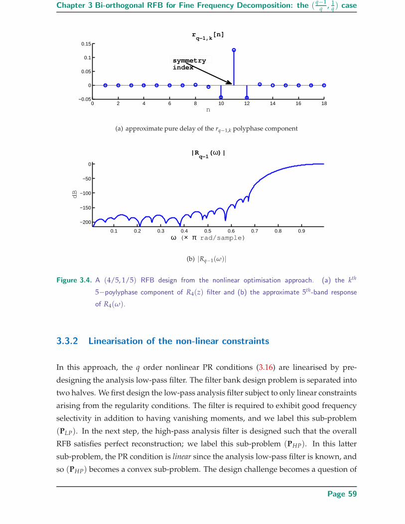
Chapter 3 Bi-orthogonal RFB for Fine Frequency Decomposition: the (q−1
q , 1q ) case
0 2 4 6 8 10 12 14 16 18−0.05
0
0.05
0.1
0.15
n
rq−1,k
[n]
symmetryindex
(a) approximate pure delay of the rq−1,k polyphase component
0.1 0.2 0.3 0.4 0.5 0.6 0.7 0.8 0.9
−200
−150
−100
−50
0
ω ( × π rad/sample)
dB
|Rq−1
( ω)|
(b) |Rq−1(ω)|
Figure 3.4. A (4/5, 1/5) RFB design from the nonlinear optimisation approach. (a) the kth
5−poylyphase component of R4(z) filter and (b) the approximate 5th-band response
of R4(ω).
3.3.2 Linearisation of the non-linear constraints
In this approach, the q order nonlinear PR conditions (3.16) are linearised by pre-
designing the analysis low-pass filter. The filter bank design problem is separated into
two halves. We first design the low-pass analysis filter subject to only linear constraints
arising from the regularity conditions. The filter is required to exhibit good frequency
selectivity in addition to having vanishing moments, and we label this sub-problem
(PLP). In the next step, the high-pass analysis filter is designed such that the overall
RFB satisfies perfect reconstruction; we label this sub-problem (PHP). In this latter
sub-problem, the PR condition is linear since the analysis low-pass filter is known, and
so (PHP) becomes a convex sub-problem. The design challenge becomes a question of
Page 59

3.4 Filter design results
how to design H(z) such that Hq−1(z) has the shortest possible length while satisfying
all desired properties.
The design problem is decomposed into two sub-problems as follows:
Problem (PLP): Designing low-pass filter by minimisation
minh
f (h) = htMLPh, subject to
TLPh =[
0t√
q − 1]t
, (3.32)
|h(m0)| ≤ εLP, (3.33)
where MLP is the positive semi-definite matrix described in Section 3.2.3, TLP is con-
structed based on regularity conditions imposed on the analysis low-pass filter as
in (3.17). When H(z) is known, then so is Fq−1(z). The product Rq−1(z) = Fq−1(z)Hq−1(z)
can be written in matrix form as rq−1 = Fh; where rq−1 is a column vector representing
the impulse response of the filter Rq−1(z), F is a N f × N1 Toeplitz matrix containing
the coefficients of the filter Fq−1 and N f is the filter’s length.
Problem (PHP): Designing a matching PR high pass filter by minimisation
minhq−1
f (hq−1) = htq−1MHPhq−1, subject to
THPhq−1 =[
0t 1]t
,
rq−1(hq−1) = Fq−1hq−1 ≡[
0t α 0t]t
, (3.34)
where Fq−1 is aN f
q × N1 matrix obtained by choosing rows corresponding to zero co-
efficient index from matrix F, N1 is the length of the vector hq−1; THP is the regularity
matrix derived from (3.17). We choose m0 = L0 ± kq of subproblem (PLP) such that L0
approximates N0/2 since it is desirable for the overall system delay n0 to be close to
the mid-point index of rq−1.
Fixing the analysis low-pass filter simplifies the PR constraints order to one and at the
same time significantly reduces the variables of the optimisation. The advantage of this
method is that our PR conditions are always kept linear regardless of the rate changing
parameter q, which is most useful for large q.
Page 60

Chapter 3 Bi-orthogonal RFB for Fine Frequency Decomposition: the (q−1
q , 1q ) case
Table 3.1. The filter design parameters
(a) Local optimisation parameters
Local optimisation method
Example 1a: Example 1b: Example 2a: Example 2b:
(2/3, 1/3), (2/3, 1/3), (4/5, 1/5), (4/5, 1/5),
K = 1 K = 3 K = 1 K = 3
n0, L0, N0 31, 18, 35 31, 20, 38 46, 26, 50 51, 28, 50
L1, N1 10, 20 10, 20 14, 28 18, 35
ωsLPπ3 + 0.07π π
3 + 0.07π π5 + 0.07π π
5 + 0.07π
ωsHP2π3 − 0.1π 2π
3 − 0.1π 4π5 − 0.1π 4π
5 − 0.1π
(b) Linearised parameters
Linearised method
Example 3a: Example 3b: Example 4a: Example 4b: Example 5:
(2/3, 1/3), (2/3, 1/3), (4/5, 1/5), (4/5, 1/5), (5/6, 1/6),
K = 1 K = 3 K = 1 K = 3 K = 3
n0, L0, N0 31, 16, 30 31, 16, 30 46, 20, 38 51, 22, 42 64, 33, 65
N1 28 28 40 43 35
ωsLPπ3 + 0.07π π
3 + 0.07π π5 + 0.06π π
5 + 0.06π π6 + 0.032π
ωsHP2π3 − 0.11π 2π
3 − 0.11π 4π5 − 0.11π 4π
5 − 0.1π 5π6 − 0.08π
3.4 Filter design results
In this section, four design examples based on local optimisation and five examples
based on the linearised approach are presented. The designs’ parameters are sum-
marised in Table 3.1 (a), (b). The obtained RFB all satisfy PR with reconstruction error
in the order of 10−10. Most of the frequency response comparisons are made with re-
spect to the designs described in (Blu 1998) since that is the only reported FIR critically
sampled structure which satisfies PR condition and possesses one regularity order.
Note that for Blu’s approach, higher regularity orders cannot be attained. In (Bayram
and Selesnick 2009b)’s approach, it is capable of producing arbitrary number of reg-
ularity orders, but the RFB design does not satisfy PR condition. Instead only near
PR is obtained in such design. To complete the comparison, we also compare against
Bayram and Selesnick’s design in one example. The filters’ lengths are shown in table
3.2.
Page 61

3.4 Filter design results
0 0.2 0.4 0.6 0.8 1−100
−80
−60
−40
−20
0
Synthesis low pass filters
ω (×π rad/sample)0 0.2 0.4 0.6 0.8 1
−100
−80
−60
−40
−20
0
Analysis low pass filters
ω (×π rad/sample)
0 0.2 0.4 0.6 0.8 1−100
−80
−60
−40
−20
0
Synthesis highpass filters
ω (×π rad/sample)
dB
0 0.2 0.4 0.6 0.8 1−100
−80
−60
−40
−20
0
Analysis highpass filters
ω (×π rad/sample)
linearised approach − 1 regularity oderlocal optimisation − 1 regularity oder(Blu 1998) − 1 regularity order
(a) (2/3, 1/3) RFB filters’ responses - one regularity order
0 0.2 0.4 0.6 0.8 1−100
−80
−60
−40
−20
0
Synthesis low pass filters
ω (×π rad/sample)
dB
0 0.2 0.4 0.6 0.8 1−100
−80
−60
−40
−20
0
Analysis low pass filters
ω (×π rad/sample)
0 0.2 0.4 0.6 0.8 1−100
−80
−60
−40
−20
0
Synthesis highpass filters
ω (×π rad/sample)0 0.2 0.4 0.6 0.8 1
−100
−80
−60
−40
−20
0
Analysis highpass filters
ω (×π rad/sample)
linearised approach − 1 regularity oderlocal optimisation − 1 regularity oder(Blu 1998) − 1 regularity order
(b) (4/5, 1/5) RFB filters’ responses - one regularity order
Figure 3.5. Comparisons between the proposed approaches of RFBs (2/3, 1/3) (a), (4/5, 1/5)
(b) with one regularity order versus literature (Blu 1998) of the same re-sampling rates
and regularity order. From left to right: Top panels show the low-pass synthesis and
analysis filters’ frequency responses, respectively; bottom panels show the high-pass
synthesis and analysis filters’ frequency responses, respectively. Red solid and dashed
traces represent linearised and local optimisation designs, respectively while blue dash
illustrates literature (Blu 1998) design.
Page 62

Chapter 3 Bi-orthogonal RFB for Fine Frequency Decomposition: the (q−1
q , 1q ) case
Fig. 3.5 illustrates the filters’ frequency responses of example 1a, 3a (a) and example 2a,
4a (b) comparing to (Blu 1998) of the same re-sampling rates and regularity order, re-
spectively. The filters’ lengths are selected such that for each design, the total number
of taps are approximately equal between the design methods. It can be seen that for
one regularity order, both proposed methods result in wider transition band width as
compared to the literature (Blu 1998). However, it should be noted that (Blu 1998) does
not lead to RFB with high regularity while the proposed bi-orthogonal structure does.
With the orthogonality property relaxed for our designs, we are free to impose higher
regularity order than the design in (Blu 1998), which has the effect of increasing the
smoothness of the scaling functions (Bayram and Selesnick 2007). This underlines the
greatest improvement as compared to the existing literature (Blu 1998). In Fig. 3.6
frequency responses of RFB with three regularity orders designed based on the two
proposed methods are plotted against each other. In Fig. 3.6 (a), both the proposed
methods illustrate similar filters’ frequency responses for re-sampling rates (2/3, 1/3)
design. In Fig. 3.6 (b), the local optimisation method results in better frequency re-
sponses in analysis low-pass and synthesis high-pass filters while it is inferior in the
analysis high-pass response. It should be noted that linearised method is better used
in cases of high value parameter q since such parameter corresponds to the highest or-
der of the non-linear constraints in the local optimisation method, which significantly
increase the design complexity. For example the (5/6, 1/6) RFB with three regularity
orders in example 5, is designed using the linearised approach. The designed filters
are plotted against (Blu 1998) in Fig. 3.7 (a), (b). In Fig. 3.8 the father wavelet func-
tions are illustrated. In appendix B.1.3, B.1.4, filter designs based on linearised method
of higher q parameters are shown (for q = 7, 10). Note that only linearised method
should be used for such high values of q since the complexity of solving high order
nonlinear constraints of the local optimisation method increases significantly in those
cases, which can lead to impractically long running time. To complete the comparison,
filters’ frequency responses of the RFB (4/5, 1/5) structure with three regularity orders
are plotted against the literature (Bayram and Selesnick 2009b) of the same regularity
orders and shown in Fig. 3.7 (c), (d). In the comparison with Bayram’s design (Bayram
and Selesnick 2009b), the transition band and stop band performance have improved
with the same number of regularity orders imposed. This is illustrated in Fig. 3.7 (c),
(d). Most importantly, our proposed design results in PR FBs, where reconstruction
error is in the order of 10−10, with arbitrary K orders of regularity while the literature
Page 63

3.4 Filter design results
0 0.2 0.4 0.6 0.8 1−100
−50
0
Synthesis low pass filters
ω ( ×π rad/sample)0 0.2 0.4 0.6 0.8 1
−100
−50
0
Analysis low pass filters
ω ( ×π rad/sample)
0 0.2 0.4 0.6 0.8 1−100
−50
0
Synthesis highpass filters
ω ( ×π rad/sample)
dB
0 0.2 0.4 0.6 0.8 1−100
−50
0
Analysis highpass filters
ω ( ×π rad/sample)
local optimisation − 3 regularity oders linearised approach − 3 regularity oders
(a) (2/3, 1/3) RFB filters’ responses - three regularity orders
0 0.2 0.4 0.6 0.8 1−100
−50
0
Synthesis low pass filters
ω (×π rad/sample)0 0.2 0.4 0.6 0.8 1
−100
−50
0
Analysis low pass filters
ω (×π rad/sample)
0 0.2 0.4 0.6 0.8 1−100
−50
0
Synthesis highpass filters
ω (×π rad/sample)
dB
0 0.2 0.4 0.6 0.8 1−100
−50
0
Analysis highpass filters
ω (×π rad/sample)
local optimisation − 3 regularity oders linearised approach − 3 regularity oders
(b) (4/5, 1/5) RFB filters’ responses - three regularity orders
Figure 3.6. Comparison between proposed methods for (2/3, 1/3) (a) and (4/5, 1/5) (b) RFBs
with three regularity orders. From left to right: Top panels show the low-pass synthesis
and analysis filters’ frequency responses, respectively; bottom panels show the high-
pass synthesis and analysis filters’ frequency responses, respectively. Red solid traces
represents local optimisation filters while dashed blue represents linearised filters.
counterpart (Bayram and Selesnick 2009b) only attains near PR FBs (reconstruction er-
ror is approximately 10−4).
Page 64
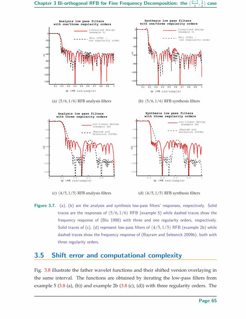
Chapter 3 Bi-orthogonal RFB for Fine Frequency Decomposition: the (q−1
q , 1q ) case
0.1 0.2 0.3 0.4 0.5 0.6 0.7 0.8 0.9 1
−140
−120
−100
−80
−60
−40
−20
0
Analysis low pass filters with one/three regularity orders
dB
ω ( ×π rad/sample)
linearized design(example 5)
(Blu 1998) −one regularity order
(a) (5/6, 1/6) RFB analysis filters
0.1 0.2 0.3 0.4 0.5 0.6 0.7 0.8 0.9 1
−120
−100
−80
−60
−40
−20
0
Synthesis low pass filters with one/three regularity orders
ω ( ×π rad/sample)
dB
linearised design(example 5)
(Blu 1998) − one regularity order
(b) (5/6, 1/6) RFB synthesis filters
0 0.2 0.4 0.6 0.8 1
−120
−100
−80
−60
−40
−20
0
Analysis low pass filters with three regularity orders
ω ( ×π rad/sample)
dB
non−linear design(example 2b)
(Bayram andSelesnick 2009b)
(c) (4/5, 1/5) RFB analysis filters
0.2 0.4 0.6 0.8 1
−120
−100
−80
−60
−40
−20
0
Synthesis low pass filters with three regularity orders
ω ( ×π rad/sample)
dB
non−linear design (example 2b)
(Bayram andSelesnick 2009b)
(d) (4/5, 1/5) RFB synthesis filters
Figure 3.7. (a), (b) are the analysis and synthesis low-pass filters’ responses, respectively. Solid
traces are the responses of (5/6, 1/6) RFB (example 5) while dashed traces show the
frequency response of (Blu 1998) with three and one regularity orders, respectively.
Solid traces of (c), (d) represent low-pass filters of (4/5, 1/5) RFB (example 2b) while
dashed traces show the frequency response of (Bayram and Selesnick 2009b), both with
three regularity orders.
3.5 Shift error and computational complexity
Fig. 3.8 illustrate the father wavelet functions and their shifted version overlaying in
the same interval. The functions are obtained by iterating the low-pass filters from
example 5 (3.8 (a), (b)) and example 2b (3.8 (c), (d)) with three regularity orders. The
Page 65

3.5 Shift error and computational complexity
28 29 30 31 32 33 34 35 36
−0.1
0
0.1
0.2
0.3
0.4
0.5
Analysis father wavelet
fatherwavelet function
shiftedtranslated version
(a) Linearised design (5/6, 1/6) RFB analy-
sis father wavelet
162 164 166 168 170 172 174 176 178
−0.1
0
0.1
0.2
0.3
0.4
0.5
Synthesis father wavelet
father wavelet function
shifted translated version
(b) Linearised design (5/6, 1/6) RFB synthe-
sis father wavelet
50 52 54 56 58 60 62 64 66 68 70
−0.1
0
0.1
0.2
0.3
0.4
0.5
Analysis father wavelet
fatherwavelet function
shiftedtranslated version
(c) Local optimisation design (4/5, 1/5) RFB
analysis father wavelet
122 124 126 128 130 132 134 136 138
−0.1
0
0.1
0.2
0.3
0.4
0.5
Synthesis father wavelet
fatherwavelet function
shiftedtranslated version
(d) Local optimisation design (4/5, 1/5)RFB
synthesis father wavelet
Figure 3.8. Father wavelet functions of example 5 (a), (b) and example 2b (c), (d). Red traces
of (a), (b) are the analysis/synthesis father wavelet functions obtained from iterating
the low-pass filters of example 5 ((5/6, 1/6) RFB) and (c), (d) are the functions of
example 2b ((4/5, 1/5) RFB), both with three regularity orders. The blue traces in all
plots represent the translated version of he functions being shifted to the same interval.
maximum shift error, defined as maximum error between any two limit functions be-
ing shifted on the same interval (Blu 1993), is used to measure the shift variance of
our designs. With scaling functions obtained from iterating the synthesis and analysis
scaling filters 25 times, the maximum shift errors are measured to be approximately
0.02 and 0.008 for example 2b and 5, respectively.
To demonstrate the difference of computations between the cases of (5/6, 1/6), if we
consider the multiply-add operation as a measure for computation, for the filters’
length as illustrated in Table 3.1(b) the total number of multiply-add operations in our
Page 66
Chapter 3 Bi-orthogonal RFB for Fine Frequency Decomposition: the (q−1
q , 1q ) case
design is approximately 75Lx, compared to Blu’s design of 78Lx, where Lx is the input
signal’s length. It should be noted that as different to orthogonal method in (Blu 1998),
in which the analysis filters have the same lengths as the synthesis filters, the pro-
posed methods are bi-orthogonal and the synthesis low-pass filters are determined by
(q − 2)N0 + (q − 1)N1 − A. The parameters N0, N1 represent the analysis low-pass and
high-pass filters’ lengths, respectively; q determines the re-sampling ratio of the RFB
structure and A is a constant which varies with re-sampling ratio parameter q. This
results in lengthy synthesis low-pass filter compared with the analysis filters. In the
proposed RFB design, PR conditions are imposed by forcing Rq−1(z) filter to be a qth-
band filter. The number of PR conditions will always be approximately N0+N1q , where
N0 + N1 represents the total number of variables of the optimisation. It differs from
the orthogonal case in which the number of orthogonal conditions is in the order of
N/2 + C, where C is some constant depending on rate changing parameters p, q and
N is a total number of variables. For example, in Blu’s (5/6, 1/6) design (Blu 1998),
there are 168 conditions for 199 unknowns, while in our example 5, N0 = 65, N1 = 35
leads to 15 PR conditions for 100 unknowns. The proposed design approach in this
thesis thus provides greater degrees of freedom (fewer constraints) in filter design de-
spite having to deal with high order (q) polynomials as PR conditions. In orthogonal
FBs, the orthogonal conditions are always quadratic regardless of the values of p and
q.
3.6 Chapter summary
In this chapter, we have presented a method of designing a (q − 1/q, 1/q) rational
filter bank with general K regularity orders together with two approaches to solve the
nonlinear optimisation problem which improves the robustness against initialisations.
The filters’ frequency selectivity are optimised to enable the designs to approximate
rational DWTs. The design method is potentially useful for filter bank designs with
more general (p/q, (q − p)/q) since the relationship between the regularity factors of
analysis and synthesis filters is valid for more general cases of q − p > 1. However,
for such regimes, the linearized method described here cannot be used. In the next
chapter, we address the design of more general p, q pairs, which lead to more flexible
Q factor rational DWTs.
Page 67

3.6 Chapter summary
Table 3.2. Filters’ lengths comparison
Analysis Synthesis Analysis Synthesis Regularity
low-pass low-pass high-pass high-pass K
Local optimisation approach
Example 1a (23 , 1
3) 35 76 20 34 K = 1
Example 1b (23 , 1
3) 38 75 280 37 K = 3
Example 2a (45 , 1
5) 50 212 28 44 K = 1
Example 2b (45 , 1
5) 50 244 35 45 K = 3
Linearised approach
Example 3a (23 , 1
3) 30 76 28 34 K = 1
Example 3b (23 , 1
3) 30 75 28 37 K = 3
Example 4a (45 , 1
5) 38 212 40 44 K = 1
Example 4b (45 , 1
5) 42 244 43 45 K = 3
Example 5 (56 , 1
6) 65 320 35 47 K = 3
Literature (Blu 1998)
(23 , 1
3) 55 55 28 28 K = 1
(45 , 1
5) 116 116 32 32 K = 1
(56 , 1
6) 199 199 44 44 K = 1
(q − 1/q, 1/q) No solution K ≥ 2
Literature (Bayram and Selesnick 2009b)
(56 , 1
6) 208 208 K = 3
(45 , 1
5) 123 123 K = 3
Page 68

Chapter 4
Bi-orthgonal RFB structureof (
pq ,
q−pq ) - flexible Q
factor transforms
AN approach for designing a general two-band, FIR, critically
sampled, rational rate filter bank (RFB) with perfect recon-
struction (PR) and regularity factors is proposed in this chap-
ter. Designs obtained from this approach, when iterated, lead to rational
discrete wavelet transform (RADWT) with adjustable dilation factor. The RFB
design is based on solving a nonlinear constrained optimisation problem
in which the nonlinear constraints come from the perfect reconstruction
conditions. An iterative algorithm, which solves a convex quadratic prob-
lem with linear constraints at each iteration step, is proposed to solve the
original nonlinear optimisation. The necessity for the iterative algorithm to
solve the non-linear constrained optimisation problem is discussed in de-
tails throughout the chapter. The resultant RFB designs are robust against
the algorithm’s initialisation. This RFB structure is a generalisation of the
work presented in chapter 3, differentiated by the adjustibility of the result-
ing RADWTs’ dilation factor and the solving algorithm.
Page 69
4.1 Introduction and motivation
4.1 Introduction and motivation
In exploiting the sparsity representation of oscillatory signals, Selesnick (Selesnick
2011c) decomposed signals into high and low oscillatory pulses using a procedure
similar to the basis pursuit (BP) principle (Chen et al. 2001) with a dictionary con-
sisting of frames generated by over-complete rational discrete wavelets (Bayram and
Selesnick 2009a). The principle for separating these signals relies on the incoherence
between the frames of the high and low Q (quality factor) rational discrete wavelets
(Selesnick 2011b), which demonstrates the demand for for flexible Q rational decom-
positions. In the existing literature for flexible Q transforms (Bayram and Selesnick
2009a, Selesnick 2011a), over-complete designs are more prevalent and these are usu-
ally designed in the Fourier domain which means compact support is theoretically not
possible (i.e. non-FIR filters). Note however that such designs typically exhibit fast-
time domain decay and so are nearly compact for practical purposes.
In this chapter, we propose a method to design two channel FIR rational FBs (RFBs) sat-
isfying regularity and PR conditions. Such filter banks lead to non-expansive constant-
Q representations with a flexible quality factor Q. Hence, they provide similar represen-
tative advantages as the over-complete schemes but without the burden incurred by
redundancy. The designs we seek are bi-orthogonal and obtained in the time domain.
The re-sampling ratios between the two channels can be arbitrary rational numbers, as
long as it remains permissible as discussed in chapter 2 (Kovacevic and Vetterli 1993)
though re-sampling ratios with large denominators will result in high computational
complexity in the design process. Together with the regularity conditions, this allows
the associated rational wavelets to have an adjustable Q factor. This differs from the
work in chapter 3 where the re-sampling ratios are strictly limited to (q−1
q , 1q ), q ≥ 2.
The central result of chapter 3 is generalised into one that connects the regularity fac-
tors between the analysis and synthesis banks of the generalised re-sampling rate bi-
orthogonal RFB. An iterative routine, consisting of a sequence of quadratic optimisa-
tion problems subjected to linear constraints, is proposed to solve the original non-
linear constrained design problem.
In section 4.2, we discuss the PR conditions together with regularity requirements of
the NUFBs. In section 4.3, we present the algorithm to solve the design problem, which
is followed by the design examples in section 4.4. In section 4.5, discussions on the
algorithm’s convergence is presented while section 4.6 is the chapter summary.
Page 70
Chapter 4 Bi-orthgonal RFB structure of (pq ,
q−pq ) - flexible Q factor transforms
4.2 Regular perfect reconstruction rational FBs
In this chapter, we restrict our attention to the cases of two-channel FBs with re-sampling
ratios ( p0q ,
p1q ), p0 + p1 = q which satisfy the conditions described in (Kovacevic and
Vetterli 1993) and summarised in (2.1), (2.2), (2.3) of chapter 2. Fig. 4.1(a) shows the
FB structure. Here, we re-summarise the feasible condition of a rational FB for de-
sign completeness. It is possible for a critically-sampled M-channel RFB structure with
real filters, to extract in the following frequency bands of input signal for any channel
i = 0 . . . , M − 1:
Xi :[k
qπ,
k + p
qπ]
(4.1)
if there exist l, s such that one of the following pairs of conditions is satisfied,
k = sp − lq, l = 2t, (4.2)
k − q = lq − sp, l = 2t + 1, (4.3)
where l = 0, . . . , p − 1; s = 0, . . . , q − 1; and k = 0, . . . , q − p. If the solution exists for
(2.2) or (2.3), then the filters are required to have pass-bands
Ni, Si :[ s
q,
s + 1
q
]
. (4.4)
In this chapter the number of channel M of the rational filter bank is restricted to 2.
4.2.1 Perfect reconstruction (PR) FBs
In what follows, we summarise the expressions for PR conditions for a rational bi-
orthogonal FB of Fig. 4.1 (a), for the case p1 ≥ 1. From lemma 3.2.1, it is possible to de-
compose the rational FB structure in Fig. 4.1(a) to an equivalent q-channel in Fig. 4.1(b),
as long as the following conditions are satisfied:
HLP(z) =p0−1
∑n=0
zqnHn(zp0), FLP(z) =
p0−1
∑n=0
z−qnFn(zp0) (4.5)
HHP(z) =p1−1
∑n=0
zqnHn+p0(zp1), FHP(z) =
p1−1
∑n=0
z−qnFn+p0(zp1) (4.6)
The equivalence of the two structures in Fig. 4.1(a) and Fig. 4.1(b) suggests that every
PR non-uniform (i.e. rational) two-channel FB is equivalent to a PR uniform q-channel
Page 71

4.2 Regular perfect reconstruction rational FBs
(a)
(b)
Figure 4.1. Rational rate filter bank with rate changing of ( p0
q ,p1
q ) for coprime pairs (p0, q) and
(p1, q) (a) and the equivalent uniform q-channel FB (b).
FB. The design problem is thus transformed to designing a uniform q-channel FB which
satisfies PR condition. Similar discussion though has been described in section 3.2 of
chapter 3, which re-summarise here for completeness.
Denote the alias component (AC) matrix of the uniform q-channel FB by A(z) as for-
mulated in (3.15). The condition for PR is expressed by
A(z)F(z) =[
αz−n0 0t]t
, (4.7)
where F(z) =[
F0(z) F1(z) . . . Fq−1(z)]t
. If the set of analysis filters are FIR, then
the synthesis filters are also FIR if
Fm(z) = (−1)m det A−0m(z), for m = 0, · · · , q − 1, (4.8)
where A−0m(z) is the matrix A with row 0 and column m deleted. Let Qm(z) =
Fm(z)Hm(z). The PR condition in (4.7) requires Qm(z) be an qth-band filter (Saghizadeh
Page 72

Chapter 4 Bi-orthgonal RFB structure of (pq ,
q−pq ) - flexible Q factor transforms
and Willson 1998), or equivalently, that one of its q polyphase components be a pure
delay. Thus, if qm is the column vector representing the impulse response of Qm(z),
re-written as Qm(z) = (−1)m det A−0m(z)Hm(z), its k-th q-polyphase component, for
k = q( q−12 −
⌊q−1
2
⌋
), is required to satisfy
qm,k =[
0t α 0t]t
, α 6= 0, (4.9)
where b.c is the rounding operation to the nearest integer less than or equal to its ar-
gument.
4.2.2 Regularity
Regularity conditions of RFB with re-sampling parameters p0, p1, q as illustrated in
Fig. 4.1 (a) are established in (Bayram and Selesnick 2009c). A rational FB as in Fig.
4.1 (a) possesses K regularity factors if the analysis and synthesis low-pass filters are
divisible by (1 + z−1 + · · · + z−(p0−1))K and (1 + z−1 + · · · + z−(q−1))K, respectively,
and the high-pass analysis filter is divisible by (1− z−1)K. 7 Such regularity conditions
are generalised versions of those described in section 3.2.2 of chapter 3, in which
q = p0 + 1, p1 = 1. We thus formulate the regularity conditions, corresponding to the
analysis low-pass and high-pass filters hLP, hHP, in vector form as:
TLPhLP = 0, (4.10)
THPhHP = 0, (4.11)
where TLP, THP, described in (Blu 1998), are rectangular matrices of size (p0 − 1)K ×NL and K × NH , respectively; hLP, hHP are column vectors representing the impulse
responses of the analysis low-pass filter HLP(z) and high-pass filter HHP(z), respec-
tively. While regularity conditions for the analysis low-pass and high-pass filters can
be imposed through linear conditions (4.10)–(4.11) on the filters’ coefficients, the reg-
ularity conditions for the synthesis low-pass filter requires imposing extra conditions
on hHP for a general parameters {p0, p1, q} in the RFB structure. The following result
generalises the regularity condition for the proposed bi-orthogonal RFB in the thesis.
7The low-pass filters of the FB in Fig. 4.1(a) satisfying the described regularity condition can be con-
sidered as fractional rate changers which preserve the set of discrete time polynomial signals of degree
K − 1, and such signals are annihilated by the corresponding analysis high-pass filter with regularity
factor (Bayram and Selesnick 2009c).
Page 73

4.2 Regular perfect reconstruction rational FBs
Lemma 4.2.1. If the analysis and synthesis filters, as described in (4.5)–(4.8), both satisfy the
regularity conditions (4.10)–(4.11) and each of the (p1)-polyphase components of the analysis
high-pass filter is divisible by (1− z−1)K, then the synthesis low-pass filter satisfies the required
regularity conditions.
Figure 4.2. The equivalent rational FB structure with the two-channel RFB structure in Fig. 4.1
(a), with only high pass channel being decomposed into their polyphase components
Proof. Let C be the alias component matrix of the structure in Fig. 4.2; it is merely a
“merged” re-drawing of the FBs in Fig. 4.1(a) and (b). The PR conditions for Fig. 4.2
can be written as:
HLP(zWk)FLP(z) + HLP(zWkWp0)FLP(zWp0) + . . . + HLP(zWkWp0−1p0
)×
FLP(zWp0−1p0
) +q−p0−1
∑i=0
Hp0+i(zp0Wkp0)Fp0+i(z
p0) = αδ[k]z−n0 p0 , (4.12)
where k = 0, · · · , q − 1, W, Wp0 are the fundamental qth and p0th roots of unity, re-
spectively and δ[k] is the Kronecker delta. For presentation purpose, q × q matrix C is
decomposed to[
CLP CHP
]
, for which CLP, CHP are q × p0, q × (q − p0) matrices and
represented as in (4.13)
CLP =
HLP(z) HLP(zWp0) · · · HLP(zWp0−1p0
)...
......
...
HLP(zWq−1) HLP(zWq−1Wp0) · · · HLP(zWq−1Wp0−1p0
)
,
CHP =
Hp0(zp0W0×p0) · · · Hq−1(z
p0W0×p0)...
......
Hp0(zp0W(q−1)p0) · · · Hq−1(z
p0 W(q−1)p0)
. (4.13)
Page 74

Chapter 4 Bi-orthgonal RFB structure of (pq ,
q−pq ) - flexible Q factor transforms
The conditions in (4.12) can be expressed in matrix form as
C[
FLP(z) · · · FLP(zWp0−1p0
) Fp0(zp0) · · · Fq−1(z
p0)]t
=
[
αz−n0 p0
0q−1
]
, (4.14)
where 0q−1 is the (q− 1)× 1 zero vector. Now, FLP(z) in condition (4.14) can be written
as
FLP(z) = αz−n0p0det C−00
det C, (4.15)
where C−00 represents matrix C with 0 row and column removed. Condition (4.14) can
be rewritten as:
CF = D, (4.16)
where F is q × q matrix such that [F]i,j = FLP(zW jWip0) for i = 0, · · · , p0 − 1, j =
0, · · · , q − 1 and [F]i,j = Fi((zW j)p0) for i = p0, · · · , q − 1, j = 0, · · · , q − 1; D is a
diagonal matrix whose main diagonal entries are [D]i,i = αiz−n0 p0 .
From (4.16), we have det C× det F = det D or det C× det F = αz−L for some integer L.
Since the filters are FIR, det C, det F are polynomials of z. If the product det C × det F
is equal to a pure delay, it implies that det C, det F are themselves pure delays. To
show this result, assume they are not pure delays, then there exist non-zero coeffi-
cients am, bm such that amzkmin , bmzkmax are the lowest and highest order components
of det C, respectively; similarly cmzlmin , dmzlmax are the lowest and highest order com-
ponents of det F, respectively. The product will then have at least two components
amcmzkmin+lmin, bmdmzkmax+lmax, and so cannot be a pure delay thus contradicting to the
initial assumption. Thus, (4.15) becomes:
FLP(z) = ζz−a det C−00 (4.17)
for some ζ ∈ R, a ∈ N; note that (4.17) expresses FLP in terms of analysis low-pass and
high-pass filters.
We now show that if the analysis low-pass and high-pass filters possess regularity fac-
tors as described in (4.10) and (4.11), then the synthesis low-pass filter FLP possesses the
same number of regularity factors (therefore divisible by (1 + z−1 + · · · + z−(q−1))K),
providing PR is satisfied. If the analysis low-pass filter possesses regularity conditions
and each of the (p1)-polyphase components of the analysis high-pass filter is divisible
by (1 − z−1)K, the following can be deduced:
HLP(z) =[(z − Wp0) . . . (z − W(p0−1)p0
)]KP(z), (4.18)
Hi(z) =(z − 1)KQ(z), i = p0, · · · , q − 1, (4.19)
Page 75

4.2 Regular perfect reconstruction rational FBs
where P(z), Q(z) are polynomials of z and p0 + p1 = q. Consider the (q − 1)th row of
matrix C−00(z), namely rq−1, which is also row q of the matrix C excluding the first
element HLP(zWq−1). Thus, we have
rq−1[k] =
{
HLP(zWq−1Wkp0) for k = 1, . . . , p0 − 1
Hk(zp0W p0(q−1)) for k = p0, . . . , q − 1
. (4.20)
For each element rq−1[k], k = 1, . . . , p0 − 1, we can obtain a common factor (z − W)K.
For example, if we substitute (4.18) into the first element rq−1[0] = HLP(zWq−1Wp0),
the first factor of (4.18), (z−Wp0)K becomes (zWq−1Wp0 −Wp0)
K = [ 1Wq−1Wp0
(z−W)]K .
Similarly, for other elements of rq−1[k], k = 0, . . . , p0 − 2, we can always find a factor
of HLP(z), (z − Wmp0)K, m = 1, . . . , p0 − 1 as defined in (4.18) that leads to the common
factor (z − W)K.
If we substitute (4.19) into other elements of rq−1[k], k = p0, . . . , q − 1, we can also
find common (z − W)K as a result of the factor (z − 1)K of Hi(z) defined in (4.19).
Hence, all the elements in row (q − 1) of C−00(z) have common factor (z −W)K and so
det C−00(z) also has factor (z − W)K. Similarly if we consider row (q − n) of C−00(z),
we can find common fators (z − Wn)K, n = 1, · · · , q − 1 as a result of (4.18), (4.19).
Thus, synthesis low-pass filter FLP(z) possesses the regularity factor of [(z−W) . . . (z−W(q−1))]K or equivalently, it is divisible by (1 + z−1 + · · ·+ z−(q−1))K. This proves the
lemma.
The additional regularity condition on hHP can be formulated as:
THPpolyhHP = 0, (4.21)
where THPpolyis an Kp1 × NH rectangular matrix representing regularity conditions
imposed on the polyphase components of the analysis high-pass filters. This is con-
structed based on the conditions in (4.19). Note this can easily be concatenated with
THP in (4.11) to form a larger set of linear constraints on hHP.
In designing PR rational FBs with regularity factors, we formulate the problem as fol-
lows: Find the most frequency selective HLP, HHP filters whose impulse responses are
decomposed into p0, p1 polyphase components as in (4.5)–(4.6) to form the uniform
q-channel FB as shown in Fig. 4.1(b). The filters’ frequency selectivity is crucial in re-
ducing shift error between the resulting discrete rational wavelets (Blu 1993, Blu 1998).
The filters’ polyphase components need to satisfy (4.7)–(4.9) and the additional linear
Page 76
Chapter 4 Bi-orthgonal RFB structure of (pq ,
q−pq ) - flexible Q factor transforms
conditions arising from regularity conditions (4.10), (4.11), (4.21). To qualify as gen-
uine low-pass and high-pass filters, we optimise the magnitude responses of HLP, HHP,
based on a least square error objective function:
f = α0
∫ ωplp
0|HLP(ω)− HLP(0)|2dω + α1
∫ π
ωslp
|HLP(ω)|2dω
+ α2
∫ π
ωphp
|HHP(ω)− HHP(π)|2dω + α3
∫ ωshp
0|HHP(ω)|2dω
= htLP
(α0PPLP
+ α1PSLP
)hLP
︸ ︷︷ ︸
f1(hLP)
+ htHP
(α2PPHP
+ α3PSHP
)hHP
︸ ︷︷ ︸
f2(hHP)
, (4.22)
where hLP, hHP are the NL × 1, NH × 1 column vectors representing impulse responses
of the analysis low-pass and high-pass filters, respectively; ωslp = πq + ∆ωLP, ωplp =
πq − ∆ωLP and ωshp = (q−1)π
q − ∆ωHP, ωphp = (q−1)πq + ∆ωHP are the low-pass/high-
pass filter’s stop-band and pass-band edges, respectively; αi ≥ 0 for i = 0, · · · , 3 are
the weights; PSLP, PSHP
, PPLP, PPHP
are real symmetric positive semidefinite matrices.
PSLP, PSHP
, are defined as in (3.28),(3.29) while PPLP, PPHP
can be obtained as
[
PPLP
]
m,n=
2π
[ωplp −
sin(mωplp)
m − sin(nωplp)
n +sin((m−n)ωplp)
m−n
]m 6= n
2π
[2ωplp −
2 sin(mωplp)
m
]m = n
(4.23)
[
PPHP
]
m,n=
2π
[ (π−ωphp)
(−1)m+n +sin(mωphp)
m×(−1)m +sin(nωphp)
n×(−1)n − sin((m−n)ωphp)
m−n
]m 6= n
2π
[2(π − ωphp) +
2 sin(mωphp)
m×(−1)m
]m = n
, (4.24)
where PPLP, PPHP
are NL × NL, NH × NH matrices, respectively.
4.3 Design algorithm
The discussion in Sec. 4.2 leads to a formulation of the FB design problem as a con-
strained optimisation problem, where the cost function is defined in (4.22) and the
constraints are given in (4.8), (4.10)–(4.11), (4.21). The key features of this formulation
are:
• The cost function f (hLP, hHP) is quadratic in hLP and hHP since f1(hLP) and
f2(hHP) in (4.22) are quadratic.
• If {hi : i = 0, · · · , q − 1} are defined as the polyphase components of hLP, hHP
such that hi[n] = hLP[i + np0] for i = 0, · · · , p0 − 1 and hi[n] = hHP[i − p0 + np1]
Page 77

4.3 Design algorithm
for i = p0, · · · , q − 1; p0 + p1 = q, then {hi}q−1i=0 are the impulse responses of the
analysis filters of the uniform q-channel FB in Fig. 4.1(b). Thus, the PR condition
(4.8) represents qth order constraints since qm,k of (4.9) is derived from the deter-
minant of the alias component matrix of the uniform q-channel FB. The coefficient
qm,k[n] can therefore be expressed as the sum of products of the coefficients of fil-
ters {hi}q−1i=0 ,
qm,k[n] = ∑ni∈Kn={Kr
n}r∈N
ar
q−1
∏i=0
hi[ni], (4.25)
where Krn is a subset of indices {ni, i = 0, . . . , q − 1 : ni ∈ N, ∑
q−1i=0 ni = n}; Kn
is the union of the sets Krn for all values of r. The real valued constants ar are
determined by indices ni corresponding to the subset Krn, defined in section III
of (Saghizadeh and Willson 1998). The PR condition requires qm,k[n] = 0 for
n = 0, · · · , Nq − 1, n 6= n0; n0 determines the FB system delay while Nq is the
length of vector qm,k.
• All other constraints of the optimisation problem are linear.
The filter bank design problem is formulated as a nonlinear constrained optimisation
problem with respect to unknowns hLP, hHP. The highest order nonlinear constraints
arise from PR conditions (4.25). In chapter 3, we have proposed two methods to solve
such problem, namely local optimisation and linearised methods. The first method,
which still works for this problem, is based on a line-search algorithm to find a near
optimal solution8 once a suitable initialisation is found. However, such method, as
discussed in chapter 3, results in impractically long running time when the parameter
q is large due to its high computational complexity for solving a high order nonlinear
constraint. The second method cannot be applied for this problem as p1 > 1. We thus
propose an iterative procedure, where each iteration solves a quadratic problem with
linear constraints, to solve the original non-linear problem for the parameters p1 > 1.
This leads to an effective mean of finding a solution for a high order constraint op-
timisation problem. Even though a global solution is not guaranteed, the procedure
has low computational complexity, since each iteration step solves a quadratic prob-
lem with linear constraints, and it is robust against the algorithm initialisations. A
discussion on this algorithm behavior is contained in section 4.5.
8Matlab toolbox function fmincon and the active-set (line search) sub-algorithm was used for such
purpose
Page 78
Chapter 4 Bi-orthgonal RFB structure of (pq ,
q−pq ) - flexible Q factor transforms
4.3.1 Iterative algorithm
The cost function (4.22) consists of two separate quadratic functions of variable vec-
tors hLP, hHP, which suggests that the design problem can be split into two steps: (i)
design the analysis low-pass filter hLP by optimising quadratic function f1(hLP) satis-
fying regularity condition (4.10) and (ii) design the analysis high-pass filter hHP by op-
timising f2(hHP) subject to PR condition (4.25) and regularity conditions (4.11), (4.21).
Completing step one will reduce the order of the PR constraints (4.25) in step two, from
q to p1, since {hi}p0−1i=0 (polyphase components of hLP) are already determined in step
one. In case of p1 = 1 we have a simple quadratic problem with linear constraints.
When p1 6= 1, a recursive procedure is proposed is to compute a sequence of solutions
{hlHP}l∈N, such that h∞
HP → hHP.
To avoid having too many subscripts, we substitute qm,k[n] with Γ[n]. At iteration l,
hl−1HP is known, and f2(hHP) is minimised subject to (4.26), which can be written as
Γl[n] =q−1
∑j=p0
Γlj[n] = 0, (4.26)
where Γlj[n] is defined as
Γlj[n] = ∑
ni∈Kn={Krn}r∈N
ar
{ p0−1
∏i=0
hi[ni]} q−1
∏i=p0,i 6=j
hl−1i [ni]hj[nj], (4.27)
for n = 0, · · · , Nq − 1, n 6= n0. Note that Γlj[n] is formulated based on (4.25) with low-
pass filter’s polyphase components {hi}p0−1i=0 known from step one. In other words, the
bracketed{
∏p0−1i=0 hi[ni]
}
in (4.27) is known, as are {hl−1i }q−1
i=p0,i 6=j from the previous
iteration (i.e. analysis high-pass filter’s polyphase components of step l − 1). As a
result, Γlj[n] is linear with respect to hj for j = p0, · · · , q − 1. Hence, the optimisation
problem for each iteration is a quadratic problem in hHP with linear constraints defined
in (4.11), (4.21) and (4.26). If hHPmin is the solution at iteration l, we let
hlHP =
hHPmin + hl−1HP
2. (4.28)
At convergence (l = N), we have hN−1HP → hN
HP which leads to hN−1HP → hHPmin (for
hHPmin denotes optimal solution of hHP at current iteration N). Hence, ΓN [n] of (4.26)
Page 79

4.4 Design Results
becomes
q−1
∑j=p0
{
∑ni∈Kn={Kr
n}r∈N
ar
{p0−1
∏i=0
hi[ni]}
q−1
∏i=p0,i 6=j
hNi [ni]h
Nj [nj]
}
= p1 ∑ni∈Kn={Kr
n}r∈N
ar
{p0−1
∏i=0
hi[ni]}
q−1
∏i=p0
hNi [ni]. (4.29)
Since RHS of (4.29) is independent of j, equating ΓN [n] = 0 (see (4.26)) gives
∑ni∈Kn={Kr
n}r∈N
ar
p0−1
∏i=0
hi[ni]q−1
∏i=p0
hNi [ni] = 0, (4.30)
which is the PR condition of the FB, whose solutions are the filters hLP and hNHP. Over-
all, our iterative algorithm turns an nonlinear constraint optimisation problem with
nonlinear constraints into a sequence of recursive quadratic problems with linear con-
straints, with the PR condition of the original problem being satisfied at convergence.
The design algorithm steps can be summarised as:
• Design analysis low-pass filter by minimising f1(hLP) in (4.22) subject to (4.10).
We set HLP(0) =√
p0 to avoid trivial solutions.
• Randomly choose an initial filter h0HP. Empirically, the performance of the algo-
rithm is not sensitive to this initialisation (see Sec. 4.5 for discussion).
• At iteration step l, hLP, hl−1HP are known, we can attain hHPmin = argmin
hHP
f2(hHP)
subject to (4.11), (4.21), (4.26). To avoid a trivial solution, we set HHP(π) =√
p1;
hlHP is computed as in (4.28).
• The iteration is terminated if reconstruction error εr, computed as we substitute
hLP, hlHP into expression (4.25), is less than a given threshold being used as 10−10
in our designs.
4.4 Design Results
To demonstrate the gradual change in dilation factor of the RADWTs, four example
designs are illustrated in Figs. 4.3 and 4.4. The design examples are selected to illustrate
the variation in dilation factor with respect to low to high resonance wavelet functions
as defined in (Selesnick 2010)9. All analysis filters are designed to be qth-band filters.
9The high resonance corresponds to sustained oscillatory signals and high Q factor (Selesnick 2011c).
Page 80

Chapter 4 Bi-orthgonal RFB structure of (pq ,
q−pq ) - flexible Q factor transforms
4 4.5 5 5.5 6 6.5 7 7.5 8
−5
0
5x 10
−3analysis wavelet function, dilation=1.75
RFB (4/7,3/7)
0 0.2 0.4 0.6 0.8 1−40
−20
0
iterated filter frequency response (analysis),dilation=1.75, RFB (4/7, 3/7)
10 11 12 13 14 15 16
−0.01
0
0.01dilation=1.5, RFB (2/3, 1/3)
0 0.2 0.4 0.6 0.8 1−40
−20
0
dilation=1.5, RFB (2/3, 1/3)
6 7 8 9 10 11
−0.02
0
0.02
dilation=1.375, RFB (8/11, 3/11)
0 0.2 0.4 0.6 0.8 1−40
−20
0
dilation=1.375, RFB (8/11, 3/11)
12 13 14 15 16 17 18
−0.02
0
0.02
dilation=1.33, RFB (3/4, 1/4)
0 0.2 0.4 0.6 0.8 1−40
−20
0
dilation=1.33, RFB (3/4, 1/4)
Figure 4.3. Left panels: Analysis wavelet functions of rational FBs. Right panels show the corre-
sponding frequency response of the filters being iterated.
44 44.5 45 45.5 46 46.5 47
−5
0
5
x 10−3
synthesis wavelet function, dilation=1.75RFB (4/7, 3/7)
0 0.2 0.4 0.6 0.8 1−40
−20
0
iterated filter frequency response (synthesis),dilation=1.75, RFB (4/7, 3/7)
25 26 27 28 29
−0.01
0
0.01
dilation=1.5, RFB (2/3, 1/3)
0 0.2 0.4 0.6 0.8 1−40
−20
0
dilation=1.5, RFB (2/3, 1/3)
138.5 139 139.5 140 140.5 141 141.5 142 142.5
−0.02
0
0.02
dilation=1.375, RFB (8/11, 3/11)
0 0.2 0.4 0.6 0.8 1−40
−20
0
dilation=1.375, RFB (8/11, 3/11)
45 46 47 48 49 50
−0.02
0
0.02
dilation=1.33, RFB (3/4, 1/4)
0 0.2 0.4 0.6 0.8 1−40
−20
0
dilation=1.33, RFB (3/4, 1/4)
Figure 4.4. Left panels: Synthesis wavelet functions of rational FBs. Right panels show the corre-
sponding frequency response of the filters being iterated.
The topic of designing FIR qth-band filters with regularity factors has been addressed
in (Wisutmethangoon and Nguyen 1999), we discuss here shortly for completeness.
Page 81
4.4 Design Results
If the low-pass filter hLP has length NL, then the index L0 = bNL/2c will determine
the q-polyphase component hL0[n] = hLP[L0 + nq], for n ∈ Z such that L0 + nq > 0,
which is chosen to be pure delay. According to (Wisutmethangoon and Nguyen 1999),
the regular FIR qth-band filter has optimal frequency response if hL0is chosen to be
the pure delay polyphase component and the non-zero coefficient is at index L0. We
define the subset of indices Kp as {np : np = L0 + nq, n ∈ Z, 0 < np < NL, np 6= L0}and the NL × NL matrices PPLP
, PSLPas in (4.23), (3.28). The matrices PP−Kp
, PS−Kpare
PPLP, PSLP
with rows and columns at indices Kp removed. The qth-band filter design
with regularity factors can be formulated as
Problem (Pqth−band): Designing low-pass regular qth-band filter by minimisation
minh
ht(
α0PP−Kp+ α1PS−Kp
)
h, subject to
T−Kp h = 0,
where T−Kp is the regular matrix TLP, defined in (4.10) with columns at indices Kp
removed.
The following examples result in RADWTs with dilation factors of decreasing order.
The rate changes and analysis low-pass/high-pass filters’ lengths are summarised as
follows:
Example 4.4.1. (4/7, 3/7) FB with two regularity orders, the analysis low-pass and high-pass
filter lengths are both 60, dilation factor of 7/4 = 1.75; the corresponding synthesis low/high-
pass filters lengths are 276, 202, respectively.
Example 4.4.2. (2/3, 1/3) FB with two regularity orders, the analysis low-pass and high-pass
filter lengths are 35, 50, dilation factor of 3/2 = 1.5; the corresponding synthesis low/high-pass
filters lengths are 135, 35, respectively.
Example 4.4.3. (8/11, 3/11) FB with two regularity orders, the analysis low-pass and high-
pass filter lengths are 70, 75, dilation factor of 11/8 = 1.375; the corresponding synthesis
low/high-pass filters lengths are 505, 185, respectively.
Example 4.4.4. (3/4, 1/4) FB with two regularity orders, the analysis low-pass and high-pass
filter lengths are 33, 52, dilation factor of 4/3 = 1.33; the corresponding synthesis low/high-
pass filters lengths are 202, 30, respectively.
It can be seen from Fig. 4.3 and 4.4 that the Q factors of the RADWTs gradually in-
creases as the dilation factor decreases and the more sustained oscillation characteristic
Page 82

Chapter 4 Bi-orthgonal RFB structure of (pq ,
q−pq ) - flexible Q factor transforms
they become. Examples 4.4.1 and 4.4.3 are designed based on the iterative algorithm
described in section 4.3.1 and the filters’ frequency responses are shown in Fig. 4.5 and
4.6, respectively. The examples 4.4.2 and 4.4.4 are designed based on linearised method
described in section 3.3.2 and the filters’ frequency responses are shown in appendices
B.1.1, B.1.2, respectively. Note that the design filters containing re-sampling ratios of
high integer values in the denominators (i.e. example 4.4.3) requires longer filter in
the synthesis bank since their lengths are determined by the analysis filters’ lengths
multiplied by the denominator q.
Figures 4.5 and 4.6 show frequency responses of the analysis and synthesis filters of
examples 4.4.1, 4.4.3 by iterative algorithm method proposed in section 4.3.1 corre-
sponding to RFB designs of (47 , 3
7), (8
11 , 311), respectively. For the two examples, the
0 5 10 15 20 25 30 35 40 45−0.01
−0.005
0
0.005
0.01analysis wavelet
(a)0 0.2 0.4 0.6 0.8 1
−100
−80
−60
−40
−20
0
20analysis low−pass and high−pass filters
dB
(b)ω ( ×π rad/sample)
0 10 20 30 40 50 60 70 80−4
−2
0
2
4
6x 10
−3 synthesis wavelet
(c)0 0.2 0.4 0.6 0.8 1
−100
−80
−60
−40
−20
0
20synthesis low−pass and high−pass filters
dB
(d)ω ( ×π rad/sample)
synthesis high−passsynthesis low−pass
analysis high−passanalysis low−pass
Figure 4.5. ( 47 , 3
7) RFB with two regularity orders. Left panels: Analysis (a) and Synthesis (c)
wavelet functions, respectively. Right panels show the analysis (b) and synthesis (d)
low-pass and high-pass filters’ frequency response, respectively.
pass-band widths of the low-pass and high-pass filters are π7 and π
11 , respectively.
Hence, the higher the q parameter, the narrower the pass-band width and transition
band width for analysis filters are required, which is necessary for iterated filters to
construct RADWTs. This equivalently requires longer filters. The responses shown in
Fig. 4.5 and 4.6 clearly demonstrate that the filters of ( 811 , 3
11) structure have narrower
Page 83

4.4 Design Results
1 2 3 4 5 6 7
−0.03
−0.02
−0.01
0
0.01
0.02
0.03
analysis wavelet
(a)0 0.2 0.4 0.6 0.8 1
−100
−80
−60
−40
−20
0
20analysis low−pass and high−pass filters
dB
(b)ω ( ×π rad/sample)
4 5 6 7 8 9 10 11 12
−0.02
−0.01
0
0.01
0.02
synthesis wavelet
(c)0 0.2 0.4 0.6 0.8 1
−100
−80
−60
−40
−20
0
20synthesis low−pass and high−pass filters
dB
(d)ω ( ×π rad/sample)
analysis high−passanalysis low−pass
synthesis high−passsynthesis low−pass
Figure 4.6. ( 811 , 3
11 ) RFB with two regularity orders. Left panels: Analysis (a) and Synthesis (c)
wavelet functions, respectively. Right panels show the analysis (b) and synthesis (d)
low-pass and high-pass filters’ frequency response, respectively.
transition band compared to (47 , 3
7). Longer analysis filters are required for the former
case, 70, 75, as compared to 60, 60 of the latter.
In verifying the iterative design method, other rates of RFB which are (5/8, 3/8) and
(7/10, 3/10) with three regularity orders are considered. Fig. 4.7 and 4.8 illustrate
frequency responses and the corresponding wavelet functions. The design parameters
are shown in table 4.1.
Table 4.1. The filter design parameters for the examples.
Iterative method
(4/7, 3/7), (8/11, 3/11), (5/8, 3/8), (7/10, 3/10), (8/13, 5/13),
K = 2 K = 2 K = 3 K = 3 K = 1
N0, N1 60, 60 73, 78 63, 70 75, 85 65, 110
ωsLPπ7 + .04π π
11 + .035π π8 + .04π π
10 + .035π π13 + .035π
ωpLPπ7 − .01π π
11 − .01π π8 − .01π π
10 − .01π π13 − .01π
ωsHP6π7 − .06π 10π
11 − .07π 7π8 − .055π 9π
10 − .055π 12π13 − .045π
ωpHP6π7 + .02π 10π
11 + .02π 7π8 + .03π 9π
10 + .025π 12π13 + .02π
Page 84

Chapter 4 Bi-orthgonal RFB structure of (pq ,
q−pq ) - flexible Q factor transforms
0 5 10 15 20 25−0.015
−0.01
−0.005
0
0.005
0.01
0.015analysis wavelet
(a)0 0.2 0.4 0.6 0.8 1
−100
−80
−60
−40
−20
0
20analysis low−pass and high−pass filters
(b)ω ( ×π rad/sample)
dB
analysis low−passanalysis high−pass
0 10 20 30 40 50−0.01
−0.005
0
0.005
0.01synthesis wavelet
(c)0 0.2 0.4 0.6 0.8 1
−100
−80
−60
−40
−20
0
20synthesis low−pass and high−pass filters
(d)ω ( ×π rad/sample)
dB
synthesis low−passsynthesis high−pass
Figure 4.7. ( 58 , 3
8) RFB with three regularity orders. Left panels: Analysis (a) and Synthesis (c)
wavelet functions, respectively. Right panels show the analysis (b) and synthesis (d)
low-pass and high-pass filters’ frequency response, respectively.
0 2 4 6 8 10 12 14−0.015
−0.01
−0.005
0
0.005
0.01analysis wavelet
(a)0 0.2 0.4 0.6 0.8 1
−100
−80
−60
−40
−20
0
20analysis low−pass and high−pass filters
(b)ω( ×π rad/sample)
dB
analysis low−passanalysis high−pass
78 79 80 81 82 83 84
−0.01
−0.005
0
0.005
0.01
synthesis wavelet
(c)0 0.2 0.4 0.6 0.8 1
−100
−80
−60
−40
−20
0
20synthesis low−pass and high−pass filters
(d)ω( ×π rad/sample)
dB
synthesis low−passsynthesis high−pass
Figure 4.8. ( 710 , 3
10 ) RFB with three regularity orders. Left panels: Analysis (a) and Synthesis (c)
wavelet functions, respectively. Right panels show the analysis (b) and synthesis (d)
low-pass and high-pass filters’ frequency response, respectively.
While designing RFB with higher regularity orders is possible, imposing such high
regularity orders on long filters results in the coefficients of linear system of equations
spanning a large dynamic range. For example, if the high-pass filter of N1 taps are
imposed with K regularity orders, the smallest coefficients for the resulting linear con-
dition is 0 while the largest is (N1 − 1)× (N1 − 2) . . . × (N1 − K − 1). Thus, if N1 = 91
Page 85

4.4 Design Results
and K = 5, the largest coefficient is 61324560, which can potentially cause precision
error during the optimisation.
In Fig. 4.9, the synthesis scaling functions of RFB (58 , 3
8) with one and four regularity
orders are plotted. Note that the functions are obtained from two designs with the
same filters’ lengths. If we consider total variation measure (Gopinath and Burrus
1995), defined as
TV = ∑i
|φJ [i − 1]− φJ [i]|, (4.31)
where φJ [i] is a discrete sequence representing the discrete scaling function, obtained
from iterating the low-pass filter J times. The summation is computed over the support
of the functions. The TV values, measured at J = 12 iterations, for RFB (58 , 3
8) with one
and four regularity orders are 0.0082 and 0.0081, respectively, which shows smoother
function from the four regularity order. Note that the same filter lengths, stop-band
and pass-band edges parameters are used for both designs with the only difference is
the number of regularity orders K. Fig. 4.9 illustrate the iterated low-pass filter being
shifted on the same interval.
162 164 166 168 170 172−5
0
5
10
15
20
x 10−4
synthesis scaling functions
one regularity order four regularity orders
165.2 165.4 165.6
−4.4
−4.2
−4
−3.8
−3.6
−3.4
x 10−4
Figure 4.9. 12-time iterated synthesis low-pass filter of RFB ( 58 , 3
8) with one (solid blue) and four
(dotted red) regularity orders, respectively.
Page 86

Chapter 4 Bi-orthgonal RFB structure of (pq ,
q−pq ) - flexible Q factor transforms
0 0.2 0.4 0.6 0.8 1−150
−100
−50
0
Analysis lowpass filters
dB
ω ( ×π rad/sample)
0 0.2 0.4 0.6 0.8 1−150
−100
−50
0
Synthesis lowpass filters
dB
ω ( ×π rad/sample)
one regularity order four regularity orders
Figure 4.10. The analysis low-pass filters (left) and synthesis low-pass filters of RFB ( 58 , 3
8) with
one (solid blue) and four (dotted red) regularity orders, respectively.
4.5 Convergence of the algorithm and remarks
The question of convergence of the design algorithm is an unsolved problem in this
thesis even though extensive empirical observations suggest that the design algorithm
always converges for the example cases presented in this chapter. The convergence
occurs in less than 100 iterations in all experimental cases. We define the maximum
error at each iteration step as
max |hl−1HP − hl
HP|, (4.32)
where hl−1HP , hl
HP are the impulse responses of the analysis high-pass filter at step l − 1, l,
respectively. For each design experiment presented in this chapter, the iterative algo-
rithm is randomly initialised for 100 times, at each time of trial the maximum absolute
error at each iteration step (4.32) is recorded. The mean of such error for each iteration
step is calculated and plotted in Fig. 4.11. The iterative algorithm converges when
the error defined in (4.32) is less than 10−10. The initialisation of the analysis low-pass
and high-pass filters are generated with a Gaussian random generator with mean and
variance being to 0, 1, respectively.
Page 87
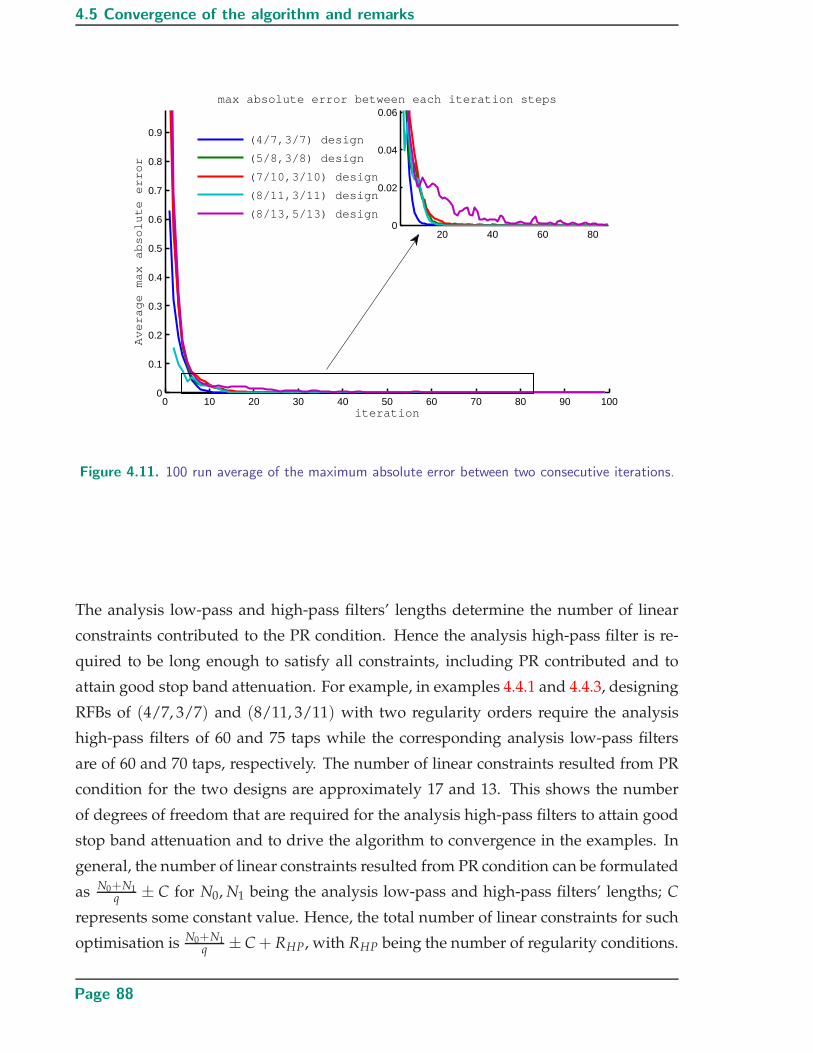
4.5 Convergence of the algorithm and remarks
0 10 20 30 40 50 60 70 80 90 1000
0.1
0.2
0.3
0.4
0.5
0.6
0.7
0.8
0.9
iteration
Ave
rag
e m
ax
ab
solu
te e
rro
r
max absolute error between each iteration steps
(4/7,3/7) design
(5/8,3/8) design
(7/10,3/10) design
(8/11,3/11) design
(8/13,5/13) design
20 40 60 800
0.02
0.04
0.06
Figure 4.11. 100 run average of the maximum absolute error between two consecutive iterations.
The analysis low-pass and high-pass filters’ lengths determine the number of linear
constraints contributed to the PR condition. Hence the analysis high-pass filter is re-
quired to be long enough to satisfy all constraints, including PR contributed and to
attain good stop band attenuation. For example, in examples 4.4.1 and 4.4.3, designing
RFBs of (4/7, 3/7) and (8/11, 3/11) with two regularity orders require the analysis
high-pass filters of 60 and 75 taps while the corresponding analysis low-pass filters
are of 60 and 70 taps, respectively. The number of linear constraints resulted from PR
condition for the two designs are approximately 17 and 13. This shows the number
of degrees of freedom that are required for the analysis high-pass filters to attain good
stop band attenuation and to drive the algorithm to convergence in the examples. In
general, the number of linear constraints resulted from PR condition can be formulated
as N0+N1q ± C for N0, N1 being the analysis low-pass and high-pass filters’ lengths; C
represents some constant value. Hence, the total number of linear constraints for such
optimisation is N0+N1q ± C + RHP, with RHP being the number of regularity conditions.
Page 88
Chapter 4 Bi-orthgonal RFB structure of (pq ,
q−pq ) - flexible Q factor transforms
In this chapter, we pre-designed analysis low-pass filter to approximate qth-band fil-
ters10. The PR condition (4.9) requires one of the q polyphase components of Qm(z) =
Fm(z)Hm(z) to be a pure delay, which implies that it must be an qth-band filter. By
choosing the pre-designed analysis low-pass filter to be an approximate qth-band filter,
the resulting Qm(z) is also an approximate qth-band filter for any analysis high-pass
filter hHP having a flat pass-band response in [ q−1q π, π]11. This increases the likelihood
of convergence since at each iteration step, the obtained hHPmin always approximates
the algorithm solution, i.e. the corresponding Qm(z) being a qth-band filter.
The iterative algorithm behaves similarly to the fixed point iteration method in which
solutions of a high order polynomial are computed based on an iterative linear equa-
tions. The high order constraint in this problem, expressed in (4.25) and denoted as
f (hHP) = 0 are rewritten as g(hHP) = hHP. The solution for the constraint is a fixed
point of g.
The iterative algorithm discussed in this section fails to converge for the case p1 > 3.
In the proposed iterative approach, the high order p1 constraints are relaxed to one
(i.e. linear constraints). The relaxation is performed in (4.26), (4.27). In (4.27), each
product term of the sum which results in p1-order nonlinear constraints are linearised
by setting p1 − 1 polyphase components of the analysis high-pass filter to constant, i.e.
equal to those of the previous iteration. Only one polyphase component is considered
as unknowns, which leads to the constraints becoming linear for each iteration step.
When p1 = 3, the third order PR constraints were relaxed to sum of 3 sets of linear
constraints with respect to the the three polyphase components of analysis high-pass
filter hHP. Each set of the linear constraints corresponds to Γlj[n] as in (4.27) for j =
p0, . . . , q − 1 representing the index of the unknown polyphase component. Hence,
for p1 > 3, such relaxation from high order constraints to linear leads to failure in
attaining the fixed point solution for the PR constraint of high order. For p1 > 3 the
error in (4.32) cannot be reduced sufficiently to satisfy the convergence condition. In
all our empirical studies with p1 > 3, the algorithm will find suitable filters (provided
they are of sufficient lengths) with reconstruction error of 10−5, despite not reaching
convergence. The precise value varies with the design parameters such as the filter
lengths and cut-off frequencies.
10qth-band filter is defined as filters with pass-band response in the region of [ k0πq , k1π
q ] for intergers
k0, k1; k0 < k1 ≤ q and one of its q-polyphase is a pure delay11Such frequency response relationship is a result of the alias free condition (4.8).
Page 89

4.6 Chapter summary
We propose in cases of In such cases p1 > 3 that only two polyphase components of
hHP out of p1 polyphases should be used as unknowns in each iteration step in dealing
with PR condition. Thus, (4.26) becomes:
Γl [n] =p0+1
∑j=p0
Γlj[n] = 0, (4.33)
for
Γlj[n] = ∑
ni∈Kn={Krn}r∈N
ar
{ p0−1
∏i=0
hi[ni]} q−1
∏i=p0,i 6=j
hl−1i [ni]hj[nj], (4.34)
Γlj[n] in this case only takes two values of j = p0, p0 + 1 which corresponds to the un-
knowns of first and second polyphase components of hHP whilst other polyphase com-
ponents in (4.33) are known from the solution of the previous step l − 1 (i.e. hl−1i [ni],
i = p0 + 2, · · · , q − 1 are known) . Other steps of the iterative algorithm remains the
same. Such limit of j values in (4.33) improves the likelihood of convergence since
the constraint is now relaxed from second order to first. However, at the same time we
limit the number of variables contributing to satisfy PR conditions (only two polyphase
components of hHP are used as variables for PR condition) which leads to longer anal-
ysis filter hHP required. Example 4.5.1 illustrates a case of p1 = 5, designed base on the
proposed modification.
Example 4.5.1. RFB (8/13, 5/13) with one regularity order is considered. Hence, p1 = 5
in this example. The filter lengths are 65, 110, dilation factor of 13/8 = 1.625. The designed
filters’ responses and the corresponding constructed wavelet functions are illustrated in Fig.
4.12.
4.6 Chapter summary
In this chapter, the design of bi-orthogonal two channel rational filter bank with ar-
bitrary re-sampling ratios and multiple regularity orders is proposed, which is a gen-
eralisation of that of chapter 3. Thus, it began with a discussion of the more general
conditions for imposing regularity on the filter bank structure. This enables the flexibil-
ity of quality factor Q in the resulting constant Q-transform or more general RADWTs.
Local optimisation method as discussed in section 3.3.1 can be applied for all design
parameters p0, p1, q that satisfy PR necessary conditions (2.1). Such method however
relies much on a line-search algorithm to solve the nonlinear constraint optimisation
Page 90

Chapter 4 Bi-orthgonal RFB structure of (pq ,
q−pq ) - flexible Q factor transforms
0 5 10 15 20 25−0.01
−0.005
0
0.005
0.01
0.015analysis wavelet
(a)0 0.2 0.4 0.6 0.8 1
−100
−80
−60
−40
−20
0
20analysis low−pass and high−pass filters
(b)ω ( ×π rad/sample)
dB
0 5 10 15 20 25 30 35 40 45−0.01
−0.005
0
0.005
0.01synthesis wavelet
(c)0 0.2 0.4 0.6 0.8 1
−100
−80
−60
−40
−20
0
20synthesis low−pass and high−pass filters
(d)ω ( ×π rad/sample)
dB
analysis high−passanalysis low−pass
synthesis high−passsynthesis low−pass
Figure 4.12. ( 813 , 5
13 ) RFB with one regularity order (modified iterative approach). Left panels:
Analysis (a) and Synthesis (c) wavelet functions, respectively. Right panels show
the analysis (b) and synthesis (d) low-pass and high-pass filters’ frequency response,
respectively.
problem, provided an approximate solution to the problem is pre-obtained to feed the
algorithm. Thus, for high order q constraints and long filters, the algorithm complex-
ity increases significantly. An iterative algorithm is proposed and presented in section
4.3.1. The algorithm decomposes the original nonlinear problem into a sequence of
quadratic problems with linear constraints. Even though proof of the convergence is
still an unsolved problem, we empirically investigated the iterative maximum error
between successive steps against random initialisations. It shows that the the algo-
rithm converges in less than 100 iterations in all design examples. Some experiments
to demonstrate the use of our designed RADWTs in applications such as denoising and
signal separations based on basis pursuit principle are presented in the next chapter.
Page 91

Page 92

Chapter 5
Biorthogonal RADWT:Applications and
discussions
THIS chapter explores some applications for the RADWT designs
presented in chapters 3 and 4. They apply to a wide variety of
real-world signals, including speech and chirp signals. These sig-
nals share one common aspect: their bi-orthogonal RADWT representations
are sparse. This property is exploited for denoising and signal separation
based on basis pursuit (Chen et al. 2001). The presented experimental re-
sults show the effectiveness of using bi-orthogonal RADWTs with dyadic
wavelet transforms to construct dictionary for the basis pursuit problem.
Signal separation on chirp signals and narrow band interferences are used
as illustrative examples of this technique.
Page 93

5.1 Introduction
5.1 Introduction
The topic of sparse signal representation has raised much interest from researchers
(Akcakaya and Tarokh 2008b, Gribonval and Nielsen 2003) due to its fruitful appli-
cation to areas such as signal compression and coding (Teschke 2007) which has en-
abled compact storage and rapid transmission of information. For example, if the sig-
nals to be compressed are known to have sparse representations in some transform
domain, then they can be expressed or approximated by a small number of compo-
nents in that domain. Many transform bases and frames have been used in search
of sparsity for signals of various classes. Examples include short time Fourier trans-
form (STFT), discrete cosine transform (DCT), wavelet transforms, . . . , etc. Recently,
Selesick (Selesnick 2011c) has adopted the RADWT in search for sparsity. It is expected
that signals of an oscillatory nature, such as EEG, and speech are well-suited for de-
composition into a dictionary containing low and high resonance components, which
corresponds to RADWTs of low and high quality factors Q, respectively (Bayram and
Selesnick 2009a, Selesnick 2011a). The transforms used in the existing literature are
redundant and based on non-FIR filters.
In this chapter, we attempt to take advantage of the bi-orthogonal RADWTs designed
in chapters 3 and 4 in attaining sparse representation of signals such as the TIMIT
speech dataset (Garofolo et al. 1993). Denoising of TIMIT speech using the bi-orthogonal
RADWT representation is presented, whose results are compared against other dyadic
wavelet transforms. It is followed by some signal separation based on the basis pur-
suit principle, and uses a dictionary constructed from a concatenation of critically-
sampled RADWTs of various Q factors. In the literature, over-complete RADWTs are
used for constructing dictionaries for signal separation/decomposition based on basis
pursuit. This was first investigated in (Selesnick 2011b), where it was termed resonance
based signal separation. Here we construct our dictionary based on critically-sampled
RADWTs in mixture with dyadic wavelet transforms to separate the oscillatory and
non-oscillatory components of signals. Detailed work is discussed in section 5.2.3. In
section 5.3, signal separation of chirp signals mixed with sinusoidal interferences is
discussed. Section 5.4 provides the concluding remarks and chapter summary.
Page 94
Chapter 5 Biorthogonal RADWT: Applications and discussions
5.2 Speech signal processing
The speech signals used for the experiments in this section are from a corpus of phone-
mically and lexically transcribed speech of American English speakers of different
sexes and dialects. The corpus is designed by Texas instruments and Massachusetts
Institute of Technology (TIMIT) for automatic speech recognition research.
5.2.1 Comparing sparsity measures of TIMIT speech signals
RADWTs can be advantageous in representing signals of an oscillatory nature due to
its flexible dilation factor over conventional dyadic wavelets. In assessing the suit-
ability of different signal representations, the sparsity of appropriate classes of signals
is usually a useful proxy for representational efficiency. Fundamentally, sparsity is a
measure of how much of a signal’s energy is packed into few coefficients. In this exper-
iment, we apply two sparsity measures reported in (Hurley and Rickard 2009), namely
GINI index and pq-mean (for p = 1, q = 3), on wavelet transformed speech signals.
The sparsity measures are chosen as they are shown to satisfy all criteria for effective
sparsity measures, as discussed by (Hurley and Rickard 2009). GINI index is defined
as
GINI = 1 − 2N
∑k=1
x[k]
‖x‖1
(N − k + 1/2
N
)
, (5.1)
where x[n] represents ordered data such that 0 ≤ x[1] ≤ x[2] ≤ . . . ≤ x[N]; pq-mean for
p = 1, q = 3 can be expressed as
pqmean = −( 1
N
N
∑k=1
x[k]) 1
3( 1
N
N
∑k=1
x[k]3)
, (5.2)
where x[n] ≥ 0 for n = 1, . . . , N. The considered signals are taken from the commonly
used TIMIT database (Garofolo et al. 1993) of phonemically and lexically transcribed
speech of American English speakers. The quantification is performed on a set of 100
TIMIT signals from both male and female speakers, being analysed by our RADWT
6/5 as it can approximate the psychoacoustic bark scale (Fastl and Zwicker 2007).
Comparisons are made with the dyadic wavelet transforms, db5 and db45, the orthog-
onal Daubechies wavelet of 5, 45 regularity orders, discrete Meyer wavelet dmey, a FIR
based approximation of the Meyer wavelet and bi-orthogonal spline wavelet with de-
composition and reconstruction regularity orders of 8 and 6, respectively (bior6.8).
Page 95

5.2 Speech signal processing
The choice of dyadic DWTs are made to be representative for different types of dyadic
wavelets. They include low and high regularity order DWTs and orthogonal and bi-
orthogonal DWTs. The discrete Meyer dmey is a dyadic DWT which uses filters with
good frequency selectivity.
The rational 6/5 discrete wavelet transforms are iterated for 15 levels, and all dyadic
wavelets are iterated for 4 levels, to equalise the range of resolutions captured by the
two transforms, since (56)
15 ≈ (12)
4. To take into account the sub-band energy gained
at each decomposition level due to the scale dependent norm of the designed RADWT,
the wavelets coefficients of each sub-band are multiplied by a compensation constant
defined as b � w; where w is the column vector representing the wavelets coefficients,
� denotes the element-wise multiplication of vectors b and w; b is defined to take
into account the scale dependent norm of the reconstruction wavelet functions such
that for any index k such that the coefficient w(k) corresponds to the weight of any
analysis wavelet function at level n0; ψn0 is the synthesis wavelet function at the same
level, defined by iterating the synthesis filters for n0 times; ‖.‖2 denotes the l2 norm.
The scale dependent norm adjustment is verified using Gaussian noise signals, where the
sparsity measures are compared between 4-level dyadic wavelet transforms, 15-level
RADWT 6/5 and untransformed data.
b[k] = ‖ψn0‖2 (5.3)
Fig. 5.1 illustrates the comparisons as the sparsity measures are approximately equal
between transformed and non-transformed noise data. One hundreds white Gaussian
noise signals of 0 mean and 1 variance is considered for the experiment. It should be
noted that, for white Gaussian noise signals, the representation sparsity should not
differ between transform and non-transform data. This is clearly shown in Fig. 5.1.
The sparsity measures comparison of speech signal dataset is illustrated in Fig. 5.2
and 5.3. In Fig. 5.2, RADWT 6/5 outperforms dyadic wavelet transformed and non-
transformed TIMIT signals, i.e. greater sparsity measures are attained for RADWT
coefficients. To better illustrate the distribution of sparsity measure for each wavelet
transform method, normalised histogram is constructed and shown in Fig. 5.3.
This experiment shows the RADWT 6/5 representation for TIMIT signals can achieve
better sparsity when compared with existing dyadic DWTs. The normalised histograms
in Fig. 5.3 shows RADWT coefficients distribute in greater value of sparsity measures
Page 96
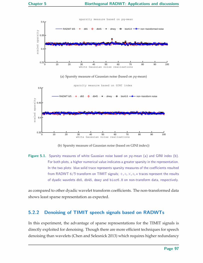
Chapter 5 Biorthogonal RADWT: Applications and discussions
0 10 20 30 40 50 60 70 80 90 1000.25
0.3
0.35
0.4
white Gaussian noise realisations
sparsity measure based on pq−mean
sca
led
sp
ars
ity
RADWT 6/5 db5 db45 dmey bior6.8 non−transformed noise
(a) Sparsity measure of Gaussian noise (based on pq-mean)
0 10 20 30 40 50 60 70 80 90 1000.35
0.4
0.45
0.5sparsity measure based on GINI index
sca
led
sp
ars
ity
white Gaussian noise realisations
RADWT 6/5 db5 db45 dmey bior6.8 non−transform noise
(b) Sparsity measure of Gaussian noise (based on GINI index))
Figure 5.1. Sparsity measures of white Gaussian noise based on pq-mean (a) and GINI index (b).
For both plots, a higher numerical value indicates a greater sparsity in the representation.
In the two plots: blue solid trace represents sparsity measures of the coefficients resulted
from RADWT 6/5 transform on TIMIT signals; +, ◦,×, �, ? traces represent the results
of dyadic wavelets db5, db45, dmey and bior6.8 on non-transform data, respectively.
as compared to other dyadic wavelet transform coefficients. The non-transformed data
shows least sparse representation as expected.
5.2.2 Denoising of TIMIT speech signals based on RADWTs
In this experiment, the advantage of sparse representations for the TIMIT signals is
directly exploited for denoising. Though there are more efficient techniques for speech
denoising than wavelets (Chen and Selesnick 2013) which requires higher redundancy
Page 97
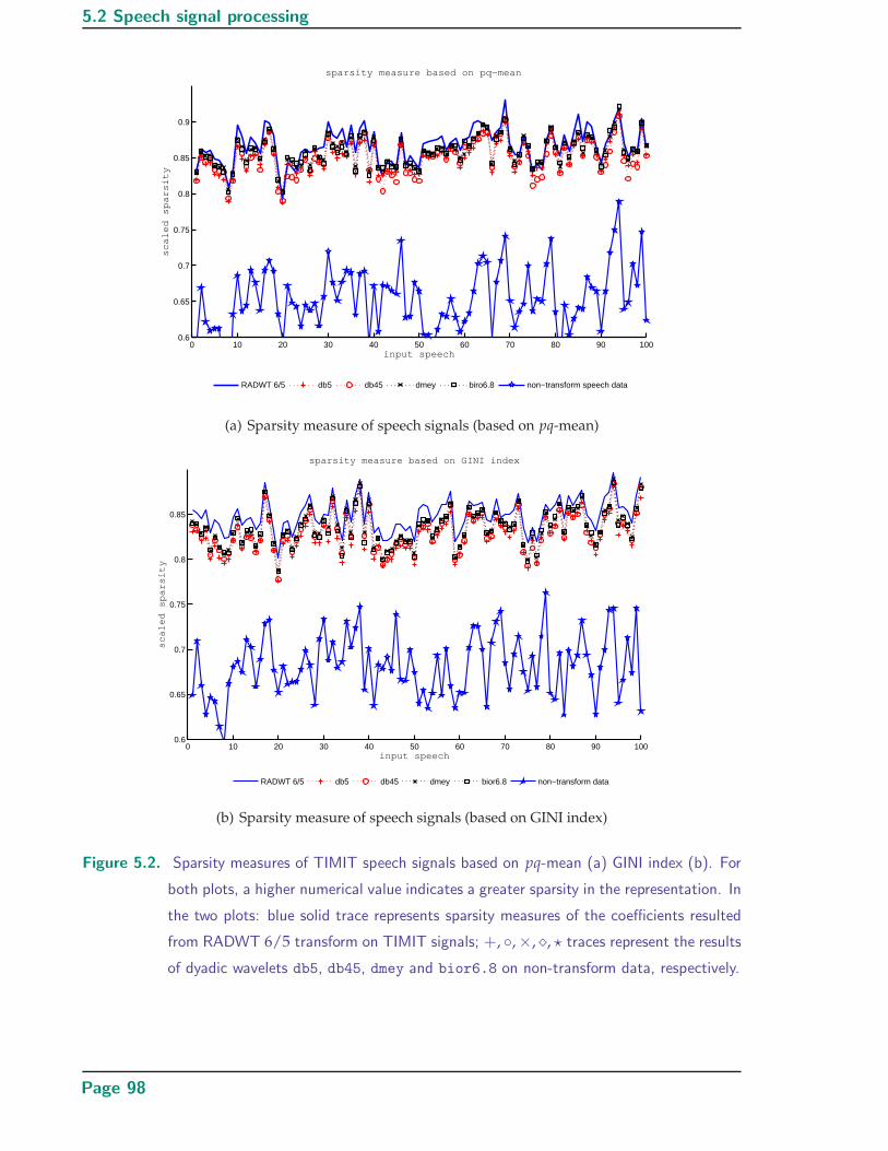
5.2 Speech signal processing
0 10 20 30 40 50 60 70 80 90 1000.6
0.65
0.7
0.75
0.8
0.85
0.9
input speech
sparsity measure based on pq−mean
sca
led
sp
ars
ity
RADWT 6/5 db5 db45 dmey biro6.8 non−transform speech data
(a) Sparsity measure of speech signals (based on pq-mean)
0 10 20 30 40 50 60 70 80 90 1000.6
0.65
0.7
0.75
0.8
0.85
input speech
sparsity measure based on GINI index
sca
led
sp
ars
ity
RADWT 6/5 db5 db45 dmey bior6.8 non−transform data
(b) Sparsity measure of speech signals (based on GINI index)
Figure 5.2. Sparsity measures of TIMIT speech signals based on pq-mean (a) GINI index (b). For
both plots, a higher numerical value indicates a greater sparsity in the representation. In
the two plots: blue solid trace represents sparsity measures of the coefficients resulted
from RADWT 6/5 transform on TIMIT signals; +, ◦,×, �, ? traces represent the results
of dyadic wavelets db5, db45, dmey and bior6.8 on non-transform data, respectively.
Page 98

Chapter 5 Biorthogonal RADWT: Applications and discussions
0.5 0.55 0.6 0.65 0.7 0.75 0.8 0.85 0.9 0.95 10
0.05
0.1
0.15
0.2
0.25
sparsity measure (pq−mean)
nomalised histogram of sparsity measure based on pq−mean
de
sity
RADWT 6/5 db5 db45 dmey bior6.8 non−transform data
(a) normalised histograms of the signals’ sparsity measure (pq mean)
0.5 0.55 0.6 0.65 0.7 0.75 0.8 0.85 0.9 0.95 10
0.05
0.1
0.15
0.2
0.25
sparsity measure (GINI index)
de
sity
nomalised histogram of sparsity measure based on GINI index
RADWT 6/5 db5 db45 dmey bior6.8 non−transform data
(b) normalised histograms of the signals’ sparsity measure (GINI index)
Figure 5.3. The normalised histograms of the signals’ sparsity measures. In the two plots: blue
solid trace represents sparsity measures of the coefficients resulted from RADWT 6/5
transform on TIMIT signals; +, ◦,×, �, ? traces represent the results of dyadic wavelets
db5, db45, dmey and bior6.8
transforms and computational complexity, the experiment simply compares RADWTs’
performance with other wavelet bases for denoising speech signals. The designed
RADWT with dilation factor 6/5 = 1.2 is again used since the bandwidths of the cor-
responding transform approximate the psychoacoustic Bark scale (Fastl and Zwicker
2007) to compare with conventional dyadic wavelets. Soft thresholding and Stein’s
Page 99

5.2 Speech signal processing
0 10 20 30 40 50 60 70 80 90 1004.5
5
5.5
6
6.5
7
7.5
8
8.5
input speech
Denoising result with input SNR of 0 dB
dB
RADWT 6/5 db5 db45 dmey bior6.8
(a) output SNR for 0 dB input SNR
0 10 20 30 40 50 60 70 80 90 1008
8.5
9
9.5
10
10.5
11
11.5
12
input speech
Denoising result with input SNR of 5 dB
dB
RADWT 6/5 db5 db45 dmey bior6.8
(b) output SNR for 5 dB input SNR
Figure 5.4. TIMIT speech signals denoising based on dyadic wavelet and RADWT 6/5 on 100
different input speech signals of input SNR of 0, 5 dB. In the two plots: blue solid
trace represents denoising result of RADWT 6/5; +, ◦,×, � dotted traces represent the
results of Daubechies wavelets db5, db45, dmey, bior6.8 respectively.
Page 100

Chapter 5 Biorthogonal RADWT: Applications and discussions
−1 −0.5 0 0.5 1 1.50
0.05
0.1
0.15
0.2
0.25
dB
Denoising gain for input SNR of 0 dB
de
nsi
ty
db5db45dmeybior6.8
(a) histogram of the denoising gain for 0 dB input SNR
−1 −0.5 0 0.5 1 1.50
0.02
0.04
0.06
0.08
0.1
0.12
0.14
0.16
0.18
0.2
dB
Denoising gain for input SNR of 5 dB
de
nsi
ty
db5db45dmeybior6.8
(b) histogram of the denoising gain for 5 dB input SNR
Figure 5.5. The normalised histograms of the denoising gain. In two plots: SNR of each input set
resulted from RADWT 6/5 is subtracted by the corresponding SNR of dyadic DWTs
db5 (solid blue), db45 (+ purple), dmey (◦ red) and bior6.8 (× black), respectively.
Top plot represents result of 0 dB input SNR while bottom corresponds to 5 dB input
SNR. Positive gain denotes superior performance by RADWT and vice versa.
unbiased risk estimate-SURE (Stein 1981) are used for denoising operation and to es-
timate the threshold value at each level of the wavelet decompositions, respectively.
These choices are empirically made to maximise the denoising performance. Other
schemes are also considered such as hard thresholding and other threshold estima-
tion techniques including fixed threshold estimate of√
2 log lx (Donoho and Johnstone
1994) with lx being the signal length and minimax threshold estimation (Donoho 1995).
Page 101

5.2 Speech signal processing
Amongst the techniques, soft thresholding with SURE threshold estimate was found to
give best SNR results. Hence, it is chosen for the denoising performance comparison.
The recovered signals’ SNR, which associate to mean-squared error (MSE), is the mea-
sure for comparison. One hundred noise realisations are used and the average MSE is
calculated for the final recovery signal SNR. Signals are corrupted by white Gaussian
noise of input speech SNR of 0, 5 dB. The wavelet transforms are computed for 15, 4
levels for RADWT 6/5 and dyadic transforms, respectively. The same set of TIMIT
signals as in experiment 1 is used for this experiment. The results are shown in Fig. 5.4,
which demonstrates the denoising improvement. This is a result of the sparser repre-
sentation property of RADWT 6/5 as compared to dyadic DWTs, shown in experiment
1. To better illustrate the difference in denoising SNR for each dataset, the denoising
SNR gain of RADWT compared to dyadic DWT is computed and defined as
Gdyad[i] = SNRRAD [i]− SNRdyad [i], (5.4)
where SNRRAD [i], SNRdyad [i] are the denoising output SNR of the RADWT and dyadic
DWT of the speech dataset index i = 1, . . . , 100, respectively, subscript dyad repre-
sents the name of the dyadic DWT that is compared with the RADWT. In Fig. 5.5,
normalised histogram of SNR difference Gdyad[i], i = 1, . . . , 100 between RADWT and
dyadic DWTs are illustrated. Note that the positive dB gain (Gdyad > 0) denotes the
superiority of RADWT over the dyadic DWT while negative gain shows otherwise.
From the figure, it could be noted that the maximum attained gain for 0, 5 dB input
SNR are 0.7, 1.05 dB while the worst cases show losses of 0.3, 0.5 dB, respectively. The
RADWT outperforms dyadic DWTs in 87% and 93% of the testing signals in cases of
0, 5 dB input SNR, respectively.
5.2.3 Speech signal decomposition
In this experiment we demonstrate the use of RADWTs in signal decomposition based
on the principle of basis pursuit. A speech signal is decomposed into separate oscil-
latory and non-oscillatory components for audio coding purpose, since such compo-
nents can be more effectively modeled/encoded by mixed Q decompositions (Molla
and Torrsani 2005). Similar decomposition is addressed in other papers in the liter-
ature (Levine 1998, Laurenti et al. 2007). In this thesis, the signals are decomposed
based on based on constant Q transforms constructed from the designed bi-orthogonal
RADWT.
Page 102

Chapter 5 Biorthogonal RADWT: Applications and discussions
In this experiment, our dictionary for the basis pursuit algorithm is constructed as a
concatenation of our design design critically sampled two regularity order RADWT
with dilation factor of 11/8 as reported in Example 3 of Sec. 4.4 and dyadic wavelet
db2. One segment of speech signal (the word “I’m” spoken by a male speaker) is ex-
perimented with in a similar fashion as described in (Selesnick 2011b), to facilitate
direct comparison. The resulting decomposition obtained is illustrated in Fig. 5.6. In
our decomposition, the dictionary’s redundancy is 2, which is much smaller than W.
and Selesnick’s. The decomposition is attained by finding minimal l1 norm solutions
for each wavelet representation as we optimise
minw1,w2
λ1‖b1 � w1‖1 + λ2 ‖b2 � w2‖1 subject to Φ−1dy w1 + Φ−1
RADw2 = s (5.5)
where Φdy, ΦRAD are the square matrices representing the non-redundant wavelet trans-
forms dyadic and RADWT 11/8, respectively; Φ−1dy , Φ−1
RAD denote their inverse trans-
form matrices. The transforms Φdy, ΦRAD in (5.5) are selected to be sufficiently in-
coherent. In other words, the analysis/synthesis functions of the two wavelets have
low correlation. The incoherence measure, defined as the maximum correlation be-
tween the wavelet functions from the two transforms, is proportional to the ratio be-
tween quality factors Q1, Q2 of the transforms Φdy, ΦRAD. The measure is defined as
(Selesnick 2011b)
ρ(Q1, Q2) =
√
Q1 + 1/2
Q2 + 1/2, Q2 > Q1, (5.6)
where Q1, Q2 are quality factors of the two transforms.
Wavelet decompositions are performed for 4 and 9 levels for dyadic and RADWT
11/8, respectively since (12)
4 ≈ ( 811)
9; w1, w2 represent wavelet coefficient vectors of
the dyadic transform and RADWT 11/8 , respectively; � represents the element-wise
multiplication of vectors b1, b2 and w1, w2, respectively; b1, b2 are the scale dependent
norms of the reconstruction wavelet functions, constructed as in (5.3); s is the original
speech signal; λ1, λ2 are scalar parameters, whose ratio determines the energy distri-
bution between the two wavelet transforms. The l1 minimisation problem in (5.5) is
solved using the iterative SALSA algorithm (Afonso et al. 2010, Selesnick 2011c). The
dyadic wavelet’s role is to pick up the transient non-oscillatory component, which ex-
hibits wide bandwidth and low Q factor characteristics while RADWT 11/8’s role is to
Page 103

5.2 Speech signal processing
0 0.02 0.04 0.06 0.08 0.1 0.12−0.4
−0.2
0
0.2
RADWT 11/8 − two regularity orders
0 0.02 0.04 0.06 0.08 0.1 0.12−0.5
0
0.5
1Dyadic db2, two regularity orders
0 0.02 0.04 0.06 0.08 0.1 0.12−0.5
0
0.5
1
Time (seconds)
speech signal Fs=16000 Hz
Figure 5.6. Speech signal decomposition (non-oscillatory and oscillatory components). Top panel
represents the non-oscillatory components (picked up by dyadic wavelets transform)
while middle panel shows the oscillatory part (picked up by the RADWT with dilation
factor of 11/8). Bottom is the original speech signal.
pick up the sustained oscillation counterpart of the signal, which exhibits narrow band-
width and high Q characteristics 12. It should be noted that in Fig. 5.6 middle panel,
the oscillatory component exists as high frequency before 0.095s and low frequency
after 0.095s. This suggests that as a result of the l1 minimisation in (5.5), the oscillatory
characteristics of the signal are extracted out and not a simple frequency domain sep-
aration. Autoregressive (AR) model is then applied to both the oscillatory component
and original speech signal for comparison. The signals are modeled with AR models,
whose parameters are computed using burg (Burg 1968, Brockwell et al. 2005) and co-
variance (Marple Jr 1987) methods, with the ratio between standard deviations of the
oscillatory component to original speech signal being 0.132 and a model order p = 6.
Hence, the prediction error rate attained is slightly better than the reported value in
the literature of 0.147, and with computational advantage of lower redundancy.
12In the extreme case, such two characteristics are the Dirac delta (non-oscillatory) and the sinusoidal
(purely oscillatory) functions
Page 104

Chapter 5 Biorthogonal RADWT: Applications and discussions
In this experiment, we re-produce the speech decomposition described in literature
(Selesnick 2011b) and demonstrate the use critically-sampled RADWT in signal sepa-
ration based on basis pursuit principle. Slight improvement in prediction error in our
case of 0.132 over the literature 0.147 with lower redundancy used for constructing
the dictionary can be attained. Besides, critically-sampled RADWT is more suitable
for use in conjunction with dyadic wavelet transforms in construction basis pursuit’s
dictionary. The dyadic wavelets possess various properties such as linear-phase (bi-
orthogonal), existing from low to very high regularity orders (Daubechies), good fre-
quency selectivity (discrete Meyer) which can be flexibly chosen for different types of
signals.
5.3 Chirp signal separation from narrow band interfer-
ence
5.3.1 Chirp signal separation from prolonged sinusoidal interference
The mixed Q signal separation in (5.5) can be applied for signal filtering, in situations
which pure frequency domain filtering cannot be applied. In the following, we con-
sider an example of a wide band signal interfered by narrow band sinusoids. Consider
signal s = sI + sS, where sI represents a low frequency sinusoidal interference with dis-
crete frequency ωd = .045π and sS is a real linear chirp with instantaneous frequency
ranging from [0, π]. We rewrite the equation (5.5) for this experiment as follows:
minwI,wS
λI‖bI � wI‖1 + λS ‖bS � wS‖1 subject to Φ−1S wS + Φ−1
I wI = s, (5.7)
where ΦS, ΦI are dyadic db1 DWT and RADWT 7/6, respectively. For such a mix-
ture, purely frequency based analysis cannot separate sI , sS since they reside in the
same frequency band at various times. Notch filter can possibly be used provided that
we have knowledge about the discrete frequency (ωd) and spectrum level of the sinu-
soid signal sI . However, the notch filtering can partially or completely remove that
frequency component from the original chirp signal. For unknown ωd, l1 minimisa-
tion, described in (5.7) can be used for the separation. The transforms’ decomposition
levels are 3 and 27, respectively. The time domain signal s and its spectrogram are il-
lustrated in Fig. 5.7 (a) and Fig. 5.8, respectively. The resulting separated signals are
illustrated in Fig. 5.7 (b), (c). In this experiment, the linear chirp behaves as a non-
Page 105

5.3 Chirp signal separation from narrow band interference
0 200 400 600 800 1000 1200 1400 1600 1800 2000−2
−1
0
1
2
Time (samples)
Linear chirp with low sine interference − SIR = 2.00 dB
(a) The original interfered chirp signal
200 400 600 800 1000 1200 1400 1600 1800 2000−1
−0.5
0
0.5
1
Chirp signal − picked up by Dyadic db1 − SNR = 12.80 dB
Time (samples)
400 450 500 550 600 650
−1
0
1
Time (samples)
reconstructed signal original signal
1620 1640 1660 1680 1700 1720 1740 1760−1
−0.5
0
0.5
1
Time (samples)
(b) Reconstructed chirp super-imposed with the original chirp signal
0 200 400 600 800 1000 1200 1400 1600 1800 2000−1.5
−1
−0.5
0
0.5
1
1.5Sinusoidal interference signal − picked up by 7/6 RADWT for SIR = 2.00 dB
Time (samples)
reconstructed signal original signal
(c) Reconstructed interference super-imposed with the original interfered sinusoid
Figure 5.7. From top to bottom of (a) are: original signal s (mixture of chirp and sinusoid signal);
(b) represents linear chirp signal and (c) is the sinusoid signal. Red dashed and solid blue
traces are original and the reconstructed signals for in both (b) and (c), respectively.
oscillatory component in the sense that its constant frequency oscillations exist over
infinitesimally short interval of time. It also exhibits wide bandwidth and low thus Q
characteristic, which explains why it was well represented by the dyadic wavelet. The
Page 106

Chapter 5 Biorthogonal RADWT: Applications and discussions
Figure 5.8. Spectrogram plot of signal s.
low frequency sinusoidal signal, on the other hand, has an oscillatory (high Q) char-
acteristic and is therefore captured by the RADWT. This technique can thus be used
to mitigate monochromatic interference at an unknown frequency. In this experiment,
Table 5.1. Reconstructed SNR versus SIR for linear chirp and prolonged sinusoidal signals separation
SIR −13 dB −8 dB −3 dB 2 dB
20 log10 (λIλS) 29.69 dB 35.04 dB 36.82 dB 38.56 dB
SNR 9.28 dB 10.6 dB 12.01 dB 12.80 dB
the choice of λI , λS of (5.7) is critical. These parameters vary depending on the input
signal to interference ratio. Various signal to interference ratios (SIR) are tested and the
recovered chirp signal to noise ratios (SNR) are computed. SIR is defined as the ratio of
the original chirp’s energy to the interference sinusoid’s. The noise energy is defined
as the square error between the original chirp signal and the reconstructed signal after
the separation. For each case of input SIR the ratio λI/λS is empirically selected to at-
tain optimal result of SNR. In table 5.1, the optimal resultant SNR versus input SIR and
ratio λI/λS are shown. The results show how optimal choices of λI/λS vary with the
input SIR. For example, greater SIR requires greater λI/λS ratio and vice versa which
agrees well with the expression (5.7), i.e. when the ratio λI/λS increases less energy is
distributed in wI (interference) while more energy is distributed in wS (signal).
Page 107

5.3 Chirp signal separation from narrow band interference
0 200 400 600 800 1000 1200 1400 1600 1800 2000−2
−1
0
1
2
Time (samples)
Linear chirp with low sine interference − SIR = 10.32 dB
(a) The original interfered chirp signal
200 400 600 800 1000 1200 1400 1600 1800 2000−1
−0.5
0
0.5
1
Chirp signal − picked up by Dyadic db1 − SNR = 14.64 dB
Time (samples)
reconstructed signal orginal signal
450 500 550 600 650
−1
−0.5
0
0.5
1
Time (samples)
reconstructed signal orginal signal
1560 1580 1600 1620 1640 1660
−1
0
1
Time (samples)
reconstructed signal orginal signal
(b) Reconstructed chirp super-imposed with the original chirp signal
0 200 400 600 800 1000 1200 1400 1600 1800 2000−1
−0.5
0
0.5
1
samples
reconstructed signal original signal
(c) Reconstructed short burst sinusoid super-imposed with the original interference
Figure 5.9. From top to bottom of (a) are: original signal s (mixture of chirp and sinusoid signal);
(b) represents linear chirp signal and (c) is the sinusoid signal. Red dashed and solid
blue traces are original and the reconstructed signals in both (b) and (c), respectively.
5.3.2 Chirp signal separation from short burst interference
As an extension of the previous experiment, we demonstrate in this experiment that
a similar separation can be effective for wide bandwidth linear chirps suffering inter-
ference by temporally sporadic monochromatic source. In this situation, the sinusoid
Page 108

Chapter 5 Biorthogonal RADWT: Applications and discussions
Figure 5.10. Spectrogram plot of signal s.
Table 5.2. Reconstructed SNR versus SIR for linear chirp and short burst sinusoid separation
SIR −4.68 dB 0.32 dB 5.32 dB 10.32 dB
20 log10 (λIλS) 29.86 dB 35.37 dB 39.58 dB 44.58 dB
SNR 8.00 dB 10.18 dB 12.28 dB 15.41 dB
signal corresponding to one discrete frequency, exists only in a short interval of time as
shown in Fig. 5.9 (c). The dictionary used for the signal separation consists of RADWT
7/6, and the dyadic db1.
The result illustrated in Fig. 5.9 (b) and (c) show that the RADWT can effectively extract
the temporal sinusoid signal component from the mixture with linear chirp of 10.32 dB
SIR to attain 14.64 dB output SNR. The decomposition levels are 27 and 3 for RADWT
7/6, and dyadic db1, respectively. The separated signals are plotted against their orig-
inal expected signals, both are illustrated in Fig. 5.9 (b) and (c). The spectrogram of
the original signal s is shown in Fig. 5.10. In table 5.2, the optimal resulted SNR versus
input SIR and ratio λI/λS are shown. Again, the ratio λI/λS is empirically selected
to attain optimal result SNR of each SIR case with some knowledge about the input
SIR. In this experiment, it is more apparent how the optimal λI/λS varies with respect
to the input SIR. It should be noted that the optimal ratio for 20 log10(λI/λS) differs
by approximately 5 dB from one case to the next, which equal to the difference in SIR
Page 109

5.3 Chirp signal separation from narrow band interference
Figure 5.11. Spectrogram plot of signal s.
between two consecutive test cases. It is because λI/λS determines the energy ratio of
the signal sI , sS resulting from the optimisation.
The experiments in section 5.3.1 and 5.3.2 show the effective separation of chirp signal
from the low frequency sinusoid interference. However, if the narrow bandwidth in-
terference is located in the middle or high frequency, the problem becomes more com-
plicated. It is because to separate such high Q factor interference, a corresponding high
Q RADWT is required. In the following, we present a similar separation with the nar-
row band interference locating approximately near the middle of the chirp bandwidth.
The non-oscillatory behavior of the linear chirp signal can be made more significant
by increasing the rate of frequency change over time, figure 5.11 illustrates the spectro-
gram of the analysed signal. The narrow band interference locating at near the middle
of the chirp bandwidth requires a more oscillatory type of RADWT to pick up, hence
the RADWT 11/10 of 3 regularity orders is used. The separation is shown in figure
5.12. It could be observed from figure 5.12 that the separation is possible in this case
of mid-band interference even though the output SNR attained is 9.2 dB for 8 dB SIR
which results in an approximate 4 dB loss compared to the low frequency short burst
Page 110

Chapter 5 Biorthogonal RADWT: Applications and discussions
0 200 400 600 800 1000 1200 1400 1600 1800 2000
−2
0
2
RADWT 11/10 (HIGH Q−TRANSFORM)
0 200 400 600 800 1000 1200 1400 1600 1800 2000−2
0
2Dyadic db20, dilation factor 2 (LOW Q−TRANSFORM)
100 200 300 400
−1
0
1
900 950 1000 1050 1100 1150 1200−2
0
2
850 900 950 1000 1050 1100 1150 1200
−2
0
2
RADWT 11/10 (HIGH Q−TRANSFORM)
reconstructed signal original signal
Figure 5.12. From top to bottom of are: original signal s (mixture of chirp and sinusoid signal);
zoomed in region of the reconstructed linear chirp; the narrow band interfered signal
and the zoomed in region of the narrow band interference. Red dashed and solid blue
traces are original and the reconstructed signals, respectively.
case. Further study should be done for this case of interference since a more suitable
transform should be used to extract the interference signal.
5.4 Concluding remarks and summary
From the experiments presented, we can summarise the key advantages of the RADWT
designs as follow:
Constant Q-transform or wavelet transform with flexible Q-RADWTs are better suited
to representing signals of an oscillatory nature with greater sparsity. This is shown in
section 5.2.1 for TIMIT speech signals, which benefited from the bi-orthogonal RADWT
Page 111

5.4 Concluding remarks and summary
6/5. Bi-orthogonal RADWTs can effectively be used to separate sustained oscilla-
tion components of signals from the non-oscillatory ones based on l1 minimisation
as in (5.5), where they are used with dyadic wavelets to form the problems’ dictionary.
In chirp signal separation experiments, basis pursuit problem with bi-orthogonal RADWT
and dyadic DWTs dictionary have shown some effectiveness in recovering linear chirp
signal from low frequency sinusoidal interference at an unknown frequency. How-
ever, the separation does not work in cases of high frequency sinusoidal interference
since very high Q-RADWT is required to sparsely represent such signal. More appro-
priate bases/frames are required for such cases of interference. Experiments on the
choices of λI/λS of (5.7) were considered. The results suggest that to find an optimal
choice λI/λS, knowledge of the input SIR is required. The effect of regularity orders
of the wavelets used in dictionary and the choice of decomposition levels are not yet
investigated in this thesis due to scope limiting. The choices made in the experiments
presented in this chapter are empirically based.
The experiments on chirp signal separation shows that such separation can be very
useful in reconstructing wide-band signals corrupted by narrow-band interference sources
which reside in the same frequency band. A similar demonstration was presented
in (Duarte et al. 2006), in which chirplet dictionary (Baraniuk and Jones 1993) and Fourier
basis were chosen to construct the incoherent bases dictionary. The presented method
is based on matching pursuit, hence greedy algorithm, as differed from basis pursuit as
presented in this paper, which can offer several advantages such as better sparsity and
super-resolution over matching pursuit (Chen et al. 1998). Note that the re-sampling
ratios of the RFB, and hence dilation factors, used in the basis pursuit algorithms are
chosen to ensure incoherence between the transforms in the dictionaries.
In this chapter, basis pursuit algorithm is adopted for the signal separation experiments
which allows inferring/separating signal in noiseless observations. However, in the
presence of noise and exact representation could not be obtained, l2-norm error can be
imposed. The optimization can be formulated as
minw
‖w‖1 subject to∥∥∥Φ−1w − x
∥∥∥
2
2≤ ε (5.8)
where ε is a positive real parameter representing the l2 penalty chosen in associa-
tion with the noise level; Φ is a N × M matrix representing a redundant dictionary
with M > N; (5.8) allows inferring w from the noisy observation as compared to
the noiseless counterpart Φ−1w = x. Note that though Φ−1 represents a matrix, the
Page 112

Chapter 5 Biorthogonal RADWT: Applications and discussions
matrix is not explicitly stored since it is costly and impractical in problems involving
long signals. However, the matrix-vector products Φ−1w can still be computed effi-
ciently. For example, if Φ, Φ−1 represent a dyadic wavelet transform and the inverse
transform matrices, a fast discrete wavelet and the inverse transform can be com-
puted without requiring the actual transform and inverse matrices. In solving (5.8)
(Figueiredo et al. 2007, Fuchs 2007), computation of the transposed matrix operation
Φ−1tw is required since the l2 penalty can be expanded to
∥∥∥Φ−1w − x
∥∥∥
2
2≤ ε (5.9)
⇔ (Φ−1w − x)t(Φ−1w − x) ≤ ε (5.10)
⇔ wtΦ−1tΦ−1w − wtΦ−1t
x − xtΦ−1w + xtx ≤ ε (5.11)
If Φ contains orthogonal bases or tight frames, the transposing operation simply in-
volves the inverse operation. For dictionaries consisting of non-tight frames, explicitly
defined matrix Φ−1 is required to compute its transposition. The proposed RADWTs
are non-tight frames, hence its use the in constructing the redundant dictionary of (5.8)
is limited to small scale problems when the stored and manipulated matrix can be
within reasonable computational resources.
Page 113

Page 114

Chapter 6
Thesis conclusion andfuture work
THIS chapter summarises the key findings of the thesis and poten-
tial direction for future work.
Page 115

6.1 Introduction
6.1 Introduction
Since the discovery of dyadic wavelet transforms, the available literature has been
dominated by studies on the construction of wavelet transforms from filter banks
with various properties. Recently, finer frequency decomposition resulting from it-
erated rational rate filter banks or rational discrete wavelets have drawn greater at-
tention. The rational structure leads to constant Q transforms whose Q factor is ad-
justable, which is a departure from conventional dyadic wavelets. The newly re-
ported transform bases (frames), termed RADWTs in this thesis, enrich the existing
bases in searching for sparse representation of signals from various classes. Represen-
tation sparsity is the key feature for many applications including compressive sens-
ing (Candes and Romberg 2007, Candes 2006, Candes and Wakin 2008), denoising
(Cands et al. 2008, Zhu 2008), signal separation (Selesnick 2010, O’Grady et al. 2005,
He et al. 2007, Tropp 2006, Rickard 2007, Yilmaz and Rickard 2004), or in image pro-
cessing (Mairal et al. 2008, Aharon and Elad 2008, Esther Leung et al. 2008), . . . etc.
Therefore, the design of rational discrete wavelet transforms has been addressed by
many authors. The literature works are also categorised based on their approaches.
This thesis investigates bi-orthogonal rational discrete wavelets, which has not been
studied in the literature of RADWTs design. The resultant RADWTs are experimented
with signals of oscillatory nature, which show encouraging results in applications such
as signal coding and separation.
6.2 Thesis summary conclusion
In chapter 1, some background of time-frequency analysis and wavelet transform is
discussed together with the motivation for developing rational dilation factor wavelets.
The key issues to be addressed and contributions of the thesis are summarised.
In chapter 2, the design challenges of iterated rational FBs are discussed. The challenges
prevent the iterated rational rate filter banks from behaving as the conventional dyadic
transforms do in terms of multi-resolution analysis. Remedies for the issues are pro-
vided in this chapter. Necessary conditions for feasible FB parameters are provided
and the literature works of designing iterated RFBs and their key features are outlined.
Hence, the design challenges and research gap are underlined.
In chapter 3, a design of bi-orthogonal RFB with re-sampling rate satisfying ( q−1q , 1
q )
and multiple regularity orders is proposed. The issue of imposing regularity orders
Page 116

Chapter 6 Thesis conclusion and future work
on an bi-orthogonal structure is addressed. Two methods of solving the nonlinear
constraint optimisation, which arises from the FB design problem, are proposed with
some design examples.
In chapter 4, a design of bi-orthogonal RFB with re-sampling rate satisfying more gen-
eral p, q parameters (pq ,
q−pq ) is discussed with proof for imposing generalised regu-
larity conditions for arbitrary p, q pair. An iterative procedure for solving the design
problem is proposed, some design examples are provided. Mathematical proof for
convergence of the iterative algorithm though is not addressed, empirical evidence
and the affected factors to convergence of the algorithm are discussed.
In chapter 5, experiments on TIMIT and chirp signals using the designed bi-orthogonal
RADWTs are investigated. Some sparsity advantage is shown by using the bi-orthogonal
RADWTs for signals of oscillatory nature. Hence, the designed bi-orthogonal RADWTs
can be used with dyadic wavelet in constructing incoherent dictionary for applications
such as signal separation of chirp signals and narrow band interference.
6.3 Potential future work
In section 5.2, the proposed RADWTs and conventional dyadic wavelet transforms are
concatenated to form a redundant dictionary for a basis pursuit problem, in which exact
representation Φ−1w = x is imposed as the linear constraints of the optimisation prob-
lem (5.5). However, a more flexible optimisation, which allows some l2-norm error as
in (5.8) can overcome the potential issue of ill-conditioned or singular matrix Φj, which
arises in cases of exact representation Φ−1w = x (Figueiredo et al. 2007). There have
been many works investigating (5.8) in the literature including basis pursuit denoising
(Chen et al. 2001), regression shrinkage and selection via the lasso (Tibshirani 1996), whose
applications vary from signal reconstruction (Elad et al. 2006, Figueiredo and Nowak
2003, Figueiredo and Nowak 2005) to compressive sensing (Candes et al. 2006, Candes
and Tao 2006). Hence, a potential direction for future work is to attain a tight-frame
bi-orthogonal RADWTs. This will enable the use of RADWTs in problem as in (5.8) in
seeking the spareness of signal representation in the presence of noise.
The signals in the presented experiments are one dimensional signals. In image and
video coding, the spatial scalability factors for broadcasting applications is increasingly
in demand. Hence, the adjustable re-sampling property of the proposed bi-orthogonal
can be applied to increase the scalability of images, some relevant works are reported
Page 117

6.4 Original contributions
in (Pau et al. 2006). Fractional scalability is important for aspects such as ratio adaption
between wide-screen video formats. Besides, compressive sensing application using
the designed RADWTs in images can be a topic of investigation, which can be applied
in video coding.
6.4 Original contributions
We first provide a comprehensive summary of all design approaches to date regarding
RADWT designs. From the summary and key features, the gap is found and hence the
proposed design of bi-orthogonal RFB with multiple regularity orders. To achieve finer
frequency decomposition as compared to existing dyadic wavelets is the primary mo-
tivation of the RADWTs. Thus, a design of RFB satisfying (q−1
q , 1q ) is proposed, which
maximises such fine decomposition property for a given integer parameter q. Flexibly
adjusted Q factor, which is required to seek representation sparsity of many classes of
signals, results in (pq ,
q−pq ) RFB with more general parameters p, q being investigated.
Thus, a general proposition of imposing regularity orders for the bi-orthogonal RFB is
presented. The RFB design problem is formulated as a nonlinear constraint optimisa-
tion. Three approaches are proposed to solve such problem including linearised method,
local optimisation method and iterative method.
• The first one, attains solution in two steps, each of which is to solve a quadratic
problem with linear constraints. However, this approach only works for the de-
sign with p = 1.
• The second approach, local optimisation is applicable for all values p, q though
running time increases significantly as q increases since it determines the highest
order of the nonlinear constraints.
• The third approach solves the nonlinear constraint problem based on an iterative
procedure. Proof of convergence was not addressed in the thesis even though
extensive experiments of design examples suggest that the iterative algorithm
converges in less that 100 iterations. The factors that affect convergence of the
algorithm is discussed in section 4.5.
Finally, some application experiments inspired by the designed filters are presented to
illustrate their uses.
Page 118
Chapter 6 Thesis conclusion and future work
6.5 In closing
The chapter summarises the key contributions of the thesis and suggesting directions
for future work. The thesis investigates on bi-orthogonal rational rate filter banks with
regularity orders, which fills in the gap in the area of designing iterated RFB. The ad-
vantages and disadvantages of the designs are compared against the existing designs.
Together with the application experiments, the thesis has made contributions towards
enriching the existing time-frequency transform bases (frames) in seeking representa-
tions sparsity, which promotes a property which can potentially benefit many applica-
tions in the field of signal processing.
Page 119

Page 120

Appendix A
THIS chapter presents proof of some claims and propositions from
chapter 3 and 4.
Page 121

A.1 Detailed derivation of the regularity condition relationship
A.1 Detailed derivation of the regularity condition rela-
tionship
Proof. Re-writing equation (3.18), we have
F(z) = det A−(0,0)(zq−1)− z−q det A−(0,1)(z
q−1) + · · ·++ z−q(q−2)(−1)q−2 det A−(0,q−2)(z
q−1), (A.1)
A is the AC matrix, defined as in (3.15); A−(0,k)(zq−1) is a q − 1× q − 1 matrix, defined
as matrix A with row 0 and column k being removed. We replace A−(0,k) by Ak for
k = 0, · · · , q − 1, apply Laplace’s formula to the matrix determinants and re-arrange
the factors, we have the followings:
F(z) = (−1)(q−2)Hq−1(zq−1W)
[
det A0−(0,q−2) − z−q det A1−(0,q−2) + . . . + (−1)(q−2)×
z−q(q−2) det Aq−2−(0,q−2)
]
+ (−1)(1+q−2)Hq−1(zq−1W2)
[
det A0−(1,q−2)−
zq det A1−(1,q−2) + . . . + (−1)(q−2)z−q(q−2) det Aq−2−(1,q−2)
]
+ . . .+
(−1)(2q−4)Hq−1(zq−1Wq−1)
[
det A0−(q−2,q−2) − z−q det A1−(q−2,q−2) + . . .
+ (−1)(q−2)z−q(q−2) det Aq−2−(q−2,q−2)
]
. (A.2)
If we define the matrix
B =
z0q H0(zq−1W) z1qH1(zq−1W) · · · z(q−2)qHq−2(zq−1W)
......
......
z0qH0(zq−1Wq−1) z1q H1(zq−1Wq−1) · · · z(q−2)qHq−2(zq−1Wq−1)
, (A.3)
while the matrix C in (3.20) can be rewritten as
C =
H(zWq−1) H(zWq−1Wp) · · · H(zWq−1Wq−2p )
H(zWq−2) H(zWq−2Wp) · · · H(zWq−2Wq−2p )
......
......
H(zW) H(zWWp) · · · H(zWWq−2p )
, (A.4)
for W = ej2π/q, Wp = ej2π/(q−1). The following relationship can therefore be derived
in matrix forms as
B
1 1 1 · · · 1
1 Wp W2p · · · W
(q−2)p
......
......
...
1 W(q−2)p W
2(q−2)p · · · W
(q−2)(q−2)p
= C
Page 122

Appendix A
and
det Bc = det C, (A.5)
where c = det
1 1 1 · · · 1
1 Wp W2p · · · W
(q−2)p
......
......
...
1 W(q−2)p W
2(q−2)p · · · W
(q−2)(q−2)p
.
However, det B =
det
z0qH0(zq−1W) + · · ·+ · · · z(q−2)q×z(q−2)qHq−2(zq−1W) Hq−2(zq−1W)
......
...
z0qH0(zq−1Wq−1) + · · ·+ · · · z(q−2)q×z(q−2)qHq−2(zq−1Wq−1) Hq−2(zq−1Wq−1)
︸ ︷︷ ︸
first column of B is replaced by sum of all B’s columns
(A.6)
From (A.5), we have
(q − 1)det Bc = (q − 1)× det C (A.7)
Substitute (A.6) into the LHS of (A.7), we have
LHS =
c
det
H(zW(q−1)) · · · z(q−2)qHq−2(zq−1W)
......
...
H(zW) · · · z(q−2)qHq−2(zq−1Wq−1)
+ det
z0qH0(zq−1W) H(zW(q−1)) · · ·
......
...
z0qH0(zq−1Wq−1) H(zW) · · ·
+ · · ·
+ det
z0qH0(zq−1W) · · · H(zW(q−1))
......
...
z0qH0(zq−1Wq−1) · · · H(zW)
= (−1)0H(zW(q−1))[
zk0 det A0−(0,q−2) − zk0−q det A1−(0,q−2) + · · ·+
(−1)q−2zk0−q(q−2) det Aq−2−(0,q−2)
]
+ · · ·+ (−1)q−2H(zW)×[
zkn det A0−(q−2,q−2) − zkn−q det A1−(q−2,q−2) + · · ·+
(−1)q−2zkn−q(q−2) det Aq−2−(q−2,q−2)
]
Page 123

A.2 Relationship between filter’s polyphase component and its passband flatness
while
RHS = (q − 1)×[
H(zW(q−1))det C−(0,0) − H(zW(q−2))det C−(1,0)
+ · · ·+ (−1)q−2H(zW)det C−(q−2,0)
]
Equate LHS to RHS, we obtain
det C−(0,0) =c
q−1zk0[
det A0−(0,q−2) + · · ·+(−1)q−2z−q(q−2) det Aq−2−(0,q−2)
]
det C−(1,0) =c
q−1zk1[
det A0−(1,q−2) + · · ·+(−1)q−2z−q(q−2) det Aq−2−(1,q−2)
]
...
det C−(q−2,0) =c
q−1zkq−2[
det A0−(q−2,q−2) + · · ·+(−1)q−2z−q(q−2) det Aq−2−(q−2,q−2)
]
(A.8)
Substitute (A.8) into (A.2), we can find
F(z) =q − 1
c
[z−k0(−1)(q−2)Hq−1(z
q−1W)det C−(0,0)
+ z−k1(−1)(1+q−2)Hq−1(zq−1W2)det C−(1,0) + · · ·
+ z−kq−2(−1)(2q−4)Hq−1(zq−1Wq−1)det C−(q−2,0)
](A.9)
A.2 Relationship between filter’s polyphase component
and its passband flatness
Figure A.1. The filter H(z) and its frequency shifts magnitude response
Page 124
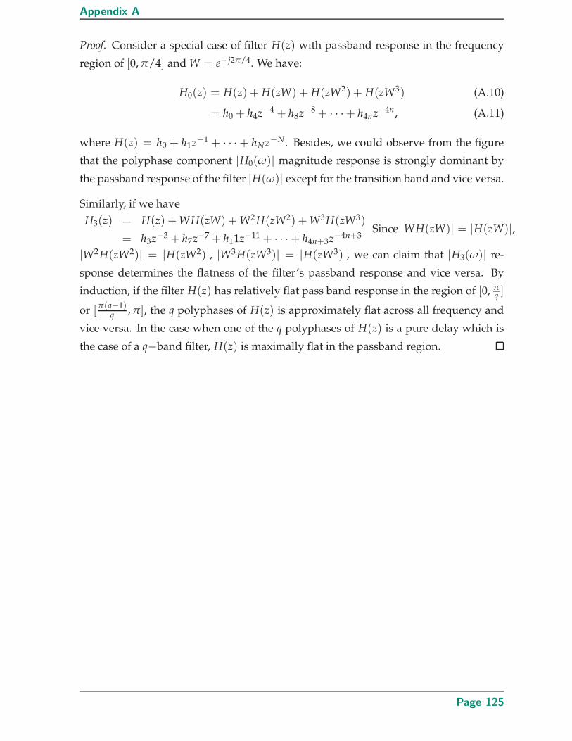
Appendix A
Proof. Consider a special case of filter H(z) with passband response in the frequency
region of [0, π/4] and W = e−j2π/4. We have:
H0(z) = H(z) + H(zW) + H(zW2) + H(zW3) (A.10)
= h0 + h4z−4 + h8z−8 + · · ·+ h4nz−4n, (A.11)
where H(z) = h0 + h1z−1 + · · ·+ hNz−N. Besides, we could observe from the figure
that the polyphase component |H0(ω)| magnitude response is strongly dominant by
the passband response of the filter |H(ω)| except for the transition band and vice versa.
Similarly, if we have
H3(z) = H(z) + WH(zW) + W2H(zW2) + W3H(zW3)
= h3z−3 + h7z−7 + h11z−11 + · · ·+ h4n+3z−4n+3Since |WH(zW)| = |H(zW)|,
|W2H(zW2)| = |H(zW2)|, |W3H(zW3)| = |H(zW3)|, we can claim that |H3(ω)| re-
sponse determines the flatness of the filter’s passband response and vice versa. By
induction, if the filter H(z) has relatively flat pass band response in the region of [0, πq ]
or [π(q−1)
q , π], the q polyphases of H(z) is approximately flat across all frequency and
vice versa. In the case when one of the q polyphases of H(z) is a pure delay which is
the case of a q−band filter, H(z) is maximally flat in the passband region.
Page 125

Page 126

Appendix B
Filter design results
THE appendix shows the responses of the designed filters that are
mentioned in the thesis whose responses yet to be shown.
Page 127

B.1 RFB designed by linearised method with parameters satisfying (q−1
q , 1q )
B.1 RFB designed by linearised method with parameters
satisfying (q−1q , 1
q)
Table B.1. The filter design parameters for appendices B.1.1-B.1.4.
Linearised method
B.1.1 parameters: B.1.2 parameters: B.1.3 parameters B.1.4 parameters
(2/3, 1/3), K = 2 (3/4, 1/4), K = 2 (6/7, 1/7), K = 4 (9/19, 1/10), K = 3
n0, L0, N0 42, 17, 35 50, 17, 33 63, 33, 65 96, 40, 79
N1 50 52 35 40
εLP εLP = 0 εLP = 0 εLP = 0 εLP = 0
ωsLP, ωsHP 0.388π, 0.592π 0.29π, 0.695π 0.193π, 0.787π 0.12π, 0.82π
where n0 determines the system’s delay, N0, N1 are the analysis low-pass and high-pass
filters’ lengths, respectively; L0, L1 are the mid-point indices of the analysis low-pass
and high-pass filters. If εLP = 0, it is equivalent that the pre-designed analysis low-
pass filter is an qth-band filter.
B.1.1 Rational filter bank of (23 , 1
3)
RFB of (23 , 1
3) with two regularity orders are designed based on linearised method. The
analysis low-pass and high-pass filters are of 35, 50 taps, respectively. The responses
are shown in Fig. B.1
B.1.2 Rational filter bank of (34, 1
4)
RFB of (34 , 1
4) with two regularity orders are designed based on linearised method. The
analysis low-pass and high-pass filters are of 33, 52 taps, respectively. The responses
are shown in Fig. B.2
B.1.3 Rational filter bank of (67 , 1
7)
RFB of (67 , 1
7) with four regularity orders are designed based on linearised method. The
analysis low-pass and high-pass filters are of 65, 35 taps, respectively. The responses
are shown in Fig. B.3
Page 128

Appendix B Filter design results
8 10 12 14 16 18 20
−0.01
−0.005
0
0.005
0.01
analysis wavelet
(a)0 0.2 0.4 0.6 0.8 1
−100
−80
−60
−40
−20
0
20analysis low−pass and high−pass filters
dB
(b)ω ( ×π rad/sample)
10 15 20 25 30 35 40
−5
0
5
x 10−3 synthesis wavelet
(c)0 0.2 0.4 0.6 0.8 1
−100
−80
−60
−40
−20
0
20synthesis low−pass and high−pass filters
dB
(d)ω ( ×π rad/sample)
analysis high−pass analysis low−pass
synthesis high−pass synthesis low−pass
Figure B.1. ( 23 , 1
3) RFB with two regularity orders. Left panels: Analysis (a) and Synthesis (c)
wavelet functions, respectively. Right panels show the analysis (b) and synthesis (d)
low-pass and high-pass filters’ frequency response, respectively.
2 3 4 5 6 7 8 9 10
−0.015
−0.01
−0.005
0
0.005
0.01
0.015
analysis wavelet
(a)0 0.2 0.4 0.6 0.8 1
−100
−80
−60
−40
−20
0
20analysis low−pass and high−pass filters
dB
(b)ω ( ×π rad/sample)
5 6 7 8 9 10 11 12 13 14
−0.01
−0.005
0
0.005
0.01
0.015synthesis wavelet
(c)0 0.2 0.4 0.6 0.8 1
−100
−80
−60
−40
−20
0
20synthesis low−pass and high−pass filters
dB
(d)ω ( ×π rad/sample)
analysis high−passanalysis low−pass
synthesis high−passsynthesis low−pass
Figure B.2. ( 34 , 1
4) RFB with two regularity orders. Left panels: Analysis (a) and Synthesis (c)
wavelet functions, respectively. Right panels show the analysis (b) and synthesis (d)
low-pass and high-pass filters’ frequency response, respectively.
Page 129
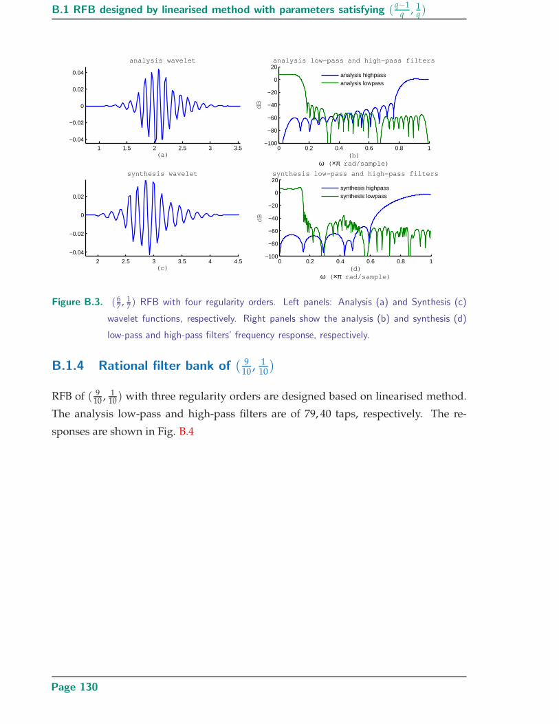
B.1 RFB designed by linearised method with parameters satisfying (q−1
q , 1q )
1 1.5 2 2.5 3 3.5
−0.04
−0.02
0
0.02
0.04
analysis wavelet
(a)0 0.2 0.4 0.6 0.8 1
−100
−80
−60
−40
−20
0
20analysis low−pass and high−pass filters
dB
(b)ω ( ×π rad/sample)
2 2.5 3 3.5 4 4.5
−0.04
−0.02
0
0.02
synthesis wavelet
(c)0 0.2 0.4 0.6 0.8 1
−100
−80
−60
−40
−20
0
20synthesis low−pass and high−pass filters
dB
(d)ω ( ×π rad/sample)
analysis highpassanalysis lowpass
synthesis highpasssynthesis lowpass
Figure B.3. ( 67 , 1
7) RFB with four regularity orders. Left panels: Analysis (a) and Synthesis (c)
wavelet functions, respectively. Right panels show the analysis (b) and synthesis (d)
low-pass and high-pass filters’ frequency response, respectively.
B.1.4 Rational filter bank of ( 910
, 110)
RFB of ( 910 , 1
10) with three regularity orders are designed based on linearised method.
The analysis low-pass and high-pass filters are of 79, 40 taps, respectively. The re-
sponses are shown in Fig. B.4
Page 130

Appendix B Filter design results
0.2 0.4 0.6 0.8 1 1.2 1.4 1.6
−0.04
−0.03
−0.02
−0.01
0
0.01
0.02
0.03
analysis wavelet
(a)0 0.2 0.4 0.6 0.8 1
−100
−80
−60
−40
−20
0
20analysis low−pass and high−pass filters
(b) ω ( ×π rad/sample)
dB
analysis low−passanalysis high−pass
6.2 6.4 6.6 6.8 7
−0.04
−0.02
0
0.02
0.04synthesis wavelet
(c)0 0.2 0.4 0.6 0.8 1
−100
−80
−60
−40
−20
0
20synthesis low−pass and high−pass filters
(d) ω ( ×π rad/sample)
dB
synthesis low−passsynthesis high−pass
Figure B.4. ( 910 , 1
10) RFB with three regularity orders. Left panels: Analysis (a) and Synthesis (c)
wavelet functions, respectively. Right panels show the analysis (b) and synthesis (d)
low-pass and high-pass filters’ frequency response, respectively.
Page 131

Page 132
Bibliography
AFONSO-M., BIOUCAS-DIAS-J., AND FIGUEIREDO-M. (2010). A fast algorithm for the constrained for-
mulation of compressive image reconstruction and other linear inverse problems, Acoustics Speech
and Signal Processing (ICASSP), 2010 IEEE International Conference on, pp. 4034 –4037.
AHARON-M., AND ELAD-M. (2008). Sparse and redundant modeling of image content using an image-
signature-dictionary, SIAM Journal on Imaging Sciences, 1(3), pp. 228–247.
AKCAKAYA-M., AND TAROKH-V. (2008a). A frame construction and a universal distortion bound for
sparse representations, Signal Processing, IEEE Transactions on, 56(6), pp. 2443–2450.
AKCAKAYA-M., AND TAROKH-V. (2008b). A frame construction and a universal distortion bound for
sparse representations, Signal Processing, IEEE Transactions on, 56(6), pp. 2443–2450.
AMIN-M., AND FENG-K. D. (1995). Short-time fourier transforms using cascade filter structures, Cir-
cuits and Systems II: Analog and Digital Signal Processing, IEEE Transactions on, 42(10), pp. 631
–641.
ANTONIADIS-A. (1997). Wavelets in statistics: A review, Statistical Methods & Applications, 6, pp. 97–
130. 10.1007/BF03178905.
ANTONINI-M., BARLAUD-M., MATHIEU-P., AND DAUBECHIES-I. (1992). Image coding using wavelet
transform, Image Processing, IEEE Transactions on, 1(2), pp. 205 –220.
ARGENTI-F., AND DEL RE-E. (1998). Rational sampling filter banks based on IIR filters, Signal Process-
ing, IEEE Transactions on, 46(12), pp. 3403 –3408.
AUSCHER-P. (1992). Wavelet bases for l2(r) with rational dilation factor, Wavelets and their applications,
Jones and Barlett, Boston, MA, USA, pp. 439–451.
BARANIUK-R. G., AND JONES-D. L. (1993). Shear madness: New orthonormal bases and frames using
chirp functions, IEEE Transactions on Signal Processing, 41(12), pp. 3543–3549.
BAUSSARD-A., NICOLIER-F., AND TRUCHETET-F. (2004). Rational multiresolution analysis and fast
wavelet transform: application to wavelet shrinkage denoising, Signal Processing, 84(10), pp. 1735–
1747.
BAYRAM-I., AND SELESNICK-I. (2009a). Frequency-domain design of overcomplete rational-dilation
wavelet transforms, Signal Processing, IEEE Transactions on, 57(8), pp. 2957 –2972.
BAYRAM-I., AND SELESNICK-I. W. (2007). Design of orthonormal and overcomplete wavelet transforms
based on rational sampling factors, Wavelet Applications in Industrial Processing V, Vol. 6763,
SPIE, Boston, MA, USA, pp. 67630H–15.
BAYRAM-I., AND SELESNICK-I. W. (2009b). Orthonormal FBs with rational sampling factors and over-
sampled DFT-modulated FBs: A connection and filter design, Signal Processing, IEEE Transactions
on, 57(7), pp. 2515–2526.
Page 133

Bibliography
BAYRAM-I., AND SELESNICK-I. W. (2009c). Overcomplete discrete wavelet transforms with rational
dilation factors, Signal Processing, IEEE Transactions on, 57(1), pp. 131–145.
BELOVA-N. Y., MIHAYLOV-S. V., AND PIRYOVA-B. G. (2007). Wavelet transform: A better approach for
the evaluation of instantaneous changes in heart rate variability, Autonomic Neuroscience, 131(1),
pp. 107–122.
BLU-T. (1993). Iterated filter banks with rational rate changes connection with discrete wavelet trans-
forms, Signal Processing, IEEE Transactions on, 41(12), pp. 3232–3244.
BLU-T. (1998). A new design algorithm for two-band orthonormal rational filter banks and orthonormal
rational wavelets, Signal Processing, IEEE Transactions on, 46(6), pp. 1494–1504.
BLU-T., DRAGOTTI-P.-L., VETTERLI-M., MARZILIANO-P., AND COULOT-L. (2008). Sparse sampling of
signal innovations, Signal Processing Magazine, IEEE, 25(2), pp. 31–40.
BREGOVIC-R., LIM-Y. C., AND SARAMAKI-T. (2008). Frequency-response masking-based design of
nearly perfect-reconstruction two-channel FIR filterbanks with rational sampling factors, Circuits
and Systems I: Regular Papers, IEEE Transactions on, 55(7), pp. 2002 –2012.
BROCKWELL-P. J., DAHLHAUS-R., AND TRINDADE-A. A. (2005). Modified burg algorithms for multi-
variate subset autoregression, Statistica Sinica, 15(1), pp. 197–213.
BURG-J. P. (1968). A new analysis technique for time series data, NATO Advanced Study Institute on
Signal Processing with Emphasis on Underwater Acoustics, pp. 12–23.
CANDES-E., AND ROMBERG-J. (2007). Sparsity and incoherence in compressive sampling, Inverse prob-
lems, 23(3), p. 969.
CANDES-E., AND WAKIN-M. (2008). An introduction to compressive sampling, Signal Processing Mag-
azine, IEEE, 25(2), pp. 21 –30.
CANDES-E. J. (2006). Compressive sampling, Proceedings oh the International Congress of Mathemati-
cians: Madrid, August 22-30, 2006: invited lectures, pp. 1433–1452.
CANDES-E. J., AND TAO-T. (2006). Near-optimal signal recovery from random projections: Universal
encoding strategies?, Information Theory, IEEE Transactions on, 52(12), pp. 5406–5425.
CANDES-E. J., ROMBERG-J. K., AND TAO-T. (2006). Stable signal recovery from incomplete and inaccu-
rate measurements, Communications on pure and applied mathematics, 59(8), pp. 1207–1223.
CANDS-E., WAKIN-M., AND BOYD-S. (2008). Enhancing sparsity by reweighted l1 minimization, Jour-
nal of Fourier Analysis and Applications, 14, pp. 877–905. 10.1007/s00041-008-9045-x.
CHEN-P.-Y., AND SELESNICK-I. W. (2013). Translation-invariant shrinkage/thresholding of group
sparse signals.
CHEN-S. S., DONOHO-D. L., AND SAUNDERS-M. A. (1998). Atomic decomposition by basis pursuit,
SIAM journal on scientific computing, 20(1), pp. 33–61.
CHEN-S. S., DONOHO-D. L., AND SAUNDERS-M. A. (2001). Atomic Decomposition by Basis Pursuit,
SIAM Review, 43, pp. 129–159.
Page 134

Bibliography
CHEN-W., KEHTARNAVAZ-N., AND SPENCER-T. (1993). An efficient recursive algorithm for time-
varying fourier transform, Signal Processing, IEEE Transactions on, 41(7), pp. 2488 –2490.
CHUI.-C. K. (1992). Wavelets: a tutorial in theory and applications, Wavelet Analysis and Its applicatins,
v. 2, Academic Press, San Diego, CA.
DAUBECHIES-I. (1988). Orthonormal bases of compactly supported wavelets, Communications on Pure
and Applied Mathematics, 41(7), pp. 909–996.
DAUBECHIES-I. (1990). The wavelet transform, time-frequency localization and signal analysis, Infor-
mation Theory, IEEE Transactions on, 36(5), pp. 961 –1005.
DAUBECHIES-I. (1992). Ten Lectures on Wavelets, CBMS-NSF, Siam.
DAVIS-M. J., AND HELLER-E. J. (1979). Semiclassical gaussian basis set method for molecular vibra-
tional wave functions, The Journal of Chemical Physics, 71(8), pp. 3383–3395.
DONOHO-D. L. (1995). De-noising by soft-thresholding, Information Theory, IEEE Transactions on,
41(3), pp. 613–627.
DONOHO-D. L., AND JOHNSTONE-J. M. (1994). Ideal spatial adaptation by wavelet shrinkage,
Biometrika, 81(3), pp. 425–455.
DUARTE-M., DAVENPORT-M., WAKIN-M., AND BARANIUK-R. (2006). Sparse signal detection from
incoherent projections, Acoustics, Speech and Signal Processing, 2006. ICASSP 2006 Proceedings.
2006 IEEE International Conference on, Vol. 3, p. III.
DURAK-L., AND ARIKAN-O. (2003). Short-time fourier transform: two fundamental properties and an
optimal implementation, Signal Processing, IEEE Transactions on, 51(5), pp. 1231 – 1242.
ELAD-M., MATALON-B., AND ZIBULEVSKY-M. (2006). Image denoising with shrinkage and redundant
representations, Computer Vision and Pattern Recognition, 2006 IEEE Computer Society Confer-
ence on, Vol. 2, IEEE, pp. 1924–1931.
ESTHER LEUNG-K., VAN STRALEN-M., NEMES-A., VOORMOLEN-M. M., VAN BURKEN-G., GELEIJNSE-
M. L., TEN CATE-F., REIBER-J., DE JONG-N., VAN DER STEEN-A. F ETXXXXX AL.. (2008). Sparse
registration for three-dimensional stress echocardiography, Medical Imaging, IEEE Transactions
on, 27(11), pp. 1568–1579.
FAROOQ-O., AND DATTA-S. (2001). Mel filter-like admissible wavelet packet structure for speech recog-
nition, Signal Processing Letters, IEEE, 8(7), pp. 196 –198.
FASTL-H., AND ZWICKER-E. (2007). Psychoacoustics: Facts and Models, Springer, Berlin, Heidelberg.
FIGUEIREDO-M. A., AND NOWAK-R. D. (2003). An em algorithm for wavelet-based image restoration,
Image Processing, IEEE Transactions on, 12(8), pp. 906–916.
FIGUEIREDO-M. A., AND NOWAK-R. D. (2005). A bound optimization approach to wavelet-based im-
age deconvolution, Image Processing, 2005. ICIP 2005. IEEE International Conference on, Vol. 2,
IEEE, pp. II–782.
Page 135

Bibliography
FIGUEIREDO-M., NOWAK-R., AND WRIGHT-S. (2007). Gradient projection for sparse reconstruction:
Application to compressed sensing and other inverse problems, Selected Topics in Signal Process-
ing, IEEE Journal of, 1(4), pp. 586 –597.
FOLLAND-G. (2009). Fourier Analysis and Its Applications, The Wadsworth & Brooks/Cole Mathemat-
ics series, American Mathematical Society.
FUCHS-J. J. (2007). Convergence of a sparse representations algorithm applicable to real or complex
data, Selected Topics in Signal Processing, IEEE Journal of, 1(4), pp. 598–605.
GABOR-D. (1946). Theory of communication. part 1: The analysis of information, Electrical Engineers -
Part III: Radio and Communication Engineering, Journal of the Institution of, 93(26), pp. 429 –441.
GAROFOLO-J. S., LAMEL-L. F., FISHER-W. M., FISCUS-J. G., PALLETT-D. S., DAHLGREN-N. L., AND
ZUE-V. (1993). TIMIT acoustic-phonetic continuous speech corpus, Linguistic Data Consortium
Philadelphia.
GHINWA-F. C., AND JAMES-R. G. (2007). An implementation of rational wavelets and filter design
for phonetic classification, Audio, Speech, and Language Processing, IEEE Transactions on, 15(3),
pp. 939–948.
GOPINATH-R., AND BURRUS-C. (1995). On cosine-modulated wavelet orthonormal bases, Image Pro-
cessing, IEEE Transactions on, 4(2), pp. 162–176.
GOYAL-V. K., FLETCHER-A. K., AND RANGAN-S. (2008). Compressive sampling and lossy compres-
sion, Signal Processing Magazine, IEEE, 25(2), pp. 48–56.
GRIBONVAL-R., AND NIELSEN-M. (2003). Sparse representations in unions of bases, Information The-
ory, IEEE Transactions on, 49(12), pp. 3320–3325.
HE-Z., XIE-S., DING-S., AND CICHOCKI-A. (2007). Convolutive blind source separation in the fre-
quency domain based on sparse representation, Audio, Speech, and Language Processing, IEEE
Transactions on, 15(5), pp. 1551–1563.
HURLEY-N., AND RICKARD-S. (2009). Comparing measures of sparsity, Information Theory, IEEE Trans-
actions on, 55(10), pp. 4723 –4741.
JIAO-L., BO-L., AND WANG-L. (2007). Fast sparse approximation for least squares support vector ma-
chine, Neural Networks, IEEE Transactions on, 18(3), pp. 685–697.
KOVACEVIC-J., AND VETTERLI-M. (1993). Perfect reconstruction filter banks with rational sampling
factors, Signal Processing, IEEE Transactions on, 41(6), pp. 2047–2066.
KUMAR-P., AND PRABHU-K. (1997). Simulation studies of moving-target detection: a new approach
with wigner-ville distribution, Radar, Sonar and Navigation, IEE Proceedings -, 144(5), pp. 259
–265.
KWOK-H., AND JONES-D. (2000). Improved instantaneous frequency estimation using an adaptive
short-time fourier transform, Signal Processing, IEEE Transactions on, 48(10), pp. 2964 –2972.
LAKSHMANAN-M., AND NIKOOKAR-H. (2006). A review of wavelets for digital wireless communica-
tion, Wireless Personal Communications, 37, pp. 387–420. 10.1007/s11277-006-9077-y.
Page 136

Bibliography
LAURENTI-N., DE POLI-G., AND MONTAGNER-D. (2007). A nonlinear method for stochastic spectrum
estimation in the modeling of musical sounds, Audio, Speech, and Language Processing, IEEE
Transactions on, 15(2), pp. 531 –541.
LEVINE, SCOTT N.; SMITH III-J. O. (1998). A sines+transients+noise audio representation for data
compression and time/pitch scale modifications, Audio Engineering Society Convention 105.
LIU-K. (1993). Novel parallel architectures for short-time fourier transform, Circuits and Systems II:
Analog and Digital Signal Processing, IEEE Transactions on, 40(12), pp. 786 –790.
MAIRAL-J., ELAD-M., AND SAPIRO-G. (2008). Sparse representation for color image restoration, Image
Processing, IEEE Transactions on, 17(1), pp. 53–69.
MALLAT-S. G. (1989a). Multiresolution apporximations and wavelet orthonormal bases of l2(r), Trans-
actions of the American Mathematical Society, 315(1), pp. 69–87.
MALLAT-S. G. (1989b). A theory for multiresolution signal decomposition: the wavelet representation,
Pattern Analysis and Machine Intelligence, IEEE Transactions on, 11(7), pp. 674–693.
MARPLE JR-S. L. (1987). Digital spectral analysis with applications, Englewood Cliffs, NJ, Prentice-Hall,
Inc., 1987, 512 p.
MEYER-Y. (1989). Orthonormal Wavelets, in J.-M. Combes., A. Grossmann., and P. Tchamitchian. (eds.),
Wavelets. Time-Frequency Methods and Phase Space, p. 21.
MOLLA-S., AND TORRSANI-B. (2005). A hybrid scheme for encoding audio signal using hidden Markov
models of waveforms, Applied and Computational Harmonic Analysis, 18(2), pp. 137 – 166.
NGUYEN-S., AND NG-B.-H. (2010). Critically sampled discrete wavelet transforms with rational dila-
tion factor of 3/2, Signal Processing (ICSP), 2010 IEEE 10th International Conference on, pp. 199
–202.
NGUYEN-S. T. N., AND NG-B.-H. (2012). Design of two-band critically sampled rational rate filter
banks with multiple regularity orders and associated discrete wavelet transforms, Signal Process-
ing, IEEE Transactions on, 60(7), pp. 3863 –3868.
NGUYEN-S. T. N., AND NG-B. W.-H. (2013). Bi-orthogonal rational discrete wavelet transform with
multiple regularity orders and application experiments, Signal Processing, (0), pp. –.
O’GRADY-P. D., PEARLMUTTER-B. A., AND RICKARD-S. T. (2005). Survey of sparse and non-sparse
methods in source separation, International Journal of Imaging Systems and Technology, 15(1),
pp. 18–33.
ORAINTARA-S., TRAN-T. D., HELLER-P. N., AND NGUYEN-T. Q. (2001). Lattice structure for regular
paraunitary linear-phase filterbanks and m-band orthogonal symmetric wavelets, Signal Process-
ing, IEEE Transactions on, 49(11), pp. 2659–2672.
PAN-Q., ZHANG-L., DAI-G., AND ZHANG-H. (1999). Two denoising methods by wavelet transform,
Signal Processing, IEEE Transactions on, 47(12), pp. 3401 –3406.
PAU-G., PESQUET-POPESCU-B., AND PIELLA-G. (2006). Modified m-band synthesis filter bank for frac-
tional scalability of images, Signal Processing Letters, IEEE, 13(6), pp. 345–348.
Page 137

Bibliography
PICHOT-V., BUFFIERE-S., GASPOZ-J.-M., COSTES-F., MOLLIEX-S., DUVERNEY-D., ROCHE-F., AND
BARTHELEMY-J.-C. (2001). Wavelet transform of heart rate variability to assess autonomic nervous
system activity does not predict arousal from general anesthesia, Canadian Journal of Anesthesia,
48(9), pp. 859–863.
PICHOT-V., GASPOZ-J.-M., MOLLIEX-S., ANTONIADIS-A., BUSSO-T., ROCHE-F., COSTES-F., QUINTIN-
L., LACOUR-J.-R., AND BARTHELEMY-J.-C. (1999). Wavelet transform to quantify heart rate vari-
ability and to assess its instantaneous changes, Journal of Applied Physiology, 86(3), pp. 1081–1091.
PORTNOFF-M. (1980). Time-frequency representation of digital signals and systems based on short-time
fourier analysis, Acoustics, Speech and Signal Processing, IEEE Transactions on, 28(1), pp. 55–69.
PRINCEN-J. (1994). The design of nonuniform modulated filter banks, Time-Frequency and Time-Scale
Analysis, 1994., Proceedings of the IEEE-SP International Symposium on, pp. 112–115.
QIAN-S., AND CHEN-D. (1999). Joint time-frequency analysis, Signal Processing Magazine, IEEE, 16(2),
pp. 52 –67.
RAAB-R. E. (1982). Gabor’s Signal Expansion and Degrees of Freedom of a Signal, Optica Acta, 29,
pp. 1223–1229.
RICKARD-S. (2007). The duet blind source separation algorithm, Blind Speech Separation, pp. 217–241.
ROTHWELL-E., CHEN-K., AND NYQUIST-D. (1998). An adaptive-window-width short-time fourier
transform for visualization of radar target substructure resonances, Antennas and Propagation,
IEEE Transactions on, 46(9), pp. 1393 –1395.
SAADAT MEHR-A., AND CHEN-T. (2000). Design of nonuniform multirate filter banks by semidefinite
programming, Circuits and Systems II: Analog and Digital Signal Processing, IEEE Transactions
on, 47(11), pp. 1311–1314.
SAGHIZADEH-P., AND WILLSON-A. N. (1998). A new approach to the design of critically sampled M-
channel uniform-band perfect-reconstruction linear-phase FIR filter banks, Signal Processing, IEEE
Transactions on, 46(6), pp. 1544–1557.
SANDERCOCK-G. R., BROMLEY-P. D., AND BRODIE-D. A. (2005). The reliability of short-term measure-
ments of heart rate variability, International journal of cardiology, 103(3), pp. 238–247.
SELESNICK-I. (2010). A new sparsity-enabled signal separation method based on signal resonance,
Acoustics Speech and Signal Processing (ICASSP), 2010 IEEE International Conference on, pp. 4150
–4153.
SELESNICK-I. (2011a). Wavelet transform with tunable Q-factor, Signal Processing, IEEE Transactions
on, 59(8), pp. 3560 –3575.
SELESNICK-I. W. (2011b). Resonance-based signal decomposition: A new sparsity-enabled signal anal-
ysis method, Signal Processing, 91(12), pp. 2793 – 2809. ¡ce:title¿Advances in Multirate Filter Bank
Structures and Multiscale Representations¡/ce:title¿.
SELESNICK-I. W. (2011c). Sparse signal representations using the tunable Q-factor wavelet transform,
in M. Papadakis., D. V. D. Ville., and V. K. Goyal. (eds.), Wavelets and Sparsity XIV, Vol. 8138, SPIE,
p. 81381U.
Page 138

Bibliography
SMITH-M., AND BARNWELL-T. (1984). A procedure for designing exact reconstruction filter banks for
tree-structured subband coders, Acoustics, Speech, and Signal Processing, IEEE International Con-
ference on ICASSP ’84., Vol. 9, pp. 421–424.
STANKOVIC-L. (1994). A method for time-frequency analysis, Signal Processing, IEEE Transactions on,
42(1), pp. 225 –229.
STEFFEN-P., HELLER-P. N., GOPINATH-R. A., AND BURRUS-C. S. (1993). Theory of regular m-band
wavelet bases, Signal Processing, IEEE Transactions on, 41(12), pp. 3497–3511.
STEIN-C. M. (1981). Estimation of the mean of a multivariate normal distribution, The Annals of Statis-
tics, 9(6), pp. pp. 1135–1151.
STRANG-G., AND NGUYEN-T. (1996). Wavelets and Filter banks., Wellesley-Cambridge, Wellesley, MA.
TERRAS-A. (1999). Fourier Analysis on Finite Groups and Applications, London Mathematical Society
Student Texts, Cambridge University Press.
TESCHKE-G. (2007). Multi-frame representations in linear inverse problems with mixed multi-
constraints, Applied and Computational Harmonic Analysis, 22(1), pp. 43–60.
TIBSHIRANI-R. (1996). Regression shrinkage and selection via the lasso, Journal of the Royal Statistical
Society. Series B (Methodological), pp. 267–288.
TROPP-J. (2006). Just relax: convex programming methods for identifying sparse signals in noise, Infor-
mation Theory, IEEE Transactions on, 52(3), pp. 1030 –1051.
UNSER-M., AND ALDROUBI-A. (1996). A review of wavelets in biomedical applications, Proceedings of
the IEEE, 84(4), pp. 626 –638.
VAIDYANATHAN-P. (1987a). Quadrature mirror filter banks, m-band extensions and perfect-
reconstruction techniques, ASSP Magazine, IEEE, 4(3), pp. 4–20.
VAIDYANATHAN-P. (1987b). Theory and design of m-channel maximally decimated quadrature mirror
filters with arbitrary m, having the perfect-reconstruction property, Acoustics, Speech and Signal
Processing, IEEE Transactions on, 35(4), pp. 476–492.
VAIDYANATHAN-P. P. (1993). Multirate systems and filter banks, Prentice Hall.
VETTERLI-M. (1987). A theory of multirate filter banks, Acoustics, Speech and Signal Processing, IEEE
Transactions on, 35(3), pp. 356–372.
VETTERLI-M., AND HERLEY-C. (1992). Wavelets and filter banks: theory and design, Signal Processing,
IEEE Transactions on, 40(9), pp. 2207–2232.
VETTERLI-M., AND KOVACEVIC-J. (1995). Wavelets and subband coding, Prentice-Hall, Inc.
WADA-S. (1995). Design of nonuniform division multirate fir filter banks, Circuits and Systems II: Ana-
log and Digital Signal Processing, IEEE Transactions on, 42(2), pp. 115–121.
WISUTMETHANGOON-Y., AND NGUYEN-T. Q. (1999). A method for design of Mth-band filters, Signal
Processing, IEEE Transactions on, 47(6), pp. 1669–1678.
Page 139
YILMAZ-O., AND RICKARD-S. (2004). Blind separation of speech mixtures via time-frequency masking,
Signal Processing, IEEE Transactions on, 52(7), pp. 1830–1847.
YU-L., AND WHITE-L. B. (2005). Broadband doppler compensation for rational wavelet-based uwa
communication systems, Communications, 2005 Asia-Pacific Conference on, pp. 605–609.
YU-L., AND WHITE-L. B. (2006). Complex rational orthogonal wavelet and its application in commu-
nications, Signal Processing Letters, IEEE, 13(8), pp. 477–480.
ZHONG-W., SHI-G., XIE-X., AND CHEN-X. (2010). Design of linear-phase nonuniform filter banks with
partial cosine modulation, Signal Processing, IEEE Transactions on, 58(6), pp. 3390 –3395.
ZHU-C. (2008). Stable recovery of sparse signals via regularized minimization, Information Theory,
IEEE Transactions on, 54(7), pp. 3364 –3367.
Page 140

Glossary
AC alias component
BPF band-pass filter
DCT discrete cosine transform
DWT discrete wavelet transform
ECG electrocardiographic
EEG electroencephalography
FB filter bank
FIR finite impulse response
HPF high-pass filter
IIR infinite impulse response
LPF low-pass filter
MRA multi-resolution analysis
MSE mean squared error
NUFB nonuniform filter bank
PR perfect reconstruction
Q-factor quality factor
RADWT rational discrete wavelet transform
RFB rational rate filter bank
RHS right hand side
SALSA split augmented lagrangian shrinkage Algorithm
SIR signal to interference ratio
SNR signal to noise ratio
STFT short time Fourier transform
TIMIT Texas instruments and Massachusetts institute of technology
WVD Wigner-ville distribution
Page 141


![The Use of Orthogonal Decomposition Pattern Short Wave for ...eirai.org/images/proceedings_pdf/F02171211.pdf · that developed a new method that Haar wavelet [1]. Sumba is one of](https://img.dokumen.tips/doc/110x75/5f93b9ab9a16450ff75cffa6/the-use-of-orthogonal-decomposition-pattern-short-wave-for-eiraiorgimagesproceedingspdf.jpg)