Embed Size (px)
Citation preview

IJIRST –International Journal for Innovative Research in Science & Technology| Volume 2 | Issue 02 | July 2015 ISSN (online): 2349-6010
All rights reserved by www.ijirst.org 207
Design, Modeling And Analysis of Multibody
Dynamics of Light Motor Vehicle
Samrat S. Shende Dr. S. K. Choudhary
Student Professor
Department of Mechanical Engineering Department of Mechanical Engineering
K.D.K.C.E. Nagpur, India K.D.K.C.E. Nagpur, India
A. P. Ninawe
Assistant Professor
Department of Mechanical Engineering
K.D.K.C.E. Nagpur, India
Abstract
This paper presents the design, modeling and analysis of Multibody dynamics of light motor vehicle with the related search. The
study specifies factors influencing the motion of light motor vehicle. These are based on a systematic study of dynamic forces
acting on the vehicle body and analysis of stresses acting on it.
Keywords: Tata Sumo, Light Motor Vehicle, Modeling, Dynamic Analysis
_______________________________________________________________________________________________________
I. INTRODUCTION
Multi-body dynamic analysis is the dynamic analysis of mutually interconnected rigid bodies, whose relative motions are
constrained by means of joints. The purpose of this analysis is to find out how these bodies move as system and what forces are
generated in the process. The multi-body dynamic analysis is typically applied in automobile industry for the modelling and
analysis of suspension system. The multi-body suspension models allow precise evaluation of the effect of suspension geometry
and the mechanical characteristics of spring and damper on the ride comfort and vehicle handling performance.
In the automotive industry, computer simulations of Light Motor Vehicle durability early on in the design process are
becoming more and more important in order to decrease development cost and product time to market. Accurate calculations of
force histories are of utmost importance for reliable fatigue life estimates. The forces are often calculated by use of multi-body
software and used as input for stress analysis in a FEA package.
As the project is being done in collaboration with TATA MOTORS, the Dynamic Analysis is carried on TATA SUMO.
II. LITERATURE REVIEW
[1] This paper gives information about accurate calculations of force histories for reliable fatigue life estimates. The forces are
often calculated by use of multi-body software and used as input for stress analysis in a FE package. The calculated forces are
compared with measurements for different road inputs. One type of analysis that is growing in importance is the simulation of
forces for durability assessment. However, most (all) methods use multi-body simulation (MBS) codes to perform the calculation
of the forces. For truck simulations it is vital to have a flexible representation of the frame.The objective of this study has been to
find a more efficient method for the calculation of forces, which allows for fast analysis and easy implementation of flexible
bodies.
[2] In this paper, electronic stability control functions are applied on trucks to enhance safety. The challenge of designing such
functions is to guarantee robustness for all truck variations, such as lay-out, length, mass, number of axles and number of
articulations. Therefore, fundamental understanding of the effect of these variations on the dynamic yaw behaviour of articulated
vehicles is required. The results presented in this report pertain to optimal driving conditions. It is recommended to investigate
the effect of excitations of the truck other than the steering wheel input on the dynamic performance of truck combinations.
[3] This paper describes a designing and analysis of earth mover – wheel loader vehicle using SolidWorks 2009 and
MSC Visual Nastran Desktop 4D. Wheel loader vehicle is a multi body system and to design and analyze such system
requires profound knowledge of highly challenging subjects like Computer Aided Design, Finite Element Analysis,
machine design,reverse engineering and structural dynamics etc. This project work shows how to implement engineering
fundaments into the real world application. In this project, designing has been done by implementing reverse engineering
concept. Initially, the dimensions of wheel loader toy have been documented by vernier caliper and full scale ruler.
[5] There are some specific tasks which are to be performed only at the site. For the accomplishment of such tasks heavy
machines are employed. When such heavy mechanisms are moved, dynamic forces are induced into the system during
Design, Modeling And Analysis of Multibody Dynamics of Light Motor Vehicle (IJIRST/ Volume 2 / Issue 02/ 036)
All rights reserved by www.ijirst.org 208
transportation. The magnitude of these forces increases as the speed increases and are transmitted to the vehicle frame which
disturbs the smooth movements of the vehicle. The velocity and acceleration of points in the given vehicle volume are
determined. These values are then plotted in the given volume which will give clear pattern of the distribution of the
acceleration. This distribution will help in identifying the worst and suitable zones. Based on the motion analysis the acceleration
values are calculated for the various locations in the vehicle volumes.
[11] Many industries in the last decade successfully implemented Finite Element Analysis as a tool for product development.
The success of FEA is now being followed by more widely used motion analysis software. These two numerical tools are often
used together to put new designs through their paces, rather than doing almost the same with costly physical prototypes. But the
wider use of motion analysis along with FEA clouds the capabilities and limitations of each tool. To clear up the confusion, its
use to examine the role of both, describe their range of applications, and explain how these two tools work together.
[10] Finite Element Analysis (FEA) helps in accelerating the design and development process by minimizing number of
physical tests, there by reducing the cost and time for prototyping and testing. Current study involves static stresses analysis of
LCV chassis using FEM to simulate the failure during testing. The commercial finite element package Hyper Mesh and
optistruct 0.8 was used for the solution of the problem. To achieve a reduction in magnitude of then stresses at critical stress
region, local stiffeners were added. Numerical results showed that stresses on the critical locations where reduced up to 44% by
adding the stiffener. Subsequently the chassis was retested and it passed the test.
[9] Truck chassis forms the structural back bone of a commercial vehicle. The main function of the truck chassis is to
support the components and payload placed upon it. When the truck travels along the road the chassis is subjected to vibratio n
induced by road roughness and excitation by vibrating components mounted on it. This paper presents the study of the
vibration characteristics of the truck chassis that includes the natural frequencies and mode shapes. The response of the tru ck
chassis which includes the stress distribution and displacement under various loading conditions. The method used in the
numerical analysis is Finite Element Technique. The result shows that the road excitation is the main disturbance to the truc k
chassis as the chassis natural frequencies lie within the road excitation frequency range.
III. DESIGN CALCULATIONS
Motion Analysis: A.
The velocity and acceleration of points on the sumo chassis are determined for different cases. These values are then plotted
in the given volume, which will give clear pattern of the distribution of the acceleration. This distribution will help in
identifying the worst and suitable zones. These values of acceleration are determined by the motion analysis. The Motion
analysis is done considering following cases.
1) Modes of Movements
Vehicle in accelerating mode
Vehicle in braking mode
Vehicle in turning mode
2) Road conditions
Vehicle through pit condition
Vehicle over bump condition
The acceleration at a point is expressed as Ap(x,y,z)x/y/z ie. Acceleration (location of the point in the volume)direction
Modes of Movements: B.
Modes of movements is one of the case considered in motion analysis the vehicle moves under different modes of movements
which gives variation in acceleration points on the sumo chassis. The variation of acceleration points gives raise to variations
in dynamic forces. The modes of movements like acceleration, braking and turning of vehicle are discussed in a detail.
Vehicle in Accelerating Mode: 1)
Fig. 1: Vehicle in Accelerating Mode

Design, Modeling And Analysis of Multibody Dynamics of Light Motor Vehicle (IJIRST/ Volume 2 / Issue 02/ 036)
All rights reserved by www.ijirst.org 209
When vehicle is moving on a straight path & accelerating in the direction of motion, the inertial forces will be in opposite
direction. Suppose that vehicle is moving in one direction the inertial forces will be opposite to the direction of motion.[Fig. 1]
Therefore the acceleration of a points on the sumo chassis due to acceleration of the vehicle can be explained as follows.
AA p (x,y,z)x = m
Fa
Where Fa is the accelerating force & can be determined with the help of the torque required, which in turn is found out from
the power of the vehicle.
P = 60
2 NT
Therefore T = N
P
2
60 and
T = Fa X Rw
The acceleration of the point due to acceleration of vehicle will be along the X direction only i.e. along the length of the
vehicle.
Vehicle in Braking Mode: 2)
When the vehicle is moving on a straight path there is relative acceleration due to change in velocity of the vehicle and the
inertial force is acting to the direction of the motion of vehicle. When the brakes are applied, the acceleration due to braking is
opposite to the direction of the motion of the vehicle [Fig. 2].
Fig. 2: Vehicle in Braking Mode
The acceleration of a point on the sumo chassis will be a function of x, y and z direction. Therefore the acceleration of a point
due to the braking is in the x direction i.e. direction along the length of the vehicle and can be determined as follows.
AB p(x,y,z)x = m
Fb
The acceleration in y and z direction will be zero. The acceleration due to braking will be same along the length of the
vehicle i.e. in the x direction. So there is no variation in acceleration along the x axis.
Vehicle in Turning Mode: 3)
There can be a situation when the vehicle is moving on a curved track. Suppose that the vehicle is turning in right direction.The
steering gear mechanism is used for changing the direction of the wheel axles with reference to the chassis, so as to move the
vehicle in any desired path. Usually the back wheels have a common axis, which is fixed in direction with reference to the
chassis of the vehicle and the steering is done by means of the front wheels. The front wheels are placed over the front axle. The
back wheels are placed over the back axle. When the vehicle takes a turn, the front wheels along with the respective axle turns
about the respective pivoted points. The back wheels remain straight and do not turn therefore the steering is done by means of
front wheels only.
Fig. 3: Vehicle in Turning Mode

Design, Modeling And Analysis of Multibody Dynamics of Light Motor Vehicle (IJIRST/ Volume 2 / Issue 02/ 036)
All rights reserved by www.ijirst.org 210
In order to avoid skidding (i.e. slipping of the wheels sideways), the front wheels must turn about the same instantaneous
center „I‟ which lies on the axis of the back wheels. If the instantaneous center of the front wheel do not coincide with the
instantaneous center of the back. wheels, the skidding on the front or back wheels will definitely take place which will cause
more wear and tear of the tyres.
Thus the condition for correct steering is that all wheels must turn about the same instantaneous centre. The axis of the inner
wheels makes a large turning angle than the angle subtended by the axis of outer wheel.
The fundamental equation for correct steering is Cot – Cot = C/b. If this condition is satisfied, there will be no skidding
of the wheels, when the vehicle takes turn.
When the vehicle is moving on a curved track of Radius Rc, the vehicle will experience an angular speed with respect to the
radius of curve about vertical y axis.
c = Vv / Rc
Everybody in equilibrium in a rotating system (ie in an accelerating frame, or non-inertial frame) experience a force directed
away from the center of the circular path described by it.
The magnitude of this out ward force is equal to that of the centripetal force. The out ward force is called centrifugal force.
This centrifugal force is called a Pseudo force. It is simply represents the effect of the acceleration of the rotating frame. Every
point on the sumo chassis is influenced by the centrifugal force due to different acceleration of the points on the sumo chassis.
Assuming that the vehicle is having a uniform speed while turning. This acceleration of the points on the sumo chassis will
be in xz plane ie in the z direction. The centrifugal acceleration will be
At p(x,y,z) = 2 Rp
Where, At is the acceleration of a point expressed in the coordinate system and Rp is the radial distance of the point from the
center of turn „I‟ of the y axis [Fig 3.4]
The Rt is expressed in terms of the radius of turn and the x & z are the coordinates in the xz plane as the vehicle is turning
about y axis
ie Rp = 22)( xzRt
ie ;Atp(x,y,z) = 2 22)( xzRt
Therefore acceleration expressed in terms of the velocity in xz plane will be
At p(x,y,z) = [Vv/Rc]2 *
22)( xzRt
From the above equation it is clear that the acceleration increase as the x & z value increases. Thus the acceleration is higher at
the front and the rear over hangs as well as it is higher at the left and right over hangs.
So, the overhangs regions are the worst zones on the sumo chassis. The safest zone of minimum acceleration zone is the inner
wheel position and the central zone of the sumo chassis.
Road Condition: C.
Road condition is the second case considered in motion analysis. The different road conditions are pits and bumps. When vehicle
is passing through pit the vehicle experience vertical motion in downward direction and when vehicle is moving over bumps the
vehicle will experience vertical motion in upward direction. Further the vehicle through pit condition and over bump condition
are discussed in detail.
Vehicle through Pit Condition: 1)
Considering that only one wheel of the sumo chassis is going through the pit. When the wheel is passing through the pit, it will
be having a downward motion, ie it will have downward velocity. This downward velocity will be causing a downward
acceleration.
Let the front right wheel of sumo chassis is passing through the pit [Fig 4].

Design, Modeling And Analysis of Multibody Dynamics of Light Motor Vehicle (IJIRST/ Volume 2 / Issue 02/ 036)
All rights reserved by www.ijirst.org 211
Fig. 4: Vehicle through Pit Condition
Therefore the front right corner of the sumo chassis will move in downward direction. Also the trailer will move in forward
direction ie the sumo chassis will move along +ve x axis and -ve y direction. The sumo chassis of the vehicle will experience
rotation about the rarer track and rotation about the left track. This rotation results in the rotation about diagonally opposite
corner.
The chassis of the vehicle will experience the motion of the point about diagonally opposite corner. The front right corner of
sumo chassis will perform circular motion. This point will have radial acceleration as well as tangential acceleration. So the
resultant acceleration is to be calculated using radial component of acceleration and tangential component of acceleration.
The angular velocity will be
p p(x,y,z)x = Z
zyxpV xyp ),,( for rotation about left track and
p p(x,y,z)z = X
zyxpV xyp ),,( for rotation about rear axle of the sumo chassis
The resultant of the above two rotations will be
p p(x,y,z)xz = XZ
zyxpV xyp ),,( for rotation about diagonally opposite corner
The acceleration due to these angular velocities will be
Ap p(x,y,z)xy = 2
p p(x,y,z)x.z about left track
Ap p(x,y,z)xy = 2
p p(x,y,z)z.x about rear axle.
The result of these two acceleration will be
Ap p(x,y,z)xy = 2
p p(x,y,z)xz.xz
Considering the different speed of the vehicle ie (30 kmph (8.33 m/s), 40 kmph (11.11 m/s), 50 kmph (13.88 m/s), 80 kmph
(22.22 m/s), 100 kmph (27.77 m/s), 120 kmph (33.33 m/s)), the velocity in downward direction is calculated using the following
relation.
Vp p(x,y,z)xy = )2/(cos2 2
vV
The values of acceleration at these points for different speeds (30 kmph (8.33 m/s), 40 kmph (11.11 m/s), 50 kmph (13.88
m/s), 80 kmph (22.22 m/s), 100 kmph (27.77 m/s), 120 kmph (33.33 m/s)) so that zone with higher acceleration can be identified
on the sumo chassis. The tangential acceleration is calculated for different point on the sumo chassis. It is seen that the front right
axle region is having max. acceleration and it goes on decreasing towards rear axle.
Vehicle Over Bump Condition: 2)
It is considered that only one wheel is passing over the bump. [Fig .5]
Fig. 5: Vehicle over Bump Condition
Fig 3.5

Design, Modeling And Analysis of Multibody Dynamics of Light Motor Vehicle (IJIRST/ Volume 2 / Issue 02/ 036)
All rights reserved by www.ijirst.org 212
The vehicle will experience a velocity in y direction thus the sumo chassis of the vehicle will experience angular velocity
about two axes.
The angular speed about the respective axes will depend on the vehicle speed, height and width of the bump.
Considering the different speed of the vehicle the velocity in y direction is calculated using the following relation :
VBP P(x.y.z) = 22)5.0(
5.0
hw
wVv
Combination of Modes of Movements and Road Conditions: D.
This case includes the combination of modes of movements and road condition. Initially individual cases were consider and
examine. But now this case will be having the effect of two individual cases the vehicle while turning through pit, while turning
over bumps can be studied. Here only combination that is vehicle through turning pit is considered.
Vehicle in Turning Mode through Pit Condition: 1)
Supposed that the vehicle is turning right side and the back left wheel of the sumo chassis is passing through pit. Due to turning
motion of sumo chassis, centrifugal forces will act on different point on sumo chassis. The maximum centrifugal forces will be
act back left corner on sumo chassis. As the back left wheel is passing through pit at the same time it will have the maximum
vertical velocity as well as acceleration in down word direction.
Dynamic Forces: 2)
The criteria for deciding whether to treat the loads as static or dynamic, is ratio of the time required to apply the load (i.e. to
increase it from zero to its full value) to the natural period of vibration. If the time of loading is greater than three times the
natural period, it can be assumed as static load. On the other hand if the loading time is less than half the natural period, it is
definitely an impact or dynamic load. In between in grey area an important difference between static and impact loading is that
statically loaded parts must be designed to carry loads, where as parts subjected to impact must be designed to absorb energy.
For determining of dynamic forces a relation between vehicle velocity, acceleration and clearance between linkages is
established. The effect of acceleration of mass in the vehicle volume, have relative motion due to the available clearance.
When both M (mass of the vehicle) and m (mass of the link) are moving in the same direction with same velocity there will be
no impact. When there is relative velocity ie M and m have different velocities, the link will hit due to the kinetic energy. At the
place of the contact the kinetic energy of the link will be transferred to the sumo chassis and get converted to potential energy.
This potential energy is stored as strain energy. A relation can be established between stress, force, acceleration and clearance
which will give the values of dynamic forces.
The relation is
F = l
EmaSA2
Where, E = Elasticity (2X10⁵N/mm
2)
m = Mass of link (50 Kg)
a = Acceleration
S = Clearance
A = Area (Table5.1(a))
l = Length (Table5.1(a))
Modes of Movements E.
Vehicle in Accelerating Mode: 1)
The acceleration of a point on the sumo chassis due to acceleration of the vehicle can be explained as follows.
AA p (x,y,z)x = m
Fa
Where, Fa is the accelerating force, M is the mass of link
Power (P):
P = 60
2 NT
Get specified value of torque and engine speed is 223 Nm and 1600 RPM
P =
P = 37364 w
P = 37.364 Kw
Therefore, T = Fa * Rw
Fa =
Wheel radius (Rw) = 27 cm
Fa =
Design, Modeling And Analysis of Multibody Dynamics of Light Motor Vehicle (IJIRST/ Volume 2 / Issue 02/ 036)
All rights reserved by www.ijirst.org 213
Fa = 825.92 N
The acceleration of the point due to acceleration of vehicle will be along the X direction only i.e. along the length of the vehicle.
a) Vehicle in Braking Mode:
The acceleration of a point due to the braking is in the x direction i.e. direction along the length of the vehicle and can be
determined as follows.
AB p(x,y,z)x = m
Fb
The acceleration in y and z direction will be zero. The acceleration due to braking will be same along the length of the vehicle
i.e. in the x direction. So there is no variation in acceleration along the x axis.
Fb = Fa = 825.92 N
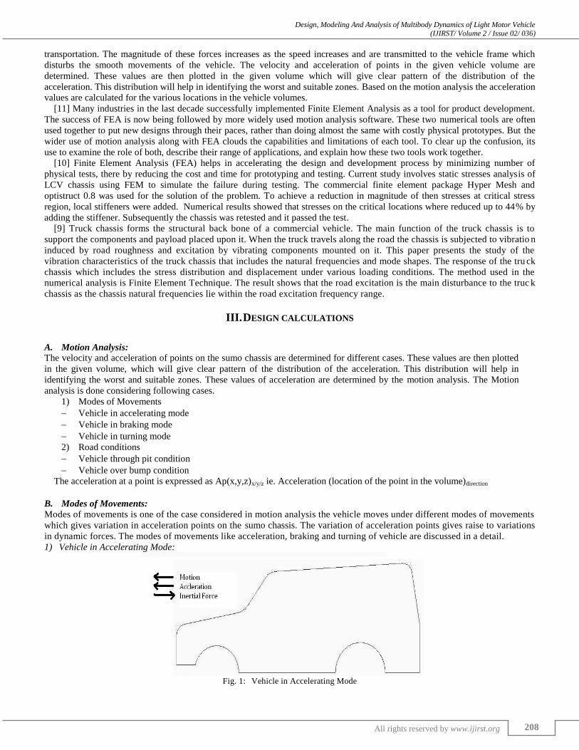
b) Vehicle in Turning Mode:
The vehicle is moving on a curved track, the vehicle will experience an angular speed with respect to the radius of curve about
vertical y axis.
c =
where, Vv = Linear velocity of vehicle = 30 km/hr = 8.33 m/s
Rc = Radius of curve of turn = 1500 mm
c =
c = 5.553 rad/s
Assuming that the vehicle is having a uniform speed while turning. This acceleration of the points on the sumo chassis will be
in xz plane i.e, in the z direction. The centrifugal acceleration will be
At p(x,y,z) = c2 * Rp
Where, At is the acceleration of a point expressed in the coordinate system and Rp is the radial distance of point from the
center of turn „I‟ of the y axis in fig.1 Rt is expressed in terms of the radius of turn
Road Condition F.
a) Vehicle through Pit Condition:
The angular velocity for rotation about left track:
p p(x,y,z)x = Z
zyxpV xyp ),,(
p p(x,y,z)x =
p p(x,y,z)x = 5.88 rad/s
The angular velocity for rotation about rear axle of the sumo chassis:
p p(x,y,z)z = X
zyxpV xyp ),,(

Design, Modeling And Analysis of Multibody Dynamics of Light Motor Vehicle (IJIRST/ Volume 2 / Issue 02/ 036)
All rights reserved by www.ijirst.org 214
p p(x,y,z)z =
p p(x,y,z)z = 20 rad/s
The resultant of the above two rotations for rotation about diagonally opposite corner:
p p(x,y,z)xz = XZ
zyxpV xyp ),,(
p p(x,y,z)xz =
p p(x,y,z)xz = 23.52 rad/s
The acceleration due to these angular velocities about left track:
Ap p(x,y,z)xy = 2
p p(x,y,z)x * z
Ap p(x,y,z)xy = 5.882 * 0.85
Ap p(x,y,z)xy = 29.38 m/s2
The acceleration due to these angular velocities about rear axle:
Ap p(x,y,z)xy = 2
p p(x,y,z)z * x
Ap p(x,y,z)xy = 202 * 0.25
Ap p(x,y,z)xy = 100 m/s2
The result of these two acceleration:
Ap p(x,y,z)xy = 2
p p(x,y,z)xz.xz
Ap p(x,y,z)xy = 23.522 * 0.25*0.85
Ap p(x,y,z)xy = 117.55 m/s2
Sin φ =
=
Φ = sin-1
,
Φ = 56.830
Considering the Different Speed of the Vehicle:
For 30km/hr (8.33m/s);
The velocity in downward direction is calculated using the following relation:
Vp p(x,y,z)xy = )2/(cos2 2
vV
Vp p(x,y,z)xy =
Vp p(x,y,z)xy = 5.38 m/s
For 40km/hr (11.11m/s);
Vp p(x,y,z)xy = 7.18 m/s
For 50km/hr (13.88m/s);
Vp p(x,y,z)xy = 8.97 m/s
For 80 km/hr (22.22 m/s);
Vp p(x,y,z)xy = 14.36 m/s
For 100 km/hr (27.77 m/s);
Vp p(x,y,z)xy = 17.94 m/s
For 120 km/hr (33.33 m/s);
Vp p(x,y,z)xy = 21.54 m/s
b) Vehicle over Bump Condition:
Considering the different speed of the vehicle the velocity in y direction is calculated using the following relation :

Design, Modeling And Analysis of Multibody Dynamics of Light Motor Vehicle (IJIRST/ Volume 2 / Issue 02/ 036)
All rights reserved by www.ijirst.org 215
For 30 km/hr (8.33m/s);
VBP P(x.y.z) = 22)5.0(
5.0
hw
wVv
VBP P(x.y.z) =
√
VBP P(x.y.z) = 3.36 m/s
For 40 km/hr (11.11m/s);
VBP P(x.y.z) = 4.48 m/s
For 50 km/hr (13.88 m/s);
VBP P(x.y.z) = 5.60 m/s
For 80 km/hr (22.22 m/s);
VBP P(x.y.z) = 8.97 m/s
For 100 km/hr (27.77 m/s);
VBP P(x.y.z) = 11.21 m/s
For 120 km/hr (33.33 m/s);
VBP P(x.y.z) = 13.46 m/s
c) Dynamic Forces:
For 30 km/hr (8.33 m/s);
F = l
EmaSA2
Where E = Elasticity = 2X10⁵ N/mm
2
m = Mass of link = 50 Kg
a = Acceleration = Velocity / Time;
t = 4 sec(assume)
S = Clearance = 190 mm
A = Area (From Table No. 5.1(a))
l = Length (From Table No. 5.1(a))
F = √
F = 22524.89 N
For 40 km/hr (11.11 m/s);
F = 26009.5 N
For 50 km/hr (13.88 m/s);
F = 29079.51 N
For 80 km/hr (22.22 m/s);
F = 36783.03 N
For 100 km/hr (27.77 m/s);
F = 41124.64 N
For 120 km/hr (33.33 m/s);
F = 45049.79 N
The table shows the details of each component of sumo chassis.
Table – 1
Details of each component

Design, Modeling And Analysis of Multibody Dynamics of Light Motor Vehicle (IJIRST/ Volume 2 / Issue 02/ 036)
All rights reserved by www.ijirst.org 216
IV. ANALYSIS
Cad Model of Tata Sumo: A.
Front View: 1)
Fig. 6: Front view
Top View: 2)
Fig. 7: Top view
Side View: 3)
Fig. 8: Side view
Drafting & Detailing: 4)
Fig. 9: Drafting & Detailing
Material Properties: B.
In this project, we use two types of material are as:
Aluminum Alloy (7079-T6):
Density = 2770 kg/m3
Youngs Modulus = 7.2E+10 Pa
Poission Ratio = 0.33

Design, Modeling And Analysis of Multibody Dynamics of Light Motor Vehicle (IJIRST/ Volume 2 / Issue 02/ 036)
All rights reserved by www.ijirst.org 217
Tensile Yield Strength = 5.03E+08 Pa
Compressive Yield Strength = 5.03E+08 Pa
Tensile Ultimate Strength = 5.72E+08 Pa
Compressive Ultimate Strength = 0 Pa
Meshing: 1)
ANSYS meshing technologies provide physics preferences that help to automate the meshing process. For an initial design, a
mesh can often be generated in batch with an initial solution run to locate regions of interest. Further refinement can then be
made to the mesh to improve the accuracy of the solution. There are physics preferences for structural, fluid, explicit and
electromagnetic simulations. By setting physics preferences, the software adapts to more logical defaults in the meshing process
for better solution accuracy.
Other physics-based features that help with structural analysis include:
Automated beam and shell meshing
Editable contact definitions
CAD instance modeling/meshing
Rigid-body contact meshing
Solver-based refinement
Thin solid-shell meshing
After Meshing in ANSYS Software, find out Nodes and Element
Nodes: 18208
Element: 17676
Fig. 10: Meshing
Boundary Condition: C.
Force: 1)
Fig. 11: Fixed Support
Frictionless Support: 2)
Fig. 12: Frictionless Support
Design, Modeling And Analysis of Multibody Dynamics of Light Motor Vehicle (IJIRST/ Volume 2 / Issue 02/ 036)
All rights reserved by www.ijirst.org 218
Above figure shows the boundary condition of sumo in ANSYS software and further process i.e, von-Mises stress, max. shear
stress and shear stress results are explained in next chapter.
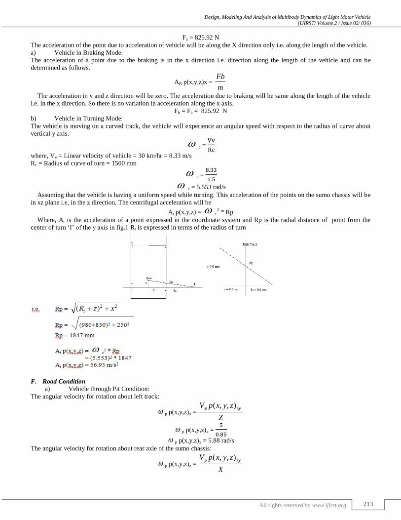
V. RESULT AND DISCUSSION
In this project, we work on different speed variations with constant material – Aluminum Alloy (7079-T6) are analyzed using
FEM ANSYS software following are FEM Analysis results:
30 Km/hr: A.
Von-Mises Stress 1)
Max.= 7906.7 Mpa
Fig. 13: Result of von-Mises Stress
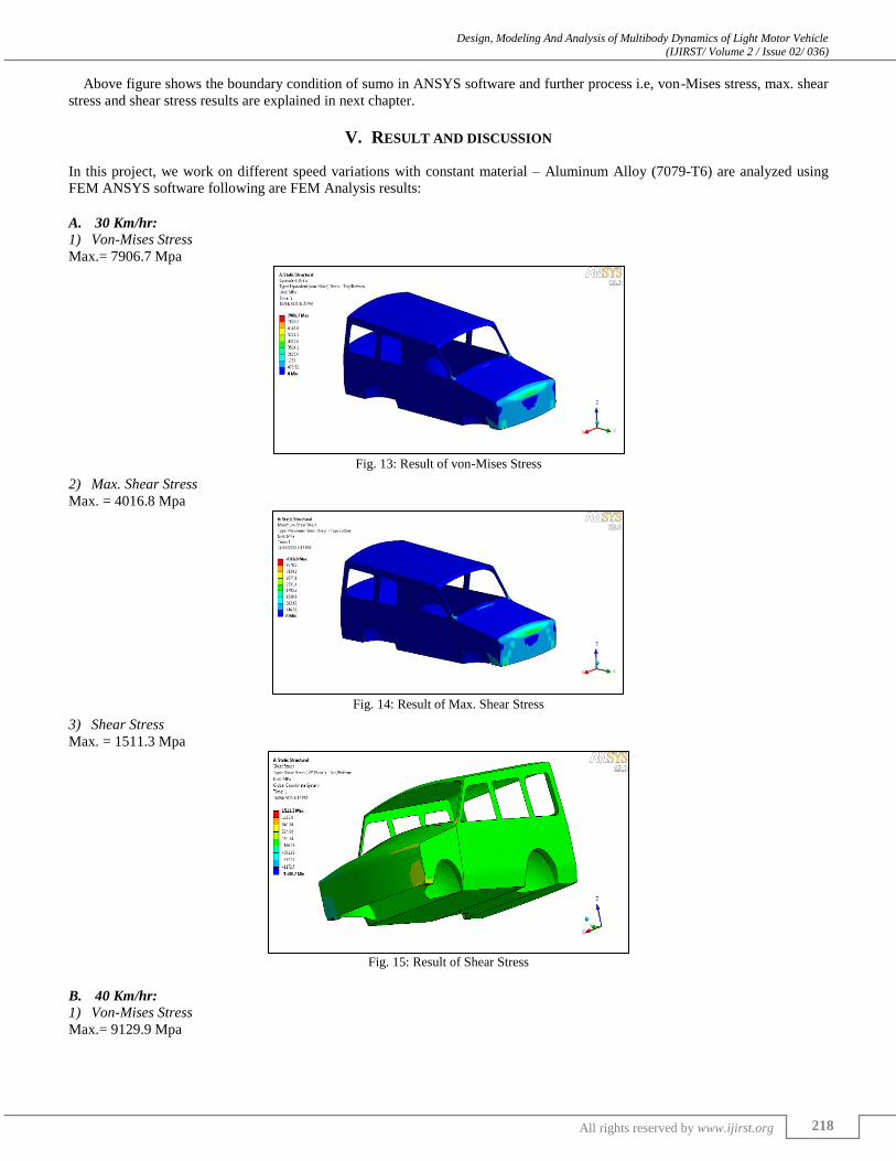
Max. Shear Stress 2)
Max. = 4016.8 Mpa
Fig. 14: Result of Max. Shear Stress
Shear Stress 3)
Max. = 1511.3 Mpa
Fig. 15: Result of Shear Stress
40 Km/hr: B.
Von-Mises Stress 1)
Max.= 9129.9 Mpa
Design, Modeling And Analysis of Multibody Dynamics of Light Motor Vehicle (IJIRST/ Volume 2 / Issue 02/ 036)
All rights reserved by www.ijirst.org 219
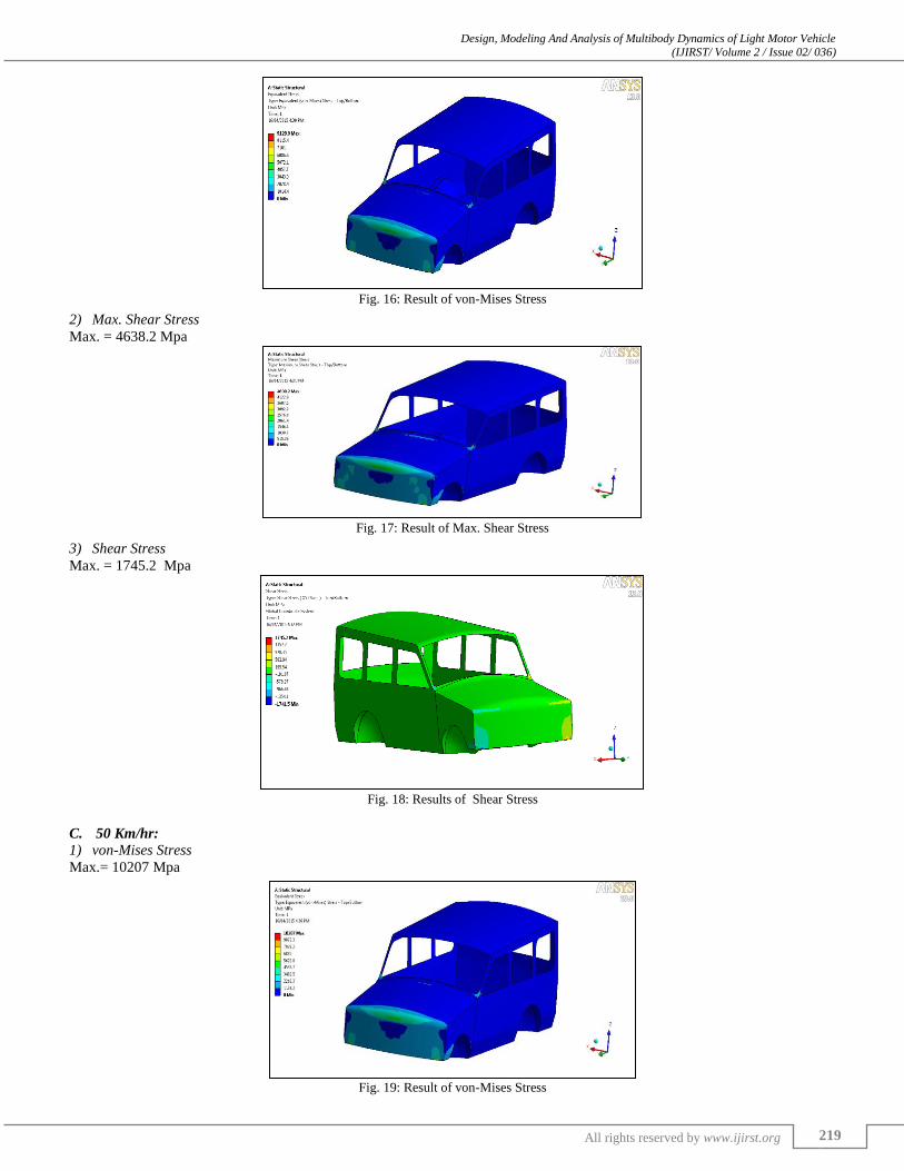
Fig. 16: Result of von-Mises Stress
Max. Shear Stress 2)
Max. = 4638.2 Mpa
Fig. 17: Result of Max. Shear Stress
Shear Stress 3)
Max. = 1745.2 Mpa
Fig. 18: Results of Shear Stress
50 Km/hr: C.
von-Mises Stress 1)
Max.= 10207 Mpa
Fig. 19: Result of von-Mises Stress

Design, Modeling And Analysis of Multibody Dynamics of Light Motor Vehicle (IJIRST/ Volume 2 / Issue 02/ 036)
All rights reserved by www.ijirst.org 220
Max. Shear Stress 2)
Max. = 5185.7 Mpa
Fig. 20: Result of Max. Shear Stress
Shear Stress 3)
Max. = 1951.1 Mpa
Fig. 21: Result of Shear Stress
80 Km/hr: D.
von-Mises Stress 1)
Max.= 12912 Mpa
Fig. 22: Result of von-Mises Stress
Max. Shear Stress 2)
Max 6559.5 Mpa
Fig. 23: Result of Max. Shear Stress

Design, Modeling And Analysis of Multibody Dynamics of Light Motor Vehicle (IJIRST/ Volume 2 / Issue 02/ 036)
All rights reserved by www.ijirst.org 221
Shear Stress 3)
Max. = 2468 Mpa
Fig. 24: Result of Shear Stress
100 Km/hr : E.
von-Mises Stress 1)
Max.= 14436 Mpa
Fig. 25: Result of von-Mises Stress
Max. Shear Stress 2)
Max. = 7333.7 Mpa
Fig. 26: Result of Max. Shear Stress
Shear Stress 3)
Max. = 2759.3 Mpa
Fig. 27: Result of Shear Stress

Design, Modeling And Analysis of Multibody Dynamics of Light Motor Vehicle (IJIRST/ Volume 2 / Issue 02/ 036)
All rights reserved by www.ijirst.org 222
120 Km/hr : F.
von-Mises Stress 1)
Max.= 15813 Mpa
Fig. 28: Result of von-Mises Stress
Max. Shear Stress 2)
Max. = 8033.7 Mpa
Fig. 29: Result of Max. Shear Stress
Shear Stress 3)
Max. = 3022.7 Mpa
Fig. 30: Result of Shear Stress
Analysis results clearly shows that the stresses for 30 Km/hr speed are lower than the other velocities and it is also shows in
tabular form : Table - 3
Results Comparision
SPEED 30 Km/hr 40 Km/hr 50 Km/hr 80 Km/hr 100 Km/hr 120 Km/hr
Mpa Mpa Mpa Mpa Mpa Mpa
STRESS
von-Mises Stress 7906.7 9129.9 10207 12912 14436 15813
Max. Shear Stress 4016.8 4638.2 5185.7 6559.5 7333.7 8033.7
Shear Stress 1511.3 1745.2 1951.1 2468 2759.3 3022.7

Design, Modeling And Analysis of Multibody Dynamics of Light Motor Vehicle (IJIRST/ Volume 2 / Issue 02/ 036)
All rights reserved by www.ijirst.org 223
VI. CONCLUSION
In this project, we concluded that the increase in stress values accordingly increasing speed. The speed 30 Km/hr will generate
low stress as compared with other velocities. The behavior of front portion of the vehicle are very important parameters in stress
distribution near front of the vehicle. This application are related experiments will be the subject of further investigations.
REFERENCES
[1] F.Oijer, “FE-based Vehicle Analysis of Heavy Trucks, Part II: Prediction of Force Histories for Fatigue Life Analysis”, Volvo Truck Corporation, S-405 08
Goteborg, Sweden.
[2] M.F.J. Luijten, “Lateral Dynamic Behaviour of Articulated Commercial Vehicles”, Eindhoven University of Technology, August 2010. [3] N.M.Shah, “Design and Analysis of Earth Mover – Wheel Loader Vehicle”,California State University, fall 2010
[4] Matthew C. Snare,“Dynamics model for predicting maximum and typical acceleration rates of passenger vehicles”, Virginia Polytechnic Institute and State
University, August 26, 2002. [5] R. Chakravaty, M.Tech. Project, Dynamic Forces Due to Heavy Linkages Mounted on Vehicle in Motion, VNIT Nagpur.
[6] www.technetalliance.com/uploads/tx_caeworld/DesCommVehChassBodyPart1990
[7] www.dot.state.mn.us/design/rdm/english/3e.pdf Road design manual Dec-2004.
[8] R.S. Khurmi & J.K. Gupta “Theory of Machine”,S chand & company LTD, New Delhi,1976, p.p.226-229.
[9] Teo Han Fui, Roslan Abd. Rehman, Static & Dynamic Structural Analysis of a 4.5 Ton Truck Chassis Dec-2007, No.24,56-57.
[10] S.S.Sane, Ghanashyam Jadhav And Anandaraj.H, Stress Analysis of Light Commercial Vehicle Chassis By Fem. [11] Paul Dvorak, Paul Kurowski, a closer look at motion analysis Jul-7-2005, London Ontario, Canada.
[12] Johansson and N.Gustavsson, FE-Based vehicle analysis of heavy trucks part- I: methods and models, department of vehicle dynamics and CAE, Volvo
truck corporation, S-40508 Goteborg, Sweden.