Embed Size (px)
Citation preview

Design and Metrology of a Precision XY
Planar Stage
by
Jeffrey Michael Gorniak
A thesis
presented to the University of Waterloo
in fulfillment of the
thesis requirement for the degree of
Master of Applied Science
in
Mechanical Engineering
Waterloo, Ontario, Canada, 2010
©Jeffrey Michael Gorniak 2010

ii
AUTHOR'S DECLARATION
I hereby declare that I am the sole author of this thesis. This is a true copy of the thesis, including
any required final revisions, as accepted by my examiners.
I understand that my thesis may be made electronically available to the public.
Jeffrey Michael Gorniak

iii
Abstract
In recent years, the manufacturing industry has seen an increase in demand for micro-components
in biomedical, opto-mechatronics, and automotive applications. Traditional machine tools are no
longer a viable solution to meet the tolerances required by the customers. Hence, new ultra-precision
machine tools have emerged with nanometer level accuracy in response to these demands. This thesis
presents a novel ultra-precision machine tool with the intent to bridge the gap between traditional
machine tools with larger work volumes and lower accuracy, and ultra-precision machine tools with
high accuracy and small work volumes. The machine was designed using a T-type gantry and
worktable configuration with a precision ground granite base, to achieve a work area of 300x300
mm2, with a maximum velocity of 1 m/s and a maximum acceleration of 10 m/s
2. Actuation is
provided by direct drive linear motors with high resolution feedback supplied by 4 µm grating linear
encoders with 4096x interpolation. Aerostatic porous bearings are employed to reduce the effect of
friction while maintain high stiffness of the guideways and structure. A Vacuum Pre-Loaded (VPL)
air bearing supports the worktable on the granite, decoupling vertical load from the gantry. Thermal
error reduction is achieved using environmental temperature control (20 ± 0.2°C) to help reduce
thermal errors. As well, internally cooled couplings were designed to remove heat generated by the
motors, thus further reducing the effects that contribute to thermal error.
The target static stiffness of the machine was 50 N/µm and was measured to be 22.2 N/µm and
23.9 N/µm in the x and y axes respectively. Frequency response experiments were used to identify the
open-loop transfer functions for each axis. A multivariable framework was implemented for the y-
axis due to the cross coupling between the primary and secondary motors of the gantry. Two
prominent vibration modes were identified at 68 Hz and 344 Hz. The first mode is attributed to the
rigid body yaw mode of the gantry while the higher frequency is related to the bending mode of the
beam. The first mode of the x-axis is seen at 220 Hz. A state space, active mode compensation control
law was developed for the y-axis, in collaboration with Mr. Daniel Gordon, which eliminates the
effects of the 68 Hz mode, allowing for high performance from the motors. The following error
during a high speed (200 mm/s) test was measured at 2.74 µm and 2.41 µm in the x and y axes
respectively.
Metrology tests using laser interferometry were performed in accordance with international and
American metrology standards for linear positioning, vertical and horizontal straightness, and yaw
and pitch errors. The results will be used for geometric error compensation in future work. Finally, an
overall error budget is presented with focus on the geometric, dynamic, servo, and thermal errors,

iv
where the maximum static resultant error of the machine was estimated to be 1.44 µm, and the
maximum dynamic resultant error of 3.69 µm.

v
Acknowledgements
This research is supported by the Canadian Foundation of Innovation (CFI), AUTO21, and the
Ontario Ministry of Research and Innovation granting agencies in Canada. Industrial contributions
were provided by New Way Precision, Heidenhain, ETEL, and Rock of Ages.
A special thanks to the machinists who provided quality products, valuable manufacturing
lessons, and guidance in the design of the machine. I would specifically like to mention the help of
Mr. J. Benninger and Mr. R. Wagner who not only assisted in every way possible, but were always
there to provide valuable insight to the machine’s design, as well as a good laugh. Thank you for all
your help gentlemen.
D. Gordon contributed to Chapter 4 with material from his Masters research in mode
compensating controller design.
I owe a lot of gratitude to Dr. Alkan Donmez, Dr. Shawn Moylan as well as many others at the
National Institute of Standards and Technology (NIST) for Chapter 5. Thank you for all your help in
machine tool metrology.
Thank you to Prof. F. Ismail and Prof. S. Lambert for reading this thesis and providing valuable
feedback.
And finally, I would like to thank my supervisor, Prof. K. Erkorkmaz. His devotion to research
and the success of his students is seen is everything he does. There are few words that can fully
express my gratitude for his guidance and the experience he has provided over these past years.
Thank you.

vi
Dedication
To my parents and Elisa.
†

vii
Table of Contents
AUTHOR'S DECLARATION ............................................................................................................... ii
Abstract ................................................................................................................................................. iii
Acknowledgements ................................................................................................................................ v
Dedication ............................................................................................................................................. vi
Table of Contents ................................................................................................................................. vii
List of Figures ....................................................................................................................................... ix
List of Tables ........................................................................................................................................ xii
Chapter 1 Introduction ............................................................................................................................ 1
Chapter 2 Literature Review .................................................................................................................. 5
2.1 Introduction .................................................................................................................................. 5
2.2 Precision Machine Design ............................................................................................................ 5
2.3 Machine Tool Metrology ............................................................................................................ 10
2.4 Conclusions ................................................................................................................................ 15
Chapter 3 Mechanical Design of the Precision Stage ........................................................................... 16
3.1 Introduction ................................................................................................................................ 16
3.2 Proposed Conceptual Design and Specifications ....................................................................... 16
3.3 Detailed Y-Axis (Gantry) and X-Axis (Table) Design .............................................................. 19
3.4 Dynamic Analysis ...................................................................................................................... 27
3.5 Static Stiffness Analysis ............................................................................................................. 31
3.6 Thermal Analysis ....................................................................................................................... 37
3.7 Error Budget ............................................................................................................................... 42
3.7.1 Linear Positional Error ........................................................................................................ 42
3.7.2 Straightness Error ................................................................................................................ 43
3.7.3 Angular Error....................................................................................................................... 43
3.7.4 Dynamic Error ..................................................................................................................... 44
3.7.5 Servo Error .......................................................................................................................... 45
3.7.6 Thermal Error ...................................................................................................................... 46
3.7.7 Overall Error Budget ........................................................................................................... 46
3.8 Conclusion .................................................................................................................................. 48
Chapter 4 Statics, Dynamics and Controls ........................................................................................... 49
4.1 Introduction ................................................................................................................................ 49
4.2 Static Stiffness ............................................................................................................................ 49

viii
4.3 Frequency Response Measurement and Identification ............................................................... 51
4.3.1 X-axis .................................................................................................................................. 51
4.3.2 Y-Axis ................................................................................................................................. 52
4.4 Controller Design ....................................................................................................................... 54
4.4.1 Parameter Identification ...................................................................................................... 54
4.4.2 X-Axis ................................................................................................................................. 57
4.4.3 Y-Axis ................................................................................................................................. 59
4.5 Conclusions ................................................................................................................................ 64
Chapter 5 Metrology ............................................................................................................................ 66
5.1 Introduction ................................................................................................................................ 66
5.2 Experimental Setup .................................................................................................................... 66
5.2.1 Linear Positioning Error Setup ............................................................................................ 66
5.2.2 Straightness Error Setup ...................................................................................................... 67
5.2.3 Angular Error Setup ............................................................................................................ 68
5.3 Abbe Error .................................................................................................................................. 68
5.4 Linear Positional Error ............................................................................................................... 70
5.4.1 X Linear Positioning Error (EXX) ...................................................................................... 70
5.4.2 Y Linear Positioning Error (EYY) ...................................................................................... 72
5.5 Straightness Error (EYX, EZX, EXY, EZY).............................................................................. 74
5.5.1 X Horizontal Straightness Error (EYX) .............................................................................. 74
5.5.2 X Vertical Straightness Error (EZX) ................................................................................... 76
5.5.3 Y Horizontal Straightness Error (EXY) .............................................................................. 78
5.5.4 Y Vertical Straightness Error (EZY) ................................................................................... 80
5.6 Angular Error (EBX, ECX, EAY, ECY) .................................................................................... 82
5.6.1 X Pitch Error (EBX) ............................................................................................................ 82
5.6.2 X Yaw Error (ECX) ............................................................................................................. 84
5.6.3 Y Pitch Error (EAY) ............................................................................................................ 86
5.6.4 Y Yaw Error (ECY) ............................................................................................................. 88
5.7 Conclusion .................................................................................................................................. 90
Chapter 6 Conclusions and Future Work ............................................................................................. 91
References ............................................................................................................................................ 94

ix
List of Figures
Figure 1-1. Conceptual design of the precision stage ............................................................................. 3
Figure 2-1. Axtrusion machine schematic [21] ...................................................................................... 7
Figure 2-2. Precision XY Stage with nanometer positioning [2] ........................................................... 8
Figure 2-3. Example of T-type CMM machine [22] .............................................................................. 9
Figure 2-4. XY stage designed to minimize Abbe error [23] ............................................................... 10
Figure 2-5. Error Definitions [24] ........................................................................................................ 11
Figure 2-6. Linear positioning error setup using a laser interferometer ............................................... 12
Figure 2-7. Straightness error setup using a laser interferometer ......................................................... 13
Figure 2-8. Angular error setup using a laser interferometer ............................................................... 13
Figure 2-9. Diagonal test for squareness of a planar stage ................................................................... 14
Figure 3-1. Conceptual design of stage (Top View). ........................................................................... 17
Figure 3-2. Conceptual design of precision stage. ................................................................................ 18
Figure 3-3. Three piece bearing support structure. ............................................................................... 19
Figure 3-4. Air bearing support and adjustment design, as well as the bearing housing with
1mm gap for injection of cement after adjustment of fly heights. .................................................. 20
Figure 3-5. Cement coverage for (a) single injection point located at the center and (b) two
injection points. ............................................................................................................................... 20
Figure 3-6. Injection channels for application of micro-shrink cement ............................................... 21
Figure 3-7. Y-axis cooling coupling shown in (a) collapsed view, (b) exploded view
highlighting internal cooling channels. ........................................................................................... 22
Figure 3-8. Air bearing lift-load curve showing non-linear stiffness [30] ........................................... 23
Figure 3-9. Encoder head and mounting bracket design for high stiffness .......................................... 24
Figure 3-10. Table design arrangement for minimal moment loads and measurement errors. ............ 24
Figure 3-11. (a) Underside of VPL showing different pressure regions, (b) Top view of
mounting datum ring. ...................................................................................................................... 25
Figure 3-12. VPL mounting plate showing minimum cement coverage, datum surface and O-
ring groove. ..................................................................................................................................... 26
Figure 3-13. Top plate of worktable with (a) bolt pattern and alignment pins, (b) with
trunnion installed. ............................................................................................................................ 26
Figure 3-14. Assembled prototype of precision XY stage. .................................................................. 27
Figure 3-15. Example of trajectory profile ........................................................................................... 28
Figure 3-16. Relationship between the 4 preloaded air bearings and a torsional spring. (a)
overall machine diagram and (b) geometrical relationship ............................................................. 29

x
Figure 3-17. Stiffness diagram of the machine to analytically determine the overall stiffness
in the x and y directions. ................................................................................................................. 32
Figure 3-18. Static bending diagram of the gantry beam. .................................................................... 32
Figure 3-19. Block diagram of a first order system with a PID controller ........................................... 34
Figure 3-20. Disturbance transfer function of a PID controller for a 1st order model system. ............ 35
Figure 3-21. Free body diagram of gantry pitch motion during constant acceleration ........................ 35
Figure 3-22. Lift-load curve for 80mm diameter air bearings [30] ...................................................... 36
Figure 3-23. Laboratory temperature with mean and standard deviation bounds ................................ 39
Figure 3-24. Y-axis coupling design .................................................................................................... 40
Figure 3-25. X-axis coupling design .................................................................................................... 41
Figure 3-26. Thermal analysis of y-axis coupling ................................................................................ 41
Figure 3-27. Thermal analysis of x-axis coupling ................................................................................ 42
Figure 3-28. Point of interest for (a) yaw, (b) roll and pitch axes of rotation. ..................................... 44
Figure 3-29. Simulated servo error ....................................................................................................... 45
Figure 4-1. X-axis stiffness grid pattern and results ............................................................................. 50
Figure 4-2. Y-axis stiffness grid pattern and results ............................................................................. 50
Figure 4-3. X-axis FRF ........................................................................................................................ 52
Figure 4-4. Y-axis direct and cross FRF’s ............................................................................................ 53
Figure 4-5. Y-axis FRF dependence on worktable position. (a) 2 – 3000 Hz, (b) 150 – 800 Hz ......... 54
Figure 4-6. X-axis FRF with identified model ..................................................................................... 55
Figure 4-7. Y-axis direct and cross FRF's and models ......................................................................... 57
Figure 4-8. X-axis (a) Nyquist and (b) Sensitivity plots ...................................................................... 58
Figure 4-9. X-axis (a) low speed and (b) high speed tracking results .................................................. 59
Figure 4-10. X-axis positioning accuracy ............................................................................................ 59
Figure 4-11. Y-axis controller state feedback design ........................................................................... 60
Figure 4-12. Y-axis open loop acceleration FRF’s............................................................................... 61
Figure 4-13. Y-axis sensitivity plot ...................................................................................................... 62
Figure 4-14. Contribution of active vibration damping on y-axis control ............................................ 63
Figure 4-15. Y-axis (a) low speed and (b) high speed tracking results ................................................ 63
Figure 4-16. Y-axis positioning accuracy ............................................................................................ 64
Figure 5-1. Linear positioning error setup ............................................................................................ 67
Figure 5-2. Straightness error setup ...................................................................................................... 67
Figure 5-3. Angular error setup ............................................................................................................ 68
Figure 5-4. Linear positioning error of the X axis ................................................................................ 70

xi
Figure 5-5. Grid view of X axis linear positioning error ...................................................................... 71
Figure 5-6. Linear positioning error of the Y axis ................................................................................ 72
Figure 5-7. Grid view of Y axis linear positioning error ...................................................................... 73
Figure 5-8. Horizontal straightness error of the X axis ........................................................................ 74
Figure 5-9. Grid view of X axis horizontal straightness error .............................................................. 75
Figure 5-10. Vertical straightness error of the X axis .......................................................................... 76
Figure 5-11. Grid view of X axis vertical straightness error ................................................................ 77
Figure 5-12. Horizontal straightness error of the Y axis ...................................................................... 78
Figure 5-13. Grid view of Y axis horizontal straightness error ............................................................ 79
Figure 5-14. Vertical straightness error of the Y axis .......................................................................... 80
Figure 5-15. Grid view of Y axis vertical straightness error ................................................................ 81
Figure 5-16. Pitch error of the X axis ................................................................................................... 82
Figure 5-17. Grid view of X axis pitch error ........................................................................................ 83
Figure 5-18. Yaw error of the X axis ................................................................................................... 84
Figure 5-19. Grid view of X yaw error ................................................................................................. 85
Figure 5-20. Pitch error of the Y axis ................................................................................................... 86
Figure 5-21. Grid view of Y pitch error ............................................................................................... 87
Figure 5-22. Yaw error of the Y axis ................................................................................................... 88
Figure 5-23. Grid view of Y yaw error ................................................................................................. 89

xii
List of Tables
Table 3-1. List of dynamic values of the machine. .............................................................................. 28
Table 3-2. List of required values to calculate the natural frequency of the yaw vibration of
the gantry. ........................................................................................................................................ 30
Table 3-3. List of terms required for calculating the first bending mode of the gantry beam. ............. 31
Table 3-4. Stiffness values of air bearings used on the machine. ......................................................... 31
Table 3-5. Gantry pitch parameter values ............................................................................................ 36
Table 3-6. Overall stiffness of the x and y axes for 3 different servo bandwidths. .............................. 37
Table 3-7. Areas of the stage which are sensitive to thermal changes. ................................................ 38
Table 3-8. Magnitude of error due to thermal changes. ....................................................................... 39
Table 3-9. Temperature data of laboratory. .......................................................................................... 39
Table 3-10. Predicted Error Budget. ..................................................................................................... 47
Table 5-1. Metrology results for the X linear positioning error (w.r.t. table top) ................................ 71
Table 5-2. Metrology results for the Y linear positioning error (w.r.t. granite surface) ....................... 73
Table 5-3. Metrology results for the X horizontal straightness error ................................................... 75
Table 5-4. Metrology results of the X vertical straightness error ......................................................... 77
Table 5-5. Metrology results for Y axis horizontal straightness .......................................................... 79
Table 5-6. Metrology results for Y axis vertical straightness ............................................................... 81
Table 5-7. Metrology results for the X pitch error ............................................................................... 83
Table 5-8. Metrology results for the X yaw error ................................................................................. 85
Table 5-9. Metrology results for the Y pitch error ............................................................................... 87
Table 5-10. Metrology results for the Y yaw error ............................................................................... 89
Table 5-11. Summary of accuracies from error measurements ............................................................ 90
Table 5-12. Summary of predicted accuracies assuming geometric error compensation .................... 90
Table 6-1. Final Error Budget .............................................................................................................. 93

1
Chapter 1
Introduction
The manufacturing industry has seen a growing demand for precision components in recent years.
Biomedical devices, automotive components and micro-optical moulds are some examples of these
precision manufactured components. Traditional milling practices have reached the limit of the
machines’ accuracy and cannot achieve the high tolerances now demanded in the micro-machining
field. In parallel with this limitation is the ability to machine complex three-dimensional surfaces of
micro components. These limitations coupled with the high demand from industry have created a
need for new multi-axis ultra-precision machine tools capable of creating complex geometry while
achieving the difficult tolerances required.
Typically, machine tools can achieve positioning accuracies on the order of tens of microns or
even microns. The new tolerances require positioning accuracies 100x more accurate, which is tens o
hundreds of nanometers. To achieve nanometer accuracy, machine designers need to identify the
sources of error and develop solutions to eradicate or minimize their effects. Previous research has
highlighted several key areas which yield the highest level of error for precision machines [1]. The
effect of thermal variation of the machine’s structure, as well as its environment, incorporates a large
amount of uncertainty in the position of the cutting tool relative to the workpiece. Thermal error alone
has the potential to yield parts which are beyond the specified tolerances for a micro-component. By
removing the heat generated from sources such as the cutting process, electric motors, friction, and
environmental changes, the repeatability of the machine will improve and positioning uncertainty
reduced.
Another source of error is the mechanical error of the guideways for a machine. The goal is to
move the tool in a specified motion without deviating from its desired path. However, all guideways
will contain some amount of error. There are several methods to minimize this error. One offline
method is to map all geometric errors within the work volume of the machine tool and record the
repeatable mechanical error [1]. Once the map is known, the toolpath can be shifted according to the
map to compensate for the error. A metrology frame is an example of an online compensation
technique, where positional deviations from the ideal location are measured in real-time. The
reference position is adjusted to compensate for the measured error, thus, applying active geometric
compensation [1].

Chapter 1 Introduction
2
To obtain a high dynamic response from the machine, the system must be designed for high
stiffness for several reasons. The first is to reduce the flexibility of the machine structure, which
causes positioning errors and is difficult to measure and compensate. The second is to shift vibration
resonances to a range of frequencies that will not be affected during normal operation of the machine.
It is a challenge to design a machine with high stiffness while keeping the mass and size of the
machine at an acceptable level. Precision machine design principles can be used to increase the
stiffness and improve the dynamics of the machine [1]. However, once the machine is built, it is
natural for vibrations to still occur. The drive system, with advanced control algorithms, can be used
to actively dampen the vibrations.
The objective of this research is to develop a novel 5-Axis ultra-precision machine tool for the
micro-machining industry to create products such as micro-optic moulds, impellers for continuous
flow heart pumps and Micro-Electrical-Mechanical-Systems (MEMS). However, due to the size of
the project, the scope of this thesis will focus on the design, metrology, and controller design for two
linear, orthogonal axes which comprise the planar stage of the machine. The proposed planar stage
will be the base of the machine to which the remaining linear and two rotary axes will be attached.
The machine is required to have a larger work area than most precision machines with greater
dynamic capabilities. However, its positioning accuracy should be on the same order as previous
precision machines, which were around 10 – 100 nm. Cutting loads during a micro machining process
are expected to be no more than 20 N, which should not induce errors greater than 0.4 µm. Therefore,
the target stiffness of the stage should be greater than 50 N/µm.
Chapter 3 discusses the design of the stage, as illustrated in Figure 1-1, which consists of a gantry
and worktable configuration commonly seen with Coordinate Measurement Machines (CMM) where
a linear guideway is present on one side of the gantry with a bridge extending over the work area
(300x300 mm2) of the machine.

Chapter 1 Introduction
3
Figure 1-1. Conceptual design of the precision stage
The bridge is orthogonal to the granite guideway and performs as a subsequent guideway for the
worktable. The weight of the worktable is traditionally supported by the gantry bridge, which leads to
deformation of the beam. This can cause positioning errors and decrease the stiffness of the machine.
Alternatively, a Vacuum Pre-Loaded (VPL) air bearing, commonly seen with photolithography
machines, is used to support the worktable on the granite base of the machine. The granite is precision
ground to accommodate the flatness of the VPL. The underside of the VPL consists of a
pneumatically pressurized region which lifts the worktable off the surface, while a vacuum region
preloads the bearing to the granite. This produces a stiff design which is resistant against vertical and
pitch loads. Another desired effect of the VPL is the negligible coefficient of friction between itself
and the granite. Aerostatic bearings are used to support the gantry on the granite base, and by
preloading the bearings, a high stiffness design with a negligible friction effect is achieved. To realize
high dynamic performance, direct drive linear motors are used to actuate the axes which will
accelerate the stage at 10 m/s2 to a maximum speed of 1 m/s. To reduce flexibility of the gantry and
actively compensate for structural vibrations, two motors are used to actuate the gantry located at
opposite ends of the beam.
Control laws are developed in Chapter 4 to position the stage with sub-micron to nanometer level
accuracy while also providing robust tracking performance during high transient motions. A
multivariable control law framework was used for the y-axis due to the cross coupling dynamics

Chapter 1 Introduction
4
between the two gantry motors. Identification of system parameters was completed by a Frequency
Response Function (FRF) measurements, which pass open loop sine wave inputs to the motors and
measures the relative magnitude and phase of the output from the encoders. These tests also helped to
identify the resonance frequencies and aided in advanced controller designs.
In Chapter 5, quasi-static metrology measurements are collected to map the geometric errors of
the stage. A laser interferometer was used to measure the linear positioning, vertical and horizontal
straightness as well as yaw and pitch rotational errors. The measured repeatable errors can be used to
improve the accuracy of the machine through geometric compensation.
Chapter 6 presents the conclusions of the thesis along with a final error budget and future work
for the project. Recommendations are listed for future design considerations.

5
Chapter 2
Literature Review
2.1 Introduction
This chapter presents a review of literature and industrial state-of-the-art in the areas of precision
machine design and machine tool metrology. Section 2.2 presents the principles of precision design
with its implementation on machine tools. Machine tool metrology using laser interferometry
techniques are defined and their principles of operation are explained in Section 2.3. Conclusions for
the chapter are presented in Section 2.4.
2.2 Precision Machine Design
Precision machine tools have become highly prominent in manufacturing practices to alleviate the
demand from industry for complex micro-components. Traditional machine tools have reached their
limit in terms of accuracy (1 µm). Hence, new machine tool designs were required to satisfy the new
fabrication tolerances. In response to this demand, researchers successfully developed ultra-precision
machines capable of nanometer level accuracy [2], [3], [4], [5]. Additionally, commercial designs of
precision machines were built, which offered a practical solution for achieving high accuracies [6],
[7], [8], [9]. A common denominator to all designs is the reduction of errors such as geometric,
thermal, and friction, while maintaining high stiffness of the structure.
Geometric error is comprised of error in the machine’s guideways, drive system such as ball-
screws and timing belts, and misalignment of components. This results in positional deviations of the
workpiece or tool tip, leading to errors during the machining process. These errors are often
predictable due to their mechanical nature and can be reduced by using proper compensation
techniques. A guideway for a machine tool is often precision ground or hand scraped, and is capable
of maintaining a straightness error less than one micron over a distance of 1 m. However, if
nanometer level accuracy is desired, compensation of geometric error can reduce the guideway error
to nanometer levels [1], [10]. Further explanation of geometric error compensation by laser
interferometry is explained in Section 2.3. Drive systems which include ball-screw drives, timing
belts, and mechanical bearings are prone to geometric errors. Lead error of ball-screws is periodic and
is dependent on the quality of the groove on the shaft. Compensation of the lead error was performed
by Kamalzadeh by comparing the rotational position of the drive motor and the linear displacement of

Chapter 2 Literature Review
6
the work table [11]. A sinusoidal error emerged with a period identical to that of the ball-screw. A
model-based compensation was used to predict the error and adjust the trajectory input accordingly.
However, future changes to the drive system setup would require a re-measurement of the lead error,
which can be time consuming and not practical. Ironless direct drive linear motors are a popular
alternative to actuating machine tools, due to their minimal cogging effect and absence of lead errors
[4], [12], [13]. They also provide a non-contact, high dynamic response over large travel ranges.
Shinno et al. used voice coil motors to actuate an X-Y Planar Motion Table System, which was
capable of positioning the table within one nanometer and providing high stiffness during cutting tests
[2]. However, voice coil motors have limited range of travel, only 10 mm for the motion system in
[2].
One of the largest sources of error for a precision machine is thermal error. Fluctuations or
gradients in temperature of a machine’s components cause materials to expand and contract, causing
positioning errors. Temperature throughout the machine is difficult to measure, since it can be
different at various locations, and is even more difficult to predict. Research studying the thermal
properties of machine tools has been widely studied [1], [14]. It was found that regulating the
temperature of the environment reduced changes in the machine’s temperature, thus increasing the
repeatability of the machine. The material to build the machines has also been analyzed. Materials
that have low or negligible coefficients of thermal expansion, such as Invar or Zerodur, expand less
under similar temperature conditions than regular engineering materials like steel or aluminum [15].
For example, a 1 m piece of steel will expand 12 µm for every 1°C increase of temperature. Invar will
expand only expand 1.3 µm in the same scenario. However, Zerodur and Invar are higher in cost and
are not practical for the average machine shop. Therefore, more emphasis is directed to controlling
the temperature of the environment and the machine. A major source of thermal energy is produced
by the electric components of the machine, such as the servo motors, and mechanical components, for
instance the ball-screw nut interface or roller bearings. Some servo motors are now supplied with the
option of liquid cooling channels which surround the motor and remove thermal energy [16]. The
heat generated by roller bearings is created from the friction of the rollers against the guideway or
raceway.
Friction is a difficult effect to predict and compensate, due to its non-linear nature. Its
compensation requires accurate modeling, which in servo control practice can be achieved using a
disturbance observer [2], [17]. Another disadvantage of friction is the creation of heat during motion,
causing the guideways to expand or warp leading to larger, less repeatable positional errors. It is
common practice for machine tool operators to perform a warming routine in order for the machine to
reach thermal equilibrium [1]. Aerostatic bearings are often used to reduce or even remove friction as

Chapter 2 Literature Review
7
shown in [3], [18]. A thin, pressurized film of air between the bearing and guideway create a nearly
frictionless (µ ~ 10-5
) contact, while maintaining high stiffness. Typical roller bearings have a friction
coefficient of µ ~ 10-3
. In parallel with aerostatic bearings are hydrostatic bearings, which use a thin
film of oil between the bearing and guideway. They provide higher stiffness than aerostatic bearings;
however it can be difficult to control the oil flow and leaks. Aerostatic bearings are much cleaner,
environmentally friendly and economical. They are commonly used in CMM and photolithography
machines, since they are ideal for clean room and high accuracy applications. A disadvantage to
aerostatic bearings is their unidirectional stiffness. To achieve bidirectional stiffness, a preloaded air
bearing arrangement is used. Recently, a new type of aerostatic bearing was designed, which uses
vacuum pressure between the bearing and the guideway along with the pressurized air to create two
counteracting forces. Such bearings are called Vacuum Pre-Loaded (VPL) bearings and have high
bidirectional stiffness properties [19]. As well, the air gap between the bearing and guideway can be
controlled by adjusting the two pressures. VPL technology was used by Shinno to provide a vertical
stiffness of the machine of 84 N/µm [20]. VPL technology is also seen in photolithography machines
to support and accurately position 300 mm Silicon wafers.
Cortesi developed a single axis drive system with many of the principles mentioned above [21].
The Axtrusion machine, as seen in Figure 2-1, uses a precision ground granite base, aerostatic
bearings, and a direct drive linear motor. The machine has a range of 320 mm.
Figure 2-1. Axtrusion machine schematic [21]

Chapter 2 Literature Review
8
The linear motor has a dual purpose as it provides linear positional actuation, as well as a
preloading force for the air bearings. The motor is angled such that the vertical and horizontal force it
applies preloads the bearings to achieve the recommended fly height for the air bearings. The average
vertical stiffness was measured to be 422 N/µm.
Shinno developed an XY positioning table using an alumina ceramic base with 5 vacuum
preloaded aerostatic bearings, and 8 voice coil motors [2]. The schematic of this machine is shown in
Figure 2-2.
Figure 2-2. Precision XY Stage with nanometer positioning [2]
The machine has a work area of 20x20 mm2 with a maximum acceleration of 1.6 m/s
2. The
vertical stiffness is 191 N/µm and is capable of 1 nm positioning in both axes. Sub-nanometer
resolution is achieved by laser encoders and plane mirrors, that are located such that measurement
errors is negligible. The coils of the motors are located on the base to minimize thermal energy from
reaching the stage. The stage is in a non-contact environment, thus removing any non-linear effects.
Cutting tests of Tungsten Carbide (WC) at 1mm/s were performed with tracking errors during cutting
of 2 nm and 5 nm in the x and y axes, respectively. The remarkable results show the high accuracy
potential for ultra-precision machines.

Chapter 2 Literature Review
9
CMM machines are known for their sub-micron positioning capabilities. They are required to be
accurate and highly repeatable in order to verify tolerances of a component are within their
specification. An example of a CMM is shown in Figure 2-3.
Figure 2-3. Example of T-type CMM machine [22]
The CMM above has a T-type gantry design with a guideway on one end and the gantry beam
extending over the workspace. The beam of the gantry operates as a guideway for a second axis.
Actuation of the gantry is provided by one motor next to the guideway on the base.
A XY stage was developed by Heidenhain at the National Institute of Standards and Technology
(NIST), which consists of a XY grid encoder and voice coil motors. Figure 2-4 shows a picture of the
stage. The encoder head is located directly in line with the tool above the worktable (not shown in the
figure). The motors actuate near the center of mass of the stage, causing minimal moment loads. The
intention of the design is to minimize Abbe errors.

Chapter 2 Literature Review
10
Figure 2-4. XY stage designed to minimize Abbe error [23]
The stage has a work area of 50x50 mm2 and uses cross-roller bearings and rails as guideways.
The machine shows the potential for larger work areas while maintaining high positioning accuracies.
2.3 Machine Tool Metrology
Metrology of machines tools is common practice to measure the mechanical accuracy of a
machine. It provides the user with detailed information about the actual location and orientation of the
machine throughout its work volume. This information is highly valuable to both the machine tool
builders and customers for various reasons. The builder can provide the results of the measurements
to authenticate the accuracy of their machine and provide this to a customer as a confirmation of the
machine’s accuracy. The customer is able to compare different machines and review the metrology
results of each machine and use their engineering judgment when deciding which machine to use for
their application. Most customers look for an overall accuracy value called the volumetric error, as
explained in [24], for a machine as a simple yet effective way to compare each machine. However,
there are many measurements required to calculate this value. The international machine tool
metrology standard ISO-230-1 [24] along with ASME B5.54-2005 [25] are used for definitions,
terminology and analysis methods.
For each axis, there are six degrees of error; three linear and three rotational error motions. For
multi-axis machines, an additional error value is included, which is the angular deviation from the
desired orientation between each axis. For a two-axis planar stage, there exist 13 error motions: six
linear errors, six rotational errors, and one orientation error. The definition of each error is dependent
on the direction of travel and its relation to the machine’s coordinate frame. The linear errors are
defined as linear positioning displacement, horizontal straightness and vertical straightness. The

Chapter 2 Literature Review
11
rotational errors are defined as yaw, pitch and roll. Since a machine’s axes are typically setup to be
orthogonal to each other, the orientation error of axes is often called the squareness error. The
following figure outlines the error definitions for a single axis.
Figure 2-5. Error Definitions [24]
Where
EAX angular error motion around A-axis (Roll)
EBX angular error motion around B-axis (Yaw)
ECX angular error motion around C-axis (Pitch)
EXX linear positioning error motion of X-axis positioning deviations of X-axis
EYX straightness error motion in Y-axis direction
EZX straightness error motion in Z-axis direction
Laser interferometry is an accurate and reliable method for machine tool metrology and is used
for the measurements presented in Chapter 5. The laser interferometer uses a beam with a known
wavelength and the principles of wave interference to determine the desired error value. The signal is
interpolated to produce measurement resolutions less than one nanometer. A laser beam is emitted
from the laser head, which is then sent through a series of optical mirrors and reflectors. The signal is
returned to the laser head where the interference signal is detected. For linear displacement
measurements, the initial beam is sent through an interferometer where it is split. One beam is sent to
a stationary reference retro-reflector and the other is sent to a retro-reflector on the moving object.
The beams from the two reflectors return to the interferometer where they recombine, forming an
interference pattern and are sent back to the laser for counting the number of fringes. Figure 2-6
shows the setup.

Chapter 2 Literature Review
12
Figure 2-6. Linear positioning error setup using a laser interferometer
The medium in which the beam travels can shift the wavelength of the laser from its nominal
value. The nominal wavelength is accurately measured in a vacuum to eliminate environmental
effects. When measurements are performed on a machine, the environment has temperature, pressure
and humidity levels which slightly decrease the wavelength. Sensors are situated within the machine
and in close proximity to the laser, to measure the environment properties. Differences from the
nominal wavelength measurement conditions are collected and the actual wavelength is calculated
using the modified Edlén formula [26]. This process is called environmental compensation.
Compensation is only required for linear displacement tests and not for straightness or angular
measurements. During straightness and angular tests, the difference between the beam lengths is
measured. The influence of environmental changes is negligible compared to the measured value,
therefore it is not required.
The setup for straightness measurements requires optics designed specifically for this test. The
optics includes a straightness interferometer (Wollaston prism) and bi-mirror straightness reflector.
The beam is sent to the prism where it is split at an acute angle and both beams are sent to the
reflector. The reflector returns the beams to the prism where they are re-joined and sent back to the
laser head. The prism is located on the moving object while the reflector is stationary. Deviations of
the prism from the straight line path will alter the lengths of the two beams sent to the reflector. One
beam will increase in length while the other decreases. The change in lengths will result in a changing
interference pattern registered at the laser head. From this, the amount of straightness error can be
calculated. Two tests must be completed with the optics turned 90o between each test to collect all of
the straightness error. Figure 2-7 illustrates the straightness setup for one orientation.

Chapter 2 Literature Review
13
Figure 2-7. Straightness error setup using a laser interferometer
Laser interferometry cannot measure all angular errors. Roll cannot be measured, as its axis of
rotation is parallel to the direction of travel and the laser path is insensitive to this motion. Roll is
typically measured using a precision angular level and compared to a reference level. The setup for
yaw and pitch includes an angular interferometer and angular reflector. The beam is emitted from the
laser head to the interferometer, where it is split. One beam passes straight through while the other is
reflected orthogonal to the original beam. The second beam is sent to an angle mirror, which directs
the beam to be parallel with the first beam. Both beams are now parallel to the direction of travel.
They are sent to the reflector, which consists of two retro-reflectors. The beams are sent back to the
laser head along the same path. Rotation of the reflector will alter the lengths of the two beams. The
change in lengths will result in a different interference pattern read at the laser head. From this, the
amount of angular error can be calculated. Two tests must be completed with the optics turned 90°
between each test to collect all of the angular error data. Figure 2-8 illustrates the angular setup.
Figure 2-8. Angular error setup using a laser interferometer

Chapter 2 Literature Review
14
Squareness of two orthogonal axes can be measured using a laser by a couple of methods. The
first is using laser interferometry with specialized optics, however, the optics are expensive and were
not available to the author. A second method is to use the linear positioning setup and measure the
displacement along the two diagonals of the workspace. Figure 2-9 demonstrates the measurement
paths and the geometry characteristics for a setup with actual squareness.
Figure 2-9. Diagonal test for squareness of a planar stage
The squareness error is the value of 𝜃, which can be calculated by measuring the diagonals ℓ1 and
ℓ2. The two lengths can be calculated analytically with Equations (1.1) and (1.2).
ℓ12 = ℓ + 𝛿𝑥
2 + (ℓ − 𝛿𝑦)2 (1.1)
ℓ22 = ℓ − 𝛿𝑥
2 + (ℓ − 𝛿𝑦)2 (1.2)
Subtracting Equation (1.2) from (1.1) and solving for 𝛿𝑥 results in Equation (1.3).
𝛿𝑥 =
ℓ12 − ℓ2
2
4ℓ (1.3)
Expanding the numerator in Equation (1.3) and simplifying gives,
𝛿𝑥 =
(ℓ1 + ℓ2)
2
2ℓ
(ℓ1 − ℓ2)
2ℓ
𝛿𝑥 =(ℓ1 − ℓ2)
2
(1.4)
The squareness error is calculated using the arcsine of 𝛿𝑥/ℓ, shown in Equation (1.5).
𝜃 = 𝑠𝑖𝑛−1
𝛿𝑥
ℓ (1.5)
Substituting for 𝛿𝑥 , Equation (1.5) becomes,

Chapter 2 Literature Review
15
𝜃 = 𝑠𝑖𝑛−1
(ℓ1 − ℓ2)
2ℓ (1.6)
This method is further explained in the international standard ISO-230-6:2002 [27] as an
acceptable means of measuring squareness of machine tool axes.
2.4 Conclusions
This chapter has presented a survey of academic literature and industrial practice relevant to
precision machine tool design and metrology. The design of a precision machine uses precision
engineering principles to reduce the effect of errors on the positional accuracy of the machine.
Geometric, thermal and friction errors are designated as the largest contributors to the error on a
machine tool. Most geometric errors are repeatable in nature and can be predicted. Compensation of
these errors is common practice to improving the accuracy of a machine. Thermal errors remain as
one of the largest and most difficult sources to eradicate. Temperature fluctuations of the environment
and concentrated heat sources expand and contract the machine’s components, causing positional
deviations. Temperature controlled laboratories and cooling circuits help reduce warping of the
machine and lead to better accuracy. Errors due to friction tend to be non-linear in nature and can be
difficult to predict and compensate. Hydrostatic and aerostatic bearings and non-contact motors are
emerging as popular solutions to reduce and even eliminate friction errors, leading to better positional
accuracy.
Metrology covers the analysis of a machine tool’s accuracy, since it produces profiles of each
type of error, which can be measured accurately and applied in geometric error compensation. Laser
interferometry uses the wavelength of the beam and interpolation of wave interference to produce
resolutions of less than one nanometer. The subsequent Chapters utilize many of the design and
measurement techniques that were covered in this literature survey.

16
Chapter 3
Mechanical Design of the Precision Stage
3.1 Introduction
In this chapter, a novel design of an ultra-precision planar stage is presented. In Section 3.2, the
initial concept and prototype design is developed which highlights key areas and sizing of
components. The design is separated into two individual axes and is discussed in Section 3.3, which
focuses on the design of the Y-axis (gantry) and the X-axis (work table). Dynamic and static analyses
are presented in Sections 3.4 and 3.5 respectively. A thermal analysis of the machine is completed;
the effects of temperature fluctuations and gradients are discussed in Section 3.6. Finally, an error
budget of the stage is developed in Section 3.7, which outlines the major sources of error and possible
methods to reduce the error of the machine. The conclusions for the design are outlined in Section
3.8.
3.2 Proposed Conceptual Design and Specifications
The ultra-precision planar stage was designed with the intention of bridging the gap between
traditional machine tools, which have a large work area (1 – 2 m) and moderate level accuracy (1 – 10
µm), and nanometer (1 – 10 nm) accuracy machines with small work areas (< 20x20 mm2). Designing
a machine with a large work area and nanometer level accuracy opens up new opportunities in the
micro machining industry, to fabricate macro components with micro features using one machine and
one setup. The stage presented in this chapter has a work area of 300 mm x 300 mm with nanometer
position feedback and is capable of motion transients with high speed (1 m/s) and high acceleration (1
g). Figure 3-1 details the conceptual design of the machine.
The stage incorporates a T-type gantry and worktable configuration which is adapted from CMM
designs. The gantry provides motion in the y-axis while the worktable realizes motion in the x-axis
with respect to the gantry. The gantry is supported by porous carbon air bearings on a precision
ground granite base. Four round air bearings support the weight of the gantry while four preloaded
rectangular bearings provide alignment to the granite guideway. The worktable is supported by a 12”
x 12” (305 mm x 305 mm) Vacuum Pre-Loaded (VPL) air bearing, which utilizes both positive and
negative pressure to preload the table to the granite surface. The VPL increases the vertical and pitch
stiffness and transfers the load of the table and workpiece into the granite rather than the gantry beam.

Chapter 3 Mechanical Design of Precision Stage
17
Figure 3-1. Conceptual design of stage (Top View).
Four additional rectangular bearings provide support and alignment of the worktable along the
gantry beam. Actuation of the gantry is achieved by two direct drive linear motors. The primary
motor is located on the side closest to the granite guideway, while the secondary motor is located on
the opposite end to increase the stiffness of the beam and decrease undesired vibrations at the free
end. Actuation of the worktable is realized by one direct drive linear motor located on the top of the
gantry beam. High resolution position feedback (4 µm grating x4096 interpolation) is realized by
glass scale linear encoders located next to their associated motors.
Design objectives of the machine include a target stiffness of 50 N/µm, positioning repeatability
of < 1 µm and dynamic accuracy of 1-5 µm. This can be achieved by proper mechanical design of the
stage structure, robust controller design, and compensation of known errors. Errors due to thermal
deformation become more prevalent as the accuracy of a machine improves below one micron. This
is due to thermal expansion of materials, which is on the order of 0 – 30 ppm/°C. The effect of
thermal deformation of machine tools has been widely studied and has been noted as one of the most
difficult sources of error to combat [1]. Some methods to minimize thermal error are temperature
controlled environments, moving the machine slowly to prevent mechanical heat generated from
friction, liquid cooling critical areas of the machine, and using materials with low coefficients of
thermal expansion. Also, symmetrical designs and using materials with high thermal conductivity
(like aluminum) help alleviate thermal problems to a certain extent.
A second source of error is friction which is non-linear and difficult to model or predict. CNC
machine tools already incorporate friction compensation features, however they are typically simple
in nature (only considering constant bidirectional Coulomb friction) and do not properly model the
complexity of the actual friction. To model the friction profiles of guideways and drive systems, such
as ball-screws or roller bearings, is difficult and not conducive to time constraints. Air bearings

Chapter 3 Mechanical Design of Precision Stage
18
provide an alternative solution to mechanical guideways. Air bearings produce a pressurized film of
air between a flat reference surface and itself. The gap is called the fly height, which is suggested by
the manufacturer to be approximately 5 µm. The bearings operate on the squeeze film damping effect,
which results in higher dynamic stiffness as well as negligibly small friction coefficients (µ = 0.00001
[28]). The use of air bearings eliminates the need to model friction and compensate its error
contribution.
A mechanical drive system can also constitute sources of error through backlash and lead error,
such as in ball screw drives and gears. To compliment the frictionless bearings, direct drive linear
motors were selected to provide actuation to the stage. They are non-contact and are capable of high
acceleration and high speed.
The proposed stage design is presented in the Figure 3-2 which incorporates the above mentioned
features.
Figure 3-2. Conceptual design of precision stage.

Chapter 3 Mechanical Design of Precision Stage
19
3.3 Detailed Y-Axis (Gantry) and X-Axis (Table) Design
During the design of the gantry, special attention was focused on the four preloaded air bearings,
since their location provides the majority of the yaw and x-axis stiffness for the stage. To maximize
yaw stiffness, the bearings are positioned with the greatest distance apart while maintaining a travel
range of 300 mm for the y-axis. The bearing size is 150 mm x 75 mm and was selected for its high
stiffness (324 N/µm) and size. The structure supporting the bearings needs to be stiff in order to
decrease gantry splay and deformation as the bearings are preloaded. Each bearing is preloaded with
approximately 2500 N to achieve the recommended fly height of 5 µm. The structure around the
bearings was designed with three components. The first reason was to minimize the number of bolted
joints which reduce stiffness, and secondly to simplify the fabrication of the structure. Ideally the
structure would be made of one piece, however, features such as the pockets which house the
bearings would be very difficult to machine.
Figure 3-3. Three piece bearing support structure.
The bearings are mounted using ball mounting screws, which allow for self alignment of the
bearings to their guideway. However, the stiffness of the bearing can decrease as the spherical joint is
allowed to rotate. Therefore, micro-shrink cement [29] should be applied between the bearing and the
surrounding structure which eliminates rotational movement and increases stiffness. The structure is
designed with a 1 mm gap between the bearing and the structure, which is shown in the cross section
view of Figure 3-4.

Chapter 3 Mechanical Design of Precision Stage
20
Figure 3-4. Air bearing support and adjustment design, as well as the bearing housing with
1mm gap for injection of cement after adjustment of fly heights.
The cement is installed by injection from the backside of the bearings. Cortesi from the
Massachusetts Institute of Technology (MIT) also performed the same process with their Axtrusion
single-axis drive [21]. They noted that two injection points spaced out along the back surface of the
bearing provides better coverage than one located in the center. Therefore, two injection points were
incorporated into the design of the housing. To simplify the injection process, channels were routed to
the exterior of the gantry to provide ample room for syringes to inject the cement. Figure 3-6
illustrates the design of the channels in the structure and their location with reference to the bearings.
(a) (b)
Figure 3-5. Cement coverage for (a) single injection point located at the center and (b) two
injection points.

Chapter 3 Mechanical Design of Precision Stage
21
Figure 3-6. Injection channels for application of micro-shrink cement
The worktable was designed to use the gantry beam as a guideway. The beam is made with 304
stainless steel for its higher stiffness over aluminum, and non-magnetic properties. The sides of the
beam are ground to 2 µm/300 mm flatness and parallelism. An aluminum plate is mounted on top of
the beam, which fastens the magnetic way and the encoder scale for the x-axis. The plate allows for
future additions or changes to the gantry while not modifying the steel beam itself. Since the sides are
precision ground, damage to the surfaces from further machining operations will be likely and is not
tolerable. The connection between the beam and the bearing structure is crucial, as it is a potential
area of weakness. Since bolts create a less stiff design than single piece construction, the design
incorporates a shrink fit between the bearing structure and the beam. A pocket is machined into the
aluminum which is undersized by 0.001” (25.4 µm). The aluminum is placed in an oven at 125°C to
expand the pocket and allow easy installation of the beam. While it is cooling, the aluminum
contracts onto the beam for a highly stiff connection.
The linear motors are secured via internally cooled couplings. The couplings have internal
channels as shown in Figure 3-7, which cycle temperature controlled glycol at 20°C and aid in
removing the heat generated by the linear motors. The coupling design and installation can be seen in
Figure 3-7.

Chapter 3 Mechanical Design of Precision Stage
22
(a) (b)
Figure 3-7. Y-axis cooling coupling shown in (a) collapsed view, (b) exploded view highlighting
internal cooling channels.
The motors can reach a maximum temperature of 130°C with a maximum heat dissipation of
131 W [31]. If the energy from the motors were allowed to transfer into the gantry, the expansion and
warping of the aluminum would result in severe positioning errors. By removing the heat as close to
the source as possible, the gantry maintains a constant temperature and preserves its positional
accuracy. It is also important to remove the heat in order to maintain the stiffness of the preloaded
bearing arrangements. By analyzing the expansion of the Top Bearing Plate shown in Figure 3-3, a
simple calculation illustrates the effects of temperature change on the stiffness of the machine. The
desired fly height of the air bearings is 5um. Therefore, the overall air gap between two preloaded
bearings is 10 µm. The coefficient of thermal expansion for aluminum is 24 ppm/°C and the granite
guideway is 200 mm wide. Therefore, if the temperature of the top plate increases by 1°C, the fly
height for each bearing will increase from 5 µm to 7.4 µm. And if the temperature increases by 2°C,
then the gap nearly doubles to 9.8 µm. The bearing stiffness is non-linear as shown in Figure 3-8,
therefore the increase of the fly height will reduce the stiffness of the bearings and the overall
structure. Therefore, it is crucial to restrict any heat from reaching the stage. A further analysis of the
couplings is presented in Section 3.6 to verify the efficiency of the couplings.

Chapter 3 Mechanical Design of Precision Stage
23
Figure 3-8. Air bearing lift-load curve showing non-linear stiffness [30]
The high resolution optical encoders are located as close to the motors as possible to reduce
measurement error. The scales are made of glass with a 4 µm grating. The encoder signal is two
sinusoidal waves with a 90° phase shift and amplitude of 1Vpp. The signals are interpolated 4096
times to produce a resolution of 0.97 nm. However, there will be signal-to-noise ratio issues which
will produce a more realistic resolution of ~10 nm. An absolute reference signal is located every
10mm. The encoder heads are mounted to a bracket which positions the head 0.5 mm from the
surface of the scale. A rigid stainless steel bracket was designed to maintain high stiffness and reduce
vibration of the encoder head.

Chapter 3 Mechanical Design of Precision Stage
24
Figure 3-9. Encoder head and mounting bracket design for high stiffness
A similar preloaded bearing arrangement, as seen with the gantry, is implemented for the table.
Four air bearings are preloaded against the gantry beam and with a separation distance of 215 mm.
The table is actuated by one direct drive linear motor with one linear encoder providing high
resolution feedback. It has a travel length of 300 mm and is capable of achieving 1 g acceleration and
1 m/s velocity. The location of the linear motor is situated such that the point of actuation is directly
above the center of mass, which reduces moment loads on the table during actuation. Figure 3-10
shows many components of the worktable while illustrating the relative location and alignment of the
motor and encoder.
Figure 3-10. Table design arrangement for minimal moment loads and measurement errors.

Chapter 3 Mechanical Design of Precision Stage
25
The centerline of the motor was aligned with the center of the encoder scale to reduce
measurement error during actuation.
What sets the worktable apart from other machine designs is the VPL air bearing located on the
underside of the table. All vertical loads are transferred through the VPL and onto the granite base.
The gantry beam is decoupled from these loads. This reduces bending loads of the beam and increases
the vertical stiffness of the worktable. Pitch stiffness is also improved by the VPL, which aids in
mitigating angular errors during the acceleration movement. The VPL works by applying both
positive and negative pressure to different regions on its bottom surface as detailed in Figure 3-11. An
ambient pressure groove is located between the vacuum and pressurized regions to avoid cross
contamination.
(a) (b)
Figure 3-11. (a) Underside of VPL showing different pressure regions, (b) Top view of mounting
datum ring.
Cement will be applied to the four x-axis air bearings as well as the VPL to improve the stiffness
of the worktable. The process explained for the four air bearings of the gantry is replicated for the
four air bearings of the worktable. However, a different approach was taken for the VPL.
To explain the application of the cement to the VPL, an explanation of the geometry is required.
The VPL’s datum surface is a 100 mm diameter ring located at its center. This datum is 0.010” (0.254
mm) above the remaining top surface. The required thickness of cement is 0.030” (0.762 mm)
therefore a 0.020” (0.508 mm) deep pocket must be built into the plate which mounts to the VPL. To
ensure the cement is properly applied through the entire surface of the VPL, a series of nine injection
points span the surface. Starting with one injection point, the cement is injected until it can be seen at
the next injection hole. The first hole is sealed by a screw and the syringe is moved to the next hole.
This process is repeated until all holes are sealed. With this process, the cement fills the majority of
the pocket, providing the maximum stiffness from the cement. To avoid leaks around the outer edge
of the plate, an o-ring cord is used along the perimeter, which seals the gap between the plate and the
VPL.

Chapter 3 Mechanical Design of Precision Stage
26
Figure 3-12. VPL mounting plate showing minimum cement coverage, datum surface and O-
ring groove.
The top plate of the worktable is made of 7075 Aluminum, which is more resistant to damage
than 6061 Aluminum. This is ideal as vices and other equipment will be installed and removed often
and the integrity of the table must remain intact. An example of such equipment is a trunnion which is
comprised of two rotary axes and will be mounted to the worktable for a future 5-axis design. The
mounting pattern for the trunnion is incorporated into the top plate hole pattern.
(a) (b)
Figure 3-13. Top plate of worktable with (a) bolt pattern and alignment pins, (b) with trunnion
installed.
An internally cooled coupling was also designed for the x-axis motor. The design is similar to the
y-axis couplings, but was altered for the different geometry of the worktable. The design will be
Chapter 3 Mechanical Design of Precision Stage
27
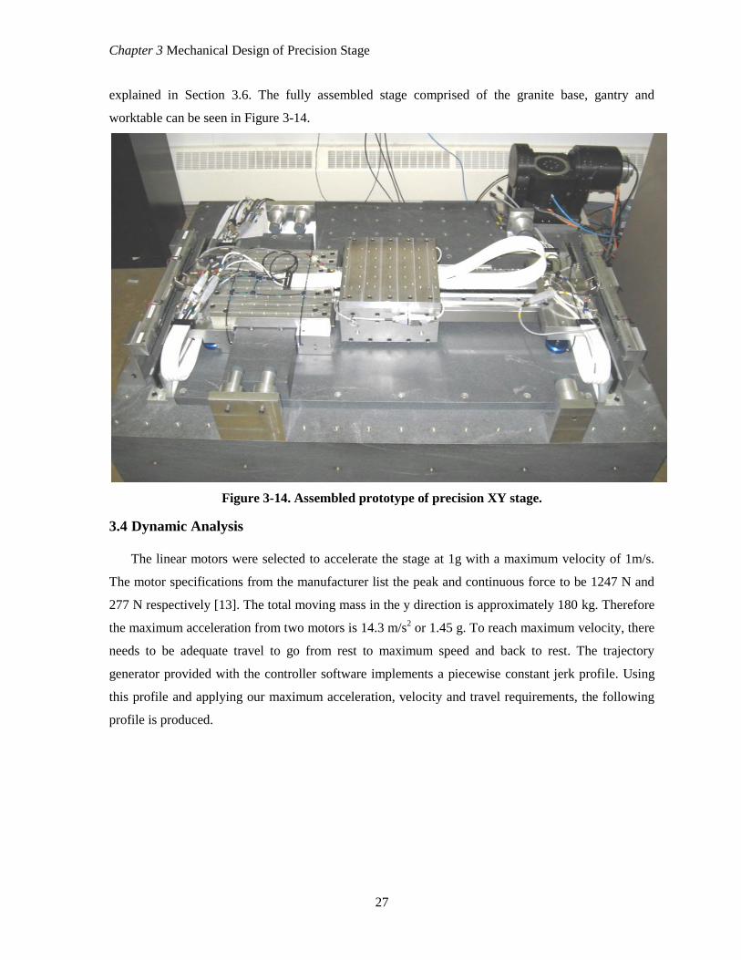
explained in Section 3.6. The fully assembled stage comprised of the granite base, gantry and
worktable can be seen in Figure 3-14.
Figure 3-14. Assembled prototype of precision XY stage.
3.4 Dynamic Analysis
The linear motors were selected to accelerate the stage at 1g with a maximum velocity of 1m/s.
The motor specifications from the manufacturer list the peak and continuous force to be 1247 N and
277 N respectively [13]. The total moving mass in the y direction is approximately 180 kg. Therefore
the maximum acceleration from two motors is 14.3 m/s2 or 1.45 g. To reach maximum velocity, there
needs to be adequate travel to go from rest to maximum speed and back to rest. The trajectory
generator provided with the controller software implements a piecewise constant jerk profile. Using
this profile and applying our maximum acceleration, velocity and travel requirements, the following
profile is produced.

Chapter 3 Mechanical Design of Precision Stage
28
Figure 3-15. Example of trajectory profile
It can be seen from the figure that maximum velocity is reached for 200 mm of travel within the
entire 300 mm range of travel. The following table lists some key values related to the machine and
its dynamic performance.
Table 3-1. List of dynamic values of the machine.
X Y
Mass [kg] 33 180
Max Motor Force [N] 1247 2494
Maximum Acceleration [g] 3.85 1.45
Maximum Velocity [m/s] 1.0 1.0
Maximum Stroke [m] 0.3 0.3
Feedback Resolution [nm] 0.97 0.97
Machine vibration is an area which cannot be ignored and must be studied in parallel with rigid
body dynamics. Vibrations can lead to loss of positional accuracy, weakening of the machine’s
structure as well as controller instability. An assessment of different sources of vibration was
performed to attempt to identify the dynamics of the stage. Understanding the source of vibration can
aid in determining solutions to diminish its effects on the accuracy of the machine.
The gantry beam was identified as a likely source of vibration with detrimental effects to
accuracy as well as stability of the machine. Two areas were analyzed, which are the rigid body yaw
vibration and the first bending mode of the beam. The frequency of the yaw vibration will be referred
to as the yaw frequency. The natural yaw frequency is calculated with Equation (3.1).

Chapter 3 Mechanical Design of Precision Stage
29
𝜔𝑛 =1
2𝜋 𝑘𝜃
𝐼 (3.1)
Where,
𝑘𝜃 is the yaw stiffness 𝑁∙𝑚
𝑟𝑎𝑑
𝐼 is the Moment of Inertia 𝑘𝑔 ⋅ 𝑚2
The yaw stiffness of the gantry can be calculated by relating the stiffness of the bearings to an
equivalent angular stiffness. Equation (3.2) is the definition of linear stiffness while Equation (3.3) is
angular stiffness.
𝑘 =
𝐹
𝛿 (3.2)
𝑘𝜃 =
𝑀
𝜃 (3.3)
Assuming small angles, the following diagram is used to relate Equations (3.2) and (3.3). The
forces applied by the linear springs can be converted to an equivalent moment and the linear
deflection can be related to an angular deflection as noted in Equation (3.4). The air bearings apply
unidirectional stiffness which only acts during compression of the air gap. Therefore, during angular
vibration of the gantry, it is assumed that only two bearings provide stiffness during yaw.
(a) (b)
Figure 3-16. Relationship between the 4 preloaded air bearings and a torsional spring. (a)
overall machine diagram and (b) geometrical relationship
𝑘𝜃 =𝑀
𝜃=
2𝐹 𝑑2
𝛿
𝑑2
(3.4)
Simplifying Equation (3.4) to include the stiffness of the linear bearings yields,

Chapter 3 Mechanical Design of Precision Stage
30
𝑘𝜃 = 2𝑘𝑏
𝑑
2
2
(3.5)
The moment of inertia in Equation (3.1) is calculated about the torsional spring in Figure 3-16.
Due to the complexity of the stage, the inertia is approximated using CAD software. The moment of
inertia of the worktable is determined using CAD and the parallel axis theorem to translate the inertia
to the same location as the gantry. The following table lists the required values to solve Equation
(3.6).
Table 3-2. List of required values to calculate the natural frequency of the yaw vibration of the
gantry.
Description Symbol Value Units
Bearing Stiffness [30] 𝑘𝑏 324 𝑁/𝑢𝑚 Distance between bearings 𝑑 0.25 𝑚 Moment of Inertia of Gantry about bearings 𝐼𝑔 46.63 𝑘𝑔𝑚2
Moment of Inertia of Table about its center 𝐼𝑡 0.6058 𝑘𝑔𝑚2
Distance from table to gantry moment of inertia 𝑑𝑡 0.4 – 0.7 𝑚
Mass of worktable 𝑚𝑡 33 𝑘𝑔
𝜔𝑛 =1
2𝜋
2𝑘𝑏 𝑑2
2
𝐼𝑔 + 𝐼𝑡 + 𝑚𝑡𝑑𝑡2
𝝎𝒏 = 𝟔𝟕 𝑯𝒛, 𝑓𝑜𝑟 𝑑𝑡 = 0.55
(3.6)
A natural frequency of 67 Hz has been calculated for the yaw vibration. It should be noted that
this frequency was also spotted in the Frequency Response measurement acquired in Chapter 4.
The first bending mode is modeled by considering the beam as a simple fixed-free cantilever.
Equation (3.7) calculates the first bending mode frequency [32].
𝜔𝑛 =3.52
2𝜋
𝐸𝐼
𝑤𝐿4 (3.7)
Where,
𝐸 = Modulus of elasticity (𝑃𝑎)
𝐼 = Area moment of inertia (𝑚4)
𝑤 = Mass per length 𝑘𝑔
𝑚
𝐿 = Length of beam (𝑚)
Table 3-3 lists the terms required for the calculation of the first bending mode of the beam.

Chapter 3 Mechanical Design of Precision Stage
31
Table 3-3. List of terms required for calculating the first bending mode of the gantry beam.
Description Symbol Value Units
Modulus of elasticity 𝐸 193 𝐺𝑃𝑎
Area moment of inertia 𝐼 =𝑏3
12 2.624x10
-5 𝑚4
Beam width 𝑏 0.054 𝑚 Beam height 0.18 𝑚
Beam length 𝐿 0.87 𝑚
Mass per length 𝑤 77.76 𝑘𝑔/𝑚
𝜔𝑛 =3.52
2𝜋
𝐸
𝑏3
12
𝑤𝐿4
𝜔𝑛 = 190𝐻𝑧
(3.8)
This analysis is an approximation and will be further analyzed during the frequency response
identification experiments in Chapter 4.
3.5 Static Stiffness Analysis
The static stiffness of the machine is derived from the stiffness of the air bearings, linear motors,
and the bending stiffness of the gantry beam. An additional analysis is performed on the pitch of the
gantry during constant acceleration. The air bearing stiffness, as reported by the manufacturer, for
each bearing at the 5 µm nominal fly height is listed in the table below.
Table 3-4. Stiffness values of air bearings used on the machine.
Bearing Size Symbol Stiffness [N/µm] [30]
80 mm (Round) 𝑘1 114
75 mm x 150 mm (Rectangular) 𝑘2 324
50 mm x 100 mm (Rectangular) 𝑘3 110
The stiffness is calculated in the x and y axes using Figure 3-17.

Chapter 3 Mechanical Design of Precision Stage
32
Figure 3-17. Stiffness diagram of the machine to analytically determine the overall stiffness in
the x and y directions.
The total stiffness in the x-axis is calculated assuming the springs act in series. A similar calculation
is made for the y-axis, however, the pitch stiffness acts in parallel.
𝑘𝑥−1 = 2𝑘2
−1 + 𝑘𝑠𝑒𝑟𝑣𝑜−1 (3.9)
𝑘𝑦−1 = 2𝑘3
−1 + 2𝑘𝑠𝑒𝑟𝑣𝑜−1 + 𝑘𝑏𝑒𝑛𝑑𝑖𝑛𝑔
−1 (3.10)
The additional 𝑘𝑏𝑒𝑛𝑑𝑖𝑛𝑔 term for the y-axis stiffness is related to the bending of the beam under
static load. The beam can be represented by a torsion-pinned configuration as shown in Figure 3-18.
Figure 3-18. Static bending diagram of the gantry beam.
The torsion spring represents the yaw stiffness of the four preloaded air bearings, as mentioned in
Section 3.4, and the pinned joined on the right assumes the secondary motor is powered, providing
infinite static stiffness due to the implementation of integral action in the control law. The elastic
curve formula is used to derive the equation of the deflection for the beam. Since the formula is 4th
order, four boundary conditions are required to calculate the integration constants.
𝐸𝐼
𝑑4𝑣
𝑑𝑥4= 𝑤 𝑥 (3.11)
𝑣 0 = 0 𝑣 𝐿 = 0
𝑣 ′′ 𝐿 = 0
𝑣 ′′ 0 =𝑘𝜃
𝐸𝐼𝑣 ′ 0
(3.12)

Chapter 3 Mechanical Design of Precision Stage
33
Where,
𝑣 = Deflection (𝑚)
𝑤 = Force (𝑁)
𝐸 = Modulus of Elasticity (𝑃𝑎)
𝐼 = Moment of Inertia (𝑚4)
𝑘𝜃 = Torsion Stiffness Constant 𝑁∙𝑚
𝑟𝑎𝑑
Solving for 𝑣 𝑥 gives
𝑣 𝑥 =
𝑃
288 𝐸𝐼 2 + 96𝐸𝐼𝑘𝜃𝐿 𝑥 𝑘𝜃𝐿 9𝐿 − 11𝑥 𝑥 + 6𝐸𝐼 3𝐿2 − 4𝑥2
− 2 3𝐸𝐼 + 𝑘𝜃𝐿 𝐿 − 2𝑥 3𝐻 −𝐿 + 2𝑥
(3.13)
To determine the minimum stiffness, the point which has the most deflection must be determined. To
find the point, the equation for slope of the beam (𝑣 ′(𝑥)) is set equal to zero and solved for 𝑥. It was
found that the maximum deflection occurs at 0.513𝐿. To simplify the mathematics involved to
determine the bending stiffness, it is assumed that the maximum deflection occurs at 𝐿/2. Therefore,
the equation for the bending stiffness of the beam is:
𝑘𝑏𝑒𝑛𝑑𝑖𝑛𝑔 =𝑃
𝑣 𝐿2
=768𝐸𝐼 3𝐸𝐼 + 𝑘𝜃𝐿
𝐿3 48𝐸𝐼 + 7𝑘𝜃𝐿 (3.14)
The torsion stiffness 𝑘𝜃 was calculated using Equations (3.2) - (3.5).
The servo stiffness is derived from the bandwidth of the controller which can be calculated as
follows:
𝑘𝑠𝑒𝑟𝑣𝑜 = 𝑚𝜔𝑏𝑤2 (3.15)
The stiffness from each axis was analyzed under three cases with varying servo stiffness. Case 1
assumes a 30 Hz servo bandwidth, which is common on most machine tool drives. Case 2 assumes
100 Hz servo bandwidth, which is common in high performance servo-drives. Case 3 assumes infinite
dc stiffness due to integral action from the controller. This assumption is realized by analyzing a
simple first order system with a PID controller.

Chapter 3 Mechanical Design of Precision Stage
34
Figure 3-19. Block diagram of a first order system with a PID controller
Simplifying the block diagram and solving for the output in terms of the inputs produces,
𝑋 𝑠 =𝐾𝑑𝑠
2 + 𝐾𝑝𝑠 + 𝐾𝑖
𝑠3 + 𝑏 + 𝐾𝑑
𝑚𝑠2 +
𝐾𝑝𝑚
𝑠 +𝐾𝑖𝑚
𝑋𝑟 𝑠
+
1𝑚
𝑠
𝑠3 + 𝑏 + 𝐾𝑑
𝑚𝑠2 +
𝐾𝑝𝑚
𝑠 +𝐾𝑖𝑚
𝑑(𝑠)
(3.16)
During a situation where the stage is under control and at rest, the reference input (𝑋𝑟) is zero.
Therefore the disturbance (𝑑) input is the remaining factor which determines the stiffness of the
controller. Plotting the disturbance transfer function in the frequency domain produces the profile in
Figure 3-20. For a static load disturbance, the frequency can be assumed to be ~0 Hz and according to
the figure, the magnitude at 0 Hz approaches zero. Therefore, static stiffness for a controller with
integral action can be assumed to be infinite.

Chapter 3 Mechanical Design of Precision Stage
35
Figure 3-20. Disturbance transfer function of a PID controller for a 1st order model system.
During constant acceleration of the gantry, a moment load is applied due to the motors not acting
along the center of mass, which causes the gantry to pitch. This rotation causes a linear deflection at
the encoder heads, which is recorded as displacement error. The value of this displacement can be
determined by analyzing a free body diagram of the gantry in Figure 3-21.
Figure 3-21. Free body diagram of gantry pitch motion during constant acceleration
The force equations were calculated using the center of mass as the reference point.
𝐹𝑧 = 0 = 𝐹𝑏1 + 𝐹𝑏2 − 𝑚𝐺𝑔 (3.17)

Chapter 3 Mechanical Design of Precision Stage
36
𝐹𝑦 = 𝑚𝐺𝑎 = 𝐹𝑚 − 𝐹𝑡 (3.18)
𝑇𝑥 ≅ 0 = 𝐹𝑚 𝑧𝑐𝑜𝑚 − 𝑧𝑚 − 𝐹𝑡 𝑧𝑐𝑜𝑚 − 𝑧𝑡 − 𝐹𝑏1𝑦𝑏1 + 𝐹𝑏2𝑦𝑏2 (3.19)
Solving the system of equations for 𝐹𝑏1 and 𝐹𝑏2, results in the following equation.
𝐹𝑏1,𝑏2 =𝑚𝐺𝑔
2±
𝑎
2𝑦𝑏1,𝑏2
𝑚𝐺 + 𝑚𝑡 𝑧𝑐𝑜𝑚 − 𝑧𝑚 − 𝑚𝑡(𝑧𝑐𝑜𝑚 − 𝑧𝑡) (3.20)
Table 3-5 lists the values required to calculate the load of the bearings during 1 g acceleration.
Table 3-5. Gantry pitch parameter values
Parameter Value Units
𝑔 9.81 𝑚/𝑠2
𝑎 9.81 𝑚/𝑠2
𝑚𝐺 142 𝑘𝑔
𝑚𝑡 33 𝑘𝑔
𝑦𝑏1,𝑏2 166 𝑚𝑚
𝑧𝑐𝑜𝑚 85.0 𝑚𝑚
𝑧𝑚 50.0 𝑚𝑚
𝑧𝑡 67.5 𝑚𝑚
The load of the each bearing was found to be 𝐹𝑏1 = 430 N, and 𝐹𝑏2 = 266 N. These values can
be used to determine the fly height of the bearings by analyzing the lift-load curve, provided by the
manufacturer, in Figure 3-22.
Figure 3-22. Lift-load curve for 80mm diameter air bearings [30]

Chapter 3 Mechanical Design of Precision Stage
37
It can be seen from the figure that 𝛿1 = 13 µm and 𝛿2 = 17 µm. The deflection of the encoder
head is calculated using Equation (3.21) with 𝑧𝑒𝑛𝑐 = 140 mm.
𝛿2 − 𝛿1
𝑦𝑏1 + 𝑦𝑏2=
𝛿3
𝑧𝑒𝑛𝑐
𝛿3 = 1.7 𝑢𝑚
(3.21)
Therefore, during 1 g acceleration, a 1.7 µm measurement error is created by the deflection of the
encoder head. In later sections, an acceleration of 0.2 g is used for analysis and the encoder head will
experience a measurement error of 0.34 µm. Table 3-6 presents the stiffness in each axis for all 3
cases.
Table 3-6. Overall stiffness of the x and y axes for 3 different servo bandwidths.
Case 1 Case 2 Case 3
X Y X Y X Y
SERVO STIFFNESS
𝑓𝑠𝑒𝑟𝑣𝑜 [Hz] 30 30 100 100
𝜔𝑠𝑒𝑟𝑣𝑜 [rad/sec] 188 188 628 628
𝑚𝑠𝑒𝑟𝑣𝑜 [kg] 33.0 175 33.0 175 33.0 175
𝑘𝑠𝑒𝑟𝑣𝑜 [N/µm] 1.17 6.22 13.0 69.1
BEARING STIFFNESS
𝑘𝑏𝑒𝑎𝑟𝑖𝑛𝑔 [N/µm] 648 220 648 220 648 220
BENDING STIFFNESS
𝐸 [GPa] 193 193 193
𝐼 [m4] 2.62x10
-5 2.62x10
-5 2.62x10
-5
𝑘𝜃 [Nm/rad] 1.01x10⁷
1.01x10⁷ 1.01x10
7
𝐿 [m] 0.870 0.870 0.870
𝑘𝑏𝑒𝑛𝑑𝑖𝑛𝑔 [N/µm] 422 422 422
TOTAL STIFFNESS
𝒌 [N/µm] 1.17 5.97 12.8 46.8 648 145
The total stiffness of the axes is highly influenced by the servo stiffness of the motors. Therefore,
dynamic identification and controller design are crucial in order to verify the design specification of
50 N/µm. The controller design is discussed in detail in Chapter 4.
3.6 Thermal Analysis
Thermal analyses of machine tools and their environment are significant to facilitate their
accuracy specifications. Traditional machine tools require a warm up period which has the machine
powered and moving in order to reach thermal equilibrium. The time required can be several hours in
order to reach this state [1]. As the machine warms up, the motors, guideways, bearings, etc. heat up
and expand which causes positioning errors. This issue is typically avoided since the machines are

Chapter 3 Mechanical Design of Precision Stage
38
run on long shifts which can last for days at a time therefore the machine is at or near thermal
equilibrium. The design of the machine can also help reduce the effect of thermal errors. A symmetric
machine structure will typically expand in a symmetric and uniform fashion. If the encoder heads are
positioned along the axis of symmetry, they become insensitive to thermal effects. However, an
asymmetric structure expands in a more complicated manner, which can make it difficult to measure
and compensate for any positional errors. For machines composed of different materials, thermal
variation causes warping between the components. For example, if an aluminum and steel plate are
bolted together and their temperatures are raised, stress will be created between the two components
since the aluminum expands more than steel. A warping effect will be seen due to this thermally
induced stress. The machine in this thesis uses aluminum, stainless steel, glass and granite. These all
have different coefficients of expansion. Therefore, it is imperative to mitigate all sources of thermal
error at their source, which in this case are the environment and the linear motors.
The expansion of the stage due to a change in temperature was estimated to determine the
magnitude of positional errors which may be observed. The following table outlines which areas of
the stage are sensitive and which do not require analysis.
Table 3-7. Areas of the stage which are sensitive to thermal changes.
X Y
Gantry Structure sensitive insensitive
Worktable Structure insensitive insensitive
Gantry encoder scales insensitive sensitive
Worktable encoder scale sensitive insensitive
The gantry is asymmetric about the y-axis, since the guideway is located on the left with the beam
extending to the right. Temperature changes will expand the beam, which will shift the x-axis encoder
scale. Therefore the gantry is sensitive to thermal changes along the x-axis. Since the gantry is
symmetric about the x-axis and the encoder heads are located along the axis of symmetry, the gantry
is insensitive along the y-axis. The worktable structure is symmetric about both axes and is therefore,
insensitive to thermal changes.
The encoder scales are sensitive along their direction of measurement. This is due to the glass
scale expanding as the temperature increases. The coefficient of thermal expansion for the glass scale
is 8 ppm/°C. The scales are held in a floating mounts, hence in this analysis they are assumed to be
fixed in the middle with both ends expanding outwards. With a range of travel of 150 mm to each
side, the error will be 1.35 µm/°C at the furthest position from center. The gantry beam has a
coefficient of thermal expansion of 17.3 ppm/°C and it is assumed to be fixed at the left side. The
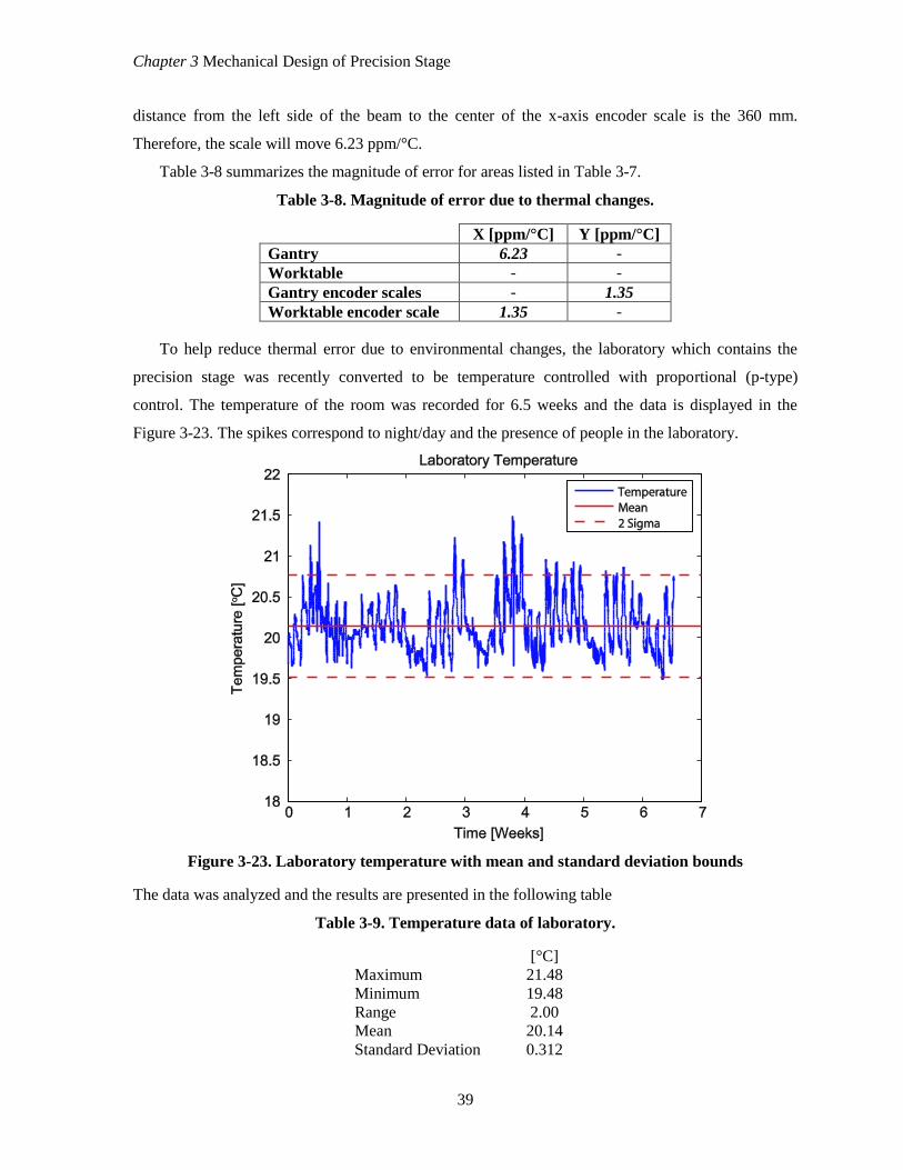
Chapter 3 Mechanical Design of Precision Stage
39
distance from the left side of the beam to the center of the x-axis encoder scale is the 360 mm.
Therefore, the scale will move 6.23 ppm/°C.
Table 3-8 summarizes the magnitude of error for areas listed in Table 3-7.
Table 3-8. Magnitude of error due to thermal changes.
X [ppm/°C] Y [ppm/°C]
Gantry 6.23 -
Worktable - -
Gantry encoder scales - 1.35
Worktable encoder scale 1.35 -
To help reduce thermal error due to environmental changes, the laboratory which contains the
precision stage was recently converted to be temperature controlled with proportional (p-type)
control. The temperature of the room was recorded for 6.5 weeks and the data is displayed in the
Figure 3-23. The spikes correspond to night/day and the presence of people in the laboratory.
Figure 3-23. Laboratory temperature with mean and standard deviation bounds
The data was analyzed and the results are presented in the following table
Table 3-9. Temperature data of laboratory.
[°C]
Maximum 21.48
Minimum 19.48
Range 2.00
Mean 20.14
Standard Deviation 0.312

Chapter 3 Mechanical Design of Precision Stage
40
The goal is to have the room maintain a constant temperature of 20°C ± 0.2°C which the
controller is currently not achieving. It is believed that a digital proportional-integral controller will
improve the accuracy of the temperature control, particularly in coping with internal and external
disturbances due to room occupancy and outside temperature changes.
As mentioned in Section 3.3, internally cooled couplings are designed to remove any heat
generated by the linear motors. The y-axis couplings were designed by Carlton Banks as a 4th year
design project [33]. The purpose was to design the coupling such that the heat dissipated by the motor
would be removed by the glycol, which is cycled through the internal channels of the coupling. The
criteria for the design for the x and y-axis couplings are:
1. Align, position and secure the linear motor to the coupling
2. Align, position and secure the coupling to the stage
3. Include inlet and outlet ports for glycol
4. Configure internal cooling channels to dissipate the maximum heat generated by motor
5. Design must be leak proof under 100 psi internal pressure
6. Coupling must be handled as single unit (ie. The seal cannot be broken during disassembly
of stage)
The y-axis design is presented in Figure 3-24.
Figure 3-24. Y-axis coupling design
The x-axis coupling is presented in Figure 3-25.

Chapter 3 Mechanical Design of Precision Stage
41
Figure 3-25. X-axis coupling design
The couplings were analyzed before production to verify their effectiveness to remove heat under
maximum thermal loading. The following assumptions were used in the analysis:
- Uniform volumetric heating of the motor.
- All exposed surfaces of the motor and coupling are insulated (worst case).
- Constant and uniform heat transfer between the coupling and glycol.
- Glycol is always at 20°C.
The motors coils have a maximum heat dissipation of 131 W and volume of 214 cm3. Therefore,
they have a volumetric heating coefficient of 0.612 W/cm3. Figure 3-26 displays the results of the
analysis for the y-axis coupling. It is important to note the temperature of the surface which is in
contact with the stage.
Figure 3-26. Thermal analysis of y-axis coupling
The same analysis was performed on the x-axis coupling, which is shown in Figure 3-27.

Chapter 3 Mechanical Design of Precision Stage
42
Figure 3-27. Thermal analysis of x-axis coupling
It can be seen from the figures that the surface in contact with the stage maintains a temperature of
20°C. Therefore, the effect of thermal errors from the motors can be considered negligible.
3.7 Error Budget
This section presents an error budget for the precision stage and outlines major sources of error
for the machine [34]. The amount of error contributed by each source is quantified and critical areas
are determined. Efforts can then be made to develop solutions to minimize individual errors. Each of
the following sub-sections focuses on a particular source of error and attempts to quantify its impact
on the overall accuracy. The reader is referred to Section 2.4 for definitions and a full explanation of
linear, straightness and angular errors.
3.7.1 Linear Positional Error
The linear error for each axis consists of encoder scale error, the resolution of the encoders and
the uncertainty of the encoder signal. The encoder scales have error from imperfections within the
grating. Each encoder scale is tested for its positional error and a certificate with the error profile is
provided to the customer. The scale error for the scales used with the stage is 0.79 µm. A resolution
of 0.97nm is achieved by interpolating the 4 µm wavelength signal in 4096 sub-divisions. However,
the uncertainty within one signal period is 0.044um, as provided by the manufacturer. The error
within one signal period is critical for both the accuracy of positioning, as well as velocity control
during a slow and constant velocity traverse of an axis. Metrology experiments can measure the
encoder scale error and since these errors are mostly repeatable, compensation can be applied which

Chapter 3 Mechanical Design of Precision Stage
43
can reduce the error by 100 times. The uncertainty of the signal and encoder resolution cannot be
compensated.
3.7.2 Straightness Error
Straightness error refers to the unwanted motion in one of the two directions orthogonal to the
direction of a linear axis commanded to move along a (nominal) straight-line trajectory. Typically,
these are referred to vertical and horizontal straightness errors. However, it depends on the setup of
the system and its orientation within the machine. The straightness error is directly dependent on the
geometry of the guideways. For the Y-axis, the gantry moves along the base granite surface and
granite guideway. The X-axis is guided by the base granite surface and the stainless steel gantry
beam. These surfaces were built with a specified tolerance of 2 µm/300 mm. Therefore the maximum
expected straightness error is 2um since the range of travel is 300 mm. Straightness errors are
repeatable and compensation of their error is possible. As with linear error, metrology measurements
can determine the error profile which can be used to reduce the error.
3.7.3 Angular Error
Angular error refers to the three unwanted rotational movements of a moving component
commanded to move along a (nominal) straight-line trajectory. Typically, these are referred to as
yaw, pitch and roll errors. These errors are created from the contours of the guideways. The
maximum angular error for each axis can be calculated from the maximum slope of the guideways
which is 2 µm/300 mm or 6.7 nm/mm. To relate angular error to the other sources of error, it must be
converted into linear units. This is accomplished by selecting a point of interest (usually the tool tip or
reference point on a workpiece) and an axis of rotation for each angular degree of freedom. The
distance between the two is the lever arm and then the angular errors can be converted into small
linear displacements. The point of interest was chosen to be the center of the top plate of the
worktable. The following assumptions are made when calculating the linear displacements.
- Pitch of the worktable contributes to displacement in y.
- Roll of the worktable contributes to displacements in x.
- Yaw of the worktable does not contribute to displacements.
- Pitch of the gantry does not contribute to displacements (since the gantry and table are
vertically decoupled from each other).
- Roll of the gantry does not contribute to displacements (since the gantry and table are
vertically decoupled from each other).
- Yaw of the gantry contributes to displacements in the y. Its x-axis error contribution is
negligible due to it being a cosine error.
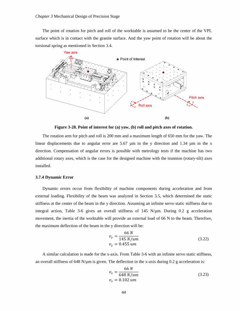
Chapter 3 Mechanical Design of Precision Stage
44
The point of rotation for pitch and roll of the worktable is assumed to be the center of the VPL
surface which is in contact with the granite surface. And the yaw point of rotation will be about the
torsional spring as mentioned in Section 3.4.
(a) (b)
Figure 3-28. Point of interest for (a) yaw, (b) roll and pitch axes of rotation.
The rotation arm for pitch and roll is 200 mm and a maximum length of 650 mm for the yaw. The
linear displacements due to angular error are 5.67 µm in the y direction and 1.34 µm in the x
direction. Compensation of angular errors is possible with metrology tests if the machine has two
additional rotary axes, which is the case for the designed machine with the trunnion (rotary-tilt) axes
installed.
3.7.4 Dynamic Error
Dynamic errors occur from flexibility of machine components during acceleration and from
external loading. Flexibility of the beam was analyzed in Section 3.5, which determined the static
stiffness at the center of the beam in the y direction. Assuming an infinite servo static stiffness due to
integral action, Table 3-6 gives an overall stiffness of 145 N/µm. During 0.2 g acceleration
movement, the inertia of the worktable will provide an external load of 66 N to the beam. Therefore,
the maximum deflection of the beam in the y direction will be:
𝑣𝑦 =
66 𝑁
145 𝑁/𝑢𝑚
𝑣𝑦 = 0.455 𝑢𝑚
(3.22)
A similar calculation is made for the x-axis. From Table 3-6 with an infinite servo static stiffness,
an overall stiffness of 648 N/µm is given. The deflection in the x-axis during 0.2 g acceleration is:
𝑣𝑥 =
66 𝑁
648 𝑁/𝑢𝑚
𝑣𝑥 = 0.102 𝑢𝑚
(3.23)

Chapter 3 Mechanical Design of Precision Stage
45
Accelerating the worktable at 0.2 g along the y-axis is predicted to result in a displacement of
0.455 µm while a similar acceleration in x will result in a displacement of 0.102 µm. This
deformation, however, is expected to be repeatable and will be modeled with the intention of applying
real-time compensation. Additionally, the pitch of the gantry during 0.2 g acceleration will result in
approximately 0.34 µm deflection of the encoder head in the y-axis.
3.7.5 Servo Error
Servo errors are a type of dynamic error which occurs during accelerations of the machine. It is
also known as following error or tracking error. A simulation was performed to approximate the servo
error expected for the x and y axes. A first order model with inertia and viscous friction coefficients
was used to represent the mechanics of the system. The controller used is a Proportional-Integral-
Derivative (PID) controller with feedforward acceleration and velocity. A reasonable controller
bandwidth was chosen to be 30 Hz which is typical for most ball-screw drives. Higher bandwidth
controllers (100 Hz) are possible with direct drive linear motors. However, the lower bandwidth was
selected to represent a worst case and more realistic scenario. The feedforward estimates assume that
the mass and friction values are identified with minimal uncertainty. A trajectory selected for the
simulation is 200 mm travel, 0.2 m/s velocity, and 0.2 g acceleration with a 50 m/s3 jerk-continuous
profile. This trajectory will be used during actual tracking tests in Chapter 4. The results of the
simulation are in Figure 3-29 and the peak servo error was found to be 0.1 µm for both axes.
Figure 3-29. Simulated servo error

Chapter 3 Mechanical Design of Precision Stage
46
3.7.6 Thermal Error
A thermal analysis of the stage was performed in Section 3.6 which quantified how the stage
expands with changes in temperature. It also verified the effectiveness of the cooling couplings which
will remove the heat generated by the motors. The temperature of the environmentally controlled
laboratory was recorded and plotted in Figure 3-23. The maximum range of temperature change was
noted to be ± 1°C. Using this data in conjunction with Table 3-8, a maximum thermal error can be
calculated. The error in the x direction consists of the expansion of the gantry beam and the worktable
encoder scale. Therefore, a maximum error in the x direction is 7.58 µm and 1.35 µm in the y
direction. However, further temperature control improvements are currently planned which will lower
the temperature range to ± 0.2°C. Therefore, the error due to thermal change will be 1.52 µm in the x-
axis and 0.27 µm in the y-axis.
3.7.7 Overall Error Budget
The error budget has been presented and a range of topics have been analyzed for their maximum
contribution to error of the machine. Linear, straightness and angular errors were determined through
geometric characteristics of the guideways while dynamic and thermal errors were calculated
analytically. The results are presented in the following table which summarizes all of the errors for
the x, y and z axes. [34]

Chapter 3 Mechanical Design of Precision Stage
47
Table 3-10. Predicted Error Budget.
Error Magnitude (nm)
Without Geometry
Compensation
With Geometry
Compensation
X Y Z X Y Z
Linear
Encoder resolution 0.97 0.97 0.97 0.97
Scale 790 790 79 79
Encoder signal 44 44 44 44
Straightness
Y Guide 2000 200 200
X Guide 2000 2000 200 200 200
Angular
Y Guide 0 4330 0 433
X Guide 1340 1340 134 134
Dynamic (0.2 g acceleration)
Servo 100 100 100 100
Air Bearings 102 300 15 45
Beam 155 23
Gantry Pitch 340 51
Thermal
Friction 0 0 0 0 0 0
Drive System 0 0 0 0 0 0
Environment (20 ± 0.2°C) 1520 270 0 1520 270 0
Static Error
Arithmetic Sum (EA) 5695 8775 2000 2178 1361 200
RMS1 Sum (ER) 1206 1899 2000 635 229 200
Mean ((EA + ER)/2) 3451 5337 2000 1406 795 200
Maximum Resultant Error ET = 5.87 µm ET = 1.63 µm
Static + Dynamic Error
Arithmetic Sum (EA) 5897 9670 2000 2293 1580 200
RMS Sum (ER) 1046 1522 2000 551 186 200
Mean ((EA + ER)/2) 3471 5596 2000 1422 883 200
Maximum Resultant Error ET = 6.11 µm ET = 1.69 µm
It can be seen that the largest contributor to the overall error of the machine environment thermal
error. Further study into temperature control of the laboratory should be initiated in order to improve
the accuracy of the machine.
1 Assumes normal probability for each error about its mean value
1 Compensation indicates the correction of repeatable geometric & dynamic errors by shifting the position
Chapter 3 Mechanical Design of Precision Stage
48
3.8 Conclusion
An ultra-precision planar stage concept and prototype has been designed and presented in this
chapter. The T-type gantry and worktable configuration achieves an overall work area of 300 mm x
300 mm with a maximum velocity of 1 m/s and maximum acceleration of 1 g. The stage is supported
by porous carbon air bearings on a precision ground granite base and actuation is achieved through
direct drive linear motors with high resolution feedback of 1 nm. A VPL is utilized underneath the
worktable to provide high vertical and pitch stiffness as well as decouple the gantry beam from
vertical loads. A dynamic analysis of the gantry yielded a natural yaw frequency of 67 Hz and the
first bending mode of the beam was calculated to be 190 Hz. These modes will be compared to
experimental data in Chapter 4. The static stiffness of the machine was determined for the x and y
axes by determining the servo, bearing and beam stiffness. Assuming the stiffness’s act in series and
the controller has integral action, a theoretical overall stiffness of 648 N/µm and 145 N/µm were
calculated for the x and y axes respectively.
An additional thermal analysis was performed to quantify the effects of thermal influences on the
machine structure and accuracy. The x-axis was identified to be most sensitive to thermal effects due
to the elongation of the gantry beam and encoder scale. The maximum relative expansion coefficient
was determined to be 7.58 µm/°C in the x direction and 1.35um/°C in the y. Internally cooled
couplings were designed to mitigate thermal effects due to the linear motors. Their effectiveness was
verified through finite element analysis which proved the couplings were successful at keeping the
stage side of the coupling at 20°C.
An overall error budget was presented which combined geometric, dynamic and thermal errors to
determine an overall error of the machine. With geometric compensation, the error was predicted to
be 1.69 µm with the main contributor being thermal errors from the environment.

49
Chapter 4
Statics, Dynamics and Controls
4.1 Introduction
In this chapter, the dynamics are experimentally identified and high performance controllers are
developed for the x- and y-axis drive systems. Section 4.2 focuses on the static stiffness of the axes
and compares the findings to the theoretical stiffness values calculated in Chapter 3. Section 4.3
performs frequency domain identification experiments to characterize the dynamics of the stage.
Parameter identification for models and controller design is performed in Section 4.4. A Multi-input-
multi-output (MIMO) model is established for the y-axis due to the strong coupling between the
primary and secondary motors. A loop-shaping controller for the x-axis is designed and a
multivariable state-feedback controller is designed for the y-axis. The designs are verified through
stability analyses and tracking tests. The conclusions are presented in Section 4.5.
4.2 Static Stiffness
In Section 3.5, a static stiffness analysis was performed, which attempted to analytically
determine the stiffness of the stage in the x- and y-axes. Theoretical stiffness values were found to be
648 and 145 N/µm in the x- and y-axes respectively. The experimental stiffness values will be lower
due to unaccounted flexibilities in the system. The actual static stiffness was measured using dead
weights, which pull laterally on the stage via a cable and pulley system. The stiffness was measured
along a grid pattern inside the workspace, simulating a load from a spindle located at the center of the
workspace for the x-axis. The stiffness in the x-direction at each location was measured and is
presented in Figure 4-1.

Chapter 4 Statics, Dynamics and Controls
50
Figure 4-1. X-axis stiffness grid pattern and results
The stiffness in the y-direction at each location was measured and is presented in Figure 4-2.
Figure 4-2. Y-axis stiffness grid pattern and results
The actual stiffness was measured to be much less than the theoretical stiffness. This is due to the
pitch stiffness of the worktable and ultimately, the VPL and its bolted interface. The dead weight load
is applied on the top surface of the worktable creating, a pitch load. Although this creates a moment
on the table, it is a more realistic stiffness measurement since this is the location where cutting forces
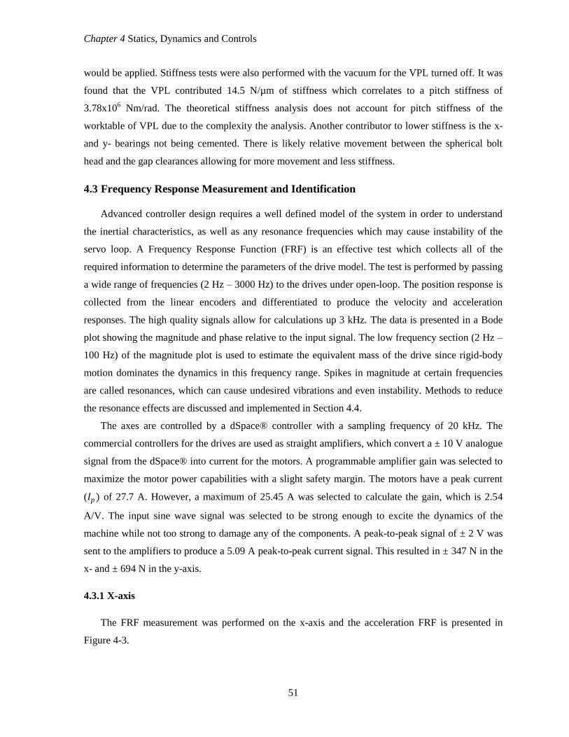
Chapter 4 Statics, Dynamics and Controls
51
would be applied. Stiffness tests were also performed with the vacuum for the VPL turned off. It was
found that the VPL contributed 14.5 N/µm of stiffness which correlates to a pitch stiffness of
3.78x10⁶ Nm/rad. The theoretical stiffness analysis does not account for pitch stiffness of the
worktable of VPL due to the complexity the analysis. Another contributor to lower stiffness is the x-
and y- bearings not being cemented. There is likely relative movement between the spherical bolt
head and the gap clearances allowing for more movement and less stiffness.
4.3 Frequency Response Measurement and Identification
Advanced controller design requires a well defined model of the system in order to understand
the inertial characteristics, as well as any resonance frequencies which may cause instability of the
servo loop. A Frequency Response Function (FRF) is an effective test which collects all of the
required information to determine the parameters of the drive model. The test is performed by passing
a wide range of frequencies (2 Hz – 3000 Hz) to the drives under open-loop. The position response is
collected from the linear encoders and differentiated to produce the velocity and acceleration
responses. The high quality signals allow for calculations up 3 kHz. The data is presented in a Bode
plot showing the magnitude and phase relative to the input signal. The low frequency section (2 Hz –
100 Hz) of the magnitude plot is used to estimate the equivalent mass of the drive since rigid-body
motion dominates the dynamics in this frequency range. Spikes in magnitude at certain frequencies
are called resonances, which can cause undesired vibrations and even instability. Methods to reduce
the resonance effects are discussed and implemented in Section 4.4.
The axes are controlled by a dSpace® controller with a sampling frequency of 20 kHz. The
commercial controllers for the drives are used as straight amplifiers, which convert a ± 10 V analogue
signal from the dSpace® into current for the motors. A programmable amplifier gain was selected to
maximize the motor power capabilities with a slight safety margin. The motors have a peak current
(𝐼𝑝) of 27.7 A. However, a maximum of 25.45 A was selected to calculate the gain, which is 2.54
A/V. The input sine wave signal was selected to be strong enough to excite the dynamics of the
machine while not too strong to damage any of the components. A peak-to-peak signal of ± 2 V was
sent to the amplifiers to produce a 5.09 A peak-to-peak current signal. This resulted in ± 347 N in the
x- and ± 694 N in the y-axis.
4.3.1 X-axis
The FRF measurement was performed on the x-axis and the acceleration FRF is presented in
Figure 4-3.

Chapter 4 Statics, Dynamics and Controls
52
Figure 4-3. X-axis FRF
It can be seen in the magnitude plot that the FRF is flat up to ~200 Hz, where a zero and pole are
present to create an anti-resonance and resonance. This mode is believed to be the result of the pitch
motion of the worktable. This will be verified through dynamic impact testing using an instrumented
hammer and an accelerometer. By testing the impact response at different locations on the worktable,
the physical motion of the table will emerge by analyzing the magnitude and phase of the response.
Combining the results from all locations will characterize the motion of the table. A second mode,
albeit small, is present at 377 Hz, while a third mode is present at 1240 Hz. The sources of these other
modes is currently unknown to the author, however, impact testing could provide insight into the type
of vibration at those frequencies as well.
4.3.2 Y-Axis
The y-axis is more complex than the x-axis due to the multi-input-multi-output (MIMO) system
configuration of the two linear motors and encoders. As well, the asymmetric design of the gantry
creates many dynamic modes not seen with the x-axis FRF. Two FRF experiments were performed
which capture the direct transfer functions (i.e. Left motor, left encoder; right motor, right encoder)
and cross transfer functions (i.e. Left motor, right encoder; right motor, left encoder) for both motors.
Therefore, four transfer functions are collected in total to create a 2 × 2 MIMO transfer function.
Equation (4.1) illustrates the open loop model used for identification.
𝑥1
𝑥2 =
𝐺11 𝐺12
𝐺21 𝐺22
𝑢1
𝑢2 (4.1)

Chapter 4 Statics, Dynamics and Controls
53
Actuation of the left motor (𝑢1) while capturing the position feedback of both encoders will
allow the calculation of 𝐺11 and 𝐺21. Actuating the right motor 𝑢2 will provide the remaining two
transfer functions. It was found during experimentation that the dynamic response of the gantry is
dependent on the position of the worktable. Figure 4-4 presents the four transfer functions for the
gantry with the worktable at its center position (x = 150 mm).
Figure 4-4. Y-axis direct and cross FRF’s
A resonance is clearly seen at 68 Hz for all transfer functions, which corresponds to the rigid
body oscillations about the four pre-loaded air bearings as discussed in Section 3.4. The analytical
model calculated a natural frequency of 67 Hz for the worktable at its center position. The next
significant resonance occurs at 344 Hz, which is dependent on the position of the x-axis. An
analytical model has not been successfully created to characterize this mode. However, a speculation
is that it is one of the bending modes of the gantry assembly. The mode is best seen in 𝐺21 , which was
measured with the worktable at three positions over the full range of travel. Figure 4-5 shows the
dependence of this resonance frequency on the position of the worktable. The 68 Hz mode, on the
other hand, was not strongly affected by the table x-axis position. This is due to the table’s mass
having a smaller influence on the moment of inertia of the gantry about the center of the four pre-
loaded air bearings acting on the granite guideway.

Chapter 4 Statics, Dynamics and Controls
54
(a) (b)
Figure 4-5. Y-axis FRF dependence on worktable position. (a) 2 – 3000 Hz, (b) 150 – 800 Hz
The frequency shifts from 318 Hz at x = 0 mm to 364 Hz at x = 300 mm. A third resonance
occurs at 472 Hz.
4.4 Controller Design
This section discusses the controller design for the x- and y-axes of the stage. The FRF’s
measured in Section 4.3, were used to fit models using least squares parameter estimation.
4.4.1 Parameter Identification
The y-axis parameter identification and control design were performed together with Daniel
Gordon who is enrolled in the Master’s program and the University of Waterloo. Identification was
also completed with the aid of Dr. K. Erkorkmaz. The material presented in this section is a summary
of the experimental measurements that were obtained. A model of the x-axis is described in Equation
(4.2).
𝑀𝑥 + 𝑐𝑥 + 𝑘𝑥 = 𝐹 (4.2)
Where,
𝑥 is the position 𝑚
𝑀 is the mass 𝑘𝑔
𝑐 is the viscous coefficient (𝑘𝑔/𝑠)
𝑘 is the stiffness coefficient (𝑘𝑔/𝑠2)
𝐹 is the applied force (𝑁)

Chapter 4 Statics, Dynamics and Controls
55
Since the construction of the x-axis uses air bearings and direct drive linear motors, the
contributions of 𝑐 and 𝑘 are assumed negligible. The model in the Laplace domain becomes,
𝑚𝑠2𝑥 𝑠 = 𝑢 𝑠 𝑥 𝑠
𝑢 𝑠 =
1
𝑚𝑠2
(4.3)
Where,
𝑥 is the position 𝑚
𝑚 is the equivalent inertia (𝑉/(𝑚𝑚/𝑠2))
𝑢 is the control signal (𝑉)
The equivalent inertia was found by fitting Equation (4.3) to the FRF in Figure 4-3, which was
determined to be 7.513x10⁻⁴
(𝑉/(𝑚𝑚/𝑠2)) . The model is overlaid on top of the FRF to compare its
fit, which can be seen in Figure 4-6. The model fits well up to 100 Hz after which, it does not
incorporate the dynamic modes present in the experimental FRF.
Figure 4-6. X-axis FRF with identified model
A MIMO model is used to identify the characteristics of the y-axis. Equation (4.4) is the model
presented in the Laplace domain. The cross terms of the matrices are assumed to be identical, making
the matrices symmetric. [35]
𝑚11 𝑚12
𝑚21 𝑚22 𝑠2
𝑥𝑟(𝑠)𝑥𝑟(𝑠)
+ 𝑐11 𝑐12
𝑐12 𝑐22 𝑠
𝑥𝑟(𝑠)𝑥𝑟(𝑠)
+ 𝑘11 𝑘12
𝑘12 𝑘22
𝑥𝑟(𝑠)𝑥𝑟(𝑠)
= 𝑢1(𝑠)𝑢2(𝑠)
(4.4)

Chapter 4 Statics, Dynamics and Controls
56
The model is fit using a least squares methodology using the data between 2 Hz and 100 Hz,
which includes the low frequency and first mode characteristics. The identified parameters are the
following:
𝑀𝑒𝑠𝑡 = 9.40 4.644.64 8.74
× 10−4
𝐶𝑒𝑠𝑡 = 4.49 −4.49
−4.49 4.49 × 10⁻³
𝐾𝑒𝑠𝑡 = 4.25 −4.25
−4.25 4.25 × 101
(4.5)
The identified parameters are then used to plot an estimated FRF and are overlaid on top of the
experimental FRF to examine their fit. Figure 4-7 shows the fit for each transfer function.

Chapter 4 Statics, Dynamics and Controls
57
Figure 4-7. Y-axis direct and cross FRF's and models
The identified parameters fit well up to 100 Hz, capturing the first mode with an overall RMS fit
error of 0.779 ((𝑚𝑚/𝑠2)/𝑉). The model is useful for tracking test simulations and stability analysis
in the low frequency range. However, full stability analysis is conducted by considering the
experimentally measured FRF’s.
4.4.2 X-Axis
The controller design for the x-axis was completed using the internal hardware structure of the
ETEL® digital controllers. The structure consists of a proportional-integral-derivative (PID)

Chapter 4 Statics, Dynamics and Controls
58
controller with feedforward acceleration and velocity terms. A Loop shaping design methodology was
implemented to manipulate the Loop transfer function of the x-axis [36].
Filters were applied to attenuate the other resonances and high frequency dynamics. A notch filter
was applied at 220 Hz to reduce the magnitude of the resonance at that frequency. A 2nd
order low
pass filter was located at 1200 Hz, to mitigate high frequency dynamics. Once the filters are applied,
the loop transfer function can be manipulated to achieve a desired closed-loop response. The
bandwidth of the controller is the highest frequency at which a system can maintain an acceptable
level of control. It occurs approximately when the magnitude of the loop transfer function has a value
of 1 at 0 dB. Denoted as the cross over frequency, a controller can be designed to achieve a desired
bandwidth within the dynamic capabilities of the system. The x-axis was designed to have a crossover
frequency of 100 Hz, which is relatively high for machine tool drives.
The Nyquist plot of the loop function is presented in Figure 4-8(a). It can be seen the loop does
not approach the instability point (−1 + 0𝑗), and has a positive phase margin of 25°, showing that the
system is stable. The closed loop sensitivity function is shown in Figure 4-8(b) with a maximum
sensitivity of 2.6 at approximately 100 Hz. This is slightly aggressive, which is due to a phase margin
less than 30°, however, it favours better tracking accuracy and is still within acceptable limits for high
precision machines.
(a) (b)
Figure 4-8. X-axis (a) Nyquist and (b) Sensitivity plots
High speed and low speed tracking experiments were performed to analyze the dynamic
capability of the drive. The low speed test is performed at 20 mm/s feed, 0.25 m/s2 acceleration and 5
m/s3 jerk similar to Figure 3-15. The results are shown in Figure 4-9(a) with a maximum error profile
mimicking the commanded jerk profile. The peak error was recorded to be 1.62 µm. The error during
constant feed motion is less than 410 nm. The high speed experiment was performed at 200 mm/s
feed, 2 m/s2 acceleration and 50 m/s
3 jerk. The results are shown in Figure 4-9(b).

Chapter 4 Statics, Dynamics and Controls
59
(a) (b)
Figure 4-9. X-axis (a) low speed and (b) high speed tracking results
The peak error was recorded to be 2.74 µm, which again seemed to be synchronized with the
peaks of the commanded jerk profile. The constant feed error was measured to be less than 710 nm.
The position holding accuracy was analyzed by recording the tracking error during no movement.
Figure 4-10 displays the error, which has a maximum of 26 nm and an RMS value of 8 nm.
Figure 4-10. X-axis positioning accuracy
4.4.3 Y-Axis
The controller design of the y-axis was performed by Daniel Gordon in conjunction with his
Master’s study and the University of Waterloo. The material presented in this section is a summary of
his work and the results he achieved on the designed machine stage.
The developed controller is shown in Figure 4-11. The variation of y-axis dynamic due to the x-
axis position was considered in notch filter design, which will be gain scheduled depending on the x-
axis location of the worktable.

Chapter 4 Statics, Dynamics and Controls
60
Figure 4-11. Y-axis controller state feedback design
Position measurements 𝑦1 , 𝑦2 from the encoders are utilized in a state feedback scheme. The
state vector comprises of the tracking error and their time integrals and derivatives:
𝑥′ = 𝑒1𝑑𝑡, 𝑒2𝑑𝑡 , 𝑒1 , 𝑒2 , 𝑒1 , 𝑒2 . The feedback gain has the following structure:
𝐾𝑓𝑏 =
𝐾𝑖 𝑖𝑛𝑡𝑒𝑔𝑟𝑎𝑙 𝑎𝑐𝑡𝑖𝑜𝑛
| 𝐾𝑝 𝑝𝑟𝑜𝑝𝑜𝑟𝑡𝑖𝑜𝑛𝑎𝑙 𝑔𝑎𝑖𝑛
| 𝐾𝑑 𝑑𝑎𝑚𝑝𝑖𝑛𝑔
2𝑥6
(4.6)
To compute 𝐾𝑓𝑏 , first a PD controller is designed in the form 𝑘𝑝 + 𝑘𝑑𝑠, based on a desired
natural frequency 𝜔𝑛 and damping ration 𝜁. Considering the gantry as a rigid body:
𝑘𝑝 = 𝑚𝜔𝑛2 , 𝑘𝑑 = 2𝜁𝜔𝑛𝑚 (4.7)
On the setup, 𝜔𝑛 = 40 Hz and 𝜁 = 1.2 were used. This controller uses the center of mass
position estimated from the two encoders: 𝑦 = 𝛼1𝑦1 + 𝛼2𝑦2; 𝛼1 = 𝑚1/(𝑚1 + 𝑚2), 𝛼2 = 𝑚2/(𝑚1 +
𝑚2). Its output 𝑢 is distributed to the motors proportionally to the mass they actuate: 𝑢1 = 𝛼1𝑢 ,
𝑢2 = 𝛼2𝑢 . Hence, 𝐾𝑝 and 𝐾𝑑 become:
𝐾𝑝 = 𝑘𝑝
𝛼12 𝛼1𝛼2
𝛼1𝛼2 𝛼22 , 𝐾𝑑 = 𝑘𝑑
𝛼12 𝛼1𝛼2
𝛼1𝛼2 𝛼22 (4.8)
This scheme results in the yaw mode (68 Hz) to nearly vanish from the averaged transfer function
being controlled 𝐺 = 𝛼12𝐺11 + 𝛼1𝛼2 𝐺12 + 𝐺21 + 𝛼2
2𝐺22 as seen in Figure 4-12; without suffering
from the phase lag associated with notch filtering a vibration mode. This allows the control
performance to be significantly improved, by mitigating the negative effect of the yaw mode on
closed loop stability, similar to the approach in [37].

Chapter 4 Statics, Dynamics and Controls
61
Figure 4-12. Y-axis open loop acceleration FRF’s
𝐾𝑖 is designed to eliminate steady state errors at the servo level rather than the center of mass.
This is because opposing servo errors may give the false impression that the center of mass
positioning error is zero. Hence,
𝐾𝑖 = 𝑘𝑖
𝛼1 00 𝛼2
, 𝑤𝑒𝑟𝑒: 𝑘𝑖 <𝑘𝑝𝑘𝑑
𝑚 𝑓𝑜𝑟 𝑠𝑡𝑎𝑏𝑖𝑙𝑖𝑡𝑦 (4.9)
The above stability limit comes from applying the Routh-Hurwitz criterion, assuming rigid body
dynamics. The practical limit, however, was found to be lower due to machine base vibrations
occurring around 22 Hz.
Also, active damping is injected to attenuate the yaw vibrations, which may be excited by
external disturbances. This was a crucial step in furthering the stability margins, which also enabled
higher control bandwidth and dynamic stiffness to be achieved. Active damping is designed to
emulate a torsional damper, which increases the yaw damping by 32 times. Its output is distributed to
the drives by their mass rations. Hence, the final form of 𝐾𝑑 becomes:
𝐾𝑑 = 𝑘𝑑
𝛼12 𝛼1𝛼2
𝛼1𝛼2 𝛼22
𝐷𝑒𝑟𝑖𝑣𝑎𝑡𝑖𝑣𝑒 𝐴𝑐𝑡𝑖𝑜𝑛 𝑓𝑜𝑟
𝐶𝑜𝑀 𝑐𝑜𝑛𝑡𝑟𝑜𝑙
+ 𝑐 𝛼1 −𝛼1
−𝛼2 𝛼2
𝐴𝑐𝑡𝑖𝑣𝑒 𝑑𝑎𝑚𝑝𝑖𝑛𝑔 𝑡𝑜𝑎𝑡𝑡𝑒𝑛𝑢𝑎𝑡𝑒 𝑦𝑎𝑤 𝑣𝑖𝑏𝑟 𝑎𝑡𝑖𝑜𝑛𝑠
(4.10)

Chapter 4 Statics, Dynamics and Controls
62
Additional filters were also inserted to stabilize the closed loop and avoid poor robustness at
certain frequencies. These filters were designed by applying multivariable stability and sensitivity
analyses. Considering the experimentally recorded open loop position frequency response matrix
𝐺(𝑗𝜔), and the feedback controller frequency response 𝐾(𝑗𝜔) computed analytically, the
multivariable loop transfer function matrix can be constructed as 𝐿 𝑗𝜔 = 𝐺(𝑗𝜔)𝐾(𝑗𝜔) as seen in
Equation (4.11).
𝐿11(𝑗𝜔) 𝐿12(𝑗𝜔)𝐿21(𝑗𝜔) 𝐿22(𝑗𝜔)
= 𝐺11(𝑗𝜔) 𝐺12(𝑗𝜔)𝐺21(𝑗𝜔) 𝐺22(𝑗𝜔)
𝐾11(𝑗𝜔) 𝐾12(𝑗𝜔)𝐾21(𝑗𝜔) 𝐾22(𝑗𝜔)
(4.11)
Stability is guaranteed when the locus of det 𝐼 + 𝐿 𝑗𝜔 makes no counter-clockwise
encirclements of the origin in the complex plane [38]. Also, the maximum singular value of the
sensitivity function 𝜎 𝑆 𝑗𝜔 = 𝜎 𝐼 + 𝐿 𝑗𝜔 −1
was inspected as a margin of robust stability.
This is useful for determining the critical frequencies that need to be low pass or notch filtered. When
the feedback design was complete, the cross over frequency was 100 Hz and the peak sensitivity 2.64.
To enhance the command tracking, inertial forces were also compensated as shown in the controller
design in Figure 4-11. In addition, a trajectory pre-filter was designed to remove the correlations of
velocity, acceleration, jerk and snap (4th derivative) commands from the tracking error. This filter
was tuned by conducting a single tracking experiment and using least squares fitting to identify its
coefficients.
The contribution of active damping can be observed in the sensitivity plot in Figure 4-13. When
active damping is disabled, the gantry goes into yaw vibrations at the 68 Hz. This is also confirmed
by the high sensitivity 𝜎 𝑆 𝑗𝜔 prediction around this frequency. When active damping is turned
on, the sensitivity peak reduces from 4.46 to 2.65 and shifts from 68 Hz to 104 Hz.
Figure 4-13. Y-axis sensitivity plot
The tracking tests in Figure 4-14 were conducted with the 200 mm/s trajectory. The trajectories
are similar to Figure 3-15, however: Jerk is parabolic, Acceleration is cubic, Velocity is quartic, and

Chapter 4 Statics, Dynamics and Controls
63
Position is quintic. To retain stability in the absence of active damping, the servo was detuned, which
explains the higher tracking errors.
Figure 4-14. Contribution of active vibration damping on y-axis control
Servo performance experiments were performed on the y-axis. The low speed (20 mm/s) tracking
error results are shown in Figure 4-15(a). A maximum error of 1.45 µm is observed, with a constant
feedrate error less than 100 nm. The high speed (200 mm/s) results are shown in Figure 4-15(b) with
a recorded peak error of 2.41 µm, which corresponds with the snap profile in the commanded
trajectory. The constant feed error is measured to be less than 400 nm.
(a) (b)
Figure 4-15. Y-axis (a) low speed and (b) high speed tracking results

Chapter 4 Statics, Dynamics and Controls
64
Position holding accuracy was analyzed as well and is presented in Figure 4-16. The peak error
for the left motor is 65 nm with an RMS error of 23 nm. The right motor has a peak error of 104 nm
with an RMS error of 30 nm.
Figure 4-16. Y-axis positioning accuracy
If the y-axis were controlled with independent PID controllers, the achievable crossover
frequency would be 16.4 Hz and the active disturbance rejection band 8.2 Hz, which is an order of
magnitude less than that achieved with the developed multivariable design. Hence the design
necessitates MIMO control with active damping.
4.5 Conclusions
This chapter presented the static stiffness of the x and y axes with a comparison to analytically
calculated stiffness from Chapter 3. The experimental stiffness values as measured at the top of the
worktable are 22.2 N/µm and 23.9 N/µm in the x- and y-axes respectively. Frequency response
function (FRF) measurements were performed to characterize the dynamics of the machine. The
results were used to identify model parameters through the least squares estimation method.
Controllers for the two axes were developed, using a loop shaping method for the x-axis and a
multivariable state feedback method for the y-axis. High and low speed tracking tests were conducted
and the errors were recorded. The peak error for the low speed tests were 1.62 µm and 1.45 µm for
the x- and y-axes respectively. The high speed tests resulted in 2.74 µm in the x-axis and 2.41 µm in
the y-axis. The RMS holding accuracy of the x-axis is 7.82 nm, and 23.16 nm and 29.50 nm for the y-
axis left and right motors respectively. These results indicate that reasonably uniform stiffness and
servo performance has so far been obtained on the machine tool. It is believed that cementing the

Chapter 4 Statics, Dynamics and Controls
65
bearings will increase stiffness as well as servo performance. MIMO control and active damping are
crucial for achieving high accuracy with the developed gantry design.

66
Chapter 5
Metrology of Precision Stage
5.1 Introduction
In this chapter, metrology experiments are performed to measure geometric errors of the x and y
axes. Measurements are performed using a laser interferometer in accordance with international
metrology standards. The setup for each test is outlined in Section 5.2, with an explanation of Abbe
error in Section 5.3 and how it contributes to measured errors. Section 5.4 focuses on the linear
positional error while Section 5.5 examines straightness errors. Finally, Section 5.6 presents the
angular errors for each axis. Each test is performed at three locations along each axis to produce an
error map of the machine.
5.2 Experimental Setup
The error measurements were performed using laser interferometry with different optics for each
type of error. This section goes through the five setups for geometric errors. Roll is not presented in
this chapter due to the unavailability of equipment. Squareness is also absent due to electronic issues
with the laser setup at the time of testing. However, they will be required to fully map the errors of
the machine and apply proper error compensation.
5.2.1 Linear Positioning Error Setup
The equipment required for the linear error tests are a 90° laser head with an internal reference
retro-reflector and a retro-reflector located on the moving worktable. Figure 5-1 shows the x-axis
setup, which is similar for the y-axis.

Chapter 5 Metrology of Precision Stage
67
Figure 5-1. Linear positioning error setup
5.2.2 Straightness Error Setup
The equipment required for the straightness tests include a 0° laser head without internal optics, a
Wollaston prism and a short range straightness retro-reflector. The prism is located on the moving
stage while the reflector is stationary and is located on the far end of the machine. The setup is similar
between vertical and horizontal measurements with all components rotated by 90°. Figure 5-2 shows
the setup for the y-axis horizontal straightness measurement.
Figure 5-2. Straightness error setup

Chapter 5 Metrology of Precision Stage
68
5.2.3 Angular Error Setup
The equipment required for the angular tests include a 0° laser head without internal optics, an
angular interferometer, and an angular retro-reflector. The interferometer is stationary and is located
between the laser head and reflector. The reflector is located on the moving stage. The setup is similar
between yaw and pitch measurements with the optics rotated by 90°. Figure 5-3 shows the setup for
the x-axis pitch measurement.
Figure 5-3. Angular error setup
5.3 Abbe Error
Abbe error is a measurement effect observed by the amplification of angular errors in a linear
form. Abbe error is also called sine error as it is calculated by the sine of the angle multiplied by the
length of a lever arm. To calculate actual positioning error, the contribution of Abbe error must be
removed to reveal the true error. Angular errors can be accurately measured by a laser interferometer
which leaves the difficult task of determining the lever arm lengths. There is no elementary method to
determine the arm length, therefore educated approximations of the location of the axes of rotation
are used. The assumptions for these lengths are explained in this section.
Linear positioning error is affected by pitch and yaw motions of the stage and is insensitive to
roll. The pitch error for both axes is created by the curvature of the top granite surface and it is
assumed that the axis of rotation is located on this surface. However, slight modifications of this
assumption are used for each axis. For the x-axis, the worktable is under control during tests with its
position feedback from its linear encoder. Pitch motions of the worktable will cause a linear

Chapter 5 Metrology of Precision Stage
69
displacement registered at the encoder head, which will be corrected by the controller. Therefore, the
location of the encoder head is considered to be the pivot point in correcting for Abbe errors
concerning the pitching motion of the x-axis. The y-axis pitch motion rotates under a different
assumption. It is assumed that small pitch motions of the gantry beam do not induce noticeable pitch
motions of the table. Therefore, the pitch axis of rotation for the y-axis remains on the granite surface.
The vertical straightness of the y-axis is seen in Figure 5-14 which shows a high point located at the
center of granite surface. It is assumed that the high point is the location of the pitch axis of rotation.
The lever arm is calculated as the length from the metrology optics to the high point of the granite.
Yaw motion of the table acts differently for the x- and y-axes due to the asymmetric design of the
gantry. For x-axis measurements, the yaw axis is assumed to be vertical about the center of the
worktable. However, for the y-axis, it is assumed to be centered about the four preloaded air bearings
around the granite guideway.
Straightness errors are affected by roll motion. However, roll errors were not measured and
therefore not accounted in the data presented in this chapter.
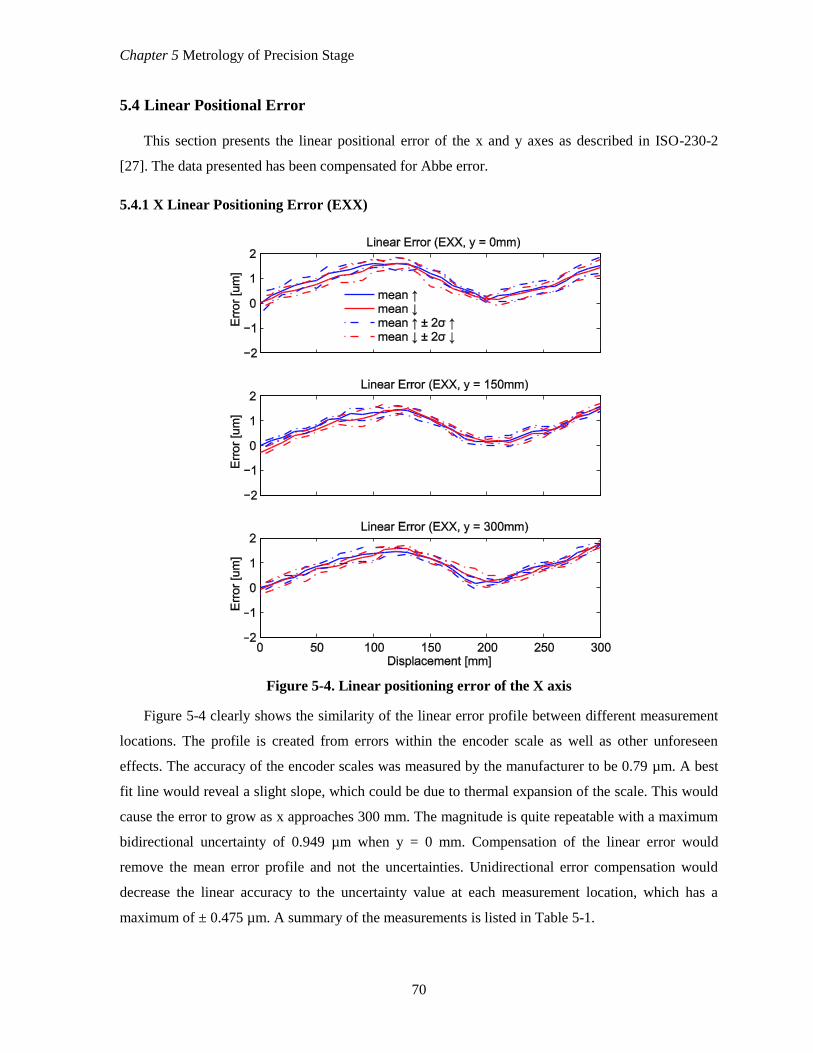
Chapter 5 Metrology of Precision Stage
70
5.4 Linear Positional Error
This section presents the linear positional error of the x and y axes as described in ISO-230-2
[27]. The data presented has been compensated for Abbe error.
5.4.1 X Linear Positioning Error (EXX)
Figure 5-4. Linear positioning error of the X axis
Figure 5-4 clearly shows the similarity of the linear error profile between different measurement
locations. The profile is created from errors within the encoder scale as well as other unforeseen
effects. The accuracy of the encoder scales was measured by the manufacturer to be 0.79 µm. A best
fit line would reveal a slight slope, which could be due to thermal expansion of the scale. This would
cause the error to grow as x approaches 300 mm. The magnitude is quite repeatable with a maximum
bidirectional uncertainty of 0.949 µm when y = 0 mm. Compensation of the linear error would
remove the mean error profile and not the uncertainties. Unidirectional error compensation would
decrease the linear accuracy to the uncertainty value at each measurement location, which has a
maximum of ± 0.475 µm. A summary of the measurements is listed in Table 5-1.

Chapter 5 Metrology of Precision Stage
71
Table 5-1. Metrology results for the X linear positioning error (w.r.t. table top)
Y = 0mm Unidirectional ↑ [µm] Unidirectional ↓ [µm] Bidirectional [µm]
Reversal value (𝐵) N/A N/A 0.234 (x = 60)
Mean reversal value (𝐵 ) N/A N/A 0.093
Range mean bidirectional positional
deviation (𝑀) N/A N/A 1.579
Systematic positional deviation (𝐸) 1.608 1.585 1.620
Repeatability of positioning (𝑅) 0.949 (x = 0) 0.812 (x = 150) 0.949
Accuracy (𝐴) 2.327 2.018 2.327
Y = 150mm Unidirectional ↑ [µm] Unidirectional ↓ [µm] Bidirectional [µm]
Reversal value (𝐵) N/A N/A 0.284 (x = 10)
Mean reversal value (𝐵 ) N/A N/A 0.046
Range mean bidirectional positional
deviation (𝑀) N/A N/A 1.666
Systematic positional deviation (𝐸) 1.472 1.859 1.859
Repeatability of positioning (𝑅) 0.514 (x = 100) 0.682 (x = 90) 0.750
Accuracy (𝐴) 1.737 2.105 2.105
Y = 300mm Unidirectional ↑ [µm] Unidirectional ↓ [µm] Bidirectional [µm]
Reversal value (𝐵) N/A N/A 0.253 (x = 70)
Mean reversal value (𝐵 ) N/A N/A 0.026
Range mean bidirectional positional
deviation (𝑀) N/A N/A 1.800
Systematic positional deviation (𝐸) 1.763 1.837 1.837
Repeatability of positioning (𝑅) 0.564 (x = 90) 0.658 (x = 190) 0.785
Accuracy (𝐴) 1.970 2.178 2.178
Figure 5-5 illustrates the error profiles in a 3-dimensional view with the error located at its
respected location within the machine’s work area.
Figure 5-5. Grid view of X axis linear positioning error

Chapter 5 Metrology of Precision Stage
72
5.4.2 Y Linear Positioning Error (EYY)
Figure 5-6. Linear positioning error of the Y axis
The profiles for each measurement in Figure 5-6 are similar. The profile shape is most likely due
to the error within the encoder scale itself. The maximum unidirectional accuracy is 3.04 µm, which
is mainly due to systematic deviation of the measurement. The maximum systematic positional
deviation is 2.61 µm, which can be removed through error compensation. However, with a maximum
uncertainty of 1.59 µm, error compensation methods will only provide a 2 times improvement. Table
5-2 summarizes the error data for each measurement location. It is expected that unidirectional error
compensation will reduce the linear positioning error to ±0.743 µm.

Chapter 5 Metrology of Precision Stage
73
Table 5-2. Metrology results for the Y linear positioning error (w.r.t. granite surface)
X = 0mm Unidirectional ↑
[µm]
Unidirectional ↓ [µm] Bidirectional [µm]
Reversal value (𝐵) N/A N/A 0.147 (y = 70)
Mean reversal value (𝐵 ) N/A N/A 0.012
Range mean bidirectional positional
deviation (𝑀) N/A N/A 2.280
Systematic positional deviation (𝐸) 2.217 2.366 2.366
Repeatability of positioning (𝑅) 0.703 (y = 10) 0.545 (y = 100) 0.703
Accuracy (𝐴) 2.516 2.726 2.726
X = 150mm Unidirectional ↑ [µm] Unidirectional ↓ [µm] Bidirectional
[µm]
Reversal value (𝐵) N/A N/A 0.662 (y = 70)
Mean reversal value (𝐵 ) N/A N/A 0.271
Range mean bidirectional positional
deviation (𝑀) N/A N/A 2.235
Systematic positional deviation (𝐸) 2.393 2.148 2.608
Repeatability of positioning (𝑅) 0.782 (y = 110) 0.581 (y = 140) 1.025
Accuracy (𝐴) 2.655 2.563 2.995
X = 300mm Unidirectional ↑ [µm] Unidirectional ↓ [µm] Bidirectional
[µm]
Reversal value (𝐵) N/A N/A 0.624 (y = 50)
Mean reversal value (𝐵 ) N/A N/A 0.265
Range mean bidirectional positional
deviation (𝑀) N/A N/A 2.246
Systematic positional deviation (𝐸) 2.251 2.258 2.448
Repeatability of positioning (𝑅) 1.486 (y = 0) 0.940 (y = 0) 1.593
Accuracy (𝐴) 2.756 2.805 3.040
Figure 5-7 illustrates the error profiles in a 3-dimensional view with the error located at its
respected location within the machine’s work area.
Figure 5-7. Grid view of Y axis linear positioning error

Chapter 5 Metrology of Precision Stage
74
5.5 Straightness Error (EYX, EZX, EXY, EZY)
This section presents the vertical and horizontal straightness error of the x and y axes. The data is
presented in accordance with ASME B5.54-2005 [25]. A least squares method is used to fit the data
to the reference straight line. The data is presented by determining the mean bidirectional maximum
and minimum and their corresponding uncertainties. It is displayed in this manner because the profile
is not usually of concern and rather the overall accuracy is the desired value. However, the profile is
required for compensation.
5.5.1 X Horizontal Straightness Error (EYX)
Figure 5-8. Horizontal straightness error of the X axis
The horizontal straightness is a direct correspondence to the gantry beam straightness. The
profiles are somewhat similar as the high points are located in the center of travel, but their overall
shapes do not correlate too closely. There are a couple factors which may contribute to the profile
differences, such as roll of the table (rotation about the x-axis) along its travel. This would be
categorized as Abbe error which cannot be adjusted, since roll was not measured. As well, it may be
due to the large y-axis pitch error. Different lateral loads may be applied on the table as it is located

Chapter 5 Metrology of Precision Stage
75
along the y-axis. The maximum systematic deviation is 0.94 µm with uncertainties of approximately
0.48 µm. The mean profiles for each measurement are used for error compensation, which should
improve the straightness error from 1.39 µm, to ±0.24 µm. Table 5-3 summarizes the error data for
each measurement location.
Table 5-3. Metrology results for the X horizontal straightness error
Y = 0mm Bidirectional [µm]
Systematic positional deviation (𝐸) 0.864
Repeatability of maximum (𝑅𝑚𝑎𝑥 ) 0.208
Repeatability of minimum (𝑅𝑚𝑖𝑛 ) 0.184
Accuracy (𝐴) 1.060
Y = 150mm Bidirectional [µm]
Systematic positional deviation (𝐸) 0.943
Repeatability of maximum (𝑅𝑚𝑎𝑥 ) 0.403
Repeatability of minimum (𝑅𝑚𝑖𝑛 ) 0.481
Accuracy (𝐴) 1.385
Y = 300mm Bidirectional [µm]
Systematic positional deviation (𝐸) 0.794
Repeatability of maximum (𝑅𝑚𝑎𝑥 ) 0.065
Repeatability of minimum (𝑅𝑚𝑖𝑛 ) 0.148
Accuracy (𝐴) 0.900
Figure 5-9 illustrates the error profiles in a 3-dimensional view with the error located at its
respected location within the machine’s work area.
Figure 5-9. Grid view of X axis horizontal straightness error

Chapter 5 Metrology of Precision Stage
76
5.5.2 X Vertical Straightness Error (EZX)
Figure 5-10. Vertical straightness error of the X axis
The vertical straightness of the x-axis is strongly influenced by the flatness profile of the granite
surface. The reason for different profiles in Figure 5-10 is that the table is travelling along different
sections of the granite, which have different flatness profiles. The maximum systematic deviation is
0.905 µm along the center of the granite surface. The maximum uncertainty is seen when y = 300 mm
and corresponds to the uncertainty of the minimum mean. Overall, error compensation should be able
to reduce the maximum accuracy from 1.08 µm, to ±0.17 µm. However, this will not be possible until
a vertical axis is installed over top of the stage. Table 5-4 summarizes the error data for each
measurement location.

Chapter 5 Metrology of Precision Stage
77
Table 5-4. Metrology results of the X vertical straightness error
Y = 0mm Bidirectional [µm]
Systematic positional deviation (𝐸) 0.822
Repeatability of maximum (𝑅𝑚𝑎𝑥 ) 0.096
Repeatability of minimum (𝑅𝑚𝑖𝑛 ) 0.081
Accuracy (𝐴) 0.911
Y = 150mm Bidirectional [µm]
Systematic positional deviation (𝐸) 0.905
Repeatability of maximum (𝑅𝑚𝑎𝑥 ) 0.185
Repeatability of minimum (𝑅𝑚𝑖𝑛 ) 0.162
Accuracy (𝐴) 1.079
Y = 300mm Bidirectional [µm]
Systematic positional deviation (𝐸) 0.544
Repeatability of maximum (𝑅𝑚𝑎𝑥 ) 0.097
Repeatability of minimum (𝑅𝑚𝑖𝑛 ) 0.342
Accuracy (𝐴) 0.763
Figure 5-11 illustrates the error profiles in a 3-dimensional view with the error located at its
respected location within the machine’s work area.
Figure 5-11. Grid view of X axis vertical straightness error

Chapter 5 Metrology of Precision Stage
78
5.5.3 Y Horizontal Straightness Error (EXY)
Figure 5-12. Horizontal straightness error of the Y axis
The horizontal straightness error corresponds to the straightness of the granite guideway. The
profiles of y = 150 mm and y = 300 mm are similar, but both differ from the first. This may be due to
roll of the table (rotation about the y-axis) as the table travels. As explained earlier, this is Abbe error
which is not removed from the data, since roll was not measured. The maximum uncertainty of the
data is 0.091 µm, with a maximum systematic deviation of 1.44 µm. Since the uncertainty is low,
error compensation is more effective as it will reduce the error substantially, to ±0.045 µm. Table 5-5
summarizes the error at each measurement location.
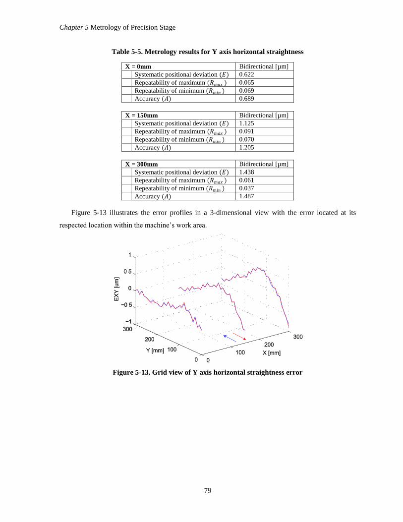
Chapter 5 Metrology of Precision Stage
79
Table 5-5. Metrology results for Y axis horizontal straightness
X = 0mm Bidirectional [µm]
Systematic positional deviation (𝐸) 0.622
Repeatability of maximum (𝑅𝑚𝑎𝑥 ) 0.065
Repeatability of minimum (𝑅𝑚𝑖𝑛 ) 0.069
Accuracy (𝐴) 0.689
X = 150mm Bidirectional [µm]
Systematic positional deviation (𝐸) 1.125
Repeatability of maximum (𝑅𝑚𝑎𝑥 ) 0.091
Repeatability of minimum (𝑅𝑚𝑖𝑛 ) 0.070
Accuracy (𝐴) 1.205
X = 300mm Bidirectional [µm]
Systematic positional deviation (𝐸) 1.438
Repeatability of maximum (𝑅𝑚𝑎𝑥 ) 0.061
Repeatability of minimum (𝑅𝑚𝑖𝑛 ) 0.037
Accuracy (𝐴) 1.487
Figure 5-13 illustrates the error profiles in a 3-dimensional view with the error located at its
respected location within the machine’s work area.
Figure 5-13. Grid view of Y axis horizontal straightness error

Chapter 5 Metrology of Precision Stage
80
5.5.4 Y Vertical Straightness Error (EZY)
Figure 5-14. Vertical straightness error of the Y axis
The largest amount of linear error of the machine is the vertical straightness of the y-axis,
displayed in Figure 5-14. The error is related to the flatness of the granite surface. Even though the
errors may be large, the uncertainties are low, which allows for large improvements by error
compensation. The maximum uncertainty is 0.149 µm, which occurs at the maximum mean when x =
0 mm. The maximum systematic deviation is 3.253 µm when x = 300 mm. Error compensation is
expected to improve the accuracy from 3.37 µm, to ±0.075 µm.
Some Abbe error is present is the data shown in Figure 5-14 for the measurements located at x =
0, 300. Since the optics were located at the edge of the worktable, roll will contribute to a vertical
displacement. Roll measurements must be completed prior to implementing the compensation
algorithms.

Chapter 5 Metrology of Precision Stage
81
Table 5-6. Metrology results for Y axis vertical straightness
X = 0mm Bidirectional [µm]
Systematic positional deviation (𝐸) 2.387
Repeatability of maximum (𝑅𝑚𝑎𝑥 ) 0.149
Repeatability of minimum (𝑅𝑚𝑖𝑛 ) 0.053
Accuracy (𝐴) 2.488
X = 150mm Bidirectional [µm]
Systematic positional deviation (𝐸) 2.409
Repeatability of maximum (𝑅𝑚𝑎𝑥 ) 0.107
Repeatability of minimum (𝑅𝑚𝑖𝑛 ) 0.095
Accuracy (𝐴) 2.510
X = 300mm Bidirectional [µm]
Systematic positional deviation (𝐸) 3.253
Repeatability of maximum (𝑅𝑚𝑎𝑥 ) 0.109
Repeatability of minimum (𝑅𝑚𝑖𝑛 ) 0.128
Accuracy (𝐴) 3.371
Figure 5-15 illustrates the error profiles in a 3-dimensional view with the error located at its
respected location within the machine’s work area.
Figure 5-15. Grid view of Y axis vertical straightness error

Chapter 5 Metrology of Precision Stage
82
5.6 Angular Error (EBX, ECX, EAY, ECY)
This section presents the angular errors of the x and y axes. The data is presented in the same
manner as ISO-230-2 [39]. Abbe error is not present in angular measurements, as the rotation of an
object is identical at any measurement location.
5.6.1 X Pitch Error (EBX)
Figure 5-16. Pitch error of the X axis
Figure 5-16 displays the pitch error of the x-axis at each measurement location. Pitch error is the
resultant of the curvature of the guideways, which in this case is the curvature of the top granite
surface. The data presented is the relative angular, error since the initial absolute angular error is
unknown. The maximum bidirectional systematic deviation occurs when y = 150 mm, which is 8.77
µm/m with an uncertainty of 5 µm/m for a total accuracy of 12.0 µm/m. Compensation of angular
errors requires two orthogonal rotation axes, which in this case will be present when the trunnion is
installed. It is expected to reduce the angular error from 12.0 µm/m to ±3.71 µm/m.

Chapter 5 Metrology of Precision Stage
83
Table 5-7. Metrology results for the X pitch error
Y = 0mm Unidirectional ↑
[µm/m]
Unidirectional ↓
[µm/m]
Bidirectional
[µm/m]
Reversal value (𝐵) N/A N/A 1.32 (x = 0)
Mean reversal value (𝐵 ) N/A N/A -0.126
Range mean bidirectional positional
deviation (𝑀) N/A N/A 2.37
Systematic positional deviation (𝐸) 1.91 2.88 2.88
Repeatability of positioning (𝑅) 6.50 (x = 270) 6.76 (x = 10) 7.42
Accuracy (𝐴) 7.80 8.46 8.46
Y = 150mm Unidirectional ↑
[µm/m]
Unidirectional ↓
[µm/m]
Bidirectional
[µm/m]
Reversal value (𝐵) N/A N/A 1.28 (x = 250)
Mean reversal value (𝐵 ) N/A N/A -0.081
Range mean bidirectional positional
deviation (𝑀) N/A N/A 7.93
Systematic positional deviation (𝐸) 7.93 8.77 8.77
Repeatability of positioning (𝑅) 5.74 (x = 50) 5.11 (x = 210) 5.00
Accuracy (𝐴) 12.0 11.3 12.0
Y = 300mm Unidirectional ↑
[µm/m]
Unidirectional ↓
[µm/m]
Bidirectional
[µm/m]
Reversal value (𝐵) N/A N/A 1.66 (x = 280)
Mean reversal value (𝐵 ) N/A N/A -0.314
Range mean bidirectional positional
deviation (𝑀) N/A N/A 4.23
Systematic positional deviation (𝐸) 4.47 4.70 4.70
Repeatability of positioning (𝑅) 4.40 (x = 300) 4.49 (x = 100) 5.39
Accuracy (𝐴) 7.95 7.78 8.47
Figure 5-17 illustrates the error profiles in a 3-dimensional view with the error located at its
respected location within the machine’s work area.
Figure 5-17. Grid view of X axis pitch error

Chapter 5 Metrology of Precision Stage
84
5.6.2 X Yaw Error (ECX)
Figure 5-18. Yaw error of the X axis
Figure 5-18 displays the yaw error of the x-axis. This error is mainly created by the curvature of
the gantry beam. The data collected at y = 150 has significantly larger uncertainty, however the mean
value is similar to the other locations. Occasionally, laser misalignment will result in additional pulses
within the electronics of the metrology equipment. This can lead to the data drifting during
measurements, leading to larger uncertainties. This is assumed to have occurred while measuring the
x-axis yaw error at y = 150 mm. The uncertainty levels for this test will not be considered for the
predicted improvement with geometric compensation. The maximum bidirectional systematic
deviation is 14.4 µm/m, while the maximum bidirectional uncertainty is 3.83 µm/m. Therefore, it can
be assumed that error compensation will remove the systematic deviation and reduce the accuracy
from 15.3 µm/m to ±1.92 µm/m.

Chapter 5 Metrology of Precision Stage
85
Table 5-8. Metrology results for the X yaw error
Y = 0mm Unidirectional ↑
[µm/m]
Unidirectional ↓
[µm/m]
Bidirectional
[µm/m]
Reversal value (𝐵) N/A N/A 0.784 (x = 210)
Mean reversal value (𝐵 ) N/A N/A -0.046
Range mean bidirectional positional
deviation (𝑀) N/A N/A 12.6
Systematic positional deviation (𝐸) 12.3 12.9 12.9
Repeatability of positioning (𝑅) 2.85 (x = 70) 3.04 (x = 130) 2.99
Accuracy (𝐴) 13.5 14.4 14.4
Y = 150mm Unidirectional ↑
[µm/m]
Unidirectional ↓
[µm/m]
Bidirectional
[µm/m]
Reversal value (𝐵) N/A N/A 1.65 (x = 10)
Mean reversal value (𝐵 ) N/A N/A -0.689
Range mean bidirectional positional
deviation (𝑀) N/A N/A 13.7
Systematic positional deviation (𝐸) 13.3 14.2 14.4
Repeatability of positioning (𝑅) 11.3 (x = 60) 8.36 (x = 130) 10.1
Accuracy (𝐴) 23.1 21.4 23.1
Y = 300mm Unidirectional ↑
[µm/m]
Unidirectional ↓
[µm/m]
Bidirectional
[µm/m]
Reversal value (𝐵) N/A N/A 0.675 (x = 210)
Mean reversal value (𝐵 ) N/A N/A -0.066
Range mean bidirectional positional
deviation (𝑀) N/A N/A 14.0
Systematic positional deviation (𝐸) 14.0 14.0 14.2
Repeatability of positioning (𝑅) 2.89 (x = 270) 3.45 (x = 270) 3.83
Accuracy (𝐴) 15.2 15.3 15.3
Figure 5-19 illustrates the error profiles in a 3-dimensional view with the error located at its
respected location within the machine’s work area.
Figure 5-19. Grid view of X yaw error

Chapter 5 Metrology of Precision Stage
86
5.6.3 Y Pitch Error (EAY)
Figure 5-20. Pitch error of the Y axis
The y-axis pitch error is the largest angular error of the machine. With a maximum bidirectional
systematic deviation of 70.9 µm/m, it is significantly higher than the other angular errors. The
uncertainty, however, is of the same order as the other angular errors with a maximum bidirectional
uncertainty of 6.83 µm/m. This error is due to the curvature of the granite surface, which can be seen
in Figure 5-14. The accuracy of the pitch error is expected to improve from 76.5 µm/m to ±3.92
µm/m, after compensation.

Chapter 5 Metrology of Precision Stage
87
Table 5-9. Metrology results for the Y pitch error
X = 0mm Unidirectional ↑
[µm/m]
Unidirectional ↓
[µm/m]
Bidirectional
[µm/m]
Reversal value (𝐵) N/A N/A 0.524 (y = 10)
Mean reversal value (𝐵 ) N/A N/A -0.113
Range mean bidirectional positional
deviation (𝑀) N/A N/A 70.7
Systematic positional deviation (𝐸) 70.5 70.8 70.9
Repeatability of positioning (𝑅) 6.96 (y = 10) 7.30 (y = 30) 6.83
Accuracy (𝐴) 76.5 75.7 76.5
X = 150mm Unidirectional ↑
[µm/m]
Unidirectional ↓
[µm/m]
Bidirectional
[µm/m]
Reversal value (𝐵) N/A N/A 0.662 (y = 30)
Mean reversal value (𝐵 ) N/A N/A -0.185
Range mean bidirectional positional
deviation (𝑀) N/A N/A 67.1
Systematic positional deviation (𝐸) 67.0 67.3 67.5
Repeatability of positioning (𝑅) 7.30 (y = 140) 5.91 (y = 190) 6.57
Accuracy (𝐴) 72.9 72.4 72.9
X = 300mm Unidirectional ↑
[µm/m]
Unidirectional ↓
[µm/m]
Bidirectional
[µm/m]
Reversal value (𝐵) N/A N/A 0.971 (y = 60)
Mean reversal value (𝐵 ) N/A N/A 0.551
Range mean bidirectional positional
deviation (𝑀) N/A N/A 62.8
Systematic positional deviation (𝐸) 63.0 62.6 63.1
Repeatability of positioning (𝑅) 6.08 (y = 80) 5.93 (y = 280) 6.25
Accuracy (𝐴) 68.0 65.9 68.0
Figure 5-21 illustrates the error profiles in a 3-dimensional view with the error located at its
respected location within the machine’s work area.
Figure 5-21. Grid view of Y pitch error

Chapter 5 Metrology of Precision Stage
88
5.6.4 Y Yaw Error (ECY)
Figure 5-22. Yaw error of the Y axis
The yaw error of the y axis is the smallest angular error of the machine. This error is from the
curvature of the granite guideway. This error is smaller than the other angular errors, due to the four
preloaded air bearings of the gantry spanning a large distance. Since their separation is large, the
angular error is small. The maximum bidirectional systematic deviation is 2.49 µm/m with a
maximum uncertainty of 4.73 µm/m. The y-axis yaw error cannot be improved by a very significant
amount since its uncertainty is larger than the mean deviation. The expected accuracy improvement
after error compensation is from 5.35 µm/m to ±2.37 µm/m.

Chapter 5 Metrology of Precision Stage
89
Table 5-10. Metrology results for the Y yaw error
X = 0mm Unidirectional ↑
[µm/m]
Unidirectional ↓
[µm/m]
Bidirectional
[µm/m]
Reversal value (𝐵) N/A N/A 0.850 (y = 50)
Mean reversal value (𝐵 ) N/A N/A -0.424
Range mean bidirectional positional
deviation (𝑀) N/A N/A 2.20
Systematic positional deviation (𝐸) 1.95 2.48 2.48
Repeatability of positioning (𝑅) 2.36 (y = 250) 2.06 (y = 100) 2.28
Accuracy (𝐴) 3.21 3.94 3.94
X = 150mm Unidirectional ↑
[µm/m]
Unidirectional ↓
[µm/m]
Bidirectional
[µm/m]
Reversal value (𝐵) N/A N/A 0.1.63 (y = 50)
Mean reversal value (𝐵 ) N/A N/A -0.756
Range mean bidirectional positional
deviation (𝑀) N/A N/A 1.74
Systematic positional deviation (𝐸) 1.27 2.41 2.41
Repeatability of positioning (𝑅) 4.03 (y = 20) 4.75 (y = 290) 4.73
Accuracy (𝐴) 4.74 5.35 5.35
X = 300mm Unidirectional ↑
[µm/m]
Unidirectional ↓
[µm/m]
Bidirectional
[µm/m]
Reversal value (𝐵) N/A N/A 0.973 (y = 50)
Mean reversal value (𝐵 ) N/A N/A -0.437
Range mean bidirectional positional
deviation (𝑀) N/A N/A 2.27
Systematic positional deviation (𝐸) 2.12 2.43 2.49
Repeatability of positioning (𝑅) 1.57 (y = 10) 1.79 (y = 180) 2.09
Accuracy (𝐴) 3.28 3.14 3.29
Figure 5-23 illustrates the error profiles in a 3-dimensional view with the error located at its
respected location within the machine’s work area.
Figure 5-23. Grid view of Y yaw error

Chapter 5 Metrology of Precision Stage
90
5.7 Conclusion
This chapter has presented the data and analysis of metrology measurements of the precision
stage. Linear positioning error, vertical and horizontal straightness, as well as pitch and yaw errors
were measured using a laser interferometer and presented in accordance with international metrology
standards. Table 5-11 summarizes the maximum accuracies of all measurement locations for each test
performed.
Table 5-11. Summary of accuracies from error measurements
Error Units
X-Axis
Linear Positioning 2.327 µm
Horizontal Straightness 1.385 µm
Vertical Straightness 1.079 µm
Pitch 12.0 µm/m
Yaw 23.1 µm/m
Y-Axis
Linear Positioning 3.040 µm
Horizontal Straightness 1.487 µm
Vertical Straightness 3.371 µm
Pitch 76.5 µm/m
Yaw 5.35 µm/m
Geometric error compensation will be used in future experiments to improve the accuracy of the
machine. It is assumed that mean error values will be compensated, leaving the uncertainty as the
remaining error. Table 5-12 lists the estimated errors with compensation applied.
Table 5-12. Summary of predicted accuracies assuming geometric error compensation
Error Units
X-Axis
Linear Positioning 0.475 µm
Horizontal Straightness 0.241 µm
Vertical Straightness 0.063 µm
Pitch 2.87 µm/m
Yaw 1.73 µm/m
Y-Axis
Linear Positioning 0.743 µm
Horizontal Straightness 0.031 µm
Vertical Straightness 0.064 µm
Pitch 3.65 µm/m
Yaw 2.38 µm/m

91
Chapter 6
Conclusions and Future Work
This thesis has presented the mechanical design, controller design and metrology of a novel ultra-
precision planar stage intended as a base for a 5-axis machine tool. Its workspace of 300x300 mm2
provides macro and micro operational capabilities for many applications.
The design of the machine incorporated a T-type gantry and worktable configuration with an
asymmetric granite guideway to provide a majority of the machine’s yaw and lateral stiffness. The
gantry beam extends over the workspace to act as a guideway for the worktable. Rigid body yaw
vibration of the gantry was observed at ~ 68 Hz due to its high moment of inertia around the y-axis
guideway. A secondary motor for the gantry was installed at the end, to actively stiffen the structure
and dampen the vibration mode. To further stiffen the structure, the gantry beam and worktable were
decoupled from vertical loads, by installing a Vacuum Pre-Loaded (VPL) air bearing underneath the
worktable to support its load on the granite surface. Hence, vertical deflections of the beam do not
result in position deviations on the worktable surface. As well, the VPL provides higher vertical and
pitch stiffness than aerostatic bearings, which was confirmed experimentally. Direct drive linear
motors were implemented to actuate the stage up to 10 m/s2 acceleration and 1 m/s velocity. Their
non-contact and direct drive properties resulted in higher servo performance and positional accuracy
than traditional mechanical systems, like ball-screw drives.
Liquid cooled motor couplings were designed to mitigate heat generated by the linear motors
during high transient operations. Finite element analyses of the x- and y-axis coupling designs
demonstrated their capabilities to maintain a constant 20°C temperature on the surface in contact with
the stage. The control of the laboratory temperature revealed a ±1°C range, which was found to be too
high. Further improvements to the thermostat controller are expected to lower the range to ±0.2°C.
Static stiffness testing of the stage revealed a discrepancy between theoretical and experimental
stiffness values. It was determined that the pitch stiffness of the VPL, and its bolted interface, resulted
in lower values when a lateral load was applied on the top surface of the worktable. Also, other
bearings are still under point contact allowing for relative motion between the bearing and guideways.
The resulting lateral stiffness values when loaded at the top of the worktable were 22.2 N/µm in the
x-axis and 23.9 N/µm in the y-axis. These stiffness values are expected to improve after cementing
the bearings.
Dynamic testing of the drive systems using Frequency Response Function (FRF) measurements
revealed the vibration modes of the stage structure. The first mode present in the x-axis occurs at 220

Chapter 6 Conclusions and Future Work
92
Hz and is believed to be due to the pitching of the worktable. A prominent mode at ~68 Hz in the y-
axis is due to the rigid body yaw vibration about the four preloaded air bearings for the gantry. A
second mode in the y-axis occurs between 320 Hz and 364 Hz, and is considered to be due to the
bending mode of the beam. This mode is dependent on the position of the x-axis. Model parameters
were identified through least squares parameter estimation of the experimental FRF tests. A loop
shaping controller was designed for the x-axis with a crossover frequency of 100 Hz and phase
margin of 25°. The resulting maximum sensitivity of the loop function was 2.6 at approximately 100
Hz, which is slightly aggressive, but favors better tracking results. A multivariable control framework
was implemented for the y-axis due to the strong coupling in the dual actuator design of the gantry.
Signal averaging of the encoder measurements was used to determine the position of the center of
mass of the stage. The averaging technique negated the 68 Hz mode, allowing for higher controller
bandwidth designs and better tracking response. As well, active damping High (200 mm/s) and low
(20 mm/s) speed tracking results were completed to test the controller designs. Peak errors of 1.61 µm
and 1.45 µm for the x- and y-axes respectively, were measured for the low speed tracking. The high
speed test measured peak errors of 2.74 µm and 2.41 µm for the x- and y-axes respectively.
Static errors of the machine were measured using laser interferometry for both axes. Linear
positioning, straightness and angular errors were measured at 10 mm increments over the full range of
motion. A final error budget, Table 6-1, includes updated values of geometric, dynamic, servo and
thermal errors of the machine.
Suggestions for future work include improvement to the environmental temperature control of the
laboratory. Application of cement around the bearings, especially the VPL, should further improve
the stiffness of the structure and also the control bandwidth and accuracy. Some ideas learned through
the course of research are as follows:
Redesign machines base structure to avoid excitation of base vibrations, which reduce
positioning accuracy.
Lower the profile of the stage structure to improve pitch stiffness.
Align actuators with center of mass to reduce moment loads during acceleration.
Locate encoders closer to work area to minimize position feedback errors.
Implement linear amplifiers to replace PWM amplifier.
Investigate stiffness features of VPL to develop analytical model.
Apply VPL technology to the gantry to increase its pitch stiffness

Chapter 6 Conclusions and Future Work
93
Table 6-1. Final Error Budget
Error Magnitude (nm)
Without Compensation With Compensation1
X Y Z X Y Z
Linear 2327 3040 - 475 743 -
Straightness
Horizontal 1487 1385 - 31 241 -
Vertical2 - - 3371 - - 64
Angular (included in Linear) 0 0 0 0 0 0
Dynamic (0.2 g acceleration) 2845 2960 0 427 444 0
Servo (@ 0.2 g acc., 50 m/s3 jerk) 2740 2410 - 2740 2410 -
Thermal
Friction 0 0 0 0 0 0
Drive System 0 0 0 0 0 0
Environment (20 ± 0.2°C) 1520 270 0 1520 270 0
Static Error
Arithmetic Sum (EA) 5334 4695 3371 2026 1254 64
RMS3 Sum (ER) 1820 1935 3371 920 477 64
Mean ((EA + ER)/2) 3577 3315 3371 1473 866 64
Maximum Resultant Error ET = 5.93 µm ET = 1.71 µm
Static + Dynamic Error
Arithmetic Sum (EA) 10919 10065 3371 5193 4108 64
RMS3 Sum (ER) 2260 2272 3371 1430 1157 64
Mean ((EA + ER)/2) 6590 6168 3371 3312 2632 64
Maximum Resultant Error ET = 9.64 µm ET = 4.23 µm
1 Compensation indicates the correction of repeatable geometric & dynamic errors by shifting the position
commands. 15% uncertainty in dynamic error compensation is assumed. 2 Maximum of both axes.
3 Assumes normal probability for each error about its mean value.

94
References
[1] Slocum, A. H., 1992, Precision Machine Design, Society of Manufacturing Engineers, Dearborn
MI.
[2] Shinno, H., Yoshioka, H., Taniguchi, K., 2007, A Newly Developed Linear Motor-Driven
Aerostatic X-Y Planar Motion Table System for Nano-Machining, Annals of the CIRP,
56/1:369-372
[3] Shinno, H., Hashizume, H., 1999, Nanometer Positioning of a Linear Motor-Driven
Ultraprecision Aerostatic Table System with Electrorheological Fluid Dampers, Annals of the
CIRP, 48/1:289-292
[4] Cheng, X., Nakamoto, K., Sugai, M., Matsumoto, S., Wang, Z.G., Yamazaki, K., 2008,
Development of ultra-precision machining system with unique wire EDM tool fabrication
system for micro/nano-machining, Annals of the CIRP, 57/1:415-420
[5] Holmes, M., Trumpet, D., Hocken, R., 1995, Atomic-Scale Precision Motion Control Stage
(The Angstrom Stage), Annals of the CIRP, 44/1:455-460
[6] Aerotech Inc., 2010, ABL9000 Air Bearing Stage, Retrieved January 11, 2010, from the
Aerotech web site, http://www.aerotech.com/products/airbearing/abl9000.html
[7] Precitech, Inc. 2010, Nanoform 700 Ultra, Retrieved January 11, 2010, from Precitech web site,
http://www.precitech.com/Precitech_nano700_features.html
[8] Moore Tool Company, 2010, Drum Lathes – Machines for development and production of
microstructured surfaces, Retrieved January 11, 2010, from Moore Tool website,
http://www.mooretool.com/PDF%20Brochures/Drum%20Lathes.pdf
[9] ASML, 2010, Twinscan NXT:1950i: 193-nm Step-and-Scan, Retrieved from ASML web site,
http://www.asml.com/asml/show.do?ctx=6720&rid=36951
[10] Schwenke, H., Knapp, W., Haitjema, H., Weckenmann, A., Schmitt, R., Delbressine, F., 2008,
Geometric error measurement and compensation of machines – An Update, Annals of the CIRP,
57/2:660-675
[11] Kamalzadeh, A., 2008, Ph.D. Thesis: Precision Control of High Speed Ball Screw Drives. The
University of Waterloo, Waterloo, Canada.
[12] Sriyotha, P., Nakamoto, K., Sugai, M., Yamazaki, K., 2006, Development of 5-Axis Linear
Motor Driven Super-Precision Machine, Annals of the CIRP, 55/1:381-384
[13] ETEL S.A., 2010, Linear Motors Overview, Retrieved January 11, 2010, from ETEL web site,
http://www.etel.ch/linear_motors
[14] Donmez, A., 1985, Ph.D. Thesis: A General Methodology for Machine Tool Accuracy
Enhancement: Theory, Application and Implementation. Purdue University, West Lafayette,
Indiana.
[15] Automation Creations Inc., 2010, Online Materials Information Resource, Retrieved, January
11, 2010, from website, http://www.matweb.com
[16] ETEL S.A., 2010, Torque Motors, Retrieved January 11, 2010, from ETEL web site,
http://www.etel.ch/torque_motors

References
95
[17] Erkorkmaz, K., 2007, Course notes: Precision Control Theory, University of Waterloo,
Waterloo, Canada.
[18] Tackeuchi, Y., Sakaida, Y., Sawada, K., Sata, T., 2000, Development of a 5-Axis Control
Ultraprecision Milling Machine for Micromachining Based on Non-Friction Servomechanisms,
Annals of CIRP, 49/1:295-298.
[19] New Way Air Bearings, 2010, Vacuum Preloaded Air Bearings, Retrieved January 2010, from
website, http://www.newwayairbearings.com/Vacuum-Preloaded-Air-Bearings
[20] Shinno, H., Hashizume, H., Yoshioka, H., Komatsu, K., Shinshi, T., Sato, K., 2004, X-Y-Θ
Nano-Positioning Table System for a Mother Machine, Annals of the CIRP, 53/1:337-340.
[21] Cortesi, R., 2000, M.Sc. Thesis: An Easy to Manufacture Non-Contact Precision Linear Motion
System and its Applications. Massachusetts Institute of Technology, Boston, Massachusetts.
[22] ITP Group, 2010, Reconditioned and Pre-Owned Coordinate Measuring Machines, Retrieved
January 11, 2010, from ITP group web site,
http://www.itpgroup.co.uk/products/reconditioned_cmms/reconditioned_cmms.html
[23] Moylan, S., July 2009, Private communication, National Institute of Standards and Technology.
[24] ISO-230-1:1996, Test Code for Machine Tools, Part 1: Geometric Accuracy of Machines
Operating Under No-load or Quasi-Static Conditions, ISO, Geneva.
[25] ASME B5.54-2005, Methods for Performance Evaluation of Computer Numerically Controlled
Machining Centers.
[26] Stone, J.A., Zimmerman, J.H., 2010, Index of Refraction of Air, Retrieved January 10, 2010,
from NIST website, http://emtoolbox.nist.gov/Wavelength/Documentation.asp
[27] ISO 230-6:2002, Test code for machine tools, Part 6: Determination of Positioning Accuracy on
Body and Face Diagonals (Diagonal Displacement Tests), ISO, Geneva.
[28] New Way Air Bearings, 2006, Air Bearing Application and Design Guide, Retrieved January
10, 2010, from New Way Air Bearing web site: http://www.newwayairbearings.com/Detailed-
Product-Information
[29] Devitt Machinery Company, 2010, Moglice: Moldable Bearing Material, Retrieved, January 11,
2010, from website, http://www.moglice.com
[30] New Way Air Bearings, 2010, Product Line Comparison: Flat Round Air Bearings, Retrieved
January 10, 2010, from New Way Air Bearing web site: http://www.newwayairbearings.com
[31] ETEL S.A., 2010, Ironless Linear Motor: ILM06-060, Retrieved January 11, 2010, from ETEL
web site, http://www.etel.ch/documents/showFile.asp?ID=2005
[32] Vierck, R.K., 1979, Vibration Analysis (2nd Edition), Harper & Row.
[33] Banks, C., 2007, Fourth year design report, High Precision Linear Motor Coupling, University
of Waterloo, Waterloo, Canada
[34] Thompson, D.C., 1989, The Design of an Ultra-Precision CNC Measuring Machine, Annals of
the CIRP, 38/1:501-504
[35] Okwudire, C., Ph.D. Thesis: Modeling and Control of High Speed Machine Tool Feed Drives.
University of British Columbia, Vancouver, Canada.
[36] Franklin, G., Powell, J.D., Emami-Naeini, A., 2005, Feedback Control of Dynamic Systems,
(5th Edition), Prentice Hall.

References
96
[37] Weng, M.-C., Lu, X., Trumper, D.L., 2002, Vibration Control of Flexible Beams using Sensor
Averaging and Actuator Averaging Methods. IEEE, Trans. On Control Systems Technology,
10/4:568-577.
[38] Skogestad, S., Postlethwaite, I., 2005, Multivariable Feedback Control – Analysis and Design
(2nd Edition), Wiley.
[39] ISO 230-2:2006, Test Code for Machine Tools. Part 2. Determination of Accuracy and
Repeatability of Positioning of Numerically Controlled Axes, ISO, Geneva


![Welcome! []Examples of matching xy xy anywhere in string ^xy xy at beginning of string xy$ xy at end of string ^xy$ string that contains only xy ^ matches any string, even empty ^$](https://img.dokumen.tips/doc/110x75/60836582b1fa9828ec278d05/welcome-examples-of-matching-xy-xy-anywhere-in-string-xy-xy-at-beginning-of.jpg)


![수치해석 (Numerical Analysis] · 2019. 8. 29. · 법 칙 (rule) 자연 ... xyy 2 xxxxy 6543 2 xyxyxyxyxy xy xy xy xy xy yxyyxyyxyy 65432 22 3 23 4 24 5623456 ... 근한 결과를](https://img.dokumen.tips/doc/110x75/6094b2bc38b4a6116148a9c8/-numerical-analysis-2019-8-29-e-rule-xyy-2.jpg)


