Embed Size (px)
Citation preview

DESIGN AND FPGA IMPLEMENTATION OF AN EFFICIENT
DEINTERLEAVING ALGORITHM
A THESIS SUBMITTED TO THE GRADUATE SCHOOL OF NATURAL AND APPLIED SCIENCES
OF MIDDLE EAST TECHNICAL UNIVERSITY
BY
MUHAMMET ERTUĞ OLGUN
IN PARTIAL FULFILLMENT OF THE REQUIREMENTS FOR
THE DEGREE OF MASTER OF SCIENCE IN
ELECTRICAL AND ELECTRONICS ENGINEERING
AUGUST 2008

Approval of the thesis:
DESIGN AND FPGA IMPLEMENTATION OF AN EFFICIENT
DEINTERLEAVING ALGORITHM
submitted by MUHAMMET ERTUĞ OLGUN in partial fulfillment of the requirements for the degree of Master of Science in Electrical and Electronics
Engineering Department, Middle East Technical University by,
Prof. Dr. Canan Özgen ___________ Dean, Graduate School of Natural and Applied Sciences Prof. Dr. İsmet ERKMEN ___________ Head of Department, Electrical and Electronics Engineering Prof. Dr. Gözde Akar Bozdağı ___________ Supervisor, Electrical and Electronics Engineering Dept., METU
Assoc. Prof. Dr. Sencer Koç ___________ Co supervisor, Electrical and Electronics Engineering Dept., METU
Examining Committee Members :
Prof. Dr. Fatih Canatan ____________ Electrical and Electronics Engineering Dept., METU Prof. Dr. Gözde Bozdağı Akar ____________ Electrical and Electronics Engineering Dept., METU Assoc. Prof. Dr. Sencer Koç ____________ Electrical and Electronics Engineering Dept., METU Assist. Prof. Dr. Çağatay Candan ____________ Electrical and Electronics Engineering Dept., METU M.S. Oral Dinçer ____________ Chief Engineer, METEKSAN
Date: 15.08.2008__

iii
I hereby declare that all information in this document has been obtained and
presented in accordance with academic rules and ethical conduct. I also declare
that, as required by these rules and conduct, I have fully cited and referenced
all material and results that are not original to this work.
Name, Last name : Muhammet Ertuğ OLGUN
Signature :

iv
ABSTRACT
DESIGN AND FPGA IMPLEMENTATION OF AN EFFICIENT DEINTERLEAVING ALGORITHM
OLGUN, Muhammet Ertuğ
M.S., Department of Electrical and Electronics Engineering
Supervisor : Prof. Dr. Gözde Bozdağı Akar
Co Supervisor : Assoc. Prof. Dr. Sencer Koç
August 2008, 73 pages
In this work, a new deinterleaving algorithm that can be used as a part of an ESM
system and its implementation by using an FPGA is studied. The function of the
implemented algorithm is interpreting the complex electromagnetic military field in
order to detect and determine different RADARs and their types by using incoming
RADAR pulses and their PDWs. It is assumed that RADAR signals in the space are
received clearly and PDW of each pulse is generated as an input to the implemented
algorithm system. Clustering analysis and a new interpreting process is used to
deinterleave the RADAR pulses. In order to implement the algorithm, FPGA is used
for achieving a faster and more efficient system. Comparison of the new algorithm
and the previous deinterleaving studies is done. The simulation results are shown and
discussed in detail.
Keywords: Deinterleaving of RADAR pulses, Clustering, ESM, PDW, FPGA

v
ÖZ
VERİMLİ AYRIŞTIRMA ALGORİTMASININ TASARIMI VE FPGA UYGULAMASI
OLGUN, Muhammet Ertuğ
Yüksek Lisans, Elektrik ve Elektronik Mühendisliği Bölümü
Tez Yöneticisi : Prof. Dr. Gözde Akar Bozdağı
Ortak Tez Yöneticisi: Doç. Dr. Sencer Koç
Ağustos 2008, 73 sayfa
Bu tez çalışmasında, Elektronik Destek sistemlerinde kullanılabilecek yeni bir
ayrıştırma algoritması ve algoritmanın FPGA uygulaması çalışılmıştır. Uygulanmış
algoritmanın işlevi; farklı radarların ve çeşitlerinin, algılanan radar darbeleri ve
bunların darbe tanımlayıcı kelimelerini kullanarak, tespiti ve tayini için karmaşık
askeri elektromanyetik ortamların yorumlanmasıdır. Havadaki radar sinyalleri temiz
bir şekilde alınmış ve her darbenin darbe tanımlayıcı kelimelerinin uygulanmış
sisteme girdi olarak üretilmiş olduğu varsayılmıştır. Radar darbelerinin ayrıştırılması
için gruplama analizi ve yeni bir yorumlama işlemi kullanılmıştır. Daha hızlı ve
verimli bir sisteme ulaşmak için algoritmanın uygulamasında FPGA kullanılmıştır.
Yeni algoritma ile daha önceki ayrıştırma çalışmalarının karşılaştırması yapılmıştır.
Gerçekleme sonuçları gösterilmiş ve detaylı bir şekilde tartışılmıştır.
Anahtar Kelimeler: RADAR darbelerini ayrıştırma, Gruplama, Elektronik Destek Ölçümleri, Darbe Tanımlayıcı Kelime, FPGA

vi
To My Love, Başak

vii
ACKNOWLEDGMENTS
I would like to thank Prof. Dr. Gözde Bozdağı Akar for her valuable supervision and
also to Assoc. Prof. Dr. Sencer Koç for his support and tolerance throughout the
development and improvement of this thesis.
I am grateful to Oral Dinçer for his valuable decisions throughout the development of
this thesis. I am also grateful to Aselsan Electronics Industries Inc. and TUBITAK
for the resources and facilities that I used throughout thesis.
Thanks a lot to all my friends, especially Abdullah Volkan İpek, for their great
encouragement and their valuable help to accomplish this work.
Lastly, I would like to thank my parents, sisters and extended family for bringing up
and trusting in me, and Başak Eşlik, for giving me the strength and courage to finish
this work.

viii
TABLE OF CONTENTS
ABSTRACT................................................................................................................ iv
ÖZ ................................................................................................................................ v
ACKNOWLEDGMENTS .........................................................................................vii
TABLE OF CONTENTS..........................................................................................viii
LIST OF TABLES ....................................................................................................... x
LIST OF FIGURES .................................................................................................... xi
LIST OF ABBREVIATIONS...................................................................................xiii
1. INTRODUCTION ................................................................................................... 1
1.1 RADAR and Electronic Warfare ................................................................. 1
1.2 Clustering Analysis and Deinterleaving Process ......................................... 2
1.2.1 Clustering Analysis .............................................................................. 2
1.2.2 Deinterleaving Process......................................................................... 3
1.3 Description of the Thesis ............................................................................. 4
1.4 Outline of the Thesis .................................................................................... 4
2. PROBLEM DESCRIPTION.................................................................................... 6
2.1 Pulse Parameters .......................................................................................... 6
2.1.1 Angle of Arrival (AOA)....................................................................... 7
2.1.2 Frequency............................................................................................. 9
2.1.3 Pulse Width .......................................................................................... 9
2.1.4 Pulse Amplitude................................................................................. 10
2.1.5 Time of Arrival .................................................................................. 10
2.2 The Types of RADAR PRIs....................................................................... 11
2.2.1 Stable PRI Mode ................................................................................ 11
2.2.2 Dwell PRI Mode ................................................................................ 12
2.2.3 Stagger PRI Mode .............................................................................. 13
3. REAL-TIME CLUSTERING DEINTERLEAVING ALGORITHM ................... 14
3.1 Parts of the Algorithm................................................................................ 14
3.2 Arranger Part .............................................................................................. 15

ix
3.2.1 PDW Clustering ................................................................................. 15
3.2.2 PRI Clustering.................................................................................... 20
3.2.3 End of Clustering ............................................................................... 25
3.3 Interpreter Part ........................................................................................... 25
3.3.1 Stable PRI Mode ................................................................................ 25
3.3.2 Dwell PRI Mode ................................................................................ 26
3.3.3 Staggered PRI Mode .......................................................................... 28
4. SURVEY ON DEINTERLEAVING ALGORITHMS.......................................... 32
4.1 Folding Deinterleaving Algorithm............................................................. 32
4.1.1 Criticism of the Algorithm................................................................. 33
4.2 Difference Histogram Based Deinterleaving Algorithms.......................... 35
4.2.1 CDIF Algorithm................................................................................. 36
4.2.2 SDIF Algorithm ................................................................................. 36
4.2.2.1 Multiple Parameter Deinterleaving With SDIF ............................. 42
4.2.3 Criticism of the Algorithm................................................................. 43
5. SOFTWARE IMPLEMENTATION OF ANALYZER......................................... 46
5.1 Implementation of the MultiRadar Simulator ............................................ 46
5.2 Implementation of the Analyzer................................................................. 48
5.2.1 Simulation Results of Analyzer ......................................................... 48
5.2.1.1 Different Environments for Simulating Real Scenarios................. 48
5.2.1.2 Limits of RCDA for Different Environment Parameters............... 51
5.3 Evaluation of Simulation Results............................................................... 56
6. HARDWARE IMPLEMENTATION OF ANALYZER ....................................... 59
6.1 Hardware Implementation.......................................................................... 59
6.2 Simulation Results of Hardware Implementation ...................................... 61
6.3 Criticism of Simulation Results ................................................................. 62
7. CONCLUSIONS.................................................................................................... 64
REFERENCES........................................................................................................... 68
APPENDIX A ............................................................................................................ 70
A.1 FPGA’s............................................................................................................ 70
APPENDIX B ............................................................................................................ 73
B.1 Information About VHDL............................................................................... 73

x
LIST OF TABLES
Table 4-1 Simulation Experimental Results of Folding Deinterleaving Algorithm . 34
Table 4-2 Simulation Experimental Results of SDIF Algorithm using only PRI...... 41
Table 4-3 Simulation Experimental Results of SDIF Algorithm using multiple
parameters .................................................................................................................. 43
Table 5-1 Simulation Results of RCDA for environment of 1 and 3 RADARs....... 49
Table 5-2 Simulation Results of RCDA for environment of 5 and 8 RADARs....... 50

xi
LIST OF FIGURES
Figure 2.1 Pulse Separation in AOA, Frequency and PW ........................................... 7
Figure 2.2 Reflection of Main Signal (corruption of AOA measurement) .................. 8
Figure 2.3 Jittered PRI Sequence where t1=t ±δ1, t2=t ±δ2, t3=t ±δ3 ...................... 11
Figure 2.4 Stable PRI Mode pulse sequence.............................................................. 12
Figure 2.5 Dwell PRI Mode pulse sequence.............................................................. 12
Figure 2.6 Level 3 Stagger PRI Mode pulse sequence .............................................. 13
Figure 3.1 The Block Diagram of the Analyzer........................................................ 15
Figure 3.2 The Basic Structure of a PDW Cluster ..................................................... 16
Figure 3.3 The Flowchart of PDW Clustering.......................................................... 19
Figure 3.4 The Basic Structure of a PRI Cluster........................................................ 20
Figure 3.5 PRI clusters, which are formed by pulses that have matched PDWs ....... 22
Figure 3.6 Flowchart of PRI Clustering.................................................................... 24
Figure 3.7 Stable PRI Mode Pulse Sequence............................................................. 26
Figure 3.8 Dwell PRI Mode Pulse Sequence ............................................................. 26
Figure 3.9 PRI and PDW Clusters of a Dwell PRI mode sequence........................... 27
Figure 3.10 Stagger PRI Mode Pulse Sequence......................................................... 28
Figure 3.11 PRI and PDW Clusters of a level 3 Stagger PRI mode sequence .......... 29
Figure 3.12 The Flowchart of Interpreter................................................................... 31
Figure 4.1 3 interleaved stable PRI sequences........................................................... 32
Figure 4.2 3 interleaved stable PRI sequences after folding...................................... 33
Figure 4.3 Two different emitter that has same PRI and different frequencies ......... 34
Figure 4.4 The orders of TOA differences for a pulse train....................................... 35
Figure 4.5 SDIF histogram of the TOA first difference in a complex radar
environment [8].......................................................................................................... 38
Figure 4.6 SDIF histogram of random jittered PRI signal [8] ................................... 39
Figure 4.7 SDIF histogram of TOA for many missing pulses[8] .............................. 40
Figure 4.8 Different forms of threshold in SDIF histogram [8]................................. 41

xii
Figure 5.1 Block Diagram of MultiRadar Simulator ................................................. 47
Figure 5.2 Success Analysis for variable values of jitter and noise rate.................... 52
Figure 5.3 Success Analysis for variable values of missing pulse or false alarm rate
.................................................................................................................................... 53
Figure 5.4 Success Analysis for different numbers of RADARs for 2% jitter and
noise rate and 5% missing pulse or false alarm rate .................................................. 54
Figure 5.5 Success Analysis for different numbers of RADARs for 2% jitter and
noise rate and 10% missing pulse or false alarm rate ................................................ 54
Figure 5.6 Success Analysis for different numbers of RADARs for 5% jitter and
noise rate and 2% missing pulse or false alarm rate .................................................. 55
Figure 5.7 Success Analysis for different numbers of RADARs for 5% jitter and
noise rate and 10% missing pulse or false alarm rate ................................................ 55
Figure 5.8 Same RADARs with same distances to receiver...................................... 57
Figure 5.9 Same RADARs with different distances and same angle to receiver....... 58
Figure 6.1 Project Properties of Analyzer.................................................................. 60
Figure 6.2 Device utilization summary of the Analyzer ............................................ 60
Figure 6.3 Time duration of updating clusters ........................................................... 61
Figure 6.4 Time duration of interpretation................................................................. 62
Figure A.0.1 Virtex Family FPGA Logic Slice ......................................................... 71

xiii
LIST OF ABBREVIATIONS
AOA : Angle of Arrival
CDIF : Cumulative Difference
CLB : Configurable Logic Block
CW : Continuous Wave
ECCM : Electronic Counter Counter Measures
ECM : Electronic Counter Measures
ELINT : Electronic Intelligence
ESM : Electronic Support Measures
EW : Electronic Warfare
FPGA : Field Programmable Gate Arrays
I/O : Input-Output
IP : Intellectual Property
LUT : Look-Up Table
PA : Pulse Amplitude
PDW : Pulse Descriptor Word
PRI : Pulse Repetition Interval
PW : Pulse Width
RCDA : Real-Time Clustering Deinterleaving Algorithm
RF : Radio Frequency
RWR : Radar Warning Receiver
SDIF : Sequential Difference
SIGINT: Signal Intelligence
SNR : Signal to Noise Ratio
TOA : Time of Arrival
VHDL : VHSIC Hardware Description Language

1
CHAPTER 1
INTRODUCTION
1.1 RADAR and Electronic Warfare
A RADAR (radio detection and ranging) is a device capable of detecting the
presence of an object, the target, in space, and of measuring its bearings in angle and
in range by the use of electromagnetic waves. In general, this is achieved by the
generation of a pulsed signal of a certain frequency, which is radiated into space by a
directive antenna capable of scanning a given sector [1].
Electronic Warfare (EW) is military action involving the use of electromagnetic
energy to determine, exploit, reduce or prevent hostile use of the electromagnetic
spectrum and to maintain friendly use of spectrum. EW consists of four main
principal elements:
● Electronic Support Measures (ESM): Gathering and immediate analysis of
electronic emission of weapon systems to determine a proper and immediate
reaction.
● Electronic Counter Measures (ECM): Development and application of equipment
and tactics to deny enemy use of electromagnetically controlled weapons.
● Electronic Counter Counter Measures (ECCM): Actions necessary to ensure use of
the electromagnetic spectrum by friendly forces.
● Signal Intelligence (SIGINT): Acquisition of as much data as possible about the
electromagnetic emissions of a potential enemy [2].

2
Electronic Intelligence (ELINT), ESM and RWR (RADAR Warning Receiver)
devices are used to gather information on the use of electromagnetic spectrum in
order to reduce the effectiveness of unfriendly EW systems. The characteristics of
hostile electronic emissions such as their locations and time waveforms are acquired
by ELINT system. Also the analysis of electronic signals both in frequency and time
is done by ELINT systems in order to obtain the “fingerprints” of the enemy EW
devices.
An ESM system is used as a tactical interception system. Complex electromagnetic
scenario, including previously unknown emitters can be regenerated by ESM
systems. ESM automatic extraction is generally known as one of the most difficult
problems in the field of military electronics. Most of the scenarios are sophisticated,
because the extraction is done from a complicated and crowded space. This situation
makes ESM much more important. The simplest ESM systems detect the presence of
already known emitters by comparison of the intercepted signals with stored data,
which are called RWRs [3].
1.2 Clustering Analysis and Deinterleaving Process
Clustering analysis and deinterleaving processes are very well known concepts in
EW. They are mostly used in ESMs in order to help distinguish RADAR signals in a
complex electromagnetic environment. These concepts are separately discussed in
the following sections.
1.2.1 Clustering Analysis
Clustering analysis refers to the process of grouping objects, where similar objects
are located in the same group called a cluster. The most commonly used term for
techniques which try to separate data into convenient groups is cluster analysis. In
general such techniques are used for grouping objects. There are several techniques
for grouping objects that have been suggested in the literature. These techniques
offer lots of advantages over a manual grouping process. First of all, a clustering
program can apply a set of specified criteria consistently for grouping. A human
3
being can be a good example for a clustering system. From the beginning of an
individual’s life, he forms object clusters visually in two and three dimension, where
the clustering criteria vary for each individual based on educational and cultural
background differences [2]. Like human beings, ESM systems use clustering for
interpretation and analysis of the complex environment.
The characterization of electromagnetic signals is commonly used to form clusters.
Received RADAR pulses, which are also electromagnetic signals, give the
information of carrier frequency, angle of arrival (AOA), time of arrival (TOA),
pulse width (PW) and pulse amplitude (PA). The combination of these information
parameters form the pulse description word (PDW). PDW includes the major
information about its source emitter, so it is often used in ESM clustering analysis.
An example of PDW clustering will be discussed in the subsequent sections.
The clustering analysis is used for identification of the emitters, which is crucial to
determine the best technique of ECM for those emitters. The process of correlating
pulses and grouping them is a complex one, which is called deinterleaving. The
variability of the signals of a single emitter makes extraction more difficult.
1.2.2 Deinterleaving Process
Deinterleaving of RADAR pulses, as an important part of ESM, is a process of
detection and recognition of different, simultaneously active, RADAR emitters. The
purpose is to sort (or cluster), the received pulses based on their characteristics.
Deinterleaving algorithms are commonly based on the analysis of various parameters
of the received RADAR pulses, which are mentioned in the previous section, such as
TOA, AOA, PW, PA and carrier frequency. Besides these parameters, pulse
repetition interval (PRI) is one of the most important signal parameters for
deinterleaving process. However, PRI cannot be measured directly; instead this
parameter must be generated by the deinterleaving algorithm.

4
A lot of techniques have appeared since 1960’s in the literature and almost all of
them are based on the time-space relation property of periodic pulse signals. Many of
these techniques applied are based on the following principle: taking the adjacent
interval as PRI and comparing it to the next pulse to realize pulse train deinterleaving
[4]. Some of these deinterleaving algorithms are Folding, CDIF and SDIF
deinterleaving algorithms and these are discussed in detail in Chapter 4.
1.3 Description of the Thesis
In this work, a new deinterleaving algorithm that can be used as a part of an ESM
system and its implementation by using an FPGA is studied. The new algorithm is
called Real-Time Clustering Deinterleaving Algorithm (RCDA) and will be
described in detail in Chapter 3. The function of implemented RCDA is interpreting
the complex electromagnetic military field in order to detect and determine different
RADARs and their types by using incoming RADAR pulses and their PDWs. It is
assumed that RADAR signals in the space are received clearly and PDW of each
pulse is generated as an input to the implemented RCDA system. Clustering analysis
and a new interpreting process is used to deinterleave the RADAR pulses. In order to
implement the algorithm, FPGA is used for achieving a faster and more efficient
system. Comparison of RCDA and the previous deinterleaving studies is done. The
simulation results are shown and discussed in detail.
1.4 Outline of the Thesis
The thesis is organized as follows: In Chapter 2, the problem is stated and described;
pulse parameters of RADARs and types of RADAR PRI modes are given. Their
usage in RCDA is also emphasized briefly.
In Chapter 3, construction of RCDA is described. Parts of the algorithm and their
process are explained and also their operational flowcharts are given. Links between
parts of RCDA are discussed for a better understanding of each subalgorithm.

5
After explanation of the new algorithm (RCDA), some of the early deinterleaving
algorithms from literature are given in Chapter 4. Their algorithms and
implementations are emphasized. The differences between previous algorithms and
RCDA are noted and discussed.
In Chapter 5, implementation of RCDA by using MATLAB is given. Results of the
simulations are presented and compared with the simulation results of other
algorithms. Simulations are done for different scenarios.
In Chapter 6, the hardware implementation of RCDA by using FPGA is given. Steps
of the implementation process are explained. The advantages of using FPGA rather
than a processor are discussed.
Finally, both RCDA and some of the other algorithms found in the open literature are
summarized. Moreover some concluding remarks of these algorithms and
implementations are discussed in Chapter 7.

6
CHAPTER 2
PROBLEM DESCRIPTION
In modern Electronic Warfare, the large number of RADARs that are independent
from each other cause ESM systems to receive a pulse stream consisting of
interleaved pulses from different RADARs. For identification of different RADARs,
their interleaved pulse trains should be deinterleaved. For this purpose, an automatic
ESM processing is needed to overcome the high received pulse rate and generate a
real time response [5]. RCDA is an algorithm for such a process. It deinterleaves the
incoming pulse stream and interprets the deinterleaved data in order to help detection
of surrounding RADARs on the field.
The two most important parameters necessary to identify a RADAR are PDW and
PRI of the emitted pulses of it. If these parameters’ analysis is done carefully, the
type of RADAR is provided, easily. The following section focuses on pulse
parameters that form PDW and the types of RADAR PRIs.
2.1 Pulse Parameters
The parameters AOA, carrier frequency, PW, PA and TOA give the characteristics of
a pulse. In Figure 2.1, the separation of pulse parameters in AOA, frequency and PW
for some typical RADARs is shown.

7
Figure 2.1 Pulse Separation in AOA, Frequency and PW
In the following sections, more information about mentioned pulse parameters and
their usage for clustering will be given.
2.1.1 Angle of Arrival (AOA)
Angle of arrival is generally emphasized as the best sorting parameter for clustering
process. The reason for this notification is that it cannot be varied rapidly by the
hostile RADARs from pulse to pulse. It is a fact that even airborne RADARs cannot
change their location in a few milliseconds of the PRI time, so the AOA
measurement by an intercept receiver on the RADAR is relatively stable [2].
However, assuming AOA as the best sorting parameter for clustering can cause
crucial problems, because the measurement of AOA is the most difficult one.
Amplitude and phase comparisons are the commonly used AOA measurement

8
methods in intercept receivers. An RMS AOA measurement accuracy of 1.7° has
been achieved by many ESM system producers [2].
Also, for land or navy platform RADARs, reflection and deflection of the main
signal cause wrong measurement of AOA. It is easily noticed that there can be lots of
obstacles in land or navy fields, where lots of reflections and deflections can occur.
A simple example of reflection from surrounding obstacles and corruption of AOA
measurement is seen in Figure 2.2.
Consequently, AOA is not used as a PDW clustering parameter in RCDA. In Chapter
3 and 5, PDW includes frequency, PA, PW and TOA. However, AOA can be easily
added in the later versions of the algorithm for multitask purpose. Discarding AOA
from PDW will also be discussed in those chapters.
Figure 2.2 Reflection of Main Signal (corruption of AOA measurement)

9
2.1.2 Frequency
In many of pulse parameter clustering applications, it is emphasized that the carrier
frequency is the next most important parameter after AOA [2]. The major advantage
of frequency parameter is highlighted if it is noticed that radars physically near to
each other cannot operate on the same frequency. Despite the fact that frequency
parameter helps to form correct pulse parameter clusters, it also has some
disadvantages. Frequency agile (random variation of carrier frequency) or frequency
hopping (systematic variation of carrier frequency) RADARs can easily change their
carrier frequencies making the frequency parameter unreliable for pulse parameter
clustering. The carrier frequency is changed by a frequency agile RADAR on a
pulse-to-pulse basis. The frequency of the next pulse cannot be predicted from the
frequency of the current pulse. Frequency hopping is the capability to operate at a
number of frequencies. The frequency is changed in a minimal time period that is
longer than a few PRIs [2].
In order to detect frequency agile or hopping parameters, a frequency tolerance value
is set in RCDA. Although this is not an exact solution, it is useful if the frequency
changes smoothly. The algorithm is vulnerable for large amount of pulse-to-pulse
frequency changes. This subject will be discussed in later sections in detail.
2.1.3 Pulse Width
PW is accepted as a less effective clustering parameter because many RADARs are
similar in this respect and also PW varies with pulse amplitude. Multipath situations
may also cause variations in measured PW values. PW parameter cannot be used for
separating same type of RADARs whose pulses are interleaved [2].
Due to variation of PW, it is not used in ECCM systems for clustering. However,
RADARs that have selectable range of PRIs can have different PW in each PRI
sequence. In addition, an input signal may be designated as continuous wave (CW)
when the PW is longer than a few hundred microseconds, which cannot be tracked or
deinterleaved. This situation results in a missing parameter and is a great
disadvantage for PW clustering [2].

10
2.1.4 Pulse Amplitude
The pulse amplitude is commonly defined as the peak value of the received RADAR
pulse. It is generally used along with TOA for deriving the scan pattern of the
RADAR and not used for clustering. First of all, PA is not a reliable parameter for
clustering because of its variability within a pulse train due to antenna scanning.
However, PA has a major advantage since it is not changed too much from pulse-to-
pulse [2].
PA can easily help to deinterleave signals coming from the RADARs that are located
far away from each other, since it is a strong function of distance to the RADAR.
Adjacent pulses with a large amount of amplitude difference do not come from the
same RADAR, which can be a good reason for using it in pulse parameter clustering.
This parameter is used for PDW clustering in RCDA, which will be explained in
detail in Chapter 3.
2.1.5 Time of Arrival
TOA of the pulse can be taken as the instant that a threshold is passed. This becomes
a variable measurement in the presence of noise and distortion. TOA can be obtained
more precisely if the time of arrival of the first 3 dB point is taken [2].
Although its measurement is a rough process, TOA is another important parameter
for RADAR identification. The PRI values of RADARs are obtained from this
parameter. TOA is also used as a matching parameter between pulses or groups of
pulses. However, the RADARs that use jittered PRI for ECCM makes the TOA
clustering difficult. In order to handle jittered PRI RADARs, a jitter tolerance value
is used in RCDA, similar to frequency parameter clustering. This concept will be
discussed in later sections. A jittered PRI sequence example is shown in Figure 2.3.

11
Figure 2.3 Jittered PRI Sequence where t1=t ±δ1, t2=t ±δ2, t3=t ±δ3
2.2 The Types of RADAR PRIs
The military technology is growing with a high speed. As a result, many different
RADARs have been developed and are still being developed. ESM systems have to
be improved in order to catch up with the development of RADARs. This work is
focused on three types of RADAR PRI modes, which are well known in EW: Stable
PRI mode, Dwell PRI mode and Stagger PRI mode. Jittered PRIs are not taken as a
separate PRI mode, because this type of PRI sequence can be detected by the same
methods of Stable PRI mode detection. These PRI modes are explained in the
following sections.
2.2.1 Stable PRI Mode
Stable PRI Mode is the simplest mode of RADAR PRIs. The RADAR that uses
stable PRI emits pulses with a constant period. The difference between adjacent
pulses’ TOA parameters is constant. An example of stable PRI sequence is shown in
Figure 2.4.

12
Figure 2.4 Stable PRI Mode pulse sequence
2.2.2 Dwell PRI Mode
Dwell PRI mode can be considered as a combination of several Stable PRI
sequences, which are called PRI windows. There is a gap between each PRI window
called the gap value. Generally, the gap value is up to a few milliseconds that is
much longer than a PRI time. In Figure 2.5, a generic waveform of a dwell PRI mode
pulse sequence is shown.
Figure 2.5 Dwell PRI Mode pulse sequence
In a RADAR that uses dwell PRI mode, a PRI window typically includes 5 to 20
pulses with a constant PRI. The ratio of gap duration occurrence to PRI value
occurrence in the PRI window that is commonly encountered in modern RADARs
has values in the range 0.05 to 0.2. This range of ratios is used to identify a dwell
PRI mode RADAR in RCDA. This approach will be described clearly in Chapter 3.

13
In RCDA, dwell and switch RADARs are not taken as a different RADAR mode,
because this kind of RADARs can be tracked as the combination of several Stable
PRI sequences that have a different PRI values from each other. So, there is no need
to assign a new RADAR mode in the algorithm.
2.2.3 Stagger PRI Mode
Stagger PRI mode is another PRI mode of RADARs, which is more robust to ECM
and is also considered as an ECCM feature. Different from the previous modes, PRI
value varies from pulse-to-pulse in stagger PRI mode. The Level of stagger PRI
points the number of different PRI values in the stagger PRI sequence. The PRI
values in the sequence follow each other sequentially, which makes stagger PRI
sequence detectable. A level 3 stagger PRI mode pulse sequence can be seen in
Figure 2.6.
Figure 2.6 Level 3 Stagger PRI Mode pulse sequence
As PRI values in stagger PRI mode follow each other, the numbers of occurrences of
each of them are expected to be close. In other words occurrences of t1, t2 and t3
should be close to each other. In RCDA, occurrence of PRI values ratio (t1/t2 or t2/t3
or t1/t3) should be set 0.75 to 1, which is a user defined value in RCDA. Missing
pulses and false alarms decrease the ratio which should be considered before setting
the tolerance on this ratio.

14
CHAPTER 3
REAL-TIME CLUSTERING DEINTERLEAVING ALGORITHM
3.1 Parts of the Algorithm
Real-Time Clustering Deinterleaving Algorithm is an algorithm that can be used in
an ESM system in order to detect and determine different RADARs and their types
on the military field. RCDA consists of two main parts. In the first part, every
received pulse in the given frequency range are collected and their given PDW are
clustered. In addition, probable PRI values are determined and clustered, too. The
clustering processes generate two sets of clusters, namely PDW clusters and PRI
clusters. These clustering processes are accomplished by the first part of the
algorithm, which is called the Arranger.
After the clustering process, PRI clusters are analyzed in order to find the number of
active RADARs on the field and their types. The PRI clusters that have same
clustering parameters point to a single RADAR and their relationship shows the
mode of that RADAR. This analysis gives the mode of each detected RADAR and
also their numbers, which is done by the second part that is called the Interpreter.
The combinations of these two parts form the system that is called the Analyzer. It is
also the implemented version of RCDA. In Figure 3.1, the simplest block diagram of
the Analyzer is shown. More details are given in the following sections.

15
Figure 3.1 The Block Diagram of the Analyzer
3.2 Arranger Part
The first part of RCDA is the Arranger part. It takes received RADAR pulses’ PDWs
as input. It is assumed that all pulses in the space are received clearly and their
PDWs are generated before they are given to the Arranger. The Arranger clusters the
PDWs respecting the user defined error tolerance boundaries of each PDW
parameter. The Arranger’s main purpose is to determine probable PRI values of the
RADARs on the field. In order to do that, during the PDW clustering process,
probable PRIs are also clustered, as mentioned in the previous part. These processes
start by the first incoming PDW.
3.2.1 PDW Clustering
When RCDA is started, the variables are initialized to their default values. This is the
reset state. After reset state, the first incoming PDW triggers the beginning of the
process. All parameters of PDW, which are frequency, PW, PA and TOA, are
recorded. PDW used in RCDA discards AOA and this point is explained previously
in Chapter 2.

16
First pulse forms the first cluster of the clustering PDW process. A PDW cluster is a
structure that contains four parameters and a pointer as shown in Figure 3.2. The four
parameters are set to the PDW parameters of the first pulse and Last PRI Cluster
Pointer is set to ‘0’ since there is no previous PRI clustering. The usage of Last PRI
Cluster Pointer is described in the following section.
Figure 3.2 The Basic Structure of a PDW Cluster
After setting the values of the first cluster, another PDW is waited as an input. When
the new PDW arrives, its parameters are compared with the previous PDW cluster’s
parameters. If the new frequency, PA and PW parameters are in the range of
previous PDW cluster’s parameter boundaries, which is shown in Eq. (3-1), (3-2) and
(3-3), then the compared PDW cluster’s parameters are updated. This situation is
called matched PDWs. If they are not in the mentioned boundaries, then a second
cluster is formed. It must be mentioned that all delta values in the following
equations are user defined.

17
freqfreqfreqnew
freqfreqfreqnew
∆−≥
∆+≤
_
_ (3-1)
PAPAPAnew
PAPAPAnew
∆−≥
∆+≤
_
_ (3-2)
PWPWPWnew
PWPWPWnew
∆−≥
∆+≤
_
_ (3-3)
In the matched PDW situation, the parameter updates are done as follows: TOA of
the mentioned PDW cluster is set to new PDW’s TOA value. Frequency, PW and PA
parameters are updated by using moving average. They are formulated in Eq. (3-4),
(3-5) and (3-6), respectively, where n is the number of previous occurrences for the
PDW cluster of concern.
1
__
+
+×=
n
freqnewfreqprevnfreq (3-4)
1
__
+
+×=
n
pwnewpwprevnpw (3-5)
1
__
+
+×=
n
panewpaprevnpa (3-6)
Moving average process and giving a range for these parameters makes RCDA more
sensitive to interpret the RADAR types that use jittered PRI, frequency agile and
frequency hopping, which are also mentioned in Chapter 2. If the delta values are set
properly, the pulse parameters of such RADARs fall into same PDW cluster, so the
probability of correctly identifying such RADARs increases.

18
As mentioned previously, there is another value that is kept in the PDW clusters,
which is called Last PRI Cluster Pointer. This value’s setting and usage is given in
the following section, because it is related to PRI Clustering.
The flowchart for PDW clustering is shown in Figure 3.3.

19
Figure 3.3 The Flowchart of PDW Clustering

20
3.2.2 PRI Clustering
Updating the parameters of PDW cluster is not the only process when a new PDW
falls into an existing cluster. Two matched PDW is interpreted as they should belong
to same RADAR and form a probable PRI value. The difference between previous
and present TOA values gives the first PRI value. This PRI forms the first PRI
cluster that is the first member of the PRI clustering process. A PRI cluster contains
the parameters: the PRI value, PDW Cluster Pointer, Occurrence, Next Value and
Previous Value. In Figure 3.4, the basic structure of a PRI cluster is shown.
Figure 3.4 The Basic Structure of a PRI Cluster
Next Value and Previous Value show the sequence of PRIs that point to same PDW
cluster. In other words, they are the pointers within the PRI clusters. These cluster
parameters are used to find the PRI mode of a RADAR, which is described in the

21
following part of the algorithm. The major advantage of using Next Value and
Previous Value parameters is to avoid harmonics of desired PRI values. When the
first PRI cluster is formed, Next Value and Previous Value parameters are set to ‘0’,
as there are no other assumed PRI values yet. The Occurrence parameter is just a
counter that shows the number of occurrences of the PRI value of the PRI cluster that
is set to ‘1’, initially.
The relationship between PRI clusters, which are formed by pulses that have
matched PDWs, is shown in Figure 3.5 for a better understanding of PRI cluster
parameters. The dashed arrows show the relationship between PRI clusters and PDW
clusters and line arrows show the relationship within PRI clusters. This type of
clustering helps to identify the type of the RADARs, if they use dwell or stagger PRI
modes. The interpretation of clusters and RADAR mode identification is done by the
next part of the algorithm, the Interpreter. In the following section, this concept is
explained.

22
Figure 3.5 PRI clusters, which are formed by pulses that have matched PDWs

23
When a new PDW arrives as an input, PDW clustering is done first. If the new PDW
does not fall into an existing PDW cluster, it forms a new PDW cluster as mentioned
previously. Otherwise, matched PDW cluster’s parameters are updated. A new PRI is
calculated by using TOA values. After this calculation, it is compared with existing
PRI values to check if the new PRI value and its PDW Cluster Pointer fall into an
existing PRI cluster. Comparison is done by looking at two parameters of the PRI
clusters: PRI value and pointed PDW cluster’s parameters. New PRI value must be
in the range of existing cluster’s PRI parameter boundaries if it falls into that cluster.
The boundaries are set by the operator through the delta value that is shown in Eq.
(3-7).
PRIPRIPRInew
PRIPRIPRInew
∆−≥
∆+≤
_
_ (3-7)
If the new PRI’s PDW Cluster Pointer parameter does not match with any other
previous PRI clusters’ PDW Cluster Pointer parameter, it forms a new PRI cluster.
Its Next Value and Previous Value parameters are set to ‘0’ and Occurrence
parameter is set to ‘1’. If the new PRI’s PDW Cluster Pointer is the same as a
previous PRI clusters’ PDW cluster parameter, but not the PRI value, it also forms a
new PRI cluster. However, this time Previous Value of it is set to the PRI cluster that
is pointed by the Last PRI Cluster Pointer of the same PDW cluster. Each PDW
cluster keeps the parameter Last PRI Cluster Pointer that points PRI cluster that is
formed by pulses whose PDWs are matched and fall into mentioned PDW cluster.
The Next Value of the PRI cluster, which is pointed by the new PRI cluster’s
Previous Value, is also set to point at the new PRI cluster. The flowchart of PRI
clustering is shown in Figure 3.6.

24
Figure 3.6 Flowchart of PRI Clustering

25
3.2.3 End of Clustering
Updating PDW and PRI Clusters is done for each pulse detected by the system. It
does not finish until the system is shut down. However, there should be a limitation
in order to analyze and decide the number of active RADARs and their types. As
RCDA is a user friendly algorithm, operator can choose the limitation type. It can be
a time or pulse count limit. If the time or pulse count exceeds their limits, Arranger
triggers the second part of the algorithm, the Interpreter. Until the triggering, the
Arranger forms two well prepared cluster groups, PDW and PRI clusters. Also the
relationships between PDW and PRI clusters; and within PRI clusters are kept by the
use of pointers.
3.3 Interpreter Part
The second and last part of RCDA is the Interpreter part. As mentioned previously,
the Interpreter is triggered by the Arranger in order to determine number of
surrounding RADARS and identify the modes of each of them. For this purpose, it
uses PRI clusters that are formed by the Arranger. All saved PRI cluster values are
read and their values are examined. The process is described in detail in the
following subsections.
3.3.1 Stable PRI Mode
First, PRI cluster list formed by the Arranger is examined and its Occurrence
parameter is inspected, .i.e., if Occurrence is below an occurrence threshold, this PRI
cluster is not processed and called waste data. The occurrence threshold value is set
by the operator. This is done to eliminate PRI values that occur infrequently. These
types of PRIs are possibly caused by missing pulses or false alarms, which are not
desired. Occurrence parameter examination is done for each PRI cluster.
If Occurrence parameter is above the threshold value, this PRI cluster is called a
valid data. After this validation, Next Value parameter of this mentioned PRI cluster
is examined. If this parameter shows ‘0’, this PRI cluster is interpreted to point a

26
RADAR that has a stable PRI mode. The PRI cluster’s PRI parameter and the
pointed PDW values by its PDW Cluster Pointer are set as output and a warning
flag, sequence found, is sent to the operator. After warning flag, the other PRI
clusters are examined sequentially. In Figure 3.7, an example of stable PRI mode
pulse sequence is shown.
Figure 3.7 Stable PRI Mode Pulse Sequence
3.3.2 Dwell PRI Mode
If Next Value of a PRI cluster points to another PRI cluster, this is a strong indication
for a RADAR that has dwell or staggered PRI mode. In this situation, first PRI
cluster’s Occurrence parameter is stored in max_occ and the following PRI cluster’s
Occurrence parameter is examined. If it is a valid data, the ratio of its Occurrence
parameter and max_occ is calculated. If the ratio is below the stagger_occ threshold
value, above the gap_occ threshold, and Next Value of this PRI cluster points to the
first PRI cluster, this PRI series possibly points a dwell PRI mode RADAR. As
mentioned before, dwell and switch RADAR type is not assigned as a different
RADAR mode in RCDA. The threshold values are again set by the operator. The
ranges of these values are mentioned in Chapter 2. In Figure 3.8, an example of
dwell PRI mode pulse sequence is shown.
Figure 3.8 Dwell PRI Mode Pulse Sequence
27
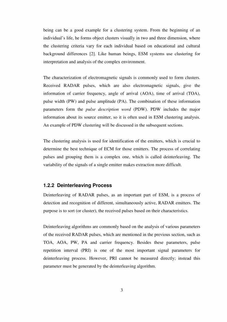
The first PRI cluster contains the main PRI value and the other one contains the ‘gap’
value. The relationship between mentioned PRI clusters and pointed PDW clusters is
shown in Figure 3.9. The dashed arrows show the relationship between PRI clusters
and PDW clusters and line arrows show the relationship within PRI clusters.
Figure 3.9 PRI and PDW Clusters of a Dwell PRI mode sequence
The PRI clusters’ PRI parameters and the pointed PDW values by their PDW Cluster
Pointers are set as output and a warning flag, sequence found, is sent to the operator.
After sending warning flag, the other PRI clusters are examined sequentially.

28
3.3.3 Staggered PRI Mode
If the proportion of the occurrences of first and second PRI clusters exceeds
stagger_occ threshold, this situation possibly points a stagger PRI mode RADAR.
However, how many different PRI clusters form this staggered series is unknown,
yet. To answer this question, Next Value parameter of second PRI cluster is
examined. If it points at the first PRI cluster, that means two different PRI cluster
form the stagger PRI series. The stagger chain is completed. Otherwise, the PRI
cluster that is pointed by Next Value parameter of second PRI cluster is examined.
The stagger detection process continues until one of the PRI cluster’s Next Value
parameter points to the first PRI cluster. All PRI clusters’ Occurrence parameters are
also examined and max_occ is updated during this process. At the end of the stagger
process, detected PRI clusters’ PRI parameters and the pointed PDW values by their
PDW Cluster Pointers are set as output, respectively and a warning flag, sequence
found, is sent to the operator. In Figure 3.10, an example of stagger PRI mode pulse
sequence is shown.
Figure 3.10 Stagger PRI Mode Pulse Sequence
The relationship between mentioned PRI clusters and pointed PDW clusters in a
level 3 stagger PRI mode sequence is shown the Figure 3.11. The dashed arrows
show the relationship between PRI clusters and PDW clusters and line arrows show
the relationship within PRI clusters.

29
Figure 3.11 PRI and PDW Clusters of a level 3 Stagger PRI mode sequence

30
Determination of the number of surrounding active RADARs and identification of
modes of each of them is continued until examining the last PRI cluster. All formed
PRI clusters are checked and interpreted by the Interpreter. Finally, the number and
modes of RADARs on the field are detected. At the end of the work, a final flag,
search_ends, is set in order to warn the operator. In Figure 3.12, the flowchart of the
Interpreter part is shown.

31
Figure 3.12 The Flowchart of Interpreter

32
CHAPTER 4
SURVEY ON DEINTERLEAVING ALGORITHMS
4.1 Folding Deinterleaving Algorithm
The folding deinterleaving algorithm is based on the principle that the pulse
sequence of a stable PRI mode RADAR is symmetric about any of its pulses.
Consider the pulse sequence received from 3 stable PRI mode RADARs, called A, B
and C, with different PRIs as shown in Figure 4.1. If this sequence is folded at time
tm that corresponds to a pulse of RADAR B, earlier and later pulses of B will occur at
the same instant, while pulses of A and C will not as shown, in Figure 4.2. Thus
pulses of RADAR B can be identified and taken out of the sequence. This procedure
is applied recursively on the remaining sequence in order to identify all stable PRI
mode RADARs. By defining a tolerance value to decide on overlapped pulses, the
algorithm can also handle jittered PRI RADARs. The overlapped pulses are assumed
to be emitted from the same emitter. The differences of TOAs of these pulses give
the PRI values of corresponding emitters.
Figure 4.1 3 interleaved stable PRI sequences

33
Figure 4.2 3 interleaved stable PRI sequences after folding
The experimental results point that the folding deinterleaving algorithm is limited up
to 1000 recorded pulses. This limitation increases the possibility to get the correct
result [6].
4.1.1 Criticism of the Algorithm
It can be easily noticed that there are lots of advantages of the folding deinterleaving
algorithm. It is easy to implement by using simple processors. It is fast and has
higher success rate in complex environments compared to other synchronized
deinterleaving methods. A pulse train containing 1000 pulses with 5 emitter sources
and 10 emitter sources is processed and success rate is 100% for environments that is
mentioned in Table 4-1 [6].

34
Table 4-1 Simulation Experimental Results of Folding Deinterleaving Algorithm
# of emitters Loss rate of
pulses Jitter rate
Probability of correct
computation of interleaving
frequency
0% 2% 100% 5
2% 5% 100%
0% 2% 100% 10
2% 5% 100%
However, there are also lots of disadvantages of this algorithm, if it is compared to
RCDA. First of all, checking all incoming pulse trains without their PDW parameters
(AOA, frequency, PW and PA), makes the pulse trains complex. This approach
decreases the success rate. If the following case is inspected, the vulnerability of
folding deinterleaving algorithm can be easily noticed. There are two emitters in the
field that has same PRI = T. Their pulses are transmitted in different frequencies. If
their pulses are received as one inside the other (interleaved), as shown in Figure 4.3,
the folding deinterleaving algorithm decide that there is a single emitter in the field
with PRI = T/2. This example demonstrates a serious vulnerability of the algorithm.
Figure 4.3 Two different emitter that has same PRI and different frequencies

35
The folding deinterleaving algorithm records TOA parameters of each pulse in a
sequence. This requires significant amount of memory for storage. It is a waste of
resources and also limits the number of pulses that can be processed at a time.
However, in RCDA, each pulse is processed as they arrive and only relevant
information is stored, reducing the amount memory for storage and removing the
limitation on the number of pulses that can be processed.
4.2 Difference Histogram Based Deinterleaving Algorithms
The original version of these algorithms is based on the so-called CDIF (cumulative
difference) [4] histogram of TOA differences of pulses. Modified and improved
version of this algorithm, based on the new sequential difference histogram
technique (SDIF) [8], is SDIF deinterleaving algorithm. Before the discussion of
CDIF and SDIF algorithms, the TOA difference histogram concept should be
described.
The TOA differences of the sequential pulses give an idea for PRI values of the
received pulse trains. Consider a list of TOAs. The first order TOA differences are
defined as the difference between any adjacent TOAs. The second order TOA
differences are defined as the difference between the TOAs of every other pulse.
Likewise, nth order TOA differences can be defined. In Figure 4.4, the orders of
TOA differences for a pulse train are shown.
Figure 4.4 The orders of TOA differences for a pulse train

36
In CDIF and SDIF algorithms, nth order TOA difference histogram is formed by the
nth order TOA differences of each reference pulse in the pulse train. The CDIF
algorithm is described in detail in the following section.
4.2.1 CDIF Algorithm
This algorithm is based on the CDIF histogram analysis [4]. By using TOA
differences, potential values of PRIs are calculated, which corresponds to histogram
peaks. As can be easily noticed from its name, Cumulative Difference, CDIF
algorithm forms histogram of TOA differences by using all orders of TOA
differences. In other words, cumulative TOA difference histograms are formed. An
nth order cumulative TOA difference histogram is the histogram of all TOA
differences of order less than or equal to n.
In CDIF algorithm, starting with c=1, the cth order CDIF histogram is formed and a
threshold is calculated. Each histogram value, and double that value, is compared to
the threshold, and if none of these couples exceeds the threshold, the next level (of
level c + 1) cumulative histogram is calculated [8].
After the identification of the potential PRI, the algorithm looks for a group of pulses
that form a periodical pulse train, with periods equal to PRI. Such a group of pulses
is set as a PRI sequence. If the search is successful, the PRI sequence is extracted
from the input buffer and the CDIF algorithm is applied on the remaining sequence.
This process is repeated as long as there are enough pulses in the input buffer. The
thresholds for histograms can be calculated by modeling the TOA of pulses as a
Poisson process. If more than one histogram value exceeds the threshold, the
sequence search is performed for every potential PRI value, starting from the lowest
[4].
4.2.2 SDIF Algorithm
The SDIF algorithm is a modification of CDIF algorithm. It consists of two parts,
namely the estimation of the PRI and the sequence search. The estimation of the PRI,

37
as the key part of the deinterleaving algorithm, is described below. The sequence
search part in the SDIF algorithm is the same as in CDIF algorithm.
Different from the CDIF histogram, in the SDIF histogram only single level of
differences exists, so the histogram is clearer than the corresponding CDIF
histogram. In CDIF algorithm, the cumulative histogram is compared to a threshold
and a value and twice that value is expected to pass the threshold to identify a PRI
sequence. Then, that PRI sequence is searched for in the input list. SDIF algorithm
looks for a single threshold crossing since a PRI sequence search is eventually
necessary. PRI sequence search for a given PRI is an easier process than the
computation of the next level histogram and thus SDIF algorithm is less
computationally extensive.
When the first difference is computed, if only one histogram value exceeds the
threshold, that value becomes the potential PRI for which a sequence search will be
performed. However, if many emitters are present, the first difference histogram
produces a few values exceeding the threshold, none of which corresponds to the
right PRI value. That is why the next difference has to be calculated without a
sequence search. The reason of skipping the first difference in the case of three
interleaved radar signals can be seen from Figure 4.5. In this scenario, two classic
RADARs (with PRIs of 217 and 248) and one stagger RADAR (with a stagger frame
rate of 318) are present. The first difference in the SDIF histogram does not present
the true PRI values, because they are hidden in higher differences.

38
Figure 4.5 SDIF histogram of the TOA first difference in a complex radar environment [8]
If the random jitter of PRI values is analyzed, similar PRI values in the SDIF
histogram, grouped around the true PRI value, can produce histogram values
exceeding the threshold. If the range of PRI values is no greater than the permitted
tolerances, the sequence search is performed for the central value, which represents
the potential jittered PRI. Figure 4.6 illustrates this case: the histogram values
exceeding the threshold correspond to one detected emitter with a random jitter PRI
of central value 263.

39
Figure 4.6 SDIF histogram of random jittered PRI signal [8]
If in the case concerned great amounts of pulses are missing, the harmonics of the
basic PRI can produce significant components in the SDIF histogram. These values
could be so dominant as to exceed the threshold. This is not a problem if the
histogram value corresponding to the true PRI value also exceeds the threshold, since
the PRI analysis and the sequence search start from the lowest PRI having a
histogram value that exceeds the threshold [8]. However, this situation could be a
great disadvantage to detect correct PRI sequence, if the true PRI sequence does not
exceed the threshold. In this case, the harmonics are sensed as true PRI and false PRI
value occurs in the output. Figure 4.7 shows the SDIF histogram with a true PRI
value of 428. However only its first harmonic of 856 exceeds the threshold and
appears as a true PRI value.

40
Figure 4.7 SDIF histogram of TOA for many missing pulses[8]
In order to avoid false detections, subharmonic checking is done, that is the
histogram maximum is found. If it does not exceed the threshold, the first (lowest)
value exceeding the threshold is checked. If the corresponding PRI value presents
some harmonic of the PRI value corresponding to the histogram maximum, the
maximum then becomes the potential PRI for which the sequence search is
performed. If the lowest PRI value which exceeds the threshold is not a multiple of
the histogram maximum PRI value, the sequence search is performed for all PRI
values which exceed the threshold, starting with the lowest [8]. This analysis of
harmonics and subharmonics represent a modification of the CDIF algorithm [4].
This checking could be misleading in complex environments. Also it could take
significantly much time for detecting the true PRI; since the harmonics could also be
true PRI values.
As it can be easily understood, threshold choice is very important in SDIF histogram
for reliable detection of true PRI values. The threshold value follows the distribution
function of the process to prevent the detection of false alarms. As leading edge of
pulses could be observed as random Poisson points, there can be various types of

41
threshold value calculations. The simulation results for different threshold values can
be seen in Table 4-2, where τ is the bin number in the SDIF histogram.
Table 4-2 Simulation Experimental Results of SDIF Algorithm using only PRI
Threshold function
Number of successfully detected
RADARs
Number of false RADARs
Processor time (flops)
# of RADARs
5 7 3 5 7 3 5 7 3
)exp( τ−
5 7 3 0 1 0 285K 341K 188K
τ/1 2 3 2 5 10 2 823K 1.32M 514K
τ/1 4 5 3 2 5 1 489K 827K 333K
The effects of changing threshold function can be noticed better in Figure 4.8.
Figure 4.8 Different forms of threshold in SDIF histogram [8]

42
The processor time results of SDIF histogram deinterleaving algorithm in Table 4-2,
may not be compared to the timing results of RCDA, because parameters of
RADARs, i.e. frequency, PW and PA, are not considered yet in SDIF histogram
deinterleaving algorithm. In the following section, SDIF algorithm with multiple
parameter is explained and the comparisons between two algorithms can be
discussed after the following explanation.
4.2.2.1 Multiple Parameter Deinterleaving With SDIF
The algorithm is based on multiple parameter deinterleaving. The incoming pulses
are sorted by azimuth (DOA), frequency, PW and TOA. By DOA and frequency
filtering, incoming pulses are split and forms clusters. TOA difference histograms are
processed sequentially. Stable and agile RADARs cause the main challenge in this
algorithm. The goal is correct grouping of RADARs despite their overlapping
characteristics. This is not a new algorithm, but comparison of speed and reliability
become main target [8]. Similar to RCDA, clustering process is the first part of the
algorithm, but differently, parameters have priorities in the clustering process.
Choosing histogram group boundaries is important and affects the performance of
the algorithm. Local minima of the average histogram values are declared as group
boundaries. This is declared as one possible solution [8]. The clustering is done on
azimuth parameter and then the next parameter, frequency is used for better
clustering.
Frequency parameter is important for frequency agile RADARs. These kinds of
RADARs cause false clustering problem. In the azimuth cluster groups, sub
frequency clusters are formed. However this kind of clustering could break the
correlation of azimuth and frequency and detecting RADARs correctly becomes
almost impossible. So, a new priority of parameters is assigned. PRI value is used as
the second clustering parameter and frequency has the third priority.
Frequency histogram shows one significant peak for RADARs with fixed carrier
frequencies. If multiple peaks are observed in the frequency histogram, a frequency

43
agile RADAR is present, so the frequency histograms are only used to identify the
type of the detected RADAR, and not significant for clustering.
The clusters that have same azimuth, PRI and frequency, are assumed to be stagger
RADAR signals. Stagger analysis is done last. The simulation results are shown in
the following table [8].
Table 4-3 Simulation Experimental Results of SDIF Algorithm using multiple parameters
Number of RADARs in the
environment
Successfully Detected RADARs
False RADARs Processor time
(flops)
2 2 0 56271
4 4 1 326212
5 5 0 282097
10 9 3 623417
4.2.3 Criticism of the Algorithm
The results of the SDIF deinterleaving algorithm seem satisfactory, if the success
ratios are examined. Most of the RADARs are detected correctly. The tools that are
used for implementation are old fashioned, which can be an excuse for slow handling
of process. However, number of processor flops gives a chance to compare SDIF
deinterleaving algorithm and RCDA. If the numbers of cycles are compared, it will
be seen that RCDA is much faster. Besides the cycling time, using hardware tools
(FPGA) makes RCDA more efficient and faster. The results of RCDA are given in
the following chapter.
SDIF deinterleaving algorithm forms histograms after collecting incoming pulse
parameters. It waits the end of streaming data for starting the main process. The
major advantage of RCDA over SDIF deinterleaving algorithm is starting to form its
clusters during the data flow. It updates the clusters in each incoming pulse. If two

44
mentioned algorithms are started at the same time, such a situation occurs: when
SDIF deinterleaving algorithm is at the beginning of forming histogram and
clustering, RCDA just finishes the same work, which makes it much more preferable.
In the SDIF histogram part, determining optimal detection threshold value takes lots
of processor flops, which also decreases the speed of the process. In RCDA, the
threshold value is constant and user defined which is mentioned in the previous
chapter. This can be considered as a disadvantage for RCDA, but some trade-offs
should be done in hardware implementation. First of all, taking threshold as a
constant, but not a Poisson distribution function [7], eliminates a large amount of
process time. Also using complex mathematical functions, like dividing, power,
exponential, root and etc., is not preferable in hardware implementations, because
such operations occupy significant logic units and block memories. Despite the speed
and area disadvantages, determining the threshold by using Poisson distribution
could have some advantages for true PRI detection in complex environments.
Clustering process in SDIF deinterleaving algorithm has some important differences
as compared to RCDA. It uses parameters of pulses in a priority order while splitting
the cluster groups. Azimuth parameter is chosen as first priority parameter [8], but
this choice could bring some disadvantages for detecting correct PRI sequences.
Reflection and deflection of main signal corrupt the measurement of azimuth (or
AOA), which makes this PDW parameter unreliable. This issue is discussed in detail
in Chapter 2.
As it can be easily noticed from the situation of parameter measurement problems, it
may be necessary to adjust the priority of the pulse parameters from case to case, so
the algorithm may not be stable for each scenario. It should be adjusted to the
environment, which is not desirable for user. There are no such situations in RCDA,
as priority is not handled while forming PDW clusters.
Discarding the parameter, PW, in SDIF deinterleaving algorithm is another
discussable approach. This parameter could help separating the clusters of PDW. It
seems that the number of clustering parameters in SDIF deinterleaving algorithm is

45
kept small because of the sub clustering approach. More parameters make the
algorithm more complex and hard to implement.
Another comparison can be done between SDIF deinterleaving algorithm and
RCDA, among the histograms of PRI values. In SDIF deinterleaving algorithm,
avoiding harmonics and subharmonics of a true PRI value is a problem. Complex
threshold calculations and analysis are done in order to suppress those harmonics.
However, Next Value and Previous Value parameters of PRI clusters in RCDA
prevent harmonics and subharmonics of a true PRI value. Harmonics can be only
seen if missing pulses or false alarms occur. In such a situation, occurrence threshold
value is used to suppress them in order to avoid processing harmonic PRI values as
true PRIs.
SDIF deinterleaving algorithm has great advantages over previous deinterleaving
algorithms [8]. It uses clustering, optimal detection of threshold and analysis of
histogram. However, speed, implementation issue and some algorithm choices,
which are discussed above, bring major disadvantages to this algorithm as compared
to RCDA.

46
CHAPTER 5
SOFTWARE IMPLEMENTATION OF ANALYZER
The software implementation of Analyzer is done by using MATLAB 7.4.0 (R2007a)
tool in order to test the reliability of the RCDA. The software implementation
provides input flexibility and more insight on the operation of the algorithm. Using
this software, the algorithm can be tested for various user defined parameters and
different environment variables such as the number of RADARs and their types,
noise and jitter values. The steps of the RCDA implementation and analysis of the
simulation results are given in the following sections.
5.1 Implementation of the MultiRadar Simulator
The MultiRadar simulator is implemented in order to generate the PDW parameters
of various numbers of different RADARs. The pulse sequence, which includes PDW
parameters of various RADARs, is simulated. The output of the MultiRadar
simulator is a sequence of interleaved pulses that are emitted from different
RADARs, and used as input to the implemented version of RCDA. Number of
generated RADARs and their modes, PDW parameters and PRI values are
determined by the user.
The percentage of variance of frequency is also specified by the user in order to
generate frequency agile or frequency hopping RADARs. The percentages of
variances of PW, PA and PRI jitter value are also input to generate RADAR pulses
that are received in noisy environments. The ratio of missing pulse or false alarm to
total number of generated pulse is also an input of MultiRadar simulator. It is used to
generate missing pulse or false alarm situations.

47
The PDW parameters of each pulse are generated by adding jitter and noise values.
The percentage of jitter and noise input values are the max values. The max values
are multiplied by a random value before adding to the PDW parameters. The random
values are generated by Uniform distribution function. Each RADAR’s pulse train
starts with a random offset value. As a result, MultiRadar simulator generates
different pulse trains with same input values for each trial. The block diagram of
MultiRadar simulator is shown in Figure 5.1.
Figure 5.1 Block Diagram of MultiRadar Simulator

48
5.2 Implementation of the Analyzer
The implementation of Analyzer is done by using MATLAB 7.4.0 (R2007a) tool by
following the steps of RCDA that is described in detail in Chapter 3. The pulse train
that includes PDW parameters of each generated pulse by MultiRadar simulator is
one of the inputs of the Analyzer. The other inputs are delta values for each PDW
parameters, threshold values for Occurrence parameter of PRI clusters and
search_limit, which are described in detail in Chapter 3.
5.2.1 Simulation Results of Analyzer
The simulations are done for different scenarios. The variables of each scenario are
the number of RADARs, percentage of jitter and noise values and percentage of
missing pulses or false alarms. The simulations are done for simple to complex
environments.
5.2.1.1 Different Environments for Simulating Real Scenarios
Different environments are generated by using MultiRadar simulator. Simulations of
the Analyzer are done for each environment. In each case, 100 trials are done and
success rate of each trial is given. The success rate is calculated in each trial as
shown in Eq. (5-1).
100_
___ ×=
radarsgenerated
radarsfoundcorrectlyratesuccess (5-1)
In the following success analysis, the variables of the environment are changed in
each case. Number of RADAR takes values of 1, 3, 5 and 8; jitter and noise
percentages take values of 0%, 2% and 5% and missing pulse percentage takes
values of 2%, 5% and %10, respectively. Different RADAR modes are chosen in
multi RADAR scenarios. The results are shown in Table 5-1 and Table 5-2.

49
Table 5-1 Simulation Results of RCDA for environment of 1 and 3 RADARs
# of
RADARs
Jitter and
Noise rate
Missing
pulse rate Success Rate
2% 100%
5% 100% 0%
10% 100%
2% 100%
5% 100% 2%
10% 100%
2% 100%
5% 100%
1
5%
10% 100%
2% 100%
5% 100% 0%
10% 100%
2% 100%
5% 100% 2%
10% 100%
2% 100%
5% 100%
3
5%
10% 100%

50
Table 5-2 Simulation Results of RCDA for environment of 5 and 8 RADARs
# of
RADARs
Jitter and
Noise rate
Missing
pulse rate Success Rate
2% 100%
5% 100% 0%
10% 100%
2% 100%
5% 100% 2%
10% 100%
2% 100%
5% 100%
5
5%
10% 100%
2% 100%
5% 100% 0%
10% 100%
2% 100%
5% 100% 2%
10% 100%
2% 98%
5% 98.88%
8
5%
10% 98.88%

51
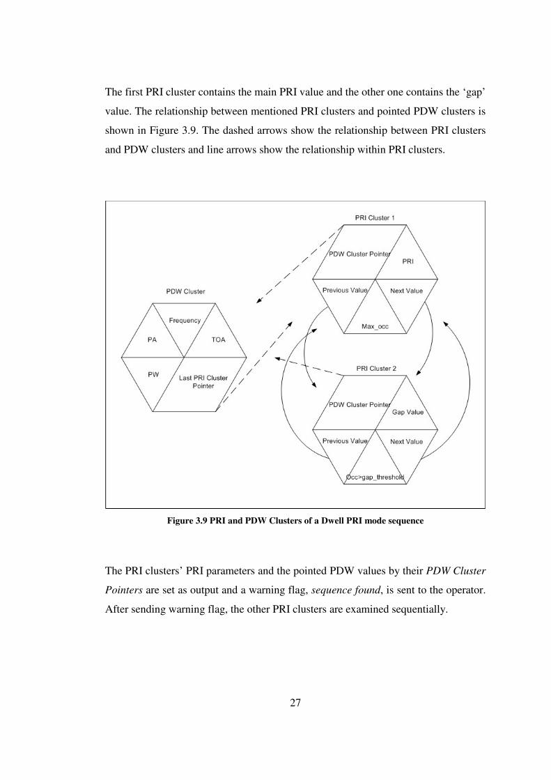
An inspection of the above success analysis shows that, RCDA is a satisfactory
algorithm for different cases that simulate real environment situations. Only, in the
case that includes 8 RADARs and 5% of jitter and noise rate, the success rate does
not reach value of 100%.
Although the above success analyses are satisfactory, the limitations of RCDA are
still unknown. In order to investigate the limits for different environment parameters,
the following success analyses are done.
5.2.1.2 Limits of RCDA for Different Environment Parameters
As mentioned previously, there are three environment parameters in each case:
number of RADARs, jitter and noise rate, missing pulse or false alarm rate. In the
following simulations, only one of these parameters is changed and success analysis
is done. In each analysis, Monte Carlo simulation is used. 100 trials are done for each
value of the variable parameter and success rate is calculated. New RADARs are
generated by MultiRadar simulator in each trial.
The simulation results for jitter and noise rate variable is shown in Figure 5.2. In this
case, missing pulse or false alarm rate is 0% and number of RADAR is ‘1’. The
mode of RADAR is chosen as equal probability of stable, dwell and stagger PRI
modes.
Up to 16% jitter and noise, the algorithm has a success rate of 100%. For a typical
environment, this result does not seem unsatisfactory. The noise rate is reversely
proportional to SNR, which is related to the receiver of the system. Increasing SNR
decreases the noise rate, which is better for correct detection of RADARs. SNR value
cannot be adjusted or changed by RCDA. If the jitter rate is considered, the delta
values of PRI and frequency should be increased by the increasing of jitter rate in
order to reach better success rates. In this scenario, the delta values are kept constant.
52
Figure 5.2 Success Analysis for variable values of jitter and noise rate
The simulation results for missing pulse or false alarm rate variable is shown in
Figure 5.3. In this case, jitter and noise rate is 0% and number of RADAR is ‘1’. The
mode of RADAR is chosen as equal probability of stable, dwell and stagger PRI
modes.
Up to 12% missing pulse or false alarm rate, the algorithm has a success rate of
100%. The missing pulse rate is also related to SNR value and SNR value is related
to receiver of the system as mentioned before. For 100% success rate 88% of the
pulses should be received correctly.

53
Figure 5.3 Success Analysis for variable values of missing pulse or false alarm rate
Simulations for number of RADARs variable are done and success rate is 100% up
to 59 RADARs which is the largest number of RADARs that can be simulated using
the implemented software due to memory and processing power limitations. The
modes of RADARs are chosen randomly. In this case, both jitter and noise rate and
missing pulse or false alarm rate are 0%. The consequence of this analysis is that the
success rate is independent from number of RADARs when the other parameters
have the value of 0% due to the clustering structure of the RCDA. As there is no
jitter, noise, missing pulse or false alarms, the PDW and PRI clusters includes true
parameters, so there is no false detection of RADARs. Therefore, the success
analysis is done for some different values of jitter and noise rate and missing pulse or
false alarm rate. The simulation results are shown in Figure 5.4, Figure 5.5, Figure
5.6 and Figure 5.7.

54
Figure 5.4 Success Analysis for different numbers of RADARs for 2% jitter and noise rate
and 5% missing pulse or false alarm rate
Figure 5.5 Success Analysis for different numbers of RADARs for 2% jitter and noise rate
and 10% missing pulse or false alarm rate

55
Figure 5.6 Success Analysis for different numbers of RADARs for 5% jitter and noise rate
and 2% missing pulse or false alarm rate
Figure 5.7 Success Analysis for different numbers of RADARs for 5% jitter and noise rate
and 10% missing pulse or false alarm rate

56
5.3 Evaluation of Simulation Results
The simulations of RCDA are done for different environment parameters and the
results are shown in the previous section. The results seem satisfactory for real
environment simulations. Some recommendations are described below for better
results of RCDA.
First of all, delta values should be set properly before the beginning of the process.
Otherwise the PDW clusters cannot be formed correctly, especially in the case of
high jitter and noise rates. In that case, PDW parameters of pulses, which are emitted
from same RADAR, can fall into different PDW clusters because of the high
difference level of the PDW parameters. So the probable RADARs cannot be
detected correctly, which is not desired.
For correct detection of RADARs, PDW parameters should be measured correctly. It
is curial for PDW clustering. If more than one RADARs’ pulses’ PDW parameters
are measured as the same PDW parameters, they cannot be detected as different
RADARs. In such cases, correct detection of RADARs cannot be done.
If there are at least two RADARs that emit pulses, which have same PDW
parameters, they cannot be detected by using RCDA. For such cases, AOA parameter
should be added to the PDW clusters of the RCDA. Because PRI clusters, which
have same parameters of PDW Cluster Pointer, are interpreted as belonging to same
PRI sequence and hence same RADAR. In order to deinterleave pulse trains of
RADARs, the pulse trains of each RADAR should have different PDW parameters.
In fact, at least one PDW parameter must different for pulses of different RADARs
in a real environment. As an example, consider a scenario in which there are more
than a RADAR that emit pulses with same carrier frequency and PW. Their distances
to the receiver are equal, so PA parameters of pulses from these different emitters are
also the same. However, the AOA parameter must be different since these RADARs
are assumed to be different. In such a scenario, the pulse trains can be deinterleaved
using AOA parameter in the PDW. This scenario is depicted in Figure 5.8.

57
Figure 5.8 Same RADARs with same distances to receiver
Another interesting scenario might include more than a RADAR that emit pulses
with same carrier frequency, PW and AOA. The distances of these RADARs to the
receiver must be different since otherwise we would have identical RADARs
operating at the same geographical location which is not a realistic case. Thus the PA
parameters of these RADARs cannot be same and pulses of pulse train that belong
to different RADARs do not fall into same PDW cluster in RCDA. This scenario is
depicted in Figure 5.9.

58
Figure 5.9 Same RADARs with different distances and same angle to receiver
As a result, if an ideal receiver receives the pulses that are emitted from the
RADARs in the environment, the measured PDW parameters of each pulse train that
is emitted from one RADAR are different from the PDW parameters of pulses that
are emitted from another RADAR. So, RCDA can deinterleave pulse trains and is
used to detect RADARs in the environment correctly.
Consequently, RCDA gives satisfactory results, if the conditions that are explained
above are satisfied and values of inputs are set properly for each environment.
However, operation on real data is not done during the software implementation
simulations. Antenna rotation and pattern effects on PA are not considered in these
simulations. As mentioned before, it is assumed that the PDW parameters are
produced perfectly as input to the RCDA by a previous system.
59
CHAPTER 6
HARDWARE IMPLEMENTATION OF ANALYZER
In this chapter, the hardware implementation of the Analyzer and the hardware
simulation results are discussed. The reliability of RCDA is discussed in the previous
chapter and the timing analysis is emphasized in this chapter. The simulation results
are discussed in detail.
6.1 Hardware Implementation
The implementation of the Analyzer is done in VHSIC Hardware Description
Language (VHDL) by using Project Navigator 6.3 program tool of Xilinx Inc. First
of all, the project is generated and properties of it are set by following the steps of
project navigator. In Figure 6.1, the selected properties of project are shown. The
XC2VP50 of Virtex II Pro device family is chosen. It is a mature FPGA type of that
family and a preferable one for high speed implementations.

60
Figure 6.1 Project Properties of Analyzer
The structure of the project is decided as follows: the entity, the Analyzer, is the top
level part of project and components of it, the Arranger and the Interpreter, are sub
level parts. This is also visualized in Figure 3.1. The structures are based on state
machines and Intellectual Property (IP) cores. IP cores that are used in the Arranger
and the Interpreter are adders and Block RAMs (BRAMs) of FPGA. Proper values
are set for all IP cores before they are generated.
After building the design in VHDL, the project is synthesized. The device utilization
summary of the Analyzer is shown in Figure 6.2.
Figure 6.2 Device utilization summary of the Analyzer

61
6.2 Simulation Results of Hardware Implementation
The simulations are done by using Modelsim SE 5.7e tool of Modeltech in order to
test the timing performance of the Analyzer. In the simulation, the clock period is set
to 10 ns. The timing of two process are crucial in the hardware implementation
simulations, these are time duration of updating clusters in each arrival of pulse that
is done by the Arranger and time duration of interpretation that is done by the
Interpreter.
For timing analysis simulations, an environment with two different RADARs is
chosen. One of the RADARs is in stable PRI mode and the other one is in level 4
stagger PRI mode. The carrier frequency, PW and PA of the pulse trains of these
RADARs are different. The pulse trains that are emitted from RADARs are
interleaved. The time duration of updating clusters is shown in Figure 6.3.
Figure 6.3 Time duration of updating clusters
The time duration between the arrival of a new PDW and the end of updating PDW
clusters and PRI clusters is 300 ns, i.e., 30 clock times. This duration can increase in
more complex environments. In this time duration, the Arranger is busy and if a new
PDW arrives, it is pipelined. However, this pipelining has a limit, i.e., if two inputs
arrive to the system with an interval less than 100 ns, the Arranger cannot process
both of them. It misses one of those inputs and this is not desirable.

62
Another time analysis is done to measure the time duration between triggering of the
Interpreter and the end of interpretation of probable RADARs, which is called the
time duration of interpretation. The time duration of interpretation is shown in Figure
6.4.
Figure 6.4 Time duration of interpretation
The time duration between rising of arranged signal, which is the trigger for the
Interpreter, and rising of sequence_found signal is 150 ns, i.e., 15 clock times. This
time duration is also the time duration of interpretation and can increase in more
complex environments, because it is directly proportional to the number of PRI
clusters that are formed by the Arranger.
6.3 Criticism of Simulation Results
The simulations of hardware implementation of the Analyzer are done in order to
determine the limits of crucial timing process and the results are shown in the
previous section. The timing results seem satisfactory. If the timing results of
previous deinterleaving algorithms, which are discussed in detail in Chapter 4, and

63
the Analyzer are compared, it can be easily seen that the Analyzer processes much
faster than the others. Implementation by using FPGA provides major advantage to
the Analyzer, because real time clustering cannot be done without FPGA. The other
algorithms collect the data of pulses first and start to deinterleave the pulse trains.
However, the Analyzer makes real time clustering in each arrival of data of pulse. It
does not only collect but also clusters the PDWs and probable PRIs.
When the Analyzer finishes clustering process and starts the interpretation, the other
systems, which are described in detail in Chapter 4, just start their deinterleaving
processes, which take time duration of at least a few microseconds. However, the
Analyzer finishes the interpretation in less than a microsecond. The pulse processing
rate of Analyzer is also faster. In average, more than 8 million pulses can be
processed in a second.
In order to improve the hardware implementation, improved versions of FPGAs can
be used. Virtex 5 family FPGAs that are the products of Xilinx Inc. can be used for
faster clock times. Using faster clocks provides less time duration of updating
clusters, making it possible to process more closely spaced pulses and decreasing the
probability of missing a pulse. Faster clock also decreases the time duration for
interpretation and improves the performance of the Analyzer. Using improved FPGA
versions also decreases the area that is occupied by the implemented Analyzer,
because the slice structure of new FPGAs is designed more efficient than the
previous ones.

64
CHAPTER 7
CONCLUSIONS
In this thesis, a new deinterleaving algorithm that is called RCDA, which can be used
as a part of an ESM system, and its implementation by using an FPGA, is studied.
The function of implemented RCDA is interpreting the complex electromagnetic
military field in order to detect and determine different RADARs and their types by
using incoming RADAR pulses and their PDWs. Real time processing of PDW is the
most important motivation behind this work. It is assumed that RADAR signals in
the space are received clearly and PDW of each pulse is generated as an input to the
implemented RCDA system.
PDW and PRI clustering and a new interpreting process are used in RCDA in order
to deinterleave the RADAR pulses. Reliability of the algorithm is tested by using
software implementation of it. For hardware implementation, FPGA is used to
achieve a more efficient and faster system. The simulation results of software and
hardware implementations are shown and discussed. After the simulation results, the
comparison of implemented RCDA system and the previous systems, which are
discussed in detail in Chapter 4, is done. The comparison results are determined in
the following.
First of all, most of the deinterleaving algorithms in the literature collect RADAR
pulse’s data and wait to start the deinterleaving process until the end of this
collection process. This approach may include some disadvantages for fast
processing. However, the process starts in RCDA by the arrival of the first pulse,
because real time processing is done in RCDA. PDW and PRI clusters are updated in
each pulse’s arrival. When the other systems stop collecting data of pulses and start
deinterleaving of pulse trains; the Analyzer, which is the implemented version of
RCDA, finishes forming PDW and PRI clusters and starts interpreting of probable

65
RADARs on the field. This is one of the significant advantages of the Analyzer over
the other deinterleaving algorithms that are examined in detail in Chapter 4.
Another advantage of the Analyzer is the more efficient use of memory. As the other
deinterleaving algorithm systems collect and record each RADAR pulse’s data, they
need a significant amount of memory, which the Analyzer does not require, because
it does not record each pulse’s data separately. The Analyzer just updates PDW and
PRI clusters by the arrival of each pulse’s data. This conservation of memory is also
very important in hardware implementations.
Determining threshold value for PRI histograms is another difference between
RCDA and the previous Deinterleaving algorithms. In the CDIF [4] and SDIF [8]
deinterleaving algorithms’ histogram parts, determining optimal detection threshold
value takes lots of processor flops, which also decreases the speed of the process, and
requires large amount of memory. In RCDA, the threshold value is constant and user
defined. This can be seen as a disadvantage for the Analyzer, but some trade-offs are
done in hardware implementation. First of all, taking threshold as a constant, but not
a Poisson distribution function [7], decreases the process time. Using complex
mathematical functions, like dividing, power, exponential, root and etc., is not
preferable in hardware implementations, because such operations occupy significant
logic units and block memories in FPGA. Despite the speed and area disadvantages,
determining the threshold by using Poisson distribution could provide more precise
results for true PRI detection in more complex environments.
In RCDA, there is no priority for PDW parameters during PDW clustering process.
However, in multiple parameter deinterleaving algorithm [8], the priorities are given
to each PDW parameter and forms sub clusters, i.e., AOA has the first priority and
top level clusters are formed respecting this PDW parameter. This approach may be
unsafe, because if measurement of AOA is not done properly, as discussed in
Chapter 2 in detail, all cluster chains may collapse. In this situation, deinterleaving of
RADAR pulse trains becomes impossible. So giving no priority to PDW parameters
during PDW clustering is the approach chosen in RCDA.

66
Harmonics analysis of true PRI values is another important process in deinterleaving
algorithms. In CDIF [4] and SDIF [8] deinterleaving algorithms, this analysis is done
to determine the true PRI values. This process takes a lot of flops of time and is not
preferred in RCDA, because RCDA is designed in order to be used in hardware
implementation. The chains between PRI clusters are provided by the parameters,
Next Value and Previous Value, of PRI clusters in RCDA. They prevent false
detection of probable PRI values and discard the harmonic analysis from the
algorithm.
Discarding AOA from the PDW parameters that are used for PDW clustering is a
discussable approach in RCDA. For land or navy platform RADARs, reflection and
deflection of the main signal cause wrong measurement of AOA that is also
mentioned in Chapter 2 in detail. This is the main reason for discarding AOA.
However, AOA can be easily added as another PDW clustering parameter to RCDA,
if it is needed. This modification of RCDA can be done for more complex
environments that exclude reflection and deflection.
Although the Analyzer has lots of advantages and performs well that can be easily
noticed form the simulation results, it has some disadvantages. One of the
disadvantages is the following: if the missing pulse or false alarm situations occur in
the last PRI period of a dwell or stagger PRI mode pulse sequence, the chain between
PRI clusters that are provided by Next Value and Previous Value parameters of PRI
clusters is broken, because the missing pulse or false alarm situations causes to set
wrong value to these parameters.
The other vulnerability of RCDA is that if there are more than one RADARs that
have pulse trains with the same PDW parameters, these RADARs cannot be
distinguished and probably detected as single RADAR.
In the hardware implementation, the VirtexII Pro family of FPGAs are used. Using
FPGA provides the major advantage to the Analyzer. If the comparison of speed
performance is done between the Analyzer and the other deinterleaving algorithm
systems that are also discussed in Chapter 4, it is easily noticed that the Analyzer is

67
much faster than the others because of the hardware implementation of it. However,
the speed and occupation of area results can be improved by using new products of
FPGAs, i.e., Virtex 5 family FPGAs that are produced by the Xilinx Inc. The slice
structure is improved in these products. This improvement provides less occupation
of area. Also the clock period can be decreased significantly in order to achieve
faster performance.
The implementation of the algorithm should be tested with real data as a future work.
In this work, all tests and simulations are done with produced inputs as mentioned
before. In the tests with real data, digital receivers can be used for better results,
because digital receivers give more precise outputs to the Analyzer than the analog
receivers.
As mentioned before, real time processing is the main motivation behind this work,
so all approaches, choices and trade-offs are decided to implement an efficient
deinterleaving algorithm for an FPGA implementation, which processes with a high
speed and occupies less area. The simulation results of performance, reliability and
speed seem satisfactory.

68
REFERENCES
[1] Skolnik, M. I., “Radar Handbook”, Second Edition, McGraw Hill 1990.
[2] Güvenlik, A.R., “Clustering Techniques for Emitter Identification In
Electromagnetic Warfare”, Ms. Thesis, Middle East Technical University,
December, 1999.
[3] Güven, E., “Emitter Identification in Electronic Warfare by the Use of Clustering
Techniques”, Ms. Thesis, Middle East Technical University, September, 1994.
[4] Mardia, H.K., “New techniques for the deinterleaving of repetitive sequences”,
IEE Proc. F, Commun. Radar & Signal Process, 1989.
[5] Chan, Y.T., Chan, F., Hassan, H.E., “Performance Evalution of ESM
Deinterleaver Using TOA Analysis”, Department of Electrical and Computer
Engineering, Royal Military Collage, Kingston, Canada, 1993.
[6] Quan, G.R., Sun, Y.S., Chen, B., “Folding Deinterleaving Algorithm For
Multiple Mixed Pulse Trains With Pulse Repetition Intervals”, School of Software,
Harbin Institute of Technology in Weihai, 2006.
[7] Papoulis, Athanasios, “Probability, Random Variables and Stochastic
Processes”, McGraw-Hill Inc. 1991.
[8] Milojevic, D.J., Popovic, B.M., “Improved Algorithm for the Deinterleaving of
Radar Pulses”, IEE Proceedings-F, Vol. 139, No. 1, 1992.

69
[9] “Virtex-II Pro Platform FPGA Handbook”,Xilinx Inc, 2002.
[10] “Xilinx System Generator for DSP v6.3 User Guide, A Tutorial Indroduction”,
Xilinx Inc, 2004.
[11] Hwang, J., Milne, B., “System Level Tools for DSP in FPGAs”, 2001.
[12] Mazor, S., Langstraat, P. “A Guide To VHDL, Second Edition, Synopsys Inc.,
1993.

70
APPENDIX A
A.1 FPGA’s
A field programmable gate array (FPGA) is a general-purpose integrated circuit. It is
"programmed" by the designer rather than the device manufacturer. Unlike an
application-specific integrated circuit (ASIC), which can perform a similar function
in an electronic system, an FPGA can be reprogrammed, even after it has been
deployed into a system.
An FPGA provides the user with a two-dimensional array of configurable resources
that are used to implement a wide range of arithmetic and logic functions. These
resources include dedicated 18x18 bit multipliers, dual port memories, lookup tables
(LUTs), registers, tristate buffers, multiplexers, and digital clock managers.
FPGAs are high performance data processing devices. FPGA performance is derived
from the ability they provide to construct highly parallel architectures for processing
data. Compared to a microprocessor or DSP processor, where performance is tied to
the clock rate at which the processor can run, FPGA performance is tied to the
amount of parallelism that can be brought to bear in the algorithms making up a
signal processing system. Currently system frequencies of 100-200 MHz are
commonly used today. A combination of increasingly high system clock rates and
highly distributed memory architecture gives the system designer an ability to exploit
parallelism in DSP applications that operate on data streams. For example, the raw
memory bandwidth of a large FPGA running at a clock rate of 150 MHz can be
hundreds of terabytes per second. [10]
There are wide ranges of DSP applications as digital up/down converters, digital FIR
filters etc that can be implemented only in custom integrated circuits (ICs) or
specifically in an FPGA. Advantages of using an FPGA include significantly lower

71
non-recurring engineering costs than those associated with a custom IC (FPGAs are
commercial off-the-shelf devices), shorter time to market, and the configurability of
an FPGA, which allows a design to be modified, even after deployment in an end
application.
Figure A.0.1 Virtex Family FPGA Logic Slice
Logic Slice is the fundamental unit of the logic fabric array. It is instructive to take a
closer look at the Virtex family logic slice construction, which is given in Figure
A.0.1. Each logic slice contains two 4-input lookup tables (LUTs), two configurable
D-flip flops, multiplexers, dedicated carry logic, and gates used for creating slice
based multipliers. Each LUT can implement an arbitrary 4-input Boolean function.
Coupled with dedicated logic for implementing fast carry circuits, the LUTs can also
be used to build fast adder/subtractors and multipliers of essentially any word size. In
addition to implementing Boolean functions, each LUT can also be configured as a
16x1 bit RAM or as a shift register (SRL16). An SRL16 shift register is a
synchronously clocked 16x1 bit delay line with a dynamically addressable tap point.

72
In recent years, field-programmable gate arrays (FPGAs) have become key
components in implementing high performance digital signal processing (DSP)
systems, especially in the areas of digital communications, networking, video, and
imaging. The logic fabric of today's FPGAs consists not only of look-up tables,
registers, multiplexers, distributed and block memory, but also dedicated circuitry for
fast adders, multipliers, and I/O processing (e.g., giga-bit I/O). The memory
bandwidth of a modern FPGA far exceeds that of a microprocessor or DSP processor
running at clock rates two to ten times that of the FPGA. Coupled with a capability
for implementing highly parallel arithmetic architectures, this makes the FPGA
ideally suited for creating high-performance custom data path processors for tasks
such as digital filtering, fast Fourier transforms, and error correcting codes [11].
73
APPENDIX B
B.1 Information About VHDL
VHDL is the VHSIC Hardware Description Language. VHSIC is an abbreviation for
Very High Speed Integrated Circuit. It can describe the behavior and structure of
electronic systems, but is particularly suited as a language to describe the structure
and behavior of digital electronic hardware designs, such as ASICs and FPGAs as
well as conventional digital circuits.
VHDL is a notation, and is precisely and completely defined by the Language
Reference Manual (LRM). This sets VHDL apart from other hardware description
languages, which are to some extent defined in an ad hoc way by the behavior of
tools that use them. VHDL is an international standard, regulated by the IEEE. The
definition of the language is non-proprietary.
VHDL is not an information model, a database schema, a simulator, a toolset or a
methodology, but, a methodology and a toolset are essential for the effective use of
VHDL.
Simulation and synthesis are the two main kinds of tools which operate on the
VHDL language. The Language Reference Manual does not define a simulator, but
unambiguously defines what each simulator must do with each part of the language.
VHDL does not constrain the user to one style of description. VHDL allows designs
to be described using any methodology - top down, bottom up or middle out. VHDL
can be used to describe hardware at the gate level or in a more abstract way.
Successful high level design requires a language, a tool set and a suitable
methodology. VHDL is the language; the user chooses the tools, and the
methodology [12].