DESIGN AND FABRICATION OF A FEEDSTOCK

DELIVERY SYSTEM FOR A 3 kW SOLAR

GASIFICATION REACTOR

A THESIS

SUBMITTED TO FACULTY OF THE GRADUATE SCHOOL OF

THE UNIVERSITY OF MINNESOTA

BY

Amey Kawale

IN PARTIAL FULFILMENT OF THE REQUIREMENTS FOR THE

DEGREE OF MASTER OF SCIENCE

Dr. Jane H. Davidson, Adviser

August 2013

© Amey Kawale 2013

i

Acknowledgements

I would like to thank several people without whom this work would not be

possible. First would be Dr. Jane Davidson, my advisor who invested her valuable

time, effort, and instruction into this project. She was always accessible to ask a

question, and weekly meeting with her resulted in continuous improvement of my

work. I would also like to thank Dr. David Kittelson who gave his valuable inputs in

my work. He suggested practical approaches whenever I had difficulties in my

project.

In addition to above, I would like to thank Brandon Hathaway for his constant

motivation and guidance. Despite of his busy schedule, he always spared time to have

a discussion with me about project. I would also like to thank University of

Minnesota’s Initiative for Renewable Energy & the Environment (IREE) for

providing financial funding to the project.

Finally there is my family, who always encouraged me to excel academically

and even more so in life.

ii

Abstract

In the present work, a feed delivery system for a solar gasification reactor was

designed, fabricated and tested. The feedstock delivery system delivers the required

amount of feedstock into the reactor which is a cavity of molten salt held at 1200K.

The feed delivery rate was from 8±(0.4) gm/min to 15(±0.75) gm/min. The cellulose

feed particles were of diameter 0.5mm. The feed delivery system is comprised of

hopper, screw feeder, stepper motor and feed injector. The hopper was designed to

store a feed supply needed for continuous one hour operation of the reactor at the feed

delivery rate of 15(±0.75) gm/min. The screw feeder, which is rotated using a stepper

motor, draws the feed particles from the hopper outlet and carries them in forward

direction to the feed injector. The feed injector was designed using the principle of

dilute phase pneumatic transport theory which takes into account the feed particle size

and feed delivery rate. It is interfaced with the reactor and it carries the feed particles

to the reactor cavity with the aid of a nitrogen gas flowing at a speed of 12 m/s.

Cellulose feed particles tend to become mushy at temperature above 473 K; thus

clogging the feed supply line. This clogging prevents the supply of feedstock to the

reactor. To prevent clogging temperature of the feed supply line was kept below 473K

using air jets impinging on the feed supply tubing. A Labview control scheme was

designed to control the input to the Mass Flow Controllers (MFC) and to monitor and

write the outputs from temperature and pressure sensors. Output signals were logged

at a frequency rate of 1000 samples per minute.

iii

TABLE OF CONTENTS

Acknowledgement…………… ……………………………………….……………….…i

Abstract……………………………………………………………………………………ii

Table of Contents………………………………..……………………………………….iii

List of Tables…..……………………………………………………………………...…...v

List of Figures..…………………………………………………………………………..vi

Nomenclature………………………………………………………………..…………..viii

1. Product Design Specifications

1.1 Motivation…………………………………………….…………………………1

1.2 Reactor Description…………………….……………………………………….1

1.3 Product Design Specifications and Constrains ….….…..……………………....4

1.4 Design Concept and Sketch ......………….……………………………………..6

1.5 Testing of Feed Delivery System………………………………………………8

2. Survey of Different Types of Hoppers and Conveyers

2.1 Introduction………………………………………………………………..…....9

2.2 Types of Screw Feeders ……………………………..………………………....9

2.3 Hopper Design Theory……….…………………………………………….....14

2.4 Summary………………………………………………………………..18

3. Design and Selection of Screw Feeder

3.1 Design Objective…………….………………………………………………..20

3.2 Design Theory and Calculations…..……………….………………………....20

3.3 Selection of Screw Feeder………………………………………….………....23

4. Design of Feed Injector

4.1 Design Objective.…………………………………………………….……….26

4.2 Design Theory and Calculations …………………………………….……….26

4.3 Fabrication of Feed Injector…………………………………………..……....36

5. Design of Hopper

5.1 Design Objective..………………………………………………………..……...38

iv

5.2 Fabrication of Hopper ………………………………………………...….……..38

6. Testing of Feed System

6.1 Introduction…………………………………………………………….……..…41

6.2 Results of Tests…………………………..……………………………..……….44

6.3 Calibration of Feed System………………………………………….………..45

6.4 Uncertainty Analysis……………………….…………………………….……...46

6.5 Reactor Testing………………………………………………………….………47

7. Labview Control Scheme

7.1 Objective……………………………………………………………………..…....49

7.2 Implementation………………………………………………………….…….…..50

8. Conclusions and Recommendations for Further Study

8.1 Conclusions…………………………………………….………………………...52

8.2 Recommendations for Further Study…………………………………………….53

References…………………………………………………….………………………....54

Appendix A……………………………………………………….……………………..57

Appendix B…………………………………………………….………..…..…………..61

Appendix C………………………………………………………..…….….…..……….62

v

List of Tables

Table 1.1 Reactor components in figure 1.1 [1]…………………..…………… 3

Table 1.2 Reactor components in figure 1.2 [1]……………………………….. 4

Table 1.3 Characteristics of the feedstock used for the gasification.………….. 4

Table 1.4 Operating parameters………………………………………………... 6

Table 2.1 Types of flights [5]………………………………………………….. 11

Table 2.2 Types of pitch [5]…………………………………………………… 12

Table 2.3 Classification of Materials [6]………………………………………. 13

Table 4.1 Characteristics of dilute phase transport [14]……………………….. 26

Table 5.1 Geometrical parameter of hopper…………………………………… 40

Table 6.1 Description of tests………………………………………………….. 43

Table 6.2 Results of tests………………………………………………………. 46

Table 6.3 Calibration of the screw feeder……………………………………… 48

Table 7.1 Sensors and related Labview activity………………………..……… 49

Table C.1 Failure modes……………………………………………….………. 62

vi

List of Figures

Fig. 1.1 Location of feed inlet ports on the reactor [1]……………………...... 2

Fig. 1.2 Side view of the reactor [1]…………………...…………………... 3

Fig 1.3 Schematic of feed delivery system…………………………………... 6

Fig. 2.1 Screw feeder [4]……………………………………………………... 10

Fig. 2.2 Mass flow hopper (left) and core flow hopper (right) [8]………….... 15

Fig. 2.3 Flow function [10]…………………………………………………… 16

Fig. 2.4 Effective angle of internal friction [10]……………………………… 16

Fig. 2.5 Flow factor [8]……………………………………………………….. 17

Fig. 2.6 Wedge shaped hopper……………………………………………….. 18

Fig. 2.7 Semi included angle, θ………………………………………………. 18

Fig. 3.1 Velocity profile of a particle in screw feeder [10]…………………... 21

Fig. 3.2 Deep hole drill bit [12]………………………………………………. 23

Fig 3.3 Torque vs speed characteristics for NI NEMA 23 stepper motor [13] 24

Fig. 3.4 Helical shaft bean coupling …………………………………………. 25

Fig. 3.5 Arrangement of stepper motor, coupling and screw feeder…………. 25

Fig. 4.1 Schematic of feed injector for pressure drop calculations………… 29

Fig. 4.2 Variation of required gas velocity as a function of particle size…….. 30

Fig. 4.3 Volume flow rate of gas a function of particle size…………………. 30

Fig. 4.4 Pressure drop as a function of gas velocity………………………….. 31

Fig. 4.5 Pumping power as a function of gas velocity..……………………… 31

Fig. 4.6 Geometry of the feed injector created in ANSYS…………………… 32

Fig. 4.7 Boundary conditions………………………………………………… 34

Fig. 4.8 Temperature contours………………………………………………... 35

Fig. 4.9 Variation of nitrogen gas bulk temperature a function of z coordinate 35

Fig 4.10 Interface between the feed injector and the reactor………………….. 36

Fig. 4.11 Geometry of feed injector…………………………………………. 37

Fig. 5.1 Isometric view of hopper…………………..………………………… 40

Fig. 5.2 Side view of hopper………………………………….………………. 40

Fig. 6.1 Schematic for testing feed delivery system………………………….. 41

Fig. 6.2 Calibration of the feed system……………………………………………… 46

Fig. 7.1 Location of sensors on reactor assembly…………………………….. 50

Fig. 7.2 Front panel of Labview…………………………………………………….. 51

vii

Fig. 7.3 Block diagram of Labview…………………………………………………. 51

viii

Nomenclature

Latin

A Interface contact area, m2

C Radial clearance between screw and tubing, m

CAS Critical applied stress, Pa

D Screw diameter, m

Dc Shaft diameter, m

dp Particle diameter, m

ff Flow factor

Ffw Frictional force per unit length between gas and injector, Nm-1

Fpw Frictional force per unit length between particles and injector, Nm-1

F Force on the screw flights, N

G Mass flux of feed particles, kgm-2

h Natural convection heat transfer coefficnet,Wm-2

K-1

H Height of the hopper, m

L Length of the feed injector, m

Ls Slot length of wedge shaped hopper, m

feed Mass flow rate of feed out of screw feeder, kgs-1

MFC Mass Flow Controller

Ns Effective speed of screw conveyer

p Pressure, Pa

ps pitch of screw, m

p1 Inlet static pressure at injector, Pa

p2 Outlet static pressure at injector, Pa

Qact Actual throughput of screw conveyer, m3s

-1

Qf Volume flow rate of gas, m3s

-1

Qp Volume flow rate of particles, m3s

-1

Qt Theoretical throughput of screw conveyer, m3s

-1

Re Reynolds number

Re Effective radius of screw conveyer, m

r Radial distance from centerline, m

rp Particle radius, m

ix

T Temperature, K

TC Thermocouple

ts Thickness of screw flight, m

Uch Choking velocity, ms-1

Uf Nitrogen gas velocity, ms-1

Up Particle velocity, ms-1

UT Terminal velocity, ms-1

sV -1ms Velocity, Screw

RV -1ms screw, w.r.t particle of velocity Relative

LV -1ms velocity,conveying Useful

LTV -1ms velocity,conveting lTheoretica

TV -1ms , particle of velocity Rotational

W Slot width of wedge shaped hopper, m

Greek

α Helix angle, degree

αe Effective helix angle, degree

ε Void fraction

εch Void fraction at choking

ηv Volumetric efficiency of screw conveyer

δ Angle of internal friction, degree

θ Semi included angle of hopper, degree

λ Helix angle of screw conveyer, degree

μ Coefficient of kinetic friction

ρo Bulk density, kgm-3

Fluid density, kgm-3

Particle density, kgm-3

Compacting stress, Pa

Compacting stress, Pa

Yield stress, Pa

Wall shear stress, Pa

Surface friction angle, degree

ω Angular velocity of screw, rad/s

1

Chapter 1

Product Design Specifications

1.1 Motivation

In the present work a feedstock delivery system for a prototype solar

gasification reactor is designed, fabricated and characterized. It delivers feedstock to

the reactor in the range of 8-15 gm/min. There were many technical challenges which

were addressed while designing the feed delivery system. The reactor operates at

around 1273K and thus one needs to take into account the effect of a high temperature

on the feed delivery system. The system should be able to deliver feedstock with an

accuracy of more than 95% in mass flow rate of the feedstock. Detailed objectives

and challenges are given in section 1.3.

1.2 Reactor Description

Figure 1.1 shows a technical drawing of the prototype 3kW solar gasification

reactor as well as location of the inlet ports for the feed. The reactor consists of a

cavity and outer housing as shown in figure 1.2. Table 1.1 and table 1.2 give

information about different features of the reactor with respect to figure 1.1 and figure

1.2 respectively. Concentrated solar radiation enters the cavity through an aperture

and is absorbed by the walls of the cavity. The annular space between cavity and

housing is filled with eutectic mixture of carbonate salts: sodium carbonate, potassium

carbonate and lithium carbonate. The eutectic mixture of salts has a melting point of

670K. Feedstock is introduced through the feed inlet port along with a gasifying agent

such as steam or carbon dioxide when molten salt temperature reaches 1200K

resulting in flash pyrolysis and gasification reactions. The products of these processes

are hydrogen and carbon monoxide, which together constitute synthesis gas.

2

Synthesis gas may be burned directly or further processed to liquid feeds such as

methanol.

In figure 1.1, feed inlet ports are shown as feature # 4. The housing wall is

indicated by # 5. The products of gasification reaction exit the reactor from outer tube

(feature # 6). A drain tube (feature# 7) facilitates the removal of molten salt once the

experiment is over. The cavity is shown as feature# 2 in figure 1.2.

Fig 1.1: Location of feed inlet ports on the reactor (dimensions in inches) [1]

0.5

3

Table 1.1: Reactor components in figure 1.1 [1]

# Feature Description

1 Outlet flange 5.4cm CF flange

2 Drain flange 3.39cm CF flange

3 Probe ports 1×0.64cm NPT

4 Feed inlet ports 6×1.27cm NPT

5 Housing wall 16.51cm OD, 15.85cm ID

6 Outlet tube 2.54cm OD, 2.12cm ID

7 Drain tube 1.91cm OD, 1.30cm ID

Figure 1.2: Side view of the reactor [1]

2

4

Table 1.2: Reactor components in figure 1.2 [1]

# Feature Quantity

1 Outer Housing 1

2 Cavity 1

3 Endcap 1

4 ¼-20UNC-1” Bolt 18

5 ¼-20UNC-Nut 18

6 ¼-WSHR 54

7 ¼-20UNC-3/4 CAPSCR 10

Microcrystalline cellulose (ARCOS Organics) was used as a feedstock material

for the gasification reactor. The physical properties of the feedstock are given in table

1.3.

Table 1.3: Characteristics of the feedstock used for the gasification.

Material Cellulose

Particle diameter 0. 5 mm

Bulk density 320 kg/m3

Particle density 1200 kg/m3

1.3 Product Design Specifications and Constraints

1. Feed Delivery Rate and Accuracy: The system should be able to deliver 8-15

gm/min of microcrystalline cellulose to the reactor with accuracy in feed delivery

5

mass flow rate more than 95%. In terms of volumetric feed rate, it translates to

(2.5±0.13)×10-5

m3/min to (4.7±0.24)×10

-5m

3/min.

2. Pressure: Molten salt present in the reactor needs to be prevented from flowing

back into the feed delivery system. Thus the inlet pressure, Pin needs to be more than

reactor outlet pressure and molten salt hydrostatic head. i.e., Pin > (101.325+3) kPa.

3. Feed Line Temperature: The feed delivery system is interfaced with the reactor

operating at 1273K, thus conduction of heat occurs from the reactor to the feed

delivery system. Feed particles begin to form system clogging tars if heated above

473K. Thus it is necessary to keep the temperature of the feed line below 473K.

4. Interface with Reactor: The feed injector (as shown in figure 1.3) should have

1.27cm ( ½”) NPT fitting so that it can be interfaced with the feed inlet port.

5. Hopper Storage Capacity: The hopper should be able to supply feed material to

the reactor continuously for one hour. Taking into account the upper range of feed

delivery rate (15 gm/min) and bulk density of microcrystalline cellulose (from table

1.3), the hopper should have a minimum holding capacity of 28×10-4

m3.

6. Screw Conveyer Size: Desired mass flow rates for the prototype reactor are of the

order of 8-15 gm/min. Commercial screw feeders are available in large sizes and their

outer diameter is larger than 5.08cm (2”). Use of such commercially available screw

feeders would result in very low rotational speed of the order of 0.2-0.5 RPM in order

to achieve desired feed rates due to their large volumetric throughput (more than

1.3×10-4

m3/min). Controlling such a low RPM is difficult as well as it would lead to

large uncertainty in feed rates. Thus, use of a commercially available screw feeder is

not possible.

6

These constraints and other relevant parameters have been summarized in table 1.4.

Table 1.4: Operating parameters

Feed delivery rate 8-15 gm/min

Feed volume flow rate (25×10-6

- 47×10-6

) m3/min

Accuracy in feed delivery rate > 95 %

Hopper storage capacity >0.0028125 m3

Tfeed_system < 473K

Pin > 104.325 kPa

1.4 Design Concept and Sketch

Fig 1.3: Schematic of a feed delivery system

MFC

MFC

Nitrogen

Nitrogen

Screw feeder inside tube Stepper motor

Hopper

Feed Injector

To feed inlet port

Cooling air jets

Compressed

air supply

Steam/CO2 MFC

Pressure sensor (Pin) Temperature sensor

7

Figure 1.3 shows a sketch of the concept of a feed delivery system. Detailed

calculations and part drawings will be presented in consequent chapters. The feed

system has a hopper for storage of a feedstock. Its volume is decided by the duration

of an experiment and required mass flow rate of the feedstock to the reactor as given

in table 1.4. From the hopper outlet, particles are carried in a forward direction

towards the feed injector via a screw feeder enclosed in metal tubing. The screw

feeder is driven using a stepper motor. A stepper motor is selected because it can

accurately control the position of the screw feeder thus helping in precise calibration

of mass flow rate of feed vs RPM of screw. The feed injector is connected to the

reactor inlet using NPT fitting. The feed injector has two inlets and one outlet. One of

the inlets receives feedstock particles from the screw feeder and other receives the

high speed (12m/s) stream of inert gas (nitrogen) blended with steam or carbon

dioxide. This high speed stream of gas carries the feed particles and gasifying agent

up to the reactor. Gas speed and flow area are calculated using the principles of dilute

phase pneumatic transport as described in chapter 4. The flow of an inert gas as well

as of steam/carbon dioxide to the feed injector is controlled using a Mass Flow

Controller (MFC). To maintain the pressurization criteria mentioned earlier, a small

flow rate (300mL) of inert gas is used to pressurize the hopper. This approach ensures

that the hopper pressure is more than feed injector pressure. The feedstock begins to

react and produce system clogging tars if it is heated above 473K, thus the feed line is

cooled using compressed air jets impinging at the feed line. To prevent the backflow

of the molten salt into feed delivery system, a control scheme is implemented via

Labview program and pressure measurement arrangement. The inert gas flow is

variable but with a control scheme that prevents the flow being turned down so low

that this pressure condition given in table 1.4 is violated. To ensure compliance with

8

the above norms, pressure sensors and temperature sensor are used. A pressure sensor

(0-100 psia range) monitors the pressure upstream of the feed injector. If there is

blockage in the feed injector, the pressure rises sharply and remedial measures are

taken. A complete list of failure modes and remedial measures is given in Appendix

C. A type-K thermocouple is attached at a diametrically opposite location of air jets.

By varying the air jet flow rates, the temperature of feed line is kept below 473K.

1.5 Testing of the Feed Delivery System

Feed delivery system was tested on a mock up version of a reactor which

consists of a Plexiglas column filled with water to a height which gives the same

hydrostatic pressure (3kPa) head as that of the reactor filled with the molten salt. This

system is used to visualize the feed delivery system in operation and to verify that the

control scheme can keep liquid from flowing back into feed system. Detailed testing

procedure is described in chapter 6.

9

Chapter 2

Survey of Different Types of Hoppers and Conveyers

2.1 Introduction

Whether for direct combustion, gasification, pyrolysis, or other biomass

processes, a common critical problem is how to feed the biomass into the reactor [2].

The feeding system might clog partially, leading to a non-uniform flow of the feed

material required for the process. The biomass particles themselves vary greatly in

size and shape. Frequently they have reasonable moisture content, leading to the

sticking of the feed particles to the feed supply line. They also tend to be compressible

and pliable. Thus material handling is very important aspect of successful feed

delivery system. Selection of an appropriate conveying system depends upon many

factors such as type and quantity of bulk material, length of transportation, time

available for transportation etc. The American Conveyor Equipment Manufacturer’s

association (CEMA) defines about 80 different types of conveyors. Some of the

widely used are belt conveyors, screw conveyors, chain conveyors.

2.2 Types of Screw Feeders

The conveying component of a feed delivery system, a screw feeder/auger was

selected after careful consideration of the options for conveying solid material in

loose particulate form. It has simple structure, low cost, accurate throughput control,

high volumetric efficiency and low cost of maintenance. It is an effective conveying

devices for free flowing or relatively free flowing bulk solids and its output can be

accurately calibrated as a function of rotational speed. Screw feeders have been

popular devices among agricultural industry for conveying farm products. Thousands

10

of portable units have been used to move or elevate grains into and out of storage bins

[3]. As one aspect of increased farmstead mechanization, many auger conveyors are

being installed as integral parts of continuous-flow systems. The performance of a

screw conveyor, as characterized by its capacity, volumetric efficiency, and power

requirements, is affected by the conveyor geometry and size, the properties of the

material being conveyed, and the conveyor operating parameters such as the screw

rotational speed and conveying angle [4]. As shown in figure 2.1, the screw feeder

basically consists of a shaft and helical flights. The flight is a continuous one piece

helix shaped from a flat strip of steel welded onto the shaft. Shaftless screw feeders

are also available. The flights are defined by type of shape and type of pitch. The

flights are shaped to achieve better control on feeding for given material. Table 2.1

gives description of different types of screw flights. Pitch of the flight is the distance

between two identical points on adjacent flights. Table 2.2 describes different types of

pitch.

Figure 2.1: Screw feeder [5]

11

Table 2.1: Types of flights [6]

Cut flights: Flights are notched at

regular intervals to allow mixing and

agitation of the material, particularly

materials which tend to pack. It is

mostly used for light, fine, granular

or flaky material.

Cut and Folded flight: Flights have

folded segments which act as lifting

vanes and spill the material. These

flights are excellent for heating,

cooling or aerating light substances.

Paddles flights: Flights have blades

mounted on the shaft. Paddle flights

are used when more than one

material is conveyed and it is desired

to mix the feed.

Ribbon flights: Flights have

continuous helical structure and

secured to the pipe by lugs. Ribbon

flights are used for conveying sticky,

gummy or viscous substances.

12

Tapered, Standard Pitch, Single

Flight: Screw flights increase from

2/3 to full diameter along the axis of

the rod. These flights aid uniform

withdrawal of material.

Table 2.2: Types of pitch [6]

Standard Pitch: Pitch of screw is

same as that of screw diameter. The

standard pitch is suitable for a wide

range of materials in most

conventional applications.

Short Pitch, Single Flight: Flight

pitch is reduced to 2/3 diameter. It is

recommended for inclined or vertical

applications.

Half Pitch, Single Flight: Similar to

short pitch, except pitch is reduced to

1/2 standard pitch. It is useful for

vertical or inclined applications and

for handling extremely fluid

materials.

13

Long Pitch, Single Flight: Pitch is

equal to 1.5 diameters. It is useful for

rapid movement of very free-flowing

materials.

Variable Pitch, Single Flight: Flights

have increasing pitch and are used in

screw feeders to provide uniform

withdrawal of materials over the full

length of the hopper opening.

Selection of the size of the screw feeder is a function of the characteristics of

the bulk material to be conveyed. These characteristics include maximum particle

size, bulk density, corrosiveness and flowability. CEMA [7] has classified materials

into four different classes as listed in table 2.3.

Table 2.3: Classification of Materials [7]

Class Description Example

1 Light, free flowing, non-

abrasive

wheat, rye, shelled corn

2 Non-abrasive materials

which are less free

flowing .It is mostly small

lumps mixed with fine

material

baking powder, corn grits,

pulverized coal

3 similar in size and dry ashes, cement, salt,

14

flowability as class 2, but

more abrasive

charcoal

4 abrasive and poor

flowability

furnace slag, alumina, dry

sand

2.3 Hopper Design Theory

The hopper is used to store and supply feed material to the conveyer. The design

of the hopper affects the rate of flow of the feed, how much of the stored material can

be discharged and sets the effective holding capacity. [8]. Hoppers are categorized as

mass flow hoppers or core flow hoppers. As shown in figure 2.2, in the mass flow

hopper, all material in the hopper is in motion. Mass flow hoppers are smooth and

steep (semi included angle is less than 20o). Also in the mass flow hopper, the bulk

density if the material remains constant. The “first-in–first-out” flow pattern of the

mass flow hopper ensures a narrow range of residence times for solids in the hopper.

On the other hand in the core flow hopper, only the core of the material is in motion;

the bulk density of the material is not constant and the feed has a comparatively large

residence time. A hopper might show mass flow behavior for one type of material and

core flow for other type of material. For the feed delivery system, a mass flow hopper

is preferable as it ensures smooth flow of the feed particles.

15

Figure 2.2: Mass flow hopper (left) and core flow hopper (right) [9]

The capability of a loose particulate solid to flow is termed “Flowability”. It is an

important parameter in hopper design defined by a flow factor, ff. It is the ratio of

compacting stress to stress developed in the feed, as given by eq. 2.1. If the flow

factor is high (more than 1 [10]), it results in low flowability. Parameters affecting

flowability are feed material, hopper material and the geometry of hopper.

The yield stress of the powder in the exposed surface of the arch is known

as the unconfined yield stress of the powder. If the stresses developed in the powder

forming the arch are greater than the unconfined yield stress of the powder in the arch,

flow will occur. The condition for the flow to occur is given by eq. 2.2.

Figure 2.3 shows a plot of Y vs D along with powder flow function. There

are three different possible cases.

Figure 2.3 presents three possible cases:

Case a: (No flow)

Case b: (Critical point)

Y

(2.2) .YC

ff

ffC

Y

ff

CY

(2.1) D

Cff

16

Case c: (flow)

Figure 2.3: flow function [10]

Design charts for the mass hopper include a parameter called “the effective

angle of internal friction”. Mathematically it is the angle of the slope of the line

through the origin that is tangent to the Mohr Circles at the critical point. The Mohr’s

circle represents the possible combinations of normal and shear stresses acting on any

plane in powder under stress.

Fig 2.4: Effective angle of internal friction [10]

The angle of wall friction is given by tan-1 , where is coefficient of kinetic

friction between material and hopper wall. It is determined using the tilting plate

ff

CY

flow

No flow

17

method. In this method a thin layer of the bulk material is laid on to as horizontal

plate made of the hopper wall material. The plate is then slowly tilted and the angle

recorded at which the layer of bulk material begins to slide.

Jenike [9] has published charts for determining semi included angle for the

wedge shaped (figure 2.6) mass flow hopper. If the material flow function ff, angle of

internal friction and angle of wall friction are known then one can determine the semi

included angle that would result in mass flow hopper for given material. Figure 2.5

shows the semi included angle for the wedge shaped hopper for different flow

function, angle of internal friction (depends upon feed) and angle of wall friction

combination (depends upon feed as well as hopper wall material).

Fig 2.5: Flow factor [9]

18

Figure 2.6 shows the wedge shaped hopper with slot width W and slot length

L. Semi included angle is determined using figure 2.5. The slot width, W is calculated

as a function of H(θ), Critical Applied Stress (CAS) and bulk density of the feed, ρo.

H(θ) is a function of semi included angle, θ (in degrees) and is determined using eq.

2.4.

Fig 2.6: Wedge shaped hopper [9]

Fig 2.7: Semi included angle, θ.

2.4 Summary

This chapter provides an overview of screw conveyers and guidelines for

selecting a screw conveyer based on a feed material. The advantages and

(2.3) )( 0 g

CASHW

(2.4) 180

1)(

H

19

disadvantages of mass flow hopper and core flow hopper were presented. If feed

material properties are known along with the hopper wall material properties, one can

come up with the mass flow hopper geometrical parameters using Jenike’s chart.

These concepts and guidelines about screw feeder and hopper form the building

blocks of the feedstock delivery system design and fabrication discussed in coming

chapters.

20

Chapter 3

Design and Selection of Screw Feeder for Reactor

3.1 Design Objective

. The design objectives are summarized below.

1. To supply feed material to the reactor in the range of 8-15 gm/min.

2. To maintain an accuracy of 95% or more in feed delivery rate.

3.2 Design Theory and Calculations

Roberts [11] developed the theory to predict the performance of screw

conveyors of any specified geometry.The theoretical maximum throughput Qt, of an

auger conveyer is obtained if the conveyer were running full with the particulate

material moving purely in the axial direction. Auger conveyers are either with shaft

and without shaft. The theoretical maximum throughput, Qt, is given in equation 3.1.

Where, C is the radial clearance between screw and tubing, D is the screw

diameter, Dc is the shaft diameter, ps is the screw pitch and ts is the thickness of the

screw flight.

The actual volumetric throughput of the auger, Qact is less than theoretical and

it is quantified by volumetric efficiency, v , given by,

(3.3) Q

Q

t

actv

(3.2) ]][)()21[(8

1

(3.1)

22

3

D

t

D

p

D

D

D

CA

AwDQ

ssc

t

21

The major factor determining volumetric efficiency is the rotational motion of

the bulk material. As rotational speed increases, rotational motion decreases and

volumetric efficiency increases [11]. Another factor affecting volumetric efficiency is

the friction between the bulk material and the flow channel. It is characterised bys ,

the surface friction angle, which is given by arctan(c ) where

c is friction

coefficient between bulk material and inner casing of tubing.

Figure 3.1 shows the velocity diagram for a particle in contact with the auger

surface at a particular instant and location. Absolute particle velocity is resolved into

two components,VL which is the useful conveying velocity and VT is rotational

velocity. Roberts [11] found that VT remains constant and does not vary with the

radius. Screw velocity is indicated by Vs and VR gives realtive velocity of the particle

w.r.t screw. VLT indicates theoretical conveying velocity. λ denotes the helix angle of

the screw. Relation between VL and VLT is given by eq. 3.4.

.

Fig 3.1: Velocity profile of a particle in screw feeder [11]

RV

SV

LTV

TV

LV

AV

s

(3.4) tantan

tan

LT

L

V

V

22

Location of bulk particles varies from shaft surface to periphery of the auger.

Helix angle, λ varies along the radius of the auger. It is possible to define an effective

radius, Re to analyse forces and other useful parameters at effective radius instead of

doing analysis along the auger radius and then integrating the results. Re is expressed

in terms of flight radius of the screw, Ro and shaft radius of the screw Ri. Effective

helix angle, αe is expressed in terms of screw pitch, p, screw flight diameter, D and

effective radius, Re. Effective radius, Re and effective helix angle, αe is given by

eq.3.5 and 3.6 respectively.

Similarly, effective speed of screw is given by non-dimensional specific

speed number, Ns. It is expressed in terms of angular velocity of the screw, w, screw

flight diameter, Ro and acceleration due to gravity, g as given by eq. 3.7.

(3.7) N 2

sg

Rw o

Volumetric efficiency of screw feeder, ηv is a function of effective helix

angle, αe and surface friction angle, s . ηv is given by eq. 3.8.

Force analysis is carried out to determine force distribution on the screw

feeder due to feed particles as well as to calculate torque which will enable to size the

correct stepper motor. Force on the screw flights, F is given by eq. 3.9 [11]. F is a

function of screw flight radius, Ro, screw shaft radius, Ri, screw pitch, p, bulk density

of the feed material, ρ and friction coefficient between feed material and flow

channel, μc.

(3.6) )])([(tan

(3.5) ][3

2R

1

22

33

e

e

oe

io

io

R

R

D

p

RR

RR

(3.9) )(5.1 22

cio gpRRF

(3.8) 1)tan(tan

1 V

see

23

Torque calculation is last step in determining the size of the stepper motor.

Torque is calculated using eq. 3.10. Torque, T is a function of screw length, Lsc, screw

pitch, ps, force on the screw flights, F, effective radius of the screw, Re, effective helix

angle, αe and surface friction angle Фs.

3.3 Selection of a Screw Feeder

Desired mass flow rates for the prototype reactor are of 8-15 gm/min. Since

these are very small flow rates, use of commercially available screw feeders is not

possible. Thus, a commercial screw feeder is substituted by a deep hole drill bit with

0.95 cm (3/8”) outer diameter. Figure 3.2 shows the schematic of it. It has the screw

flight diameter of 0.95 cm (3/8”) and it is shaftless. It has the length of 30 cm (12”).

Figure 3.2: Deep hole drill bit [12]

We can now use the mathematical formulation described in section 3.2 to

come up with different parameters associated with the screw feeder. Effective radius,

Re is calculated using eq. 3.5. For given screw, Ro=0.48cm, Ri=0 giving,

Effective helix angle, αe is calculated using eq. 3.6. For given screw,

ps=0.95cm, D=0.95cm, R0=0.64cm, Re =.0.64cm giving, αe = 13.14o.

is found to be 20o using the tilting plate method described in chapter 2.

(3.10) )tan(3

2T see

s

sc FRp

L

30 cm (12”)

0.95cm (3/8”)

s

. 64.0R e cm

24

Volumetric efficiency, ηv of the screw feeder is calculated using eq. 3.8. For

given screw, αe=13.4o, Фs=20

o giving,

Theoretical volumetric throughput Qt is found using eq. 3.1. For given screw,

A=0.17, D=0.95cm giving, Taking into account the volumetric

efficiency of 86%, actual throughput of the screw, Qact is 2.84×10-6

m3/

rev.

For the feed rate of 12gm/min, the volumetric feed rate is 3.75×10-5

m3/min.

The required RPM is calculated by dividing volumetric feed rate by Qact and is 13.2

RPM. However, the actual RPM required to maintain a feed rate of 12gm/min found

by calibration (described in chapter 6) to be 24.5 RPM. Thus the actual volumetric

efficiency of the screw feeder is less than the theoretical volumetric efficiency.

Torque, T is found using eq. 3.10 to be 10-2

N-m with specifications,

Lsc=30.5cm, ps=0.95cm, F=0.0012N, Re=0.64cm, αe=13.4o, Фs=20

o. Based on the

above torque requirement, a stepper motor (NI NEMA 23) was selected which has

holding torque of 1.98 Nm. Torque vs RPM characteristics for the selected stepper

motor is given in fig 3.3. It is clear from figure 3.3 that, at operating speed around 22

RPM, the stepper motor can provide a torque of 0.9 N-m which is sufficiently larger

than required torque of 0.01 N-m.

Fig 3.3: Torque vs speed characteristics for NI NEMA 23 stepper motor [13]

/rev.m1062.1 36tQ

. 0.86 V

25

The motor torque is transmitted to screw feeder using a helical beam shaft

coupling shown in figure 3.4. This coupling provides flexibility for parallel, angular

and axial misalignments. Also it allows zero backlashes and never needs lubrication.

Figure 3.4: Helical shaft bean coupling with L = 3.81 cm,

)"8/3(cm 95.02 ),"25.0( cm64.01 BB

Fig 3.5 gives arrangement of stepper motor, coupling and a screw feeder shaft.

Figure 3.5: Arrangement of stepper motor, coupling and screw feeder

Figure 3.5 shows the arrangement of a stepper motor, shaft coupling and

the screw feeder. Coupling has provision to hold two cylindrical shafts. One of the

openings receives the 0.64 cm diameter shaft of a stepper motor and other receives

0.95cm diameter shaft of a screw feeder.

0.95 cm (3/8”) 0.64 cm (1/4”)

Stepper

motor

Coupling Screw

feeder

26

Chapter 4

Design of a Feed Injector

4.1 Design Objective

The feed injector is an important component of the feed delivery system. It

carries the feed particles in a flow of nitrogen gas to the reactor. The design objectives

for the feed injector can be broadly summarized as below:

1. To supply the feed material in the range of 8-15 gm/mins to the reactor using

pneumatic transport.

2. To keep the volume flow rate of nitrogen as low as possible.

3. To interface with the feed port of the reactor which has 1.3 cm (1/2”) NPT

fitting.

4. To operate at temperatures ≤ 1200K.

4.2 Design Theory and Calculations

The feed injector was designed using the theory of dilute phase pneumatic

transport in which gas is used as a transporting medium. Characteristics of dilute

phase transport are given in table 4.1.

Table 4.1: Characteristics of dilute phase transport [14]

Gas velocity >10 m/s

concentration of solid particles < 1% by volume

low pressure drop <5 mbar/m

Dilute phase pneumatic transport is limited to short route (less than 2m). Under

dilute flow conditions the solid particles behave as independently and are fully

suspended in the gas [14]. For successful transport of solid particles using pneumatic

27

transport, it is important to maintain gas velocities above a critical velocity, called the

choking velocity, Uch. The choking velocity depends on the solid feed rate. There is

no theoretical expression for Uch but there are number of empirical expressions. The

most widely used is that given by Punwani et al.[15], and is given by eq. 4.1. In this

equation Uch is expressed as a function of void fraction at choking, εch, flow channel

diameter, D, terminal velocity of the feed particle, UT and density of fluid used for

pneumatic transport, ρf. In eq. 4.1, the unknowns are the choking velocity, Uch and the

void fraction at choking, εch. Eq. 4.2 is a force balance between gravitational force on

the feed particle and drag force on the feed particle and has two unknowns, choking

velocity, Uch and the void fraction at choking, εch. Eq. 4.1 and 4.2 are solved

simultaneously for the choking velocity and the void fraction at choking. Terminal

velocity, UT of the solid particles in fluid is calculated using force balance given by

eq. 4.3. In eq. 4.3, rp is the solid particle radius, ρp is the particle density, ρf is the fluid

density and μf is the viscosity of the fluid. .

Equation 4.1 has a constant 2250 which is dimensional and hence SI units

must be used. Design of a dilute phase transport system involves selection of a

combination of pipe size and gas velocity to ensure dilute flow and calculation of the

resulting pipeline pressure drop. Since Uch is based on an empirical expression, it does

not predict exact choking velocity. Hence we need to be assuming some factor of

safety while deciding gas velocities in pneumatic system. Bearing in mind the

(4.3) 18

)(2

(4.2) )1(

(4.1) )))1(2250

((

2

1/2

77.0

7.4

f

fpp

T

chp

T

ch

ch

f

chTchch

grU

GU

U

DUU

28

uncertainty in the correlations for predicting choking velocity, a factor of safety of 1.5

or greater is recommended when selecting the operating gas flow rate [14].

Calibration of the feed delivery (as described in chapter 6) was carried out

using the factor of safety of 1.5,i.e., Uf was kept 1.5Uch. However, as factor of safety

was reduced from 1.5, it was found that pneumatic transport of the feed particles was

successful till factor of safety of 1.2,i.e.,Uf was 1.2Uch. For a factor of safety less than

1.2, nitrogen gas flowing through the feed injector could not entrain all the feed

particles. Thus throughout the calibration, 1.5 was used as a factor of safety.

The calculation of the pressure drop across the length of a feed injector is

important as it gives estimation of the pumping power required. The pressure drop is

composed of six different components. Figure 4.1 shows the schematic of feed

injector for calculating pressure drops. Equation 4.4 gives the pressure drop

calculation. In eq. 4.4, ε is the void fraction, ρf is the fluid density, Uf is the fluid

velocity, ρp is the solid particle density, Up is the particle velocity, L is the length of

the feed Injector. Ffw is the frictional force per unit length between fluid and flow

channel, Fpw is the frictional force per unit length between solid particles and the flow

channel. (Uf – Up) represents the slip velocity between the particle and the fluid. For a

feed rate of 15gm/mins, Uf is 13.14 m/s and Up is 0.85 m/s, thus slip velocity is

12.3m/s. A complete solution is given in Appendix A.

(4.4) )1()1(2

1

2

1 22

21 gLgLLFLFUUpp fpfwpwppff

29

Figure 4.1: Schematic of feed injector for pressure drop calculations

Karman Nikuradse equation 4.5 [16] was used to find Ffw, frictional force per unit

length between fluid and flow channel. Eq. 4.5 gives wall shear stress, τw as a function

of Reynolds number, Re, density of fluid, ρf and velocity of fluid, Uf. Ffw, frictional

force per unit length between fluid and flow channel is calculated using eq. 4.6.

(4.6) 4

(4.5) Re)023.0(4

2.0

2

DF

U

wfw

ff

w

Figure 4.2 shows the variation of nitrogen gas velocity taking into account the

factor of safety of 1.5 as a function of particle size. This velocity is a function of feed

p1

p2

L=

12

.2 c

m

Ф=1.3cm

Ф=2.1cm

Ф=0.3cm

30

particle size and increases with an increase in particle size. The feed particles used

were of particle size of 0. 0005 m in diameter and gas velocity required for pneumatic

transport of these particles is 12.47 m/s which translate to volumetric flow rate of 3.5

SLPM.

Fig 4.2: Variation of gas velocity as a function of particle radius

Figure 4.3 shows the variation of nitrogen gas volume flow rate through feed

injector as a function of particle size. This volume flow rate is a strong function of

feed particle size and increase with an increase in particle size.

Fig 4.3: Volumetric flow rate of gas a function of particle radius.

0

5

10

15

20

0.0002 0.00022 0.00024 0.00026 0.00028 0.0003 0.00032

Uf

(m/s

)

rp (m)

0

0.5

1

1.5

2

2.5

3

3.5

4

4.5

5

0.0002 0.00022 0.00024 0.00026 0.00028 0.0003 0.00032

Vo

lum

e f

low

rat

e (

SLP

M)

rp(m)

31

Figure 4.4 shows the variation of pressure drop across the length of the feed

injector as a function of gas velocity. The pressure drop increases with the increase in

the gas velocity.

Fig 4.4: Pressure drop as a function of gas velocity

Figure 4.5 shows the pumping power (W) as a function of gas velocity. Pumping

power is small due to very small flow passage area (7.3×10-6

m2) of the feed injector.

Fig 4.5: Pumping power as a function of gas velocity

0

50

100

150

200

250

300

0 5 10 15 20

Pre

ssu

re d

rop

(P

a)

Uf (m/s)

0

0.005

0.01

0.015

0.02

0.025

0.03

0.035

0.04

0 5 10 15 20

Pu

mp

ing

po

we

r (W

)

Uf (m/s)

32

Thermal and fluid flow analysis of the feed injector has been carried out

using ANSYS™ to calculate the temperature distribution in the feed injector and the

heat loss from the reactor via the feed injector. This heat loss decreases the thermal

efficiency of a gasification reactor. The interface of the feed injector with the reactor

is at 1200K and part of solar simulator energy input to the reactor is lost due to

conduction of heat through the interface. Also as discussed in chapter 1, feed particles

begin to clog if heated above 473K; thus simulation is required to predict the

temperature distribution with the feed injector. Figure 4.6 shows the geometry of feed

injector created in ANSYS. The geometrical dimensions are given in section 4.3.

Since the material used for the manufacturing of the feed injector is SS316, its

mechanical and transport properties are used in ANSYS model.

Fig 4.6: Geometry of the feed injector created in ANSYS

TheMulti Zone method was used to generate a mesh. It automatically created

structured hex cells where possible and used tetrahedrons elsewhere. The type of

Receives feed

particles from hopper

Feed particles exit and

enter the reactor cavity

Interface between

the feed injector and

the reactor

Nitrogen gas

33

mesh used in the unstructured region was determined by the free mesh setting which

were set to Tetrahedral. This automatic decomposition is a feature unique to Multi

Zone which combines tetrahedral patch conforming and sweep mesh based on

complexity of the geometry. It has 427503 numbers of elements and 496550 numbers

of nodes.

Figure 4.7 shows the boundary conditions used to solve the 3 D steady state

thermal energy problem. Gravity acts in negative z direction. The temperature

boundary condition at the interface between injector and reactor is set at 1200K. Feed

injector losses heat by convection to the ambient air; thus natural convection

boundary condition is set at all exterior surfaces of the feed injector. Natural

convection coefficient is set to 7 W/m2 [17], and ambient temperature is set to 300K.

Nitrogen gas speed and temperature at the feed injector inlet is set to 13 m/s and 300K

respectively. Outlet pressure is set to 104.025 kPa as specified in section 1.3 of

chapter 1.

34

Boundary conditions

Fig 4.7: Boundary conditions

Results obtained from ANSYS simulation are presented in figures 4.8 and 4.9.

Figure 4.8 gives the temperature distribution of the feed injector under boundary

conditions depicted in fig 4.8. Figure 4.9 gives the distribution of average N2 gas

temperature along the length of the feed injector. This temperature distribution is used

as an input to EES code (Appendix A) to solve for gas velocity, Uf.

KT 1200

Km

Wh

KT

27

300

Km

Wh

KT

27

300

KT 1200

Km

Wh

KT

27

300

m/s 12V ,2 N

kPakPaPout 7.2 325.101

z

x

35

Fig 4.8: Temperature contours

Fig 4.9: Distribution of average nitrogen gas temperature

36

Heat loss from injector-reactor interface

Average heat flux at the interface is 251.5 kW/m2

.The interface is shown in figure

4.10. The interface area A is given by eq 4.7.

The heat loss was calculated to be 0.43kW. It represents the conduction heat loss from

reactor to feed injector. This heat loss decreases the thermal efficiency of a

gasification reactor.

Fig 4.10: Interface between the feed injector and the reactor

Heat loss to the nitrogen gas

Nitrogen gas flowing through the feed injector is heated from 298K to the

reactor temperature of 1200K. This heat input, Qnitrogen must be supplied by radiative

input to the reactor. Qnitrogen is calculated using eq.4.8 and 4.9.

For this case, Vf is 5.83 10-5

m3/s (3.5SLPM), ρf is 1.25kg/m

3, Cp is 1.13kJ/kg-

K, Treactor is 1200K and Troom is 298K, giving Qnitrogen of 0.07kW.

4.3 Fabrication of the Feed Injector

Design of the feed injector was finalised taking into account the

manufacturing feasibility. SS 316 is used for the fabrication of feed injector as it has

excellent corrosion resistance. The diameter of the flow passage for the pneumatic

(4.7) 4

A 2 DlD

l=2cm

D=2.1cm

(4.9) )(

(4.8) )(Q

.

..

roomreactorpff

roomreactorpfnitrogen

TTCV

TTCm

37

transport should be kept low to minimize the volume flow rate of nitrogen gas into the

reactor. However, from a manufacturing feasibility point of view, 0.3cm (0.12”) was

the lowest flow diameter possible as drills smaller than 0.3cm (0.12”) were too short

and through hole of 12.2cm (4.8”) length (length of the feed injector as shown in

figure 4.11) was not possible. The interfacing of the feed injector to the reactor is

achieved through 1.3cm (½”) NPT threads. The interfacing of the feed injector with

screw feeder tube is achieved through 1.3cm (½”) Swagelok™ tube to tube coupling.

Other geometric parameters are chosen in such a way that they do not interfere with

the reactor geometry. The detailed part drawings with dimensions (inches) are given

in figure 4.11.

Fig 4.11: Geometry of feed injector (all dimensions are in inches).

38

Chapter 5

Design of Hopper

5.1 Design Objective

The hopper is used to store feedstock material. Design of the hopper affects the

rate of flow of the feed material out of the hopper. The design objectives can be

broadly summarized as below:

1. To store the 900gm of feed material.

2. To provide a means to monitor the level of feed inside hopper.

3. To provide a seal to prevent leakage of a gas used for pressurizing hopper.

5.2 Fabrication of the Hopper

Formulation described in section 2.3 of chapter 2 can be applied to the given

feedstock material and the hopper material properties to obtain geometry required to

produce a mass flow in the hopper. Material in consideration is cellulose powder.

Hopper material is SS 316. The angle of wall friction s is determined experimentally

using tilting plate method described in chapter 2. The angle of internal friction was

found using [18].

Parameters associated with cellulose powder:

The angle of wall friction, s : 25o

The angle of internal friction, δ: 35o

Thus, from figure 2.5, we get:

flow function, ff=1.6

39

Semi included angle, θ =200

Width (W) for a hopper (figure 2.6) can be determined using eq. 5.1. In eq.

5.1, Width, W is calculated as a function of H(θ), Critical Applied Stress (CAS) and

bulk density of the feed, ρo. H(θ) is a function of semi included angle, θ and is

determined using eq. 5.2.

For hopper in consideration, H(θ) =1.14, CAS=800 Pa, ρo =320 kg/m3,giving

Minimum width required for mass flow, W is about 29 cm. However due to

geometric limitations described in chapter 1, it is not feasible. Figure 5.1 shows actual

hopper assembly welded to tube. Sight glass is provided on top lid to see the level of

feed. Gasket was used to seal the hopper. Chapter 6 discusses the result of leak test

which was performed to check the effectiveness of gasket to prevent leakage.

Table 5.1: Geometrical parameter of hopper

Parameter Value

Semi included angle 20o

Slot Width,W 1.02cm (0.4”)

Slot Length,Ls 10.2cm (4”)

Height,H 31.5cm (12.4”)

(5.2) 180

1

H

(5.1) )( 0 g

CASHW

29.0 mW

40

Fig 5.1: Isometric view of hopper

Fig 5.2: Side view of hopper

H=3

1.5

cm (

12

.4”)

L2=30.5cm (12”)

Ls=10.2cm (4”) 1.3cm (0.5”)

Φ=.64cm(0.25”)

Φ=1.3cm (0.5”)

41

Chapter 6

Testing of the Feed Delivery System

6.1 Introduction

The intention of the testing was to calibrate the feed delivery system for feed

delivery rate in the range of 8±(0.4) gm/min to 15±(0.75) gm/min. After successful

testing, the feed system was ready to be connected to the gasification reactor. A

Plexiglas structure was used to calibrate and evaluate the performance of the feed

delivery system. Table 6.1 describes the various tests carried out. Figure 6.1 shows

the schematic for testing. The Standard Operating Procedure (SOP) for feed delivery

system is given in Appendix B.

Figure 6.1: Schematic for testing feed delivery system

MFC

MFC

Nitrogen

Nitrogen

Screw feeder inside Tube Stepper motor

Hopper

Feed Injector

Plexiglas structure

Pressure sensor

Water

Plexiglas structure

Temperature sensor

42

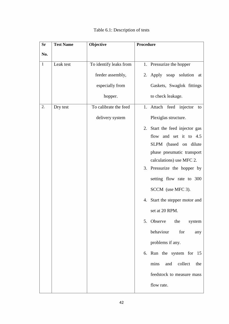
Table 6.1: Description of tests

Sr

No.

Test Name Objective Procedure

1 Leak test To identify leaks from

feeder assembly,

especially from

hopper.

1. Pressurize the hopper

2. Apply soap solution at

Gaskets, Swaglok fittings

to check leakage.

2. Dry test To calibrate the feed

delivery system

1. Attach feed injector to

Plexiglas structure.

2. Start the feed injector gas

flow and set it to 4.5

SLPM (based on dilute

phase pneumatic transport

calculations) use MFC 2.

3. Pressurize the hopper by

setting flow rate to 300

SCCM (use MFC 3).

4. Start the stepper motor and

set at 20 RPM.

5. Observe the system

behaviour for any

problems if any.

6. Run the system for 15

mins and collect the

feedstock to measure mass

flow rate.

43

7. Repeat the procedure upto

30 RPM in steps of

1RPM.(i.e, 20,21,22 etc)

8. Carry out 3 repetitions for

each RPM.

3. Water column

test

To observe if

calibration obtained in

test 2 changes by the

presence of hydrostatic

head

1. Repeat steps 1-3 from test

2.

2. Fill the acrylic column to

desired height to produce

hydrostatic head of 2.9kPa

(this is same as that of

produced by salt in the

reactor.

3. Repeat steps 4-8 from

test#2.

4. High

temperature dry

test

To investigate if

heated feed injector

causes clogging of

feedstock.

1. Wrap tape heater around

feed injector and joint

between screw inlet and

feed injector.

2. Set the voltage such that

temperature of 473K is

achieved on feed injector

surface.

3. Monitor temperature

continuously.

44

4. DO NOT attach acrylic

column to feed injector.

5. Repeat steps 2-3 from test

2.

6. Vary the RPM form 20 to

30 in steps of 1.

7. Run the system for

sufficient time (20-25

mins) to see if heated feed

injector causes any

clogging of feedstock.

8. Collect feedstock ejected

out of feed injector in a

pan.

6.2 Results of Tests

Results are summarized in table 6.2

45

Table 6.2: Results of tests

Sr No. Test Name Results

1 Leak test Feed system could be

pressurized to 7 psig.

2 Dry Test Calibration results given in

section 6.3

3 Water column test Water did not flow back to

the feed injector

4 High temperature dry test No clogging observed

6.3 Calibration of the System

To accurately feedstock into the reactor, calibration of the screw feeder is carried

out. During the calibration, the RPM of the screw was varied and at each RPM the

mass of feed particles collected over the duration of 15 minutes is weighed to

calculate the mass flow rate as a function of RPM. Three measurements were taken at

each and the average value of mass flow rate is presented in the graph shown in figure

6.2. Measurements for mass flow rate are presented in table 6.3.

46

Fig 6.2: Calibration of the feed system

6.4 Uncertainty Analysis

Figure 6.1 shows the calibration graph for feed delivery system. Experimental

data points as well as best linear fit line is shown. The upper and lower confidence

intervals (CI+ and CI- respectively) are shown with the dotted line. Uncertainty in the

data is calculated using LINEST function in Excel. It gives SEE (Standard Error of

Estimate) which is a statistical measure of how well the best-fit line represents the

data. This is, effectively, the standard deviation of the differences between the data

points and the best-fit line. It provides an estimation of the scatter/random error in the

data about the fitted line.

(6.1) 18.02

)(

2/1

2

,

N

yy

SEE

predcitedii

(6.2) 20.0/),(%)95( NSEEtyCI

8

9

10

11

12

13

14

15

20 22 24 26 28

m, (

gm/m

in)

ω,RPM

CI+

CI-

avg. data

Linear (avg. data)

47

2bintercept,in ty Uncertaini

0.07mslope,in ty Uncertaini

Taking into account the uncertainties in slope and intercept, we get

CI 95% ; )232.7()07.079.0(.

RPMm feed

Table 6.3: Calibration of the screw feeder

RPM

Reading 1

(gm/min)

Reading 2

(gm/min)

Reading 3

(gm/min)

Average

(gm/min)

20 8.375 8.421 8.392 8.396

21 9.184 9.234 9.192 9.203

22 10.256 10.288 10.274 10.273

23 10.943 11.232 11.022 11.066

25 12.058 12.344 12.203 12.202

26 13.277 13.657 13.392 13.442

27 13.967 14.213 14.023 14.068

28 14.54 14.992 14.712 14.748

6.5 Reactor Testing

Once the feed delivery system was successfully tested using the tests described

in section 6.2, it was tested with the reactor. For the reactor test, hopper was filled

with an initial mass of 599.5g of cellulose powder. The reactor was heated up to 1150

K using solar simulator with a flow of 3.6 SLPM of nitrogen through the feed

injector. Once molten salt reached 1150 K (monitored using Labview with type-K

TC), CO2 flow (gasifying agent) of 2 SLPM was turned on into the feed injector in

addition to the N2 (for pneumatic transport of feed particles) flow. The feed delivery

system was turned on with the stepper motor being assigned a rotational velocity of

48

18 rpm. At this time the injector temperature was at a temperature of 98oC, and it

varied between 98oC and 95

oC throughout the run time. The big pressure spike

occurred six minutes after the feed was initiated, after which the feed seized up in the

feedscrew shaft.

After the test run was over, the feed system was taken apart and it was found

that the feed injector was actually not blocked in the vertical passage, but it was

blocked in the side passage where the feedscrew comes in. The final mass of cellulose

remaining in the hopper and feedscrew was 557.6g.

Based on the Labview data, it looks like the rising pressure in the reactor (due

to the filters loading up with char/tar) caused the feed injector flow of N2 to decrease

to the point that entrainment of the feed particles was no longer possible. If N2 flow

going through the feed injector was not decreased, the feed system would have

continued to run fine.

49

Chapter 7

Labview Control Scheme

7.1 Objective

Real time sensor output monitoring is very important during a test run. It

enables the user to identify anomalous behavior if any. Also output from sensors

needs to be continuously logged to a file in order to do the post processing of the data.

Mass Flow Controllers (MFCs) need input signal from user to allow the required

amount of gas flow through it. A Labview program is written in order to achieve

above mentioned utilities. It communicates between different sensors and a computer.

It also sends the input signal to the MFCs as given by the user. Table 7.1 lists various

sensors and associated Labview program activity. The location of various sensors is

shown in figure 7.2.

Table 7.1 Sensors and related Labview activity.

Sensor # of

sensors

Labview activity

Type K thermocouple 12 1. To monitor temperatures in realtime.

2. To record temperature data into a file

Absolute pressure sensor 2 1. To monitor inlet and outlet reactor pressures

in realtime.

2. To record pressure data into a file.

Mass Flow Controller

(MFC)

3 1. To set a setpoint for MFC.

2. To monitor the return signal continuously

from MFC.

3. To record flow rates of gases into a file.

50

Figure 7.1 Location of sensors on reactor assembly

7.2 Implementation

The Labview VI written has a front panel and block diagram. Front panel is GUI

which lets the user monitor the real time output of various sensors. Block diagram has

the code which is the functional unit of the VI. Front panel and block diagram are

represented in fig 7.2 and fig 7.3 respectively.

51

Figure 7.2 Front panel of Labview

Fig 7.3: Block diagram of the Labview

52

8. Conclusions and Recommendations for Further Study

8.1 Conclusion

The present study focuses on design, fabrication and calibration of a feedstock

delivery system for a 3kW prototype solar gasification reactor. The primary objective

of the study was to fabricate a feed delivery system capable of delivering 8±(0.4)

gm/min to 15±(0.75) gm/min. of cellulose powder to a gasification reactor. The most

challenging aspect of the study was to select a proper conveying device. Since

commercial augers are made mostly in large sizes (>2” diameter) and are not

available in the small size that was determined taking into the required volumetric

flow rate of feed material, a simple deep drill wood bit was selected as a screw feeder.

Another challenging part of the study was to design a feed injector. The opening of

the flow passage in the feed injector was optimized after taking into account the feed

particle size and manufacturing feasibility. Large flow passage, although would be

required for considerably larger feed particles or any foreign particle of abnormally

large size, but it would have decreased the thermal efficiency of the reactor due to

large flow of N2 going to the reactor.

Testing was carried out to produce calibration of feed mass flow rate vs RPM

of stepper motor. Overall, no overtorque condition or clogging was observed. Also

repeatability was observed in terms of feed delivery rate as a function of RPM of the

stepper motor. Calibration resulted in

During the test of the feed delivery with the reactor, feed particles were

delivered to the reactor for six minutes of time window. However, after that the

pressure built up in the reactor due to the filters loading up with char. It caused the

feed injector flow of N2 to decrease to the point that entrainment of feed particles was

no longer possible.

CI. 95% ; )232.7()07.079.0(.

RPMm feed

53

8.2 Recommendations for further study

The present experimental study mainly focuses on the cellulose particles as a

feedstock which has a particle size of 0.5 mm. The design of various components of

the feed system is done taking into account the size and mechanical properties of the

cellulose particles. Although the change of feed material will not affect the hopper

design that much, it will affect the feed injector flow passage area. Thus current feed

delivery system is restricted to feed material with particle size about 0.5 mm or less.

The stepper motor selected for the present study is based on torque requirement which

depends upon the feed material mechanical properties and feed mass flow rate.

Change of feed material might cause reconsideration for sizing the stepper motor.

This issue can be addressed by replacing current stepper motor (NEMA size 23) by

oversized stepper motor (NEMA size 34) which can be used for variety of feed

material. To prevent the clogging of the feed material, screw feeder tube was cooled

using air jet impingement. Although this method is effective, a better way could be

water jacketing screw feeder tube.

The current feed delivery system does not provide any indication of level

of feedstock in the hopper when experiment is going on. This can be improved by

incorporating an acrylic window slot in the hopper wall to indicate the level of

feedstock. Also to ensure that stepper motor is rotating at set RPM, an encoder can be

employed to track the rotations of the stepper motor.

54

References

[1] Hathaway, B. J., 2013, “Solar Gasification of Biomass”, Ph.D. thesis,

Department of Mechanical Engineering, University of Minnesota.

[2] Dai, J., 2007, “Biomass Granular Feeding for Gasification and Combustion”,

Ph.D. thesis, Department of Mechanical Engineering, University of British

Columbia.

[3] Zareiforoush, H., Komarizadeh, M. H., Alizadeh,M. R., and Masoomi, M.,

“Screw Conveyer Power and Throughput Analysis During Horizontal Handling

of Paddy Grains”, Journal of Agricultural Science,2(2),pp. 1.

[4] Srivastava, A. K., Goering, C. E., Rohrbach, R. P., and Buckmaster, D. R.,

2006, Engineering Principles of Agricultural Machines, Second Edition,

ASABE, pp: 491-524.

[5] Structure of a screw conveyer. Retrieved from:

http://toritdust.com/parts/auger_conveyors.htm.

[6] Types of flights. Retrieved from: http://www.kaseconveyors.com/bulk-

material-handling-products/engineering-guide/conveyor-flight-pitch-types.htm.

[7] Colijn, H., 1985, Mechanical Conveyers for Bulk Solids, Elsevier, New York,

NY, Chap. 3.

[8] Gravity Flow of Bulk Solids, 1964, University of Utah Engineering Experiment

Station, Bulletin 108.

[9] Chase, G. G., 2004, SOLIDS NOTES 10, The University of Akron.

[10] Rhodes, M., 1998, Introduction to Particle Technology, John Wiley and Sons,

West Sussex, England, Chap.10.

[11] Roberts, A.W., 2002, “Design considerations and performance evaluation of

screw conveyors”, Bulk Solids Handling, 22, pp. 436-444.

55

[12] Schematic of deep hole drill bit. Retrieved from:

http://www.mcmaster.com/#drill-bits-for-wood/=nhwvij.

[13] Torque vs speed characteristics for NI NEMA 23 stepper motor. Retrieved

from: http://sine.ni.com/ds/app/doc/p/id/ds-311/lang/en.

[14] Rhodes, M., 1998, Introduction to Particle Technology, John Wiley and Sons,

West Sussex, England, Chap.8.

[15] Arastoopour, H., Modi, M.V., Punwani, D.V., Talwalkar, A.T., 1979

“Review of design equations for dilute phase gas-solids horizontal conveying

systems for coal and related materials”, The Power and Bulk Solids Conference.

[16] Kays, W. M., Crawford, M. E., and Weigand, B., 2004, Convective Heat and

Mass Transfer, 4th ed., McGraw-Hill.

[17] Incropera, F. P., and DeWitt, D. P., 2007, Fundamentals of Heat and Mass

Transfer, John Wiley and Sons, pp.557.

[18] Internal friction data for various materials. Retrieved from:

http://www.stanford.edu/~tyzhu/resources.htm

[19] Beverloo, W. A., Leniger, H.A., Van de Velde, J., 1961 “The Flow of Granular

Solids Through Orifices”, Chem Eng Sci, 115, pp. 260-269.

56

Appendix A

EES code to obtain volume flow rate of nitrogen gas in feed injector:

EES code

Tgas=100+273

Pgas=101325+27000

TSTP=273

rhog=density('Nitrogen',T=Tgas,p=Pgas)

rhop=1200

D=0.12*2.54/100

D_tube=0.18*2.54/100

A_tube=3.14*0.25*D_tube^2

A_tube*V_tube=A*Usafe

L_tube=72*2.54/100

g=9.8

mu=viscosity('N2',T=Tgas)

Mp=15/60/1000

A=3.14*0.25*D^2

Gp=Mp/A

Ut=(2*rp)^2*(rhop-rhog)*g/(18*mu)

((Uch/e)-Ut)=Gp/(rhop*(1-e))

rhog^(0.77)=2250*D*(e^(-4.7)-1)/((Uch/e)-Ut)^2

Usafe=1.5*Uch

VolumeSTP=1000*60*A*Uch*TSTP/Tgas

safeVolume=1.5*VolumeSTP

Uf=Usafe/e

Up=(Mp/rhop)/(A*(1-e))

//Pressure drop calculation

F_fw=(4*tau_w*L/D)

57

(c_f)/2=0.023*Re^(-0.2)

c_f=(tau_w)/(0.5*rhog*Uf^2)

Re=rhog*Uf*D/mu

L=80/1000

F_pw=0.057*Gp*L*(g/D)^0.5

T1=0.5*rhog*e*Uf^2

T2=0.5*(1-e)*rhop*Up^2

T3=F_fw*L

T4=F_pw*L

T5=rhop*L*(1-e)*g

T6=rhog*L*e*g

delta_P=T1+T2+T3+T4+T5+T6

Pressuredrop =delta_P

// Pressure head

// Change Ps by supply line pressure-pressure drop in the line from

gas cylinder to feed injector

Ps=101325

P_dyn=Pgas*(0.028*0.5*Uf^2)/(8.314*Tgas)

P_total=Ps+P_dyn

P_ratio=P_dyn/P_total

// Pressure drop in supply line

F_fw_tube=(4*tau_wtube*L_tube/D_tube)

(c_ftube)/2=0.023*Re_tube^(-0.2)

58

c_ftube=(tau_wtube)/(0.5*rhog*V_tube^2)

Re_tube=rhog*V_tube*D_tube/mu

T1_tube=0.5*rhog*V_tube^2

T3_tube=F_fw_tube*L_tube

T6_tube=rhog*L_tube*g

delta_P_tube=T1_tube+T3_tube+T6_tube

Pressuredrop_total=delta_P_tube+delta_P

// Friction factor asumption

// flow in tube is laminar based on Reynolds number criteria

f=64/Re_tube

deltaP_friction =f*(L_tube/D_tube)*(0.5*rhog*V_tube^2)

59

Appendix B

Standard Operating Procedure (SOP) for feedstock delivery system

Follow the steps in the given order:

Initial system check:

1. for gas system

Check N2 cylinder for sufficient N2 quantity (300 psig) as per required test

run time.

Ensure gas lines connecting to MFC are leak free and located such that it can

NOT be obstructed due to someone stepping over.

Ensure same for gas lines connecting from MFC to hopper and feed injector.

2. Electronics and Power supply

Make sure that there will not be any power shut down during test run.

The computer used for running NI MAX (package for stepper motor) is

working. Deactivate auto sleep/power saver mode of PC

All wires connecting from stepper drive to stepper motor are intact and well

insulated.

Thermocouples monitoring the temperatures of feed injector and screw tubing

are intact.

3. Clogging check

Check screw feeder and hopper thoroughly for any residual clogging from last

run.

Thoroughly clean the screw and screw tubing so that no residual feedstock is

left from last test run.

4. Assembly check

60

Once screw tubing is checked for residual feedstock, assemble the system and ensure

that required protrusion of screw into feed injector opening. (This can be checked by

holding lit torch below feed injector and seeing the protrusion)

The coupling screws should be tightly held on motor shaft and screw shaft to

prevent relative slippage between two shafts.

Load the hopper with required quantity of feedstock.

5. Leak Check

Ensure that all tube fitting connections are tight and leak free.

Also once the hopper is loaded with feedstock, ensure that gasket is in place

and all screws are tight to maintain pressurized hopper.

Check for the bearing for any leaks.

Once above mentioned criteria are checked, you can now proceed with starting the

system.

1. Start cooling system (air jets) to feed injector

2. Start Feed injector gas flow (4.2 SLPM which corresponds to 2.2 V signal

input to MFC2) and then hopper gas flow (200 ccm).

3. Start the NI MAX program to start stepper motor.

4. Check the direction of rotation of stepper motor to ensure forward feeding into

reactor. If direction is reverse, either power off stepper motor system and

interchange A+ and A- on stepper drive then plug in or set the target position

to 9999999. Forward direction can be ensured by looking at the velocity

indicator on MAX. If it shows positive number, it means direction is correct.

5. Monitor the temperatures continuously along screw tubing once preheating of

the reactor is started using tape heaters and ensure that compressed air jet flow

is sufficient to keep the joint between feed injector and screw tubing is just

61

above saturation temperature for steam and temperature of screw tubing

directly below hopper is maintained sufficiently cooler.

6. Start stepper motor by setting at 22 RPM (obtained from calibration) and solar

simulator at the same time For 11 gm/min of feed delivery rate, set RPM of

stepper motor to 22 and acceleration and deceleration to 5 rps/s.

7. When above steps are implanted, feed system is delivering feedstock to the

reactor at required mass flow rate.

Stopping the feedstock system:

When required amount of test run is done, the feedstock delivery system needs to be

stopped.

1. Decelerate stepper motor using NI MAX program to stop it.

2. Increased the compressed air jet flow rate at joint to bring down its temperature

rapidly to near room temperature. If this is not done, residual feedstock in tube

near joint will start clogging. Although this is not a serious problem, but it means

more cleaning will be required for preparing feedstock delivery system for next

text run.

3. Do not stop the N2 supply to feed injector and hopper until molten salt is

drained out from reactor and leftover salt in rector is at a temperature lower than

its melting point.

4. Once the system is cooled completely, open the hopper and remove any leftover

feedstock.

62

Appendix C

Failure modes

Introduction:

Failure Mode Analysis (FMA) has been carried out for various components of the feedstock

delivery system. It briefly describes the failure modes possible for each component along with

its potential cause and possible effects. FMA enables user to foresee any possible failure

based on observation/ sensors output (as described below. It also suggests the remedial

measures so that failed component can be fixed.

Table C.1: Failure modes

Component Failure mode Possible

Effects

Potential causes Fix

Feedscrew 1.Solid

feedstock clogs

inlet passage

2.Char/tar clogs

inlet passage

3.Loss of gas

flow

Feeding stops.

Salt temperature

begins to rise.

Salt backflow

into feed

injector. Line

pressure

upstream of

clog begins to

rise.

Feeding stops.

Salt temperature

begins to rise.

Salt backflow

into feed

injector. Line

pressure

upstream of

Excessive feed

rate. Insufficient

gas to feed rate.

Excessive

Injector

temperature.

Excessive solid

residence time in

injector.

Slow feedstock

delivery rate.

Increase vertical

injection path

diameter

Increase cooling

of injector body

Ensure

sufficient

63

clog begins to

rise.

Feedstock fills

injector body

and feeding

stops. Salt

backflow into

feed injector.

Insufficient gas

supply line

pressure.

Insufficient gas

flow setpoint

applied to MFC.

nitrogen

available before

experiment.

Feedscrew Loss of feed

flow

Salt temperature

begins to rise.

Stepper motor

failure or

overtorque

condition.

Feedstock in

solid rotation

with shaft (no

feeding).Motor

to screw shaft to

coupling failure.

Labview freezes.

Check stepper

motor wiring.

Increase motor

size if required.

Switch from

auger based to

helical spring

based feeding.

Make sure that

coupling screws

are tight so that

there is no

relative motion

between motor

shaft and screw

shaft.

Hopper Feedstock

bridging over

feedscrew.

Loss of gas seal

Loss of feed

flow as

described above

Backflow of gas

from injector.

Inability to

carry feed into

Feedstock too

moist. Hopper

walls too flat

Bearing seal

failure. Tube

fitting seal

failure. Hopper

Add hopper

vibration.

Consider further

drying

feedstock. Make

sure that sight

glass is clean

Perform leak

checks. Replace

failed seals.

Consider new

64

Loss of

pressurization

reactor.

Potential

clogging of

injector.

Potential

backflow of salt

from rector to

injector.

Backflow of gas

from injector.

Inability to

carry feed into

reactor.

Potential

clogging of

injector.

Potential

backflow of salt

from rector to

injector.

window seal

failure. Hopper

to tube welds

failure.

Insufficient gas

supply pressure.

Insufficient gas

flow setpoint for

MFC.

fitting or shaft

bearing

arrangement.

Ensure

sufficient

nitrogen is

available before

testing. Ensure

emergency air

divergence

valve available

in case of loss of

nitrogen supply.

Check MFC

setpoint.