Embed Size (px)
Citation preview

CHAPTER 2
Derivation of Kinetic Equations
As we said, the mathematical object that we consider in Kinetic Theoryis the distribution function 0 f(t, x, v). We will now be a bit moreprecise about the link between microscopic and mesoscopic descriptions ofa system. Consider a gas (or more generally a system) of N particles (ormore generally bodies) indistinguable, and in particular of the same massm = 1. For now for simplification we will consider them to be point particles(i.e. zero volume), an assumption that we will come back to later.
1. Newtonian Viewpoint
We assume some binary interaction through a potential , dependingonly on the distance between two interacting bodies and in addition anexternal force with some potential �(t, position). If we label each particlewith an index 1 i N , and call the i-th particle’s position xi and velocityvi, then Hamiltonian’s formulation of Newtonian mechanics gives us (recallthat the masses of particles are normalized to one) that
(1.1)dxi
dt=@H
@vi
dvidt
= �@H@xi
where
H =NX
i=1
v2i2
| {z }kinetic energy
+X
i<j
(xi � xj)
| {z }interaction energy
+NX
i=1
�(t, xi).
| {z }potential energy
This corresponds to the following ODE’s
8 1 i N, xi = vi, vi = �X
i 6=j
rx (xi � xj)�rx�(xi).
For now, we are assuming that and � are “regular” i.e. su�cientlysmooth to ignore any reasonable di↵erentiability/convergence issue.
As a general convention in the sequel:
15

16 2. DERIVATION OF KINETIC EQUATIONS
• Note that when we write a vector on the bottom of the derivative,it really means the directional derivative in that direction.
• Lowercase letters refer to one i-th particle whereas uppercase let-ters refer to the vector of all particles X = (x
1
, . . . , xN) and V =(v
1
, . . . , vd). If each xi 2 R3, this is actually a vector of vector(matrix).
Discuss the signs of the di↵erent part of the energy functional.
2. The notion of dynamical system (S)
Here introduce the hamiltonian formulation, and some key elementaryproperties.
Exercise 2. Define for any t 2 RS(t) : (Rd ⇥ Rd)N ! (Rd ⇥ Rd)N , (X, V ) 7! St(X, V ) = (Xt, Vt)
given by the evolution (1.1) between time 0 and t. Prove that (1) H isconstant along S, and (2) S(t) has Jacobian 1 for a fixed t (this is one formof the Liouville theorem).
3. Statistical Viewpoint
3.1. The N-body Liouville equation. Now, instead of consideringthe above microscopic viewpoint of the trajectories, we will shift to a morestatistical viewpoint. As such, we consider a joint distribution function forall of the particles FN(t,X, V ). We claim that FN evolves as such:
(3.1)@FN
@t+
NX
i=1
✓@H
@vi· @FN
@xi� @H
@xi· @FN
@vi
◆= 0
We shall call this equation the N-particle Liouville equation. Let us explainheuristically how we derived (i.e. “guessed”) from the ODE’s defining thetrajectories. Since we want an equation on the distribution function ofparticles, it is clear that this distribution should be preserved when followingthe trajectories of each particle:
8 t � 0, F (t, St(X, V )) = F (0, X, V ).
In other words, we consider the distribution of particles following theirtrajectories. FIGURE TO BE ADDED HERE
Let us now di↵erentiate in time the equation with the help of the chain-rule (assuming that every terms are smooth):
4. THE CHARACTERISTICS METHOD (S) 17
✓@
@tF
◆(t,Xt, Vt) +
✓@
@tXt
◆·✓
@
@XF
◆(t,Xt, Vt)
+
✓@
@tVt
◆·✓@
@VF
◆(t,Xt, Vt) = 0
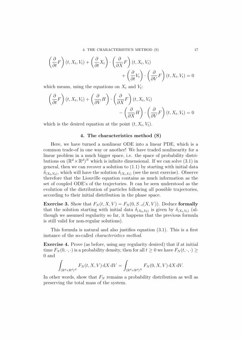
which means, using the equations on Xt and Vt:✓@
@tF
◆(t,Xt, Vt) +
✓@
@VH
◆·✓
@
@XF
◆(t,Xt, Vt)
�✓
@
@XH
◆·✓@
@VF
◆(t,Xt, Vt) = 0
which is the desired equation at the point (t,Xt, Vt).
4. The characteristics method (S)
Here, we have turned a nonlinear ODE into a linear PDE, which is acommon trade-of in one way or another! We have traded nonlinearity for alinear problem in a much bigger space, i.e. the space of probability distri-butions on (Rd⇥Rd)N which is infinite dimensional. If we can solve (3.1) ingeneral, then we can recover a solution to (1.1) by starting with initial data�(X0,V0), which will have the solution �
(Xt
,Vt
)
(see the next exercise). Observetherefore that the Liouville equation contains as much information as theset of coupled ODE’s of the trajectories. It can be seen understood as theevolution of the distribution of particles following all possible trajectories,according to their initial distribution in the phase space.
Exercise 3. Show that FN(t,X, V ) = FN(0, S�t(X, V )). Deduce formallythat the solution starting with initial data �
(X0,V0) is given by �(X
t
,Vt
)
(al-though we assumed regularity so far, it happens that the previous formulais still valid for non-regular solutions).
This formula is natural and also justifies equation (3.1). This is a firstinstance of the so-called characteristics method.
Exercise 4. Prove (as before, using any regularity desired) that if at initialtime FN(0, ·, ·) is a probability density, then for all t � 0 we have FN(t, ·, ·) �0 and ˆ
(Rd⇥Rd
)
N
FN(t,X, V ) dX dV =
ˆ(Rd⇥Rd
)
N
FN(0, X, V ) dX dV.
In other words, show that FN remains a probability distribution as well aspreserving the total mass of the system.

18 2. DERIVATION OF KINETIC EQUATIONS
Explain how the Liouville theorem translates in this statistical view-point.
5. The many-particle limit
5.1. The One Particle Distribution. Observe that the N -particleLiouville equation, although it allows for considering superpositions of alltrajectories at the same time, still contains exactly the same amount ofinformation as the original Newton equations. And in most situations thisis much more that we need, want and can experimentally measure (do notforget we have to enter initial data in our equation for it to be useful!).
We will now simplify our description of the system by throwing awayinformation. (Hopefully) the system is described by a “one particle distri-bution,” i.e. a typical distribution of one particle, for which we can obtaina distribution from FN by taking the first marginal:
f(t, x, v) :=
ˆ(Rd⇥Rd
)
N�1
FN(t,X, V )dx2
dx3
, . . . dxN dv2
. . . dvN .
Why the marginal according to the first variable without loss of general-ity? We consider FN to be symmetric under permutations of the particle’sindexes due to the indistinguability of the particles, so choosing i = 1 isnot important, as we would obtain the same answer for any other choice ofindex.
How can we obtain an equation for how f evolves? The natural thing todo is of course to integrate (3.1) in the x
2
, v2
, . . . , xN , vN variables. For no-tational simplicity we write X(1) = (x
2
, x3
, . . . , xN) 2 Rd(N�1) and similarlyfor V (1).
The first term in (3.1) isˆ(Rd⇥Rd
)
N�1
@FN
@tdX(1) dV (1) =
@
@t
ˆ(Rd⇥Rd
)
N�1
FN dX(1) dV (1)
�=@f
@t.
The integral of the second term in (3.1) is the sum over i ofˆ(Rd⇥Rd
)
N�1
@H
@vi· @FN
@xidX(1) dV (1)
=
ˆ(Rd⇥Rd
)
N�1
vi@FN
@xidX(1) dV (1)
=
ˆ(Rd
)
N�1
vi
✓ˆ(Rd
)
N�1
@FN
@xidX(1)
◆dV (1) =
8><
>:
v1
@f
@x1
i = 1
0 i � 2.
5. THE MANY-PARTICLE LIMIT 19
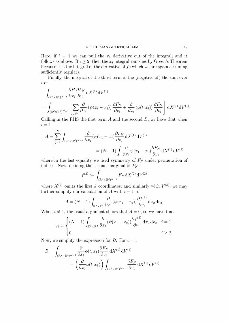
Here, if i = 1 we can pull the x1
derivative out of the integral, and itfollows as above. If i � 2, then the xi integral vanishes by Green’s Theorembecause it is the integral of the derivative of f (which we are again assumingsu�ciently regular).
Finally, the integral of the third term is the (negative of) the sum overi ofˆ
(Rd⇥Rd
)
N�1
@H
@xi
@FN
@vidX(1) dV (1)
=
ˆ(Rd⇥Rd
)
N�1
"X
j 6=i
@
@xi( (xi � xj))
@FN
@vi+
@
@xi(�(t, xi))
@FN
@vi
#dX(1) dV (1).
Calling in the RHS the first term A and the second B, we have that wheni = 1
A =NX
j=2
ˆ(Rd⇥Rd
)
N�1
@
@x1
( (x1
� xj)@FN
@v1
dX(1) dV (1)
= (N � 1)
ˆ@
@x1
(x1
� x2
)@FN
@v1
dX(1) dV (1)
where in the last equality we used symmetry of FN under permutation ofindices. Now, defining the second marginal of FN
f (2) :=
ˆ(Rd⇥Rd
)
N�2
FN dX(2) dV (2)
where X(k) omits the first k coordinates, and similarly with V (k), we mayfurther simplify our calculation of A with i = 1 to
A = (N � 1)
ˆRd⇥Rd
@
@x1
( (x1
� x2
))@f (2)
@v1
dx2
dv2
.
When i 6= 1, the usual argument shows that A = 0, so we have that
A =
8><
>:
(N � 1)
ˆRd⇥Rd
@
@x1
( (x1
� x2
))@f (2)
@v1
dx2
dv2
i = 1
0 i � 2.
Now, we simplify the expression for B. For i = 1
B =
ˆ(Rd⇥Rd
)
N�1
@
@x1
�(t, x1
)@FN
@v1
dX(1) dV (1)
=
✓@
@x1
�(t, x1
)
◆ˆ(Rd⇥Rd
)
N�1
@FN
@v1
dX(1) dV (1)

20 2. DERIVATION OF KINETIC EQUATIONS
=
✓@
@x1
�(t, x1
)
◆@
@v1
✓ˆ(Rd⇥Rd
)
N�1
FN dX(1) dV (1)
◆=
@�
@x1
@f
@v1
.
Thus
B =
8><
>:
@�
@x1
@f
@v1
i = 1
0 i � 2.
Thus, combining these into our integrated (3.1) gives the equation forthe one marginal distribution(5.1)
@f
@t+ v
@f
@x� @�
@x
@f
@v� (N � 1)
ˆ@
@x( (x� y))
@f (2)
@v(x, y, v, w)dydw = 0
(where we have made the substitutions x1
! x, x2
! y, v1
! v, v2
! w).How can we interpret this equation? Binary collisions mean that the
evolution of the first marginal (f) depends on the second one. Similarlywe could show that f (2)’s evolution depends on f (3) and so on. Doing so,we could write down the “BBGKY hierarchy” (Bogoliubov, Born, Green,Kirkwood, Yvon hierarchy, sometimes called Bogoliubov hierarchy) for
f, f (2), . . . , f (N) = FN .
5.2. The Many-particle or “Thermodynamic” Limit. The goalof the thermodynamical limit is to take N ! 1 and recover an equationfor only the first marginal. The rough idea is that we would very much liketo write
f (2) = f ⌦ f := f(x, v)f(y, w)
in order to get a closed equation on the one particle marginal. This is themost natural guess if the particles are not too much coupled.
However there are two complications:
• This independence assumption is easily seen to be incorrect, pre-cisely due to the interactions in the system which create correla-tions between particles. What Boltzmann understood (and Kac [37]formulated mathematically) was that (maybe) as N ! 1 thiscould be true in some sense:
f (2) ⇠ f ⌦ f as N ! +1.
This is the idea of molecular chaos of Boltzmann.• There should some kind of scaling in the interaction (here repre-sented by the interaction potential ), if not the factor (N � 1)would blow-up in our equation (5.1).

6. MEAN FIELD MODELS 21
In general one has to use more complicated models in which the particleshave non-zero radius r and some assumptions of the form
(1) N � 1 (or even N ! 1).(2) There is a fixed volume V , so because N ! 1 we must also take
r = r(N) ! 0.(3) Some version of molecular chaos.(4) Some way of scaling the interaction, i.e. = N .
Given di↵erent choices in how to make these assumptions we arrive at dif-ferent models. This is how the kinetic equations are derived and obtainedfrom physics, at least formally.
6. Mean Field Models
6.1. The mean-field limit. In this approach, we do not try to de-scribe each binary interaction, but only their collective e↵ect. It is a goodapproach when the interaction potential is “not too sensitive to the pre-cise position of each particle.” Often this assumption is called long rangeinteraction. The extreme opposite case is when there are only contact in-teractions by collisions, like for the case of hard balls / spheres that we shallconsider in the next section.
Mathematically, we let N(z) =1
N (z). We take r = r(N) ! 0 such
that Nr3
V ⌧ 1. In other words, this is an assumption of dilute gas. Noticethat the force between two particles is O(1/N), but there are N � 1 otherparticles, so a particular particle feels a force of O(N�1
N ) = O(1).This model is well adapted to electromagnetic and gravitational forces.
What we hope for is that under these assumptions, following our previouscalculations we could get the following Vlasov equation for f :
(6.1)@f
@t+ v
@f
@x� @�
@x
@f
@v�ˆ
@
@x( (x� y))
@f
@v(x, v)f(y, w)dydw = 0
This equation is obtained from (5.1) by plugging N = /N , using thedecorelation assumption f (2) ⇠ f ⇥ f , and taking the limit N ! +1.
6.2. The main mean-field kinetic PDEs. In the case where thereis no external force � = 0 (this plays no essential role in the discussionhere) and we start microscopically from the Coulomb interaction betweenelectrons
(x� y) =1
|x� y|

22 2. DERIVATION OF KINETIC EQUATIONS
we obtain the Vlasov-Poisson for plasmas (assuming here that the elec-tric charge of an electron is normalized to �1 and normalized all physicalconstants):
@f
@t+ v ·rxf +
F
m·rvf = 0
where F = �E with E the electric field from the other particles, andE = r where (the mean-field potential) satisfies the so-called Poissonequation
� =
⇢ions
�ˆ
f dv
�
| {z }charge density
where ⇢ions
is a fixed density of ions in the plasma. We assume there is nooverall charge, which gives us thatˆ
⇢ions
dx =
ˆf dx dv.
This is the main equation in plasma physics. This force field F is there-fore“self induced” and is responsible for a quadratic nonlinear term in theequation. This nonlinearity results in oscillations in the plasma.
In the case of Newton gravitation forces between stars “microscopically”(assuming that all stars have mass normalized to 1 and normalizing allphysical constants)
(x� y) = � 1
|x� y|we obtain the gravitational Vlasov-Poisson equation, in which f describesthe distribution of starts in the galaxy: F = �E, where again E = r isthe gravitational field from the other stars, and (the mean-field potential)satisfies the Poisson equation
� = ⇢ where ⇢ =
ˆf dv is the local matter density.
Summing up, what we call the Vlasov-Poisson equations are:
(6.2)@f
@t+ v ·rxf + F ·rvf = 0
Plasma: F = �rx �x = ⇢ions
�ˆ
f dv
Galaxies: F = �rx �x =
ˆf dv.
Note that the plasma case is repulsive and the galaxy case is attractive.
6. MEAN FIELD MODELS 23
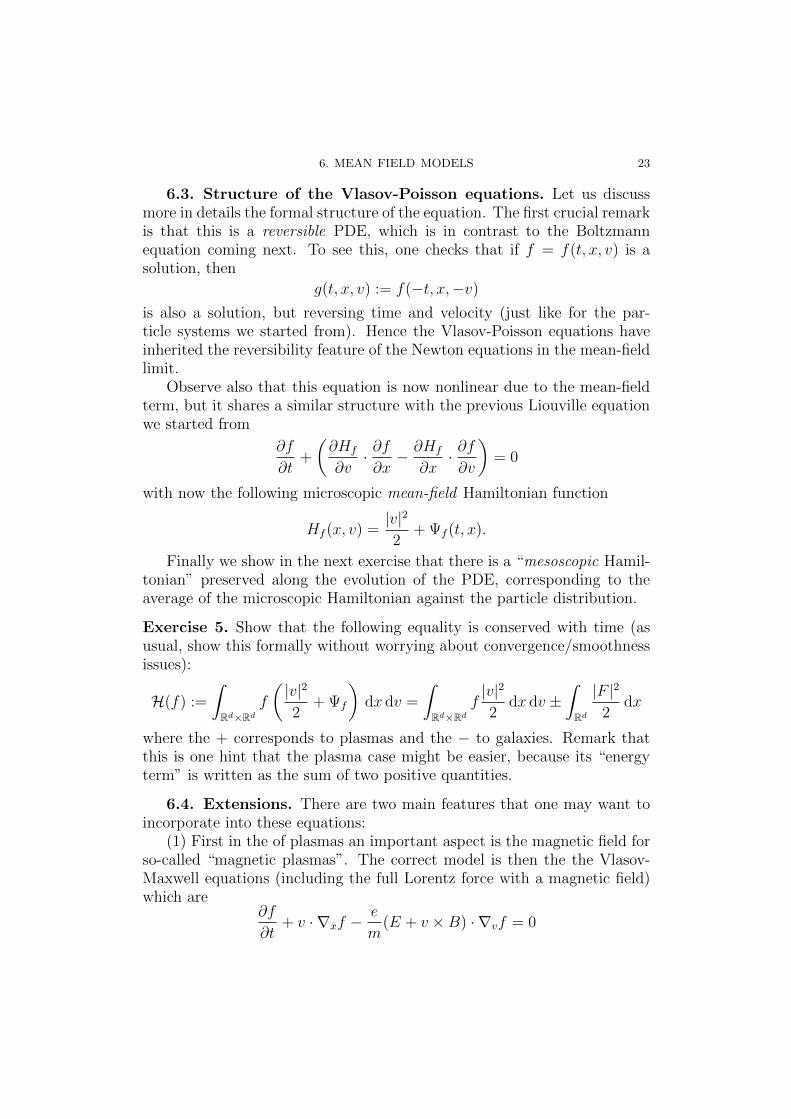
6.3. Structure of the Vlasov-Poisson equations. Let us discussmore in details the formal structure of the equation. The first crucial remarkis that this is a reversible PDE, which is in contrast to the Boltzmannequation coming next. To see this, one checks that if f = f(t, x, v) is asolution, then
g(t, x, v) := f(�t, x,�v)
is also a solution, but reversing time and velocity (just like for the par-ticle systems we started from). Hence the Vlasov-Poisson equations haveinherited the reversibility feature of the Newton equations in the mean-fieldlimit.
Observe also that this equation is now nonlinear due to the mean-fieldterm, but it shares a similar structure with the previous Liouville equationwe started from
@f
@t+
✓@Hf
@v· @f@x
� @Hf
@x· @f@v
◆= 0
with now the following microscopic mean-field Hamiltonian function
Hf (x, v) =|v|22
+ f (t, x).
Finally we show in the next exercise that there is a “mesoscopic Hamil-tonian” preserved along the evolution of the PDE, corresponding to theaverage of the microscopic Hamiltonian against the particle distribution.
Exercise 5. Show that the following equality is conserved with time (asusual, show this formally without worrying about convergence/smoothnessissues):
H(f) :=
ˆRd⇥Rd
f
✓ |v|22
+ f
◆dx dv =
ˆRd⇥Rd
f|v|22
dx dv ±ˆRd
|F |22
dx
where the + corresponds to plasmas and the � to galaxies. Remark thatthis is one hint that the plasma case might be easier, because its “energyterm” is written as the sum of two positive quantities.
6.4. Extensions. There are two main features that one may want toincorporate into these equations:
(1) First in the of plasmas an important aspect is the magnetic field forso-called “magnetic plasmas”. The correct model is then the the Vlasov-Maxwell equations (including the full Lorentz force with a magnetic field)which are
@f
@t+ v ·rxf � e
m(E + v ⇥ B) ·rvf = 0
24 2. DERIVATION OF KINETIC EQUATIONS
where E,B satisfy Maxwell’s equations
r · E = ⇢, r · B = 0, r⇥ E = �@tB, rB = J + @tE
with J = cst´vf dv. One could even include special relativity e↵ect which
yields mathematically a compactification of the variable v. Almost no ex-istence/uniqueness results are known for these equations, the best result sofar is the conditionnal result of Glassey and Strauss [26].
(2) Second in the case of gravitational interaction, one may want toincorporate the general relativity and the curved structure of the space-time. This would result in the so-called Vlasov-Einstein, where the Vlasovequations for the transport of matter are coupled with the Einstein equationfor the metric of the space-time structure. There are very few for thisequation as well, we refer to the book [52] by an expert in this field.
7. Boltzmann-Grad Limit and Collisional Models
In contrast to the mean field models, here we consider short range in-teractions. Typically the model is elastic collisions by hard spheres. Noticethat this is extremely sensitive to the position of the particles, i.e. up tothe scale of their size. For example, if two particles of diameter d are adistance d apart, and if they are on a collision course, then moving one ofthem a distance of 2d will make it so that they do not collide.
From the scaling (as N ! 1), requiring the mean free path
`(N) =v1/3
N� r(N)
the radius of the particles, and
Nr(N)2 = O(1) as N ! 1,
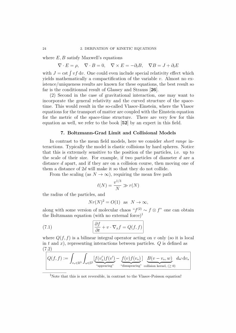
along with some version of molecular chaos “f (2) ⇠ f ⌦ f” one can obtainthe Boltzmann equation (with no external force)1
(7.1)@f
@t+ v ·rxf = Q(f, f)
where Q(f, f) is a bilinear integral operator acting on v only (so it is localin t and x), representing interactions between particles. Q is defined as(7.2)
Q(f, f) :=
ˆv⇤2R3
ˆ!2S2
[f(v0⇤)f(v0)| {z }
“appearing”
� f(v)f(v⇤)| {z }“dissapearing”
] B(v � v⇤, w)| {z }collision kernel, (� 0)
d! dv⇤
1Note that this is not reversible, in contrast to the Vlasov-Poisson equation!

7. BOLTZMANN-GRAD LIMIT AND COLLISIONAL MODELS 25
where
v0 := v � hv � v⇤,!i!v0⇤ := v⇤ + hv � v⇤,!i!
Here, the terms marked “appearing” are there because they represent twoparticles colliding and then having velocities v0⇤ and v0, and similarly with“dissapearing.” We assume that B is “even” in the first coordinate.
Let us only sketch the idea of the formal derivation, which turns out tobe much more complicated than the mean-field limit. We start from the Nparticle Liouville equation
@tFN + V ·rXFN = 0
but which is now posed on the domain
⌦N := {8i 6= j, |xi � xj| � 2r(N)} .We then consider again the one-particle distribution
f(t, x, v) :=
ˆ(Rd⇥Rd
)
N�1
FN(t,X, V ) dx2
dx3
, . . . dxN dv2
. . . dvN
and we search for an evolution equation on it:
@tf + v1
·rx1f = �NX
j=2
ˆX(1),V (1)2⌦(1)
N
vj ·rxj
FN
= �(N � 1)h ˆ
+
f (2)(x1
, x2
, v1
, v2
)|(v1
� v2
) · n12
|d�12
dv2
�ˆ�f (2)(x
1
, x2
, v1
, v2
)|(v1
�v2
)·n12
|d�12
i+ cancelling or negligeable terms
by Green’s theorem, where n12
is the outer normal to the sphere |x1
�x2
| =2r(N), d�
12
is the surface element on the same sphere, and f (2) is as beforethe two-particle distribution, and where
´+
denotes the surface term foroutgoing collisions (v
1
� v2
) · n12
� 0 and´� denotes the surface term for
ingoing collisions (v1
� v2
) · n12
0.We have here
• neglected multiple collisions (more than binary) which have zeromeasure in the limit,
• considered a domain without boundary• use the cancellation of the surface terms not involving x
1
(thanksto the reversibility of the collisions).

26 2. DERIVATION OF KINETIC EQUATIONS
Then in the surface integrals´+
and´� one has to express outgoing
velocities in´+
in terms of the ingoing velocities in´�. This is where
a time arrow is introduced. This choice seems innocent and arbitrary atthe microscopic level but cannot be reversed after the limit N ! +1 hasbeen taken2. Under the previous assumptions (scaling, molecular chaos)we then formally obtain the Boltzmann equation with the collision kernelB(v � v⇤,!) = |(v � v⇤) · !|.Exercise 6. Show that
v0 + v0⇤ = v + v⇤(7.3)
|v0⇤|2 + |v0|2 = |v|2 + |v⇤|2(7.4)
i.e. we can think of this as two particles colliding with initial velocities(v, v⇤) and then leaving with velocities (v0, v0⇤). The above shows us thatwe have energy and momentum conservation (which we expected, becausethis is an elastic collision).
Exercise 7.
(1) For a fixed ! 2 S2 show that the map
(v, v⇤) 7! (v0, v0⇤)
has Jacobian �1.(2) Deduce formally that for a test function �(v)ˆ
Q(f, f)�(v) dv =1
4
ˆv2R3
ˆv⇤2R3
ˆ!2S2
[f 0f 0⇤�ff⇤]B(v�v⇤,!)(�+�⇤��0��0
⇤)d! dv⇤ dv
where the 0 and ⇤ after � and f signify evaluating the function atv0, v⇤ respectively, i.e. f 0
⇤ = f(v0⇤).(3) Given (2), what can you deduce from the following choices of �:
� = 1
� = vi i = 1, 2, 3
� = |v|2� = log f
Note that everything we have done above does not depend on the dimen-sion, so we will refer instead to a general dimension d instead of d = 3 fromnow on. For the integration by parts argument, we used some decay of � atinfinity, in order to integrate by parts, so the assignments �(v) = 1, vi, etc
2The other choice at the microscopic level (expressing pre-collisional velocities interms of post-collisional ones) would lead to a backward Boltzmann equation, with aminus in front of the collision operator.

7. BOLTZMANN-GRAD LIMIT AND COLLISIONAL MODELS 27
might not seem justified, but by multiplying by a cuto↵ function and thenletting it tend to 1, it is not hard to make these arguments more rigorous.
Thus, we have obtained a priori estimates, which we can write compactlyas ˆ
Rd
Q(f, f)
0
@1v|v|2
1
A dv = 0
From the Boltzmann equation (7.1), it is not hard to deduce a priori that
d
dt
ˆRd⇥Rd
f
0
@1v|v|2
1
A dv dx = 0
andd
dtH(f) =
d
dt
ˆRd⇥Rd
f log f dv dx = D(f) 0.
Also, as we remarked above, notice that if we have equality in the en-tropy a priori estimate, i.e. ˆ
Q(f, f) log f = 0
then we have that
(7.5) ff⇤ = f 0f 0⇤
holds. One of the reasons Boltzmann was convinced that his equation wascorrect is that this condition implies that f must be a gaussian.
Exercise 8. If (7.5) holds for f 2 C1c (Rt ⇥ Rd
x ⇥ Rdt ;R), show that f is a
gaussian. (More hints in the example sheet).
As remarked above, there has been few progress on the Cauchy problemfor the full Boltzmann equation, (7.1). Thus, simplified models are some-times studied. For example, the BGK collision model replaces Q(f, f) withMf � f where
Mf =⇢
(2⇡T )d/2e�|v�u|2/2T
is the gaussian with the same parameters v, ⇢ and T as f (as defined in(1.2), (1.1) and (1.3)).
Exercise 9. Check that the “BGK” model satisfies the same formal prop-erties as the original Boltzmann equation (conservation laws, H-theorem).

28 2. DERIVATION OF KINETIC EQUATIONS
8. “A priori estimates” and nonlinear PDEs (S)
Show the naive Gronwall estimate at work on the two previous nonlinearequations, the associated fixed point iteration method (cf. Picard-Lindelof)and its limit for long-time results.
Then explain what is an “a priori estimates” and why it is crucial inorder to go beyond the short-time results obtained by the naive approach.
Then explain the contradiction between controlling the nonlinear termand the controls provided by the known “a priori estimates” given byphysics. Illustrate with VP, BE, but also NS.
9. Bibliographical and historical notes
A large amount of the initial draft version of this chapter is indebted tothe nice lecture notes [54] of Laure Saint-Raymond.
The reformulation of the mechanics of Newton in terms of the (nowcalled) “Hamiltonian canonical forms” was discovered by the irish math-ematician Hamilton in 1833. The so-called “Liouville equation” for theevolution of the probability density in phase space associated to a dynam-ical system goes back to a paper of the french mathematician Liouville of1838, as well as the so-called “Liouville theorem”. The BBGKY hierar-chy obtained from the many-particle Liouville equation was discovered inindependent works published in 1946 and 1947 by Bogoliubov in USSR,Kirkwood in USA, Born in Germany and his former student scottish stu-dent Green.
Concerning the Vlasov-Poisson, there have been important progresses onthe Cauchy problem. As suggested in the introduction, in a “small space”of solutions (with high regularity and decay at infinity) local existence anduniqueness is not too hard and have been proven [2] and global existenceand uniqueness for small initial data [6], but global existence in general hasbeen unknown for a while, while in a “very large space” (like L1 functionssatisfying bounds on the macroscopic Hamiltonian H and the entropy) it ispossible to get global existence [3], but uniqueness is then unknown.
Pfa↵elmoser [51] and then Lions and Perthame [45] showed the exis-tence and uniqueness of global solutions in the all space x 2 Rd. Theirsettings are di↵erent: Pfa↵elmoser assumes that the initial data is Ck
with compact support (thus building classical smooth solutions), and Li-ons and Perthame consider initial data which are L1 with some velocitymoments and some initial mild regularity estimate on the initial density

10. EXERCISES 29
⇢in =´fin dx. However it is hard to make any interesting qualitative ob-
servations about these solutions. These proofs have later been digested,optimized, extended and improved: see [55], [7], [34], [49].
Concerning the mean-field limit and the derivation of the Vlasov-Poisson,only partial progresses have been and the problem remains open for theCoulomb and Newton interactions: we refer to [9] and [22] in the case ofsmooth interactions, and to [31] for a partial result in the case of singularinteractions.
Concerning the Boltzmann equation the situation is much less advanced.There has been only partial progress on the Cauchy problem. For highregularity (i.e. a small space) perturbative solutions (close to equilibriumor close to vacuum) have be built, see for instance [56] and [36]. Forlow regularity, DiPerna and Lions [21] showed in 1989 that there is globalexistence of “renormalized solutions” which is a type of (very) weak solution.However, nothing is known in between these two. With further invarianceswe have better theories: in the case of spatially homogeneous solutions orone-dimensional (in space) solutions.
Concerning the Boltzmann-Grad limit this remains an important openproblem. The best (and by far most important) result so far is due toLanford [41] and proves the limit for a gas of hard spheres but only fora very short time (less than the mean-free time between collisions that aparticle encounters). This theorem has been extended to a global in timelimit theorem in the case of solutions close to vacuum in [35].
Among existing books, two nice references are [25], more oriented to-wards Vlasov equations, and [16], more oriented towards Boltzmann colli-sional equations. In particular the first chapters the latter book explainedin great details the Boltzmann-Grad limit and Lanford’s Theorem.
10. Exercises