Department of Land Economy1 LECTURE 1 EMERGENCE OF NCM Philip Arestis University of Cambridge and University of the Basque Country

Department of Land Economy 1

UNIVERSITY OF

CAMBRIDGE

Department of Land Economy

LECTURE 1

EMERGENCE OF NCM

Philip ArestisUniversity of Cambridge and University of

the Basque Country


LECTURE 1: INTRODUCTION

Circular Flow of Income

Real Sector

Monetary Sector

Foreign Sector

Inflation

Neoclassical Synthesis

New Classical Economics

New Keynesian Economics

New Consensus Macroeconomics



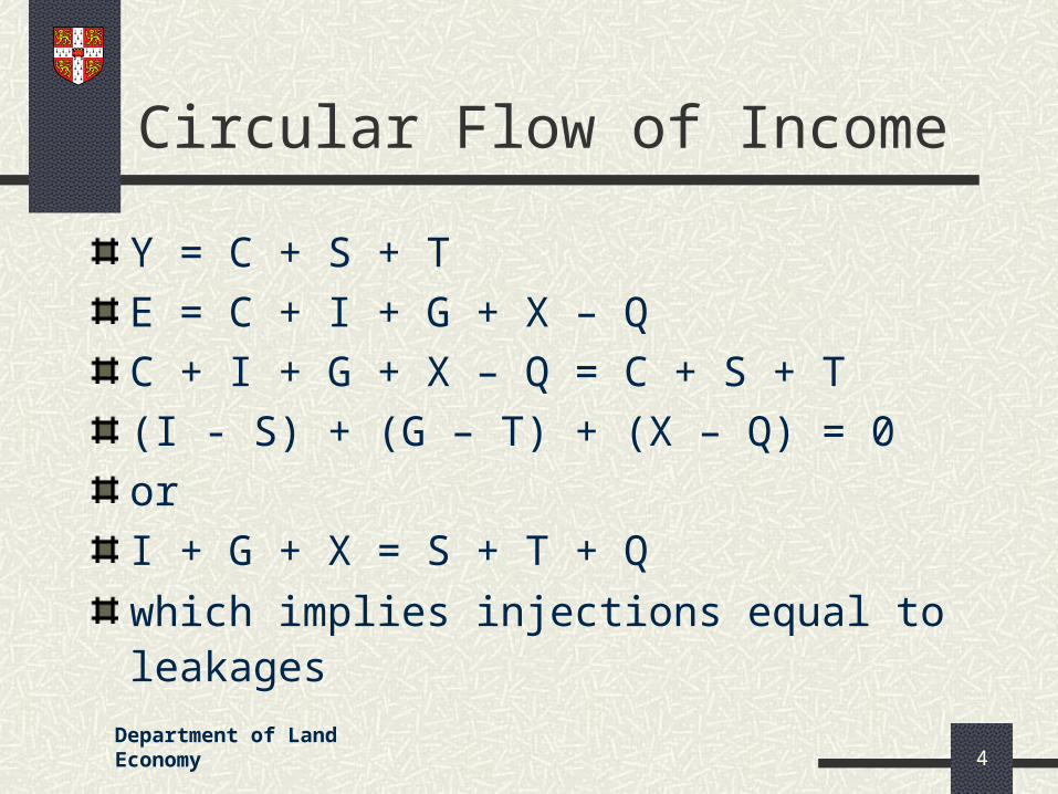
Figure 1: Circular flow of income



Y = C + S + T

E = C + I + G + X – Q

C + I + G + X – Q = C + S + T

(I - S) + (G – T) + (X – Q) = 0

or

I + G + X = S + T + Q

which implies injections equal to leakages



Assuming closed economy:

Y = E = C + I + G

C = c0 + c1YD

with 0 < c1 < 1

Y = c0 + c1(Y – T) + I + G

YD = Y – T

Y = c0 + c1Y – c1T + I + G



Y(1-c1) = c0 – c1T + I + G

Y = [1/(1-c1)].(c0 - c1T + I + G)i.e. the equilibrium level of income And with T and G given, but allowing I to change:

ΔY = [1/(1-c1)]. ΔI or

(ΔY/ ΔI) = 1/(1-c1)i.e. the multiplier.



Figure 2: Equilibrium level of income

Y0 Y1 Y2

E

E2

E1A

BC

D

F

E

E’45O



Equivalently:

Y = C + S + T, or

S = Y – C – T, or

S = C + I + G – C – T, or

S = I + G – T, or

I = S + (T – G)

i.e. investment is equal to the total of savings.



We may use the model:

Y = E = C + I + G

C = c0 + c1YD

YD = Y – T

I = i0 + i1r

where we treat G and T still as exogenous, but

I is treated now endogenous, with i1<0. We can

have:



Y = c0 + c1(Y - T) + i0 + i1r + G

Y - c1Y = c0 - c1T + i0 + G + i1r

Y(1 - c1) = c0 - c1T + i0 + G + i1r

Y = [1/(1-c1)].(c0 + i0 - c1T + G)

+ [i1/(1-c1)].r

We explain this relationship in Figure 3:



Figure 3: The IS relationship

Y0 Y1 Y2

E

E

E’45O

IS

Yo

Y0 Y1 Y2

E’’

r2

r1

r0


Real Sector

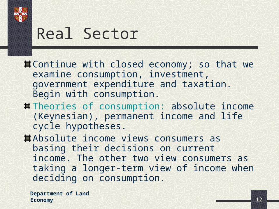
Continue with closed economy; so that we examine consumption, investment, government expenditure and taxation. Begin with consumption.Theories of consumption: absolute income (Keynesian), permanent income and life cycle hypotheses.Absolute income views consumers as basing their decisions on current income. The other two view consumers as taking a longer-term view of income when deciding on consumption.


Real Sector

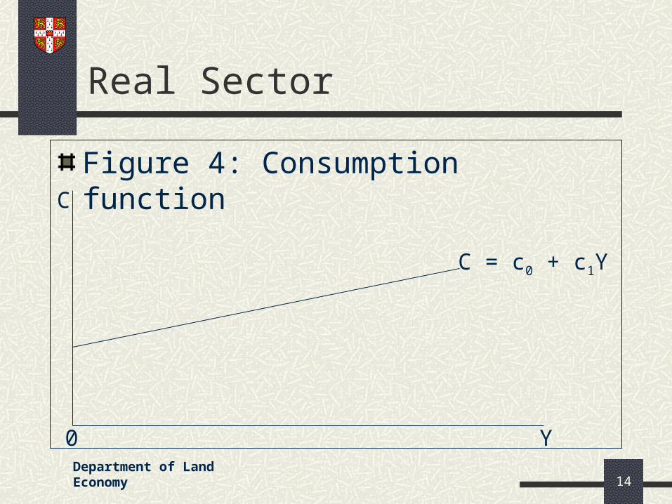
Absolute income hypothesis (Keynesian)

C = c0 + c1Y

where c0 is autonomous consumption, and c1 is the marginal propensity to consume (equal to

ΔC/ΔY, i.e. the slope of the consumption function).See Figure 4

c1 = 1 – s where s is the marginal propensity to save. No smoothing over time


Real Sector

Figure 4: Consumption functionC

Y

C = c0 + c1Y

0


Real Sector

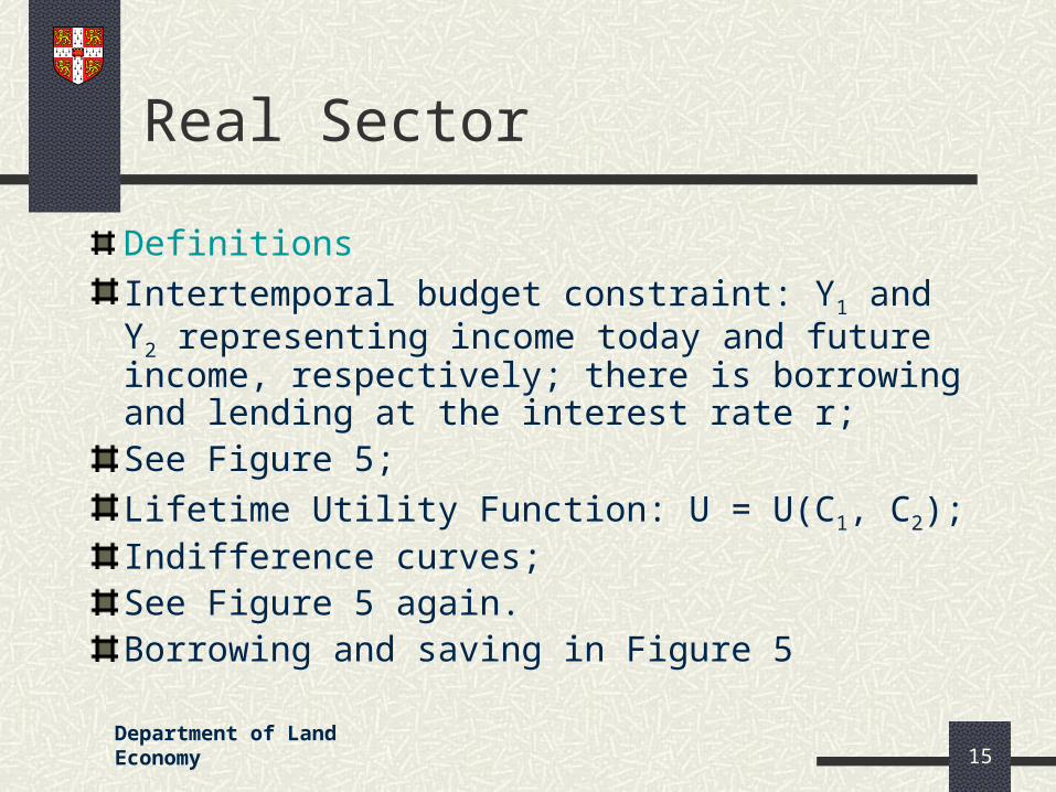
Definitions

Intertemporal budget constraint: Y1 and Y2 representing income today and future income, respectively; there is borrowing and lending at the interest rate r;See Figure 5;

Lifetime Utility Function: U = U(C1, C2);Indifference curves;See Figure 5 again.Borrowing and saving in Figure 5


Real Sector

Figure 5: Indifference curves

Y1(1+r)+Y2

Y1+Y2/(1+r)

Y’2

C2

Y2

Y’1 C1 Y1

Borrowing Saving

I1

I2


Real Sector

Consumption smoothing shown in Figure 5 forms the basis for permanent and life cycle theories of consumption. Permanent Income HypothesisY = Yp + YT

where Yp is permanent income, long-run or average income; and YT is transitory income. So that:

C = cpYp with 0 < cp <1. So, consumption is geared to permanent income, not current income. See Figure 6.


Real Sector

In figure 6, consider income Y1, which gives permanent consumption C1

P. If income is Y2, then we have consumption at C1

T, so that Y2’Y2 is then

transitory income. What permanent consumption would then be depends crucially whether the transitory component Y2

’Y2 is treated as permanent or not. If it is treated as permanent consumption is thereby C2

P.


Real Sector

Figure 6CLR

CSR

YY1

C1P

C2P

C1T

Y2’ Y2


Real Sector

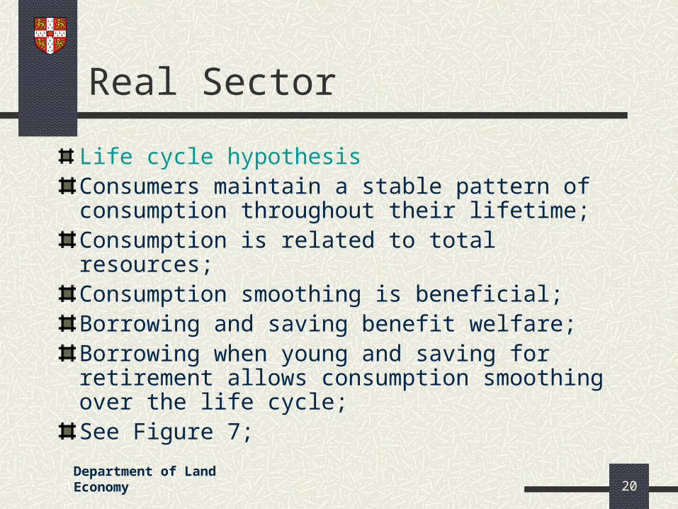
Life cycle hypothesisConsumers maintain a stable pattern of consumption throughout their lifetime;Consumption is related to total resources;Consumption smoothing is beneficial;Borrowing and saving benefit welfare;Borrowing when young and saving for retirement allows consumption smoothing over the life cycle;See Figure 7;


Real Sector

We may, thus, have:

Ct = wVt

where Vt is the present value of total resources;and

Vt = Wt-1 + Yt + [YtE/(1+r)n]

where the summation is over the remainder of the lifetime, Wt-1 is accumulated net wealth carried over from last period, Yt is current income and the third term is the present value of expected future income over the remainder of lifetime.


Real Sector

Figure 7

C

Time0

DissavingDissaving

Saving

Total Resources

C’


Real Sector

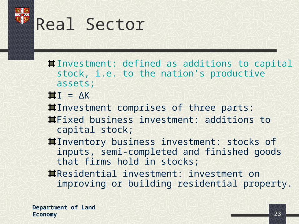
Investment: defined as additions to capital stock, i.e. to the nation’s productive assets;I = ΔK Investment comprises of three parts:Fixed business investment: additions to capital stock;Inventory business investment: stocks of inputs, semi-completed and finished goods that firms hold in stocks;Residential investment: investment on improving or building residential property.


Real Sector

In what follows we discuss investment without referring to its parts. We begin with the possibility that I=I(r).

V = R1/(1+r) + R2/(1+r)2 + ….. + Rn/(1+r)n

where V=present net value of future yields (R), and r is the rate of interest.


Real Sector

Compare V to the cost of undertaking investment (V’), so that if V>V’ new investment is undertaken; otherwise not.

As r changes, investment is affected. If r increases, V decreases and given V’ a lower volume of investment is undertaken. If r decreases then investment increases.


Real Sector

So that I = I(r): see Figure 8.If future yields change, the investment relationship shifts; a change in r means a movement along the I-relationship. Relationship can be shifted: expectations; technological change; stock of capital, etc.But if state of expectations is important, it can imply: I#I(r).


Real Sector

Figure 8

r

I0


Real Sector

An alternative way of approaching investment decisions is to ask what the discount rate (i) might be that equates V and V’, where V’ now is:

V’ = R1/(1+i) + R2/(1+i)2 + ….. + Rn/(1+i)n

and i is now called the marginal efficiency of capital; we then compare i with r, so that if i>r investment is undertaken; otherwise it is not. We may now explain how to derive Figure 8, where the I-relationship is depicted.


Real Sector

As r increases, the right-hand side of the equation decreases and the present value is now smaller than V’; also i tends towards r as investment decreases.As r decreases, the opposite happens; the right-hand side of the equation increases and the present value is now bigger than V’; also i tends towards r as investment increases.The two ways are alternatives and may not always give the same result since a change in r does not affect i systematically.


Real Sector

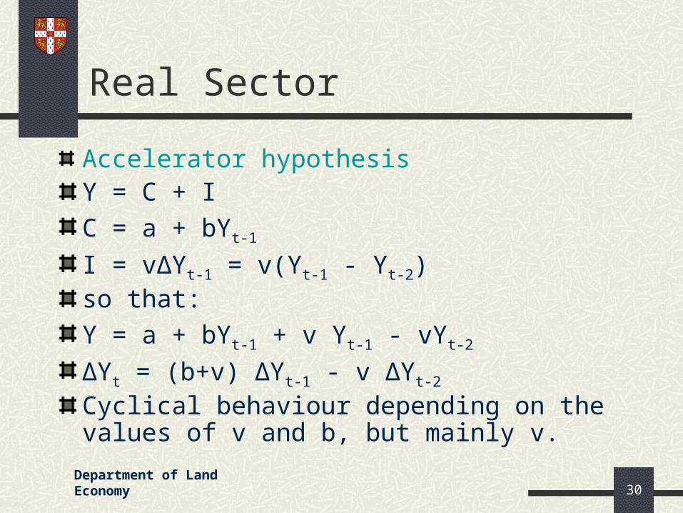
Accelerator hypothesisY = C + I

C = a + bYt-1

I = vΔYt-1 = v(Yt-1 - Yt-2)so that:

Y = a + bYt-1 + v Yt-1 - vYt-2

ΔYt = (b+v) ΔYt-1 - v ΔYt-2

Cyclical behaviour depending on the values of v and b, but mainly v.


Real Sector

0 < b < 1v = 0

0 < b < 1v = large

Cycles


Real Sector

Cycles

0 < b < 1v = relatively small

0 < b < 1v = relatively large


Real Sector

Tobin’s q

q = V0 / pkK0

where V0 is the market value of firm, which is

the expected discount future cash flows of

firm; and pkK0 is the replacement cost of installed

capital, where pk is the price of purchasing the firm’s

capital stock (K0).

Changes in q affects investment:


Real Sector

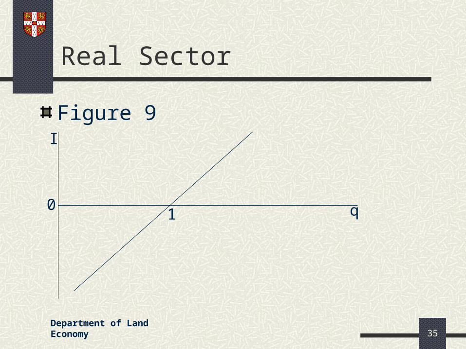
If q>1, then investment increases: installed capital produces higher market value for the firm. Thus investment increases; if q<1 the opposite happens. Thus investment decreases; if q=1 then nothing happens.

See Figure 9.


Real Sector

Figure 9

0 q

I

1


Real Sector

Residential investment

Tobin’s q theory fits nicely this type of

investment;

Clearly, qH = V0H /PH, where V0

H is the

discounted value of future rents; the cost of

building a house is given by the construction

price (PH).

It follows that: qH = R/rPH, from which:


Real Sector

If rPH is given, then as R increases, more residential investment is undertaken. What may determine rental value of housing is economic activity, i.e. income or unemployment.

Also for given R as the rate of interest increases and/or PH increases, then less investment is undertaken.


Real Sector

UK experience

R has been increasing; r has been low and PH has not been high; consequently q for investment should be very high. The evidence shows that housing construction is low! Why?High planning costs;Strategic action by planning developers, who may prefer gradual development for otherwise they might flood the market pushing R down!


Real Sector

Asymmetric information leading to credit rationing; this could come about in view of adverse selection and moral hazard;Adverse selection: lenders do not have full information about borrowers, who may not be able to repay in view of their high risk undertakings; this discourages ‘sensible’ borrowers;Moral hazard: borrowers act immorally; for example, depositors do not know banks, which may undertake high risks.


Real Sector

Government expenditure and taxes

Recall Y = [1/(1-c1)].(c0 - c1T + I + G)

(ΔY/ ΔG) = 1/(1- c1)

(ΔY/ ΔT) = [- c1/(1- c1)]

(ΔY/ ΔG) + (ΔY/ ΔT) = 1/(1- c1) + [- c1/(1-

c1)] = (1- c1)/(1- c1) = 1

i.e. balanced budget multiplier.


Real Sector

Crowding-outChanges in G, or T, has no impact on

Income; private expenditure is reduced at thesame time and by the same amount;

Crowding-In?Ricardian ModelRicardian consumers are rational, utility

maximisers, forward-looking and smoothconsumption over time;


Real Sector

Permanent income is more relevant thancurrent income;

Consequently, G and T policies wouldinfluence future spending and tax policies,which Ricardian consumers are able topredict; an increase in G means T increases infuture, so no impact on Y;

But real world a mixture of Ricardian and non-Ricardian consumers: fiscal policy still effective.


Monetary Sector

Money is anything that performs four functions: medium of exchange; unit of account; store of value; and standard of deferred payments;

Different definitions: M0, M1, M2, M3 etc;

Demand for Money: transactions motive, speculative motive and precautionary motive;

See Figure 10;

Demand for Money: MD = M(r, Y)


Monetary Sector

Figure 10

r

M0

Demand for Money (MD) = M(r, Y)


Monetary Sector

Supply of money (MS): Figure 11r

M0

SM


Monetary Sector

Money multiplier: it is:

(1) M = CP + D

(2) H = CP + R

(3) CP = cpD

(4) R = sD

So that:

(1)’ M = cpD + D = (1+ cp)D

(2)’ H = cpD + sD = (s+cp)D


Monetary Sector

So that:

M = [(1+cp)/(s+cp)].HM = mHWhere m is the money multiplierIf the elements on the right-hand side do not change endogenously, then M is exogenous; otherwise endogenous;Can it ever be exogenous in view of the central bank control of the rate of interest?


Monetary Sector

Equilibrium in the money market: Figure12:r

M0

re

MD=MS

SM


Monetary Sector

But, which interest rate?r is the nominal interest rate; R is the real rate of interest: what is the difference?Then value of £1 in the next period is: (1+r).1; but inflation in the next period is important: thus: (1+r) = (1+R).(1+πt+1), where πt+1 is the inflation rate in period t+1; this is approximated to:

r = R + πt+1 or:

R = r - πt+1

But r is normally assumed.


Monetary Sector

The LM relationship: Figure 13

M(r,Y0) M(r,Y1)

M(r,Y2)

r

M

r0

r1

r2

LM

r0

Y0 Y1

r1

0 YY2

r2

MS

0


Monetary Sector

The IS-LM model: Figure 14r

Y

LM

IS

re

Ye0


Foreign Sector

Open economy considerations: Figure 15 r

Y0

LM

IS

BP

re

Ye


Foreign Sector

Economic policy: fixed exchange rate: Figure 16r

Y0

re

Ye

IS

LM

BP

IS’

LM’

Ye’

re’ AB

C

B’


Foreign Sector

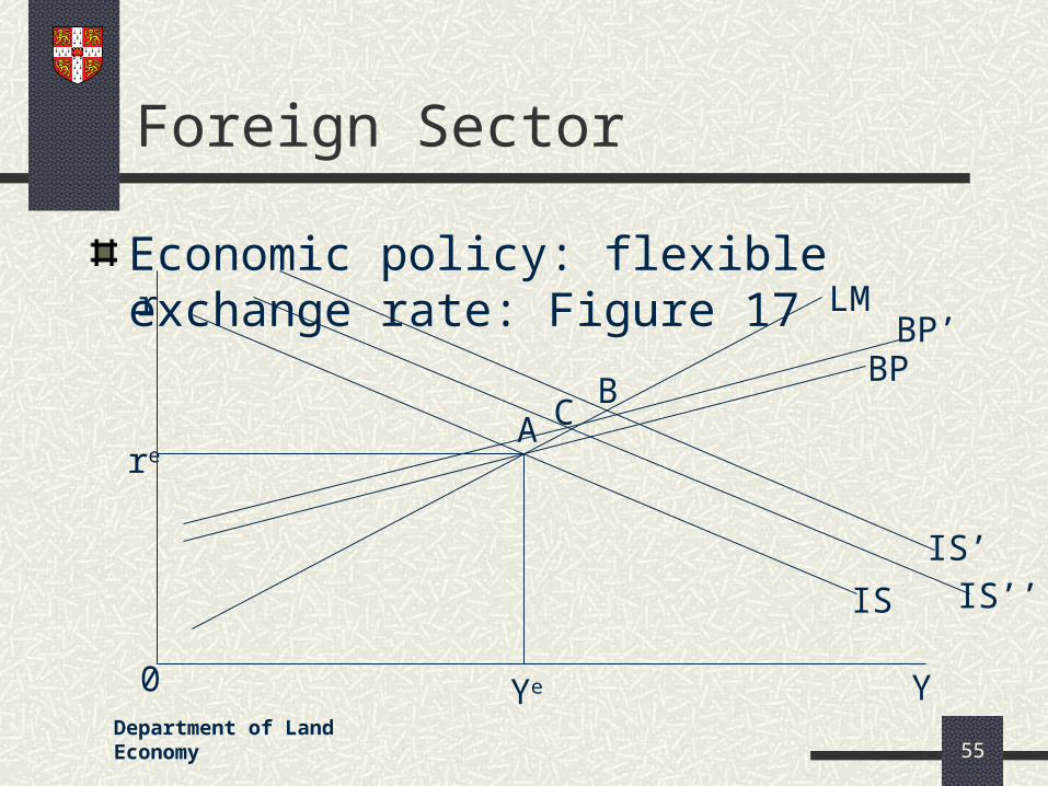
In Figure 16 (slide 53) we demonstrate the impact of fiscal and monetary policy in the case of the open economy with a fixed exchange rate;In Figures 17 (slide 55) and 18 (slide 56) we demonstrate the impact of fiscal and monetary policy in the case of the open economy respectively, assuming a flexible exchange rate;


Foreign Sector

Economic policy: flexible exchange rate: Figure 17r

Y

re

Ye0

IS

BP

LM

IS’

AB

BP’

C

IS’’


Foreign Sector

Economic policy: flexible exchange rate: Figure 18

IS

LMr

0 Y

re

Ye

BP

A

LM’

B

IS’

BP’

C


Inflation

Inflation: Figure 19r

Y

Y

0

0

Ye PC

LM

IS

P

Ye

re


Inflation

Inflation: Figure 20W/P

N

ND

NSW/P

NS-ND)/NS(W

U%

(W/P)e

Ne


Inflation

Inflation: Figure 21

SRPC1

LRPC

0

W

U%

SRPC2

U*U1

W1

W2

AB

C D


Inflation

InflationMV = PYMD = kPYMS = MS

MD = MS = MkPY = M, orP = (1/kY)M = (V/Y)Mi.e. the monetary theory of inflation (see Figure 22)


Inflation

Figure 22P

M0

P=(V/Y)M

P1

M1

P2

M2

M1 M2


Inflation

Figure 22 highlights the importance of controlling the money supply; also the importance of a stable demand for money;

If problems, i.e. monetary authorities not able to control the money supply or unstable demand for money, then controlling the money supply cannot control inflation;

Direct inflation targeting is the alternative.


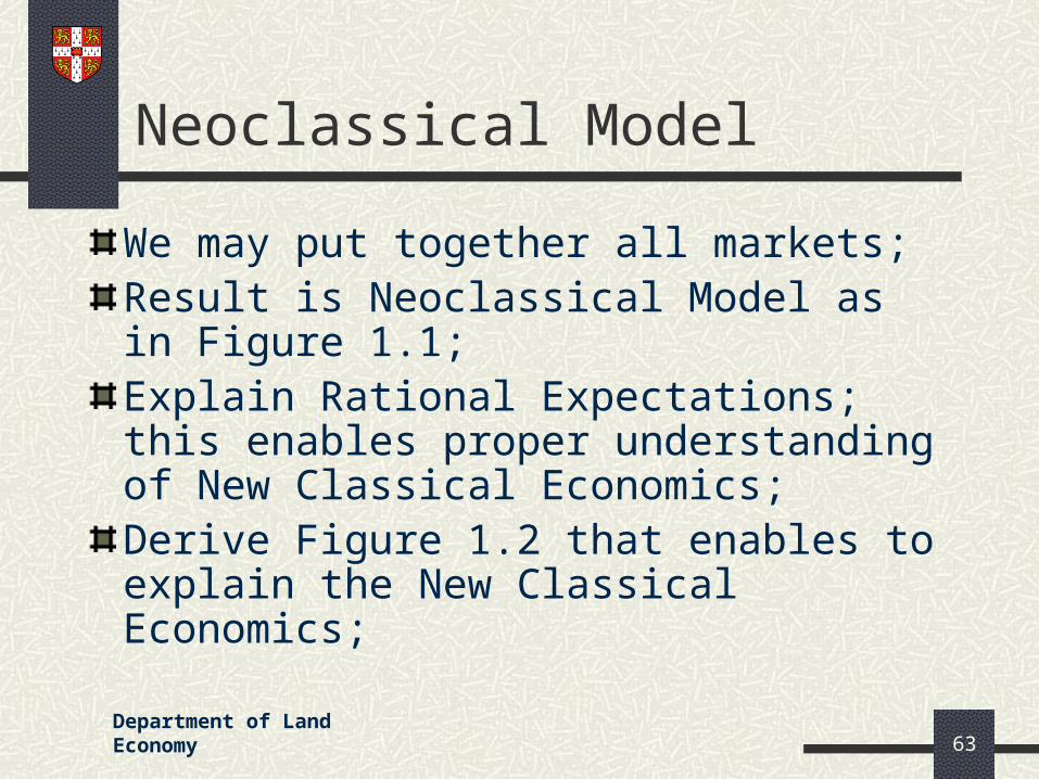
Neoclassical Model

We may put together all markets;Result is Neoclassical Model as in Figure 1.1;Explain Rational Expectations; this enables proper understanding of New Classical Economics;Derive Figure 1.2 that enables to explain the New Classical Economics;


Further Developments

Still further developments resulted in the New Keynesian Economics as in Figure 1.3;

Discuss policy attempts of the time at money supply control; but the point about money supply exogeneity should be made as a prelude to New Consensus Macroeconomics and Taylor Rule in particular;


New Consensus Macroeconomics

Eventually, and emanating from the New Keynesian Economics, the New Consensus Macroeconomics emerged;

Policy implications rather different from those of New Keynesian Macroeconomics: inflation targeting;

See subsequent slides in the rest of the lectures.

Documents

Department of Land Economy1 LECTURE 1 EMERGENCE OF NCM Philip Arestis University of Cambridge and University of the Basque Country