DEPARTMENT OF ECONOMICS

Milton Friedman, the Demand for Money and the ECB’s Monetary-Policy Strategy

Stephen Hall, University of Leicester, UK

P.A.V.B. Swamy, Retired from Federal Reserve Board George S. Tavlas, Bank of Greece, GR

Working Paper No. 12/05 April 2012

Milton Friedman, the Demand for Money and the ECB’s Monetary-Policy Strategy*

Stephen G. Hall Leicester University, Bank of Greece and Pretoria University

P.A.V.B. Swamy

Federal Reserve Board**

George S. Tavlas ***

Bank of Greece

ABSTRACT

The European Central Bank (ECB) assigns a greater weight to the role of money in its monetary-policy strategy than most, if not all, other major central banks. Nevertheless, reflecting the view that the demand for money became unstable in the early-2000s, some commentators in the press have reported that the ECB has “downgraded” the role of money-demand functions in its strategy. This paper explains the ECB’s monetary-policy strategy and shows the considerable influence of Milton Friedman’s contributions on the formulation of that strategy. The paper also provides new evidence on the stability of euro-area money-demand. Following a conjecture made by Friedman (1956), we assign a role to uncertainty in the money-demand function. We find that, although uncertainty is mean–reverting, it is none-the-less non-stationary, subject to wide swings, and has substantial effects on the demand for money.

Keywords: ECB’s monetary-policy strategy, Milton Friedman, money demand, JEL classification: C20; E41

* We are grateful to Eleni Argiri, Bill Gavin, Heather Gibson, Otmar Issing, Aggeliki Momtsia, Daphne Papadopoulou, Ifigeneia Skotida, Frank Smets, Mike Ulan, Hercules Vorides, and two referees for helpful comments. We are also grateful to Christina Tsochatzi and Sophia Xanthopoulou for technical support. We thank Thomas Vlassopoulos for providing us with the ECB’s data on wealth. The views expressed are those of the authors and should not be interpreted as those of their respective institutions. ** Retired. *** Corresponding author: George Tavlas, Director General, Bank of Greece, 21, E. Venizelos Ave., 102 50 Athens, Greece, Tel. +30210-320 2370 , Fax +30210-320 2432, email: gtavlas@bankofgreece.gr

1

1. Introduction

The primary objective of the European Central Bank’s (ECB’s) monetary-policy

strategy is to maintain price stability in the medium term.1

In a number of important respects, the ECB’s monetary-policy strategy reflects the

substantial influence of the research carried out by Milton Friedman during the 1950s and

1960s.

In pursuing that objective, the

ECB assigns more weight to the longer-term relationship between money growth and

inflation than most, if not all, other major central banks. This emphasis reflects, in part, the

ECB’s views that (1) “inflation is ultimately a monetary phenomenon”, and (2) “price

stability enhances the potential for economic growth” (ECB, 2011, pp. 55-56). Effectively,

the emphasis reflects the notion that longer-term growth is determined by real factors --

including an economy’s resources, the growth of its population, and the technical skills of its

labor force -- and that the most that monetary policy can do to help the economy reach its

growth potential is to deliver a stable price level (ECB, 2011, p. 56).

2

In this paper, we explain the key linkages between Friedman’s work, including the

relevance of a stable money-demand function, and the strategy adopted by the ECB. We also

provide new evidence on the stability of euro-area money demand based on a framework that

captures the effect of uncertainty on the demand for money, an idea first proposed by

Friedman (1956).

One such respect concerns the stability of the demand for money, which helps

underpin the idea that there exists a reliable, longer-term relationship between the growth in

the money supply and inflation. Friedman (1959) found that demand for money in the United

States was stable, a finding that was corroborated for the euro area in early work by the staff

at the ECB (Calza, Gerdesmeier, Levy, 2001). However, beginning around 2003, most euro-

area money-demand functions began exhibiting instability, leading some commentators in

the press to infer that the role of money had been “downgraded” in the ECB’s monetary-

policy strategy (see Section 3).

The remainder of this paper is structured as follows. To set the stage, Section 2 provides

an overview of Friedman’s earlier research findings, which, as we show, underpinned his

famous policy proposal for a constant money-supply growth rate, first published in 1958.

Section 3 describes the monetary-policy strategy of the ECB, including the role of the 1 The ECB’s definition of price stability is given in Section 3. 2 Elements of Friedman’s thinking can be found in the monetary-policy strategies of other central banks, including those that follow inflation targeting. For an acknowledgement of Friedman’s views in influencing the Federal Reserve’s policy, see Bernanke (2002).

2

demand for money in that strategy; that section also describes the influence of Friedman’s

work on the ECB’s monetary-policy strategy. We show that, although the finding in the mid-

2000s by ECB economists that the demand for money in the euro area was no longer stable

led to what the press reported as a “downgrading” of the role of money in the ECB’s

strategy, the role of monetary analysis in the ECB’s strategy remains pivotal in assessing the

outlook for future price developments. Section 4 turns to our analysis of euro-area money-

demand. That section provides the basic theoretical framework we use to estimate money-

demand. Unlike previous empirical studies of money-demand, we include a measure of

economic sentiment to capture the effect of uncertainty on money-demand. As pointed-out

by Friedman (1956), and as reflected in the capital asset pricing model, at times of declining

confidence (or increasing uncertainty), any asset should yield an increased rate of return in

order to compensate for the increased risk. If the rate of return does not rise to mirror the

increase in uncertainty, there will be a flight into liquid assets, such as money. This

confidence effect can be extremely important during times of crises. The recent crisis in the

euro area provides an apt setting to test that hypothesis. Section 5 describes the two

empirical methodologies we use to estimate euro-area money demand: (1) the workhorse

vector-error-correction (VEC) approach, and (2) a generalized cointegration approach, which

is estimated on the basis of a time-varying-coefficient (TVC) technique. Section 6 presents

the empirical findings. To anticipate briefly, both empirical methodologies suggest that,

taking account of uncertainty, the long-run demand for money in the euro area has been

stable. We find that, although uncertainty is mean–reverting, it is none-the-less non-

stationary, subject to wide swings and has substantial effects on the demand for money.

Section 7 concludes with the implications for the ECB’s monetary-policy strategy.

2. How the Constant Money-Supply Rule was Formed

Friedman joined the University of Chicago faculty in 1946 and remained at that

institution until his retirement from teaching (and his move to the Hoover Institution) in

1977. He began collaboration with Anna Schwartz in 1948 on U.S. monetary history; around

the same time that he began conducting a Workshop in Money and Banking at the University

of Chicago.3

3 The collaboration with Schwartz resulted in this classic, A Monetary History of the United States, 1867-1960, published in 1963. In his initial correspondence with Schwartz, Friedman estimated that their project would be completed in three years. See Tavlas (2012), upon which the discussion in this section draws.

He first proposed the constant money-growth rule in a 1958 paper, “The Supply

of Money and Changes in Prices and Output”, submitted to the Congressional Joint

3

Economic Committee.4 Friedman (1958, p. 174) stated that his aim was to summarize “the

preliminary results” of his work with Schwartz and the series of studies conducted in the

Chicago Workshop in Money and Banking, conducted under Friedman’s direction. A main

implication of those results is the need to distinguish between long-run, or secular, empirical

relationships and short-run, or cyclical, relationships; the former tend to show considerable

stability whereas the latter are subject to large uncertainty. The money growth-rate rule was

formulated on the basis of long-run relationships. The following discussion draws on three

studies: (1) the 1958 study presented to the Joint Economic Committee; (2) a 1959 paper,

“The Demand for Money: Some Theoretical and Empirical Results”, published in the

Journal of Political Economy, and (3) a 1960 book, A Program for Monetary Stability,

which was based on a series of lectures Friedman gave at Fordham University in 1959. The

discussion focuses on those empirical findings that underpinned the money growth-rule.5

2.1 The long-run

Money and prices. The historical evidence suggests that there is a strong empirical

regularity between changes in the stock of money per unit of output and changes in prices in

the same direction. Friedman (1958, p. 173) noted that this regularity “tells nothing about

direction of influence”. However, the variety of monetary arrangements - - for example, the

gold standard, flexible exchange rates, regimes with and without a central bank, changes in

the structure of the Federal Reserve System and commercial banking, shifts in leadership of

the Fed - - over which this regularity has been observed “supports strongly… [the view] that

substantial changes in the stock of money are both a necessary and sufficient condition for

substantial changes in the general level of prices” (1958, p. 173).

Definition of money. How should the money supply be defined? Friedman argued that

“there is a continuum of assets possessing in various degrees the qualities we attribute to the

ideal construct of ‘money’ and hence there is no unique way to draw a line separating

‘money’ from ‘near-moneys’” (1960, p. 90). The “most useful concept” is that

corresponding to currency held by the public plus adjusted demand deposits plus time

4 The paper was published as part of the collected essays in Friedman (1969). 5 It should be kept in mind that the Friedman and Schwartz evidence to which Friedman referred in these studies was preliminary. Moreover, during the 1960s Friedman’s views on some of the issues discussed below, including the Great Depression, would undergo refinement. The data periods to which Friedman referred in these studies alternated among either 1867-1954, 1867-1957, and 1870-1954.

4

deposits in commercial banks6

Output and prices. Historical evidence indicates that there is no clear-cut relation

between price changes and output changes. The “only conclusion” that can be drawn from

this evidence is that “either rising prices or falling prices are consistent with rapid economic

growth, provided that the price changes are fairly steady, moderate in size, and reasonably

predictable” (1959, p. 184). The underpinnings to economic growth are to be found in such

factors as “available resources, the industrial organization of a society, the growth of

knowledge and technical skills, the growth of population, the accumulation of capital and so

on” (1959, p. 182). On average, over a period of 90 years (from 1867-1957), the average

annual growth in output has been “something over three percent” (1960, p. 91).

“because it seems more closely related empirically to income

and other economic magnitudes than other concepts” (1960, pp. 90-91, italics supplied).

Income velocity. Friedman (1959) reported empirical findings of his work with

Schwartz on secular changes in the real money stock per capita and secular changes in real

income per capita over the period 1870 to 1954 for twenty reference cycles measured from

trough to trough. The observations consisted of average values of the variables concerned

over the complete cycle. The findings showed that “secular changes in the real stock of

money per capita are highly correlated with secular changes in real income per capita”

(1959, p.113). The correlation coefficient between the logarithm of the real stock of money

per capita and the logarithm of real income per capita was found to be 0.99 and the

computed elasticity was 1.80 (1959, p.113). Hence, a one per cent increase in income per

capita was, on average, associated with a 0.80 decrease in income velocity. Friedman noted

that the high correlation could be a reflection of trends in the data so that the results might

“not justify much confidence that the statistical regression is a valid estimate of a demand

relation rather that the result of an accidental difference in trends” (1959, p.113). He noted,

however, that “additional evidence from other sources leads us to believe that it can be so

regarded” (1959, p.113).

In the same paper (1959), Friedman’s (log-linear) estimation of the demand for money

corroborated the above findings. The specification of the money-demand function consisted

of the following elements: (1) the dependent variable was nominal cash balances (i.e., M2)

per capita; (2) the explanatory variables were measures of permanent income, permanent

prices and population; and, (3) the estimation period was 1870 to 1954. Using average values

6 Subsequently, this measure corresponded to what became known as M2.

5

of the variables over the cycle (measured from trough to trough),7 Friedman (1959, pp. 126-

27) estimated an income elasticity of nominal cash balances of 1.810 which implied a

velocity elasticity of -0.810. He then used these parameters to compute annual estimates of

velocity, which he compared with the actual figures. He found that the estimates accounted

for “the bulk of the fluctuations of measured velocity” (1959, p. 130). “These results”, he

argued, “give strong support to the view that cyclical movements in velocity largely reflect

movements along a stable demand curve for money” (1959, p. 130).8

2.2 The short run

The foregoing secular empirical relationships, Friedman found, do not hold tightly

within the business cycle. In his paper for the joint Economic Committee, Friedman (1958,

p. 179) reported that his research with Schwartz revealed that, although there is a close link

between monetary changes and price changes within the business cycle, “the direction of

influence between the money stock and income and prices is less clear-cut and more

complex for the business cycle than for the longer movements”. This circumstance, he

argued, reflected three factors.

First, “the character of our monetary and banking system means that an expansion of

income contributes to expansion in the money stock, partly through inducing banks to trim

more closely their cash reserve position, partly through a tendency for currency in public

hands to decline relative to deposits” (1958, p. 179). Thus, Friedman argued that, during the

business cycle, changes in the money supply are “a consequence as well as an independent

cause of changes in income and prices” (1958, p. 179). Moreover, once a cyclical expansion

or contraction is started the process is self-generating: “once they [changes in money,

income and prices] occur, they will in their turn produce further effects on income and

prices” (1958, p. 179).

Second, consideration of the timing of changes in the money supply, income and

prices complicates the relationship among those variables, making it more difficult to infer

an independent influence of monetary change within the cycle than for secular movements.

Within the cycle, the relationship among these variables is subject to lags. His work with

7 As Lothian (2008, p. 1089) pointed out: “By using reference-cycle averages as his basic units of observation, Friedman was able to focus on positions of long-run equilibrium. He, therefore, was able to get around to the problems of monetary endogeneity and the partially related econometric problems inherent in modelling short-run monetary adjustment.” 8 See, also, Friedman (1958, p. 175), which cited evidence on velocity behavior in papers by Cagan (1956) and Selden (1956), both of which were written for the Chicago Workshop in Money and Banking.

6

Schwartz provided quantitative estimates of the lags; the lags were found to be long - - on

average, the rate of change in the money supply was found to have reached its peak nearly

16 months before the peak in economic activity and to have reached its trough over 12

months before the trough in economic activity - - and the lag lengths were found to have

varied considerably from cycle to cycle (1958, p. 180; 1960, p. 88).

Third, and related to the previous factor, within the cycle, real shocks to velocity have

been a source of economic fluctuations (1958, p. 89). Discretionary monetary policy in

reaction to those shocks serves to amplify the effects of those real disturbances on the

economy.9

2.3 The policy rule

In the absence of the reaction of monetary policy, the shocks would merely

constitute “the myriad of factors making for minor fluctuations in economic activity” (1959,

p. 144).

The above evidence underpinned Friedman’s proposal that the money supply - -

defined as currency held by the public plus demand and time deposits in commercial banks

(M2) - - should increase by between 3 to 5 per cent per year (1958, p. 184). The secular

empirical relationships informed both the particular concept of money used and the

numerical margins (i.e., 3 to 5 per cent) of the growth range. Specifically, he chose M2

because of its close empirical relationship to “income and other economic magnitudes”

(1960, p. 91).10

Why conduct policy in terms of a rule instead of using discretion? In his 1960 A

Program for Monetary Stability, Friedman (1960, p.86) argued that a rule would be easy to

understand and would eliminate “the danger of instability and uncertainty of policy”.

Friedman (1960, p. 85) also argued that discretion absolves the policymakers of any criteria

from which to judge their performance and leaves them vulnerable to political pressures

(1960, p. 85). Finally, relying on the evidence of his work with Schwartz on short-term

During the period 1867-1957 output growth, Friedman noted, had averaged

about 3 per cent a year, while velocity had exhibited a secular decrease of about 1 per cent a

year (1958, pp. 184-85; 1960, pp. 90-91). Thus, “to judge from this evidence, a rate of

increase [of M2] of 3 to 5 per cent per year might be expected to correspond with a roughly

stable price level for this particular concept of money” (1960, p. 91).

9 In a 1973 paper, Friedman argued that “if we knew about autonomous changes in the real demand for money, it would be right to adjust the money supply to them. However, we don’t know about them” (Friedman 1973; quoted from Nelson, 2008, p. 101) 10 Friedman (1960, p. 91) stated that “the evidence for this concept is certainly far from conclusive.” In the early-1980s he switched to M1. Nelson (2007) provides a discussion of the reasons for the switch.

7

relationships, Friedman (1960, p. 85) argued that, in the past, discretion had led to “continual

and unpredictable shifts in policy and in the content of policy as the persons and attitudes

dominating the authorities had changed”. A money growth rule, he believed, would have

avoided the “excessive” mistakes of the past, including the collapse of money from 1929 to

1933, the discount-rate increases of 1931, and the resulting depression (1960, p. 93). It

would not rule out mild cyclical fluctuations, but it “would almost certainly rule out…rapid

and sizeable fluctuations” (1960, p. 92). Friedman (1960, p. 90) agued that the

implementation of his money supply proposal has a further advantage; “it would largely

separate the monetary problem from the fiscal [problem]”. As discussed in the following

section, the Friedman’s empirical findings with regard to both the long-run and the short-run

helped shape the monetary-strategy adopted by the ECB.

2.4 The Phillips curve and expectations

In addition to the above contributions made during the 1950s, another contribution by

Friedman that would later have an impact on the ECB’s monetary-policy strategy was

Friedman’s rebuttal of the traditional Phillips-curve notion that there exists a permanent

trade-off between the unemployment rate and the inflation rate. Along with Phelps (1968),

Friedman (1968) demonstrated that the steady-state unemployment rate is not related to the

steady-state inflation rate when the Phillips relationship is augmented by a variable

representing the expected inflation rate -- that is, labor negotiates on the basis of real, and not

nominal, wages. Consequently, in the long run there can only be varying levels of the

inflation rate – which, in turn, depend on the steady-state change in the money supply -- with

the same “natural” level of the unemployment rate. This insight was a formalization of

Friedman’s earlier (1950s) research showing that, in the long-run, the monetary authorities

can only control nominal values.

3. The ECB’s Monetary Policy Strategy

As noted in the introduction, the primary objective of the ECB’s monetary policy is to

achieve price stability in the medium term.11 The Governing Council12

11 The meaning of medium term has not been precisely defined by the ECB.

of the ECB defines

12 The ECB is governed by two main decision-making bodies - - the Governing Council and the Executive Board. The Governing Council is the main decision making body. It combines the six-member Executive Board (which includes the President and Vice President of the ECB) and the 17 governors of the National Central Banks of the Member States that have adopted the euro. The Governing Council usually meets twice a month in Frankfurt, Germany. At its first meeting each month, the Governing Council assesses economic and monetary developments and takes its monthly monetary policy decision. At its second meeting, the Council discusses issues mainly related to other tasks and responsibilities of the ECB.

8

price stability as a year-on-year increase in the Harmonized Index of Consumer Prices

(HICP) for the euro area of “below, but close to, 2 per cent in the medium term” (ECB,

2011, p. 64).13

3.1 The influence of Friedman

The ECB sees several advantages in this particular formulation of its policy

objective (Issing and Tristani, 2005, pp. 62-64; Carboni, Hofmann and Zampoli, 2010; ECB,

2011, pp. 64-67). First, it is easy to understand, thereby contributing to the transparency of

monetary policy. Second, it provides a yardstick with which to gauge the ECB’s

performance, thus providing accountability. Third, it provides an anchor for the formation of

price expectations, under the assumption that expectations of inflation are a key determinant

of actual inflation. Fourth, it provides a “safety margin” between the price-stability objective

(below, but close to, 2 per cent) and zero inflation. Fifth, it helps deal with the issue of the

possible presence of upward measurement-error bias in the HICP, whereby, the measured

inflation rate may over-estimate the “true” inflation rate because the former does not

adequately reflect such factors as improvements in the quality of products. Sixth, because the

definition does not specify a precise numerical objective, it provides some allowance for

inflation differentials within a monetary union comprised of heterogeneous countries.

Many of the foregoing advantages attributed by the ECB to the formulation of its

policy objective have been influenced, explicitly or implicitly, by Friedman’s work.14

• As noted above, the main objective of Friedman’s money-growth rule was to

eliminate policy uncertainty. In explaining the rationale for the ECB’s monetary

policy strategy, Issing, Gaspar, Angeloni, and Tristani (2001, p. 99) stated: “the

structure of any monetary policy strategy must reflect the extent and the nature of

the uncertainties faced by the central bank. Different prevailing sources of

uncertainty will normally require different strategies, i.e. differences in the way

information is processed in order to attain policy decisions. The ECB strategy, in

particular, was tailored having specifically in mind the uncertainties existing in the

conduct of the single monetary policy….”

In this

regard, consider the following influences.

13 The HICP is a weighted average of price indices of the member states of the euro area. Its coverage includes goods and services consumed. The index measures the change in expenditure necessary to maintain unchanged, with respect to a base period, the consumption pattern of households and the composition of the consumer population. See Issing, Gaspar, Angeloni, and Tristani (2001, pp. 51-53). 14 It is important to note that the ECB’s monetary-policy strategy reflects a broad range of contributions other than those of Friedman. For a good discussion, see Issing, Gaspar, Angeloni, and Tristani (2001, pp. 32-46).

9

• Friedman expressed the view that an advantage of his constant money-growth

proposal was that it would be easy to understand, while holding policymakers

accountable for their actions (Friedman, 1960, pp. 85-90). The ECB’s medium-

term price-stability objective is based, in part, on the criteria of transparency and

accountability.

• The ECB’s emphasis on the price level -- a nominal magnitude -- “echoes

recommendations put forward by Milton Friedman” [that] the monetary authority

can control nominal, but not real, variables (Issing and Tristani, 2005, p. 10)

• The medium-term orientation is an explicit acknowledgement “that Milton

Friedman’s assertion about the long and variable lags of the [monetary]

transmission mechanism remains valid” (Issing and Tristani, 2005, p. 29). It is also

an acknowledgement of “the possibility emphasized by Friedman… that counter-

cyclical policy may actually increase instability in economic activity” (Issing,

Gaspar and Vestin, 2005, p. 120).

• As mentioned above, Friedman wrote that it was important to maintain a clear

separation of monetary policy from fiscal policy. Article 123 of the Treaty of the

Functioning of the European Union (the Treaty), which is the legal basis of the

ECB’s setting of monetary policy, prohibits the monetary financing of fiscal

actions, thereby drawing a clear line of separation between monetary policy and

fiscal policy (ECB, 2011, p. 15).

• An objective of Friedman’s (1960, p. 93) money-growth rule was to provide

independence for the monetary authorities. Article 130 of the Treaty lays down an

“institutional framework for the [ECB’s] monetary policy [under which the]

central bank … is independent from political influence” (ECB, 2011, p.14).15

• The idea that expectations of inflation are a key determinant of present inflation is

directly related to Friedman’s (1968) augmentation of the Phillips curve, under

which the actual inflation rate was shown to be dependent on a variable

representing the expected inflation rate.

15 The ECB’s monetary-policy strategy was, to a substantial extent, based on the earlier strategy of Germany’s Bundesbank. Issing and Tristani (2005, p. 50) discussed the influence of Friedman on the Bundesbank’s strategy.

10

3.2 The two-pillar approach

In pursuing its objective of price stability, the ECB’s Governing Council regularly

assesses risks to price stability on the basis of two organizing perspectives - - known as the

“two pillars”. The first pillar is the “economic analysis”, which assesses the short-term to

medium-term influences on price developments, with a focus on the real-activity and cost

factors (e.g., wages, oil prices) driving prices over these horizons. The focus of this pillar is

on the interplay of supply and demand in the goods, services and factor markets. The second

pillar is the “monetary analysis”. It exploits the long-run link between money and prices, and

serves as a “cross-check, from a medium-term to long-term perspective, on the short-term to

medium-term assessments derived from the economic analysis” (ECB, 2011, p. 69). This

longer-run link between money and inflation was expressed by Issing (2008, p. 105) as

follows: “The close relationship between the money supply and prices has been proven in

countless studies all over the globe and all through history… Milton Friedman expressed this

insight in a nutshell: inflation is always and everywhere a monetary phenomenon. In his

analysis there is no case where a significant change in the quantity of money per unit of

output has not been associated with a significant increase in the price level”.

The two pillars comprise complementary perspectives of the determinants of inflation

(Carboni, Hofmann, and Zampoli, 2010, p. 57). As mentioned, the economic-analysis pillar

seeks to identify risks to price stability at short to medium-term horizons. The monetary-

analysis pillar seeks to identify risks to price stability at medium to long-run horizons. As is

the case with the economic analysis, the monetary analysis is broad-based in that it takes into

account information provided by a wide range of monetary indicators, including interest

rates, asset prices, and various definitions of the money supply and their components and

counterparts - - for example, credit and several measures of excess liquidity (Carboni,

Hofmann, and Zampoli, 2010, p. 57). As the ECB’s then-President Trichet (2006) put it:

“the European experience - - both before and after the euro - - suggests that assigning an

important role to money in monetary policy deliberations and communications in practice,

helps to serve precisely those principles that modern monetary policy literature holds dear ...

[when] the economic analysis is complex and its conclusions uncertain, cross-checks with

the monetary analysis have proved extremely useful.”16

At the inception of the ECB, that institution announced a “reference value” for

monetary growth. An aim of the reference value was to help account for the long-run

16 For a detailed discussion of the monetary-analysis pillar, see Drudi, Moutot and Vlassopoulos (2010).

11

relationship between money and prices. The construction of this reference value followed

closely Friedman’s construction of a money-growth rule. From the various definitions of

money, that aggregate was chosen that has demonstrated the “best fit” with prices (Issing,

2008, p. 108). On the basis of the “best-fit” criterion, a broad measure of money, M3, was

selected: M3 consists of currency in circulation plus overnight deposits (M1) plus deposits

with agreed maturity of up to two years (M2), plus repurchase agreements plus money

market fund shares plus debt securities up to two years17

Several aspects of the M3 reference value are important to mention. First, the reference

value is a medium-term norm rather than a monetary target (ECB, 1999; Issing, Gaspar,

Angeloni, and Tristani, 2001); deviations of M3 growth from the reference value do not

entail a commitment to correct the deviations (Issing, 2008, p. 108). Second, as noted, in

addition to the reference value the monetary pillar is comprised of a broad array of monetary

and financial-market data, including various credit aggregates and interest rates. Third, as

discussed above, the M3 reference value is, in part, predicated on a stable M3 demand

function. In this connection, for many years following the inception of the euro on January 1,

1999, euro-area consumer price inflation was close to 2 per cent, with little volatility, while

M3 growth was almost always above its reference value, peaking at 12½ per cent (year-on-

year) in late 2007 (Figure 1), implying that the relationship upon which the 4½ per cent

reference value for M3 growth was based was no longer valid. Correspondingly, the

consensus view that emerged from virtually all euro-area empirical money-demand studies

beginning from the early 2000s was that of an unstable M3 demand function (e.g., Beyer,

Fischer, and von Landesberger, 2007; Fischer, Lenza, Pill, and Reichlin, 2007; Fischer and

Pill, 2010).

. The trend growth of real GDP was

estimated by the ECB to be between 2 to 2.5 per cent per year and the trend (decline) in

velocity was estimated to be 0.5 to 1.0 per cent per year. Based on these estimates, and the

definition of price stability (annual inflation close to, but below, 2 per cent), the ECB set a

reference value for M3 growth of 4 ½ per cent per year.

The impact of the finding of an unstable money-demand function for the ECB’s

monetary analysis was highlighted at an ECB conference on “The Role of Money: Money

and Monetary Policy in the Twenty-First Century”, in Frankfurt in November 2006. At that

conference, ECB staff acknowledged that M3 demand functions had broken down, 17 The sample period used by the ECB to estimate the “best-fit” criterion typically begins in 1980. Since euro-wide data were not available prior to the start of the euro area on January 1, 1999, data extending backward to 1980 were constructed “synthetically”.

12

prompting some press commentators to infer that the role of money-demand had been

downgraded. Thus, the German newspaper, Handelsblatt (November 10, 2006), reported on

the conference proceedings as follows:

The ECB managed to bring together most of the leading academic experts in monetary policy to present papers on and discuss the role of money in monetary policy….The ECB’s [then] Director General for Research, Lucrezia Reichlin, presented a paper co-authored with three ECB colleagues, in which she presented some hitherto unpublished information about the development of monetary analysis within the ECB. The paper … contained a comparison of the accuracy, bias and volatility of inflation forecasts derived from monetary and other indicators….. Reichlin stressed that the ECB had found money demand not to be stable and had consequently downgraded the role of money demand functions in its analysis.

The Financial Times (November 10, 2006) reported on the same conference as follows:

The ECB’s “monetary pillar,” largely inherited from Germany’s Bundesbank, is controversial among economists because of confusion about the implications of money supply for inflation. At the ECB-hosted conference, prominent officials from the Frankfurt institution made clear that they saw significant scope for refinements….ECB research presented at the conference was open about the shortcomings of the bank’s monetary analysis in its eight-year history (Atkins, 2006).18

Reflecting the above developments, with regard to money-demand during the past ten

years or so the ECB has changed the role of the M3 reference value.

• From 1999 until 2003, the ECB conducted annual reviews of the reference value.

Those reviews signaled that the ECB attached importance to the concept of a

reference value.

• In order to highlight the medium-term context of the ECB’s monetary-policy

strategy, the annual reviews were discontinued in May 2003. This discontinuation

implied that the M3 reference value was assigned a smaller role than previously

under the monetary-analysis pillar.

• Subsequently, the role of the reference value was subsequently diminished further.

As a result, the ECB presently uses deviations of M3 from the reference value as a

“trigger” for “increased efforts to identify and assess the nature and persistence of

18 The paper upon which Reichlin’s presentation was based was a co-authored paper; the co-authors were Fischer, Lenza, Pill, and Reichlin (2006). The paper itself, while acknowledging the breakdown of euro-area money-demand relationships, stressed the importance of monetary factors and the need to develop new tools to assess the impact of monetary factors on the economy.

13

the forces responsible” (ECB, 2011, p. 80). Effectively, the reference value no

longer has any direct impact on ECB decision-making.

In light of the importance attached to the finding of an unstable money-demand

function in the developments described above, a question that arises is: How robust is that

finding? To address this question, beginning in 2007, the ECB set-up a research program

that created an organizational framework for the “enhancement of [the ECB’s] monetary

analysis” (Papademos and Stark, 2010, p. 8). Essentially, the enhancement involves (1) a

deepening of monetary-analysis pillar through the development of new analytical tools that

explore the relationship between monetary trends and underlying inflation dynamics, and (2)

a broadening of the monetary-analysis pillar to assess the interaction of monetary variables

with a wider set of economic and financial factors (Papademos and Stark, 2010, p. 9). In

light of the role played by money-demand equations to the ECB’s monetary-analysis pillar,19

one of the major objectives of the enhancement program has been to provide a means for

“improving models of euro area money demand” (Papademos and Stark, 2010, p. 8).20

4. Theoretical Underpinning

We

provide our contribution to this issue in what follows.

We consider euro-area money demand in the spirit of the framework proposed by

Friedman (1956) and Brainard and Tobin (1968). Those authors postulated that money, like

any asset, yields a flow of services to the agents who hold it. As under the usual theory of

consumer choice, Friedman (1956, p. 4) argued that the demand for money depends on three

major sets of factors: (1) total wealth - - the analogue of the budget constraint, and

comprised of both non-human capital and human capital, (2) the price of, and return to,

wealth21

19 Fischer and Pill (2010, p. 131) wrote: “Money-demand models are the workhorse of [the ECB’s] monetary analysis, playing an unglamorous but crucial role in any comprehensive framework for the assessment of monetary conditions.”

, and (3) the tastes and preferences of the wealth-owning units. He also argued that

the proportion of wealth held as money is likely to be affected by the level of uncertainty.

Friedman (1956, pp. 8-9) wrote: “it seems reasonable that, other things the same, individuals

want to hold a larger fraction of their wealth in the form of money when they are subject to

20 Of the two press reports cited above on the November 2006 ECB conference - - those of Handelsblatt and the Financial Times - - the latter was more accurate about the implications of the conference for the ECB’s monetary-analysis pillar. Although money-demand models had been found to have broken down, the ECB responded by attempting to improve those models. 21 Friedman (1956) specified a money-demand function in which the real quantity of money demand is a function of a vector of returns on alternatives to holding money-bonds, equities, physical goods, and human capital.

14

unusual uncertainty than otherwise. This is one of the major factors explaining a frequent

tendency for money holdings to rise relative to increases in income during wartime.”

Brainard and Tobin (1968) and Tobin (1969) also stressed the role of wealth in the

money demand function. Those authors argued that, in contrast to conceptual approaches

that treat income and wealth interchangeably as determinants of money demand, an increase

in wealth results in increases in the demand for all assets, whereas an increase in income

increases the demand for money at the expense of other assets. Therefore, both income and

wealth belong in the money-demand function. We follow the Brainard-Tobin approach in

this paper.22

Specifically, we use a portfolio-balance model to estimate the demand for money.

Assuming that the asset choices of investors involve money and equities, the demand for real

money balances can be written as follows (where the symbols above the explanatory

variables indicate the expected direction of influence on real money balances):

),,,,( lesiprprwyfpm eeem −+++−−=− (1)

where m is the log of nominal M3, p is the log of the price level, y is the log of real

income, w is the log of the real value of wealth, mr is the own rate of return on money, ep

is the expected inflation rate, er is the opportunity cost of holding money balances, and,

reflecting Friedman’s (1956) emphasis on the role of uncertainty on money-demand, lesi

represents investors’ confidence (which we define below). In equation (1), real rates of

return are approximated by nominal rates minus the expected inflation rate.

We also assume rate-of-return homogeneity of degree zero, implying that, if all rates of

return change by x per cent, real quantities of assets in investors’ portfolios relative to real

income and real wealth will not change. Thus, only rates-of-return differentials affect money

demand. Rate-of-return homogeneity implies that we can use interest differentials, selecting

one of the assets as numeraire; we use m as a numeraire. Therefore, the money-demand

function can be re-written as:

),,,( lesirrwyfpm me−++−=− (2)

When f is semi-log linear, the money-demand function becomes: 22 Friedman (1956, pp. 4-9; 1959) considered permanent income to be the relevant measure of wealth in the demand-for-money function. In addition to permanent income, he argued that a variable capturing the ratio of wealth-to-income should be included in the money-demand function. We use a wealth-to-income variable in what follows.

15

ulesiarrawayaapm me ++−+++=− 43210 )( (3) where u is an added error term.

We would expect this scale effect to have long-run unit elasticity. This would imply

that the coefficients on income and wealth should sum to unity. By reparameterizing this into

an income variable and a wealth to income ratio variable we make it easy to test or impose

this effect, as now the coefficient on income is the scale effect (which should be unity), and

the coefficient on the ratio of wealth to income captures the effect when income and wealth

move separately. This reparameterization is not a restriction on the model until we impose

the unit effect; it is simply an easier way of expressing the same thing. Thus, adding and

subtracting tya2 on the right-hand side of (3) gives:

ulesiarraywayaapm me ++−+−+′+=− 43210 )()( (4)

where 211 aaa +=′ .23

5. Methodology

In the empirical analysis, we employ two quite distinct methodologies, one of which is

now well-established in the literature and one of which is relatively novel. The first

technique is the well-known vector error correction (VEC) approach, which involves testing

for cointegration in the usual way and then building a dynamic system of cointegrated

equations (Johansen, 1995; Davidson and Hall, 1991). The second approach uses the

concepts of generalised cointegration (Hall, Swamy and Tavlas, 2012a) and time varying-

coefficient (TVC) estimation (see Swamy, Tavlas, Hall and Hondroyiannis, 2010); this

approach allows for consistent estimation of models in the presence of an unknown true

functional form, omitted variables and measurement errors. We present intuitive descriptions

of the two approaches in what follows.

5.1 The VEC methodology

The VEC methodology has become a workhorse of empirical research (see

Cuthbertson, Hall and Taylor, 1991; Greene, 2008 among others). This approach aims to

identify a set of variables which, together, form a stable long-run relationship. If such a

23 Our specification is identical to that derived by Tobin (1969, p. 20, equation (I.2)), except that Tobin included the ratio of income to wealth rather than the ratio of wealth to income.

16

relationship is found to exist, the variables are said to cointegrate.24

5.2 Generalised cointegration and TVC estimation

This methodology is,

therefore, of particular relevance to the task at hand here since the existence, or absence, of

cointegration essentially determines the existence of a satisfactory and usable money-

demand function. This methodology is, however, limited in certain ways by its basic set-up.

Cointegration has been largely developed within a linear (or log-linear) framework and so it

cannot easily allow for other (nonlinear) functional forms, unless the precise nonlinear

functional form happens to be known. Moreover, if an important variable is missing from the

set of variables under consideration, then the researcher may conclude that there is no

cointegration. This finding, of course, may be true about the set of variables under

consideration, but it may not be true of the real world. For example, a researcher may test to

find whether cointegration exists among three variables - - say, real money balances, real

income, and wealth - - and find that those three variables do not cointegrate. The researcher

might then conclude that a stable relationship among these variables does not exist. In so far

there may exist a fourth variable whose inclusion with the other three variables would have

provided a cointegrating relationship, the researcher’s inference on the basis of just the three

variables would have been misleading. In other words, we might find no cointegration

between a set of variables and conclude that there is no stable money-demand function.

However, this finding may simply indicate that we have not found the appropriate set of

variables and that, in fact, money demand is stable. Consequently, much of the work in the

VEC tradition becomes a search for a suitable set of variables which both cointegrates and

provides a good model of the relationship under consideration.

The other approach we use is less well-known and so we will provide an intuitive

account of the ideas used; we will also provide references to a formal exposition. Both

generalised cointegration and TVC estimation precede from an important theorem which

was first established by Swamy and Mehta (1975), and, which has subsequently been

confirmed by Granger (2008). This theorem states that any nonlinear functional form can be

exactly represented by a model that is linear in variables but which has time-varying

coefficients. The implication of this result is that, even if we do not know the correct

24 Suppose that the variables - - say, real income, real money balances, and wealth - - in a money-demand equation are each non-stationary and integrated of order one. The finding of cointegration would mean that the error term in the money-demand equation is stationary.

17

functional form of a relationship, we can always represent this relationship as a time

varying-parameter relationship and, hence, estimate it.

This theorem underlies the idea of the concept called generalised cointegration (Hall,

Swamy and Tavlas, 2012b), which relaxes some of the stringent assumptions of standard

cointegration analysis. In particular, generalized cointegration does two things. First, it

allows for the possibility that we may have important omitted variables. Second, it allows for

the possibility that we may have misspecified the functional form we are estimating. That is,

under generalized cointegration we are able to estimate unbiased relationships among a set

of variables even if we don’t know the true, underlying functional form and even if there are

missing variables. To go back to the previous example of a money-demand function

comprised of just three variables (real money balances, an interest rate, and wealth),

generalized cointegration works by estimating a relationship that does not contain

specification errors (such as omitted-variable biases). Underlying generilized cointegration is

a new way of thinking about, and testing for, cointegration that emphasises the properties of

the real world rather than a particular model. If, in the real world, a causal cointegrating

vector exists which determines a variable, say, money, then, obviously, if one of the

variables (say X) in that relationship changes, money will also change. This implies that the

partial derivative of money with respect to X is non-zero. Thus, if we had a way of obtaining

consistent estimates of this partial derivative and testing to see if it is indeed non-zero, this

would give us a way of testing for the presence of cointegration in the real world (rather than

just between an arbitrary set of variables). So, we might be able to assert that there is a stable

money-demand function in the real world, even though we do not know its exact functional

form and/or all the variables that comprise that relationship. This would still be a very useful

statement to make from a policy perspective, although, obviously, not as useful as knowing

the complete form of that relationship.

Of course, this is asking a great deal of an estimation technique. However, that is

precisely what TVC estimation aims to provide (Swamy, Tavlas, Hall and Hondroyiannis,

2010). This technique builds from the Swamy and Mehta theorem, mentioned above, where

it turns out that the time-varying coefficients in a model without omitted variables or

measurement error are consistent estimates of the partial derivatives of the unknown non-

linear functional form. So, in the absence of other misspecification testing, the significance

of the time-varying coefficients would be equivalent to testing for generalised cointegration.

18

Swamy, Tavlas Hall and Hondroyiannis (2010) show exactly what happens to the time-

varying coefficients as other forms of misspecification are added to the model. If we allow

for the presence of some omitted variables from the model, then the true time-varying

coefficients get contaminated by a term which involves the relationship between the omitted

and included variables. Also, if we allow for measurement error, then the time-varying-

coefficient gets further contaminated by a term which allows for the relationship between the

exogenous variables and the error terms. Thus, as one might expect, the estimated time-

varying coefficient is no longer a consistent estimate of the true partial derivatives of the

non-linear function, but is now biased due to the effects of omitted variables and

measurement error. There are exact mathematical proofs provided for our statements up to

this point.

To make TVC estimation fully operational, we now need to make some parametric

assumptions. We make two key assumptions; first, we assume that the time-varying

coefficients themselves are determined by a set of stochastic linear equations which makes

them a function of a set of variables which we call driver (or coefficient-driver) variables.

This is a relatively uncontroversial assumption. Second, we assume that some of these

drivers are correlated with the misspecification in the model and some of them are correlated

with the time-variation coming from the non-linear (true) functional form. Having made this

assumption we can then simply remove the bias from the time-varying coefficients by

removing the effect of the set of coefficient drivers which are correlated with the

misspecification. This procedure, then, yields a consistent set of estimates of the true partial

derivatives of the unknown nonlinear function, which may then be tested by constructing ‘t’

tests in the usual way. An important difference between coefficient drivers and instrumental

variables is that for a valid instrument we require a variable which is uncorrelated with the

misspecification. This often proves hard to find. For a valid driver we need variables which

are correlated with the misspecification and we would argue that this is much easier to

achieve.

These consistent (or bias-free) estimates may then be used to test for generalised

cointegration, even in the presence of omitted variables. It is important to stress what is

being claimed here, as well as what is not. This test aims to tell us whether or not there is

cointegration in the real world, that is, whether there actually exists a stable function

determining the variable of interest. It does not, however, tell us the complete form of that

relationship or what the missing variables might be.

19

6. Estimation

6.1 Data

The variables used include the following. Real money balances are broad money (M3)

divided by the GDP deflator. Real income is proxied by real GDP. The opportunity cost of

holding money is the long-term interest rate minus the own rate of return on M3. Because a

long-run interest-rate series for the euro area as a whole does not exist for the entire

estimation period, which begins with 1980:Q1, we used the rate on the ten year German

sovereign bonds for the long-term rate. The series for the own rate of return on M3 was

constructed by ECB staff, who provided us with that series. The source of the other above

data is the ECB Statistical Data Warehouse, which contains (synthetic) euro-area data

beginning with 1980:Q1. The estimation periods are the pre-crisis sample, 1980:Q1-

2006:Q4, and the full sample, 1980:Q1-2009:Q4, the latter of which includes the initial

stages of the international financial crisis. All variables other than the opportunity cost

variable are in terms of logs.

We use two wealth series to capture the effect of wealth on money-demand -- financial

wealth and housing wealth. Financial wealth is total financial assets (currency and deposits,

debt securities, shares and mutual fund shares, and insurance reserves) held by households

and non-profit institutions serving households. Original series are from the euro area

quarterly sectoral accounts for the period since 1999 (these are available at a quarterly

frequency), from the monetary union financial accounts for the period 1995-1998, and from

national sources for the period 1980-1994. Housing wealth is total housing held by

households and non-profit institutions serving households. Housing wealth data are at

current replacement costs net of capital depreciation based on ECB estimates. Both series

refer to the euro area at a fixed composition of 15 members. For the periods prior to the

introduction of the euro, the respective irrevocable exchange rates have been used. The two

wealth series and the opportunity cost series were provided to us by ECB staff; the two

wealth measures are available only on an annual basis; we interpolated these data to a

quarterly frequency using a cubic spine.

Why include the two measures of wealth separately rather than a composite wealth

variable? After all, the money-demand theory described above includes only a single

20

aggregate measure of wealth.25

6.2 VEC Results

However, as we show below, financial wealth has been more

volatile than housing wealth. Given that the volatility properties of the two measures of

wealth have been quite different, it seems reasonable to hypothesize that the effects of the

two components of wealth on money demand might be different. For example, if money

demand responds to permanent income and wealth, then short-term movements in financial

markets may have a very different impact on an individual’s perceived wealth than short-

term movements in the housing market. In any case, the issue is empirical and is addressed

in the results presented below.

As a point of departure, we begin by specifying a general vector autoregressive model

(VAR) and then reparameterise this into a vector error correction (VEC) model.26 This

allows us to both test and impose the appropriate cointegrating rank on the system27

25 To our knowledge, the first empirical study to include wealth in a money demand specification for the euro area was by Hall, Hondroyiannis, Swamy and Tavlas (2007). Those authors used a single wealth variable. In the absence (at that time) of the availability of a wealth variable for the entire euro area, they constructed a wealth variable on the basis of stock-market valuation. They found that the demand for money was stable over the period 1980:Q2 – 2006:Q4.

. A

problem encountered in estimating euro-area money demand with the above data is

illustrated in Figures 2 and 3. Figure 2 shows the velocity of M3 during 1980:Q1-2009:Q4;

velocity shows a clear downward trend, which is normally explained by the growth in wealth

(housing and financial) relative to total income. However, at the end of the period velocity

clearly reverses course and moves upward. Figure 3 focuses on the period 2005:Q1-

2010:Q4; the figure shows the annualized growth rates of real money, real GDP, and the

ratios of housing wealth-to-GDP and financial wealth-to-GDP. As would be expected, GDP

and the wealth ratios typically sum to around the same growth rate as real money, but from

26 The time series properties of all the variables were evaluated employing standard unit-root tests - - the augmented Dickey-Fuller (ADF), Phillips-Perron (PP), and the Kwiatkowski et al. (KPSS) test. All these tests suggested that real money, real income, the ratio of real financial wealth to real income, the ratio of real housing wealth to real income and the confidence index were (unit-root) non-stationary, while their first differences were stationary. The spread between the interest rate variable and the own rate on M3 was I(0). Consequently, the interest rate spread was not included into the cointegrating relationship, although it was included with the VEC as part of the error-correction process. Because we focus on the I(1) analysis, real money balances, real income, the ratios of real financial and housing wealth to real income, and the confidence variables were included as I(1) variables in the vector autoregressive VAR specification. The interest rate spread was included as an exogenous variable, which was lagged so as to line up with the cointegrating vectors; since it is stationary, it cannot affect the cointegration among the other variables. 27 This is done by setting up an unrestricted VAR estimation and testing this VAR for, misspecification and the co-integrating rank among the variables. To determine the lag length of the VAR model, alternate versions of the system were initially estimated using different lags. An Akaike information criterion, a Schwartz Bayesian criterion, and a Hannan-Quinn criterion were used to determine the lag length. Finally a VAR model of order two was used in the estimation procedure. For a discussion of these tests, see Maddala and Kim (1998, pp. 45-146).

21

the beginning of 2007 until the end of 2008 the growth rate of money exceeds the sum of the

other variables, and by considerable amounts. Clearly, something else, besides wealth and

income, is impacting on real money balances during the latter period.

Another way to illustrate the above argument is to test whether the variables real

money, real GDP, and the two wealth-to-GDP ratios cointegrate. To determine whether there

is cointegration, we have (1) used normalization restrictions on money and real GDP (i.e.,

we put real money balances on the left-hand-side of the first cointegrating vector, and we put

real GDP on the left-hand-side of the second cointegrating vector), (2) imposed the income

effect in the money equation to be unity, and (3) excluded money from the GDP equation

(i.e., the second cointegrating equation). Consider, first, the period 1980:Q1 through

2006:Q4, i.e., the period ending just before the outbreak of the international financial crisis.

As reported in Table 1, there are at least two cointegrating vectors over that period.

However, extending the data sample by three years, i.e., 2007:Q1 through 2009:Q4, suggests

that there is no cointegration among the same four variables.28 The failure to cointegrate

over the extended sample period is reflected in Figures 4 and 5, which show the recursive

residuals and the standard CUSUM test. 29

6.3 The role of confidence

Both tests clearly show that the model is stable up

to around 2006, but then become highly unstable over the remainder of the period.

What happened over this latter period? One possibility is that the crises in the

international financial system caused a flight into money. Specifically, heightened

uncertainty may have led to an increase in the precautionary demand for money, a safe asset.

In this regard, an issue that arises is whether we can measure this uncertainty effect with

reasonable accuracy.

Although earlier writers such as Friedman (1956) stressed the role of confidence in

their discussions of money demand, those writers were not able to use measures of

confidence in their applied work because relatively-long times series on measures of

28 We do not report these results for the period ending in 2009:Q4 in Table 1. The augmented Dickey-Fuller (ADF) test statistic is -2.95, compared with a 5 per cent critical value of -4.80. Therefore, we fail to reject the null hypothesis that there is no cointegration. For the ADF test, we included a split time trend starting in 2002 to proxy the change in behavior that occurred after the introduction of the euro, a dummy that takes a value of unity from 2002 to the end of the sample period, and the opportunity cost of holding M3 minus the own rate on M3 (which is stationary). These variables were included to make the results comparable with the VEC results reported in what follows. 29 The CUSUM test will not have the standard critical values for a cointegrating regression but the instability is obvious.

22

confidence were unavailable to them. This situation has carried over - - to the best of our

knowledge - - to all subsequent empirical work, despite the fact that time-series indicators of

confidence have become available for most economies since the early 1990s, if not earlier.

To capture the effect of confidence on euro-area money demand we used the euro-area

economic sentiment indicator (ESI) compiled by European Commission service. The ESI is

a composite indicator made up of five sectoral confidence indicators with different weights:

industrial confidence (40 percent), services confidence (30 percent), consumer confidence

(20 percent), construction confidence (5 percent), and retail-trade confidence (5 percent).

The ESI is available on a monthly frequency from 1986:1. For this study, it was converted to

a quarterly frequency. A plot of the level of ESI is shown in Figure 6. As shown in that

figure, the series on confidence tends to exhibit wide swings; it is non-stationary, but none-

the-less exhibits mean-reverting behaviour.30

We now turn to the formal VEC analysis with the confidence effect for the full sample

period, 1980:Q1-2009:Q4. As above, we construct a VAR system with the I(1) variables

forming a vector of four endogenous variables: real money balances (m-p), real GDP (y), the

ratio of real housing wealth to real GDP (wh-y) and the ratio of real financial wealth to real

GDP (wf-y). The log of the ESI index (lesi) was treated as an exogenous variable in the

vector error correction system (VEC), under the (reasonable) presumption that confidence is

typically affected by overall economic and financial conditions, and not by real money

balances. The spread between the ten year German bond rate and the own rate on money

(r10-rm) is not in the cointegrating vector, as it is stationary, but it is in the dynamics at lag

minus 1 to line up with the cointegrating vector; it may be reinterpreted as part of the long-

run solution. Following our previous procedure, we also included a split time trend and a

shift dummy starting in 2002 to the end of the sample to proxy the change in behavior that

occurred after the introduction of the euro; both dummy variables are lagged one period to

line up with the error correction mechanism.

Of particular interest is the sharp decline in the

ESI that began in early 2007 and lasted through the end of 2008. During the crises, the

sentiment indicator fell from a peak of 110 to about 70, a fall of around 36 per cent.

The number of co-integrating relationships in the system was tested using the Johansen

procedure (Johansen, 1995). These results are reported in Table 2, which shows that at a 1

per cent significance level there are two cointegrating vectors; the table shows the just

identified vectors where we have again (1) used normalization restrictions on money and real

30 In technical terms, uncertainty acts as a fractionally-integrated process.

23

GDP (i.e., we put real money balances on the left-hand-side of the first cointegrating vector

and we put real GDP on the left-hand-side of the second cointegrating vector), (2) imposed

the income effect in the money equation to be unity, and (3) excluded money from the GDP

equation (i.e., the second cointegrating equation). The finding of two cointegrating vectors is

an important result in itself, as it illustrates that with the confidence variable we now have

cointegration for the entire period. Thus, we do not get a breakdown in the model by

including the crises period as we did when the confidence variable was not included. The

error correction coefficient on the first cointegrating vector is both significant (the t-ratio is

4.7), correctly signed, and reasonably large (0.16), and the error correction equation for

money is well specified.31

What about the role of confidence? The long run effect of the confidence variable is -

0.037. Given the 36 per cent decline in the confidence indicator during 2007 and 2008, the

estimated coefficient of the confidence variable in the cointegrating vector suggests that this

would have caused an increase in the demand for money of around 1.3 per cent based on the

precautionary effects discussed above. For much of the period from 2007:Q1 through

2008:Q4, the growth rates of income and the two wealth variables were negative, which

acted to reduce the demand for money. Therefore, the confidence effect helps to explain why

real money growth, which was falling during those two years, nevertheless remained

positive. In 2009 the confidence index reversed course and increased from around 70 to

about 90 (Figure 6). What happened to real money? As shown in Figure 2, income velocity

rose in 2009; alternatively, real money balances declined (see, also, Figure 3). This is what

we would expect - - a rise in confidence should decrease the demand for money. Moreover,

the decline in real money took place during a time that both real income and financial wealth

jumped upward, which, everything else held equal, should have increased real money-

demand.

In the full VEC system, we also find a fairly large role for the

interest rate differential variable.

Figures 7 and 8 report the recursive residuals (from an OLS static regression) from the

money cointegrating vector and the CUSUM test applied to this equation. These residuals

should be contrasted with those reported in Figures 4 and 5, which show the corresponding

residuals without the confidence variable. Both procedures illustrate that the money demand

equation is now stable through the complete crises period.

31 The complete results are available from the authors.

24

6.4 TVC Results

Next, we estimated the long-run money-demand equation using TVC estimation. The

equation estimated is:

)10()()()( 543210 rmrlesiywhywfypm ttttttttttt −++−+−++=− αααααα (5)

where the coefficients are time-varying. It is assumed that for j = 0, 1, 2, 3, 4, 5:

jttjtjtjjjt zzz εππππα ++++= 3322110 (6)

where the π ’s are constants, the jtε are contemporaneously and serially correlated32

Table 3 presents both the (average) total effects and the (average) bias-free

coefficients. Recall, the bias-free estimates are those for which specification errors have been

removed. In what follows, we focus on the bias-free estimates.

, and

the z’s are the coefficient drivers (in this case we use the lagged change in real money, the

lagged change in GDP and the lagged opportunity cost variable). In light of the financial

crisis beginning in 2007, we might expect that the total time varying coefficients could vary

considerably at the end of the period, but that the biased free coefficients would remain

stable.

33 The (average) income

elasticity is 1.17;34

32 See Swamy and Tavlas (2001, p. 419)

the null hypothesis that this elasticity equals unity cannot be rejected at

the 1 per cent level. The coefficient on the opportunity cost variable is correctly signed and

reasonably large; although somewhat smaller than the VEC estimate, it is significant at the 5

per cent level. The coefficient on the financial wealth-to-income ratio is positive and highly

significant as is the coefficient on the housing wealth-to-income ratio. Specifically, the

coefficient on financial wealth-to-income ratio is 0.09, compared with 0.38 under VEC; the

TVC estimate of the bias-free coefficient on the housing wealth-to-income ratio is 0.43,

compared with 0.44 under VEC. Thus, in contrast to the VEC results, the TVC results

indicate that the demand for money responds quite differently to changes in financial wealth

and to changes in housing wealth; changes in housing wealth have a much larger effect on

the demand for money than do changes in financial wealth. The sum of the TVC coefficients

on the two wealth-to-income ratios is 0.52, so that if the ratio of wealth-to-income were to

33 With the exception of the confidence and the opportunity cost variables coefficient, the bias-free coefficients are on average very close to the total effect coefficients but, as we will show, much more stable. 34 (1/T)

11

T1k ktt 1 k

ˆ ztAπ

= ∈∑ ∑ = 1.17, where 1kπ̂ is an IRSGLS estimator of 1kπ .

25

rise by 10 per cent, real money demand would be expected to rise by 5.2 per cent. Therefore,

especially in periods of rapid rises in property values and/or equity prices, the omission of

wealth variables in the money-demand specification can be a source of instability in that

specification.

What about the effect of confidence on money demand? As reported in Table 3, the

coefficient on the confidence variable is -0.29 and is significant; thus, a one per cent decline

in confidence increases the demand for money by 0.29 per cent. An implication of this result

is that the sharp decline in confidence observed during 2007-09, shown in Figure 6,

contributed to an increase in the demand for money during that period. As mentioned above,

the confidence index fell by about 36 per cent in 2007 and 2008. Everything else remaining

the same, this decline in confidence would have led to about a 10 per cent increase in money

demand, helping to explain why real money growth remained high during the crisis years. In

2009, the growth of real money balances declined sharply (Figure 3), and income velocity

suddenly increased (Figure 2). Why did the growth of money demand decline? As shown in

Figure 3, the growth of both real income and financial wealth turned sharply positive in

2009, while housing wealth was little changed. On balance, therefore, these factors should

have caused a rise in the growth of real money balances. Yet, the growth of real money

balances declined. The sharp rise in confidence explains this occurrence very well.

Figures 9 through 13 presents the time profiles of the total effect and the bias-free

effect yielded by TVC estimation for the four variables, real GDP, the ratio of financial

wealth to income, the ratio of housing wealth to income, and the confidence variable,

respectively. A striking feature about these results is that the bias-free effect can be much

more stable than the total effects, as illustrated in Figure 10, which reports the coefficients

on the ratio of financial wealth-to-income. Another important feature is that some of the total

time varying coefficients exhibit a strong instability in the last few years, which is

completely eliminated in the bias free component. This again is consistent with the VEC

result that confidence effects seem to have been very important over this period.

6.5 Comparing the empirical methodologies

The generalized, nonlinear cointegration technique by-and-large confirmed the results

of the widely-used, linear VEC technique. Nevertheless, there are some differences.

• Under the VEC technique, we found that the sum of the two wealth coefficients

was 0.82, and that the individual coefficients - - 0.38 for financial wealth and 0.44

26

for housing wealth - - were similar. Under the TVC procedure, the sum of the

wealth coefficients was 0.52, and the individuals coefficients were quite different -

- 0.43 for housing wealth and 0.09 for financial wealth. Consequently, the TVC

results support our earlier conjecture that, because changes in financial wealth tend

to be more volatile - - or, less sustainable - - than housing wealth, the changes in

the former have less of an impact on the demand for money than changes in

housing wealth. Economic agents view given changes in housing wealth to be

more permanent than the same changes in financial wealth.

• Using both the VEC and the TVC techniques, we found that confidence has had a

significant impact on money-demand, and, in the case of VEC, we found that it

produces cointegration during the extended sample period (i.e., ending in

2009:Q4). Again, however, there were substantial differences in the estimated

coefficients. The confidence variable accounted for an increase in money-demand

during 2007 and 2008 of about 1.3 per cent, whereas, under the TVC technique,

the confidence variable accounted for an increase in money-demand of around 10

per cent. As shown in Figure 3, real money-demand rose at rates in the range of 6

to 8 per cent during 2007 and 2008, while the growth rates of income and the two

wealth variables were often negative during those years. Consequently, the TVC

estimate of the effect of confidence helps explain better than the VEC estimate

why growth in money-demand remained at such high levels during those two

years. The growth of real money balances declined in 2009, despite rises in the

growth rates of real income and financial wealth. However, confidence rose

sharply, which acted to reduce money-demand. Again, the larger (in absolute

value) TVC coefficient on confidence is more consistent with the behavior of real

money demand than is the relatively-small coefficient on confidence estimated on

the basis of the VEC procedure.

• Moreover, there were important differences in implementing the techniques. To

achieve cointegration using VEC we had to do the following: (i) restrict the

income coefficient to unity, (ii) assume that the I(1) confidence variable is

exogenous in the cointegrating vector, and (iii) include a split trend and another

dummy variable, both beginning in 2002, to capture a change in structure that

appears to have occurred three years after the introduction of the euro (in 1999);

effectively, the trends capture non-linearities in the cointegrating relationship. In

27

contrast, using the TVC procedure we were able to estimate coefficients of all the

explanatory variables without introducing restrictions and without the need of a

split trend to capture nonlinearities; the TVC procedure generalizes cointegration

to nonlinear relationships.

6.6 Parallels with Friedman’s work

There are some clear parallels between our work on money demand and the work of

Friedman (1956, 1959). (i) We previously noted that Friedman (1956) stressed the role of

uncertainty, which could lead to prolonged departures from money-demand equilibrium. We

used a time series on confidence to measure uncertainty and found that it plays an important

role in the money-demand function. (ii) Cointegration is inherently about long-run

relationships. Similarly, Friedman’s (1959) empirical work on money demand was

inherently long-run: the empirical specification did not include a lagged dependent variable

to capture adjustment costs (or to correct for serial correlation and/or improve explanatory

power), a device that became a standard feature of empirical work beginning in the 1960s,

the times series used covered a long horizon (i.e. 1869-1956), and the data abstracted from

the business cycle, using average values of variables over the cycle.35

7. Conclusions

(iii) Friedman stressed

the role of wealth in the money-demand function, using permanent income as a proxy for

wealth in the absence of the availability of a long-run series on wealth at the time that he

wrote. Our results confirm the crucial role of wealth in the money-demand function.

In this paper, we provided an overview of the ECB’s monetary-analysis strategy and of

the pivotal role that monetary factors play in the assessment of medium-to-longer term

prospects for price stability in the euro area. The ECB’s monetary analysis goes beyond

focusing on developments in M3. It also involves an assessment of various measures of

money, as well as credit and financial flows, and asset prices. We have also demonstrated the

many, direct connections between the contributions of Milton Friedman and the monetary-

policy strategy of the ECB.

35 Friedman (1959, p. 119) wrote: “the long time period covered assures that movements in money are dominated by the movements in the permanent component of income.” As mentioned above, Friedman (1959) did not include an interest rate in his money-demand function. Laidler (1966) carried out an exercise similar to that of Friedman, but included the rate of interest in his regressions. Laidler found that the inclusion of the interest rate improved the predictability of his regressions, confirming the importance of the interest rate as a determinant of the demand for money. Friedman (1966) acknowledged that the interest rate could have an effect on the demand for money.

28

A salient feature of the ECB’s strategy is that it has evolved over the years; the

monetary-analysis pillar has been - - and continues to be - - broadened and deepened. While

some emphasis was given to a reference value for M3 growth at the inception of the ECB, at

the present time, the M3 reference value plays a relatively-minor role within the monetary-

analysis pillar. One factor accounting for this development was the instability displayed by

euro-area money-demand functions beginning around 2003. Our results, however, indicate

that M3 demand, taking into account wealth and confidence, has been stable.

Since the stability of the money demand is crucial in assessing the longer-term

relationship between money and prices, what are the policy implications of our results? To

the extent that deviations in the equilibrium relationship between real money and its

determinants are temporary, they can be expected to be self-correcting. In this connection,

the international financial crisis of 2007 and 2008 led to a sharp drop in confidence, which

contributed to a flight into money. The relatively-fast growth rate of euro-area real M3

during those two years was not indicative of an overly-expansionary monetary policy, but of

the increase in the demand for money stemming mainly from the precipitous fall in

confidence. Nevertheless, confidence tends to be mean-reverting; thus, the sharp rise in

confidence in 2009 contributed to a decline in real M3 balances. Our findings, therefore,

reinforce the importance of using money-demand analysis in a medium-to-longer term

context.

29

References

Atkins, Ralph. “Trichet and Bernanke Differ on Strategy.” Financial Times, November 10 2006; http://www.ft.com/intl/cms/s/0/5c5d9f68-70e6-11db-8e0b-0000779e2340.html#axzz1ns6v6GU7 Bernanke, Ben. S. Remarks at the Conference to Honor Milton Friedman, Chicago, University of Chicago, November 8, 2002; http://www.federalreserve.gov/BOARDDOCS/SPEECHES/2002/20021108/default.htm

Beyer, Andreas; Fischer, Bjorn and von Landesberger, Julian. “Money Demand Stability: Implications for the Usefulness of Money in Monetary Policy.” Mimeo, ECB, 2007.

Brainard, William C. and Tobin, James. “Pitfalls in Financial Model-Building.” Cowles Foundation Discussion Papers, no. 244, 1968.

Calza, Allesandro; Gerdesmeier Dieter and Levy, Joaquim. “Euro-area Money Demand: Measuring the Opportunity Cost Appropriately.” IMF Working Paper, no. 179/01, 2001.

Carboni, Giacomo; Hofmann, Baris and Zampolli Fabrizio. “The Role of Money in the Economy and in Central Bank Policies” in Lucas Papademos and Jürgen Stark, eds., Enhancing Monetary Analysis, Chap. 1.Frankfurt: European Central Bank, 2010, pp.17-71.

Cuthbertson, Keith; Hall, Stephen G. and Taylor, Mark P. Applied Econometric Techniques. Ann Arbour, Phillip Allen, 1991.

Davidson, James and Hall, Stephen G. “Cointegration in Recursive Systems.” Economic Journal, March 1991, 101 (405), pp. 239-51.

Drudi, Francesco; Moutot, Philippe and Vlassopoulos Thomas. “Monetary Analysis in the ECB’s Monetary Policy Process” in Lucas Papademos and Jürgen Stark, eds., Enhancing Monetary Analysis, Chap. 2.Frankfurt: European Central Bank, 2010, pp.73-127.

European Central Bank. The ECB’s Monetary Policy Strategy: The Monetary Policy of the ECB. Frankfurt, ECB. 1999.

European Central Bank. The ECB’s Monetary Policy Strategy: The Monetary Policy of the ECB. Frankfurt, ECB, 2001.

European Central Bank. Press Release: The ECB’s Monetary Policy Strategy, May 8, 2003.

European Central Bank. The ECB’s Monetary Policy Strategy: The Monetary Policy of the ECB. Frankfurt, ECB, 2011.

Fischer, Bjorn; Lenza, Michele; Pill, Huw and Reichlin, Lucrezia. “Money and Monetary Policy: The ECB Experience 1999-2006.” Mimeo ECB, November 6, 2007. http://www.ecb.int/events/pdf/conferences/cbc4/ReichlinPillLenzaFisher.pdf

30

Fisher, Bjorn and Pill, Huw. “Improving Models of Euro Area Money Demand” in Lucas Papademos and Jürgen Stark, eds., Enhancing Monetary Analysis, Chap. 3.Frankfurt: European Central Bank, 2010, pp.131-55.

Friedman, Milton. “The Quantity Theory of Money - - A Restatement.” In M. Friedman (ed.), Studies in the Quantity Theory of Money. Chicago, University of Chicago Press, 1956.

Friedman, Milton. “The Supply of Money and Changes in Prices and Output. In The Relationship of Prices to Economics Stability and Growth, 85th Congress, 2nd Session, Joint Economic Committee. Washington, D.C.: U. S. Printing Office, 1958. Reprinted in Friedman, 1969.

Friedman, Milton. “The Demand for Money: Some Theoretical and Empirical Results.” Journal of Political Economy, August 1959, 67. Reprinted in Friedman, 1969.

Friedman, Milton. A Program for Monetary Stability. New York, Fordham University Press, 1960.

Friedman, Milton. “Interest Rates and the Demand for Money”. Journal of Law and Economics, 9, October 1966, 9, pp. 71-85.

Friedman, Milton. The Optimum Quantity of Money. Chicago, University of Chicago Press, 1969.

Granger, Clive W.J. “Non-linear Models: Where Do we go Next--Time Varying Parameter Models?” Studies in Nonlinear Dynamics and Econometrics, 12(1), 2008, pp. 1-9.

Greene, William H. Econometric Analysis. New Jersey, Pearson, 2008 (6th edition).

Hall, Stephen G.; Swamy, P.A.V.B. and Tavlas, George S. “Generalised Cointegration: A New Concept with an Application to Health Expenditure and Health Outcomes.” Empirical Economics, forthcoming, 2012a.

Hall, Stephen G.; Swamy, P.A.V.B. and Tavlas, George S. “Generalized Cointegration: A Nonlinear Concept.” Mimeo, 2012b.

Handelsblatt. “The Role of Money.” November 10, 2006; http://www.handelsblatt.com/politik/konjunktur/shadow-council/links-to-recent-research-papers/2618860.html

Issing, Otmar. The Birth of the Euro. Cambridge, U. K., Cambridge University Press, 2008.

Issing, Otmar; Gaspar, Vitor and Vestin, David. “Imperfect Knowledge, Leaning and Conservatism.” In O. Issing (ed.), Imperfect knowledge and Monetary Policy, Cambridge, U. K., Cambridge University Press, 2005.

Issing, Οtmar; Gaspar, Vitor; Angeloni, Ignazio and Tristani, Oreste. Monetary policy in the Euro area. Cambridge, U. K., Cambridge University Press, 2001.

Issing, Otmar and Tristani, Oreste. “Monetary Policy in Uncharted Territory.” In O. Issing (ed.) Imperfect knowledge and Monetary Policy, Cambridge, U. K., Cambridge University Press, 2005.

31

Johansen, Soren. “Identifying Restrictions of Linear Equations with Applications to Simultaneous Equations and Cointegration.” Journal of Econometrics, 69, 1995, pp. 111-32.

Laidler, David, “The Rate of Interest and the Demand for Money - - Some Empirical Evidence. Journal of Political Economy, 74, December 1966, pp. 545-55.

Maddala, G., S. and Kim, In-Moo. Unit Roots, Cointegration, and Structural Change. New York, Cambridge University Press, 1988.

Papademos, Lucas and Stark, Jürgen. “Enhancing Monetary Analysis”, in Lucas Papademos and Jürgen Stark, eds., Enhancing Monetary Analysis, Forward. Frankfurt: European Central Bank, 2010, pp.8-13. Phelps, Edmund. “Money and Wage Dynamics and Labor Market Equilibrium.” Journal of Political Economy, 1968, 76, pp. 678-721. Swamy, P.A.V.B. and Mehta, J.S. “Bayesian and Non-Bayesian Analysis of Switching Regressions and a Random Coefficient Regression Model.” Journal of the American Statistical Association, 1975, 70, pp. 593-602. Swamy, P.A.V.B. and Tavlas, George S. “Random Coefficient Models.” In B. Baltagi (ed.), A Companion to Theoretical Econometrics, Malden, Blackwell, 2001, pp. 410-28. Swamy, P.A.V.B. Tavlas, George S.; Hall, Stephen G. and Hondroyiannis, George. “Estimation of Parameters in the Presence of Model Misspecification and Measurement Error.” Studies in Nonlinear Dynamics and Econometrics, 2010, 14, pp. 1-33. Tavlas, George S. “In Old Chicago: Simons, Friedman and Monetary-Policy Rules.” Mimeo, 2012.

Tobin, James. “A General Equilibrium Approach to Monetary Theory.” Journal of Money, Credit, and Banking, 1969, 1, pp. 15-29.

Trichet, Jean-Claude. “Money’s Vital Role in Monetary Policy.” Financial Times, November 7, 2006.

32

Table 1

Panel A: Test of cointegration , 1980:Q4-2006:Q4

Hypothesized Trace 0.05 No. of CE(s) Eigenvalue Statistic Critical Value Prob.**

None * 0.285051 72.79355 47.85613 0.0001 At most 1 * 0.202307 37.56147 29.79707 0.0052 At most 2 * 0.122488 13.82815 15.49471 0.0878 At most 3 0.001031 0.108303 3.841466 0.7421

Panel B: The two identified cointegrating vectors, 1980:Q4-2006:Q4

Cointegrating Eq: CointEq1 CointEq2

m-p -1.000000 0.000000

y 1.000000 -1.000000 wf-y 0.675699 1.002571 wh-y 0.013909 0.111447

Notes: m-p is M3 divided by the GDP deflator.

y is real GDP wf-y is the ratio of financial wealth to real GDP. wh-y is the ratio of housing wealth to real GDP. All variables are in logarithms.

33

Table 2

Panel A: Test of cointegration using the confidence index, 1980:Q1-2009:Q4

Hypothesized Trace 0.05 No. of CE(s) Eigenvalue Statistic Critical Value Prob.**

None * 0.381902 97.02697 47.85613 0.0000 At most 1 * 0.187033 40.73725 29.79707 0.0019 At most 2 * 0.126006 16.51067 15.49471 0.0351 At most 3 0.006415 0.752930 3.841466 0.3855

Panel B: The two identified cointegrating vectors, 1980:Q1-2009:Q4

Cointegrating Eq: CointEq1 CointEq2

m-p -1.000000 0.000000

y 1.000000 -1.000000 wf-y 0.38 0.642 wh-y 0.44 0.53 lesi -0.0337 0.00

R10-rm -1.62 0.0 C -1.437 17.24

Notes: m-p is M3 divided by the GDP deflator.

y is real GDP wf-y is the ratio of financial wealth to real GDP. wh-y is the ratio of housing wealth to real GDP. lesi is the euro-area economic sentiment indicator. R10-rm is the interest rate on 10-year German government bonds minus the own rate on money. C is a constant term. All variables except the interest rate are in logarithms.

Table 3

TVC Estimation of Long-Run Money Demand for Euro-Area

Variables Total effects (1)

Bias-free effects (2)

Constant -4.82

-4.8*** (-2.4)

y 1.21

1.17*** (2.1)

wf-y 0.08

0.09*** (2.2)

wh-y 0.41

0.43*** (2.8)

lesi -0.12 -0.29*** (-2.3)

R10-rm

2R

-0.1

0.99

-0.03** (1.8)

0.99

Notes: m-p is M3 divided by the GDP deflator.

y is real GDP wf-y is the ratio of financial wealth to real GDP. wh-y is the ratio of housing wealth to real GDP. lesi is the euro-area economic sentiment indicator. R10-rm is the interest rate on 10-year German government bonds minus the own rate of return on money. C is a constant term. All variables except the interest rate are in logarithms.

Prob (F-stat) : 0.000 Figures in parentheses are t-ratios. t-ratios are not presented for the total effects since the coefficients could be subject to specification error ***, **, * indicate significance at 1%, 5% levels, and 10% respectively. The estimates in columns (1) are obtained using the following coefficient drivers the: the constant, lagged change in real income, lagged change in real money, and change in the difference between the opportunity cost on holding money and the own rate on money. The bias-free effects are estimated using three coefficient drivers: the constant term, and lagged change in real income and the lagged change in real money.

1

-2.0

0.0

2.0

4.0

6.0

8.0

10.0

12.0

14.0

1999

Q1

2000

Q1

2001

Q1

2002

Q1

2003

Q1

2004

Q1

2005

Q1

2006

Q1

2007

Q1

2008

Q1

2009

Q1

2010

Q1

M3 HICP Reference value 4.5% in effect since January 1999

Figure 1: M3 and HICP annual growth rates Note: HICP is the euro-area’s harmonized index of consumer prices.

Annual growth rate

2

3.1

3.2

3.3

3.4

3.5

3.6

3.7

3.8

3.9

80 82 84 86 88 90 92 94 96 98 00 02 04 06 08 10

Figure 2 Log of Income Velocity

-12

-8

-4

0

4

8

12

I II III IV I II III IV I II III IV I II III IV I II III IV I II III IV

2005 2006 2007 2008 2009 2010

real incomereal moneyfinancial wealth to income ratiohousing wealth to income ratio

Figure 3: Growth rates of M3, wealth and real income

3

Figure 4: recursive residuals of the cointegrating vector

-40

-30

-20

-10

0

10

20

30

40

82 84 86 88 90 92 94 96 98 00 02 04 06 08

CUSUM 5% Significance Figure 5: stability test

-.10

-.05

.00

.05

.10

.15

.20

82 84 86 88 90 92 94 96 98 00 02 04 06 08

R e c u r s i v e R e s i d u a l s ± 2 S . E .

4

70

80

90

100

110

120

86 88 90 92 94 96 98 00 02 04 06 08 Figure 6: Euro Area Economic Sentiment Indicator

-.012

-.008

-.004

.000

.004

.008

.012

2002 2003 2004 2005 2006 2007 2008 2009

Recursive Residuals ± 2 S.E. Figure 7: Stability of the enlarged model

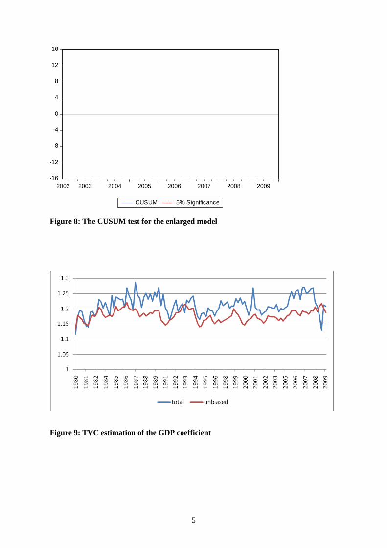
5

-16

-12

-8

-4

0

4

8

12

16

2002 2003 2004 2005 2006 2007 2008 2009

CUSUM 5% Significance Figure 8: The CUSUM test for the enlarged model

Figure 9: TVC estimation of the GDP coefficient

6

0

0.02

0.04

0.06

0.08

0.1

0.12

0.1419

8019

8119

8319

8419

8519

8619

8819

8919

9019

9119

9319

9419

9519

9619

9819

9920

0020

0120

0320

0420

0520

0620

0820

09

total unbiased

Figure 10: TVC estimation of the financial wealth to income ratio

Figure 11: TVC estimation of the housing wealth to income ratio.

7

Figure 12: TVC estimation of the confidence effect

Figure 13 TVC estimation of the interest rate effect