Embed Size (px)
Citation preview

M.AARTHI – AP/CSE Mahalakshmi Engineering College Page 1
DEPARTMENT OF COMPUTER SCIENCE AND ENGINEERING
QUESTION BANK
UNIT-I
SUB CODE: CS2251 DEPT: CSE
SUB NAME: DESIGN AND ANALYSIS OF ALGORITHMS SEM/YEAR: III/ II
PART – A (2 Marks)
1. Compare the order of growth n! and 2n. (AUC DEC 2006)
n- Linear, n! - Factorial function, 2n- exponential function.
The various functions for analysis of algorithms is given below,
n n! 2n
10 3.6x10⁶ 103
102 9.3x10157 1.3x1030
2. What is meant by stepwise refinement? (AUC DEC 2007)
A way of developing a computer program by first describing general functions,
then breaking each function down into details which are refined in successive steps until
the whole program is fully defined. Also called top-down design
3. How is an algorithm’s time efficiency measured? (AUC DEC 2007)
Time efficiency - a measure of amount of time for an algorithm to execute.
Space efficiency - a measure of the amount of memory needed for an algorithm to
execute.
4. How is the efficiency of an algorithm defined? (AUC DEC 2007)
The efficiency of algorithms is the determination of the number of resources ( such as
time and storage) necessary to execute them.
To determine resource consumption:
CPU time
Memory space
Compare different methods for solving the same problem before actually
implementing them and running the programs.
5. What is the use of asymptotic notations? (AUC JUN 2010)

M.AARTHI – AP/CSE Mahalakshmi Engineering College Page 2
The order of growth of the running time of an algorithms, gives a simple
characterization of algorithms efficiently. It also allows comparing relative
performance of alternative algorithms.
For example, when input size is large enough, merge sort, whose worst-case
running time O (n log n) beats insertion sort, whose worst case running time is
O(n2).
Asymptotic notations are methods to estimate and represent efficiency of an
algorithm using simple formula. This useful for separating algorithms that do
drastically different amount of work for large inputs.
6. What are the properties of Big-Oh notation? (AUC JUN 2010/DEC 2011)
(i) If f O(g) and g O(h), then f O(h); that is O is transitive. Also Ω,
7. If 1 0....m
ma n a n a , then prove that f(n)=O(nm). (AUC DEC 2010)
0
0
0
( ) | |
| |
| | 1 ( ) ( ) .
mi
i
i
mm i m
i
i
mm m
i
i
f n a n
n a n
n a for n f n O n wheremis fixed
8. Establish the relationship between O and . (AUC DEC 2010)
If f € O(g) if and only if g € Ω (f)
9. Differentiate Time Complexity and Space Complexity. (AUC MAY 2010)
Time efficiency:
It indicates how fast an algorithm runs.
The running time of an algorithm on a particular input is the number of
primitive operations or steps executed.
Space efficiency:
It deals with extra space the algorithm requires.
Due to technological innovations over the period, space required is not a
much concern, but because of memory hierarchy(where we have faster
main memory, slow secondary memory and cache) this is of prime
importance.
So the general framework for analyzing the efficiency of algorithms includes both time
and space efficiency.
10. What is a Recurrence Equation? (AUC MAY 2010)

M.AARTHI – AP/CSE Mahalakshmi Engineering College Page 3
A recurrence equation is an equation or inequality that describes a function in
terms of its value on smaller inputs.
An equation relating the generic term to one or more other terms of the
sequence, combined with one or more explicit values for the first term(s),e.g.,
x(n)=x(n-1)+n for n>0 ………(1)
x(0)=0 ……….(2)
It is the latter method that is particularly important for analysis of recursive algorithms.
11. Using the step count method analyze the time complexity when 2 m × n
matrices are added. (AUC MAY 2011)
Introduce a variable count in the algorithm Matrix addition is to add two m x n
matrices a and b together.
Algorithm : Add (a,b,c,m,n)
for i:=1 to m do
Count:= count +1; //for ‘for I’
for j=1 to n do
Count:= count +1; // for ‘for j’
C[i , j]= a[ i, j] + b[ i, j ];
Count:=count +1; // for the assignment
Count:=count +1; // For last time of ‘for j’
Count:=count +1; // For last time of ‘for i’
Step count
When analyzing a recursive program to find summation of n numbers, the frequency and
total steps is checked with two conditions that is n=0 (or) n>0. The equivalent recursive
formula is,
tRsum (n)= 2 if n=0
2+ tRsum (n-1) if n>0
M.AARTHI – AP/CSE Mahalakshmi Engineering College Page 4
These recursive formulas are referred to recurrence relations. One way of solving any
recurrence relation is to make repeated substitutions for each occurrence of the function
tRsum on the right hand side until all such occurrences disappear.
tRsum (n)= 2+ tRsum (n-1)
= 2 + 2 + tRsum (n-2)
= 2 (2) + tRsum (n-2)
=n( 2) + tRsum (0)
=2n+2, n>=0
12. An array has exactly n nodes. They are filled from the set 0, 1, 2,...,n-1, n.
There are no duplicates in the list. Design an O(n) worst case time algorithm to
find which one of the elements from the above set is missing in the array. (AUC MAY
2011)
Algorithm:
Find (A[0,…….n])
// Input: An array A[0……n] filled with set values 0,1,2,….,n
// Output: If all the array locations are filled returns 1 else returns -1.
i<- 0
While (i<=n) and (A[i]==i) do
i<- i+1
If i<=n return 1
else
return -1
13. Define Big Oh notation. (AUC MAY 2008/ MAY 2012)
A function t(n) is said to be in O(g(n)), denoted as t(n) € O(g(n)), if t(n) is
bounded above by some constant multiple of g(n) for all large n.i.e., if there exist
some positive constant c and some non- negative integer n0 such that,
t(n) <= cg(n) for all n >=n0
14. What is meant by linear search? (AUC MAY 2012/DEC 2011)
Linear search algorithm is an algorithm which is used to find the location of the
key element x, by checking the successive elements of the array sequentially
one after another from the first location to the end of the array. The element may
or may not in the array. If the match is found then it is called successful search.
Otherwise it is called as unsuccessful search.

M.AARTHI – AP/CSE Mahalakshmi Engineering College Page 5
It returns the first index position if the element exists, otherwise -1 will be
returned( to indicate element not found)
15. Define Notion of Algorithm and characteristics of algorithm.
An Algorithm is a finite set of instructions that, if followed, accomplishes a particular task. In addition, all algorithms should satisfy the following criteria.
1. INPUT Zero or more quantities are externally supplied. 2. OUTPUT At least one quantity is produced. 3. DEFINITENESS Each instruction is clear and unambiguous. 4. FINITENESS If we trace out the instructions of an algorithm, then for all cases, the
algorithm terminates after a finite number of steps. 5. EFFECTIVENESS Every instruction must very basic so that it can be carried out, in
principle, by a person using only pencil & paper.
16. Define best, worst, average case Time Complexity.
Best case:
This analysis constrains on the input, other than size. Resulting in the fasters possible run time
Worst case: This analysis constrains on the input, other than size. Resulting in the fasters possible run time
Average case:
This type of analysis results in average running time over every type of input.
Complexity: Complexity refers to the rate at which the storage time grows as a function of the problem size
17. What is the explicit formula for the nth Fibonacci number?
The formula for the nth Fibonacci number is given by
T(n) = 1/
M.AARTHI – AP/CSE Mahalakshmi Engineering College Page 6
18. Define Smoothness rule. When it is used?
Smooth function are interesting because of the smoothness rule.
Let p<=2 be an integer. Let f be an eventually non-decreasing function.f is m said
to be p-smooth if f(pn)€ O(f(n)).
19. What are the steps that need to be followed while designing and analyzing an algorithm?
1. Understanding the problem.
2. Decision making on
Appropriate Data structure
Algorithm Design Techniques etc.
3. Designing an algorithm
4. Proving the correctness of the algorithm.
5. Proving an Algorithm’s correctness.
6. Analyzing an algorithm.
7. Coding an algorithm.
20. List the Best case, Worst case, Average case computing time of linear search.
The best case for the linear search algorithm arises when the searching element
appears in the first location.
The worst case for the linear search algorithm arises when the searching element
could be either in the last location or could not be in array.
The average case for the linear search algorithm arises when the searching element
appears in the middle of the array.
Best- case Worst-case Average-case
O(1) O(n) O(n)
21. List the types of asymptotic notations.
Three standard notations are used to compare orders of growth of an algorithm basic
operation count.
Big oh: f (n) = O (g (n)): class of functions f (n) that grow no faster than g (n).
Big omega: f (n) = Ω (g (n)): class of functions f(n) that grow at least as fast as g(n).
Theta: f (n) = Ө (g (n)): class of functions f(n) that grow at same rate as g(n). 22. What is conditional Asymptotic notation?
Let f, g: N-> R >=0. It is said that f (n) = O (g (n) | A (n)), read as g (n) when A (n), if there exists two positive constants c € and n0 € N such that A(n) [ f(n) <= cg(n)], for all n>= n0
23. What is the classification of the recurrence equation?

M.AARTHI – AP/CSE Mahalakshmi Engineering College Page 7
Recurrence equation can be classified as follows
1. Homogeneous
2. Inhomogeneous
24. Define Algorithm.
An algorithm is a step-by-step procedure for solving a computational problem in a
finite amount of time.
All algorithms must satisfy its characteristics .An attempt to formalize things as
algorithms leads to a much deeper understanding.
An algorithm is a sequence of unambiguous instructions for solving a computational
problem, i.e., for obtaining a required output for any legitimate input in a finite amount
of time.

M.AARTHI – AP/CSE Mahalakshmi Engineering College Page 8
PART-B (16 Marks)
1. Explain how Time Complexity is calculated. Give an example (16) (AUC,MAY 2010)

M.AARTHI – AP/CSE Mahalakshmi Engineering College Page 9

M.AARTHI – AP/CSE Mahalakshmi Engineering College Page 10

M.AARTHI – AP/CSE Mahalakshmi Engineering College Page 11
2. Elaborate an Asymptotic Notations with example. (16) (AUC MAY 2010/MAY
2011/JUN 2012)

M.AARTHI – AP/CSE Mahalakshmi Engineering College Page 12

M.AARTHI – AP/CSE Mahalakshmi Engineering College Page 13

M.AARTHI – AP/CSE Mahalakshmi Engineering College Page 14

M.AARTHI – AP/CSE Mahalakshmi Engineering College Page 15
3. Explain the process of solving recurrence relations.(16) (AUC JUN 2010)

M.AARTHI – AP/CSE Mahalakshmi Engineering College Page 16

M.AARTHI – AP/CSE Mahalakshmi Engineering College Page 17

M.AARTHI – AP/CSE Mahalakshmi Engineering College Page 18
When an algorithm contains a recursive call to itself, its running time can often be described
by a recurrence.
Recurrence Equation A recurrence relation is an equation that recursively defines a sequence. Each term of the sequence is defined as a function of the preceding terms. A difference equation is a specific type of recurrence relation.
An example of a recurrence relation is the logistic map:
Example: Fibonacci numbers
The Fibonacci numbers are defined using the linear recurrence relation with seed values:
Explicitly, recurrence yields the equations:
We obtain the sequence of Fibonacci numbers which begins: 0, 1, 1, 2, 3, 5, 8, 13, 21, 34, 55, 89, ...
It can be solved by methods described below yielding the closed form expression which
involve powers of the two roots of the characteristic polynomial t2 = t + 1; the generating
function of the sequence is the rational function t / (1 − t − t2).
Substitution method
The substitution method for solving recurrences entails two steps:
1. Guess the form of the solution
2. Use mathematical induction
To find the constants and show that the solution works. The name comes from the
substitution of the guessed answer for the function when the inductive hypothesis is
applied to smaller values.
This method is powerful, but it obviously can be applied only in cases when it is
easy to guess the form of the answer. The substitution method can be used to
establish either upper or lower bounds on a recurrence. As an example, let us
determine an upper bound on the recurrence which is similar to recurrences (4.2)
and (4.3).
We guess that the solution is T (n) = O(n lg n).Our method is to prove that T (n) ≤ cn
lg n for an appropriate choice of the constant c >0. We start by assuming that this
bound holds for ⌊n/2⌋, that is, that T (⌊n/2⌋) ≤ c ⌊n/2⌋ lg(⌊n/2⌋).
Substituting into the recurrence yields
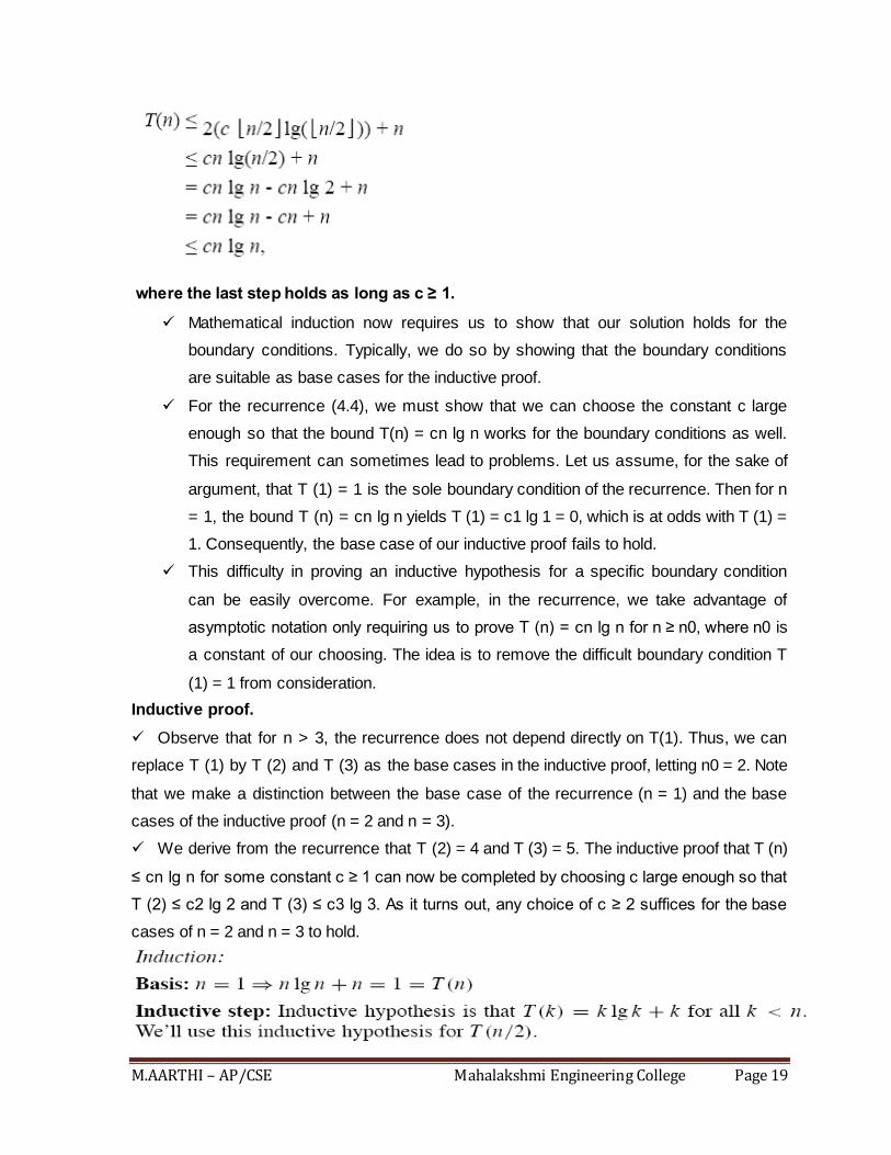
M.AARTHI – AP/CSE Mahalakshmi Engineering College Page 19
where the last step holds as long as c ≥ 1.
Mathematical induction now requires us to show that our solution holds for the
boundary conditions. Typically, we do so by showing that the boundary conditions
are suitable as base cases for the inductive proof.
For the recurrence (4.4), we must show that we can choose the constant c large
enough so that the bound T(n) = cn lg n works for the boundary conditions as well.
This requirement can sometimes lead to problems. Let us assume, for the sake of
argument, that T (1) = 1 is the sole boundary condition of the recurrence. Then for n
= 1, the bound T (n) = cn lg n yields T (1) = c1 lg 1 = 0, which is at odds with T (1) =
1. Consequently, the base case of our inductive proof fails to hold.
This difficulty in proving an inductive hypothesis for a specific boundary condition
can be easily overcome. For example, in the recurrence, we take advantage of
asymptotic notation only requiring us to prove T (n) = cn lg n for n ≥ n0, where n0 is
a constant of our choosing. The idea is to remove the difficult boundary condition T
(1) = 1 from consideration.
Inductive proof.
Observe that for n > 3, the recurrence does not depend directly on T(1). Thus, we can
replace T (1) by T (2) and T (3) as the base cases in the inductive proof, letting n0 = 2. Note
that we make a distinction between the base case of the recurrence (n = 1) and the base
cases of the inductive proof (n = 2 and n = 3).
We derive from the recurrence that T (2) = 4 and T (3) = 5. The inductive proof that T (n)
≤ cn lg n for some constant c ≥ 1 can now be completed by choosing c large enough so that
T (2) ≤ c2 lg 2 and T (3) ≤ c3 lg 3. As it turns out, any choice of c ≥ 2 suffices for the base
cases of n = 2 and n = 3 to hold.

M.AARTHI – AP/CSE Mahalakshmi Engineering College Page 20
For most of the recurrences we shall examine, it is straightforward to extend boundary
conditions to make the inductive assumption work for small n.
The iteration method
The method of iterating a recurrence doesn't require us to guess the answer, but it
may require more algebra than the substitution method. The idea is to expand
(iterate) the recurrence and express it as a summation of terms dependent only on n
and the initial conditions. Techniques for evaluating summations can then be used
to provide bounds on the solution.
As an example, consider the recurrence T(n) = 3T(n/4) + n.
We iterate it as follows:
T(n) = n + 3T(n/4)
= n + 3 (n/4 + 3T(n/16))
= n + 3(n/4 + 3(n/16 + 3T(n/64)))
= n + 3 n/4 + 9 n/16 + 27T(n/64),
where n/4/4 = n/16 and n/16/4 = n/64 follow from the identity (2.4).
How far must we iterate the recurrence before we reach a boundary condition? The
ith term in the series is 3i n/4i. The iteration hits n = 1 when n/4i = 1 or, equivalently,
when i exceeds log4 n. By continuing the iteration until this point and using the
bound n/4i n/4i, we discover that the summation contains a decreasing geometric
series:

M.AARTHI – AP/CSE Mahalakshmi Engineering College Page 21
The master method
The master method provides a "cookbook" method for solving recurrences of the
form where a ≥ 1 and b > 1 are constants and f (n) is an asymptotically positive
function. The master method requires memorization of three cases, but then the
solution of many recurrences can be determined quite easily, often without pencil
and paper.
The recurrence describes the running time of an algorithm that divides a problem of
size n into a sub problems, each of size n/b, where a and b are positive constants.
The a sub problems are solved recursively, each in time T (n/b). The cost of dividing
the problem and combining the results of the sub problems is described by the
function f (n). (That is, using the notation from, f(n) = D(n)+C(n).) For example, the
recurrence arising from the MERGE-SORT procedure has a = 2, b = 2, and f (n) =
Θ(n).
As a matter of technical correctness, the recurrence isn't actually well defined
because n/b might not be an integer. Replacing each of the a terms T (n/b) with
either T (⌊n/b⌋) or T (⌈n/b⌉) doesn't affect the asymptotic behavior of the recurrence,
however. We normally find it convenient, therefore, to omit the floor and ceiling
functions when writing divide-and- conquer recurrences of this form.
4. What is linear search? Analyze linear search in terms of its time and space complexity.(16)
(AUC JUN 2010 /MAY 2011)
Explain how analysis of linear search is done with a suitable illustration. (10)(AUC DEC 2011)
Linear Search, as the name implies is a searching algorithm which obtains its result
by traversing a list of data items in a linear fashion. It will start at the beginning of a
list, and mosey on through until the desired element is found, or in some cases is
not found.
The aspect of Linear Search which makes it inefficient in this respect is that if the
element is not in the list it will have to go through the entire list. As you can imagine
this can be quite cumbersome for lists of very large magnitude, keep this in mind as
you contemplate how and where to implement this algorithm.

M.AARTHI – AP/CSE Mahalakshmi Engineering College Page 22
Of course conversely the best case for this would be that the element one is
searching for is the first element of the list, this will be elaborated more so in the
―Analysis & Conclusion
Linear Search Steps:
Step 1 - Does the item match the value I‟m looking for? Step 2 - If it does match return, you‟ve
found your item!
Step 3 - If it does not match advance and repeat the process.
Step 4 - Reached the end of the list and still no value found? Well obviously the item is not in
the list! Return -1 to signify you have not found your value.
As always, visual representations are a bit more clear and concise so let me present one
for you now. Imagine you have a random assortment of integers for this list:
Legend:
- The key is blue
- The current item is green.
- Checked items are red
Ok so here is our number set, my lucky number happens to be 7 so let„s put this value
as the key, or the value in which we hope Linear Search can find. Notice the indexes of
the array above each of the elements, meaning this has a size or length of 5. I digress
let us look at the first term at position 0. The value held here 3, which is not equal to 7.
We move on.
--0 1 2 3 4 5 [ 3 2 5 1 7 0 ]
So we hit position 0, on to position 1. The value 2 is held here. Hmm still not equal to 7. We
march on.
--0 1 2 3 4 5 [ 3 2 5 1 7 0 ]
Position 2 is next on the list, and sadly holds a 5, still not the number we„re looking for.
Again we move up one. --0 1 2 3 4 5 [ 3 2 5 1 7 0 ]
Now at index 3 we have value 1. Nice try but no cigar let„s move forward yet again.
--0 1 2 3 4 5 [ 3 2 5 1 7 0 ]
Ah Ha! Position 4 is the one that has been harboring 7, we return the position in the array which
holds 7 and exit.
--0 1 2 3 4 5 [ 3 2 5 1 7 0 ]
As you can tell, the algorithm may work find for sets of small data but for incredibly large
data sets I don„t think I have to convince you any further that this would just be
downright inefficient to use for exceeding large sets. Again keep in mind that Linear

M.AARTHI – AP/CSE Mahalakshmi Engineering College Page 23
Search has its place and it is not meant to be perfect but to mold to your situation that
requires a search.
Also note that if we were looking for let’s say 4 in our list above (4 is not in the set) we
would traverse through the entire list and exit empty handed. I intend to do a tutorial on
Binary Search which will give a much better solution to what we have here however it
requires a special case.
//linearSearch Function
int linearSearch(int data[], int length, int val)
for (int i = 0; i <= length; i++) if (val == data[i])
return i; //end if
//end for
return -1; //Value was not in the list //end linearSearch Function
Analysis & Conclusion
As we have seen throughout this tutorial that Linear Search is certainly not the absolute
best method for searching but do not let this taint your view on the algorithm itself. People
are always attempting to better versions of current algorithms in an effort to make existing
ones more efficient. Not to mention that Linear Search as shown has its place and at the
very least is a great beginner’s introduction into the world of searching algorithms. With this
is mind we progress to the asymptotic analysis of the Linear Search:
Worst Case:
The worst case for Linear Search is achieved if the element to be found is not in the list at all.
This would entail the algorithm to traverse the entire list and return nothing. Thus the worst case
running time is: O(n).
Average Case:
The average case is in short revealed by insinuating that the average element would be
somewhere in the middle of the list or N/2. This does not change since we are dividing by a
constant factor here, so again the average case would be:
O(n).
Best Case:
The best case can be a reached if the element to be found is the first one in the list. This would
not have to do any traversing spare the first one giving this a constant time complexity is:
O (1).
5. Explain briefly the Time Complexity estimation, space complexity estimation and the
tradeoff between Time and Space Complexity.(6) (AUC DEC 2010)

M.AARTHI – AP/CSE Mahalakshmi Engineering College Page 24

M.AARTHI – AP/CSE Mahalakshmi Engineering College Page 25

M.AARTHI – AP/CSE Mahalakshmi Engineering College Page 26

M.AARTHI – AP/CSE Mahalakshmi Engineering College Page 27

M.AARTHI – AP/CSE Mahalakshmi Engineering College Page 28
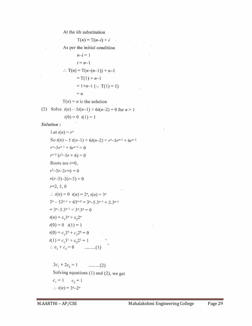
6. Solve the following recurrence equations completely. (AUC DEC 2010)
(i) 1
1
( ) ( ) , 2n
i
T n T i if n T(n)=1, if n=1. (4)
(ii) ( ) 5 ( 1) 6 ( 2)T n T n T n . (3)
(iii) ( ) 2 ( ) log2
nT n T n n . (3)
Solution:
(i) 1
1
( ) ( ) , 2n
i
T n T i if n T(n)=1, if n=1. (4)
M.AARTHI – AP/CSE Mahalakshmi Engineering College Page 29

M.AARTHI – AP/CSE Mahalakshmi Engineering College Page 30
7. Write the linear search algorithm and analyze for its best, worst, average case time
complexity. (10)
(AUC DEC 2010)

M.AARTHI – AP/CSE Mahalakshmi Engineering College Page 31

M.AARTHI – AP/CSE Mahalakshmi Engineering College Page 32

M.AARTHI – AP/CSE Mahalakshmi Engineering College Page 33
8. Prove that for any two functions f(n) and g(n), we have ( ) ( ( ))f n g n if and only if
( ) ( ( ))f n g n and (6) (AUC DEC
2010)
9. Define Asymptotic notations. Distinguish between Asymptotic notation and conditional
asymptotic notation. (10) (AUC DEC 2011)
10. Explain how the removing condition is done from the conditional asymptotic notation with an
example. (6) (AUC DEC 2011)
Many algorithms are easier to analyze if initially we restrict our attention to instances
whose size satisfies a certain condition, such as being a power of 2. Consider, for
example, the divide and conquer algorithm for multiplying large integers that we saw
in the Introduction. Let n be the size of the integers to be multiplied.
The algorithm proceeds directly if n = 1, which requires a microseconds for an
appropriate constant a. If n>1, the algorithm proceeds by multiplying four pairs of
integers of size n/2 (or three if we use the better algorithm).
Moreover, it takes a linear amount of time to carry out additional tasks. For
simplicity, let us say that the additional work takes at most bn microseconds for an
appropriate constant b.
REMOVING CONDITIONS FROM CONDITIONAL ASYMPTOTIC NOTATIONS
Temporal comparison is not the only issue in algorithms. There are space issues as well.
Generally, a tradeoff between time and space is noticed in algorithms. Asymptotic
notation empowers you to make that trade off.
If you think of the amount of time and space your algorithm uses as a function of your
data over time or space (time and space are usually analyzed separately), you can
analyze how the time and space is handled when you introduce more data to your
program.

M.AARTHI – AP/CSE Mahalakshmi Engineering College Page 34
This is important in data structures because you want a structure that behaves efficiently
as you increase the amount of data it handles. Keep in mind though those algorithms
that are efficient with large amounts of data are not always simple and efficient for small
amounts of data.
So if you know you are working with only a small amount of data and you have concerns
for speed and code space, a trade off can be made for a function that does not behave
well for large amounts of data.
A few examples of asymptotic notation
Generally, we use asymptotic notation as a convenient way to examine what can happen in a
function in the worst case or in the best case. For example, if you want to write a function that
searches through an array of numbers and returns the smallest one:
function find-min(array a[1..n])
let j :=
for i := 1 to n:
j := min(j, a[i])
repeat
return j
end
Regardless of how big or small the array is, every time we run find-min, we have to
initialize the i and j integer variables and return j at the end. Therefore, we can just think
of those parts of the function as constant and ignore them.
So, how can we use asymptotic notation to discuss the find-min function? If we search
through an array with 87 elements, then the for loop iterates 87 times, even if the very
first element we hit turns out to be the minimum. Likewise, for elements, the for loop
iterates times. Therefore we say the function runs in time .
What about this function:
function find-min-plus-max(array a[1..n])
// First, find the smallest element in the array
let j := ;
for i := 1 to n:
j := min(j, a[i])
repeat
let minim := j
// Now, find the biggest element, add it to the smallest and

M.AARTHI – AP/CSE Mahalakshmi Engineering College Page 35
j := ;
for i := 1 to n:
j := max(j, a[i])
repeat
let maxim := j
// return the sum of the two
return minim + maxim;
end
11. Define recurrence equation and explain how solving recurrence equations are done. (6)
(AUC DEC 2011)
12. With a suitable example, explain the method of solving recurrence equations.(16)
(AUC JUN 2012)
13. Write and solve the recurrence relation of Tower of Hanoi puzzle. (16) (AUC NOV 2013)
Certain bacteria divide into two bacteria every second. It was noticed that when one
bacterium is placed in a bottle, it fills it up in 3 minutes. How long will it take to fill half the
bottle?
Many processes lend themselves to recursive handling. Many sequences are
determined by previous members of the sequence. How many got the bacteria process
right?
If we denote the number of bacteria at second number k by bk then we have: bk+1 = 2bk
, b1 = 1.
This is a recurrence relation.
Another example of a problem that lends itself to a recurrence relation is a famous
puzzle: The towers of Hanoi
This puzzle asks you to move the disks from the left tower to the right tower, one disk at a
time so that a larger disk is never placed on a smaller disk. The goal is to use the smallest

M.AARTHI – AP/CSE Mahalakshmi Engineering College Page 36
number of moves. Clearly, before we move the large disk from the left to the right, all but
the bottom disk, have to be on the middle tower. So if we denote the smallest number of
moves by hn then we have: hn+1 = 2hn + 1
A simple technic for solving recurrence relation is called telescoping.
Start from the first term and sequentially produce the next terms until a clear pattern
emerges. If you want to be mathematically rigorous you may use induction.
Solving bn+1 = 2bn; b1 = 1.
b1 = 1; b2 = 2; b3 = 4; : : : bn = 2n-1.
Solving the Towers of Hanoi recurrence relation:
h1 = 1; h2 = 3; h3 = 7; h4 = 15; : : : hn = 2n - 1
Proof by induction:
step 1 h1 = 1 = 21 -1
step 2 Assume hn = 2n - 1
step 3 Prove: hn+1 = 2n+1 -1.
step 4 hn+1 = 2hn + 1 = 2(2n -1) + 1 = 2n+1 - 1.
step 5 Solve: an = 1/ 1+an-1, a1 = 1.
Telescoping yields: 1,1/ 2, 2 / 3, 3/ 5, 5/ 8, 8/ 13

M.AARTHI – AP/CSE Mahalakshmi Engineering College Page 37

M.AARTHI – AP/CSE Mahalakshmi Engineering College Page 38

M.AARTHI – AP/CSE Mahalakshmi Engineering College Page 39
Coding Towers of Hanoi
Now that we know how to solve an n -disc problem, let's turn this into an algorithm
we can use.
If there is one disc, then we move 1 disc from the source pole to the destination
pole. Otherwise, we move n - 1 discs from the source pole to the temporary pole, we
move 1 disc from the source pole to the destination pole, and we finish by moving
the n - 1 discs from the temporary pole to the destination pole.
void TOH(int n, int p1, int p2, int p3)
if (n == 1) printf("Move top disc from %d to %d.\n", p1, p2);
else
TOH(n-1, p1, p3, p2);
printf("Move top disc from %d to %d.\n", p1, p2);
TOH(n-1, p3, p2, p1);
M.AARTHI – AP/CSE Mahalakshmi Engineering College Page 40
Of course, we can simplify this to the following:
void TOH(int n, int p1, int p2, int p3)
if (n>1) TOH(n-1, p1, p3, p2);
printf("Move top disc from %d to %d.\n", p1, p2);
if (n>1) TOH(n-1, p3, p2, p1);
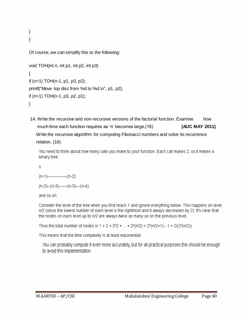
14. Write the recursive and non-recursive versions of the factorial function. Examine how
much time each function requires as ‘n’ becomes large.(16) (AUC MAY 2011)
Write the recursive algorithm for computing Fibonacci numbers and solve its recurrence
relation. (16)

M.AARTHI – AP/CSE Mahalakshmi Engineering College Page 41

M.AARTHI – AP/CSE Mahalakshmi Engineering College Page 42
15. Explain the master method with an example.

M.AARTHI – AP/CSE Mahalakshmi Engineering College Page 43

M.AARTHI – AP/CSE Mahalakshmi Engineering College Page 44
16. Describe the steps in analyzing and coding of an algorithm.(8)
Informally, an algorithm is any well-defined computational procedure that takes some value, or set of values, as input and produces some value, or set of values, as output. An algorithm is thus a sequence of computational steps that transform the input into the output.
Characteristics of Algorithms:
While designing an algorithm as a solution to a given problem, we must take care of the following five important characteristics of an algorithm. 1. Finiteness 2. Definiteness 3. Inputs 4. Output 5. Effectiveness