S1

Electronic Supplementary Information (ESI) for:

Delayed Vibrational Modulation of the Solvated GFP

Chromophore into a Conical Intersection

Miles A. Taylor,†,¶ Liangdong Zhu,†,‡,¶ Nikita D. Rozanov,†,§ Kenneth T. Stout,†,§ Cheng Chen,†

and Chong Fang*,†,‡

†Department of Chemistry, Oregon State University, 153 Gilbert Hall, Corvallis, Oregon, 97331-4003, United States

‡Department of Physics, Oregon State University, 301 Weniger Hall, Corvallis, Oregon, 97331-6507, United States

§School of Chemical, Biological and Environmental Engineering, 116 Johnson Hall, Corvallis, Oregon, 97331-8618, United States

¶M.A.T. and L.Z. contributed equally to this work.

*To whom correspondence may be addressed. E-mail: Chong.Fang@oregonstate.edu.

Electronic Supplementary Material (ESI) for Physical Chemistry Chemical Physics.This journal is © the Owner Societies 2019

S2

Table of Contents Page number

ESI Text S3 – 6

Further Motivation to Study the GFP Model Chromophore in Solution S3 – 5

Solvent Dependence of Mode Frequencies Aids Vibrational Assignment S5 – 6

ESI Figures S7 – 19

Figure S1. Steady-state electronic spectroscopy of anionic HBDI in aqueous solution S7

Figure S2. Ground state Raman spectrum and mode assignment of anionic HBDI S8 – 9

Figure S3. Transient absorption and probe-wavelength-dependent dynamic plots S10 – 11

Figure S4. Global analysis and time constants of transient absorption spectra S12

Figure S5. Semi-automatic baselines of the time-resolved excited state FSRS S13

Figure S6. Early-time dynamics of the 866 cm-1 marker band in S1 of anionic HBDI S14

Figure S7. Representative FSRS spectra at late time delays S15 – 16

Figure S8. Coherent residual plot for 2D-FSRS of the anionic HBDI in aqueous solution without and with 50% (v/v) glycerol S17

Figure S9. 2D-FSRS plot of the anionic HBDI in aqueous solution with 50% (v/v) glycerol S18 – 19

Additional discussion follows each figure caption

ESI Tables S20 – 25

Table S1. Transient absorption dynamics of the anionic HBDI in aqueous solution S20

Table S2. Excited state Raman peak intensity dynamics and mode assignment for the anionic HBDI in aqueous solution without and with 50% (v/v) glycerol S21 – 23

Table S3. Frequency shift trend of three Raman marker bands and other key properties as a function of the chromophore ring twisting dihedral angle S24 – 25

ESI References S26 – 29

S3

ESI Text

Further Motivation to Study the GFP Model Chromophore in Solution. In this work, we aim

to track the atomic choreography of the green fluorescent protein (GFP) chromophore analogue

p-HBDI in basic aqueous solution using the newly developed wavelength-tunable femtosecond

stimulated Raman spectroscopy (FSRS, see main text). This methodology allows us to provide

novel insights into the “dark secrets” of HBDI during its photoinduced isomerization in solution

instead of highly efficient radiative emission (e.g., fluorescence) in a protein matrix. Previous

ultrafast electronic spectroscopy by Meech, Tonge, van Grondelle, Larsen, et al.1-3 has revealed

the following molecular insights: (1) there exists a conical intersection (CI) that enables efficient

radiationless internal conversion from S1 to S0, essentially a molecular “funnel” for de-excitation,

(2) the radiationless process is not viscosity controlled with large-scale intramolecular

reorganization, and (3) the ultrafast internal conversion is an intrinsic property of the

chromophore skeleton that could be affected by the local microenvironment including charge

distribution or H-bonding. Later, Gepshtein, Huppert and Agmon described active modes leading

to facile internal conversion not readily retrievable from the time-resolved fluorescence

measurements, and the importance of nonlocal, multi-point twisting motions for the

chromophore with an intrinsic conformational distribution that can manifest inhomogeneous

kinetics (e.g., excited state decay, conformational relaxation) in solution environment.4

In contrast, when inside a protein matrix such as GFP, internal water molecules may provide

further H-bonding, stabilization, and structural constraints for the embedded chromophore,

restricting the rotational freedom of the distal phenolic ring.5-7 Despite the internal conversion

(S1®S0) of its protonated chromophore on ~200 ps timescale due to its rotationally symmetrical

phenolic C–O bond along the proposed rotational axis6,8 (i.e., the adjacent bridging C–C bond,

S4

see Figure 1b for the chemical structure of HBDI chromophore), the highly effective excited

state proton transfer (ESPT) leads to bright green fluorescence from the lower electronic state

corresponding to a deprotonated chromophore. This is an excellent example of ESPT-facilitated

radiative emission outpacing radiationless loss channels, and the H-bonding chain connects the

phenolic hydroxyl group to internal water molecules and protein residues along the well-defined

ESPT chain, which plays a central role in photochemistry of the chromophore.7,9

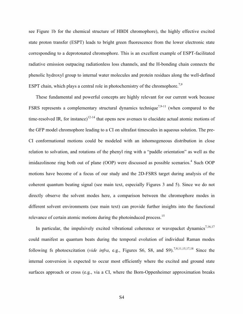
These fundamental and powerful concepts are highly relevant for our current work because

FSRS represents a complementary structural dynamics technique7,9-11 (when compared to the

time-resolved IR, for instance)12-14 that opens new avenues to elucidate actual atomic motions of

the GFP model chromophore leading to a CI on ultrafast timescales in aqueous solution. The pre-

CI conformational motions could be modeled with an inhomogeneous distribution in close

relation to solvation, and rotations of the phenyl ring with a “paddle orientation” as well as the

imidazolinone ring both out of plane (OOP) were discussed as possible scenarios.4 Such OOP

motions have become of a focus of our study and the 2D-FSRS target during analysis of the

coherent quantum beating signal (see main text, especially Figures 3 and 5). Since we do not

directly observe the solvent modes here, a comparison between the chromophore modes in

different solvent environments (see main text) can provide further insights into the functional

relevance of certain atomic motions during the photoinduced process.15

In particular, the impulsively excited vibrational coherence or wavepacket dynamics7,16,17

could manifest as quantum beats during the temporal evolution of individual Raman modes

following fs photoexcitation (vide infra, e.g., Figures S6, S8, and S9).7,9,11,15,17,18 Since the

internal conversion is expected to occur most efficiently where the excited and ground state

surfaces approach or cross (e.g., via a CI, where the Born-Oppenheimer approximation breaks

S5

down), the chromophore intramolecular twisting motions seem to play an important role in the

electronically excited state. In other words, an effective CI usually involves a large vibronic

coupling between electronic states (e.g., S1 and S0) hence supporting an ultrafast crossing

process.19-21 That way we can elucidate the interplay among the rupture of ground-state extended

conjugation upon electronic excitation, intramolecular charge transfer, and ring twisting motions,

thus providing a fundamental understanding of the photoinduced reactions of ring-conjugated

molecular systems, also leading to future design of molecular machines with new functions. This

mechanism coupled with recent engineering effort9,22-24 is particularly relevant due to the

continuing and burgeoning interest of GFP fluorescence from an interdisciplinary context from

molecular spectroscopy, physical chemistry, bioorganic chemistry, biophysics, bioimaging,

bioengineering, nanophotonics to optogenetics.

Solvent Dependence of Mode Frequencies Aids Vibrational Assignment. The isolated

chromophore in solution is not really “isolated” per se, and the Raman spectrum contains

detailed information about vibrational motions. The spectral shift of vibrational bands in

different solvents is a clear indication that the chromophore is not only surrounded by solvent

molecules, but also forming specific hydrogen bonds with them. Based on a series of ground-

state FSRS measurements previously performed at UC Berkeley with an 800 nm Raman pump,7

the phenolic C─O stretch frequency of the neutral HBDI chromophore is 1230 and 1228 cm-1 in

CH3OH and CH3CN, respectively. This mode blue shifts to 1241 and 1242 cm-1 for the anionic

chromophore in CH3OH and CH3CN (both with 5% (v/v) 1 M NaOH), respectively, indicating

the departure of the phenolic proton and increase of the phenolic C─O double-bond character.

Upon 400 nm photoexcitation, the 1241 cm-1 mode blue shifts to 1264 cm-1 within the cross-

S6

correlation time of ~130 fs,7 and the excited state mode intensity decays biexponentially with

time constants of ~290 fs (89%) and 1 ps (11%). The difference between the longer time constant

of 1 ps (herein) and 2.9 ps (Table S2) arises from the variation in solvents (methanol vs. water)

and the Raman pump wavelengths (794 nm vs. 550 nm) being used. Further comparisons can be

made between water and the water-glycerol solution, because the latter environment should

effectively lengthen the conformational transition from the initially excited coplanar

chromophore to a twisted one. Modest effect on the observed structural dynamics may infer

some volume-conserving twisting motions.1,4 Nevertheless, the overall trend corroborates the

photoinduced ultrafast isomerization of the anionic HBDI chromophore in solution.

Due to a similar electron redistribution as the chromophore protonation state changes, the

observed imidazolinone ring C=N stretching with some exocyclic C=C stretching motion at 1568

and 1567 cm-1 of the neutral chromophore redshifts to 1558 and 1557 cm-1 of the anionic

chromophore in CH3OH and CH3CN, respectively.

The higher-frequency mode in association with the bridge C=C and phenol ring C=C

stretching motions at 1645 and 1650 cm-1 of the neutral chromophore redshifts to 1634 and 1635

cm-1 of the anionic chromophore in CH3OH and CH3CN, respectively. In particular, the observed

lower mode frequency (i.e., 1645<1650, 1634<1635) is in accord with a larger quantum “box”

due to more effective H-bonding in methanol than that in acetonitrile. These solvent-dependent

Raman mode frequencies provide additional support for the vibrational assignment listed below

for the anionic HBDI chromophore in water (see Figure S2).

S7

ESI Figures

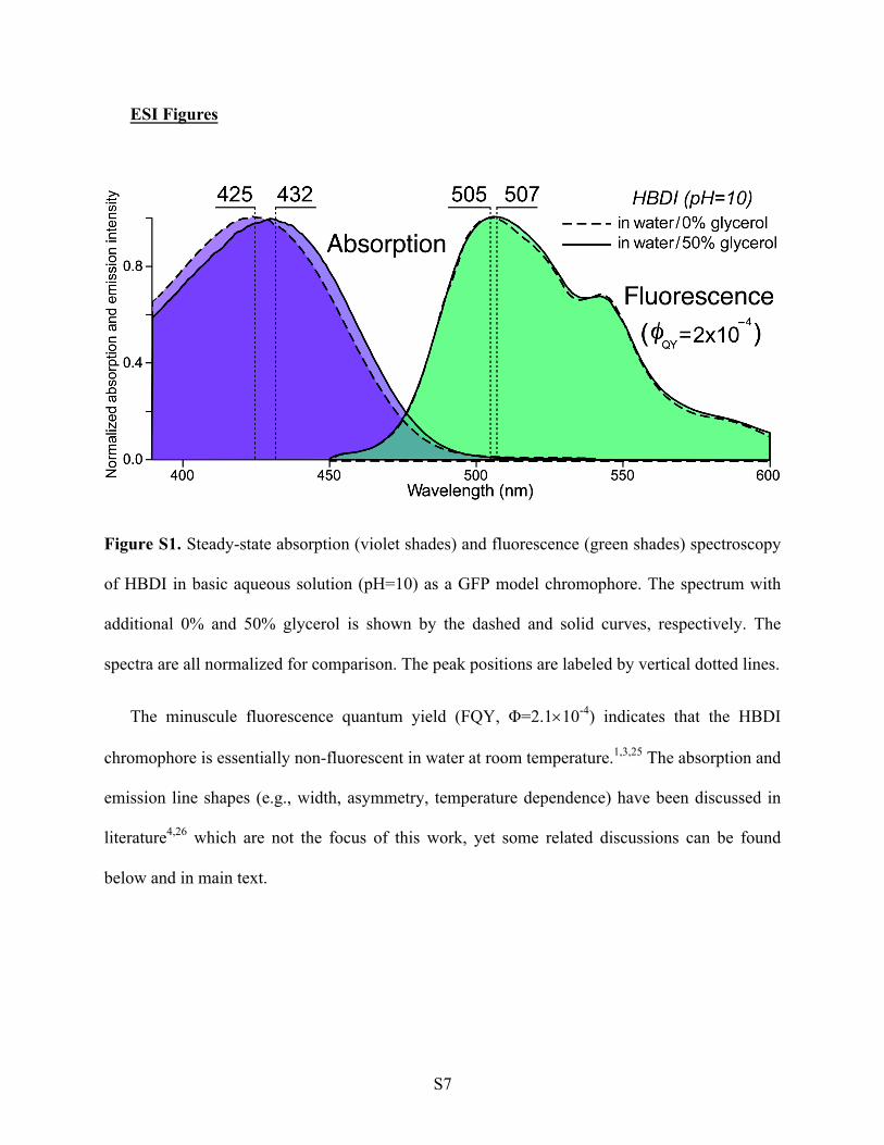
Figure S1. Steady-state absorption (violet shades) and fluorescence (green shades) spectroscopy

of HBDI in basic aqueous solution (pH=10) as a GFP model chromophore. The spectrum with

additional 0% and 50% glycerol is shown by the dashed and solid curves, respectively. The

spectra are all normalized for comparison. The peak positions are labeled by vertical dotted lines.

The minuscule fluorescence quantum yield (FQY, Φ=2.1´10-4) indicates that the HBDI

chromophore is essentially non-fluorescent in water at room temperature.1,3,25 The absorption and

emission line shapes (e.g., width, asymmetry, temperature dependence) have been discussed in

literature4,26 which are not the focus of this work, yet some related discussions can be found

below and in main text.

S8

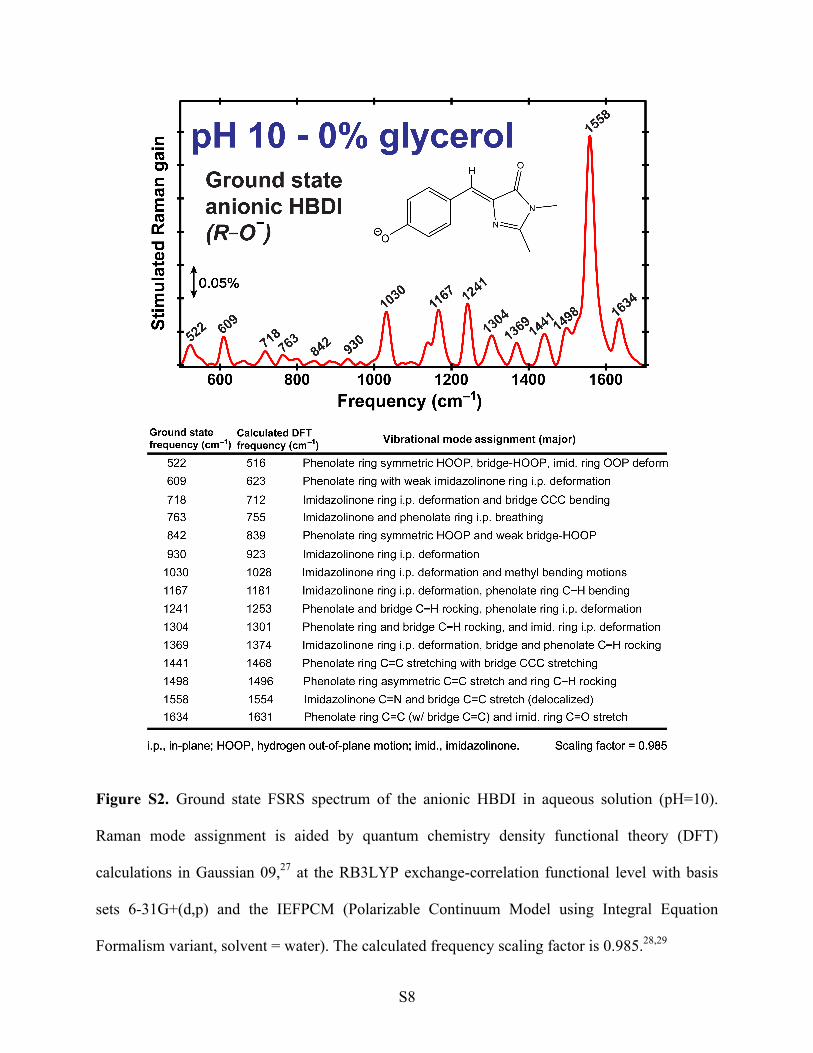
Figure S2. Ground state FSRS spectrum of the anionic HBDI in aqueous solution (pH=10).

Raman mode assignment is aided by quantum chemistry density functional theory (DFT)

calculations in Gaussian 09,27 at the RB3LYP exchange-correlation functional level with basis

sets 6-31G+(d,p) and the IEFPCM (Polarizable Continuum Model using Integral Equation

Formalism variant, solvent = water). The calculated frequency scaling factor is 0.985.28,29

S9

In order to elucidate key structural motions leading to a conical intersection on ultrafast

timescales, we need to study a system with an ideally unidirectional reaction coordinate, without

major competing pathways. For the GFP model chromophore in aqueous solution, we tune the

pH to 10 which is ~2 units above the pKa at the phenolic hydroxyl site30-32 so the anionic

chromophore is the predominant species. In addition to the resultant absence of excited state

proton transfer (ESPT), the higher sensitivity of the anionic chromophore (than the neutral

chromophore) to surrounding solvent molecules arises from solvent stabilization of the negative

charge on the phenolic oxygen.33-35 We also observed a consistent 10–20 cm-1 mode frequency

redshift of the bands above 1550 cm-1 in the anionic form when compared to the neutral form.31

Notably, these vibrational marker bands show a similar pattern for the HBDI chromophore in

solution and protein environment,31 indicating that the pre-resonance Raman enhancement is

mainly applicable for the light-absorbing chromophore not the surrounding protein residues. The

protein matrix confinement effect is especially pronounced on low-frequency vibrational modes

of the embedded chromophore. One would imagine that whether the chromophore is attached to

protein backbone or not, the autocyclic three-residue serine-tyrosine-glycine (SYG, see Figure 1a)

chromophore should contain many similar vibrational modes across the conjugated two-ring

structure. However, within the protein at thermal equilibrium and electronic ground state, the

chromophore is effectively locked into a cis conformation due to limited flexibility from the

surrounding H-bonding network and protein residues, which could suppress the intensity of the

out-of-plane (OOP) modes but not so much for the in-plane modes. This notable difference in

local environment presents itself in the Raman spectrum of HBDI in solution below ~1000 cm-1:

the lower frequency OOP modes exhibit relatively stronger intensity than the higher frequency

in-plane vibrational modes. Inside the protein pocket, such a trend is largely reversed.8,36

S10

Figure S3. Steady-state and time-resolved electronic spectroscopy of the GFP model

chromophore in solution. (a) Transient absorption of anionic HBDI in pH=10 aqueous solution

after 400 nm photoexcitation. Representative spectra at time delay of 0 fs, 400 fs, 1.4 ps, 3.5 ps,

and 200 ps are shown in black, violet, orange red, green, and brown yellow traces, respectively.

Characteristic regions for spectral signal integration and dynamic plot are highlighted by blue

and red rectangular boxes which correspond to (c) and (d), respectively. (b) Steady-state

UV/Visible absorption (cyan) and spontaneous emission spectrum with 390 nm excitation

(orange). The latter spectrum from the essentially non-fluorescent HBDI in water at room

temperature is multiplied by ~80 at this experimental condition to compare with the former

spectrum. (c) Integrated plot of the dominant stimulated emission signal from 524—526 nm at

time delay points of 0—100 ps after 400 nm photoexcitation. The least-squares fit in dashed line

(black) is overlaid with data points (blue) and the associated time constants are noted by the

arrows. The semi-logarithmic plot is shown in the inset to highlight the early-time dynamics. (d)

The integrated plot of the dominant excited state absorption signal from 475—477 nm at time

S11

delay points of 0—100 ps after 400 nm photoexcitation. With the same format as (c), the least-

squares fit in dashed line (black) is overlaid with data points (red triangles) in main plot and with

early-time data points (red circles) in the inset, respectively.

The small fluorescence shoulder peak at ~550 nm in Figure S3b may indicate an additional

radiative emission pathway from the chromophore in the electronic excited state, which was less

resolved in a previous study on the fluorescence peak shape of the anionic p-HBDI chromophore

from 122–298 K.26 The subtle difference from an inhomogeneously broadened fluorescence

spectrum requires further investigation, which is underway in our lab to provide more details

about the electronic excited state potential energy surface (PES) of anionic HBDI in aqueous

solution. The existence of an intermediate electronic state with charge-separated character is

corroborated by the broadness of the SE band at early times24 (Figure S3a) with the transient

ESA band dynamics shown in Figure S3d, which could involve characteristic nuclear motions of

solute molecules surrounded by the highly labile solvent molecules (water in the current work).

S12

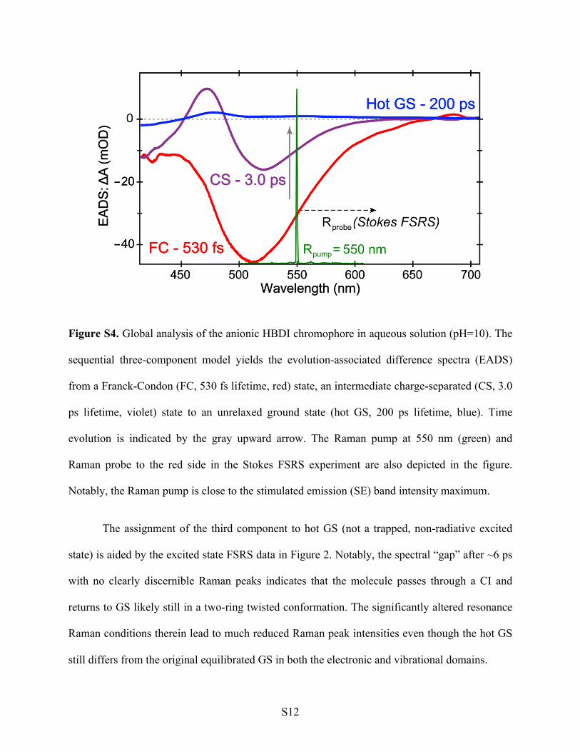
Figure S4. Global analysis of the anionic HBDI chromophore in aqueous solution (pH=10). The

sequential three-component model yields the evolution-associated difference spectra (EADS)

from a Franck-Condon (FC, 530 fs lifetime, red) state, an intermediate charge-separated (CS, 3.0

ps lifetime, violet) state to an unrelaxed ground state (hot GS, 200 ps lifetime, blue). Time

evolution is indicated by the gray upward arrow. The Raman pump at 550 nm (green) and

Raman probe to the red side in the Stokes FSRS experiment are also depicted in the figure.

Notably, the Raman pump is close to the stimulated emission (SE) band intensity maximum.

The assignment of the third component to hot GS (not a trapped, non-radiative excited

state) is aided by the excited state FSRS data in Figure 2. Notably, the spectral “gap” after ~6 ps

with no clearly discernible Raman peaks indicates that the molecule passes through a CI and

returns to GS likely still in a two-ring twisted conformation. The significantly altered resonance

Raman conditions therein lead to much reduced Raman peak intensities even though the hot GS

still differs from the original equilibrated GS in both the electronic and vibrational domains.

S13

Figure S5. Semi-automatic baselines of the time-resolved FSRS using an asymmetric least-

squares algorithm in R software (for statistical computing and graphics). The experimental raw

data traces of photoexcited HBDI chromophore in aqueous solution (pH=10) at representative

time delay points are shown in black and the baselines in red. The stimulated Raman gain

magnitude of 0.1% is depicted by the vertical double-arrowed line. Three excited-state (ES)

maker bands discussed in the main text are labeled and highlighted by the gray dashed lines.

Notably due to the pre-resonantly enhanced Raman peaks by the 550 nm Raman pump (close

to the SE band max), the spline baselines semi-automatically drawn or manually drawn yield no

appreciable differences for the ES Raman peaks and the ensuing spectral data analysis. At early

times when the ES-FSRS signal is the strongest, the spectral dip due to the ground-state bleach

(off-resonance) is very small in comparison. Therefore, the GS addback is not necessary at early

times or it introduces minimal impact to the excited-state peak analysis (e.g., Figure 2, Table 1).

S14

Figure S6. Early-time dynamics of the 866 cm-1 mode in the electronic excited state of anionic

HBDI in pH=10 aqueous solution. (a) Integrated peak intensity plot of the specific Raman band

of interest up to 20 ps after 400 nm photoexcitation. Coherent quantum beating is apparent,

which corresponds to the oscillatory component on top of the incoherent biexponential fit (black

curve, time constants noted). (b) FT intensity plot of the oscillations reveals three modulating

modes at ~231, 47, and 142 cm-1 in the order of decreasing prominence (see Figure 5a for their

time dependence). (c) Peak frequency plot up to 10 ps following photoexcitation with the least-

squares biexponential fit (time constants noted). Some oscillations are present from 0–2 ps but

less obvious than the intensity oscillations in (a), which may be due to the broad peak width in

the excited state and the resultant uncertainty of determining the peak center frequency.

S15

Figure S7. Representative late-time FSRS spectra of anionic HBDI in pH=10 aqueous solution

after ground state (GS) addback. Prominent Raman peaks are labeled by vertical dashed lines,

which represent a redshift from the corresponding peaks in the original ground state (violet,

scaled and plotted for comparison). The addback ratio of the ground state spectrum is denoted in

green on the left side by each transient spectral trace up to 100 ps after 400 nm photoexcitation.

The orange arrow highlights the gradual blueshift of the transient Raman peak at ~1545 cm-1

toward the “cold” ground state peak frequency at 1558 cm-1 (blue) on the tens of ps timescale.

The broader peak widths from 7—100 ps time delay corroborates the hot ground state (HGS)

nature of the pertinent molecular species, and the ~1545 cm-1 peak closely matches the 1542 cm-1

red-shifted ES peak in Figure 2a before the twisted chromophore crosses the S1/S0 CI (i.e., the

spectrally silent region).19,37 The vibrational linewidth of the observed modes provides a

qualitative assignment of ground or excited state features. Since the excited-state lifetime of the

model GFP chromophore in solution is typically on the sub-ps to ps regime (Table S2) while the

lifetime of ground-state peaks is much longer (consistent with Figures S4 and S7),11,38 the wider

S16

peaks in the excited state spectra (Figure 2) are in accord with the Heisenberg uncertainly

principle (i.e., ∆𝐸 ∙ ∆𝑡 ≥ ℏ 2). Further relaxation in the electronic ground state may experience

changed resonance conditions with the 550 nm Raman pump, reflected by the initial increase and

later decrease of the GS addback ratios. Notably, in a typical FSRS experiment with the laser

pulse conditions we used, less than 15% of the sample molecules will be photoexcited.7,9,11 In

general, the addback ratios in Figure S7 at later times after the system passes through the S1/S0

CI should decrease because more original ground state species are recovered on that timescale.

The complication arises from the overlap between the ~1545 cm-1 HGS peak and the 1542 cm-1

excited state (ES) peak around the TICT and CI regions (<5 ps), and the change of resonance

conditions as the HGS species evolve in S0. As ES peaks diminish on the few ps timescale due to

the TICT formation and a rapid S1/S0 CI crossing, the nascent HGS species experience better

resonance enhancement with the 550 nm Raman pump than the “cold” GS species, so the

apparent GS dip is smaller than what it should be (e.g., at ~7 ps). As the HGS species relax into

the lower portion of S0 PES (Figure 6) and the resonance condition worsens, the GS dip seems

larger, hence the observed addback ratio increase (e.g., from 7 to 50 ps). On the hundreds of ps

timescale (~250 ps in Figure 6), the ground-state isomerization recovers more original S0 species

while the resonance condition remains largely unchanged, hence the addback ratio decrease (e.g.,

from 50 to 100 ps).1,11 In addition, these late-time spectra were convoluted with some residual

signal from the not fully recovered HBDI chromophore likely trapped in a still-twisted geometry.

The observed Raman peak blueshift and narrowing at late times is consistent with vibrational

cooling and repopulation of the original GS which involves a twist back to the two-ring planarity.

A closer look of such processes is expected to benefit from better resonance of the more relaxed

ground-state chromophore vibrational motions with a bluer Raman pump (see Figure S3).9

S17

Figure S8. Coherent residuals of time-resolved FSRS spectra after subtracting the incoherent

intensity decay component from global analysis in Glotaran for the anionic HBDI chromophore

(a) without and (b) with 50% (v/v) glycerol in pH=10 aqueous solution. The time window is

displayed up to 2 ps after 400 nm photoexcitation, and the spectral window spans more than

1100 cm-1 (see the experimental data in Figure 2). The horizontal black lines show that the

prominent intensity oscillations are largely in phase between the two probing Raman modes at

~872 and 1571 cm-1, the frequency locations of which are highlighted by the vertical white lines.

S18

Figure S9. 2D-FSRS of the HBDI anion in the 50% (v/v) glycerol-water mixture uncovers

prominent vibrational coupling between Raman marker bands up to 2 ps after 400 nm

photoexcitation. The white dashed lines highlight the peak frequencies along the Raman shift

axis (probing/coupling modes) as well as the FT frequency axis (modulating/tuning modes).

The probing marker bands at ~863, 936, and 1565 cm-1 represent a redshift from their

counterparts in the 2D-FSRS spectrum of the HBDI anion in aqueous solution without glycerol

(see Figure 3). The modulating low-frequency modes also differ with the addition of 50% (v/v)

glycerol in that the ~276, 130, 212, and 48 cm-1 modes become prominent in the order of

decreasing intensity. In particular, the 276 cm-1 mode is not present without glycerol, while the

130 and 212 cm-1 modes represent a redshift from the 143 and 227 cm-1 modes in aqueous

solution without glycerol. These comparative results indicate that local environment affects the

solvated chromophore in a way that the photoinduced reaction coordinate (charge transfer and

ring twisting in this case) changes on ultrafast timescales. The vibrational frequency redshift for

both the tuning and probing modes likely arises from the increased viscosity and more restrictive

H-bonding network in the 50% (v/v) glycerol-water mixture. In other words, because we study

S19

the sample system in an identical experimental setup only with 50% (v/v) glycerol added in

water, the retardation of characteristic atomic motions (see Table S2 below) and variation of the

vibrational anharmonic coupling matrix (as shown in Figure 3 versus Figure S9 above) can yield

deeper structural dynamics insights into which reaction phase involves the volume-conserving or

volume-changing motions. Such nuclear (vibrational) motions could play a functional role in the

photoinduced isomerization of the anionic HBDI chromophore (see main text).

S20

ESI Tables

Table S1. Transient absorption peak intensity dynamics of the anionic HBDI in water

a The representative fs-TA spectra are plotted in Figure S3a. The single wavelength for kinetic

analysis is selected near the peak of each broad transient electronic band.

b Dynamics of the GSB band below 430 nm represent how fast the molecular population returns

to S0. In principle, the GSB decay time constants provide further corroboration for the “closed-

loop” system of HBDI via photoexcitation, twisting, passing through CI, hot ground state

relaxation, and original ground state recovery. The >200 ps component represents the major

back-twisting motion to the cis conformer as the ground state PES provides a strong restoring

force (see Figure S7 for the pertinent FSRS data, and Figure 6 for the PES schematic).31,39,40

c This ESA band overlaps with the shorter wavelength GSB band and the longer wavelength SE

band on the fs to ps timescales. The transient nature of this ESA band is corroborated by the

second EADS from global analysis of the fs-TA data (Figure S4), which serves as a signature for

the intermediate CS state as discussed in main text.

Fs-TA feature a Ground state bleaching (GSB)

b Excited state

absorption (ESA) c

Stimulated emission (SE)

Probe wavelength 415 nm 473 nm 520 nm

With 0% glycerol 200 fs (63%) 2.5 ps (31%) 200 ps (6%)

350 fs (73%) 2.8 ps (23%) 320 ps (4%)

400 fs (74%) 2.6 ps (21%) 250 ps (5%)

With 50% glycerol 200 fs (60%) 3.2 ps (34%) 250 ps (6%)

500 fs (78%) 4.7 ps (18%) 344 ps (4%)

500 fs (70%) 4.4 ps (27%) 315 ps (3%)

S21

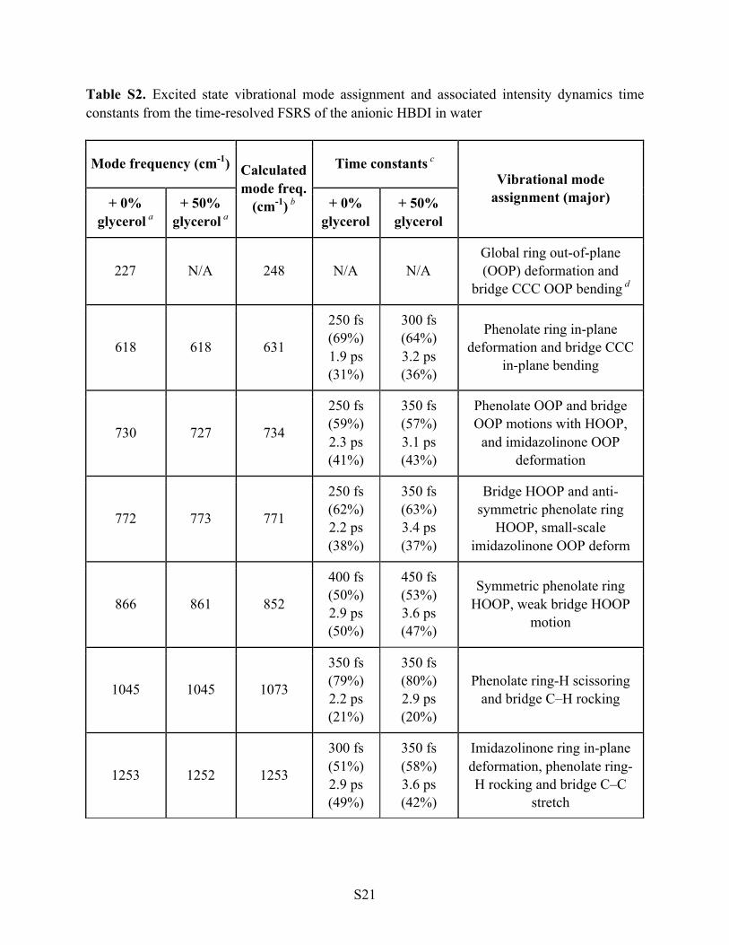
Table S2. Excited state vibrational mode assignment and associated intensity dynamics time constants from the time-resolved FSRS of the anionic HBDI in water

Mode frequency (cm-1) Calculated mode freq.

(cm-1) b

Time constants c Vibrational mode

assignment (major) + 0% glycerol a

+ 50% glycerol a

+ 0% glycerol

+ 50% glycerol

227 N/A 248 N/A N/A Global ring out-of-plane (OOP) deformation and

bridge CCC OOP bending d

618 618 631

250 fs (69%) 1.9 ps (31%)

300 fs (64%) 3.2 ps (36%)

Phenolate ring in-plane deformation and bridge CCC

in-plane bending

730 727 734

250 fs (59%) 2.3 ps (41%)

350 fs (57%) 3.1 ps (43%)

Phenolate OOP and bridge OOP motions with HOOP,

and imidazolinone OOP deformation

772 773 771

250 fs (62%) 2.2 ps (38%)

350 fs (63%) 3.4 ps (37%)

Bridge HOOP and anti-symmetric phenolate ring

HOOP, small-scale imidazolinone OOP deform

866 861 852

400 fs (50%) 2.9 ps (50%)

450 fs (53%) 3.6 ps (47%)

Symmetric phenolate ring HOOP, weak bridge HOOP

motion

1045 1045 1073

350 fs (79%) 2.2 ps (21%)

350 fs (80%) 2.9 ps (20%)

Phenolate ring-H scissoring and bridge C–H rocking

1253 1252 1253

300 fs (51%) 2.9 ps (49%)

350 fs (58%) 3.6 ps (42%)

Imidazolinone ring in-plane deformation, phenolate ring-H rocking and bridge C–C

stretch

S22

a The experimental Raman mode center frequency is obtained by least-squares fitting the ground-

state FSRS peaks of anionic HBDI in aqueous solution (pH=10) with 0% or 50% glycerol. Three

independent data sets on different days were used to obtain the average value and the precision is

within 1 cm-1. The Raman pump center wavelength was tuned to 550 nm.

b Singlet excited state (S1) vibrational frequencies of the geometrically optimized anionic HBDI

chromophore (see Figure 1b in main text for the chemical structure) are calculated using the

time-dependent DFT (TD-DFT) method with RB3LYP theory level and 6-311G+(d,p) basis sets

and –1 charge in Gaussian 09.27 The water solvent effect is incorporated using the integral

equation formalism variant polarizable continuum model (IEF-PCM) method. The normal mode

frequency scaling factor is 0.97 for the high-frequency modes (>1000 cm-1) and 1.01 for the low-

frequency modes (<1000 cm-1) as recommended to account for the frequency-dependent thermal

contributions to enthalpy and entropy.29 The observed Raman modes in Stokes FSRS (Figure 2a

and b, main text) is from the anionic HBDI chromophore in S1 after 400 nm photoexcitation.

c Typically, the integrated Raman peak intensities in Figure 2 can be least-squares fitted by two

exponentials that capture the essence of early-time structural dynamics of the chromophore.

Since the TA spectra reflect the population dynamics of HBDI, we use those time constants in

Table S1 as an initial guide for interpreting FSRS dynamics. However, some differences are

expected due to the separate tracking of electronic dynamics in TA whereas vibrational dynamics

in FSRS. The small increase of the second time constant upon adding 50% (v/v) glycerol is in

accord with the reported weak dependence of chromophore modes on medium viscosity.2,41

1572 1567 1561

200 fs (74%) 2.0 ps (26%)

240 fs (80%) 3.0 ps (20%)

Phenolate C=C and C=O stretch with bridge CC

stretch, imidazolinone C=O e and small-scale C=N stretch

S23

d This motion is consistent with the overall volume-conserving picture3,41 as nearby atoms move

in opposite directions out of the chromophore two-ring plane (Figure 4a).

e This assignment is corroborated by a transient IR spectroscopic study of the C=O vibration of

anionic HBDI in the S1 state,40 which did not observe the mode at a similar frequency region

above 1680 cm-1 for the neutral and cationic HBDI. The C=O mode likely downshifts its

frequency to mix with the aromatic ring vibrations as shown in the current mode assignment,

consistent with the mesomeric charge delocalization across the conjugated ring system of the

photoexcited anionic HBDI chromophore in solution. Notably, using the same level of theory

(DFT-RB3LYP) and basis sets (6-311G+(d,p)), this vibrational mode at the electronic ground

state (S0) has the frequency of 1647.3 cm-1 which after a frequency scaling of 0.985 yields ~1623

cm-1. The photoinduced mode frequency redshift due to electron redistribution from S0®S1 is

thus apparent from calculations (i.e., 1623®1561 cm-1).7,9,13

S24

Table S3. Frequency shift trend of three Raman marker bands and other key properties as a function of the chromophore ring twisting dihedral angle q

866 a 1253 a 1572 a Polarizability

(a.u.) Overall energy

(a.u.)

– 90 872 1258 1580 383.45 - 724.00102307

– 80 881 1256 1588 299.92 - 723.99511733

– 60 870 1255 1577 378.37 - 724.01302911

– 40 850 1264 1575 360.23 - 724.03522701

– 20 852 1270 1576 346.11 - 724.05250946

0 852 c 1272 c 1578 c 337.41 c - 724.06409524 c

20 851 1273 1577 339.45 - 724.06184931

40 852 1276 1576 344.58 - 724.05488068

60 853 1278 1576 353.66 - 724.04304504

80 856 1279 1580 366.30 - 724.02721848

90 857 1282 1579 373.44 - 724.01828613

a The experimentally observed excited state Raman mode frequencies that show charateristic

shifts in Figure 2a for the anionic HBDI in water (pH=10), also see Table 1 in main text. The

listed normal mode frequencies (unscaled) in this table are from DFT calculations of the

geometrically optimized deprotonated chromophore (–1 charge) at the RB3LYP level with 6-

31G+(d,p) basis sets and the IEFPCM solvent=water using Gaussian 09 software. To reduce

computational costs, the frequency shift trend (not the exact values) in S0 is used to gain insights

into the observed mode frequency shift in S1 along the particular dihedral twisting coordinate.

b This dihedral angle between the bridge C atom and the imidazolinone ring (depicted in Figure

1b) is fixed at discrete values from the positive to negative during DFT calculations to enable the

inspection of the chromophore ring-twisting-angle-dependent vibrational mode frequency shifts.

Dihedral angle q (°)

Mode freq. (cm-1) b

S25

c In comparison to these values calculated at q = 0° (angle fixed in this table, see Figure 1b for

depiction) which correspond to the optimized ground state structure of a nearly planar

chromophore in solution,4,41,42 the unscaled Raman mode frequency blue (red) shift, and the

overall energy and electric polarizability increase (decrease) are shown in blue (red) cells. The

observed vibrational frequency shifts better match the calculations in the positive q direction. To

further evaluate the robustness of this approach, we also performed the DFT-RB3LYP 6-

311G+(d,p) calculations. After geometrical optimization at the electroic ground state, the above-

mentioned dihedral angle is essentially zero (i.e., –0.004°) and the unscaled vibrational normal

mode frequencies are 854.4, 1276.3, and 1568.4 cm-1 with an overall energy of –724.21639540

a.u. The associated vibrational motions are mainly the phenolate ring symmetric HOOP, the

phenolate ring H-rock with bridge H-rock, and the phenolate C=C stretch with ring CC stretch

and some imidazolinone C=N stretch, respectively.

S26

ESI References

1 N. M. Webber, K. L. Litvinenko and S. R. Meech, J. Phys. Chem. B, 2001, 105, 8036-8039.

2 K. L. Litvinenko, N. M. Webber and S. R. Meech, J. Phys. Chem. A, 2003, 107, 2616-2623.

3 M. Vengris, I. H. M. van Stokkum, X. He, A. F. Bell, P. J. Tonge, R. van Grondelle and D. S.

Larsen, J. Phys. Chem. A, 2004, 108, 4587-4598.

4 R. Gepshtein, D. Huppert and N. Agmon, J. Phys. Chem. B, 2006, 110, 4434-4442.

5 K. Brejc, T. K. Sixma, P. A. Kitts, S. R. Kain, R. Y. Tsien, M. Ormö and S. J. Remington,

Proc. Natl. Acad. Sci. U. S. A., 1997, 94, 2306-2311.

6 A. D. Kummer, J. Wiehler, T. A. Schüttrigkeit, B. W. Berger, B. Steipe and M. E. Michel-

Beyerle, ChemBioChem, 2002, 3, 659-663.

7 C. Fang, R. R. Frontiera, R. Tran and R. A. Mathies, Nature, 2009, 462, 200-204.

8 B. G. Oscar, W. Liu, Y. Zhao, L. Tang, Y. Wang, R. E. Campbell and C. Fang, Proc. Natl.

Acad. Sci. U. S. A., 2014, 111, 10191-10196.

9 C. Fang, L. Tang, B. G. Oscar and C. Chen, J. Phys. Chem. Lett., 2018, 9, 3253–3263.

10 P. Kukura, D. W. McCamant and R. A. Mathies, Annu. Rev. Phys. Chem., 2007, 58, 461-488.

11 D. R. Dietze and R. A. Mathies, ChemPhysChem, 2016, 17, 1224–1251.

12 J.-M. L. Pecourt, J. Peon and B. Kohler, J. Am. Chem. Soc., 2001, 123, 10370-10378.

13 E. T. J. Nibbering, H. Fidder and E. Pines, Annu. Rev. Phys. Chem., 2005, 56, 337-367.

14 R. M. Hochstrasser, Proc. Natl. Acad. Sci. U. S. A., 2007, 104, 14190-14196.

15 W. Liu, Y. Wang, L. Tang, B. G. Oscar, L. Zhu and C. Fang, Chem. Sci., 2016, 7, 5484-5494.

16 Y.-X. Yan, E. B. Gamble and K. A. Nelson, J. Chem. Phys., 1985, 83, 5391-5399.

17 D. P. Hoffman and R. A. Mathies, Acc. Chem. Res., 2016, 49, 616-625.

S27

18 G. Batignani, G. Fumero, S. Mukamel and T. Scopigno, Phys. Chem. Chem. Phys., 2015, 17,

10454-10461.

19 B. G. Levine and T. J. Martínez, Annu. Rev. Phys. Chem., 2007, 58, 613-634.

20 J. P. Kraack, A. Wand, T. Buckup, M. Motzkus and S. Ruhman, Phys. Chem. Chem. Phys.,

2013, 15, 14487-14501.

21 G. D. Scholes, G. R. Fleming, L. X. Chen, A. Aspuru-Guzik, A. Buchleitner, D. F. Coker, G.

S. Engel, R. van Grondelle, A. Ishizaki, D. M. Jonas, J. S. Lundeen, J. K. McCusker, S.

Mukamel, J. P. Ogilvie, A. Olaya-Castro, M. A. Ratner, F. C. Spano, K. B. Whaley and X.

Zhu, Nature, 2017, 543, 647-656.

22 C. Chen, W. Liu, M. S. Baranov, N. S. Baleeva, I. V. Yampolsky, L. Zhu, Y. Wang, A.

Shamir, K. M. Solntsev and C. Fang, J. Phys. Chem. Lett., 2017, 8, 5921–5928.

23 C. Chen, M. S. Baranov, L. Zhu, N. S. Baleeva, A. Y. Smirnov, S. Zaitseva, I. V. Yampolsky,

K. M. Solntsev and C. Fang, Chem. Commun., 2019, 55, 2537-2540.

24 C. Chen, L. Zhu, M. S. Baranov, L. Tang, N. S. Baleeva, A. Y. Smirnov, I. V. Yampolsky, K.

M. Solntsev and C. Fang, J. Phys. Chem. B, 2019, DOI: 10.1021/acs.jpcb.1029b03201.

25 M. S. Baranov, K. A. Lukyanov, A. O. Borissova, J. Shamir, D. Kosenkov, L. V. Slipchenko,

L. M. Tolbert, I. V. Yampolsky and K. M. Solntsev, J. Am. Chem. Soc., 2012, 134, 6025-

6032.

26 S. S. Stavrov, K. M. Solntsev, L. M. Tolbert and D. Huppert, J. Am. Chem. Soc., 2006, 128,

1540-1546.

27 M. J. Frisch, G. W. Trucks, H. B. Schlegel, G. E. Scuseria, M. A. Robb, J. R. Cheeseman, G.

Scalmani, V. Barone, B. Mennucci, G. A. Petersson, H. Nakatsuji, M. Caricato, X. Li, H. P.

Hratchian, A. F. Izmaylov, J. Bloino, G. Zheng, J. L. Sonnenberg, M. Hada, M. Ehara, K.

S28

Toyota, R. Fukuda, J. Hasegawa, M. Ishida, T. Nakajima, Y. Honda, O. Kitao, H. Nakai, T.

Vreven, J. J. A. Montgomery, J. E. Peralta, F. Ogliaro, M. Bearpark, J. J. Heyd, E. Brothers,

K. N. Kudin, V. N. Staroverov, R. Kobayashi, J. Normand, K. Raghavachari, A. Rendell, J. C.

Burant, S. S. Iyengar, J. Tomasi, M. Cossi, N. Rega, J. M. Millam, M. Klene, J. E. Knox, J. B.

Cross, V. Bakken, C. Adamo, J. Jaramillo, R. Gomperts, R. E. Stratmann, O. Yazyev, A. J.

Austin, R. Cammi, C. Pomelli, J. W. Ochterski, R. L. Martin, K. Morokuma, V. G.

Zakrzewski, G. A. Voth, P. Salvador, J. J. Dannenberg, S. Dapprich, A. D. Daniels, Ö.

Farkas, J. B. Foresman, J. V. Ortiz, J. Cioslowski and D. J. Fox, Gaussian 09, Revision B.1,

Gaussian, Inc., Wallingford, CT, 2009.

28 A. P. Esposito, P. Schellenberg, W. W. Parson and P. J. Reid, J. Mol. Struct., 2001, 569, 25-

41.

29 J. P. Merrick, D. Moran and L. Radom, J. Phys. Chem. A, 2007, 111, 11683-11700.

30 M.-A. Elsliger, R. M. Wachter, G. T. Hanson, K. Kallio and S. J. Remington, Biochemistry,

1999, 38, 5296-5301.

31 A. F. Bell, X. He, R. M. Wachter and P. J. Tonge, Biochemistry, 2000, 39, 4423-4431.

32 S. P. Laptenok, J. Conyard, P. C. B. Page, Y. Chan, M. You, S. R. Jaffrey and S. R. Meech,

Chem. Sci., 2016, 7, 5747-5752.

33 G. Granucci, J. T. Hynes, P. Millie and T.-H. Tran-Thi, J. Am. Chem. Soc., 2000, 122,

12243-12253.

34 D. B. Spry, A. Goun and M. D. Fayer, J. Phys. Chem. A, 2007, 111, 230-237.

35 D. B. Spry and M. D. Fayer, J. Chem. Phys., 2008, 128, 084508.

36 Y. Wang, L. Tang, W. Liu, Y. Zhao, B. G. Oscar, R. E. Campbell and C. Fang, J. Phys.

Chem. B, 2015, 119, 2204-2218.

S29

37 T. Kumpulainen, B. Lang, A. Rosspeintner and E. Vauthey, Chem. Rev., 2017, 117, 10826-

10939.

38 J. L. McHale, Molecular Spectroscopy, Prentice-Hall, Upper Saddle River, NJ, 1999.

39 X. He, A. F. Bell and P. J. Tonge, FEBS Lett., 2003, 549, 35-38.

40 A. Usman, O. F. Mohammed, E. T. J. Nibbering, J. Dong, K. M. Solntsev and L. M. Tolbert,

J. Am. Chem. Soc., 2005, 127, 11214-11215.

41 D. Mandal, T. Tahara and S. R. Meech, J. Phys. Chem. B, 2004, 108, 1102-1108.

42 M. E. Martin, F. Negri and M. Olivucci, J. Am. Chem. Soc., 2004, 126, 5452-5464.