Quantum Chemistry for Solvated Molecules on Graphical ... · Quantum Chemistry for Solvated Molecules on Graphical Processing Units (GPUs) using Polarizable Continuum Models Fang

Liu, Luehr, Kulik, and Martínez – GPU-based PCM Calculations – Page 1

Quantum Chemistry for Solvated Molecules on Graphical Processing Units (GPUs) using Polarizable Continuum Models

Fang Liu,1,2 Nathan Luehr,1,2 Heather J. Kulik,1,3 Todd J. Martínez1,2

1Department of Chemistry and The PULSE Institute, Stanford University, Stanford, CA 94305 2SLAC National Accelerator Laboratory, Menlo Park, CA 94025

3Department of Chemical Engineering, Massachusetts Institute of Technology, Cambridge, MA 02139

Abstract: The conductor-like polarization model (C-PCM) with switching/Gaussian smooth dis-cretization is a widely used implicit solvation model in chemical simulations. However, its appli-cation in quantum mechanical calculations of large-scale biomolecular systems can be limited by computational expense of both the gas phase electronic structure and the solvation interaction. We have previously used graphical processing units (GPUs) to accelerate the first of these steps. Here, we extend the use of GPUs to accelerate electronic structure calculations including C-PCM solvation. Implementation on the GPU leads to significant acceleration of the generation of the required integrals for C-PCM. We further propose two strategies to improve the solution of the required linear equations: a dynamic convergence threshold and a randomized block-Jacobi pre-conditioner. These strategies are not specific to GPUs and are expected to be beneficial for both CPU and GPU implementations. We benchmark the performance of the new implementation us-ing over 20 small proteins in solvent environment. Using a single GPU, our method evaluates the C-PCM related integrals and their derivatives more than 10X faster than a conventional CPU-based implementation. Our improvements to the linear solver provide a further 3X acceleration. The overall calculations including C-PCM solvation require typically 20-40% more effort than their gas phase counterparts for moderate basis set and molecule surface discretization level. The relative cost of the C-PCM solvation correction decreases as the basis sets and/or cavity radii in-crease. Therefore description of solvation with this model should be routine. We also discuss ap-plications to the study of the conformational landscape of an amyloid fibril.


1. Introduction Modeling the influence of solvent in quantum chemical calculations is of great im-

portance to understanding solvation effects on electronic properties, nuclear distributions, spec-troscopic properties, acidity/basicity, and mechanisms of enzymatic and chemical reactions.1-4 Explicit inclusion of solvent molecules in quantum chemical calculations is computationally ex-pensive and requires extensive configurational sampling to determine equilibrium properties. Implicit models based on a dielectric continuum approximation are much more efficient, and are an attractive conceptual framework to describe solvent effects within a quantum mechanical (QM) approach.1

Among these implicit models, the apparent surface charge (ASC) methods are popular because they are easily implemented within QM algorithms and can provide excellent descrip-tions of the solvation of small- and medium-sized molecules when combined with empirical cor-rections for non-electrostatic solvation effects.4 ASC methods are based on the fact that the reac-tion potential generated by the presence of the solute charge distribution may be described in terms of an apparent charge distribution spread over the solute cavity surface. Methods such as the polarizable continuum models5 (PCM) and its variants such as conductor-like models (COSMO,6 C-PCM,7 also known as GCOSMO,8 and IEF-PCM9-11) are the most popular and ac-curate of these ASC algorithms.

While PCM calculations are much more efficient than their explicit solvent counterparts, their application in quantum mechanical calculations of large-scale biomolecular systems can be limited by CPU computational bottlenecks.4 Graphical processing units (GPUs), which are char-acterized as stream processors,12 are especially suitable for parallel computing involving massive data and numerous groups have explored their use for electronic structure theory.13-24 Implemen-tation of gas phase ab initio molecular calculations19-21 on GPUs led to greatly enhanced perfor-mance for large systems.25-26 Here, we harness the advances27 of stream processors to accelerate the computation of implicit solvent effects, effectively reducing the cost of PCM calculations. These improvements will enable simulations of large biomolecular systems in realistic environ-ments.

2. Conductor-like Polarizable Continuum Model The original Conductor-like screening model (COSMO) was introduced by Klamt and Schuurmann.6 In this approach, the molecule is embedded in a dielectric continuum with permit-tivity ε, and the solute forms a cavity within the dielectric with unit permittivity. In this electro-static model, the continuum is polarized by the solute, and the solute responds to the electric field of the polarized continuum. The electric field of the polarized continuum can be described by a set of surface polarization charges on the cavity surface. Then the electrostatic component of the solvation free energy can be represented by the interaction between the polarization charges and solute, in addition to the self-energy of the surface charges. For numerical convenience, the po-larization charge is often described by a discretization in terms of M finite charges residing on the cavity surface. The locations of the surface charges are fixed, and the values of the charges can be determined via a set of linear equations

Aq = − f (Bz + c) (1)


where q∈!M is the discretized surface charge distribution, A∈!M×M is the Coulomb interac-

tion between unit polarization charges on two cavity surface segments, B∈!M×N is the interac-tion between nuclei and a unit polarization charge on a surface segment, z ∈!N is the vector of nuclear charges for the N atoms in the solute molecule, and c∈!M is the interaction between the unit polarization charge on one surface segment and the total solute density. The parameter f=(ε-1)/(ε+k) is a correction factor for a polarizable continuum with finite dielectric constant. In the original COSMO paper, k was set to 0.5. Later work by Truong and Stefanovic8 (GCOSMO) and Cossi and Barone7 (C-PCM) suggested that k=0 was more appropriate on the basis of an analogy with Gauss’ Law. We use k=0 throughout in this work, although both cases are imple-mented in our code.

The precise form of the A, B, and c matrices/vectors depends on the specific techniques used in cavity discretization. In order to obtain continuous analytic gradients of solvation energy, York and Karplus28 proposed the Switching-Gaussian formalism (SWIG), where the cavity sur-face van der Waal spheres are discretized by Lebedev quadrature points. Polarization charges are represented as spherical Gaussians centered at each quadrature point (and not as simple point charges). Lange and Herbert29 proposed another form of switching function referred to here as “improved Switching-Gaussian” (ISWIG). Both SWIG and ISWIG formulations use the follow-ing definitions for the fundamental quantities A, B, and c:

Akl =

erf( ′ζ kl |!rk −!rl |)

| !rk −!rl |

(2)

Akk =

ζ k

2πSk

−1 (3)

BJk =

erf(ζ k |!rk −!RJ |)

| !rk −!RJ |

(4)

ck = PµνLµνk

µν∑ (5)

Lµνk = −(µ | Jk

screened |ν )

= − φµ!r( ) erf(ζ k |

!r − !rk |)| !r − !rk |

φν!r( )dr∫

(6)

where !rk is the location of the kth Lebedev point and

!RJ is the location of the Jth nucleus with

atomic radius RJ. The Gaussian exponent for the kth point charge is given as

ζ k =ζ

RI wk

(7)

where ζ is an optimized exponent for the specific Lebedev quadrature level being used (as tabu-lated28 by York and Karplus) and wk is the Lebedev quadrature weight for the kth point. The combined exponent is then given as:


ζ kl' = ζ kζ l

ζ k2 +ζ l

2 (8)

The atom-centered Gaussian basis functions used to describe the solute electronic wavefunction are denoted as φµ and φν and Pµν is the corresponding density matrix element. Finally, the switch-ing function which smoothes the boundary of the van der Waals spheres corresponding to each atom (and thus makes the solvation energy continuous) is given by Sk. For ISWIG, this switching function is expressed as:

Sk = Swf (!rk ,!RJ )

J ,k∉J

atoms

∏

Swf (!rk ,!RJ ) = 1−

12erf ζ k RJ −

!rk −!RJ( )⎡

⎣⎤⎦ + erf ζ k RJ +

!rk −!RJ( )⎡

⎣⎤⎦{ }

(9)

Similar, but more involved, definitions are used in SWIG (which we have also implemented, but only ISWIG will be used in this paper).

Once q is obtained by solving Eq. 1, the contribution of solvation effects to the Fock ma-trix is given by:

ΔFS = qk

k=1

M

∑ Lµνk (10)

where the Fock matrix of the solvated system is Fsolvated=F0+ΔFS and F0 is the usual gas phase Fock operator. This modified Fock matrix is then used for the self-consistent field (SCF) calcula-tion.

As usual, the atom-centered basis functions are contractions over a set of primitive atom-centered Gaussian functions:

φµ (r) = cµiχ i (r)

i=1

lµ

∑ (11)

Thus, the one electron integrals from Eq. 6 that are needed for the calculation of c and ΔFS are:

(µ | Jkscreened |ν ) =

j=1

lν

∑i=1

lµ

∑ cµicν j[χ i | Jkscreened | χ j ] (12)

where we use brackets to denote one-electron integrals over primitive basis functions and paren-theses to denote such integrals for contracted basis functions. In the following, we use the indices µ, ν for contracted basis functions and the indices i, j, k, l are used to refer to primitive Gaussian basis functions.

Smooth analytical gradients are available for COSMO SWIG/ISWIG calculations due to the use of a switching function which makes surface discretization points smoothly enter/exit the cavity definition. The total electrostatic solvation energy of COSMO is


ΔGels = (Bz)

†q+ c†q+ 12 fq†Aq (13)

Thus the PCM contribution to the solvated SCF energy gradient with respect to the nuclear coor-dinates RI of the Ith atom is given by

∇RI* (ΔGels ) = z

†(∇RIB†)q+ (∇RI

* c†)q+ 12 fq†(∇RI

A)q (14)

where ∇RI* denotes that the derivative with respect to the density matrix is not included. The con-

tribution of changes in the density matrix to the gradient is readily obtained from the gradient subroutine in vacuo (see supporting information for details).

In the COSMO-SCF process described above, there are three computationally intensive steps:

1. building c and ΔFS from Eqs. 5 and 10

2. solving the linear system in Eq. 1

3. evaluating the PCM gradients from Eq. 14

We discuss our acceleration strategies for each of these steps in Section 4 below.

3. Computational Methods We have implemented a GPU-accelerated COSMO formulation in a development version

of the TeraChem package. All COSMO calculations use parameters stated as follows unless oth-erwise specified. The environment dielectric constant corresponds to aqueous solvation (ε=78.39). The cavity uses an ISWIG29 discretization density of 110 points/atom and cavity radii which are 20% larger than the Bondi radii.30-32 An ISWIG screening threshold of 10-8 is used, meaning that molecular surface (MS) points with a switching function value less than this threshold are ignored. The conjugate gradient33 (CG) method is used to solve the PCM linear equations, with our newly proposed random Jacobi preconditioner (RBJ) with block size 100. The electrostatic potential matrix A is explicitly stored and used to calculate the necessary ma-trix-vector products during CG iterations.

In order to verify correctness and also to assess performance, we compare our code with the CPU based commercial package, Q-Chem34 4.2. For all the comparison test cases, Q-Chem uses exactly the same PCM settings as TeraChem, except for the CG preconditioner. Q-Chem uses the “diagonal decomposition” together with a block Jacobi preconditioner based on an octree spatial partition. We use OpenMP paralellization in Q-Chem because we found this to be faster than its MPI35 parallelized version based on our tests on these systems. In order to use OpenMP parallelization in this version of Q-Chem, we use the fast multipole method36-37 (FMM) and the “no matrix” mode, which rebuilds the A matrix “on the fly.”

We use a test set of six molecules (Figure 1) to investigate the relationship of the thresh-old and resulting error in the CG linear solve. For each molecule, we used five different struc-tures: one optimized structure, and four distorted structures obtained by performing classical mo-


lecular dynamics (MD) simulations on the first structure with Amber ff03 force fields38 at 500K. A summary of the name, size, and preparation method for these molecules, together with coordi-nate files, is provided in Supporting Information (SI).

In the performance section, we select a test set of 20 experimental protein structures iden-tified by Kulik, et al.39 where inclusion of a solvent environment was essential to find optimized structures in good agreement with experimental results. The molecules are listed in SI and range in size from around 100 to 500 atoms. Most were obtained from aqueous solution NMR experi-ments. For these test molecules, we conduct a number of restricted Hartree Fock (RHF) single point energy and nuclear gradient evaluations with the 6-31G basis set.40 These calculations are carried out in both PCM environment and in the gas phase. For some of these test molecules we also use basis sets of different sizes, including STO-3G,41 3-21G,42 6-31G*, 6-31G**,43 6-31++G,44 and 6-31+G*. We use these test molecules to identify optimum algorithm parameters and to study the performance of our approach as a function of basis set size.

In the application section, we investigate how COSMO solvation influences the confor-mational landscape of a model protein by expansive geometry optimization with both RHF and the range corrected exchange-correlation functional ωPBEh.45 Both of these approximations in-clude the full strength long-range exact exchange interactions that are vital to avoid self-interaction and delocalization errors. Such errors can lead to unrealistically small HOMO−LUMO gaps.46 We obtain seven different types of stationary point structures for the pro-tein in gas phase and in COSMO aqueous solution (ε=78.39), with a number of different basis sets (STO-3G, 3-21G, 6-31G). Grimme’s D3 dispersion correction47 is applied to some minimal basis set calculations, here referred to as RHF-D and ωPBEh-D.

4. Acceleration strategies 4a. Integral calculation on GPUs.

Building c and ΔFS requires calculation of one electron integrals and involves a signifi-cant amount of data parallelism, making these well suited for calculation on GPUs. The flowchart in Figure 2 summarizes our COSMO-SCF implementation. Following our gas phase SCF implementation,19,48 the COSMO related integrals needed for c and ΔFS are calculated in a direct SCF manner using GPUs. Here each GPU thread calculates integrals corresponding to one fixed primitive pair. However, the rest of the calculation, most significantly the solution of Eq. (1), is handled on the CPU.

From Eq. (5) and (10), it follows that the calculations for c and ΔFS are very similar, so one might be tempted to evaluate Lµν

k once and use it in both calculations. In practice this ap-proach is not efficient. Because ΔFS depends on the surface charge distribution (qk) and therefore on c through Eq. (1), c and ΔFS cannot be computed simultaneously. As the storage requirements for Lµν

k are excessive, it is ultimately more efficient to calculate the integrals for c and ΔFS sepa-rately from scratch.

The algorithm for evaluating ΔFS is shown schematically in Figure 3 for a system with three s shells and a GPU block size of 1×16 threads. The first and the third s shells contain 3 primitive Gaussian functions each; the second s shell has 2 primitive Gaussian functions. A


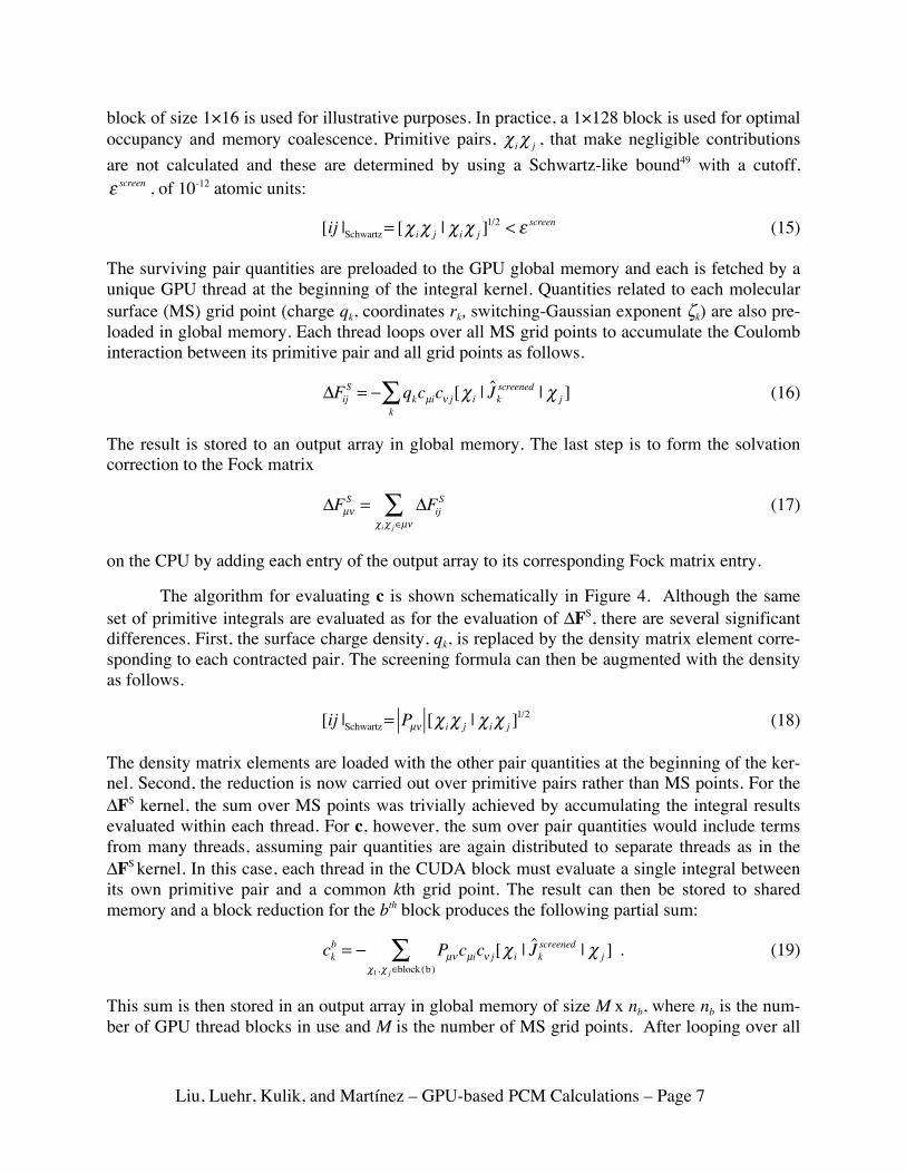
block of size 1×16 is used for illustrative purposes. In practice, a 1×128 block is used for optimal occupancy and memory coalescence. Primitive pairs, χ iχ j , that make negligible contributions are not calculated and these are determined by using a Schwartz-like bound49 with a cutoff, ε screen , of 10-12 atomic units:

[ij |Schwartz= [χ iχ j | χ iχ j ]1/2 < ε screen (15)

The surviving pair quantities are preloaded to the GPU global memory and each is fetched by a unique GPU thread at the beginning of the integral kernel. Quantities related to each molecular surface (MS) grid point (charge qk, coordinates rk, switching-Gaussian exponent ζk) are also pre-loaded in global memory. Each thread loops over all MS grid points to accumulate the Coulomb interaction between its primitive pair and all grid points as follows.

ΔFijS = − qk

k∑ cµicν j[χ i | Jk

screened | χ j ] (16)

The result is stored to an output array in global memory. The last step is to form the solvation correction to the Fock matrix

ΔFµνS = ΔFij

S

χiχ j∈µν∑ (17)

on the CPU by adding each entry of the output array to its corresponding Fock matrix entry.

The algorithm for evaluating c is shown schematically in Figure 4. Although the same set of primitive integrals are evaluated as for the evaluation of ΔFS, there are several significant differences. First, the surface charge density, qk, is replaced by the density matrix element corre-sponding to each contracted pair. The screening formula can then be augmented with the density as follows.

[ij |Schwartz= Pµν [χ iχ j | χ iχ j ]1/2 (18)

The density matrix elements are loaded with the other pair quantities at the beginning of the ker-nel. Second, the reduction is now carried out over primitive pairs rather than MS points. For the ΔFS kernel, the sum over MS points was trivially achieved by accumulating the integral results evaluated within each thread. For c, however, the sum over pair quantities would include terms from many threads, assuming pair quantities are again distributed to separate threads as in the ΔFS kernel. In this case, each thread in the CUDA block must evaluate a single integral between its own primitive pair and a common kth grid point. The result can then be stored to shared memory and a block reduction for the bth block produces the following partial sum:

ckb = − Pµνcµi

χ1,χ j∈block(b)∑ cν j[χ i | Jk

screened | χ j ] . (19)

This sum is then stored in an output array in global memory of size M x nb, where nb is the num-ber of GPU thread blocks in use and M is the number of MS grid points. After looping over all


MS grid points, the output array is copied to CPU, where we sum across different blocks and ob-

tain the final ck = ckb

b=1

nb

∑ .

Alternatively, the frequent block reductions can be eliminated from the kernel’s inner loop. Instead of mapping each primitive pair to a thread, each MS point is distributed to a sepa-rate thread. Each thread loops over primitive pairs to accumulate the Coulomb interaction be-tween its MS point and all primitive pairs, so that each entry of c is trivially accumulated within a single thread. This algorithm can be seen as a transpose of the ΔFS kernel and is referred to here as the “pair-driven kernel.” The reduction heavy algorithm is referred as the “MS-driven kernel.” Depending on the specifics of the hardware, one or the other of these might be optimal. We found little difference on the GPUs we used, and the results presented here use the MS-driven kernel.

All algorithms discussed above can be easily generalized to situations with angular mo-menta higher than s functions. In each loop, each thread calculates the Coulomb interaction be-tween a MS point and a batch of primitive pairs instead of a single primitive pair. For instance, for an sp integral, each GPU thread calculates integrals of 3 primitive pairs χ s ,χ p

x⎡⎣ ⎤⎦, χ s ,χ py⎡⎣ ⎤⎦, χ s ,χ p

z⎡⎣ ⎤⎦ in each loop. We wrote six separate GPU kernels for the following momentum classes: ss, sp, sd, pp, pd, dd. These kernels are launched sequentially.

4b. Conjugate Gradient Linear Solver The typical dimension of A in Eq. (1) is 103 ×103 or larger. Since Eq. (1) only needs to

be solved for a few right-hand sides, iterative methods can be applied and are much preferred over direct methods based on matrix inversion. Because the Coulomb operator is positive defi-nite, conjugate gradient (CG) methods are a good choice. At the k-th step of CG, we search for an approximate solution xk in the k-th Krylov subspace Kk (A,b) , and the distance between xk and the exact solution can be estimated by the residual vector:

rk = Axk − b (20)

The CG process terminates when the norm of the residual vector, ||rk||, falls below a threshold δ. A wise choice of δ can reduce the number of CG steps while maintaining accuracy.

The CG process converges more rapidly if A has small condition number, i.e. looks more like the identity. Preconditioning transforms one linear system to another that has the same solu-tion, but is easier to solve. One approach is to find a preconditioner matrix, C, that approximates A-1. Then, the problem CAx = Cb has the same solution as the original system but the matrix CA is better conditioned. The matrix A of Eq. (1) is often ill-conditioned because some of the diago-nal elements, which represent the self-energy of surface segments partially buried in the “switch-ing” area, are ~7-8 orders larger in magnitude than other diagonal elements.

In the following paragraphs we discuss our strategies to choose the CG convergence threshold δ and to generate a preconditioner for the linear equation Eq. (1).


4b-i) Dynamic convergence threshold for CG We must solve Eq. (1) in each SCF step. The traditional strategy (referred to here as the

fixed threshold scheme) is to choose a CG residual threshold value (e.g., δ≈10-6) and use this threshold for all SCF iterations. With this strategy, CG may require hundreds of iterations to converge in the first few SCF iterations for the computation of medium-sized systems (~500 at-oms), making the linear solve cost as much time as one Fock build. However, in the early SCF iterations, the solute electronic structure is still far from the final solution, so it is pointless to get an accurate solvent reaction field consistent with the inaccurate electronic structure. In other words, we can use larger δ for Eq. (1) in the early stages of the SCF, allowing us to reduce the number of CG iterations (and thus the total cost of the linear solves over the entire SCF process).

The simplest approach to leverage this observation uses a loose threshold δ1 for the early iterations of the SCF and switches to a tight threshold δ2 when close to SCF convergence. The maximum element of the DIIS error matrix XT(SPF-FPS)X, henceforth the “DIIS error,” was used as an indicator for SCF convergence, where S is the AO overlap matrix50 and X is the ca-nonical orthogonalization matrix. When the DIIS error reached 10-3, we switched from the loose threshold δ1 to the tight threshold δ2 in the CG solver. We define the loose and tight thresholds according to the relation δ1 = s ⋅δ 2 , where s >1 is a scaling factor. We call this adaptive strategy the “2-δ switching threshold.” Numerical experimentation on a variety of molecules showed that for reasonable values of δ2 (10-5-10-7), s=104 was a good choice which minimized the total num-ber of CG steps required for an SCF calculation. The effect of the 2-δ switching threshold strate-gy is shown in Figure 5. The number of CG steps in the first few SCF iterations is significantly reduced, and the total number of CG steps over the entire SCF procedure is halved. However, there is an abrupt increase of CG steps at the switching point, making that particular SCF itera-tion expensive. In order to remove this artifact and potentially increase the efficiency, we inves-tigated an alternative dynamic threshold strategy.

Luehr et al51 first proposed a dynamic threshold for the precision (32-bit single vs. 64-bit double) employed in evaluating two-electron integrals on GPUs. We extend this idea to the esti-mation of the appropriate CG convergence threshold for a given SCF energy error. We use a set of test molecules (shown in Figure 1) at both equilibrium and distorted nonequilibrium geome-tries (using RHF with different basis sets and ε=78.39) to empirically determine the relationship between the CG residual norm and the error it induces in the COSMO energy. We focus on the first COSMO iteration (i.e. the first formation of the solvated Fock matrix). The CG equations are first solved with a very accurate threshold for the CG residual norm, δ=10-10 atomic units. Then the CG equations are solved with progressively less accurate values of δ and the resulting error in the COSMO energy (compared to the calculation with δ=10-10) is tabulated. The average error for the six tested molecules is plotted as a function of the CG threshold in Figure 6. We found the resulting error to be insensitive to the basis set used. Therefore we used the 6-31G re-sults to generate an empirical equation relating the error and δ by a power-law fit. We further shifted this equation above twice the standard deviation to provide a bound for the error. This fit is plotted in Figure 6 and given by:

Err(δ ) = 0.01×δ 1.07 (21)


where Err(δ) is the COSMO energy error. We use Eq. (21) to dynamically adjust the CG thresh-old for the current SCF iteration by picking the value of that is predicted to result in a DIIS error safely below (10-3 times smaller than) the DIIS error of the previous SCF step. This error threshold ensures that error in CG convergence does not dominate the total SCF error. For the first SCF iteration, where there is no previous DIIS error as reference, we choose a loose thresh-old, δ=1. As shown in Figure 5, the number of CG steps required for each SCF iteration is now rather uniform. This strategy efficiently reduces CG steps without influencing the accuracy of the result. As shown in Figure 7, this approach typically provides a speed-up of 2X to 3X for sys-tems with 100-500 atoms.

4b-ii) Randomized block-Jacobi preconditioner for CG York and Karplus28 proposed a symmetric factorization, which is equivalent to Jacobi

preconditioning. Lange and Herbert52 later used a block Jacobi preconditioner, which accelerat-ed the calculation by about 20% for a large molecule. Their partitioning scheme (referred to as octree in our later discussion) of the matrix blocks is based on the spatial partition of MS points in the fast multipole method (FMM),36-37 implemented with an octree data structure. Here we propose a new randomized algorithm, which we refer to as RBJ, to efficiently generate the block diagonal preconditioner without detailed knowledge of the spatial distribution of surface charges. The primary advantage of the RBJ approach is that it is very simple to generate the precondition-er, although it may also have other benefits associated with randomized algorithms.53 As we will show, the performance of the RBJ preconditioner is at least as good as the more complicated oc-tree preconditioner.

Since A∈!m×m is symmetric, there exists some permutation matrix P such that the per-muted matrix is block-diagonal dominant. The block-diagonal matrix, M, is then con-structed from l × l diagonal blocks of PAP, and can be easily inverted to obtain as a preconditioner of A. We generate the permutation matrix in the following way: at the be-ginning of the CG solver, we randomly select a pivot Akk, sort the elements of the kth row by de-scending magnitude, pick the first column indices and form the first diagonal block of with the corresponding elements, repeating the procedure for the remaining indices until all rows of A have been accounted for. The inverse M-1 is then calculated and its non-zero entries (diagonal blocks) are stored and used throughout the Block Jacobi preconditioned CG algorithm.54

The efficiency of the RBJ preconditioner depends on the block size. As block size in-creases, more information about the original matrix A is kept in M, and the preconditioner C be-comes a better approximation to A-1. Thus, larger block sizes will lead to faster convergence of the CG procedure, at the cost of expending more effort to build C. In the limit where the block size is equal to the dimension of , C is an exact inverse of A and CG will converge in 1 step. However, in this case, building C is as computationally intensive as inverting A. We find that a block size of 100 is usually large enough to get significant reduction in the number of CG steps required for molecules with 100-500 atoms at a moderate discretization level 110 pts/atom (Fig-ures S1 and S2).

The performance of the randomized Block-Jacobi Preconditioner is shown in Figure 8, using as an example a single point COSMO RHF/6-31G calculation on a model protein (PDB ID: 2KJM, 516 atoms). Because RBJ is a randomized algorithm, each data point stands for the averaged results of 50 runs with different random seeds (error bars corresponding to the variance

δ

PAPC = PM−1P ≈ A−1

P

l M

A


are also shown). For this test case, RBJ with a block size of 100 reduces the total number of CG steps (matrix-vector products) by 40% compared to fixed threshold CG. Increasing the block size to 800 only slightly enhances the performance. As a reference, we also implemented the block Jacobi preconditioner based on the octree algorithm. In Figure 8, “octree-800” denotes the octree preconditioner with at most 800 points in each octree leaf box. Unlike RBJ, the number of points in each block of the octree is not fixed. For octree-800, the mean block size is 289. RBJ-100 al-ready outperforms octree-800 in the number of CG steps, despite the smaller size of blocks, be-cause RBJ provides better control of the block size and is less sensitive to the shape of the mo-lecular surface. For RBJ and octree preconditioners with the same average blocksize l , if the molecular shape is irregular (which is common for large asymmetric bio-molecules), the octree will contain both very small and large blocks for which l ≪ l or l ≫ l , respectively. This effect reduces the efficiency of the octree algorithm in two ways: 1) the small blocks tend to be poor at preconditioning and 2) the large blocks are less efficiently stored and inverted.

Another important aspect of the preconditioner is the overhead. For a system with a small number of MS points (e.g. less than 1000), the time saved by reducing CG steps cannot compen-sate the overhead of building blocks for RBJ. Thus, a standard Jacobi preconditioner is faster. For a system with a large number of MS points, the RBJ preconditioner is significantly faster than Jacobi, despite some overhead for building and inverting the blocks. As shown in Figure 7, compared with the “fixed +Jacobi” method, “fixed +RBJ” provides a 1.5X speedup, and “dynamic + RBJ” provides a 3X speedup.

4c. PCM gradient evaluation To efficiently evaluate Eq. (14), we note that ∇RI

A,∇RIB and ∇RI

c are all sparse and do not need to be calculated explicitly for all nuclear coordinates. This is a direct result of the fact that each MS point only moves with the atom on which it is centered, which is also true for the basis functions.

Therefore, the strategy here is to only evaluate the non-zero terms and add them to the corresponding gradients. Specifically, we focus on the evaluation of the second term ∇RI

* c†( )q in Eq. (14), which involves one-electron integrals and is the most demanding.

For each interaction between an MS point and a primitive pair, there are three non-zero derivatives: [∇RI

χ i | Jkscreened | χ j ],[χ i | Jk

screened |∇RJχ j ],[χ i |∇RK

Jkscreened | χ j ] , where χ i , χ j and MS

point k are located on atoms I, J and K, respectively. Therefore, (∇RI* c†)q is composed of three

parts

(∇RI* c†)q = ga[ij]

ij , i∈I∑ + gb[ij]

ij , j∈I∑ + gc[k]

k∈I∑

ga[ij]= Pµνcµicν j qk[∇ Iχ i | Jkscreened | χ j ]

k∑

gb[ij]= Pµνcµicν j qk[χ i | Jkscreened |∇Jχ j ]

k∑

gc[k]= qk Pµνcµicν j[χ i |∇K Jkscreened | χ j ]

ij∑

(22)

δ δδ


The calculation of ga and gb requires reduction over MS points, whereas gc requires reduction over primitive pairs. Therefore, the GPU algorithm for evaluation of (∇RI

* c†)q is a hybrid of the pair-driven ΔFS kernel and the MS-driven c kernel. Primitive pairs are prescreened with the den-sity-weighted Schwartz bound of Eq. (18). Each thread is assigned a single primitive pair, and loops over all MS points. Integrals ga[ij] and gb[ij] are accumulated within each thread. Finally, gc[k] is formed by a reduction sum within each block at the end of the kth loop, and the host CPU performs the cross-block reduction.

5. Performance A primary concern is the efficiency of a COSMO implementation compared with its gas

phase counterpart at the same level of ab initio theory. For our set of 20 proteins, Figure 9 shows the ratio of time consumed for COSMO compared to gas phase for RHF/6-31G single point en-ergy calculations. The COSMO calculations introduce at most 60% overhead. A similar ratio is achieved for the calculation of analytic gradients (Figure S3). Of course, this ratio will change with the level of quantum chemistry method and MS discretization. For a medium-sized mole-cule, the ratio decreases as the basis set size increases (Figure S4) because the COSMO-specific evaluations only involve one-electron integrals, whose computational cost grows more slowly than that of the gas phase Fock build. The COSMO overhead also decreases as larger cavity radii are used (Figure S5), because the number of MS points decreases with increasing cavity radii (more points are buried in the surface). This trend is expected to apply to molecules in a wide range of sizes (ca. 80-1500 atoms), as they share a general trend of decreasing the number of MS points with increasing radii (Figure S6). As a specific example, we turn to the Photoactive Yellow Protein (PYP, 1537 atoms). When the most popular choice55 of cavity radii (choosing atomic radii to be 20% larger than Bondi radii, i.e. 1.2*Bondi) is used (76577 MS points in total), the computational effort associated with COSMO takes approximately 25% of the total runtime for COSMO RHF/6-31G* single point calculation (Figure 10). When larger cavity radii (2.0*Bondi) are used (17266 MS points), the overhead for COSMO falls to 5% (Figure S7). Overall, our COSMO implementation typically requires about 20-40% more time than gas phase energy or gradient calculations, when a moderate basis set (6-31G) and typical cavity discretization level is used (radii=1.2*Bondi, 110 pts/atom). When a larger basis set or larger cavity radii is used, COSMO will cost less and be an even more insignificant part of the total computational cost relative to a gas phase calculation.

To demonstrate the advantage of a GPU-based implementation, we compare our perfor-mance to a commercially-available, CPU-based quantum chemistry code, Q-Chem.34 We take the smallest (PDB ID: 1Y49, 122 atoms) and the largest (PDB ID: 2KJM, 516 atoms) molecules in our test set of proteins and run a RHF/6-31G COSMO-ISWIG gradient calculation. TeraChem calculations were run on nVidia GTX TITAN GPUs and Intel Xeon [email protected] GHz CPUs. Q-Chem calculations were run on faster Intel Xeon [email protected] GHz CPUs. The number of GPUs/CPUs was varied in the tests to assess parallelization efficiency across multiple CPU/GPUs.

Timing results are summarized in Table 1 and Table 2. The PCM gradient calculation consists of four major parts: gas phase SCF (SCF steps in common with gas phase calculations), PCM SCF (including building the c vector, building ΔFS, and the CG linear solve), gas phase gradients, and PCM gradients. For each portion of the calculation, the runtime is annotated in


parenthesis with the percentage of the runtime for that step relative to total runtime. As explained above, Q-Chem uses OpenMP with no matrix mode and FMM. Comparisons with the MPI parallelized version of Q-Chem are provided in the supporting information. The MPI version of Q-Chem does not use FMM and stores the A matrix explicitly.

First we focus on the single CPU/GPU performance, and we compare the absolute runtime values. For both the small and large systems, the GPU implementation provides a 16X reduction in the total runtime relative to Q-Chem. This is in spite of the fact that Q-Chem is using a linear scaling FMM method. The speedup for different sections varies. The PCM gradient calculation has a speedup of over 40X, which is much higher than the overall speedup and the speedup for gas phase gradient. The FMM-based CG procedure in Q-Chem is slower than the version which explicitly stores the A matrix. Even compared to the latter, our CG implementation is about 3X faster (see SI). We attribute this to the preconditioning and dynamic threshold strategies described above. On the other hand, it is interesting to note that Q-Chem and TeraChem both spend a similar percentage(22-27%) of their time on PCM SCF and gradient evalutions, regardless of the difference in absolute runtime.

When we use multiple GPUs/CPUs, the total runtime decreases as a result of parallelization for both Q-Chem and TeraChem. However, for both programs, the percentage of time spent on PCM increases, showing that the parallel efficiency of the PCM related evaluations is lower than that of other parts of the calculation. Table 3 shows the parallel efficiency of TeraChem PCM calculation. The parallel efficiency is defined here as usual:56

efficiency = 1

PT1TP

(23)

where P is the number of GPUs/CPUs in use and T1/TP are the total runtime in serial/parallel, re-spectively. We compare the parallel efficiency of the four components of the PCM SCF calcula-tion: building c, building ΔFS, solving CG, and building the other terms in common with gas phase SCF. The parallel efficiencies of building c and ΔFS are both higher than that of gas phase SCF. However, for our CG implementation, the matrix-vector product is calculated on the CPU, which hampers the overall PCM SCF parallel efficiency. Similarly, parallel efficiency of the PCM gradient evaluation is limited by our serial computation of ∇A,∇B .

Overall, the GPU implementation of PCM calculations in TeraChem demonstrates significant speedups compared to Q-Chem, which serves as an example of the type of performance expected from a mature and efficient CPU-based COSMO implementation. However, our current implementations of CG and ∇A,∇B are conducted in serial on the CPU and do not benefit from parallelization. This is a direction for future improvement.

6. Applications As a representative application, we studied the structure of a protein fibril57 (protein se-

quence SSTVNG, PDB ID: 3FTR) with our COSMO code. This fibril is known to be able to form dimers called “steric zippers” that can pack and form amyloids -- insoluble fibrous protein aggregates. In each “zipper” pair, the two segments are tightly interdigitated β-sheets with no water molecules in the interface. The experimental structure of SSTVNG is a piece of the zipper from a fibril crystal. Kulik et al.39 found that minimal basis set ab initio, gas phase, geometry op-


timizations of a zwitterionic 3FTR monomer resulted in a structure with an unusual deprotona-tion of amide nitrogen atoms. In that structure, the majority of the amide protons are shared be-tween peptide bond nitrogen atoms and oxygen atoms, forming a covalent bond with the oxygen and a weaker hydrogen bond with the nitrogen. This phenomenon was explained as an artifact caused by both the absence of surrounding solvent and the minimal basis set. We were interested to quantify the degree to which these two approximations affected the outcome. Thus, we con-ducted more expansive geometry optimizations of 3FTR with and without COSMO to investi-gate how solvation influences the conformational landscape of the protein.

Stationary point structures of 3FTR were obtained as follows: starting from the two fea-tured structures found previously (an unusually protonated structure and a normally protonated stationary point structure close to experiment), geometry optimizations were conducted in gas phase and with COSMO to describe aqueous solvation (ε=78.39). Whenever a qualitatively dif-ferent structure was encountered, that structure was set as a new starting point for geometry op-timization under all levels of theory. Through this procedure, seven different types of stationary point structures were found (Figures 11 and 12 and Table S3) characterized by differing protona-tion states and backbone structures. We characterize the backbone structure by the end-to-end distance of the protein, computed as the distance between the Cα atoms of the first and last resi-due. We describe the protonation state of the amide N and O with a “protonation score,” defined as follows:

Protonation Score =dOi−Hi

i=1

nr

∑ / dNi−Hi

nr (24)

where nr is the number of residues; Oi, Hi, and Ni represent the amide O, H, N belonging to the ith residue (for the 1st residue, Hi represents the hydrogen atom at the N-terminus of the peptide closest to O). The higher the score is (e.g. > 1.5), the more closely hydrogens are bonded with amide nitrogens, indicating a correct protonation state.

The 3FTR crystal structure is zwitterionic with charged groups at both ends, and geome-try optimized structures of isolated 3FTR peptides will find minima that stabilize those charges. In the gas phase, the zwitterionic state’s energy is lowered during geometry minimizations in two ways. In one case, the C-terminus carboxylate is neutralized by a proximal amide H, resulting in unusually protonated local minima. In the other case, the energy is minimized by backbone fold-ing which brings the charged ends close to each other. Both rearrangements result in unexpected structures inconsistent with experiments in solution. We note however that such structural rear-rangements are known to occur in gas phase polypeptides.58

COSMO solvation largely corrects the protonation artifact observed in gas phase. Two types of severely unusually protonated (protonation score <1.5) local minima are observed. One (labeled min1u in Figures 11 and 12) has been previously reported with the straight backbone structure as crystal structure. The other unusually protonated local minimum is min2u, which has very similar protonation state as min1u, but a slightly bent backbone (backbone length <17Å). The normally protonated counterparts of min1u and min2u are min1n and min2n, which are the two minima most resembling the crystal structure. In gas phase calculations with 3-21G and 6-


31G, these four minima are all over 50 kcal/mol higher in energy than a folded structure (min4). COSMO solvation stabilizes min1n and min2n by about 50 kcal/mol, while leaving the anoma-lous min1u and min2u as high-energy structures (Table 4, Figure 11 and Figure 12). Moreover, this COSMO stabilization effect is already quite large for the smallest basis set (COSMO stabili-zation for different basis sets is summarized in Table 4). Although min1u and min2u are still pre-ferred over the normally protonated structures in both gas phase and COSMO STO-3G calcula-tions, this is perhaps expected since the basis set is so small.

COSMO also plays an important role in stabilizing an extended backbone structure. In gas phase calculations, the larger the end-to-end distance is, the less stable the structure tends to be. For both RHF/6-31G and ωPBEh calculations (Figure 11 and Figure 12, respectively), all unfolded structures (min1n, min1u, min2n, min2u, min2t) are very unstable in the gas phase with respect to the folded structure, min4. Among them, min1n and min2n have the largest charges separated by the largest distances (Table S6). COSMO stabilizes the terminal charges, thus sig-nificantly lowering the energy of min1 and min2. For COSMO RHF/6-31G, min2n is as stable as the folded min4. At the same time, the half folded and twisted structure, min3, is destabilized by COSMO.

For the most part, the local minima in the gas phase and solution are similar for this poly-peptide, even across a range of basis sets including minimal sets. However, the relative energies of these minima are strongly affected by solvation and basis set. Solvation is especially im-portant in this case because of the zwitterionic character of the polypeptide. This is expected on physical grounds (and the structures of gas phase polypeptides and proteins likely reflect this), and strongly suggests that solvation effects need to be modeled when using ab initio methods to describe protein structures.

7. Conclusions We have demonstrated that by implementing COSMO-related electronic integrals on

GPUs, dynamically adjusting the CG threshold for COSMO equations, and applying a new strat-egy for generating the block Jacobi preconditioner, we can significantly decrease the computa-tional effort required for COSMO calculations of large biomolecular systems. We achieve speedups compared to CPU-based codes of more than 15-60X. The computational overhead in-troduced by the COSMO calculation (relative to gas phase calculations) is quite small – typically 20-40%. Finally, we showed an example where COSMO solvation influences the geometry op-timization of proteins qualitatively. Our efficient implementation of COSMO will be useful for the study of protein structures.

Our approach for COSMO electron integral evaluation on GPU can be adapted for other variants of PCMs, such as the integral equation formalism (IEF-PCM or SS(V)PE).59 Since gen-eration of the randomized block Jacobi preconditioner only depends on the matrix itself (not the specific physical model used), the strategy can be applied to the preconditioning of CG in a vari-ety of fields. For instance, for linear scaling SCF, an alternative to diagonalization is the direct minimization of the energy functional60 with preconditioned CG. Another example is the solution of a large linear system with CG to obtain the perturbative correction to the wavefunction in CASPT2.61


In the future we will extend our acceleration strategies to non-equilibrium solvation, where the optical (electronic) dielectric constant is equilibrated with the solute while the orienta-tional dielectric constant is not.62-64 This will allow modeling of biomolecules in solution during photon absorption, fluorescence and phosphorescence processes. Our accelerated PCM code will also facilitate calculation of redox potential of metal complexes65 in solutes and pKa values for large biomolecules.66

8. Acknowledgments This work was supported by the AMOS program within the Chemical Sciences, Geosciences, and Biosciences Division of the Office of Basic Energy Sciences, Office of Science, US Depart-ment of Energy. TJM is grateful to the Department of Defense (Office of the Assistant Secretary of Defense for Research and Engineering) for a National Security Science and Engineering Fac-ulty Fellowship (NSSEFF).


Table 1. Timing data (seconds) for COSMO RHF/6-31G gradient calculation of TeraChem (TC) on GTX TITAN GPUs and Q-Chem (QC) on Intel Xeon CPUs ES-2643 @ 3.30 GHz.

molecule (#atoms,

#MS points)

#GPU /CPU core

Total runtime PCM gradient Gas phase gradient PCM SCF Gas Phase SCF

QC TC speed-up QC TC speed-up QC TC speed-up QC TC speed-up QC TC speed-up

1y49 (122,5922)

1 1877 116 16.2 88 (5%)

2 (2%) 39.4 410

(22%) 22

(19%) 18.5 502 (27%)

25 (22%) 19.9 878

(47%) 66

(57%) 13.3

4 705 40 17.5 85 (12%)

2 (4%) 56.8 84

(12%) 6

(15%) 14.1 337 (48%)

10 (25%) 33.5 200

(28%) 23

(57%) 8.7

8 581 31 18.9 89 (15%)

1 (4%) 67.2 72

(12%) 4

(12%) 20.2 309 (53%)

8 (27%) 36.8 111

(19%) 17

(57%) 6.3

2kjm (516,26025)

1 35345 1787 19.8 1960 (6%)

40 (2%) 48.9 6840

(19%) 417

(23%) 16.4 7789 (22%)

445 (25%) 17.5 18756

(53%) 885

(50%) 21.2

4 13506 623 21.7 2100 (16%)

26 (4%) 79.6 1415

(10%) 116

(19%) 12.2 6043 (45%)

181 (29%) 33.4 3948

(29%) 299

(48%) 13.2

8 11339 419 27.0 2088 (18%)

23 (6%) 89.2 1144

(10%) 59

(14%) 19.4 5768 (51%)

141 (33%) 41.1 2339

(21%) 196

(47%) 11.9

18

Table 2. As in Table 1, but detailed information for timing in the COSMO portion of the calculation.

molecule (#atoms,

#MS points)

#GPU/CPU

CG Build c Build ΔFs

QC TC speed-up QC TC speed-up QC TC speed-up

1y49 (122,5922)

1 221.3 (12%)

4.4 (4%) 39.8 149.5

(8%) 8.9

(8%) 16.8 131.0 (7%)

10.1 (9%) 13.0

4 55.5 (8%)

3.7 (9%) 15.4 149.6

(21%) 2.6

(7%) 56.7 131.5 (19%)

3.1 (8%) 42.4

8 28.0 (5%)

3.8 (12%) 7.5 149.6

(26%) 2.1

(7%) 70.9 131.6 (23%)

1.9 (6%) 70.6

2kjm (516,26025)

1 2335.1 (7%)

97.6 (5%) 18.8 2914.2

(8%) 130.9 (7%) 22.3 2539.3

(7%) 175.8 (10%) 14.4

4 581.9 (4%)

78.7 (13%) 7.2 2918.9

(22%) 38.5 (6%) 75.8 2541.7

(19%) 48.1 (8%) 52.8

8 310.8 (3%)

78.0 (19%) 3.8 2918.2

(26%) 20.2 (5%) 144.5 2538.7

(22%) 25.4 (6%) 100.1

19

Table 3. Parallel efficiency of TeraChem PCM calculation

#GPU PCM SCF Gas Phase SCF

PCM Gradient Gas phase Gradient CG Build c Build ΔFs Total 𝛁c Total

1y49 4 0.39 0.84 0.81 0.66 0.72 0.75 0.37 0.93 8 0.19 0.53 0.68 0.40 0.47 0.61 0.21 0.78

2kjm 4 0.39 0.85 0.91 0.64 0.74 0.85 0.38 0.90 8 0.19 0.81 0.87 0.43 0.56 0.79 0.21 0.88

20

Table 4. Energy difference (kcal/mol) between the normally and unusually protonated 3FTR minima.

Method/Basis Set Energy Difference (kcal/mol)

ΔE(min1u-min1n)a ΔE(min2u-min2n)b

COSMO Gas Phase COSMO Gas Phase RHF-D/-STO-3G -101 -178 -31 -77 RHF/STO-3G -106 -179 -27 -76 RHF/3-21G 77 13 83 6 RHF/6-31G 90 29 102 13

a min1n and min1u are minima with an extended backbone structure (as in the 3FTR crystal structure), where ‘n’ stands for normal protonation state, and ‘u’ stands for ‘unusual’ protonation state. b min2n and min2u are minima with slightly bent backbone structure.

21

Figure 1. Molecular geometries used to benchmark the correlation between COSMO energy error and CG convergence threshold.

(H2O)1339 Atoms (H2O)35

105 Atoms

(H2O)121 363 Atoms

3FTR 76 Atoms

2RMW 440 Atoms

1LVR 158 Atoms

(1

1LVRLL

22

Figure 2. Flowchart for COSMO SCF implementation

23

Figure 3. Algorithm for calculating ΔFS for ss integrals of a system compsed of 3 s shells (the first and the third s shells contain 3 primitive Gaussian function each. The second s shell has 2 primitive Gaussian functions). On top of the graph, the pale green array represents primitive pairs belonging to ss shell pairs. The GPU cores are represented by orange squares (threads) embedded in pale yellow rectangles (1 dimensional blocks with 16 threads/block). The output is an array where each entry stores a primitive pair integral. Primitive pair integrals are finally added to the Fock matrix entry of the conrresponding contracted function pair. All red lines and text indicate contracted Gaussian integrals. Blue arrows and text indicate memory operations.

24

Figure 4. MS point-driven algorithm for building for ss integrals of a system composed of 3 s shells (the first and the third s shells contain 3 primitive Gaussian functions each. The second s shell has 2 primitive Gaussian functions). The pale green array at the top of the figure represents primitive pairs belonging to ss shell pairs. The GPU cores are represented by orange squares (threads) embedded in pale yellow rectangles (1 dimensional blocks with 16 threads/block). The output is an array where each entry stores a primitive pair integral. Primitive pair integrals are finally added to the Fock matrix entry of the conrresponding contracted function pair. All red lines and text indicate contracted Gaussian integrals. Blue arrows and text indicate memory operations.

c

25

Figure 5. Number of CG steps taken in each SCF iteration for different CG residual convergence threshold schemes in COSMO RHF/6-31G calculation on a model protein (PDB ID: 2KJM, 516 atoms, shown in inset).

26

Figure 6. Average absolute error in first COSMO energies versus the CG residual convergence threshold. Both minimized and distored nonequilibrium geometries for the the test set are included in averages. Error bars represent two standard deviations above the mean. The black line represents the empirical error bound given by Eq. (21).

27

Figure 7. Speed up for CG linear solve methods compared to fixed δ + Jacobi preconditioner of TeraChem for COSMO RHF/6-31G single point energy calculations. Calculations were carried out on 1 GPU (GeForce GTX TITAN).

28

Figure 8. Number of CG steps taken in each SCF iteration for different choices of CG preconditioner in COSMO RHF/6-31G calculation on a model protein (PDB ID: 2KJM, 516 atoms, shown in inset). RBJ-100 and RBJ-800 represent the randomized block Jacobi preconditioner with block size of 100 and 800, respectively. The block Jacobi preconditioner based on an octree partition of surface points (denoted octree-800) is also shown, where the maximum number of points in a box is 800.

29

Figure 9. Ratio of time for COSMO versus gas phase single point energy calculation for 20 small pro-teins at RHF/6-31G level. Dynamic precision for 2-electron integrals is used with COSMO cavity radii chosen as 1.2*Bondi radii. An ISWIG discretization scheme is used with 110 Lebedev points/atom.

30

Figure 10. Breakdown of timings by SCF iteration for components of COSMO RHF/6-31G* calculation on Photoactive Yellow Protein (PYP) with cavity radii chosen as Bondi radii scaled by 1.2.

31

Figure 11. Different minima (min1n, min1u, min2n, min2u, min3, min4) of 3FTR found with RHF/6-31G geometry optimizations in COSMO and in the gas phase. The x-axis is the collective variable that characterizes the backbone folding. The y-axis is the total energy including solvation energy of the geometries. Each optimized structure is represented by a symbol in the graph and labeled by name with the backbone structure (C, O, N and H are colored grey, red, blue and white). Sidechains are omitted for clarity.

32

Figure 12. As in Figure 11, but using ωPBEh/6-31G.

33

References 1. Tomasi, J.; Mennucci, B.; Cammi, R., Quantum Mechanical Continuum Solvation Models. Chem. Rev. 2005, 105 (8), 2999-3094. 2. Tomasi, J.; Persico, M., Molecular Interactions in Solution: An Overview of Methods Based on Continuous Distributions of the Solvent. Chem. Rev. 1994, 94 (7), 2027-2094. 3. Cramer, C. J.; Truhlar, D. G., Implicit Solvation Models:   Equilibria, Structure, Spectra, and Dynamics. Chem. Rev. 1999, 99 (8), 2161-2200. 4. Orozco, M.; Luque, F. J., Theoretical Methods for the Description of the Solvent Effect in Biomolecular Systems. Chem. Rev. 2000, 100 (11), 4187-4226. 5. Miertuš, S.; Scrocco, E.; Tomasi, J., Electrostatic interaction of a solute with a continuum. A direct utilizaion of AB initio molecular potentials for the prevision of solvent effects. Chem. Phys. 1981, 55 (1), 117-129. 6. Klamt, A.; Schuurmann, G., COSMO: a new approach to dielectric screening in solvents with explicit expressions for the screening energy and its gradient. J. Chem. Soc. Perkins. Trans. 2 1993, (5), 799-805. 7. Barone, V.; Cossi, M., Quantum Calculation of Molecular Energies and Energy Gradients in Solution by a Conductor Solvent Model. J. Phys. Chem. A 1998, 102 (11), 1995-2001. 8. Truong, T. N.; Stefanovich, E. V., A new method for incorporating solvent effect into the classical, ab initio molecular orbital and density functional theory frameworks for arbitrary shape cavity. Chem. Phys. Lett. 1995, 240 (4), 253-260. 9. Mennucci, B.; Cancès, E.; Tomasi, J., Evaluation of Solvent Effects in Isotropic and Anisotropic Dielectrics and in Ionic Solutions with a Unified Integral Equation Method:   Theoretical Bases, Computational Implementation, and Numerical Applications. J. Phys. Chem. B 1997, 101 (49), 10506-10517. 10. Cancès, E.; Mennucci, B.; Tomasi, J., A new integral equation formalism for the polarizable continuum model: Theoretical background and applications to isotropic and anisotropic dielectrics. J. Chem. Phys. 1997, 107 (8), 3032-3041. 11. Tomasi, J.; Mennucci, B.; Cancès, E., The IEF version of the PCM solvation method: an overview of a new method addressed to study molecular solutes at the QM ab initio level. Journal of Molecular Structure: THEOCHEM 1999, 464 (1–3), 211-226. 12. Kapasi, U. J.; Rixner, S.; Dally, W. J.; Khailany, B.; Ahn, J. H.; Mattson, P.; Owens, J. D., Programmable Stream Processors. Computer 2003, 36 (8), 54-62. 13. Asadchev, A.; Allada, V.; Felder, J.; Bode, B. M.; Gordon, M. S.; Windus, T. L., Uncontracted Rys Quadrature Implementation of up to G Functions on Graphical Processing Units. J. Chem. Theo. Comp. 2010, 6, 696-704. 14. Asadchev, A.; Gordon, M. S., New Multithreaded Hybrid CPU/GPU Approach to Hartree-Fock. J. Chem. Theo. Comp. 2012, 8, 4166-4176. 15. Vogt, L.; Olivares-Amaya, R.; Kermes, S.; Shao, Y.; Amador-Bedolla, C.; Aspuru-Guzik, A., Accelerating Resolution-of-the-Identity Second-Order Moller-Plesset Quantum Chemistry Calculations with Graphical Processing Units. J. Phys. Chem. A 2008, 112, 2049-2057. 16. Andrade, X.; Aspuru-Guzik, A., Real-space Density Functional Theory on Graphical Processing Units: Computational Approach and Comparison to Gaussian Basis Set Methods. J. Chem. Theo. Comp. 2013, 9, 4360-4373. 17. Yasuda, K., Two-electron integral evaluation on the graphics processor unit. J. Comp. Chem. 2008, 29, 334-342. 18. DePrince, A. E.; Hammond, J. R., Coupled Cluster Theory on Graphical Processing Units. I. The Coupled Cluster Doubles Method. J. Chem. Theo. Comp. 2011, 7, 1287-1295.

34

19. Ufimtsev, I. S.; Martinez, T. J., Quantum Chemistry on Graphical Processing Units. 2. Direct Self-Consistent-Field Implementation. J. Chem. Theo. Comp. 2009, 5 (4), 1004-1015. 20. Ufimtsev, I. S.; Martinez, T. J., Quantum Chemistry on Graphical Processing Units. 3. Analytical Energy Gradients, Geometry Optimization, and First Principles Molecular Dynamics. J. Chem. Theo. Comp. 2009, 5 (10), 2619-2628. 21. Ufimtsev, I. S.; Martínez, T. J., Quantum Chemistry on Graphical Processing Units. 1. Strategies for Two-Electron Integral Evaluation. J. Chem. Theo. Comp. 2008, 4 (2), 222-231. 22. Ufimtsev, I. S.; Martinez, T. J., Graphical Processing Units for Quantum Chemistry. Comp. in Sci. Eng. 2008, 10, 26-34. 23. Miao, Y.; Merz, K. M., Acceleration of Electron Repulsion Integral Evaluation on Graphics Processing Units via Use of Recurrence Relations. J. Chem. Theo. Comp. 2013, 9, 965-976. 24. Kussmann, J.; Ochsenfeld, C., Preselective screening for linear-scaling exact exchange-gradient calculations for graphics processing units and strong-scaling massively parallel calculations. J. Chem. Theo. Comp. 2015, 11, 918-922. 25. Ufimtsev, I. S.; Luehr, N.; Martinez, T. J., Charge Transfer and Polarization in Solvated Proteins from Ab Initio Molecular Dynamics. J. Phys. Chem. Lett. 2011, 2 (14), 1789-1793. 26. Isborn, C. M.; Luehr, N.; Ufimtsev, I. S.; Marti nez, T. J., Excited-State Electronic Structure with Configuration Interaction Singles and Tamm–Dancoff Time-Dependent Density Functional Theory on Graphical Processing Units. J. Chem. Theo. Comp. 2011, 7 (6), 1814-1823. 27. http://www.petachem.com/. 28. York, D. M.; Karplus, M., A Smooth Solvation Potential Based on the Conductor-Like Screening Model. J. Phys. Chem. A 1999, 103 (50), 11060-11079. 29. Lange, A. W.; Herbert, J. M., A smooth, nonsingular, and faithful discretization scheme for polarizable continuum models: The switching/Gaussian approach. J. Chem. Phys. 2010, 133 (24), 244111. 30. Bondi, A., Van Der Waals Volumes + Radii. J. Phys. Chem. 1964, 68 (3), 441-&. 31. Rowland, R. S.; Taylor, R., Intermolecular nonbonded contact distances in organic crystal structures: Comparison with distances expected from van der Waals radii. J. Phys. Chem. 1996, 100 (18), 7384-7391. 32. Mantina, M.; Chamberlin, A. C.; Valero, R.; Cramer, C. J.; Truhlar, D. G., Consistent van der Waals Radii for the Whole Main Group. J. Phys. Chem. A 2009, 113 (19), 5806-5812. 33. Golub, G. H.; Van Loan, C. F., Matrix computations. 4th ed. ed.; Johns Hopkins University Press: Baltimore, 2013. 34. Shao, Y.; Molnar, L. F.; Jung, Y.; Kussmann, J.; Ochsenfeld, C.; Brown, S. T.; Gilbert, A. T. B.; Slipchenko, L. V.; Levchenko, S. V.; O'Neill, D. P.; DiStasio Jr, R. A.; Lochan, R. C.; Wang, T.; Beran, G. J. O.; Besley, N. A.; Herbert, J. M.; Yeh Lin, C.; Van Voorhis, T.; Hung Chien, S.; Sodt, A.; Steele, R. P.; Rassolov, V. A.; Maslen, P. E.; Korambath, P. P.; Adamson, R. D.; Austin, B.; Baker, J.; Byrd, E. F. C.; Dachsel, H.; Doerksen, R. J.; Dreuw, A.; Dunietz, B. D.; Dutoi, A. D.; Furlani, T. R.; Gwaltney, S. R.; Heyden, A.; Hirata, S.; Hsu, C.-P.; Kedziora, G.; Khalliulin, R. Z.; Klunzinger, P.; Lee, A. M.; Lee, M. S.; Liang, W.; Lotan, I.; Nair, N.; Peters, B.; Proynov, E. I.; Pieniazek, P. A.; Min Rhee, Y.; Ritchie, J.; Rosta, E.; David Sherrill, C.; Simmonett, A. C.; Subotnik, J. E.; Lee Woodcock Iii, H.; Zhang, W.; Bell, A. T.; Chakraborty, A. K.; Chipman, D. M.; Keil, F. J.; Warshel, A.; Hehre, W. J.; Schaefer Iii, H. F.; Kong, J.; Krylov, A. I.; Gill, P. M. W.; Head-Gordon, M., Advances in methods and algorithms in a modern quantum chemistry program package. Phys. Chem. Chem. Phys. 2006, 8 (27), 3172-3191. 35. Gabriel, E.; Fagg, G. E.; Bosilca, G.; Angskun, T.; Dongarra, J. J.; Squyres, J. M.; Sahay, V.; Kambadur, P.; Barrett, B.; Lumsdaine, A.; Castain, R. H.; Daniel, D. J.; Graham, R. L.; Woodall, T. S., Open MPI: Goals, concept, and design of a next generation MPI implementation. Lect Notes Comput Sc 2004, 3241, 97-104.

35

36. Greengard, L.; Rokhlin, V., A Fast Algorithm for Particle Simulations. J. Comp. Phys. 1987, 73 (2), 325-348. 37. Li, P.; Johnston, H.; Krasny, R., A Cartesian treecode for screened coulomb interactions. J. Comp. Phys. 2009, 228 (10), 3858-3868. 38. Case, D. e.; Darden, T.; Cheatham, T.; Simmerling, C.; Wang, J.; Duke, R.; Luo, R.; Walker, R.; Zhang, W.; Merz, K. Amber 11; University of California: 2010. 39. Kulik, H. J.; Luehr, N.; Ufimtsev, I. S.; Martinez, T. J., Ab Initio Quantum Chemistry for Protein Structures. J. Phys. Chem. B 2012, 116 (41), 12501-12509. 40. Ditchfie.R; Hehre, W. J.; Pople, J. A., Self-Consistent Molecular-Orbital Methods .9. Extended Gaussian-Type Basis for Molecular-Orbital Studies of Organic Molecules. J. Chem. Phys. 1971, 54 (2), 724-&. 41. Hehre, W. J.; Stewart, R. F.; Pople, J. A., Self-Consistent Molecular-Orbital Methods .I. Use of Gaussian Expansions of Slater-Type Atomic Orbitals. J. Chem. Phys. 1969, 51 (6), 2657-&. 42. Binkley, J. S.; Pople, J. A.; Hehre, W. J., Self-Consistent Molecular-Orbital Methods .21. Small Split-Valence Basis-Sets for 1st-Row Elements. J Am Chem Soc 1980, 102 (3), 939-947. 43. Harihara.Pc; Pople, J. A., Influence of Polarization Functions on Molecular-Orbital Hydrogenation Energies. Theo. Chim. Acta 1973, 28 (3), 213-222. 44. Frisch, M. J.; Pople, J. A.; Binkley, J. S., Self-Consistent Molecular-Orbital Methods .25. Supplementary Functions for Gaussian-Basis Sets. J. Chem. Phys. 1984, 80 (7), 3265-3269. 45. Rohrdanz, M. A.; Martins, K. M.; Herbert, J. M., A long-range-corrected density functional that performs well for both ground-state properties and time-dependent density functional theory excitation energies, including charge-transfer excited states. J. Chem. Phys. 2009, 130 (5), -. 46. Stein, T.; Eisenberg, H.; Kronik, L.; Baer, R., Fundamental Gaps in Finite Systems from Eigenvalues of a Generalized Kohn-Sham Method. Physical Review Letters 2010, 105 (26), 266802. 47. Grimme, S.; Antony, J.; Ehrlich, S.; Krieg, H., A consistent and accurate ab initio parametrization of density functional dispersion correction (DFT-D) for the 94 elements H-Pu. J. Chem. Phys. 2010, 132 (15), -. 48. Almlof, J.; Faegri, K.; Korsell, K., Principles for a Direct Scf Approach to Lcao-Mo Abinitio Calculations. J. Comp. Chem. 1982, 3 (3), 385-399. 49. Whitten, J. L., Coulombic potential energy integrals and approximations. J. Chem. Phys. 1973, 58 (10), 4496-4501. 50. Pulay, P., Improved Scf Convergence Acceleration. J. Comp. Chem. 1982, 3 (4), 556-560. 51. Luehr, N.; Ufimtsev, I. S.; Martinez, T. J., Dynamic Precision for Electron Repulsion Integral Evaluation on Graphical Processing Units (GPUs). J. Chem. Theo. Comp. 2011, 7 (4), 949-954. 52. Lange, A. W.; Herbert, J. M., The polarizable continuum model for molecular electrostatics: Basic theory, recent advances, and future challenges. In Many-Body Effects and Electrostatics in Multi-Scale Computations of Biomolecules, Q. Cui, P. R., and M. Meuwly, Ed. 2014. 53. Liberty, E.; Woolfe, F.; Martinsson, P.-G.; Rokhlin, V.; Tygert, M., Randomized algorithms for the low-rank approximation of matrices. Proc. Natl. Acad. Sci. 2007, 104, 20167-20172. 54. Hegland, M.; Saylor, P. E., Block jacobi preconditioning of the conjugate gradient method on a vector processor. International Journal of Computer Mathematics 1992, 44 (1-4), 71-89. 55. Amovilli, C.; Barone, V.; Cammi, R.; Cancès, E.; Cossi, M.; Mennucci, B.; Pomelli, C. S.; Tomasi, J., Recent Advances in the Description of Solvent Effects with the Polarizable Continuum Model. In Advances in Quantum Chemistry, Per-Olov, L., Ed. Academic Press: 1998; Vol. Volume 32, pp 227-261. 56. Kumar, V., Introduction to parallel computing : design and analysis of algorithms. Benjamin/Cummings Pub. Co.: Redwood City, Calif., 1994; p xv, 597 p. 57. Wiltzius, J. J.; Landau, M.; Nelson, R.; Sawaya, M. R.; Apostol, M. I.; Goldschmidt, L.; Soriaga, A. B.; Cascio, D.; Rajashankar, K.; Eisenberg, D., Molecular mechanisms for protein-encoded inheritance. Nat. Struct. Mol. Bio. 2009, 16, 973-979.

36

58. Marchese, R.; Grandori, R.; Carloni, P.; Raugei, S., On the Zwitterionic Nature of Gas-Phase Peptides and Protein Ions. PLOS Comp. Bio. 2010, 6, e1000775. 59. Chipman, D. M., Reaction field treatment of charge penetration. J. Chem. Phys. 2000, 112 (13), 5558-5565. 60. Millam, J. M.; Scuseria, G. E., Linear scaling conjugate gradient density matrix search as an alternative to diagonalization for first principles electronic structure calculations. J. Chem. Phys. 1997, 106 (13), 5569-5577. 61. Karlström, G.; Lindh, R.; Malmqvist, P.-Å.; Roos, B. O.; Ryde, U.; Veryazov, V.; Widmark, P.-O.; Cossi, M.; Schimmelpfennig, B.; Neogrady, P.; Seijo, L., MOLCAS: a program package for computational chemistry. Computational Materials Science 2003, 28 (2), 222-239. 62. Klamt, A., Calculation of UV/Vis Spectra in Solution. J. Phys. Chem. 1996, 100 (9), 3349-3353. 63. Cammi, R.; Corni, S.; Mennucci, B.; Tomasi, J., Electronic excitation energies of molecules in solution: State specific and linear response methods for nonequilibrium continuum solvation models. J. Chem. Phys. 2005, 122 (10), -. 64. Cossi, M.; Barone, V., Separation between Fast and Slow Polarizations in Continuum Solvation Models. J. Phys. Chem. A 2000, 104 (46), 10614-10622. 65. Wang, L.-P.; Van Voorhis, T., A Polarizable QM/MM Explicit Solvent Model for Computational Electrochemistry in Water. J. Chem. Theo. Comp. 2012, 8 (2), 610-617. 66. Li, H.; Robertson, A. D.; Jensen, J. H., Very fast empirical prediction and rationalization of protein pKa values. Proteins 2005, 61 (4), 704-721.

Documents

Quantum Chemistry for Solvated Molecules on Graphical ... · Quantum Chemistry for Solvated Molecules on Graphical Processing Units (GPUs) using Polarizable Continuum Models Fang