Deep Cyclonic Circulation in the Gulf of Mexicosturges/Pubs/DeHaan_SturgesJPO_2005.pdf · from observations, we do not know the deep flow well. Several numerical models include the

Deep Cyclonic Circulation in the Gulf of Mexico

CHRISTOPHER J. DEHAAN AND WILTON STURGES

Department of Oceanography, The Florida State University, Tallahassee, Florida

(Manuscript received 20 December 2002, in final form 10 March 2005)

ABSTRACT

The anticyclonic Loop Current dominates the upper-layer flow in the eastern Gulf of Mexico, with aweaker mean anticyclonic pattern in the western gulf. There are reasons, however, to suspect that the deepmean flow should actually be cyclonic. Topographic wave rectification and vortex stretching contribute tothis cyclonic tendency, as will the supply of cold incoming deep water at the edges of the basin. The authorsfind that the deep mean flow is cyclonic both in the eastern and western gulf, with speeds on the order of1–2 cm s�1 at 2000 m. Historical current-meter mooring data, as well as profiling autonomous Lagrangiancirculation explorer (PALACE) floats (at 900 m), suggest that vertical geostrophic shear relative to 1000 mgives a surprisingly accurate result in the interior of the basin. The temperature around the edges of thebasin at 2000 m is coldest near the Yucatan Channel, where Caribbean Sea water is colder by �0.1°C. Thetemperature increases steadily with distance in the counterclockwise direction from the Yucatan, consistentwith a deep mean cyclonic boundary flow.

1. Introduction

The Loop Current and the warm-core rings that de-tach from it dominate the upper-layer flow in the Gulfof Mexico. The well-known primary flow enters theCaribbean Sea from the open Atlantic Ocean, flowsinto the Gulf of Mexico through the Yucatan Channel,the constriction between Mexico and Cuba, and thenleaves the gulf to form the Florida Current and GulfStream (see, e.g., Johns et al. 2002; Schmitz and Rich-ardson 1991; Niiler and Richardson 1973). There havebeen several attempts to summarize the flow in the gulfusing the historical data (see Hoffmann and Worley1986; Molinari et al. 1978). The upper-layer flow hasbeen observed fairly well in recent years by satelliteobservations of temperature and sea-surface height.The main flow is restricted to approximately 850 mbecause the Loop Current exits through the Straits ofFlorida.

The deep flow has been described by Hamilton(1990). A magnificent new set of mooring data in theYucatan Channel has been reported recently (Bunge etal. 2002; Ochoa et al. 2001; Sheinbaum et al. 2002).

The mean upper-layer flow is well described by al-most any temperature or density surface above themain thermocline. Figure 1 shows the mean tempera-ture at 400 m. The mean depth of the 27.0 �� densitysurface shows a similar structure. The dots that appearto be data points are local means at essentially randomconcentrations of �5–10 hydrostations; these were se-lected, using data from many years, from the full his-torical National Oceanographic Data Center (NODC)database (Conkright et al. 2000) in an attempt to sup-press the very great time variability of warm-core ringspropagating to the west.

Two individual warm-core features are evident inFig. 1. In the east, although the Loop Current positionis quite variable, a clear mean emerges. In the centraland western gulf the anticyclonic pattern is maintainedboth by the mean wind field and by the passage of largewarm-core rings that have separated from the LoopCurrent. The relative importance of these two forcingmechanisms remains an open question.

Though we know the upper-layer flow fairly wellfrom observations, we do not know the deep flow well.Several numerical models include the Gulf of Mexico,but good observations at depth are scarce. The intrigu-ing fact, however, is that the temperature signature ofthe upper-layer flow, so obviously anticyclonic, appearsto extend to depths of �1500 to 2000 m in the data.Because we know that the flow in the Florida Current

Corresponding author address: Christopher DeHaan, NavalOceanographic Office, Code N33, Models Division, 1002 BalchBlvd., Stennis Space Center, MS 39522.E-mail: [email protected]

OCTOBER 2005 D E H A A N A N D S T U R G E S 1801

© 2005 American Meteorological Society

JPO2790

penetrates only to �850 m, we might expect the warm-core structure of Fig. 1 to extend only to that depth—whereas, in fact, it goes much deeper.

Figure 2 shows a map of potential temperature at

1250 m. The warm-core patterns are still evident at thisdepth. They remain evident, if not so clearly, as deep as2000 m. The horizontal temperature difference at 1500m is �0.06°C in the east between the central warm

FIG. 1. The time-mean temperature distribution at 400 m, based on the full historical database fromNODC. The individual dots that appear to be data points are local means computed from �5–10hydrostations concentrated near that point. The 1000-m isobath is shown. The flow between Cuba andFlorida is not resolved in this dataset.

FIG. 2. The time-mean potential temperature distribution at 1250 m. The dataset is the same as forFig. 1. The 1250-m isobath is shown.

1802 J O U R N A L O F P H Y S I C A L O C E A N O G R A P H Y VOLUME 35

region and the eastern edge; in the central region of thegulf the difference has been eroded to �0.04°C be-tween the central warm region and the northern edge.The signal is still evident at depths of 2000 m. We haveincluded, in the appendix, figures that show the meanpotential temperature distributions in 1° boxes at 1500and 2000 m. Table 1 shows the essential information forour purpose here.

In general, a “warm-core ring” in the upper oceansuggests anticyclonic flow, but in deep water this signalclearly tells us only about vertical shear. For reasonsput forth in the next section, it seems reasonable toexpect that the deep mean flow should be cyclonic.Thus we ask, is there evidence for a reversal of themean flow between �800 and 1500 m?

Some readers may raise the additional question: Whydo we care about the direction of deep mean flow? (Wemight reply rhetorically—why do we care about thedirection of the deep western boundary current off theU.S. East Coast?) The Caribbean Sea is the only sourceof deep water for the Gulf of Mexico, for no deep wateris formed locally. The Caribbean source of cold deepwater (e.g., Bunge et al. 2002) supplies oxygen and nu-trients. The return flow flushes the deep gulf. It is un-likely that we can understand the magnitude and effectsof these transports if we do not even know the directionof the deep mean flow.

2. Why we expect the deep flow to be cyclonic

There are three mechanisms that could cause thedeep flow to be cyclonic. First, it is well known thatthere is a substantial amount of eddylike activity atdepth, composed mostly of topographic Rossby waves(Hamilton 1990; Oey and Lee 2002). Topographic rec-tification of these waves would contribute to cyclonicmean flow. Second, there is the introduction of colddeep water from the Caribbean, through the YucatanChannel. At 2000 m, the Caribbean is �0.1°C coolerthan the gulf. Recent observations (e.g., Bunge et al.2002) show that the deep exchange is as large as 5–10 Sv(Sv � 106 m3 s�1) for intervals of many months as the

Loop Current goes through a ring-shedding cycle. Par-cels of water would of course gradually lose their tem-perature deficit as they mix downstream from theYucatan. However, we expect cold incoming parcels tohug the right-hand slope even after some mixing andsinking. This supply of cold dense water is similar to,even if much weaker than, the supply of North AtlanticDeep Water to the deep western boundary currentalong the east coast of the United States, where coldwater overflows a sill and flows with the boundary tothe right. This effect also introduces colder wateraround the periphery, enhancing the existing “warmcore” shear structure.

A third mechanism operates only in the eastern gulf.During one phase of the Loop Current cycle, as deepCaribbean waters flow over the sill into the gulf, thebottom falls away. Water that enters at near 2000 mflows into a region where the bottom drops abruptly to�3500 m. Vortex stretching then leads to a cyclonicspin of the entering fluid, consistent with similar find-ings of Spall and Price (1998). By contrast, when waterleaves the gulf during the reverse phase of the LoopCurrent cycle, the ambient stratification in the gulf,even though it is weak, tends to restrict outgoing fluidto that originating from depths above the sill. So weexpect much less vortex compression on the other halfof the deep flow cycle.

3. Deep temperature structure and vertical shear

a. Eastern gulf

We have computed the vertical shear associated withthese cyclonic patterns that we expect to see in the deepwater. Figure 3 shows several regions in which we com-puted the mean hydrographic conditions based on theavailable NODC database.

Because the variability is so great, we wished to use

FIG. 3. Location of the regions used to form data means forconstructing shear profiles.

TABLE 1. Mean potential temperature (°C) in the centers andedges of the eastern and central Gulf of Mexico. The first value ispotential temperature, and the second is the number of samples.

Centralwarm region

Outercool region Difference

Eastern gulf, 1500 m 4.185 (44) 4.130 (123) 0.045Central gulf, 1500 m 4.142 (32) 4.105 (45) 0.037

Eastern gulf, 2000 m 4.050 (19) 4.016 (34) 0.034Central gulf, 2000 m 4.053 (21) 4.024 (19) 0.029


observations over as great a time span as possible andover as great a horizontal extent as seemed appropri-ate. From a construction of composite temperature–salinity (T–S) curves, we concluded that observations oftemperature have much less apparent error, or scatter,than salinities. Because the salinity gradients are sosmall in the deep gulf, we have chosen to compute den-sity from a mean temperature–salinity curve, using thetemperature data alone for gradient information.

In the eastern gulf, it turns out that the shear profileon the eastern side has a much better signal-to-noiseratio than that on the western side. The western sidehas sparse observations, contributing to the poor signal-to-noise ratio. The position of the Loop Current is con-strained by the Florida shelf on the eastern side, but noton the western side, which may also contribute to thegreater variability on the western side.

Figure 4 shows the resulting mean potential tempera-ture signal. Below 1500 m, the standard deviation of thepotential temperature variability is �0.02°C in the cen-tral and eastern boxes; Fig. 4 shows that the potentialtemperature differences are on the same order. (Thestandard error of the means, of course, is smaller.)

We computed an error estimate in the following way.Because the standard deviations of the potential tem-

perature data values are as large as the signal, we esti-mated a standard error of the mean by computing thecomposite mean values between 1000 and 2000 m. Thepotential temperature difference on the eastern sidewas 0.13°C, with a standard error of the mean of 0.03°C(based on 106 observations in the east and 163 in thecenter). We are not able to compute the details of thevertical shear with great accuracy, although the meandifference is reliably greater than the standard error. Itis true, however, that the biggest variability in thesedata is in time. Multiple data points on a single hydro-cast are not independent in the way we would like. Thevertical averaging, however, will reduce problems frominstrumental errors, internal waves, and other suchsources. Therefore, the significance level is not nearlyas high as one would like. Nevertheless, the same resultholds true for all the individual calculations: the signalsare small but consistently of the sign to support the ideaof cyclonic flow.

The flow at 2000 m, in Fig. 5 (relative to 1000 m), is�1 cm s�1 to the north, consistent with the expectationof cyclonic mean flow. The problem remains to deter-mine an appropriate “level of no motion.” This issue istreated in a later section.

The signal-to-noise ratio is barely adequate on theFIG. 4. Mean vertical potential temperature distributions in the

eastern Gulf of Mexico; an expanded scale is shown in the lowerbox. The regions used are shown in Fig. 3.

FIG. 5. The mean north–south geostrophic speeds relative to1000 dbar computed from the potential temperature profiles ofFig. 4 and using a mean T–S curve.


east side of our calculation in the eastern gulf, but isworse on the western side. The mean potential tem-perature difference, only 0.05°C, has a standard error of0.04°C. There are a number of reasons why the com-puted signal could be so small, but we are unable tooffer any definitive explanation other than the fact thatthe data are quite sparse on the western side; furtherspeculation seems pointless. The distribution of thenumber of stations in the eastern region is shown in Fig.6. (This is the region with the most data.)

b. Central gulf

In a fashion similar to that in the eastern gulf, wehave computed the mean geostrophic vertical shear inthe central gulf using the regions shown in Fig. 3. Figure7 shows the velocity structure relative to 1000 m.

The velocity is shown for only the northern side ofthe gulf because the signal-to-noise ratio is below thenoise level on the southern side. The flow at 2000 m,relative to 1000 m, is to the west, suggesting a cyclonicflow pattern. (Again, the issue of justifying the choiceof reference level is postponed to the next section.) Thevelocity at depth is only a few tenths of a centimeter persecond. This value seems almost ridiculously small, butwe note that, first, it is to the west and, second, theshear profile below 1000 m is monotonic to at least�2300 m (in Fig. 7). These factors all support the cy-clonic hypothesis that we have put forward.

c. Western gulf

The averaging areas, or boxes, shown in Fig. 3 alsoshow areas in the western gulf where we made calcula-tions similar to those shown previously. In Fig. 8 the

velocity profile in the southwestern gulf shows speeds(relative to 1000 m) of order 0.5 cm s�1. The flow is tothe south. Again, this is consistent with the assumptionof cyclonic flow. The signal does not emerge above thenoise for the northern region in the west.

d. Variability of the geostrophic shear

The geostrophic results presented in Figs. 5, 7, and 8show the mean values. To what extent, one wonders, isit possible to estimate the variability of the geostrophicvelocity?

Figure 9 shows a collection of 46 station pairs fromwhich individual velocity shear patterns were com-puted. The stations in each pair are from a single cruise.(The data used here are from the same dataset as in theprevious section but are treated differently.) We hadexpected that using pairs of stations from individualcruises might improve the accuracy of the individualcalculations because calibration issues would be mini-mized.

As would be expected, the means from these calcu-lations are essentially the same as from the previouscalculations. There are many reversals in sign, but simi-lar means emerge. In an attempt to construct the most

FIG. 6. A histogram of the number of observations at each depthfor the eastern region (shown in Fig. 3) of the eastern gulf forthese calculations.

FIG. 7. The mean east–west speeds, relative to 1000 dbar, com-puted from the temperature signal in the central gulf. The resultis shown for the deeper section only for the northern half, wherethe signal-to-noise ratio allows a significant result.


accurate values, we have computed an absolute mean ateach level from which to compute the standard devia-tions. These are shown in Table 2. In this case only, thevalues are computed relative to 2000 m (to allow con-sistent comparisons at varying depths). It is remarkablethat the standard deviations of the values are so similarto the speeds themselves (because the means are sonear zero). Because these are determined from 46 in-dividual calculations, the standard errors of the mean

would be reduced by �6.7 (i.e., �45), suggesting thatthe mean values are indeed significantly different fromzero.

There is an important point that perhaps should beemphasized. The mean speeds are very small, but theindividual velocity values are certainly strong. The factthat the individual velocity values are so large (i.e., thevariance is large) is why the signal-to-noise-ratio is sosmall.

4. Resolving the reference-level issue:Observations of deep flow

a. Eastern gulf

Long-term current-meter moorings that are wellsuited to provide a check on absolute deep velocitiesare scarce. The best observations of deep velocity thatwe have found to be appropriate as a reference forthese geostrophic calculations were made in a MineralsManagement Service (MMS)–sponsored program inthe early 1980s (Hamilton 1990).

Figure 10 shows the locations of two deep moorings;plots of the north–south (along isobath) velocity com-ponents from the easternmost mooring are in Fig. 11.The means are shown in Fig. 12. The variability is simi-lar at the other mooring, and the mean speeds at depthare also to the north, but the values are only barelygreater than zero. Mooring A is in 1700 m of water,with the deepest current meter at 1600 m. Mooring G isdeeper, in 3200 m, with the deepest instrument at 3175 m.

The spectrum of the north–south velocity componentat the deepest instrument shows that the energy peaksat periods of 20–30 days. There are �500 days of totalrecord at the lower instrument, capturing �20 “peri-ods.” Because the correlation coefficient falls to zero atone-fourth of a period for a narrowband signal, we es-timate that there are approximately 80 independent ob-servations, leading to an estimated uncertainty (stan-dard error of the mean) of �0.5 cm s�1. Thus we con-clude that the mean value at 1600 m (Fig. 12) of �4cm s�1 is to the north and is significantly different fromzero.

FIG. 9. Locations of station pairs (from single cruises) fromwhich geostrophic velocities can be computed. Results are shownin Table 1 (see text).

FIG. 8. The mean north–south geostrophic speeds in the westernGulf of Mexico.

TABLE 2. The mean velocity shear and standard deviation rela-tive to 2000 m. The values were calculated by finding the magni-tude of all the individual station pairs and taking the mean andstandard deviation.

Depth (m)Mean velocity

magnitude (cm s�1)Standard deviationof velocity (cm s�1)

100 16.7 15.0500 5.7 5.1

1000 2.1 2.11500 0.5 0.5


Perhaps we should emphasize the main point here:the observed mean speed over nearly 3 years is severalcentimeters per second to the north, and is significantlydifferent from zero, during this time interval. Consid-ering the large variability of such signals on decadaltime scales we would not assume that this mean value

or error estimate is valid for all time. It does seemplausible, however, that our choice of 1000 m as a ref-erence level is an effective choice for the purpose athand. Our estimated mean speed at 1600 m, relative to1000 m, was found to be �1.1 cm s�1 (Fig. 5). To this wemay add �3 cm s�1 (Fig. 12), from the bottom currentmeter, suggesting a deep cyclonic speed in the easterngulf O(3–4 cm s�1). It may seem sensible to choose areference level shallower than 1000 m, given that themooring shows cyclonic flow above 1000 m. We choose1000 m because it is unlikely that there is one singlereference level for the entire gulf. Figure 2 clearlyshows that the surface signature penetrates to at least1250 m in the central gulf. By choosing 1000 m, wehoped also to stay beneath most of the influence ofLoop Current rings and the Loop Current itself. Fromour plots of the geostrophic shear, it is clear that thereis very little shear in the deep water and so moving thereference level has little effect, especially given the highvariability of the flow. We are not claiming that 1000 mis the correct reference level for the entire gulf, but thatgiven the uncertainties it is reasonable, and less likelyto be contaminated by the surface flow.

We explored the possible coherence between tem-perature and velocity at these two moorings. If coldbursts of incoming deep water from the Caribbean Searetain their temperature deficit this far into the gulf, itwould be an interesting finding. Unfortunately, thetemperature signals were barely resolved at each instru-ment, and there was no clear coherence between veloc-ity and temperature. At depths near 1600 m, the deep-est instrument at mooring A, the temperature differ-ence between the Caribbean and gulf water is verysmall, so lack of coherence there is not surprising. Near

FIG. 11. Alongshore velocity components from the deepestinstrument on the two moorings of Fig. 10.

FIG. 10. The location of current-meter moorings A and G offthe west Florida escarpment.

FIG. 12. The vertical distribution of mean longshore componentof velocity at the inshore mooring (A) of Fig. 10. The error barsshow one standard distribution of the velocity signal, not the stan-dard error.


sill depth (2000 m), the Caribbean is roughly 0.1°Ccooler than water at the same depth in the Gulf ofMexico. However, at mooring G the nearest instrumentwas at �2360 m; temperature record was composedlargely of “background temperature,” with occasionaldepartures of a few hundredths of a degree. The instru-ment appeared (possibly) to be deeper than the incom-ing bursts of cooler water. Because there were so many“background temperature” data points, which appearas “zero” in a calculation of the spectrum, we consid-ered the calculations of cross-spectral coherence to beof questionable validity.

It seems worthwhile to estimate the transports asso-ciated with these deep flows. At mooring A, the in-shore mooring, the mean barotropic N–S velocity is �3cm s�1, over a depth span of at least 1000 m and pos-sibly twice that. If we take the horizontal extent to beonly 75 km (the distance to the mooring farther off-shore, G) the mean transport is thus estimated to be�3–6 Sv. This mean value applies to a narrow boundarycurrent.

For the stronger bursts of flow, however, the speedsare easily 25–30 cm s�1 at mooring G, and clearly arebarotropic to �3200 m. It is hard to escape the conclu-sion that the transports in these bursts (to the north)are much larger than our estimate for the boundaryflow.

Additional evidence (for cyclonic flow) from deeplong-term moorings is found in the work of Molinariand Mayer (1980), who measured the flow at �1000 moffshore of Tampa Bay, Florida (27.5°N). They show(their Fig. 33) that at the uppermost mooring (at 150 m)there was almost no net along isobath flow for thewhole year (June 1978–May 1979). At the deepestmooring (950 m, 100 m above the bottom) there wasflow to the northwest (along the isobaths) on the orderof 5 cm s�1 in 9 out of 11 months. In the other twomonths (November and December) the flow was essen-tially zero or in the noise level. The mean flow at thedeepest mooring over the full record was �3.3 cm s�1

to the northwest. At 55 m, the strongest flows werealigned with the deeper flow.

Another array of five moorings were put in an arraynear 28°N, 90°W to measure flow especially near thebottom (as well as full water column) at depth near2000 m (Hamilton et al. 2003). The mean speedsranged from �2 to 4.2 cm s�1, all to the west (alonglocal topography). At mooring I2, which had the long-est record, 2 yr, the mean speed was 4.2 cm s�1, with astandard deviation of 16.75 cm s�1. The topographicRossby wave energy peaks at �20 days. For relativelynarrowband signals, there are essentially four indi-vidual observations. In 2 years this would give a stan-

dard error of 1.3 cm s�1, or less than one-third of themean.

b. Central gulf

Although there have been many current-meter moor-ings in the central gulf, the best dataset that we havefound for our present purposes is composed of meanvelocities from an experiment using profiling autono-mous Lagrangian circulation explorer (PALACE)floats. These are a profiling version of the originalALACE floats (Davis et al. 1992; see also the website of the manufacturer online at http://www.webbresearch.com). The National Ocean PartnershipProgram sponsored an experiment in the Gulf ofMexico. Approximately four dozen floats were trackedfrom 1998 to 2002. A potentially serious problem is thatwind-induced surface drift contaminates the results.However, several navigation fixes at the surface al-lowed the deep float velocities to be corrected for sur-face motion. We are greatly indebted to our colleaguesG. Weatherly and N. Wienders for allowing us to showthese new results (Wienders et al. 2002; Weatherly et al.2005). The means and variance ellipses are shown inFig. 13. The mean velocity vectors were obtained byaveraging all of the float velocities in 0.5° bins.

For these results, only bins with more than five floatvalues were used (an admittedly arbitrary choice).While the mean values are small, there is a robust ten-dency for a weak cyclonic pattern. While some regionsare sampled poorly (and some not at all), the tendencyfor cyclonic flow is evident. Figure 13 shows that theflow has become cyclonic at 900 m. Our geostrophicshear calculations suggest that the speeds increase, butonly by the order of no more than �1–2 cm s�1 down to�2000 m (see Table 2).

5. The path of cold renewal water

At depths of 2000 m, the Caribbean Sea is colder by�0.1°C than the gulf. Cold Caribbean water flows in atthe Yucatan Channel during every Loop Current cycle,so, if there is a deep cyclonic boundary flow, we expectthat the temperature around the edges of the gulfshould increase with distance from Yucatan. To exam-ine the possibility of such an effect, Fig. 14 shows thetemperature at 2000 m, averaged in 1° boxes around theedge, plotted as a function of distance from Yucatan.Because the path is irregular, the x axis is only roughlya measure of the distance, in hundreds of kilometers,from the source of cold water entering at Yucatan. Theindividual data are shown, with a smoothed curvethrough the scattered data points. The increase in tem-perature with distance from Yucatan is strikingly clear.The sharpest gradient is nearest the entrance at


Yucatan, which is consistent with strong initial mixing.Apart from this strong gradient in the first half-dozendata points, a linear fit through the other data would beadequate. The total increase in temperature is �0.07°C,which is consistent with the net difference in tempera-ture between the two basins. This effect is a clear indi-cation of the cyclonic boundary flow. However, it isentirely possible that the supply of cold water atYucatan is a possible mechanism for causing the bound-ary flow, in a manner similar to that of the deep westernboundary current along the U.S. East Coast. The his-torical dataset is adequate at 2000 m to see the changein Fig. 14, but at greater depths is sampled adequatelyonly at 2500 and 3000 m. A better understanding of themechanism and details of the deep-water renewal re-main for future work.

6. Conclusions

We find that there is a substantial amount of evi-dence for cyclonic deep flow in the eastern Gulf of

Mexico beneath the Loop Current, as well as in thewestern gulf. The evidence suggests that the mean deepflow is weak, but clearly above the noise level. ThePALACE float data in the central and western gulf arevery convincing. In the eastern gulf our conclusions arebased in part on one long series of current-meter moor-ings; the steady increase in deep temperature with dis-tance from the cold source at Yucatan, however, is un-ambiguous. We are not aware of any long-term datasetthat offers conflicting evidence.

The general mechanism of topographic rectificationwould be expected to lead to deep cyclonic circulationin this basin, given the large amount of eddy motionsgenerated by the Loop Current. It is also likely that thesupply of cold, dense water from the Caribbean is acause of the boundary flow and not merely a tracer. Weare not able to distinguish between these two forcingmechanisms given the available data.

One tacit simplification that we have made is that thedeep flows in both the eastern and western gulf can beadequately described as simple large gyres. We suspect

FIG. 13. The mean velocity and variance ellipses of drifters at 900 m over the course of several years.The floats surfaced every 7 days; velocity values have been corrected for surface drift effects. These areaveraged in 1⁄2° bins (courtesy of N. Wienders and G. L. Weatherly, unpublished figure). No values areshown for bins with fewer than five values.


that better measurements in the future will lead to anawareness of a richer mean field with more detail.

Acknowledgments. We thank Dr. Peter Hamilton,SAIC, Inc., Raleigh, North Carolina, for generouslyproviding us with mooring data on many occasions. Wethank our colleagues G. L. Weatherly and N. Wiendersfor allowing us the use of early results of their correctedfloat data from the NOPP program. Also, Ms. JaneJimeian was an invaluable ally with the data analysis.This work was supported by the U.S. Minerals Man-agement Service, Contract 01-99-CT-31027, for whichwe are most grateful.

APPENDIX

Details of Deep Temperature Structure

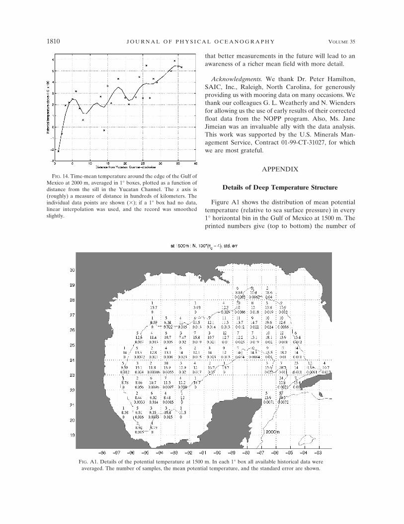
Figure A1 shows the distribution of mean potentialtemperature (relative to sea surface pressure) in every1° horizontal bin in the Gulf of Mexico at 1500 m. Theprinted numbers give (top to bottom) the number of

FIG. A1. Details of the potential temperature at 1500 m. In each 1° box all available historical data wereaveraged. The number of samples, the mean potential temperature, and the standard error are shown.

FIG. 14. Time-mean temperature around the edge of the Gulf ofMexico at 2000 m, averaged in 1° boxes, plotted as a function ofdistance from the sill in the Yucatan Channel. The x axis is(roughly) a measure of distance in hundreds of kilometers. Theindividual data points are shown (�); if a 1° box had no data,linear interpolation was used, and the record was smoothedslightly.


samples, the mean temperature (in excess of 4°C andmultiplied by 100; i.e., 4.123°C would show as 12.3) andthe standard error of the mean. These values include allsamples within 50 m above and below 1500 m. Thesefigures show the data that were used to compile thedata in Table 1. Figure A2 shows the equivalent resultfor 2000 m. Even at these depths, there is a warm cen-tral region in the east and in the west. There also is acooler region along the west coast of Florida and alongthe deep U.S. coast from Louisiana to Texas. The dataare so sparse that constructing temperature contoursseems to require rather more imagination than science.Yet, as compiled in Table 1, the warm center and cooledges seem to be a real feature in the data.

REFERENCES

Bunge, L., J. Ochoa, A. Badan, J. Candela, and J. Sheinbaum,2002: Deep flows in the Yucatan Channel and their relationto changes in the Loop Current extension. J. Geophys. Res.,107, 3233, doi:10.1029/2001JC001256.

Conkright, M. E., and Coauthors, 2000: World ocean database1998. Ocean Climate Laboratory Tech. Rep. 14, NationalOceanographic Data Center, 114 pp.

Davis, R. E., D. C. Webb, L. A. Regier, and J. Dufour, 1992: Theautonomous Lagrangian circulation explorer (ALACE). J.Atmos. Oceanic Technol., 9, 264–285.

Hamilton, P., 1990: Deep currents in the Gulf of Mexico. J. Phys.Oceanogr., 20, 1087–1104.

——, J. J. Singer, E. Waddell, and K. Donohue, 2003: Deepwaterobservations in the northern Gulf of Mexico from in-situ cur-rent meters and PIES. OCS Study MMS 2003-049, Final Re-port to U.S. Minerals Management Service, Vol. 2, Gulf ofMexico OCS Region, 95 pp.

Hofmann, E. E., and S. J. Worley, 1986: An investigation of thecirculation of the Gulf of Mexico. J. Geophys. Res., 91,14 221–14 236.

Johns, W. E., T. L. Townsend, D. M. Fratantoni, and D. Wilson,2002: On the Atlantic Inflow to the Caribbean Sea. Deep-SeaRes., 49, 211–243.

Molinari, R. L., and D. Mayer, 1980: Physical oceanographicconditions at a potential OTEC site in the Gulf ofMexico; 27.5°N, 85.5°W. NOAA Tech. Memo ERL-AOML-42, 100 pp.

——, J. F. Festa, and D. W. Behringer, 1978: The circulation in theGulf of Mexico derived from estimated dynamic height fields.J. Phys. Oceanogr., 8, 987–996.

Niiler, P. P., and W. S. Richardson, 1973: Seasonal variability ofthe Florida Current. J. Mar. Res., 31, 144–167.

Ochoa, J., J. Sheinbaum, A. Badan, J. Candela, and D. Wilson,

FIG. A2. As in Fig. A1 but for 2000 m.


2001: Geostrophy via potential vorticity inversion in theYucatan Channel. J. Mar. Res., 59, 725–747.

Oey, L.-Y., and H.-C. Lee, 2002: Deep eddy energy and topo-graphic Rossby waves in the Gulf of Mexico. J. Phys. Ocean-ogr., 32, 3499–3527.

Schmitz, W. J., Jr., and P. L. Richardson, 1991: On the sources ofthe Florida Current. Deep-Sea Res., 38 (Suppl.), S379–S409.

Sheinbaum, J., J. Candela, A. Badan, and J. Ochoa, 2002: Flowstructure and transport in the Yucatan Channel. Geophys.Res. Lett., 29, 1040, doi:10.1029/GL013990.

Spall, M. A., and J. E. Price, 1998: Mesoscale variability in Den-

mark Strait: The PV outflow hypothesis. J. Phys. Oceanogr.,28, 1598–1623.

Weatherly, G. L., N. Wienders, and A. Romanou, 2005: Interme-diate-depth circulation in the Gulf of Mexico estimated fromdirect measurements. Circulation in the Gulf of Mexico: Ob-servations and Models, Geophys. Monogr., Amer. Geophys.Union, in press.

Wienders, N., G. L. Weatherly, and S. E. Welsh, 2002: Gulf ofMexico 900 meter circulation from PALACE floats. Eos,Trans. Amer. Geophys. Union, 83 (Fall Meeting Suppl.), Ab-stract OS72B-O367.


Documents

Deep Cyclonic Circulation in the Gulf of Mexicosturges/Pubs/DeHaan_SturgesJPO_2005.pdf · from observations, we do not know the deep flow well. Several numerical models include the