Decision Trees & Utility Theory

Michael C. Runge USGS Patuxent Wildlife Research Center

Advanced SDM Practicum

NCTC, 12-16 March 2012

Motivation: Risk

IsSJ

Manage

in situ

Captive

breeding

Introduce to

new island

Persist

Extinct

Ecol.

Damage

Persist

Extinct

Persist

Extinct

Works

Fails

Ecol.

Damage

New Isl.

Augment

Outline

Decision trees

Utility curves

Eliciting utility curves

Utility functions

Multi-attribute utility

Cognitive challenges

A few other thoughts…

Add new technology

to a hatchery?

Does

it

work

?

40,000

Fry

70,000

Fry

10,000

Fry

Decision Tree

Yes

Yes

No

No

p = 0.8

p = 0.2

Actions

Objectives

Model

Yes (0.1)

No (0.9)

Yes (0.7)

No (0.3)

Yes (0.4)

Yes (0.8)

No (0.6)

No (0.2)

Wild Fire? Wet Year? Control Burn?

Yes

Yes (0.1)

No

No (0.9)

No (0.9)

Yes (0.1)

Value

0.70

1.00

0.25

0.35

0.90

0.20

0.10

0.50

0.07

0.90

0.175

0.105

0.36

0.16

0.30

0.02

Wild Fire? Wet Year? Control Burn?

Yes

Yes (0.1)

No

No (0.9)

No (0.9)

Yes (0.1)

0.97

0.28

0.66

0.18

Wet Year? Control Burn?

Yes

Yes (0.1)

No

No (0.9)

No (0.9)

Yes (0.1)

Wet Year? Control Burn?

Yes

0.097

No

0.252

0.162

0.066

Control Burn?

Yes

No

0.349

0.228

Roll-back Method:

Start at right

EV at chance nodes

Best at choice nodes

Move left until done

Does EV capture values?

Choice

Game

1

$30

-$1

Game

2

$2000

-$1900 Expected values

Game 1: $14.50 Game 2: $50.00

Which do you choose?

Expected Value

The expected value criterion

• Assumes a long-run average

• Assumes a linear value function

• Focuses on only a single attribute

But maybe…

• We make repeated decisions in our

life…

Risk Attitude

Consider the following wager • Win $500 with prob 0.5, or lose $500 with prob 0.5

• Would you pay to get out of this wager? How much?

• Would you pay to get into this wager? How much?

A classic risk decision

$500

Win

? Yes

Yes

No

No

p=0.5

EV = ?

EV = $0

Bet?

p=0.5 -$500

-$?

Risk Attitude

Risk-averse • You would trade a gamble for a sure amount that is

less than the expected value of the gamble

• E.g., buying insurance

Risk-seeking • You would trade a sure amount for a gamble that

has a smaller expected value (but the chance of a larger payout)

• E.g., buying lottery tickets

Add new technology

to a hatchery?

Does

it

work

?

40,000

Fry

70,000

Fry

10,000

Fry

Decision Tree

Yes

Yes

No

No

p = 0.8

p = 0.2

EV = 40K

EV = 58K

Utility

0 20 40 60 80 0.00

0.25

0.50

0.75

1.00

Hatchery production (1000s)

Utilit

y

Add new technology

to a hatchery?

Does

it

work

?

40,000

Fry

70,000

Fry

10,000

Fry

Risk-averse Utility

Yes

Yes

No

No

p = 0.8

p = 0.2

EU = 0.9

EU = 0.8

U = 1.0

U = 0.0

U = 0.9

Trade a gamble with

expected value of 58K

for a sure thing with a

value of 40K

Properties of Utility Functions

Monotonic vs. peaked

Risk tolerance

• Averse, neutral, seeking

• Mixed

Constant vs. declining aversion

Eliciting Utilities

Elicitation methods center around gamble choices • Notation: [x, , y] R w

• The choice is between a sure return of w or gamble that returns x with probability or y with probability 1

• R is the preference relation (, , or ~)

Lottery diagram

x

Choice

y

w

1

Methods of Elicitation

Preference comparison • [xi, i, yi] Ri wi

Probability equivalence • [xn+1, i, x0] ~ xi

Value equivalence

Certainty equivalence • [x*, 0.5, x0] ~ x1, [x1, x0] ~ x2, [x*, x1] ~ x3,…

Probability-equivalence

w -10,000 0 10,000 30,000 60,000

u(w) 0.0 1.0

60,000

Choice

-10,000

w

Probability-equivalence

w -10,000 0 10,000 30,000 60,000

0.85

u(w) 0.0 1.0

60,000

Choice

-10,000

w

Probability-equivalence

w -10,000 0 10,000 30,000 60,000

0.60 0.85

u(w) 0.0 1.0

60,000

Choice

-10,000

w

Probability-equivalence

w -10,000 0 10,000 30,000 60,000

0.35 0.60 0.85

u(w) 0.0 1.0

60,000

Choice

-10,000

w

𝑢 30,000 = 𝛼𝑢 60,000 + 1 − 𝛼 𝑢 −10,000

= 𝛼 1.0 + 1 − 𝛼 0.0 = 𝛼

Probability-equivalence

w -10,000 0 10,000 30,000 60,000

0.35 0.60 0.85

u(w) 0.0 0.35 0.60 0.85 1.0

60,000

Choice

-10,000

w

𝑢 30,000 = 𝛼𝑢 60,000 + 1 − 𝛼 𝑢 −10,000

= 𝛼 1.0 + 1 − 𝛼 0.0 = 𝛼

Utility Curve

0

0.2

0.4

0.6

0.8

1

1.2

-10000 0 10000 20000 30000 40000 50000 60000

Uti

lity

Payoff ($)

Certainty-equivalence

x 60,000

y -10,000

w w1

u(w)

x 0.5

Choice

y

w

𝑢 𝑤1 = 0.5𝑢 60,000 + 1 − 0.5 𝑢 −10,000

= 0.5 1.0 + 0.5 0.0 = 0.5

Certainty-equivalence

x 60,000 w1

y -10,000 -10,000

w w1 w2

u(w) 0.5

x 0.5

Choice

y

w

𝑢 𝑤2 = 0.5𝑢 𝑤1 + 1 − 0.5 𝑢 −10,000

= 0.5 0.5 + 0.5 0.0 = 0.25

Certainty-equivalence

x 60,000 w1 60,000 60,000 w3 w1 w2

y -10,000 -10,000 w1 w3 w1 w2 -10,000

w w1 w2 w3

u(w) 0.5 0.25 0.75

x 0.5

Choice

y

w

𝑢 𝑤3 = 0.5𝑢 60,000 + 1 − 0.5 𝑢 𝑤1

= 0.5 1.0 + 0.5 0.5 = 0.75

Certainty-equivalence

x 60,000 w1 60,000 60,000 w3 w1 w2

y -10,000 -10,000 w1 w3 w1 w2 -10,000

w w1 w2 w3

u(w) 0.5 0.25 0.75 0.875 0.625 0.375 0.125

x 0.5

Choice

y

w

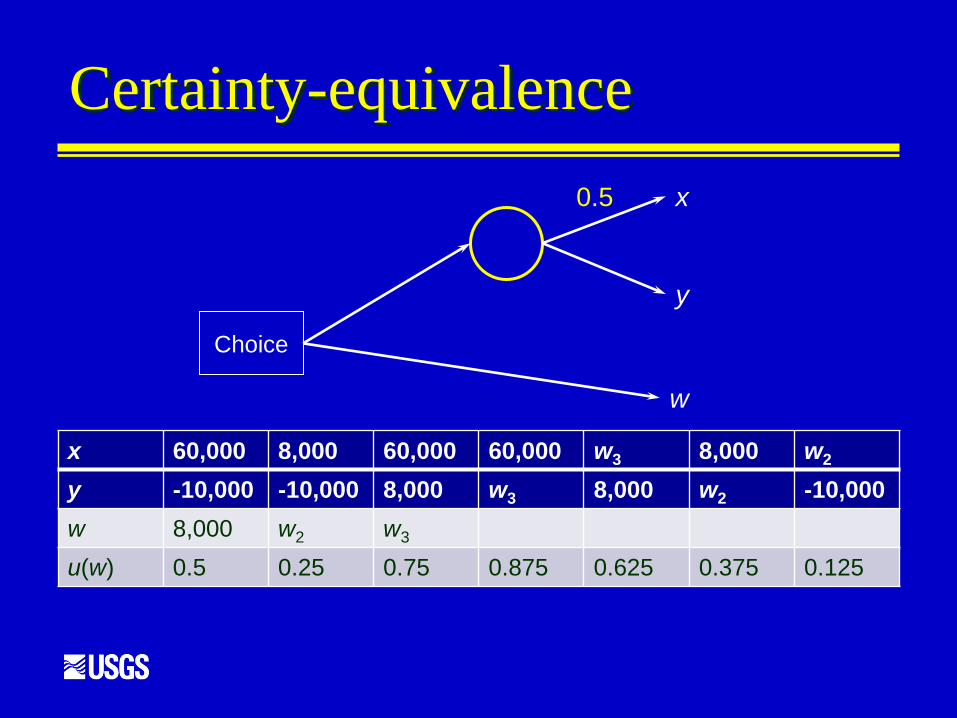
Certainty-equivalence

x 60,000 8,000 60,000 60,000 w3 8,000 w2

y -10,000 -10,000 8,000 w3 8,000 w2 -10,000

w 8,000 w2 w3

u(w) 0.5 0.25 0.75 0.875 0.625 0.375 0.125

x 0.5

Choice

y

w

Certainty-equivalence

x 60,000 8,000 60,000 60,000 w3 8,000 2,000

y -10,000 -10,000 8,000 w3 8,000 2,000 -10,000

w 8,000 -2,000 w3

u(w) 0.5 0.25 0.75 0.875 0.625 0.375 0.125

x 0.5

Choice

y

w

Certainty-equivalence

x 60,000 8,000 60,000 60,000 20,000 8,000 2,000

y -10,000 -10,000 8,000 20,000 8,000 2,000 -10,000

w 8,000 -2,000 20,000

u(w) 0.5 0.25 0.75 0.875 0.625 0.375 0.125

x 0.5

Choice

y

w

Certainty-equivalence

x 60,000 8,000 60,000 60,000 20,000 8,000 2,000

y -10,000 -10,000 8,000 20,000 8,000 2,000 -10,000

w 8,000 -2,000 20,000 32,000

u(w) 0.5 0.25 0.75 0.875 0.625 0.375 0.125

x 0.5

Choice

y

w

Certainty-equivalence

x 60,000 8,000 60,000 60,000 20,000 8,000 2,000

y -10,000 -10,000 8,000 20,000 8,000 2,000 -10,000

w 8,000 -2,000 20,000 32,000 12,000 4,000 -5,000

u(w) 0.5 0.25 0.75 0.875 0.625 0.375 0.125

x 0.5

Choice

y

w

Utility Curve

0

0.2

0.4

0.6

0.8

1

1.2

-10000 0 10000 20000 30000 40000 50000 60000

Uti

lity

Payoff ($)

Methods of Elicitation

Preference comparison • [xi, i, yi] Ri wi

Probability equivalence • [xn+1, i, x0] ~ xi

Value equivalence

Certainty equivalence • [x*, 0.5, x0] ~ x1, [x1, x0] ~ x2, [x*, x1] ~ x3,…

Utility Functions

There are functions that describe smooth utility

curves

• Compact expressions

• These are often easier to elicit than a lot of

individual points

Common

• Linear

• Exponential

• Logarithmic

Exponential Utility

0

0.2

0.4

0.6

0.8

1

1.2

0 0.5 1

Y-Values Kernel

• 𝑒−𝑐𝑥

Risk attitude

• c>0, risk averse

• c<0, risk seeking

• constant

Logarithmic Utility

0

0.2

0.4

0.6

0.8

1

1.2

0 0.5 1

Y-Values Kernel

• log (𝑥 + 𝑏)

• x > b

Risk attitude

• risk averse

• declining

Scaling

Utility functions can be scaled to the

interval {0,1}

• Linear transformation

𝑢 𝑥 =𝑘 𝑥 −𝑘(𝑥0)

𝑘 𝑥1 −𝑘(𝑥0)

Multi-attribute Utility

What if there is more than one

objective?

Most commonly

• Assume mutual utility independence

• Develop utilities separately

• Combine into single expression

Goodwin & Wright (2004:123ff)

Cognitive Challenges

Lotteries are imaginary

Subtleties of elicitation

• Gift, purchase, sale, transfer

Strength of preference for sure

outcomes vs. attitudes toward risk

Recommendations

Pre-analysis preparation phase

• Motivate decision maker to think

carefully about responses

Use more than one assessment

procedure

Phrase utility questions in terms

closely related to original problem

A few more thoughts…

Value vs. utility

“Unknown unknowns”