Decision Support System for Evaluating Rural Water Supply

Infrastructure Scenarios

Art Stoecker

Department of Agricultural Economics

312 Ag Hall

Oklahoma State University

Stillwater, Oklahoma 74074

Ph: (405) 744-6165

art.stoecker@okstate.edu

Dee Ann Sanders

Department of Civil Engineering

Oklahoma State University

deeann.sanders@okstate.edu

Brian E. Whitacre

Department of Agricultural Economics

Oklahoma State University

brian.whitacre@okstate.edu

Selected Paper prepared for presentation at the Southern Agricultural Economics Association

Annual Meeting, Orlando, FL, February 6-9, 2010

Copyright 2010 by Art Stoecker, Dee Ann Sanders, and Brian E. Whitacre. All rights reserved.

Readers may make verbatim copies of this document for non-commercial purposes by any

means, provided that this copyright notice appears on all such copies.

1

Introduction

Rural water systems often struggle to make decisions regarding their future, particularly

when those decisions involve upgrading their infrastructure or consolidating / cooperating with

other systems. This paper demonstrates the development of a step-by-step methodology that

provides assistance to rural water systems for planning and updating their water supply

infrastructure. The direct connection between the research methods and extension tools used are

a unique component of the project, as contact and discussion with rural water system personnel

was essential for project completion. The methodology is generalizable to any number of rural

water systems, including those using either surface or groundwater. While we initially hoped the

tools and methods used under this methodology would be able to be performed by non-

specialists, such as local water district managers, our experience indicates that some specialist

oversight is likely necessary. This system of evaluation should still dramatically enhance the

capability of rural water districts to understand the limitations of their current system and give

updates to the local community well in advance of any infrastructure crisis.

Background of Project

The 2007 Environmental Protection Agency (EPA) report of Drinking Water

Infrastructure Needs Survey and Assessment stated that the United States would need an

investment of about 335 billion dollars to upgrade its water infrastructure in the coming 20 years.

The report said that out of this entire revenue, 60% would be required for just upgrading the

distribution systems. The state-by-state classification of the report said that Oklahoma would

need about 2.6 billion dollars, out of which 1.4 billion dollars would be required to upgrade the

systems serving populations fewer than 3300 people (EPA, 2007). The Oklahoma Water

2

Resources Board (OWRB) set a new water plan to project water demands and the required

inventory to meet these demands up to the year 2060. The preliminary goals of this project were

as follows: (OWRB, 2009)

Identify those regions having problems related to water supply

Collect data, maps and other vital information regarding their water infrastructure

Evaluate the performance of their systems on the basis of existing demands

Identify the necessary changes in the system to meet future water demands.

OWRB identified 1717 active public water systems, out of which 1240 systems were

community water systems, either municipal or rural water districts. Partners in this planning

process were the Oklahoma Water Resources Research Institute, the Oklahoma Association of

Regional Councils (COG’s), Oklahoma Department of Environmental Quality (ODEQ) and

federal partners. Based on the water plan for Oklahoma, a project goal was set to develop a cost

efficient methodology, which would assist rural water districts in Oklahoma to manage and

upgrade their drinking water distribution systems. Four rural water systems were chosen,

representing systems with above ground storage, below ground storage, groundwater sources,

and surface water sources. The four systems chosen were Beggs, Oklahoma, Braggs, Oklahoma,

Kaw City, and Oilton, Oklahoma. These systems represented a variety of infrastructure issues,

including insufficient storage, old pipes, and low pressure areas. In addition to the options in the

systems selected, two different water distribution models were used during the project. The

locations of the towns are shown in Figure 1 while the population, source of water, and general

problems for these towns is given in Table 1.

3

Figure 1. Location of Study Site Towns of Beggs, Braggs, Kaw City, and Oilton in Oklahoma

Table 1. Small Towns in Oklahoma Participating in Study of Water System Planning.

Item Beggs Braggs Kaw City Oilton

Population 1,364 1,030 400 1,200

Water Source S.W. G.W. G.W. G.W.

Gallons/Day (thos) 161 75.6 80 118

Treatment Conventional. NR NR NR

Storage (thos. gal.) 175b 200 200 950

Issues: Old pipes yes Yes Yes

Insufficient storage Yes No Yesc No

Low Pressure Areas yes yes No yes

Sufficient Fire Flow No Yes Yes No

Primary Standards ok ok ok ok

Secondary Standards ok ok Mn ok

Water Age Somed Some

d Some

d Some

d

a Abbreviations used; S.W. = surface water, G.W. = ground water, NR = not required.

b 50,000 elevated plus 125,000 in ground tank.

c During summer tourist weekends.

d Generally in areas served by long un-looped pipes

The Kaw City System study involves potential regionalization of water treatment systems

and has not been completed. Only one of the four towns had digital pipeline data set. In some

cases, the hand drawn pipeline maps were incomplete. The approach in this study was to

develop a hydrological simulation model for the town and then use that model to address the

problems shown above in Table 1. The following approach was followed.

4

1) Contact and meet with appropriate local officials such as the mayor, manager, and/or

city engineer.

2) Obtain copies of pipe line maps noting length, diameter, age, material, and condition,

if possible. Alternatively sketch pipeline maps onto Google or Tiger line drawings of

the city. Handheld GPS units were used to verify the location of critical infrastructure

such as wells, treatment plants, and water storage units.

3) Obtain available technical information about the pumps, (size, power, model, age,

power consumption, and hours of operation) and other system components.

4) Develop and validate an EPANET or WaterCAD simulation model for the water

system.

5) Use the EPANET or WaterCAD models to evaluate the ability of the system to meet

time of day demands by spatial location. The EPANET hydrological simulation

program was developed by EPA and is available at no cost. WaterCAD is a

commercial system distributed by Bentley Systems.

6) Determine the ability of the water distribution system to meet fire flow demands at

each hydrant (minimum 20 psi after two hours of 250 gpm flow).

7) Evaluate the type, amount, and time of infrastructure needs to meet projected

population growth.

Simulation Model Development

The Oklahoma Water Resources Board (OWRB) has developed a set of GIS pipeline

drawings for some 800 rural water systems in Oklahoma; however, these drawings typically do

not include small towns such as the ones included in this project. The first step was to develop

the geographical information system (GIS) drawings of the major pipelines serving the city.

Zonum Systems (2009) has developed several freeware interfaces to EPANET. One program,

(EPANETZ) allows the user to digitize pipelines onto a Google Map of the town. Comparison

of the Google map of the town with engineering drawings permits development of a digital

infrastructure map with approximate (though not exact) location of pipelines. The program

automatically creates the necessary linkages between nodes. The user must enter the pipe

diameters and the node elevations. The GIS will provide estimates of the length of pipes, but

actual lengths should be used when these are available. Two or more pipes are considered joined

5

if they share the same node. One problem in getting EPANET to operate, is that slight

differences in placement of pipe lines may generate multiple nodes which appear as a single

node on one location. More expensive simulation programs link such nodes automatically.

Excel macros were written to check the differences in latitude and longitude between nodes and

ask the user if pipes having separate ending nodes within a specified radius should be connected,

essentially requiring user verification for each unconnected node.

A second problem encountered was how to determine the elevation of each node, which

is a required input for determining water flow. This is difficult for inexperienced users to

accomplish in ARCVIEW or ARCMAP. However, a second relatively inexpensive GIS

program, Global Mapper, was available that creates XYZ files (which include elevation) by

simply overlaying the line drawing of the pipes on a USGS elevation file. Visual Basic macros

were then used to add the elevations to the pipeline nodes. (Zonum Solutions (2009) now offers

an online program to add elevations to nodes). The values relating to the depth of wells, height

and volume of storage facilities, pump curves, rules for pump operation, and diurnal water use

patterns must be added to the data set. The effect of corrosion in reducing pipe flows was also

approximated after discussions with the city engineer.

The following three sections discuss the steps taken to evaluation the distribution systems

in Beggs, Oilton, and Braggs, respectively. As indicated, free EPANET software was used in

both Beggs and Braggs, while Oilton incorporated the for-fee WaterCAD software typically used

by professional engineers. A discussion of the issues faced during each simulation is included.

Additionally, the analysis of Beggs (which was completed prior to Oilton and Braggs)

incorporates a methodology for assessing the cost of potential upgrades to the existing

infrastructure.

6

Simulation Model to Evaluate the Beggs Water Distribution System

The EPANET model developed for the City of Beggs will be used to illustrate the

capabilities of the water simulation software to analyze problems and possible solutions for a

small town (Lea, 2009).

Figure 2 shows the digitized pipeline for the City of Beggs overlaid on photo map of the

city. The low pressure areas indicated by circles along with the areas where the age of water in

the pipes was problematic on Figure 2 were confirmed by the city engineer. One area with

pressure problems and inadequate fire flow was on the west end where the primary and

secondary schools were located. A similar problem was encountered with the “Hilltop” area on

the east. Both of these areas represent city expansions made after the initial water system was

developed. The dead ends associated with several long pipes also failed the fire-flow test.

7

Figure 2. Digitized EPANET Model of the Water System for Beggs, Oklahoma Showing

Pipeline Flow and Indications of Areas with Low Pressure and Areas Where Age of Water in the

Pipes was Problematic.

The alternatives simulated to correct the problems shown in Figure 2 included installing

new or modified pumps, a new water tower on the east end of town, replacing old pipes that had

corrosive deposits, and / or adding new pipes to eliminate dead ends and create new water paths.

A set of simulations involving the addition of new pipes to convert the long single pipes

shown in Figure 2 into loops indicated the problem of water age could be remedied most of the

pressure and fire flow problems could be resolved. The pipes and water tower added during the

simulations are shown in Figure 3.

8

Figure 3. EPANET Model of the Water System for Beggs with Pipes added to Eliminate Dead

Ends and the Location of a New Water Tower.

An important issue for a small town like Beggs, which is currently facing sewer upgrade

problems, is the cost and the best order in which make modifications.

Cost estimates for pipe, pumps, and storage tanks were obtained from Means (2009) and

adjusted were necessary to account for price changes since publication. Table 2 shows the prices

used to the cost of installing PVC pipe of alternative diameters. A spreadsheet was used to

develop the cost for the purchase and installation cost of alternative sizes of PVC pipe from 2

through 8 inches, using data on the cost of pipe, excavation, and backfilling used estimates from

Means (2009).

9

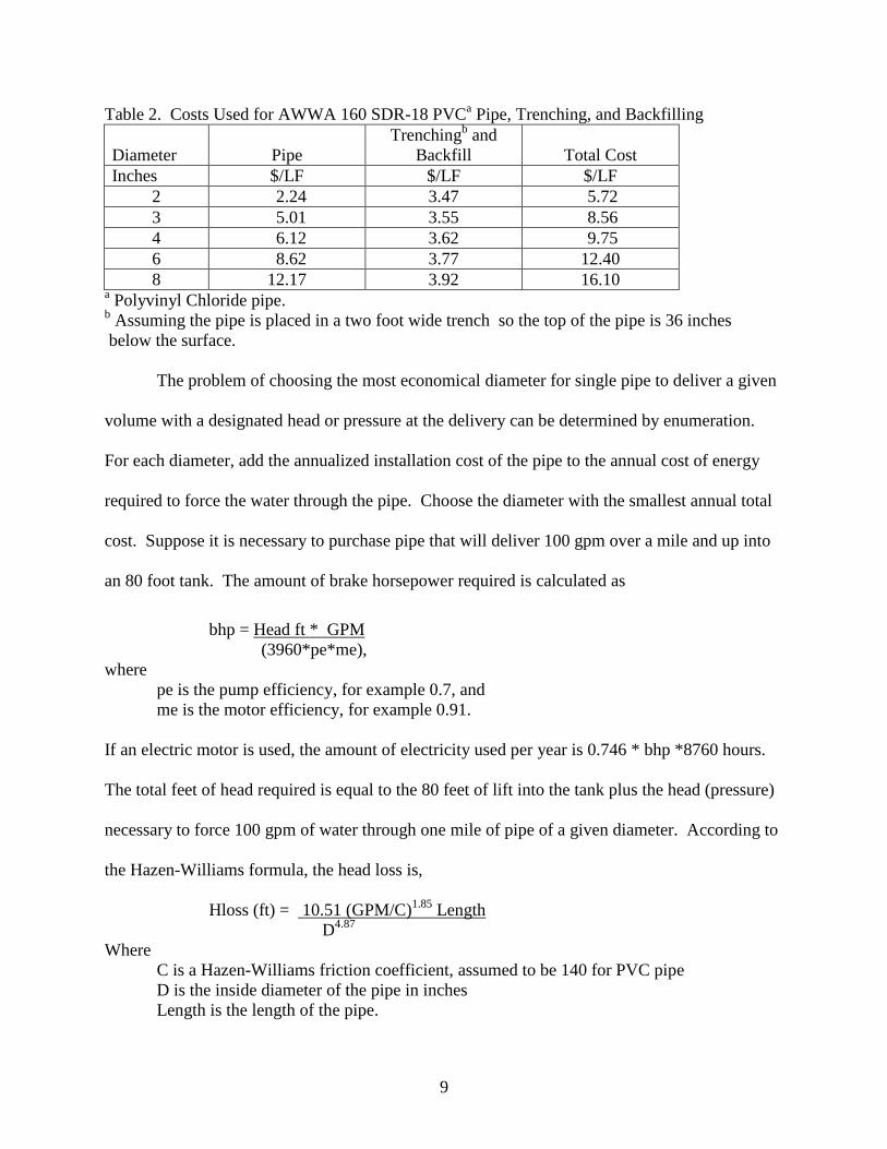
Table 2. Costs Used for AWWA 160 SDR-18 PVCa Pipe, Trenching, and Backfilling

Diameter Pipe

Trenchingb and

Backfill Total Cost

Inches $/LF $/LF $/LF

2 2.24 3.47 5.72

3 5.01 3.55 8.56

4 6.12 3.62 9.75

6 8.62 3.77 12.40

8 12.17 3.92 16.10 a Polyvinyl Chloride pipe.

b Assuming the pipe is placed in a two foot wide trench so the top of the pipe is 36 inches

below the surface.

The problem of choosing the most economical diameter for single pipe to deliver a given

volume with a designated head or pressure at the delivery can be determined by enumeration.

For each diameter, add the annualized installation cost of the pipe to the annual cost of energy

required to force the water through the pipe. Choose the diameter with the smallest annual total

cost. Suppose it is necessary to purchase pipe that will deliver 100 gpm over a mile and up into

an 80 foot tank. The amount of brake horsepower required is calculated as

bhp = Head ft * GPM

(3960*pe*me),

where

pe is the pump efficiency, for example 0.7, and

me is the motor efficiency, for example 0.91.

If an electric motor is used, the amount of electricity used per year is 0.746 * bhp *8760 hours.

The total feet of head required is equal to the 80 feet of lift into the tank plus the head (pressure)

necessary to force 100 gpm of water through one mile of pipe of a given diameter. According to

the Hazen-Williams formula, the head loss is,

Hloss (ft) = 10.51 (GPM/C)1.85

Length

D4.87

Where

C is a Hazen-Williams friction coefficient, assumed to be 140 for PVC pipe

D is the inside diameter of the pipe in inches

Length is the length of the pipe.

10

The minimum annual cost involves a tradeoff between pipe size and energy cost. As the

diameter of the pipe increases, the total cost of the pipe increases, but the energy required to

force the water through the pipe decreases. A standard capital recovery factor was used to

annualize the cost of the pipe. The annual capital cost for one mile of pipe (Table 2) and the

annual pumping costs are added together in Figure 4. The least cost alternative is the four-inch

diameter pipe that would cost $7,000 per year.

Figure 4. Comparison of Annual Total, Capital, and Energy Cost to Install One Mile of PVC

Pipe with a 20-year Life to Deliver 100 GPM to an 80 Foot Tank when Electricity Costs are

$0.10 per kwh and the Interest Rate is Five Percent..

However, in a water system the problem is more complicated since a new pipe will be

used in a net work with other pipes. Also, Oklahoma mandates require that if a fire hydrant is

attached to the pipe, the minimum diameter would have to be six inches. Alternative simulation

runs were used to compare the system performance in terms of pressures and energy cost before

and after each change in the distribution system infrastructure. The capital costs associated with

different solutions were calculated outside the simulation.

11

The ability to meet fire flow requirements at each fire hydrant node was tested by adding

a 250 gpm demand to each node in turn and testing the pressure after a two hour simulation. The

full set of fire node tests were repeated after each set of infrastructure changes. Excel macros

were again used to write out the simulation input data, run the simulation, retrieve the results of

each simulation, and determine the number of fire flow and other failures in the system. A set of

incremental infrastructure investments was developed that maximized the number of new fire

hydrant nodes meeting the fire flow test per dollar spent. The results are shown in Table 3. In

Table 3, the greatest initial improvement per investment dollar came from adding the two major

pipes in the eastern part of Beggs. At the bottom of Table 3, the additional water tower in

eastern Beggs, added onto the previous changes, had the fewest improvements per dollar spent.

Table 3. Order of Changes in Beggs Water Distribution System to Maximize Fire-Flow

Compliance per Dollar Invested.

Order Description of Changes Cost

1 Install two major pipes in East Beggs $ 69,000

2 Add three additional pipes in East Beggs to finish addressing Hilltop pressure problems

$ 60,000

3 Add remaining pipes to eliminate targeted dead ends $ 57,000

4 Add Additional Fire Hydrants $ 60,500

5 Add 50,000 gallon water tower in East Beggs $ 167,000

Total All Changes $ 415,000

Site description of Oilton, Oklahoma

The City of Oilton is located in Creek County and is approximately 54.6 miles to the west

of Tulsa. Located close to the Cimarron River, the city of Oilton houses a small community

having a population of about 1200 people. The approximate area of the city is 0.65 square miles,

which is about 416 acres. The City of Oilton receives its water supply through groundwater. The

system has two wells that are located five miles to the south of the city. The storage facilities

used by the town are two standpipe tanks. One tank is located outside the city and the other tank

12

is located in the city. The exact age of the pipelines is not known. The main pipeline that brings

water to the city is an eight-inch asbestos cement pipeline. There are two main distribution pipes

in the town, one of which is an eight-inch PVC pipeline while the other is an 8 inch asbestos

cement pipeline. All other mains and sub-mains are in the range of 1 to 6 inches. A summary of

the statistics of the Oilton water distribution system is shown below in Table 5. Figure 1 shows

the map of the town. Figure 2 shows a schematic of the distribution system.

Table 4: Oilton System Statistics

• Source: 2 deep (approx. 500 ft) wells

• Pumps: Single submersible pump per well

• Total Storage: 950,000 gal

• Pumping Rate: 118,000 gal/day (81 gpm)

• Population Served: 1200

Selection of hydraulic simulation software for Oilton, Oklahoma

The hydraulic simulation software used for this part of the study was WaterCAD V8i

distributed by Bentley Systems. The aim was this project was to provide an economic tool which

would be affordable to rural water districts. However, after completion of the previous study

carried out for the Beggs water system, it was evident that the free hydraulic simulation software

used (EPANET) was too sophisticated to be handled and updated by the rural water districts’

staff.

Thus this project has a demonstration approach. WaterCAD V8i was selected due to ease of

model building and operation and its greater programming capabilities as compared to EPANET.

Although rural water system personnel are not likely to be able to use WaterCAD, most

13

professional civil engineers do have knowledge of the software and a demonstration of its

applicability to rural systems can potentially aid future efforts to assist these communities.

FIGURE 5: Map of Oilton, Oklahoma, Area (Google Maps, 2009)

To use the simulation software, the following steps were followed:

1. Pipelines were digitized, from information gathered on location (x-y coordinates), length,

and diameter.

2. Facilities were located, including treatment plants, wells, pumps, and towers/standpipes.

3. Unknowns at this point included

Elevation Changes along pipeline

Location of Users along pipeline

14

Demand allocation along pipeline

Age, Condition, Materials

FIGURE 6: Schematic of Oilton, Oklahoma, Water Distribution System (Bhadbhade, 2009)

Apart from the preliminary information, additional inputs were required for the

simulation of the model. The most important was the elevation dataset. Without the elevations, it

is not possible to run the hydraulic simulation. The elevation dataset was obtained from the

United States Department of Agriculture (USDA) website called the “Geospatial Data Gateway”

(USDA, 2009). Note that this elevation data source is different than that used for the Beggs

simulation. The second important dataset necessary was the information regarding houses in

15

each census block. This information is required to assign base water demands to each node. The

census block data was obtained from the US Census Bureau website called the “2008

TIGER/Line Shapefiles”. The user can select the respective state and county, and the Census

2000 Block data was used to match households to potential nodes. Again, the USDA Geospatial

data Gateway website was used to download the ortho-images of Oilton for identification of the

houses in each census block.

Oilton Simulation Results

• Very large storage results in long water age and excessively long (several days) pump

cycles to fill the tanks.

• However, most storage volume is unusable due to low pressures that result when water in

standpipes is dropped more than 30 ft from the top of the tanks.

• Excessively long, low-demand lines result in high water age and low disinfectant

residuals at dead ends.

Site description of Braggs, Oklahoma

Braggs is located in eastern Oklahoma, 56 miles south east of Tulsa (Figure 7). The

population of the city is 308. The largest section of the existing water distribution system was

installed in 1982 and has been serving the local population and 650 people in surrounding areas

for the last 27 years.

16

BRAGGS, OKLAHOMA

FIGURE 7: Map of the Braggs, Oklahoma, area (Google Maps, 2009)

Currently the system has 416 service connections and serves 1030 people from its

primary water source which is ground water artesian wells. The distribution system network

consists of three water towers; one located in the center, one at the north end and one on the

south end of the city, giving a total storage capacity of 200,000 gallons.. A summary of the

statistics for the Bragg distribution system is shown in Table 5.

Table 5: Braggs System Statistics

• Source: Artesian Wells

• Pumps: 3 identical working in parallel

• Total Storage: 200,000 gal

• Pumping Rate: 75,600 gal/day (52.5 gpm)

• Service Connections: 416

• Population Served: 1030

17

The piping consists mainly of long two inch branches pipes which are interconnected by a few

four and six inch supply mains.

The map of the Braggs water distribution system was obtained from the Water

Information Mapping System (WIMS) on the Oklahoma Water Resources Board (OWRB)

website at http://www.owrb.ok.gov/maps/server/wims.php. WIMS is an Internet-based map

server that requires a supported web browser. The Braggs system is shown in Figure 8.

FIGURE 8: Schematic of Water Distribution Pipelines in Braggs, Oklahoma,

Service Area from EPANETZ

18

Information regarding the age of the system, problems related to inadequate flows, low

water pressure, leakages and bursts water usage patterns and equipment information for pumps

was obtained from interviews with the plant operator at Braggs, Oklahoma. Water usage data

were obtained from the Oklahoma Department of Environmental Quality (ODEQ) records. The

records included information regarding the total water pumped daily from the treatment plant,

the pH and the doses of the different chemicals added to the water prior to distribution over an

eight year period from January 2001 to April 2009.

Hydraulic modeling using EPANET for Braggs, Oklahoma

The process of modeling a network using EPANET involves input of the parameters or

variables that most closely describe the operation of the actual system. These parameters include

the shape of the tanks, the pump curve which describes the operation of the pump and an infinite

reservoir. Other input parameters required for the model to run include the maximum and

minimum water levels and an initial water level in the tank. The three water tanks at Braggs are

all cylindrical in shape.

There are three identical pumps at Braggs, each delivering 150gpm at 208ft of head. The

pumps operate in parallel delivering the same head and are set to sequentially come on line in

order to meet increasing flow requirements for the system. The pumps were modeled according

to the information received from the system operator. Usually a single pump is switched on

when the pressure drops below 65psi and is switched off when the pressure exceeds 80psi.

Therefore, rule based controls were set within the EPANET model to ensure that the first pump

was switched on when the pressure dropped below 65psi and switched off when the pressure

increased to 80psi. Pump 2 was modeled to switch on if the pressure dropped further as would be

19

the case in the event of a fire. Pump 3 was treated as a standby for the system in case pumps 1 or

2 failed to operate and was not included in the hydraulic modeling process.

The greatest percentage of the pipes at Braggs were installed in 1982 when the currently

existing PVC pipes were installed to replace deteriorated cast iron pipes that had been previously

installed in the 1940’s. Therefore, most of the pipes are almost 30 years old. The operator noted

that they had not replaced any pipes recently.

Braggs Simulation Results

• Technical work necessary to use the EPA Net software took several months. The

software is not user friendly and technical support is non-existent.

• Relatively good records from the operator resulted in good match between simulation and

the limited physical system measures (flows and pressures).

• Water age was high and disinfectant residual was predicted to be low in the long dead

ends. Looping did not help, since it merely increased the flow paths and further lowered

velocities.

Overall Project Conclusions

The project was successful in constructing a methodology to evaluate rural water system

infrastructure. The incorporation of different water sources, infrastructure issues, and modeling

software indicates that several approaches can be taken to effectively help rural water systems

plan and update their water supply infrastructure. The development of a cost estimating

methodology was also an essential part of the project, since understanding the costs associated

with different upgrades is important for the community to understand. Highlights of the project

results include:

20

• Small systems have common problems of low demand and long, low-velocity lines,

which result in high water age and low disinfectant residual.

• The common remedy for high water age, which is to loop the pipes, does not always

work for small systems, due to very low demand. A loop will add even more length to an

already excessively-long system.

• Elevation differences mean that some areas have high pressures while others have very

low (sometimes unacceptable) pressures.

• Technical expertise and experience necessary to use either EPA Net or WaterCAD are

beyond the staffing capabilities of small systems. It took several months for engineering

graduate students to become familiar with the software.

• Small communities need assistance in writing grants to get funding for system

improvements. Just getting a grant written is beyond the capability of most system staff

members.

To this last point, each of the communities participating in the project expressed anxiety

about paying for the upgrades suggested by the simulations. Discussions with OWRB personnel

indicate that significant effort has already taken place to educate rural water district personnel

about requirements for applying for funding, including a multitude of fact sheets and even a

yearly full-day conference sponsored by the Funding Agency Coordinating Team (advertised as

“one stop shopping to find the financing you need for your project” (Oklahoma Rural Water

Association, 2009)). Our experience suggests the promotion of this type of event is crucial, as is

the technical help provided by “Circuit Riders” who travel to small water systems and provide

educational sessions for system personnel. Finally, the need for professional engineering help

indicates that an extension program (provided by any land-grant university) focused on this area

21

would be in high demand, particularly for states with many rural water systems. Funding a full-

time engineer to deal with projects such as those explored in this paper would provide significant

benefit for the rural water systems assisted and would likely result in extremely positive publicity

for the departments involved.

References

Bhadbhade, Neha (2009) Performance Evaluation of a Drinking Water Distribution System

Using Hydraulic Simulation Software for the City of Oilton, Oklahoma.Masters’ Thesis,

Oklahoma State University, Stillwater, Oklahoma.

Environmental Protection Agency (2007). “Drinking water Infrastructure Needs Survey and

Assessment Fourth Report to Congress”. Retrieved on September 29th

2009 from

http://www.epa.gov/ogwdw000/needssurvey/pdfs/2007/report_needssurvey_2007.pdf

Environmental Protection Agency (2009) Software that Models the Hydraulic and Water Quality

Behavior of Water Distribution Piping Systems. U. S. Environmental Protection Agency.

Accessed 2009. Software and user manuals available at,

http://www.epa.gov/NRMRL/wswrd/dw/epanet.html

Google Maps (2009), found at http://maps.google.com.

Lea, M. C. (2009). Use of Hydraulic Simulation Software to Evaluate Future Infrastructure

Upgrades for a Municipal Water Distribution System in Beggs, Oklahoma, Masters’

Thesis, Oklahoma State University, Stillwater, Oklahoma.

Oklahoma Rural Water Association (2009). February 2009 Newsletter. Found at:

http://okruralwater.org/Updates/feb09update.pdf

Oklahoma Water Resources Board (OWRB) (2009), OWRB Website, found at

http://www.owrb.ok.gov/.

R.S. Means Company, Inc. (2009) Facilities Construction Cost Data, 24’th Edition, R.S. Means

Company, Inc, Construction Publishers and Consultants, Kingston, Ma.

Senyondo, Sara (2009) Using EPANET to Optimize Operation of the Rural Water Distribution

System at Braggs, Oklahoma, Masters’ Thesis, Oklahoma State University, Stillwater,

Oklahoma.

Zonum Solutions. (2009). Free Software Tools: EPANET-Z. Zonum Solutions, Arizona,

Software available at http://www.zonums.com/epanet_cat.html