Dealer Funding Costs: Implications for the Term

Structure of Dividend Risk Premia

Yang Song∗

Abstract

I show how funding costs to derivatives dealers’ shareholders for carrying and hedg-

ing inventory affect mid-market derivatives prices. An implication is that some sup-

posed “no-arbitrage” pricing relationships, such as put-call parity, frequently break

down. As a result, I show that risk premia for S&P 500 dividend strips estimated in

some recent research are notably biased. In particular, I question whether the term

structure of S&P 500 dividend risk premia is on average downward sloping.

∗Graduate School of Business, Stanford University. Email: songy@stanford.edu. I am especially indebtedto Darrell Duffie for numerous discussions and comments. I am grateful to Yu An, Jules van Binsbergen,Svetlana Bryzgalova, John Cochrane, Zhiguo He, Zhengyang Jiang, Arvind Krishnamurthy, Hanno Lustig,Tim McQuade, Teng Qin, Ken Singleton, and Amir Yaron for valuable feedback. All remaining errors areof course my own.

1

I. Introduction

Recent research estimates equity dividend risk premia by relying on put-call parity to

infer the prices of equity dividend strips. I show that dividend strip prices should instead

be inferred using an adjustment to the put-call parity formula. This adjustment, for the

spread between the equity repo rate and the risk-free market interest rate, reflects the cost

to dealers of financing their equity hedges in the repo market. In particular, I question the

method used by van Binsbergen, Brandt, and Koijen (2012) to estimate S&P 500 dividend

risk premia, and whether this term structure is on average downward sloping.

Options dealers, acting as intermediaries, provide immediacy to ultimate investors by

temporarily absorbing their net trade demands. In doing so, dealers have net funding re-

quirements for carrying and hedging their inventories. A standard textbook presentation

of “no-arbitrage” pricing assumes that dealers finance any net cash funding requirements

for their market-making positions and related hedges at risk-free market interest rates. In

reality, however, dealers often fund their cash requirements at other rates that are influenced

by the credit risk of the dealer or by the type of collateral supplied by the dealer.

Here, I depart from the usual funding-rate assumptions of standard “no-arbitrage” pricing

models. I build a structural model of a derivatives dealer’s balance sheet and account for

more realistic funding costs. In this model, dealers provide immediacy to investors while

hedging themselves through long and short positions in the underlying asset. Dealers are

often cash-constrained, so have net cash funding requirements for their hedging positions.

I allow a dealer to consider various alternative financing strategies. Assuming that dealers

maximize their shareholders’ total equity market value, I show that repo financing is generally

preferred by dealers over general unsecured debt issuance or secondary equity offerings.

As explained by Andersen, Duffie, and Song (2016), funding costs to dealers’ shareholders

for hedging inventory are an important determinant of dealers’ trading and pricing decisions.

Here, I show that dealers may frequently prefer to finance derivatives hedging positions in

repo markets. This means that the net cost to dealers for providing executable quotes

depends on the spread between repo rates for the underlying asset and risk-free market

interest rates. It follows that this spread has an impact on equilibrium mid-market derivatives

prices.

An implication is that some supposed “no-arbitrage” pricing relationships, such as put-

2

call parity, can frequently break down. Reliance on these “no-arbitrage” parity relationships

for other asset-pricing results can lead to biased results. Because of transactions costs,

shorting access, capital-raising frictions, and other frictions, even deep-pocket sophisticated

investors have difficulty exploiting the associated low-risk “arbitrage” opportunities. Hedge

funds, for example, normally rely for funding on dealers’ prime brokerage services.

van Binsbergen, Brandt, and Koijen (2012) (BBK) estimate S&P 500 dividend risk pre-

mia by relying on put-call parity to infer the prices of maturity-specific dividends paid by

S&P 500 equities, known as “dividend strips.” That is, in order to derive a synthetic option-

implied dividend strip price, BBK apply the put-call parity formula

Pt,T = St + pt,T − ct,T −Ke−(T−t)yt,T , (1)

where Pt,T is the suggested synthetic option-implied price of dividends paid between times

t and T , St is the stock price, and pt,T and ct,T are the mid-market prices of European puts

and calls respectively with exercise date T and strike price K. For this purpose, BBK use

the LIBOR-swap-implied zero-coupon rate yt,T as a proxy for the risk-free interest rate yt,T .

The LIBOR-swap-implied zero curve is normally calculated from LIBOR rates, Eurodollar

futures, and LIBOR-swap rates. In the maturity spectrum of between one and two years

that BBK study, the LIBOR-swap-implied zero-coupon rate is generally much lower than

dealers’ unsecured term-borrowing rate, and it is not available for financing to dealers.1

Based on my supporting theory for dealer financing costs, the mid-market prices of call

and put options with strike price K and maturity T satisfy

ct,T − pt,T +Ke−(T−t)yt,T = Ste(T−t)ρt,T − Pt,T , (2)

where ρt,T is the spread between the preferred financing rate of a dealer for hedging the

option positions and the risk-free rate yt,T , and Pt,T is the market value of dividends paid

between times t and T . The first term on the right-hand side of (2) reflects the funding costs

to a dealer’s shareholders for hedging. I show that a dealer’s preferred financing rate is often

the associated repo rate. The second term reflects the dividend income to the dealer due to

the equity hedging position.

As a result, the dividend strip price should be derived from a financing-cost-adjusted

1See Section III.C for a detailed discussion of LIBOR-swap-implied zero-coupon rate.

3

(FCA) put-call parity formula, given by

Pt,T = Ste(T−t)ρt,T + pt,T − ct,T −Ke−(T−t)yt,T . (3)

I will show that the bias associated with the parity-implied dividend strip price Pt,T is caused

mainly by ignoring the dealer funding costs for hedging. My analysis focuses on long-dated

S&P 500 options contracts with a time to exercise of between one and two years, consistent

with the maturity spectrum of dividend risk premia estimated by BBK. Dealers are heavily

involved in intermediating these long-dated options.

Using the S&P 500 repo rates provided by a large dealer bank, I show that the costs

to dealers of financing option hedging positions indeed have a significant impact on parity-

implied dividend strips prices, consistent with the predictions of my model. I also show

that dealers’ funding costs explain a good portion of the time-series variation in parity-

implied dividend strip prices. As a result, I argue that the risk premia for short-term S&P

500 dividend strips estimated by BBK are likely to be significantly upward biased. I also

question the claim by BBK that the slope of the term structure of S&P 500 dividend risk

premia is on average downward sloping.

The following example from the European equity index market is illustrative of the po-

tential for bias when estimating dividend risk premia by relying on put-call parity. On

August 20, 2013, European calls on the Eurostoxx 50 index (SX5E)2 with a strike price of

e2800 and time to exercise of 1.33 years and 2.33 years, traded at prices of e208.5 and

e263.9, respectively. European puts with the same strike price and time to exercise traded

at prices of e314.0 and e433.8, respectively. The SX5E spot price was e2788.0. Applying

the methodology used by BBK ((1)) to the Eurostoxx 50 example thus leads to an imputed

market value for the SX5E dividends paid between December 19, 2014 to December 18, 2015,

in Euros, of

P1.33,2.33 = P2.33 − P1.33 ≈ 85.1,

using the 1.33-year and 2.33-year EURIBOR-swap-implied zero-coupon rates of 0.38% and

0.54%, respectively.3 The 2015 SX5E dividend futures,4 whose payoff is the SX5E dividends

2Eurotoxx 50 index options are traded on the Eurex exchange. SX5E index and the SX5E optionsprices are obtained from Bloomberg. The EURIBOR-swap-implied zero-coupon rates are also obtained fromBloomberg.

3Based on formula (1), P2.33 = 2788.0 + 433.8− 263.9− 2800× e−2.33∗0.54% ≈ 193 and P1.33 = 2788.0 +314.0− 208.5− 2800× e−1.33∗0.38% ≈ 108.

4Eurostoxx 50 dividend futures are also traded on the Eurex exchange. Specifically, the payoff of the2015 SX5E dividend futures is equal to the declared ordinary gross dividends of SX5E that go ex-dividend

4

paid during the same period, traded at e103.4. This implies an estimation bias for the

annualized risk premium for the 2015 SX5E dividend of

1

2.33log

(103.4× e−2.33×0.32%

85.1

)≈ 8%,

where I use the associated overnight index swap (OIS) zero rate of 0.32% as a proxy for the

risk-free rate.5

I will show that this large bias for the parity-implied 2015 SX5E dividend price is mainly

caused by ignoring optimal or actual dealer financing costs for hedging their options positions.

Applying the FCA put-call parity formula (3) leads to an implied dividend price,6 in Euros,

of

P1.33,2.33 = P2.33 − P1.33 ≈ 103.0.

Here, I have substituted into the FCA parity formula the actual 1.33-year and 2.33-year

financing rates of 0.84% and 1.09% reported by Credit Suisse (2013), respectively. As a proxy

for the risk-free rates, I use the associated overnight index swap (OIS) zero rates of 0.18% and

0.32%, respectively.7 The resulting implied dividend futures price, P1.33,2.33 × e2.33×0.32% ≈103.4, coincides with the observed SX5E dividend futures price.

The observation that the cost to dealer shareholders of financing hedge positions at

the equity repo rate can cause a break-down in put-call parity is implicit in option-pricing

methods already used by some market participants, as reported by Piterbarg (2010) and Lou

(2014). These authors do not, however, offer a supporting model. Building on the marginal-

valuation shareholder-preference theory developed by Andersen, Duffie, and Song (2016),

my model shows that using repurchase agreements to finance a dealer’s hedging-related cash

requirements is normally a preferred funding strategy for the dealer’s shareholders. I also

show how the underlying repo rate affects equilibrium mid-market derivatives prices. I then

use the model to reconsider the term structure of the S&P 500 risk premia estimated by

BBK.

This paper is also related to research that tests standard “no-arbitrage” pricing rela-

between December 19, 2014 and December 18, 2015. The SX5E dividend futures price is obtained fromBloomberg.

5The OIS zero rate is obtained from Bloomberg. See Section III for a discussion of OIS rates.6 Based on the FCA put-call parity (formula (3)), P2.33 = 2788.0× e2.33∗(1.09%−0.32%) + 433.8− 263.9−

2800×e−2.33∗0.32% ≈ 228 and P1.33 = 2788.0×e1.33∗(0.84%−0.18%) +314.0−208.5−2800×e−2.33∗0.18% ≈ 125.7Using the swap-implied zero curve in place of the risk-free curve introduces a different bias in the

estimation by BBK of dividend strips prices. Section III provides a detailed discussion.

5

tionships. Examples include Brennan and Schwartz (1990), and Roll, Schwartz, and Sub-

rahmanyam (2007), among many others. This literature typically relies on standard option

put-call parity or futures cost-of-carry formula (without adjustment for dealer financing costs

at rates other than the risk free rate), and often documents a break-down of “no-arbitrage”

pricing relationships. Potential explanations for this breakdown offered by this literature

include poor market liquidity of the underlying stocks, short-sell constraints, and other fric-

tions. My paper provides another theoretical explanation for this breakdown. My explana-

tion is likely to be more relevant for less liquidly traded positions that rely on greater access

to dealer’s balance sheets, such as longer-dated equity options. Garleanu, Pedersen, and

Poteshman (2009) address the implications of dealer immediacy for option pricing through

the effect of inventory risk bearing, but do not account for the effect of dealers’ preferred

cash financing strategies.

Other explanations have been suggested for the findings in BBK. For example, Schulz

(2015) argues that taxes could possibly explain the average high return on parity-implied

dividend strips in BBK. Boguth, Carlson, Fisher, and Simutin (2013) argue that microstruc-

ture noise can be exacerbated when computing returns of parity-implied dividend strips. van

Binsbergen and Koijen (2015) provide an excellent survey of related recent research.

van Binsbergen, Hueskes, Koijen, and Vrugt (2013), van Binsbergen and Koijen (2015),

Cejnek and Randl (2015), and Cejnek and Randl (2016) study dividend risk premia by

relying directly on dividend swap (futures) pricing data. Dividend-swap-implied dividend

strip prices do not rely significantly on access to dealer balance sheets, and are therefore

unlikely to be affected by the forces considered in this paper. In any case, those papers do

not appear to provide support for the earlier suggestion of BBK of an average downward

sloping term structure of S&P 500 dividend risk premia, consistent with the dealer-funding

price distortions that I address in this paper. However, van Binsbergen and Koijen (2015)

document that short-term dividend strips have outperformed the corresponding index in

Europe,8 which would be consistent with a downward-sloping term structure of dividend

risk premia in Europe.

The rest of this paper is organized as follows. In Section II, I present the supporting

theory, using a structural model of derivatives dealers’ balance sheets. I show that the

rates at which dealers prefer to finance derivatives hedging positions have an impact on

8van Binsbergen and Koijen (2015) also document that the point estimate of short-end equity risk premiais higher than that of the index premium in Japan and in the UK, although the results are statisticallyinsignificant.

6

equilibrium mid-market derivatives prices. In Section III, I show how parity-implied dividend

strip prices are biased. I test the model’s predictions in Section IV. In Section V, I revisit

the methodology used by BBK and demonstrate how the associated risk premia for short-

term S&P 500 dividends may be biased upward in a notable way. Section VI concludes.

Supporting calculations and proofs are found in appendices.

II. Model of Dealer Quotes

The model of dealer quotes developed in this section is an application of the marginal

valuation shareholder-preference theory developed by Andersen, Duffie, and Song (2016).

A. Model Setup

I consider a model with periods 0 and 1. The risk-free gross rate of return is Y . That

is, one can invest 1 at time zero and receive riskless payoff of Y at time 1. A risky security,

known as the “underlying,” pays D1 at time 1 and then has an ex-dividend liquidation market

value of S1. An exogenous stochastic discount factor M1 > 0 is used to discount future cash

flows.9 That is, any asset with a cum-dividend value of C1 at time 1 has a market value at

time zero of E(M1C1). The underlying therefore has a market value of

S0 = E(M1D1) + E (M1S1) .

The market value of the dividend D1 is P = E(M1D1).

There is also a forward contract on the underlying, by which an initially determined

forward price F is exchanged at time 1 for S1. There are two kinds of agents, “end users”

and “dealers.” End users have an exogenously given aggregate inelastic demand for the

derivative at time 0. Dealers, acting as intermediaries, take the other side of end-user

demand.

Dealers are competitive. For simplicity, I assume that dealers have identical legacy assets

and liabilities at time 1 of A and L, before considering new derivatives positions. The random

9I fix a probability space with a probability measure. All expectations are defined with respect to thisprobability measure.

7

variables A and L have finite expectations and a continuous joint probability density.10 A

dealer defaults on the event D = {A < L}, which is assumed to have a strictly positive

probability. In that case, the dealer’s shareholders get zero and the dealer’s creditors recover

a fraction κ ≤ 1 of the dealer’s asset. Therefore, the dealer’s equity shareholders have a

claim to (A− L)+ before considering new trades.

Dealers hedge any new forward positions with end users through long and short positions

in the underlying asset. I don’t endogenize this hedging motive. In practice, dealers do

hedge their derivatives inventories (Piterbarg (2010) and Hull and White (2015)). I assume

that dealers do not have ready cash on their balance sheets to fund hedge positions. Dealers

obtain any necessary cash from external capital markets, choosing from among the financing

options: (i) issue unsecured debt, (ii) issue equity, and (iii) place the underlying asset out on

repo. These external capital markets for financing are assumed to be competitive and based

on symmetric information.

For simplicity, I focus on a forward contract, rather than the long-call short-put synthetic

forward position considered by BBK. The equity hedge of a forward is essentially the same as

the equity hedge of the long-call short-put position, on a delta basis.11 The funding costs to

a dealer’s shareholders for hedging the forward therefore imply an adjustment to the dealer’s

forward price quotes that are essentially the same as the total quote funding cost adjustment

for the long-call short-put position.

B. Individual Dealer’s Problem

Suppose an end user asks a dealer for quotes on a forward position of size q > 0 on

the underlying. The case of negative q, by which the end user sells a forward position,

is treated in Appendix A. For simplicity, I assume that the end user is default free.12 In

order to hedge the forward position, the dealer buys q units of the underlying. My main

objective is to compute the dealer’s reservation forward offer price, that offer price leaving

the dealer’s shareholders indifferent to the entering forward position, after considering the

effects of financing the forward hedge. Under the assumption that dealers maximize their

10The following results also apply if the liability L is deterministic.11The delta of a derivatives position is the partial derivative of the market value of the position with

respect to the underlying price.12By including end-user default doesn’t change the results of the model. See Andersen, Duffie, and Song

(2016) for a more general case, in which the end-user has strictly positive default probability.

8

equity market capitalization, dealers prefer to enter the new position if and only if the offer

price is higher than the reserve offer price.

To this end, I follow Andersen, Duffie, and Song (2016) by characterizing the first-order

impact of the new derivatives positions on the dealer’s equity market capitalization. That

is, I calculate the first derivative of the value of the claim for the dealer’s shareholders, per

unit of the claim. This first-order approach is reasonable unless the size of the trade is large

relative to the dealer’s balance sheet, which would rarely be the cases for major dealers.

I will now show that the dealer strictly prefers to finance the hedge in the equity repo

market, provided that the repo rate is not excessive.

Case 1: Financing with Unsecured Debt. I first consider the dealer’s potential choice to

finance hedging positions by issuing unsecured debt. Let s(q) denote the market credit spread

on the newly-issued debt that is necessary to finance the underlying hedge for a forward

position of q units. The credit spread s(q) is determined by the new forward position and

the dealer’s legacy balance sheet. The detailed calculation of s(q) is provided in Appendix

A.

After entering the new forward, hedging, and financing positions, the dealer’s sharehold-

ers have a claim to (A + q(S1 + D1) − q(S1 − F ) − qS0(Y + s(q)) − L)+ at time 1. The

marginal impact of the net cash flows on the dealer’s equity market capitalization is

G =∂E[M1(A+ q(S1 +D1)− q(S1 − F )− qS0(Y + s(q))− L)+]

∂q

∣∣∣∣q=0

,

assuming that the derivative is well defined. Appendix A includes a proof of the following

result:

LEMMA 1: If the dealer finances its hedging position by issuing unsecured debt, the marginal

value G of the trade to shareholders is well defined and given by

G = E[M11Dc(F +D1 − S0(Y + s))], (4)

where Dc = {A ≥ L} is the event that the dealer does not default, and s is the dealer’s

original unsecured credit spread. The reservation offer price F , that at which the marginal

9

value G to shareholders is zero, is

F = S0(Y + s)− E(1DcM1D1)

E(1DcM1).

That is, with debt financing, shareholders strictly prefer to enter at least some positive

amount of the new position if and only if the offer price is higher than the reservation offer

price F .

Case 2: Financing Through Repo. Suppose that the dealer instead finances the hedge in the

repo market. In the opening leg of the repo, dealers supply the underlying and receive cash

from a repo counterparty. In the closing leg of the repo, for every unit of cash received at

time zero, the dealer must return Ψ0 in cash at time 1. That is, the one-period repo rate is

Ψ0 − 1. At time 1, the repo counterparty will return the underlying asset to the dealer. For

simplicity, I abstract from issues of over-collateralization (hair-cut). I also assume the repo

counterparty is default free.13

With repo financing of the hedge, the total equity claim is

(A+ qD1 + qF − qS0Ψ0 − L)+.

Appendix A proves the following result.

LEMMA 2: If the dealer finances the hedge in the repo market, the marginal value to share-

holders of the net trade is well defined and given by

G = E[M11Dc(F +D1 − S0Ψ0)]. (5)

The associated reservation forward offer price is

F = S0Ψ0 −E(M11DcD1)

E(M11Dc).

When I later apply this result to the measurement of dividend risk premia, the underlying

is the S&P 500 index, and one period has a duration of between one and two years. In this

case, the repo rate Ψ0 − 1 is generally higher than the associated risk-free market rate Y ,

for at least one of the following reasons:

13By including over-collateralization and repo counterparty default doesn’t change the model predictions.

10

• An equity index is risker than general repo collateral, such as treasuries or U.S. agency

debt instruments. For example, Hu, Pan, and Wang (2015) document that the average

overnight equity tri-party repo rate was higher than the average treasury tri-party repo

rate by 44 basis points between 2005-2008. This spread increased to about 80 basis

points during the financial crisis;

• At this relatively long maturity, of at least one year, counterparty risk is not trivial.

In practice, dealers often roll over short-term repo positions, rather than use long-term

repo positions.14

Appendix A considers the case in which the hedge is financed with a secondary equity

offering, and shows that equity financing is the least favorable funding strategy for the

dealer’s shareholders. Because of this, and because equity financing is rarely used in practice

for transaction-level dealer financing, I will not consider it further.

C. Equilibrium Derivatives Prices

From now on, I assume that Ψ0 < Y + s. That is, the repo rate is assumed to be lower

than the dealer’s unsecured financing rate. This would typically follow from the fact that if a

dealer defaults, a repo counterparty can rely on the collateral first, and then enter a claim for

any shortfall, pari passu with unsecured creditors. The alternative case is rare in practice,

for the applications that I will consider. In late 2015, however, the U.S. treasury general

collateral (GC) repo rates has been higher than than LIBOR at maturities of one to three

months. This is considered an extreme anomaly and has never occurred before (Skarecky

(2015)).

PROPOSITION 1: Given any forward offer price F , the marginal value G of the trade

to shareholders under repo financing is strictly higher than the marginal value G under

unsecured debt financing.

That is, provided the repo rate Ψ0 − 1 is not excessive, the dealer’s shareholders strictly

prefer to fund derivatives hedging positions in the repo market.

So far, I have focused on the situation in which an end user wants to buy a forward

position from the dealer. For the opposite case in which end users request bid quotes, dealers

14For additional discussion of how dealers model and calibrate repo rates, see Combescot (2013).

11

would typically establish the associated hedges through reverse repo in the repo market in

practice. Appendix A calculates the marginal impact of the new positions on the dealer’s

equity market value in this case.

The next result states that the dealer’s reservation bid and offer prices are identical.

PROPOSITION 2: Dealers strictly prefer to finance forward hedges in the repo market (over

the alternatives of equity financing and unsecured debt financing). Any dealer’s reservation

forward bid and offer prices are identical and given by

F = S0Ψ0 −E(M11DcD1)

E(M11Dc). (6)

In practice, dealers’ bid-offer quotes also include profit margins and frictional costs for

overhead and inventory risk bearing, so that bid-offer spreads are usually positive. I omit

these frictions for simplicity. If these frictional costs are similar for long and short positions,

the mid-market price (the average of bid and offer prices) is well approximated by (6).

Andersen, Duffie, and Song (2016) show that funding costs to dealers’ shareholders for

hedging are an important determinant of equilibrium derivatives prices. By showing that

dealers have a preference to fund forward hedging positions in the repo market, I show that

the repo rate for an asset underlying a forward contract (such as an equity index forward)

can have an important impact on equilibrium mid-market forward prices.

III. Implied Dividend Strip Prices

This section applies the prior results to the calculation of synthetic dividend strip prices.

A. Extension to Multi-Period Case

From now on, I assume for simplicity that the dealer’s survival event is independent of

the stochastic discount factor M1 and the dividend D1. The mid-market forward price is

then

Fm = S0Ψ0 −E(M1D1)

E(M1)= S0Ψ0 − Y P .

12

The first term on the right hand side reflects the funding costs to the dealer’s shareholders

for hedging. The second term reflects the dividend income to the dealer that is associated

with the underlying hedging position. Thus, the implied market price of the dividend D1 is

P = E(M1D1) = S0Ψ0

Y− Fm

Y. (7)

I will apply the model to a setting in which the underlying is the S&P 500 index and

one period has a duration equal to the time to maturity of a dividend strip. I have so far

assumed that the dividend of the underlying is paid at the end of the period. In reality,

the dividends associated with the S&P 500 index are paid frequently over time. For this

purpose, I will consider the stream of stochastic dividends of the underlying paid between

time t and T , and let Pt,T denote the market value of the claim to this dividend stream. I

also follow an industry convention of using continuously compounding rates (measured on

an annualized basis).

The funding-cost-adjusted pricing formula (7) can be readily extended to this case of

interim dividends,15 with the result that

Pt,T ≡T−t∑i=1

Et(Mt,t+iDt+i) = Ste(T−t)ρt,T − Fme−(T−t)yt,T , (8)

where Et denotes conditional expectation at time t, Mt,t+i is the stochastic discount factor at

time t for cash flows at time t+i, Dt+i is the dividend paid at time t+i, and ρt,T ≡ ψt,T−yt,Tis the continuously compounding spread between the S&P 500 repo rate ψt,T and the risk-

free market interest rate yt,T between times t and T . In practice, the overnight index swap

(OIS) zero-curve is a normal benchmark for the risk-free curve.16

15 The supporting calculations for the case with interim dividends are identical, and thus are omitted forbrevity. See Andersen, Duffie, and Song (2016) for a multi-period structural model of dealer balance sheet.

16The OIS rate is the fixed rate on an overnight index swap, which pays a predetermined fixed rate inexchange for receiving the compounded daily federal funds rate over the term of the contract. Hull andWhite (2013) provide a discussion of OIS rates.

13

B. Estimates of Dividend Strip Prices by BBK

BBK assume that the implied synthetic price Pt,T of the S&P 500 dividend strip is

Pt,T = St − Fme−(T−t)yt,T . (9)

As mentioned earlier, BBK use the LIBOR-swap-implied zero-coupon rate yt,T as a proxy

for the risk-free rate yt,T . Using (9), BBK then use mid-market call and put prices with the

same strike price to infer the forward price Fm.

Comparing (8) and (9), the dividend market value Pt,T implied by the dealer-preferred

financing method and the market value Pt,T estimated by BBK differ by

Pt,T − Pt,T = St(e(T−t)ρt,T − 1)− Fm(e−(T−t)yt,T − e−(T−t)yt,T ). (10)

Up to a first-order approximation,

Pt,T − Pt,T ≈ (St − Fm)(yt,T − yt,T )(T − t) + St(ψt,T − yt,T )(T − t), (11)

recalling that ψt,T is the continuously-compounding S&P 500 repo rate.

The two terms on the right-hand side of (11) correspond to two potential sources of bias

in the estimates by BBK of dividend strips prices: (i) using the LIBOR-swap-implied zero

curve in place of the risk-free curve, and (ii) ignoring optimal or actual dealer financing costs

for hedging.

Before delving into the two potential sources of bias, I briefly discuss the LIBOR-swap-

implied zero curve that BBK rely on in their estimate of S&P 500 dividend strip prices. I

also compare the LIBOR-swap-implied zero-coupon rate with LIBOR rate.

C. LIBOR-swap-implied Zero-coupon Rate

The LIBOR-swap-implied zero curve is normally derived from LIBOR rates, Eurodollar

futures, and LIBOR-swap rates. The LIBOR-swap-implied zero-coupon rate is the rate

for a hypothetical borrower whose credit quality is reset at the end of every floating rate

coupon date (often every three months) to the average current quality of a panel of large

14

active banks. A dealer’s actual term-financing rate, however, reflects the market expected

credit deterioration of the dealer over a number of successive coupon periods. Thus, at

maturity that is longer than one year, the LIBOR-swap-implied zero-coupon rate is usually

much smaller than dealers’ unsecured term-financing rates. See Duffie and Singleton (1997),

Collin-Dufresne and Solnik (2001), and Feldhutter and Lando (2008) for more details.

Although closely related, the LIBOR-swap-implied zero-coupon rates are very different to

LIBOR rates in general. First, LIBOR rates are the average short-term unsecured financing

rates of a panel of large active banks, and the maximum maturity of LIBOR rates is one

year. In other words, there is no LIBOR rate available in the maturity spectrum of between

one and two years that BBK study. Second, despite the LIBOR-swap-implied zero-coupon

rate is much lower than dealers’ unsecured borrowing rate, it was a reasonable proxy for risk-

free rate before the financial crisis. For example, the average spread between the two-year

LIBOR-swap-implied zero rate and the two-year OIS zero rate was 12 basis points between

2001 to 2007.17

In summary, the LIBOR-swap-implied zero-coupon rates that BBK use to estimate one-

year to two-year dividend risk premia are closer to the corresponding risk-free interest rates

(the OIS rate) during their sample period, and these rates are not available for financing to

dealers.

D. Potential Sources of Bias

I have displayed in (11) the two potential sources of bias in BBK’s estimates of dividend

strip prices. Before the financial crisis, the first of these potential biases, (St − Fm)(yt,T −yt,T )(T−t), was not significant for the following reasons: (i) The difference between the S&P

500 index value and the implied forward price of the S&P 500 index, St − Fm, is usually at

most a few percent of the index value St, unless interest rates are extremely high and the

maturities are extremely long.18 This was not a concern for the case addressed by BBK.

(ii) Before the financial crisis, the LIBOR-swap-implied zero rate was a reasonable proxy for

risk-free rate. BBK study the S&P 500 dividend risk premia mainly during the pre-crisis

17The OIS zero rates and the LIBOR-swap-implied zero rates are obtained from Bloomberg. I also checkthe LIBOR-swap-implied zero rates with OptionMetrics. I obtain similar results for the two data sources.

18To see this, I rewrite (8) as St − Fm ≈ Pt,T + Fm(T − t)yt,T − St(T − t)ρt,T . The net values of theshort-term dividend strips are a small fraction of the index value.

15

period. Excluding the period between 2008-2009 doesn’t seem to affect their results.19 As a

result, the first potential source of bias, (St − Fm)(yt,T − yt,T )(T − t), was small relative to

the second, St(ψt,T − yt,T )(T − t), during the BBK sample period.

The main source of bias in the BBK estimates of dividend strip prices is ignoring the

preferred dealer financing source for hedging. For my purpose of analyzing the estimates of

dividend risk premia by BBK, I therefore rewrite (11) as

Pt,T ≈ Pt,T − Stρt,T (T − t), (12)

where ρt,T ≡ (ψt,T − yt,T ). That is, the pre-crisis dividend strip prices estimated by BBK are

mainly biased by the product of (i) the value St of the S&P 500 index, (ii) the continuously-

compounding spread ρt,T between the S&P 500 repo rate ψt,T and the LIBOR-swap-implied

zero rate yt,T (the proxy for the risk-free rate used by BBK), and (iii) the time T − t to

maturity. I will show that this product is typically large enough to be an important source

of bias.

IV. Empirical Results

This section tests the model predictions in Section III using S&P 500 repo rates provided

by a dealer bank.

A. The S&P 500 Repo Rate

A large U.S. dealer bank20 generously provided the term structure of the S&P 500 repo

rates on the last day of each month from January 2013 to January 2016. Although these

S&P 500 repo rate observations are from the post-crisis period, they are informative of the

potential magnitudes of spreads between S&P 500 repo rates and the LIBOR-swap-implied

zero rates during the BBK sample period.

19See Table 3 of BBK (2012). Since the financial crisis, however, even the LIBOR-swap-implied zero curveis no longer a reasonable proxy for the risk-free term structure.

20A major dealer provided the S&P 500 repo rates and the LIBOR-swap-implied zero curves. To judgethe accuracy of the swap-implied zero curves, I compare them with the LIBOR-swap-implied zero-curvessupplied by OptionMetrics before August 31,2015. I obtain similar results for the two data sources.

16

Figure 1 displays 1-year spreads and 2-year spreads between the S&P 500 repo rates and

the corresponding LIBOR-swap-implied zero rates from January 2013 to January 2016. The

reported annualized 1-year and 2-year S&P 500 repo rates are on average 28 basis points and

32 basis points higher than, respectively, the associated LIBOR-swap-implied zero rates.10

20

30

40

50

time

Repo S

pre

ad

13−Jan−31 13−May−31 13−Sep−30 14−Jan−31 14−May−30 14−Sep−30 15−Jan−30 15−May−29 15−Sep−30 16−Jan−29

one−yeartwo−year

Figure 1. Spread (in basis points) between the S&P 500 repo rate and the LIBOR-swap-implied zero-coupon rate from January 2013 to January 2016. Data source: a major dealerbank.

The following example is illustrative of the bias of the BBK method of estimating the

S&P 500 dividend risk premia.

Example: I consider the annualized risk premium of buying a two-year S&P 500 synthetic

dividend strip and holding it to maturity. For this purpose, I assume that interim dividends

are invested at the risk-free rate (the OIS rate). The estimation bias for the two-year dividend

risk premium is

1

2logPt,t+2

Pt,t+2

≈ ρt,t+2

Pt,t+2/St≈ 8.39%.

For the purpose of this calculation, I take ρt,t+2 to be 32 basis points (bps), which is the

average reported spread between the two-year S&P 500 repo rate and the two-year LIBOR-

swap-implied zero rate. I take Pt,t+2/St to be 380.1 bps, the sample average based on monthly

data from January 2013 to January 2016, as estimated in Section IV.B.

17

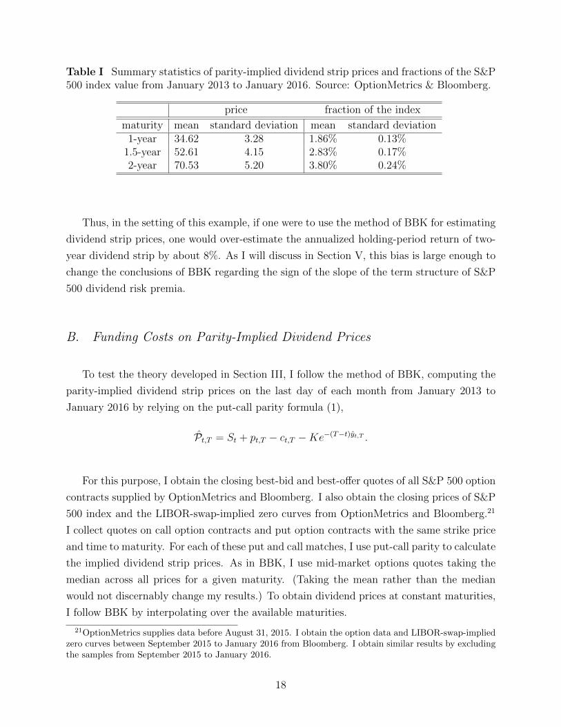
Table I Summary statistics of parity-implied dividend strip prices and fractions of the S&P500 index value from January 2013 to January 2016. Source: OptionMetrics & Bloomberg.

price fraction of the index

maturity mean standard deviation mean standard deviation1-year 34.62 3.28 1.86% 0.13%

1.5-year 52.61 4.15 2.83% 0.17%2-year 70.53 5.20 3.80% 0.24%

Thus, in the setting of this example, if one were to use the method of BBK for estimating

dividend strip prices, one would over-estimate the annualized holding-period return of two-

year dividend strip by about 8%. As I will discuss in Section V, this bias is large enough to

change the conclusions of BBK regarding the sign of the slope of the term structure of S&P

500 dividend risk premia.

B. Funding Costs on Parity-Implied Dividend Prices

To test the theory developed in Section III, I follow the method of BBK, computing the

parity-implied dividend strip prices on the last day of each month from January 2013 to

January 2016 by relying on the put-call parity formula (1),

Pt,T = St + pt,T − ct,T −Ke−(T−t)yt,T .

For this purpose, I obtain the closing best-bid and best-offer quotes of all S&P 500 option

contracts supplied by OptionMetrics and Bloomberg. I also obtain the closing prices of S&P

500 index and the LIBOR-swap-implied zero curves from OptionMetrics and Bloomberg.21

I collect quotes on call option contracts and put option contracts with the same strike price

and time to maturity. For each of these put and call matches, I use put-call parity to calculate

the implied dividend strip prices. As in BBK, I use mid-market options quotes taking the

median across all prices for a given maturity. (Taking the mean rather than the median

would not discernably change my results.) To obtain dividend prices at constant maturities,

I follow BBK by interpolating over the available maturities.

21OptionMetrics supplies data before August 31, 2015. I obtain the option data and LIBOR-swap-impliedzero curves between September 2015 to January 2016 from Bloomberg. I obtain similar results by excludingthe samples from September 2015 to January 2016.

18

Table I presents summary statistics for 1-year, 1.5-year, and 2-year parity-implied syn-

thetic dividend prices from January 2013 to January 2016. The average implied market

values of these synthetic dividend strips, in dollars, are 34.62, 52.61 and 70.53, respectively.

Over the sample period, the parity-implied dividend strip prices are on average 1.86%, 2.83%,

and 3.80% of the S&P 500 index value, respectively. These estimates are similar to those of

BBK over their sample period from 1996 to 2009.

I have shown (see (12)) that the parity-implied dividend strip price Pt,T is negatively

correlated with the funding cost to dealers of hedging inventory, given by Stρt,T (T − t). To

test this, I estimate the following model:

Pt,t+hSt

= α + β(ρt,t+hh) + γTXt + εt+h, (13)

where Pt,t+h is the parity-implied dividend price with maturity h, ρt,t+h is the spread at

maturity h between the S&P 500 repo rate and LIBOR-swap-implied zero rate, and Xt

includes a series of control variables, including the CBOE VIX index, the TED spread,

corporate bond spread, etc. I assume that the residuals εt+h satisfy the standard conditions

for ordinary-least-squares estimation. The interested parameter is β in (13).

There are no reasons to expect that the funding costs to dealers’ shareholders of hedging

S&P 500 index options should have a significant impact on market values of short-term

dividend strips. As a result, if parity-implied dividend prices calculated by the method of

BBK are unbiased, then we should expect to find

β = 0. (14)

I refer equation (14) as the null hypothesis.

Table II reports the regression results. As one can see, the estimate of β is negative

and statistically significant for all the three maturities of 1.5-year, 1.75-year, and 2-year,

corresponding to the maturity specturm of dividend risk premia estimated by BBK. In other

words, we could readily reject the null hypothesis that β = 0. Moreover, the magnitude of

β is economically important. For example, the estimated parameter β in the multi-variate

regression is−1.17 for the 2-year maturity, with a t-statistic of−3.26. This would correspond,

for a spread ρt,t+2 of 32 bps, (the average spread from data reported in Section IV.A,) to

an upward bias in the estimated strip price of around 17%. That is, the cost to dealers of

financing S&P 500 index hedges has a significant impact on parity-implied dividend strip

19

Table II Regression results for (13). The period is from January 2013 through January2016, and the frequency is monthly. TED spread is the difference between 3-month LIBORrate and 3-month T-bill interest rate, VIX is the CBOE volatility index, Three-month LIBORis the 3-month LIBOR rate based on U.S. Dollar, HML and SMB are Fama-French HML andSMB factors, Baa-Fed Funds is Moody’s seasoned Baa corporate bond yield minus federalfunds rate, Term premium is the term premium on 10-year zero coupon U.S. treasury bond.t-statistics are reported in parentheses. ***,**, and * denote statistical significance at the1, 5, and 10% level.

maturity h 1.5-year 1.75-year 2-year(1) (2) (3) (4) (5) (6)

β -0.73** -1.02*** -0.89** -1.15*** -0.98*** -1.17***(-1.97) (-3.17) (-2.48) (-3.23) (-2.72) (-3.26)

TED spread 5.49e-03 9.17e-3 8.04e-3(0.33) (0.49) (0.37)

VIX 4.49e-05 3.89e-5 2.62e-5(0.47) (0.36) (0.21)

Three-month LIBOR -0.025 -0.030 -0.029(-1.22) (-1.27) (-1.07)

HML -1.89e-04 -2.01e-4 -1.92e-4(-1.59) (-1.49) (-1.23)

SMB 5.69e-05 1.37e-4 2.14e-4(0.39) (0.82) (1.11)

Baa-Fed Funds 4.20e-03*** 5.12e-3*** 5.65e-3***(3.01) (3.30) (3.17)

Term premium -5.56e-03*** -6.26e-3*** -6.74e-3***(-3.23) (-3.24) (-3.01)

R-squared 0.11 0.49 0.17 0.54 0.20 0.55

20

prices, in accordance with the predictions of my model of dealer financing.

BBK also highlight the “excess” volatility of their estimated parity-implied dividend strip

prices. The regression (13) shows that a moderately large portion of the variation in the

parity-implied dividend prices can be attributed to funding costs for S&P 500 index hedges.

For example, the reported R2 implies that funding costs along could explain about 20 percent

of the variation (sample variance) in 2-year parity-implied dividend prices over the sample

period.

I also estimate the following regression on innovations of parity-implied dividend prices

and repo spreads:

∆Pt,t+hSt

= α + β(∆ρt,t+hh) + γT∆Xt + εt+h, (15)

where ∆Pt,t+h/St = Pt+δ,t+δ+h/St+δ − Pt,t+h/St, ∆ρt,t+h = ρt+δ,t+δ+h − ρt,t+h, and ∆Xt =

Xt+δ − Xt, with δ = 1/12, corresponding to monthly frequency. Table III reports the

results. Consistent with the model predictions, the estimate of β is negative and statistically

significant at all maturities. None of the control variables is statistically significant. Further,

the variation in parity-implied dividend prices is largely explained by the changes in dealer

funding costs.

To summarize, these simple regressions show that put-call-parity-implied dividend prices

are negatively correlated with the costs to dealers for financing of hedges, consistent with the

predictions of my model in Section III. Although I rely on S&P 500 repo rates observations

and option prices from the post-crisis period, these data are likely to be informative for the

BBK sample period.

V. S&P 500 Dividend Risk Premia: A Second Look

This section provides estimates of the biases in the dividend risk premia reported by

BBK, and presents related evidence from other asset markets.

21

Table III Regression results for (15). The period is from January 2013 through January2016, and the frequency is monthly. TED spread is the difference between 3-month LIBORrate and 3-month T-bill interest rate, VIX is the CBOE volatility index, Three-month LIBORis the 3-month LIBOR rate based on U.S. Dollar, HML and SMB are Fama-French HMLand SMB factors, Baa-Fed Funds is Moody’s seasoned Baa corporate bond minus federalfunds rate, Term premium is the term premium on 10-year zero coupon U.S. treasry bond.t-statistics are reported in parentheses. ***,**, and * denote statistical significance at the1, 5, and 10% level.

maturity h 1.5-year 1.75-year 2-year(1) (2) (3) (4) (5) (6)

β -1.26** -1.20** -1.33*** -1.22*** -1.31*** -1.15***(-2.43) (-2.40) (-2.84) (-2.64) (-2.96) (-2.60)

TED spread 0.023 0.026 0.025(1.23) (1.33) (1.13)

VIX 8.86e-05 1.16e-4 1.47e-4(0.98) (1.21) (1.39)

Three-month LIBOR -0.014 5.88e-3 -0.021(-0.39) (-0.52) (-0.48)

HML 1.24e-04 -1.22e-04 -1.01e-4(-1.46) (-1.12) (-1.01)

SMB -2.15e-04 -1.77e-04 -1.60e-4(-1.45) (-1.24) (-0.91)

Baa-Fed Funds -1.04e-03 -1.02e-03 -1.41e-3(-0.38) (-0.34) (-0.43)

Term premium -1.22e-03 -1.13e-03 -7.12e-4(-0.48) (-0.42) (-0.24)

R-squared 0.16 0.44 0.22 0.47 0.23 0.45

22

A. Dividend Investment Strategies of BBK

Relying on the put-call parity-implied dividend strip prices, BBK calculate the returns

of two hypothetical strategies, which involve investing in S&P 500 dividend strips with

maturities of 1.4 to 1.9 years. BBK report that the two strategies earn returns higher than

that of investing in the S&P 500 index. As a result, BBK claim that the term structure of

the S&P 500 dividend risk premia is on average downward sloping.

In this section, I show that the estimate by BBK of the risk premia for these short-term

S&P 500 dividend strips might be biased upward in a notable way. If this bias is large

enough, which is plausible given the illustrative S&P 500 repo data that I have shown, then

the claim by BBK that the term structure of risk premia for S&P 500 dividends is downward

sloping would not be correct.

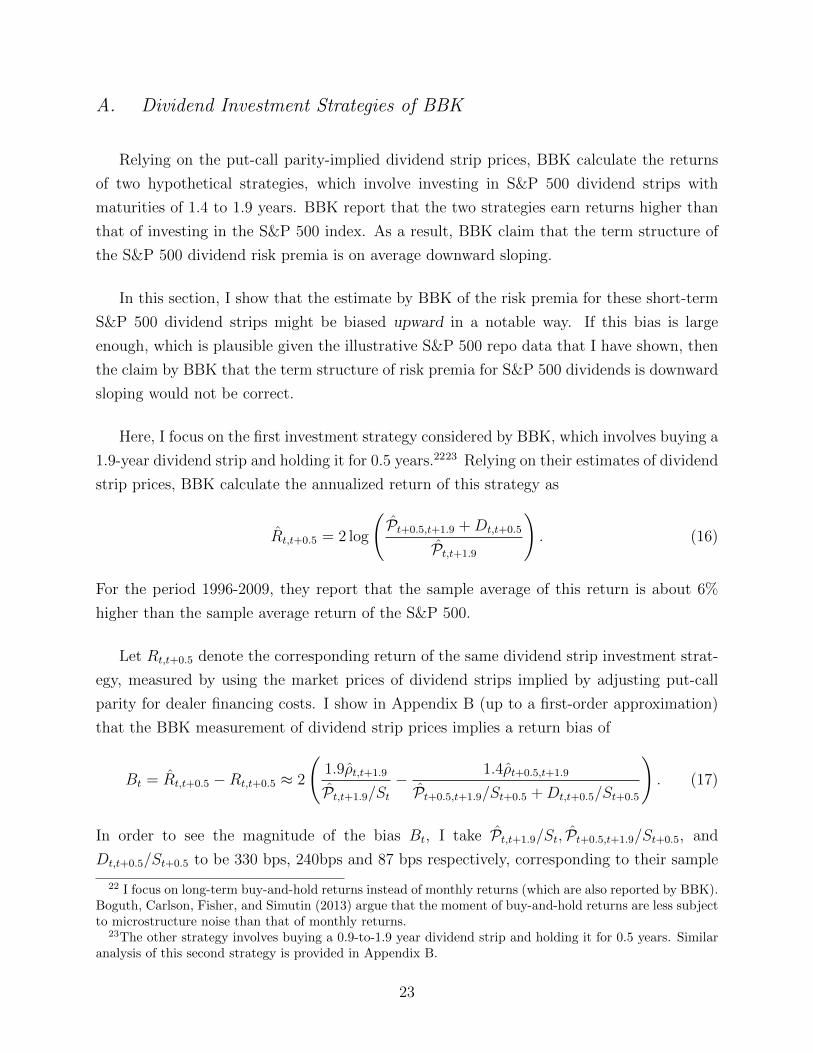
Here, I focus on the first investment strategy considered by BBK, which involves buying a

1.9-year dividend strip and holding it for 0.5 years.2223 Relying on their estimates of dividend

strip prices, BBK calculate the annualized return of this strategy as

Rt,t+0.5 = 2 log

(Pt+0.5,t+1.9 +Dt,t+0.5

Pt,t+1.9

). (16)

For the period 1996-2009, they report that the sample average of this return is about 6%

higher than the sample average return of the S&P 500.

Let Rt,t+0.5 denote the corresponding return of the same dividend strip investment strat-

egy, measured by using the market prices of dividend strips implied by adjusting put-call

parity for dealer financing costs. I show in Appendix B (up to a first-order approximation)

that the BBK measurement of dividend strip prices implies a return bias of

Bt = Rt,t+0.5 −Rt,t+0.5 ≈ 2

(1.9ρt,t+1.9

Pt,t+1.9/St− 1.4ρt+0.5,t+1.9

Pt+0.5,t+1.9/St+0.5 +Dt,t+0.5/St+0.5

). (17)

In order to see the magnitude of the bias Bt, I take Pt,t+1.9/St, Pt+0.5,t+1.9/St+0.5, and

Dt,t+0.5/St+0.5 to be 330 bps, 240bps and 87 bps respectively, corresponding to their sample

22 I focus on long-term buy-and-hold returns instead of monthly returns (which are also reported by BBK).Boguth, Carlson, Fisher, and Simutin (2013) argue that the moment of buy-and-hold returns are less subjectto microstructure noise than that of monthly returns.

23The other strategy involves buying a 0.9-to-1.9 year dividend strip and holding it for 0.5 years. Similaranalysis of this second strategy is provided in Appendix B.

23

averages reported by BBK.24 I assume that the sample average of the repo-to-swap spread

ρt+0.5,t+1.9 is identical to the sample average of ρt,t+1.9 provided in Section IV.B. This is

conservative. The data suggest that the spread between the S&P 500 repo rate and LIBOR-

swap-implied zero rate is higher at longer maturities, as shown in Figure 1.

A 1-basis-point increase in ρt,t+1.9, the spread between S&P 500 repo rate and LIBOR-

swap-implied zero rate, increases the return bias Rt,t+0.5 − Rt,t+0.5 by 27 bps. For a spread

ρt,t+1.9 of 30 bps, the average spread from data reported by a large dealer bank, the implied

return bias Rt,t+0.5−Rt,t+0.5 is around 8%. That is, the high average returns of the investment

strategy considered by BBK might be an artifact of the effect of dealers’ funding costs. The

true risk premia for these short-term S&P 500 dividend strips might be much lower than the

BBK estimate. As a result, the claim by BBK regarding the term structure of risk premia

for S&P 500 dividends, relying on these biased estimates of short-term S&P 500 dividend

risk premia, might not be correct.

B. Evidence from Other Asset Markets

Subsequent work by van Binsbergen, Hueskes, Koijen, and Vrugt (2013) (BHKV), by

van Binsbergen and Koijen (2015) (BK), by Cejnek and Randl (2015) (CR (2015)), and

by Cejnek and Randl (2016)(CR (2016)) rely directly on S&P 500 dividend swap pricing

data,25 and is therefore not subject to the bias that I address in this paper. In any case, this

subsequent work by BHKV (2013), BK (2015), CR (2015) and CR (2016) does not appear

to provide support for the earlier suggestion by BBK (2012) of an average downward sloping

term structure of S&P 500 dividend risk premia.

BHKV (2013) use proprietary S&P 500 dividend swap prices from 2002 to 2011, and

report that, conditionally, the term structure of S&P 500 dividend risk is pro-cyclical. That

is, they suggest that the term structure is upward sloping in normal times and is inverted

during the financial crisis from 2008 to 2009. They also report26 that, unconditionally, the

annualized risk premia for the 1-to-2 year and 4-to-5 year dividend strips are 2.7% and 3.8%

respectively over 2002-2011, while the risk premium of the S&P 500 index is 6.0% over the

24BBK publish their estimates of 6-month, 12-month, 18-month, and 24-month dividend strips prices. Seehttps://www.aeaweb.org/articles.php?doi=10.1257/aer.102.4.1596. Following BBK, I estimate the1.4-year and 1.9-year dividend strips prices by linear interpolation.

25Although standardized OTC dividend swaps and listed futures co-exist for several other indexes, S&P500 has no listed dividend futures contract.

26See Figure 6 of BHKV (2013).

24

same period. These estimates are consistent with a term structure of S&P 500 dividend risk

premia that is upward sloping on average, in contrast with the result suggested by BBK

(2012).

BK (2015) rely on a longer sample of dividend swap prices from 2002 to 2014. They esti-

mate27 that the monthly holding-period returns of 1-year and 1-to-2 year S&P 500 dividend

strips are lower than that of the S&P 500 by 2.76% and 0.24% respectively (on an annualized

basis) over 2002-2014. CR (2015) use a sample of S&P 500 dividend swap prices from 2006

to 2013 and CR (2016) use a sample from 2005 to 2015. They also report that the returns of

1-year to 5-year S&P 500 dividend strategies underperform those of the benchmark index.28

On the hand other, BK (2015) document that short-term dividend strips have outper-

formed their corresponding index in Europe. This study uses the dividend futures prices

rather than put-call parity and options prices. Understanding heterogeneity in the term

structure of equity risk premia across different countries is an important research question

that is beyond the scope of this paper. Relying on dividend futures prices, BK (2015) also

document that the point estimate of short-end equity risk premia is higher than that of the

index premium in Japan and in the UK, but the results are statistically insignificant.

C. Bid-Offer Spreads of Long-Dated Options

I have shown that some supposed “no-arbitrage” pricing relationships frequently break

down due to dealers’ funding costs of carrying and hedging derivatives inventory. A natural

question is whether some sophisticated investors, such as hedge funds or “deep-pocket”

investors, could take advantage of the implied seemingly low-risk “arbitrage” opportunity.

In practice, possibly due to bid-ask spreads, shorting access, and capital-raising frictions,

among other capital market frictions, it may be difficult for investors to take advantage of

the implied opportunities. For example, investors incur options bid-ask spreads in order to

establish the synthetic dividend positions of the BBK strategy.29 The bid-ask spreads for

long-dated options contracts are normally wide. For example, between 2002 to 2007, the

average bid-offer spread for long-dated S&P 500 index options30 with maturities between

27See Table 2 of BK (2015).28See Figure 1 and Table 2 of CR (2015), and Table 1 of CR (2016).29BBK use mid-market options prices.30I collect the daily best-offer and best-bid prices of all the S&P 500 options contracts with a time-to-

25

one year and two years is $2.77. The average estimate by BBK of the 1.5-year synthetic

dividend price is $32.65. This implies a proportional transaction cost of about 8.5%. The

proportional transaction cost of the second BBK investment strategy is even larger because

it involves selling an additional short-term synthetic dividend.

VI. Conclusion

When providing immediacy to ultimate investors, derivatives dealers usually have net

cash funding requirements for hedging their dealing inventories. I show that repo financing of

the hedging positions is generally preferred by a dealer’s shareholders over general unsecured

debt issuance or secondary equity offerings. Under the assumption that dealers maximize

their shareholders’ total equity market value, I show that equilibrium mid-market derivatives

prices depend on the spread between repo rates for the underlying asset and market risk-free

rates.

An implication is that some supposed “no-arbitrage” pricing relationships, which rely on

the notion that any net funding needs are financed at market risk-free rates, frequently break

down. Reliance on standard parity relationships can thus lead to biased results. (Moreover,

as a matter of measurement, since the financial crisis, risk-free rates are no longer well

approximated by LIBOR-swap-implied interest rates.)

As an application, I show that the risk premia for short-term S&P 500 dividends esti-

mated by van Binsbergen, Brandt, and Koijen (2012), which rely on standard put-call parity

to deduce the implied prices of dividend strips, might be notably upward biased. In partic-

ular, I question whether the term structure of S&P 500 dividend risk premia is on average

downward-sloping, as this research suggested.

REFERENCES

Andersen, Leif, Darrell Duffie, and Yang Song, 2016, Funding value adjustment, Working

paper, Stanford University. Available at http://ssrn.com/abstract=2746010.

exercise of between one and two years from OptionMetrics. I exclude contracts with zero open interest. Iexclude prices from 2008 to 2009 to avoid the impact of the financial crisis.

26

Boguth, Oliver, Murray Carlson, Adlai Fisher, and Mikhail Simutin, 2013, Leverage and

the limits of arbitrage pricing: Implications for dividend strips and the term structure of

equity risk premia, Working paper, University of British Columbia.

Brennan, Michael, and Eduardo Schwartz, 1990, Arbitrage in stock index futures, The Jour-

nal of Business 63, 7–31.

Cejnek, Georg, and Otto Randl, 2015, Risk and return of short-duration equity investments,

Working paper, WU Vienna University of Economics and Business.

Cejnek, Georg, and Otto Randl, 2016, Dividend risk premia, Available at http://papers.

ssrn.com/sol3/Papers.cfm?abstract_id=2725073.

Collin-Dufresne, Pierre, and Bruno Solnik, 2001, On the term structure of default premia in

the swap and LIBOR markets, The Journal of Finance 56, 1095–1115.

Combescot, Philippe, 2013, Recent changes in equity financing, Available at https://www.

soa.org/Files/Pd/2013/2013-ga-EBIG-combescot.pdf.

Credit Suisse, 2013, Extracting the dividend risk premium, Available at https:

//edge.credit-suisse.com/Edge/public/bulletin/ServeFile.aspx?FileID=

24848&m=-187350540.

Duffie, Darrell, and Kenneth Singleton, 1997, An econometric model of the term structure

of interest rate swap yields, The Journal of Finance 52, 1287–1323.

Feldhutter, Peter, and David Lando, 2008, Decomposing swap spreads, Journal of Financial

Economics 88, 375–405.

Garleanu, Nicolae, Lasse Pedersen, and Allen Poteshman, 2009, Demand-based option pric-

ing, The Review of Financial Studies 22, 4259–4299.

Hu, Xing, Jun Pan, and Jiang Wang, 2015, Tri-party repo pricing, Working paper, MIT.

Hull, John, and Alan White, 2013, LIBOR vs. OIS: the derivatives discounting dilemma,

Journal of Investment Management 11, 14–27.

Hull, John, and Alan White, 2015, Optimal delta hedging for equity options, Working paper,

University of Toronto.

Lou, Wujiang, 2014, Extending the Black-Scholes option pricing theory to account for an op-

tion market maker’s funding costs, Available at SSRN: http://papers.ssrn.com/sol3/

papers.cfm?abstract_id=2410006.

27

Piterbarg, Vladimir, 2010, Funding beyond discounting: Collateral agreements and deriva-

tives pricing, Risk, February, 97–102.

Roll, Richard, Eduardo Schwartz, and Avanidhar Subrahmanyam, 2007, Liquidity and the

law of one price: The case of the futures-cash basis, The Journal of Finance 62, 2201–2234.

Schulz, Florian, 2015, On the timing and pricing of dividends: Comment, American Eco-

nomic Review, forthcoming.

Skarecky, Tod, 2015, Swap spreads for dummies - the LIBOR joke, Available at

https://www.clarusft.com/swap-spreads-for-dummies-the-libor-joke/?utm_

source=Clarus+Financial+Technology+Newsletter&utm_campaign=6ca3693352-RSS_

EMAIL_CAMPAIGN&utm_medium=email&utm_term=0_09a3151e3a-6ca3693352-79076113.

van Binsbergen, Jules, Michael Brandt, and Ralph Koijen, 2012, On the timing and pricing

of dividends, American Economic Review 102, 1596–1618.

van Binsbergen, Jules, Wouter Hueskes, Ralph Koijen, and Evert Vrugt, 2013, Equity yields,

Journal of Financial Economics 110, 503–519.

van Binsbergen, Jules, and Ralph Koijen, 2015, The term structure of returns: facts and

theory, Working paper, the Wharton school, University of Pennsylvania.

28

Appendix A Proofs and Other Calculations for

Section II

This appendix supplies proofs of Lemmas 1 and 2, and Propositions 1 and 2.

Proof of Lemma 1: Because I have assumed a competitive capital market with complete

information, creditors offering the new debt break even. That is, the market credit spread

s(q) on the new debt, which is issued to finance the hedging position, solves

Y = E

[M1

(1Dc(q)(Y + s(q)) + 1D(q)

κ(A+ q(S1 +D1) + q(S1 − F )−)

L+ qS0(Y + s(q)) + q(S1 − F )+(Y + s(q))

)],

where Dc(q) is the dealer’s survival event {A+q(S1+D1)−q(S1−F )−qS0(Y +s(q))−L > 0}.By letting q go to zero, it is easy to see that limq→ s(q) exists, and

limq→0

s(q) = s =Y 2E[M11D(1− κA/L)]

1− Y E[M11D(1− κA/L)],

where s is the dealer’s original unsecured credit spread.

If the dealer finances the hedging position by issuing new debt, then the marginal value

of the portfolios to its shareholders is

G =∂E[M1(A+ q(S1 +D1)− q(S1 − F )− qS0(Y + s(q))− L)+]

∂q

∣∣∣∣q=0

.

The objective is to show that the derivatives exists and is given by

G = E[M11Dc(F +D1 − S0(Y + s))].

By definition,

G = limq→0

E[M11Dc(q)(A+ q(D1 + F )− L− qS0(Y + s(q)))]− E[M11Dc(A− L)]

q

= limq→0

E[M11Dc(q)(q(D1 + F )− qS0(Y + s(q)))] + E[M1(1Dc(q) − 1Dc)(A− L)]

q.

29

It is easy to see that

limq→0

E[M11Dc(q)(q(D1 + F )− qS0(Y + s(q)))]

q

= limq→0

E[M11Dc(q)(D1 + F − S0(Y + s(q)))]

= E[M11Dc(D1 + F − S0(Y + s))],

where the last equality is due to the fact that A and L have finite expectations, allowing

interchangeability of the limit and expectation.

Notice that

1Dc(q) − 1Dc = 1Dc(q)∩D − 1D(q)∩Dc ,

and

|A− L| ≤ q|D1 + F − (Y + s(q))S0|

in the events Dc(q) ∩ D and D(q) ∩ Dc. Thus,

limq→0

E[M1|(1Dc(q) − 1Dc)(A− L)|]q

≤ limq→0

E[M1|1Dc(q)∩D(A− L)|] + E[M1|1D(q)∩Dc(A− L)|]q

≤ limq→0

E[M1|(1Dc(q)∩D + 1D(q)∩Dc)(D1 + F − S0(Y + s(q)))|].

By the Lebesgue Dominated Converge Theorem,

limq→0

E[M1|(1Dc(q)∩D + 1D(q)∩Dc)(D1 + F )|] = E

[M1 lim

q→0|(1Dc(q)∩D + 1D(q)∩Dc)(D1 + F )|

]= 0,

where the last equality is due to the fact that A and L have a continuous joint density.

Because limq→0 s(q) exist, I also have

limq→0

E[(1Dc(q)∩D + 1D(q)∩Dc)S0(r + s(q))

]= 0.

Thus,

limq→0

E[M1|(1Dc(q) − 1Dc)(A− L)|]q

= 0,

and I have shown that

G = E[M11Dc(F +D1 − S0(Y + s))].

30

Proof of Lemma 2: If the dealer finances the hedging position through the repo market,

then the total equity claim is E[M1(A+q(S1 +D1)−q(S1−F )−qS0Ψ0−L)+], where Ψ0−1

is the underlying repo rate.

Thus, the marginal value of the portfolios to its shareholders is

G =∂E[M1(A+ q(S1 +D1)− q(S1 − F )− qS0Ψ0 − L)+]

∂q

∣∣∣∣q=0

.

Similar calculations from the proof of Lemma 1 apply here, and one can easily show that G

exists and is given by

G = E[M11Dc(F +D1 − S0Ψ0)].

The Case of Equity Financing: I also consider the case that the dealer finances the

hedging positions by issuing new equities. Because the investors in a competitive market for

the newly issued equity break even on the purpose of shares, then the market value of the

legacy shareholders’ equity is given by

E[M1(A+ q(S1 +D1)− q(S1 − F )− L)+]− qS0.

One can show as in the proof of Lemma 1 that the marginal value of the portfolios to

the dealer’s legacy shareholders exists and is given by

G = E[M11Dc(D1 + F )]− S0.

Proof of Proposition 1 : I have assumed that Ψ0 < Y + s. That is, the repo rate of the

underlying is assumed to be lower than the dealer’s unsecured financing rate. Thus, it is

straightforward to see that

G > G.

On the other hand, if the repo rate is higher than the dealer’s unsecured financing rate,

that is, Ψ0 ≥ Y + s, then

G ≤ G.

Now I show that G > G, that is, the marginal value to shareholders under unsecured

31

debt financing is strictly higher than the marginal value under equity financing. It suffices

to show that

E[M11Dc(Y + s)] < 1.

Recall that the dealer’s unsecured credit spread

s =Y 2E[M11D(1− κA/L)]

1− Y E[M11D(1− κA/L)].

Thus, I only need to show

Y (E[M11Dc ] + E[M11D(1− κA/L)]) < 1.

This is an immediate result due to 1D(1− κA/L) < 1D and Y E(M1) = 1.

The Case of Bid Quotes: If an end user wants to sell a forward position, a dealer usually

hedges its position through reverse repo in the repo market. That is, in the opening leg, the

dealer receives the underlying and supplies cash to the repo counterparty, where the cash is

from selling the underlying. In the closing leg, the dealer buys back underlying and return

the underlying, together with dividend, in exchange for cash and interest rate, which is the

repo rate.

In this case, the total equity claim to the dealer’s shareholder is

(A+ qS0Ψ0 + q(S1 − F )− q(S1 +D1)− L)+.

Following similar calculations as in the proof of Lemma 1, the marginal value of the net

trade to shareholders is

E[M11Dc(S0Ψ0 − F −D1)].

Proof of Proposition 2 : I have assumed that dealers maximize their shareholders values.

In a competitive bidding upon the request from an end user, dealers choose to finance the

hedging positions in the repo market. As a result, the equilibrium forward offer and bid

prices are identical, given by

F = S0Ψ0 −E(M11DcD1)

E(M11Dc).

32

Appendix B Calculations for Section V

Derivation of (17):

Rt,t+0.5 = 2 log

(Pt+0.5,t+1.9 +Dt,t+0.5

Pt,t+1.9

)≈ 2 log

(Pt+0.5,t+1.9 + 1.4St+0.5ρt+0.5,t+1.9 +Dt,t+0.5

Pt,t+1.9 + 1.9Stρt,t+1.9

),

where we recall from (12) that

Pt,T ≈ Pt,T − Stρt,T (T − t).

Thus,

Bt = (Rt,t+0.5 −Rt,t+0.5)

= 2 log

(1 +

1.9ρt,t+1.9

Pt,t+1.9/St

)− 2 log

(1 +

1.4ρt+0.5,t+1.9

Pt+0.5,t+1.9/St+0.5 +Dt,t+0.5/St+0.5

)

≈ 2

(1.9ρt,t+1.9

Pt,t+1.9/St− 1.4ρt+0.5,t+1.9

Pt+0.5,t+1.9/St+0.5 +Dt,t+0.5/St+0.5

),

where I have used the first-order Taylor expansion.

The Second Dividend Strategy of BBK: The second investment strategy of BBK in-

volves buying a 0.9-to-1.9 year dividend strip and holding it for 0.5-years. BBK rely on

parity-implied dividend prices and calculate the annualized return of this strategy as

rt,t+0.5 = 2 log

(Pt+0.5,t+1.9 − Pt+0.5,t+0.9

Pt,t+1.9 − Pt,t+0.9

).

For the period 1996-2009, BBK report that the sample average of this return is about 3%

higher than the sample average return of the S&P 500.

Let rt,t+0.5 denote the corresponding return of this investment strategy, measured by using

the market prices of dividend strips implied by adjusting put-call parity for dealer financing

33

costs. Thus, the result bias is

Bt ≡ (rt,t+0.5 − rt,t+0.5)

≈ 2 log

(1 +

1.9ρt,t+1.9 − 0.9ρt,t+0.9

(Pt,t+1.9 − Pt,t+0.5)/St

)− 2 log

(1 +

1.4ρt+0.5,t+1.9 − 0.4ρt+0.5,t+0.9

(Pt+0.5,t+1.9 − Pt+0.5,t+0.9)/St+0.5

)

≈ 2

(1.9ρt,t+1.9 − 0.9ρt,t+0.9

(Pt,t+1.9 − Pt,t+0.9)/St− 1.4ρt+0.5,t+1.9 − 0.4ρt+0.5,t+0.9

(Pt+0.5,t+1.9 − Pt+0.5,t+0.9)/St+0.5

).

To see the magnitude of Bt, I take (Pt,t+1.9−Pt,t+0.9)/St and (Pt+0.5,t+1.9−Pt+0.5,t+0.9)/St+0.5

to be the sample averages of 165 bps and 169 bps, reported by BBK. I assume that the sam-

ple averages of the repo-to-swap spreads are identical to the sample averages provided in

Section IV.B. The bias is thus Bt = (rt,t+0.5 − rt,t+0.5) ≈ 5%.

34