CS2012: An introduction to Algorithms and Data Structures

David Rydeheard

Room 2.115

david@cs.man.ac.uk

AND

Graham Gough

Room 2.105

graham@cs.man.ac.uk

1

Module Overview

Aims

This course is an introduction to the design, analysis and wide

variety of algorithms (a topic often called ‘Algorithmics’).

We shall look at the specification of computational tasks, varieties

of algorithms for tasks, demonstrating (through informal proof)

that algorithms perform given tasks, the structure of algorithms

and, finally, measures for comparing the performance of algorithms.

We also consider the implementation of algorithms and relevant

data and program structures, and principles of program design.

2

Contents

1. Idea of Algorithms: algorithms and programs. Some history.

Formalising algorithms, programming languages and machine

models.

2. Specification and correctness. Informal correctness proofs.

3. Performance of algorithms. The issues. Performance measures.

Complexity: Counting, worst- best- and average-cases.

Recurrence relations for computing complexity. Asymptotic

approximation.

4. Searching and sorting algorithms.

5. Trees and graphs and associated algorithms.

6. Hashing

3

Organisation

The module is in two sections. Section (1) is taught by David

Rydeheard; Section (2) by Graham Gough.

The website

All students should consult the website for this module. It contains

(1) all the lecture notes and slides, (2) relevant code, (3) details of

module organisation, (4) useful links to many other relevant sites.

4

Books

The course textbook is:

Mark Allen Weiss, Data Structures. Problem Solving using

JAVA (ISBN 0-201-74835-5) Addison-Wesley. 2001.

This is a high quality book in the area. The lectured material is

based on this textbook. You are all recommended to get access to

it.

Background Reading: Good support textbooks are:

• SEDGEWICK, R. Algorithms in C (ISBN 0-201-51425-7)

Addison-Wesley 1990. A general, good quality, book on

algorithms, with very good detail.

• CORMEN, T. H. et al, Introduction to Algorithms, (ISBN

0-262-530-910) MIT Press 1994. This is an encyclopaedic

reference, well written and extremely thorough.

5

• HAREL, D. Algorithmics; the Spirit of Computing 2nd

Edition, Addison Wesley 1992. A good informal (and readable)

introduction to the subject.

You are also urged to consult some of the classic texts in the area,

chief of which is: Knuth, D. E. Fundamental Algorithms, Addison

Wesley 1968.

6

Algorithms

• What are they? Not really a defined idea. Informally, a recipe,

or procedure, or construction; algorithms themselves consist of

precise descriptions of procedures.

• The word: It’s history lies in Arabicized Persian, from

al-Kuwarizmi (‘the man from Kuwarizm’ - modern-day Khiva),

the mathematician Abu Ja’far Muhammad ibn Musa.

The European translation of his works introduced the

Hindu-Arabic notation for numbers. This is our standard

notation for numbers 120.4 means 1 hundred, 2 tens and 0

units and 4 tenths! It is positional (Hindu) and has a zero

(Arabic). The advantage of this notation is the ease with which

we can express arithmetic algorithms.

7

Complexity of Algorithms (Chapter 5 of textbook)

Idea: We want to compare the performance of different algorithms

for a given task in terms of some measure of efficiency.

For example: We may want to find ‘how long an algorithm

(coded as a program) takes to compute a result’.

But: This varies with (1) program code, (2) programming

language, (3) compiler, (4) processor etc (operating system,

weather...). Time itself is not a useful measure.

We seek: Measures that are intrinsic to an algorithm (ie

independent of all the conditions above), but nevertheless give a

real assessment of the performance of algorithms.

8

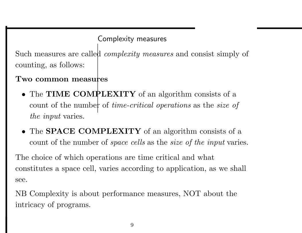
Complexity measures

Such measures are called complexity measures and consist simply of

counting, as follows:

Two common measures

• The TIME COMPLEXITY of an algorithm consists of a

count of the number of time-critical operations as the size of

the input varies.

• The SPACE COMPLEXITY of an algorithm consists of a

count of the number of space cells as the size of the input varies.

The choice of which operations are time critical and what

constitutes a space cell, varies according to application, as we shall

see.

NB Complexity is about performance measures, NOT about the

intricacy of programs.

9

Worst-case, best-case and ‘average-case’ measures

Suppose we are given an algorithm and we wish to assess its

performance on inputs of size N . Usually, even with inputs of a

fixed size, the performance can vary considerably according to the

contents of the input and the arrangement of data.

However, we can identify:

• The best-case performance for each size N - the smallest time

complexity (or space complexity) over all inputs of size N .

• The worst-case performance for each size N - the largest time

complexity (or space complexity) over all inputs of size N .

These are extremal measures, and we would like to be able to

assess the performance on average, but this is more difficult to

compute as we shall see.

10

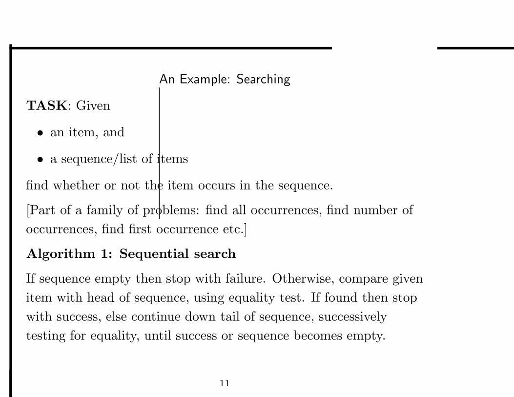
An Example: Searching

TASK: Given

• an item, and

• a sequence/list of items

find whether or not the item occurs in the sequence.

[Part of a family of problems: find all occurrences, find number of

occurrences, find first occurrence etc.]

Algorithm 1: Sequential search

If sequence empty then stop with failure. Otherwise, compare given

item with head of sequence, using equality test. If found then stop

with success, else continue down tail of sequence, successively

testing for equality, until success or sequence becomes empty.

11

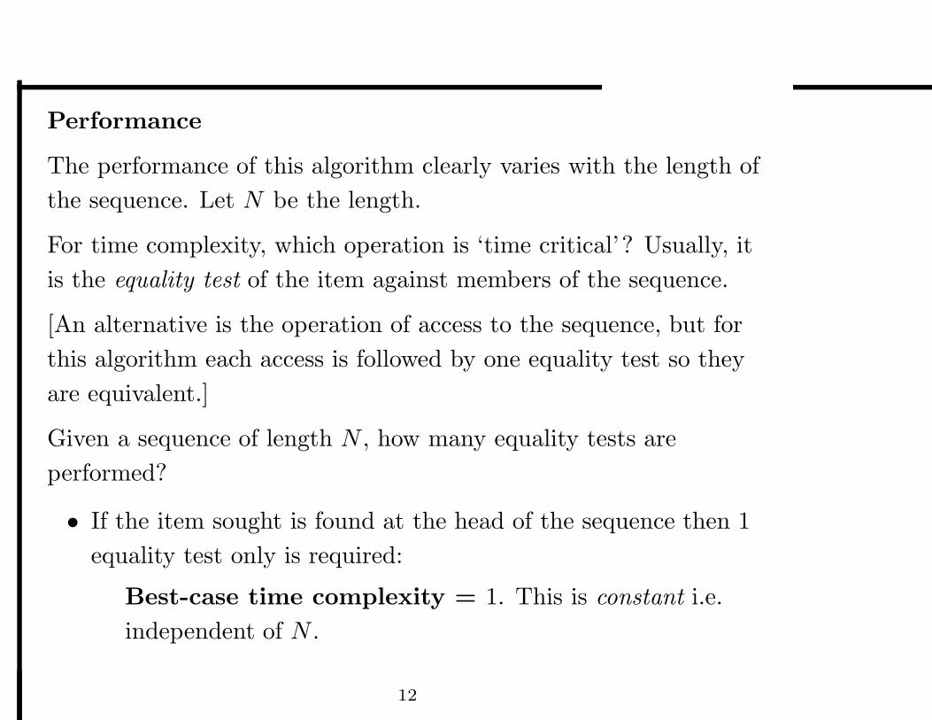
Performance

The performance of this algorithm clearly varies with the length of

the sequence. Let N be the length.

For time complexity, which operation is ‘time critical’? Usually, it

is the equality test of the item against members of the sequence.

[An alternative is the operation of access to the sequence, but for

this algorithm each access is followed by one equality test so they

are equivalent.]

Given a sequence of length N , how many equality tests are

performed?

• If the item sought is found at the head of the sequence then 1

equality test only is required:

Best-case time complexity = 1. This is constant i.e.

independent of N .

12

• If the item sought is found at the end of the sequence or is not

in the sequence then N equality tests are required:

Worst-case time complexity = N . This is linear.

The best-case is the lower bound and the worst case is the upper

bound of any actual performance.

13

‘Average-case’ time complexity

Is either of these - the best-case or the worst-case - a realistic

measure of what happens on average?

Let us try to define average-case time complexity.

This is a difficult concept and often difficult to compute. It involves

probability and infinite distributions.

What is an average sequence of integers? If all integers are equally

probable in the sequence then the probability that any given

integer is in the sequence is zero! (Probability zero does not mean

impossible when there are infinite distributions around.)

14

For sequential search on sequences of random integers this means

Average-case time complexity = N . This is linear and

the same as worst-case.

Note: The average case is NOT the average of the best-case and

worst-case, but is an average over all possible input sequences and

their probabilities of occurrence.

————-

If the sought item is known to occur exactly once in the sequence

and we seek its position, then the average case is N/2.

15

Algorithm 2: Binary Search (Chapter 7 of textbook)

Suppose the items in the sequence are integers - or any type with a

given (total) order relation ≤ on it - and the sequence is already in

ascending (i.e. non-descending) order. Binary search is:

1. If the sequence is empty, return false.

2. If the sequence contains just one item, then return the result of

the equality test.

3. Otherwise: compare given item with a ‘middle’ item:

• If equal, then return success.

• If given item is less than middle item, then recursively call

binary search on the sequence of items to the left of the

chosen middle item.

• If given item is greater than middle item, then recursively

call binary search on the sequence of items to the right of

the chosen middle item.

16

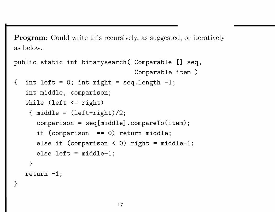
Program: Could write this recursively, as suggested, or iteratively

as below.

public static int binarysearch( Comparable [] seq,

Comparable item )

{ int left = 0; int right = seq.length -1;

int middle, comparison;

while (left <= right)

{ middle = (left+right)/2;

comparison = seq[middle].compareTo(item);

if (comparison == 0) return middle;

else if (comparison < 0) right = middle-1;

else left = middle+1;

}

return -1;

}

17

Note

• The use of Comparable class and compareTo method to

capture the genericity of the algorithm. The comparison here is

a three way comparison, including equality, but other forms are

possible. The algorithm returns either −1 for false, or the

position of the first found occurrence.

• The need for arrays, rather than, say linked lists, because we

need ‘random access’ i.e. access to all parts (esp middle item)

in constant-time. Compare sequential search where either

arrays or linked lists would be appropriate.

18

Correctness of binary search

The argument for the correctness of the algorithm goes as follows:

Suppose we seek an item in a sequence of length N . We proceed by

induction on N .

If N = 0 then the algorithm returns −1 (false) as required.

Otherwise, suppose the algorithm is correct on all ascending

sequences of length less than N . If we can show it is correct on all

ascending sequences of length N , then by induction, it is correct for

all finite ascending sequences.

On an ascending sequence of length N , it first selects an item (the

‘middle’ item) and compares it with the given item, if equal it

returns the position, as required.

If not equal, then because the sequence is in ascending order, if the

item sought is less than the middle item, then it can only occur in

the left subsequence, which itself is an ascending subsequence, but

19

of length at least 1 less than N , so by induction it will correctly

find the item, or return false. Similarly, for the case when the item

is greater than the middle item.

————————

Induction is a characteristic method for iterative and recursive

algorithms as it allows us to establish that something holds

assuming that the remaining part of the computation - the recursive

call, or remaining loop computation - is correct.

Notice that correctness depends upon the ascending order, but

NOT on which element is chosen as the ‘middle’ element (in fact

any element would do for correctness).

20

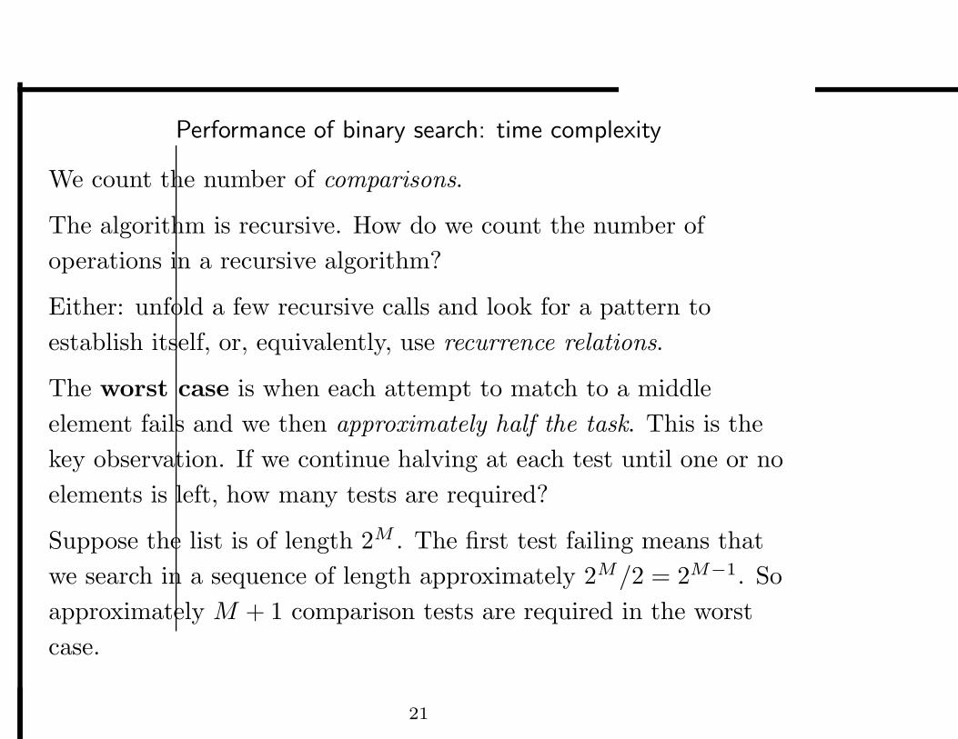
Performance of binary search: time complexity

We count the number of comparisons.

The algorithm is recursive. How do we count the number of

operations in a recursive algorithm?

Either: unfold a few recursive calls and look for a pattern to

establish itself, or, equivalently, use recurrence relations.

The worst case is when each attempt to match to a middle

element fails and we then approximately half the task. This is the

key observation. If we continue halving at each test until one or no

elements is left, how many tests are required?

Suppose the list is of length 2M . The first test failing means that

we search in a sequence of length approximately 2M/2 = 2M−1. So

approximately M + 1 comparison tests are required in the worst

case.

21

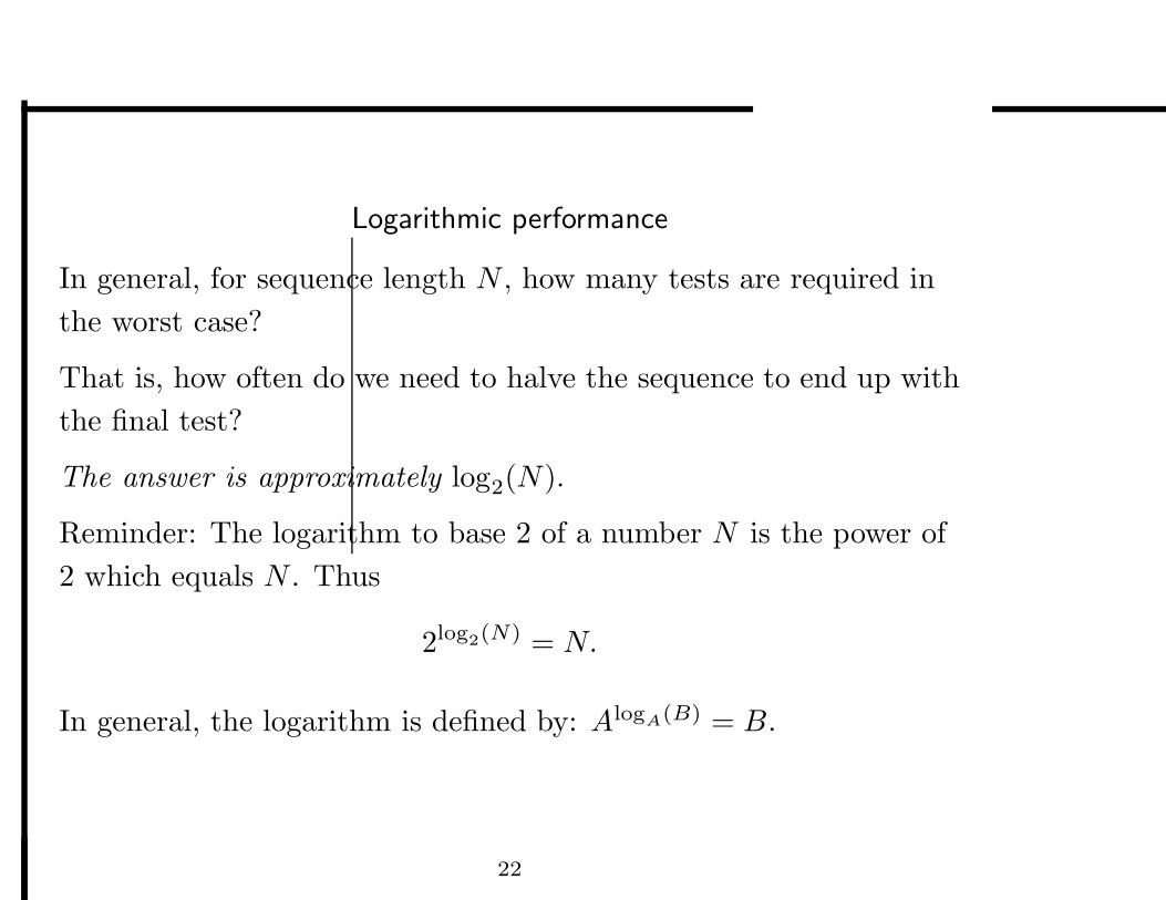
Logarithmic performance

In general, for sequence length N , how many tests are required in

the worst case?

That is, how often do we need to halve the sequence to end up with

the final test?

The answer is approximately log2(N).

Reminder: The logarithm to base 2 of a number N is the power of

2 which equals N . Thus

2log2(N) = N.

In general, the logarithm is defined by: AlogA

(B) = B.

22

Arithmetic with logarithms

The following rules hold for logarithms (all direct from the

definition):

logA(A) = 1, logA(B × C) = logA(B) + logA(C)

logA(1/B) = − logA(B), logB(C) = logB(A) × logA(C).

The second rule above is that for which logarithms were developed

- doing multiplication by addition. The final rule allows us to

change base of logarithms by multiplying by a constant.

23

Logarithms (continued)

Logarithms grow much, much slower that linear - so an algorithm

that performs logarithmically is, in general, very fast:

Linear performance: If the input size doubles, the complexity

doubles.

Logarithmic performance: If the input size doubles, the

complexity increases by 1!

Other common measures are quadratic N 2, and exponential 2N .

24

Input size Logarithmic Linear Quadratic Exponential

10 4 10 100 1024

20 5 20 400 106

100 7 100 10,000 1030

1,000 10 1000 1,000,000 10300

10,000 14 10,000 100,000,00 103000

Thus binary search is very efficient even in the worst case (we can

picture this by saying that half of the material is disposed at each

test without looking at it).

It is also very space efficient. It can be implemented in-place -

without the need for space in addition to that occupied by the

input. However, it does need the input to be in ascending order.

25

Recurrence relations (Chapter 7 of textbook)

... are a general method of calculating the complexity of recursive

and iterative algorithms.

As an example, consider binary search. We introduce the notation

that CN is the number of comparison operations on input of size N

in the worst case.

How do we calculate CN?

26

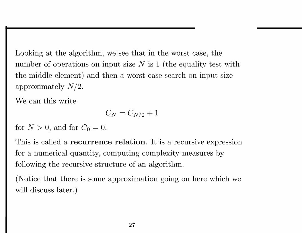
Looking at the algorithm, we see that in the worst case, the

number of operations on input size N is 1 (the equality test with

the middle element) and then a worst case search on input size

approximately N/2.

We can this write

CN = CN/2 + 1

for N > 0, and for C0 = 0.

This is called a recurrence relation. It is a recursive expression

for a numerical quantity, computing complexity measures by

following the recursive structure of an algorithm.

(Notice that there is some approximation going on here which we

will discuss later.)

27

Recurrence relations have solutions.

Sometimes more than one, sometimes one, sometimes none. The

cases we deal with derived for computing the complexity of

algorithms have unique solutions (or a unique family of solutions).

The solution of the above recurrence relation is

CN = log2(N) + 1.

We can see this simply by substituting:

Left-hand side is log2(N) + 1.

Right-hand side is CN/2 + 1 = (log2(N/2) + 1) + 1 =

log2(N × 1/2) + 1 + 1 = log2(N) + log2(1/2) + 1 + 1 =

log2(N) − log2(2) + 1 + 1 = log2(N) − 1 + 1 + 1 = log2(N) + 1.

Hence left-hand and right-hand sides are equal, as required.

(Note: in fact, log2(N) + A for any constant A is a solution, but

base cases determine that A = 1).

28

Finding solutions

Given a solution, we can check it. But our task is to find solutions

of recurrence relations. How do we do this?

A simple approach is to expand the recurrence and see what

happens:

CN = CN/2 + 1 = (CN/4 + 1) + 1 = ((CN/8 + 1) + 1) + 1 = · · · =

C1 + 1 + 1 + · · · + 1

where there are log2(N) number of 1’s. Hence CN = log2(N) + 1 as

required.

In general, algorithms which halve the input at each step have

complexity in terms of logarithms base 2 (if a third at each step

then log base 3 etc).

Later we look at a range of commonly occurring recurrence

relations and we give their solutions.

29

Algorithm complexity: Approximation and rates of growth

In the above analysis we have used approximations: Saying ‘divided

approximately in half’ and even using log2(N) (which in general is

not an integer), rather than ceiling(log2(N)) (the least integer

above log2(N).

Why is this?

It is because we are usually only concerned with the rate of growth

of the complexity as the input size increases.

Complexity (that is the number of operations undertaken) at a

fixed size of input, does NOT in general convert to a running time

for an algorithm. However, if the operations are chosen correctly,

then the rate of growth of the complexity WILL correspond to the

rate of growth of the running time.

30

Rate of growth of numerical expressions

• For complexity log2(N) + 1 is the 1 significant? No. Whatever

the constant is, if the input size doubles the complexity

increases by 1.

For small N , the constant is a significant part of the

complexity, so that log2(N) + 1 and log2(N) + 10 are different,

but as N increases the constant looses its significance.

• For complexity N2 + 1000 ×N + 123456 as N increases so does

the role of the N2 part, and the expression grows like N 2 for

large N .

• For N + 1000 × log2(N) only the linear term N is significant

for large N .

31

In general, for ‘small’ N the behaviour of an algorithm may be

erratic, involving overheads of setting up data structures,

initialization, small components of the complexity, different

operations may be important, etc.

We are interested in the rate of growth of expressions as N

increases, i.e. what happens at ‘large’ N?

32

When N doubles:

• log2(N) increases by 1

• 123 × N doubles

• 12 × N2 quadruples (×4)

• 2 × N3 increases eightfold

• 2N squares (because 22×N = (2N )2)

Exponential algorithms are infeasible - they cannot be run on

substantial inputs to provide results. Note: Exponential includes

factorial N !

33

When N doubles, what happens to N 2 + 1000 × N + 123456?

For ‘small’ N it is approximately constant (because 123456 is big!).

For ‘intermediate’ N it is linear (because 1000 × N dominates over

N2)

But eventually N2 dominates the other terms and the behaviour

becomes closer to quadratic as N increases.

We introduce a notation for this and say that

N2 + 1000 × N + 123456

is O(N2) (Oh, not zero!) and read this as the expression is of

order N2. This is called BIG-OH notation.

34

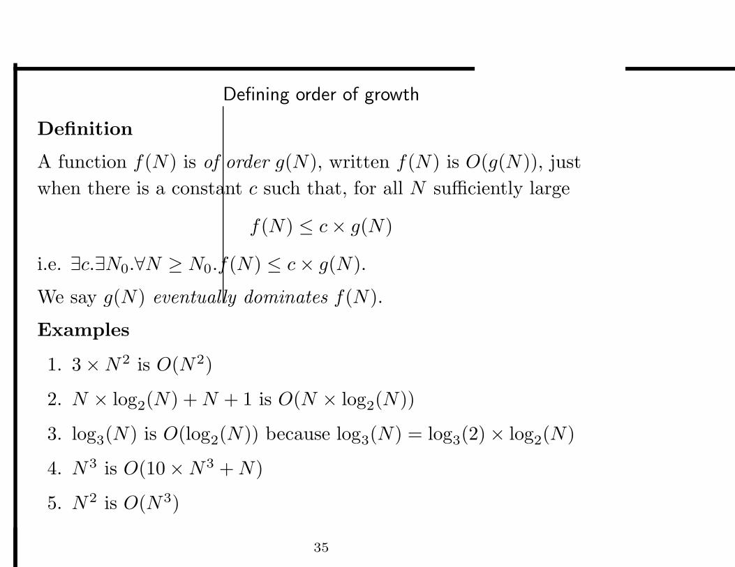
Defining order of growth

Definition

A function f(N) is of order g(N), written f(N) is O(g(N)), just

when there is a constant c such that, for all N sufficiently large

f(N) ≤ c × g(N)

i.e. ∃c.∃N0.∀N ≥ N0.f(N) ≤ c × g(N).

We say g(N) eventually dominates f(N).

Examples

1. 3 × N2 is O(N2)

2. N × log2(N) + N + 1 is O(N × log2(N))

3. log3(N) is O(log2(N)) because log3(N) = log3(2) × log2(N)

4. N3 is O(10 × N3 + N)

5. N2 is O(N3)

35

Recurrence relations and their solutions

Some recurrence relations

• CN = CN/2 + a where a is a constant.

‘Do constant amount of work and then halve the remainder’

Solution: CN = O(log N).

• CN = CN−1 + a where a is a constant.

‘Do constant amount of work and then repeat on input of size

one less’

Typically, this is a simple loop with a constant amount of work

per execution. Example: sequential search.

Solution: CN = O(N).

• CN = CN−1 + a × N where a is a constant.

‘Do amount of work proportional to N and then repeat on

input of size one less’

36

Typically, two nested loops.

CN = CN−1 + a × N = CN−2 + a × (N − 1) + a × N =

CN−3 + a × ((N − 2) + (N − 1) + N) = a × N×(N+1)2

Solution: CN = O(N2) is quadratic.

Examples: Long multiplication of integers, Bubblesort.

• CN = 2 × CN/2 + a × N where a is a constant.

‘Do work proportional to N then call on both halves of the

input’

[Picture]

Solution: CN = O(N × log N). This is called LinLog behaviour

(linear-logarithmic).

• CN = CN−1 + a × N2 where a is a constant.

‘Do amount of work proportional to N 2 and then repeat on

input of size one less’

Typically, three nested loops.

37

Solution: CN = O(N3) is cubic.

Example: The standard method of matrix multiplication.

• CN = 2 × CN−1 + a where a is a constant.

‘Do constant amount of work and then repeat on two versions

of input of size one less’

Solution: CN = O(2N ) - exponential.

• CN = N × CN−1 + a where a is a constant.

Solution: CN = O(N !) = O(NN ) - highly exponential.

(Note: Stirling’s approximation N ! ≈√

2πN(N/e)N .)

38

Infeasible Algorithms

Algorithms with complexities

O(1), O(N), O(N2), O(N3), O(N4) . . .

and between are called polynomial, and are considered as feasible

- ie can be run on ‘large’ inputs (though, of course, cubic, quartic

etc can be very slow).

Exponential algorithms are called infeasible and take

considerable computational resources even for small inputs (and on

large inputs can often exceed the capacity of the known universe!).

39

Examples of Infeasible Algorithms

... are often based on unbounded exhaustive backtracking to

perform an exhaustive search.

Backtracking is ‘trial-and-error’: making decisions until

it is clear that a solution is not possible, then undoing

previous decisions, to try another route to reach a solution.

Unbounded means that we cannot fix how far back we

may need to undo decisions.

The decisions generate a tree and exhaustive search means

traversing this tree to visit all the nodes.

40

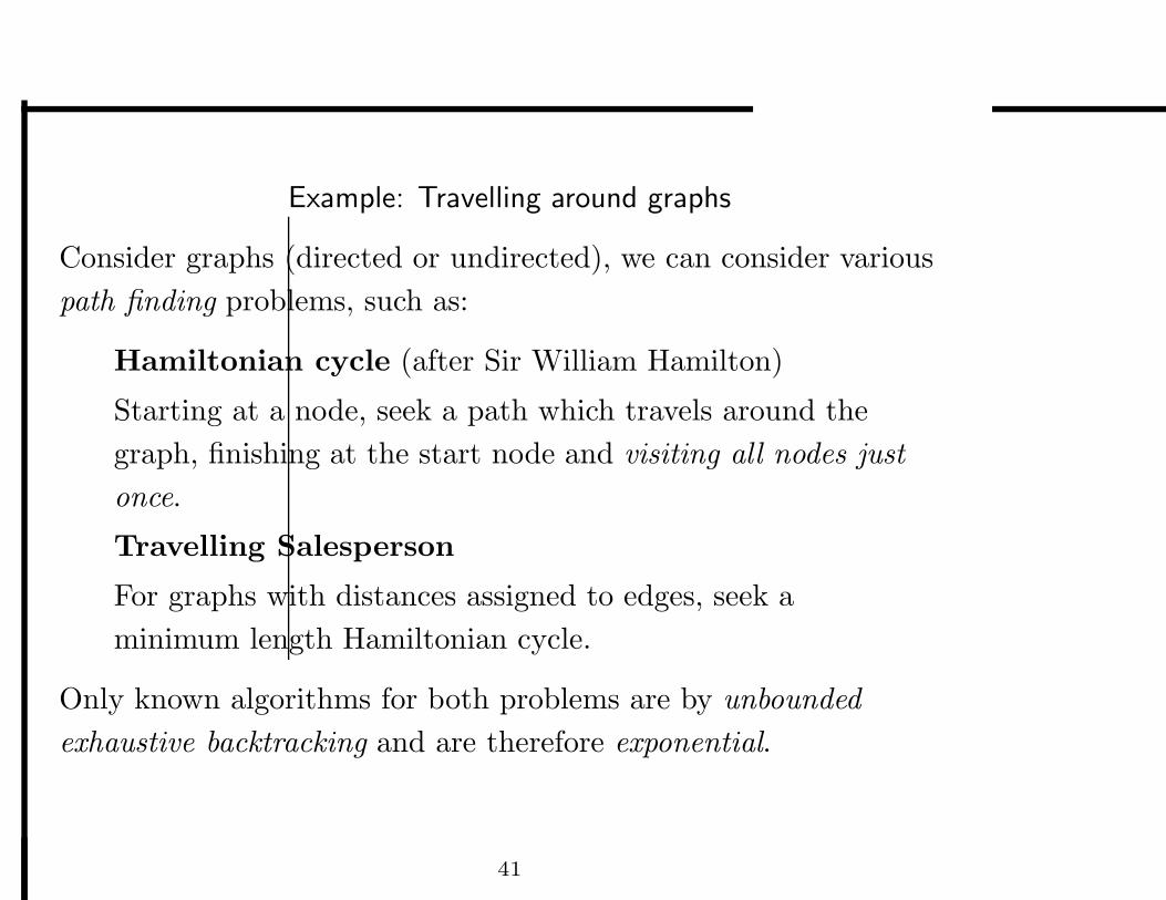
Example: Travelling around graphs

Consider graphs (directed or undirected), we can consider various

path finding problems, such as:

Hamiltonian cycle (after Sir William Hamilton)

Starting at a node, seek a path which travels around the

graph, finishing at the start node and visiting all nodes just

once.

Travelling Salesperson

For graphs with distances assigned to edges, seek a

minimum length Hamiltonian cycle.

Only known algorithms for both problems are by unbounded

exhaustive backtracking and are therefore exponential.

41

Why exponential?

CN = N × CN−1 + a

because, in the worst case, we make one of N initial choices (the

first node visited) and then have a problem of size N − 1, the

choice requires a computation of fixed amount a.

The solution is CN = O(N !) = O(NN ).

42

Other examples: Knapsack problems, games and puzzles

Given an empty box of fixed dimensions, and a number of blocks of

various dimensions:

The task is to choose some of the blocks and arrange them in the

box so that they occupy a maximum amount of space i.e. the empty

(unused) space is minimized.

Algorithms are by exhaustive search.

43

Other examples: Games and puzzles

Many games and puzzles have only infeasible algorithms. That is

what makes them interesting. Compare noughts-and-crosses, which

has a simple algorithm.

For example, the Polyominos puzzle:

Given a range of pieces, of polyomino shape (ie consisting of

squares of constant size fixed together orthogonally, choose some

and fit them onto a chessboard to cover all squares exactly (or on

any other fixed shape board).

44

Complexity theory

Question: Given a computational task, what performance of

algorithms can we expect for it?

Two approaches:

• Invent a range of ‘good’ algorithms.

• Look at the nature of the task and try to determine what range

of algorithms can exist.

Example: Matrix multiplication

The standard algorithm for multiplication of two N ×N matrices is

(obviously) O(N3). For a long while, this was believed to be the

best possible but...

Strassen’s algorithm (1968) is O(N 2.81...)!! and slightly better ones

have been devised since (i.e. slightly smaller exponents).

How good can we get? We simply don’t know.

45

There is an obvious lower bound (minimum number of

operations) of

O(N2)

(because there are N2 results each needing at least one arithmetic

operation).

But what happens between these two?

There is a computational gap between known lower bounds and

known algorithms.

46

Example: Sorting

The task of sorting is to rearrange a list (of integers, say) into

ascending order.

We shall see later that there are algorithms with worst-case time

complexity O(N × log(N)) for this task.

Moreover this is a lower bound: we can show that any general

sorting algorithm must be at least O(N × log(N)).

There is no computational gap.

47

Famous unsolved problem

The examples of tasks which appear to have only exhaustive search

algorithms (travelling salesperson, knapsack etc) are believed to be

intrinsically exponential (ie there are no faster algorithms).

This is the essence of the famous

P 6= NP

conjecture in complexity theory.

(P stands for polynomial - those problems which have polynomial

algorithms, and NP stands for non-deterministic polynomial, and is

the class of problems including travelling salesperson, knapsack

problems etc.)

48