Database-assisted end-to-end theoretical andsimulation framework for cognitive radio

networks

A Dissertation Presentedby

Abdulla K. Al-Alito

The Department of Electrical and Computer Engineeringin partial fulfilment of the requirements

for the degree ofDoctor of Philosophy

inComputer EngineeringNortheastern University

Boston, Massachusetts

April 1, 2014

Abstract

Cognitive radios are envisaged to address the problem of spectrum scarcity by oppor-tunistically using licensed bands, without interfering with the higher priority transmis-sions in them. Recent FCC rulings mandate the use of spectrum databases for obtainingthe spectrum usage information, and how to integrate the database coordination with thehigher layer networking protocol stack remains an open challenge. This dissertation ad-dresses this concern through the following contributions: (a) An end-to-end transport layercalled TFRC-CR is devised that uses equation based transmission rate control, and relieson database updates rather than intermediate node information. (b) A framework for ve-hicular cognitive radio is created that uses cross-correlation between 2G signals obtainedfrom an Android device and signals from the TV white space to reduce the number ofdatabase queries. Moreover, this framework also involves a practical demonstration ofinterference alignment to optimally use the channel during the querying process. (c) Anextension for the network simulator-3 that provides cognitive abilities, such as spectrumsensing, primary user detection, and spectrum hand-off to the research community whichallows them to simulate these complex radios in a virtual environment.

Dedication

This thesis is dedicated to my wife, Marie. Thank you for your support and patience.For your insights and influence that paved the way for me to see and be; to see difficultyas ease, and to be who I am today.

1

Acknowledgements

I want to express my sincere gratitude and appreciation to my mentor and advisor,Dr. Kaushik Chowdhury, for his advice, courage and guidance in my research and for hissupport through the bad and good times. I know I would not be where I am without hishelp and continuous mentoring. I have learned a great deal working under his supervision,and for that will be eternally grateful.

To my family, who, even being so far away for so long, continue to provide their loveand support. To my father and mother; you have always been a role model to me. A rolemodel not just for my career but for the way you show and communicate your enormouscapacity of love.

My lab mates; Rahman, Farima, Prusayon, Yousuf, Yufuk, Meenu, Bruna, Yifan andJinghzi. Your assistance and friendship has meant more than what I can express. Thanksfor all the discussions, help and fun time we had in the lab. I know I will miss that.

And finally, I owe a debt of gratitude to Qatar University, for their continuous supportthroughout my graduate career.

2

Contents

1 Introduction 81.1 Cognitive radio, the motivation and definition . . . . . . . . . . . . . . . 8

1.1.1 Cognitive Radio . . . . . . . . . . . . . . . . . . . . . . . . . . 91.2 Main contributions of this thesis . . . . . . . . . . . . . . . . . . . . . . 101.3 Cognitive radio transport layer design . . . . . . . . . . . . . . . . . . . 111.4 Improve sensing accuracy and optimize the database access policy . . . . 12

1.4.1 Interference temperature . . . . . . . . . . . . . . . . . . . . . . 121.4.2 Local and cooperative spectrum sensing . . . . . . . . . . . . . . 131.4.3 The FCC database . . . . . . . . . . . . . . . . . . . . . . . . . 14

1.5 A cognitive radio module for the network simulator 3 . . . . . . . . . . . 18

2 Cognitive radio transport layer design 202.1 Problem overview . . . . . . . . . . . . . . . . . . . . . . . . . . . . . . 202.2 Related Work . . . . . . . . . . . . . . . . . . . . . . . . . . . . . . . . 222.3 Discussion on Rate Control in TFRC . . . . . . . . . . . . . . . . . . . . 242.4 TFRC-CR Design Goals . . . . . . . . . . . . . . . . . . . . . . . . . . 25

2.4.1 Low utilization of available bandwidth . . . . . . . . . . . . . . . 262.4.2 Low transmission rate after PU departure . . . . . . . . . . . . . 262.4.3 Slow recovery and ramp up . . . . . . . . . . . . . . . . . . . . . 272.4.4 Buffer overload and interference . . . . . . . . . . . . . . . . . . 28

2.5 Design and Implementation of TFRC-CR . . . . . . . . . . . . . . . . . 282.5.1 TFRC-CR Spectrum Management . . . . . . . . . . . . . . . . . 292.5.2 Sending rate adaptation: . . . . . . . . . . . . . . . . . . . . . . 34

2.6 Performance evaluation . . . . . . . . . . . . . . . . . . . . . . . . . . . 362.6.1 Spectrum Management . . . . . . . . . . . . . . . . . . . . . . . 382.6.2 TFRC sending rate adjustment . . . . . . . . . . . . . . . . . . . 392.6.3 High density nodes and PUs . . . . . . . . . . . . . . . . . . . . 44

2.7 Conclusion . . . . . . . . . . . . . . . . . . . . . . . . . . . . . . . . . 44

3

3 Accessing spectrum databases using interference alignment in vehicular cog-nitive radio networks 463.1 Problem overview . . . . . . . . . . . . . . . . . . . . . . . . . . . . . . 46

3.1.1 Exploring signal correlation between 2G and TV channels . . . . 473.1.2 Practical demonstration of interference alignment (IA) . . . . . . 47

3.2 Related Work . . . . . . . . . . . . . . . . . . . . . . . . . . . . . . . . 483.2.1 Cognitive radios and VANETs . . . . . . . . . . . . . . . . . . . 483.2.2 Interference Alignment and Full-duplex wireless communication . 48

3.3 Network Architecture and Overview . . . . . . . . . . . . . . . . . . . . 493.4 Experimental study of Correlation between 2G and TV Channels . . . . . 51

3.4.1 Experimental Setup . . . . . . . . . . . . . . . . . . . . . . . . . 513.4.2 Methodology and Observations . . . . . . . . . . . . . . . . . . 523.4.3 Motivation for Proposed Research . . . . . . . . . . . . . . . . . 53

3.5 Optimal Database Querying Strategy . . . . . . . . . . . . . . . . . . . . 543.5.1 Exploiting Correlation between 2G and TV Whitespace . . . . . 563.5.2 Database Query or Local Sensing Decision . . . . . . . . . . . . 573.5.3 Spectrum Updates using Interference Alignment . . . . . . . . . 58

3.6 Performance Evaluation . . . . . . . . . . . . . . . . . . . . . . . . . . . 623.6.1 Improvements due to spectrum correlation exploitation . . . . . . 633.6.2 Improvements through interference alignment . . . . . . . . . . . 65

3.7 Conclusion . . . . . . . . . . . . . . . . . . . . . . . . . . . . . . . . . 68

4 A cognitive radio module for the network simulator 3 704.1 Problem overview . . . . . . . . . . . . . . . . . . . . . . . . . . . . . . 704.2 Related Work and Background . . . . . . . . . . . . . . . . . . . . . . . 724.3 Ns-3 Simulator Model for CR . . . . . . . . . . . . . . . . . . . . . . . 73

4.3.1 Building blocks for the simulator . . . . . . . . . . . . . . . . . 744.3.2 Layer-specific modifications to ns-3 . . . . . . . . . . . . . . . . 764.3.3 RX interface cognitive cycle . . . . . . . . . . . . . . . . . . . . 78

4.4 Performance Evaluation . . . . . . . . . . . . . . . . . . . . . . . . . . . 794.4.1 Validation . . . . . . . . . . . . . . . . . . . . . . . . . . . . . . 804.4.2 CRE-NS3 overhead . . . . . . . . . . . . . . . . . . . . . . . . . 814.4.3 CRE-NS3 vs. CRAHN . . . . . . . . . . . . . . . . . . . . . . . 81

4.5 Conclusion . . . . . . . . . . . . . . . . . . . . . . . . . . . . . . . . . 82

Conclusion 84

Publications 86

4

List of Figures

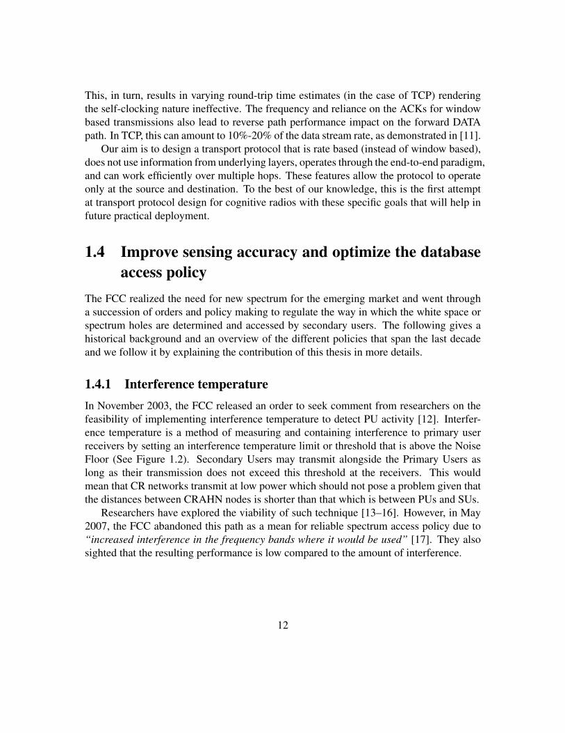
1.1 Cognitive cycle [1] . . . . . . . . . . . . . . . . . . . . . . . . . . . . . 91.2 Interference temperature threshold above the Noise Floor . . . . . . . . . 13

2.1 Throughput comparison between TCP and TFRC in a 3-hop chain ad-hocnetwork . . . . . . . . . . . . . . . . . . . . . . . . . . . . . . . . . . . 21

2.2 Method of sample collection in TFRC: the first dropped packet after anRTT concludes a sample. A received packet is denoted by an arrow and adropped packet by x . . . . . . . . . . . . . . . . . . . . . . . . . . . . . 24

2.3 Wired vs. wireless most recent sample (xi) size over a two-hop networktopology . . . . . . . . . . . . . . . . . . . . . . . . . . . . . . . . . . . 27

2.4 TFRC-CR finite state machine. Shaded states involve rate modificationsdiscussed in Section 2.5.2 . . . . . . . . . . . . . . . . . . . . . . . . . . 29

2.5 Throughput (kbps) vs Time for 3-hop (long PU activity) . . . . . . . . . . 332.6 Method of sample collection in TFRC-CR; instead of relying on the first

dropped packet, sample collection is based on a static time interval . . . . 342.7 Optimal multiplier M value for a 3 and 4-hop topologies . . . . . . . . . 362.8 3-Hop chain and PU region . . . . . . . . . . . . . . . . . . . . . . . . . 382.9 Sending rate Xbps during PU activity region . . . . . . . . . . . . . . . . 392.10 Throughput comparison as PU on time increases for different number of

hops . . . . . . . . . . . . . . . . . . . . . . . . . . . . . . . . . . . . . 402.11 Throughput comparison as PU on time increases for 2 and 3 hop scenarios

(TCP & TFRC) . . . . . . . . . . . . . . . . . . . . . . . . . . . . . . . 412.12 The interference, throughput and goodput comparison are provided in (a),

(b) and (c), respectively . . . . . . . . . . . . . . . . . . . . . . . . . . . 422.13 Throughput and queue length (for node 3) comparisons under different

stress events: none, congestion, bandwidth increase and bandwidth decrease 432.14 Throughput as the number of streams and PUs change, respectively . . . 44

5

3.1 Network architecture with two BSs A and B that have spectrum databaseaccess, and two vehicles C and D moving from left-right in a horizontalplane . . . . . . . . . . . . . . . . . . . . . . . . . . . . . . . . . . . . . 50

3.2 The traversed path in our measurement experiment with markers indicat-ing locations of high RSSI correlation between TV channels and 2G spec-trum (a), and explanation for the correlation (b) . . . . . . . . . . . . . . 52

3.3 Spectrum correlation between one TV channel band and one 2G radiotower RSSI values . . . . . . . . . . . . . . . . . . . . . . . . . . . . . . 54

3.4 Four different types of RSSI readings performed by sensing . . . . . . . . 553.5 Decision tree of the cognitive radio node. Solid lines indicate a possible

outcome while the dotted lines indicate the impossible ones . . . . . . . . 553.6 Sensing vs. Querying decision flow chart . . . . . . . . . . . . . . . . . 593.7 Interference alignment with three transmitters (A, B, C) and two intended

receivers (C, D) . . . . . . . . . . . . . . . . . . . . . . . . . . . . . . . 603.8 Number of spectrum-correlation points as the time of the experiment in-

creases . . . . . . . . . . . . . . . . . . . . . . . . . . . . . . . . . . . . 633.9 Number of queries for various spectrum correlation percentages . . . . . 643.10 Accuracy of sensing . . . . . . . . . . . . . . . . . . . . . . . . . . . . . 653.11 Channel utilization per vehicle for no IA allowed, IA allowed and pure

query scenarios in (a) light density and fast moving vehicles, (b) light den-sity and slow moving vehicles, (c) high density and fast moving vehiclesand (d) high density with slow moving vehicles . . . . . . . . . . . . . . 66

3.12 Channel utilization per vehicle (a) density and (b) velocity changes, re-spectively . . . . . . . . . . . . . . . . . . . . . . . . . . . . . . . . . . 68

3.13 Number of queries as the SNR increases . . . . . . . . . . . . . . . . . . 69

4.1 Cognitive cycle [1] . . . . . . . . . . . . . . . . . . . . . . . . . . . . . 744.2 The main building blocks of the proposed extension . . . . . . . . . . . . 754.3 New layered architecture of an ns-3 CR node . . . . . . . . . . . . . . . 784.4 State machine of the RX interface . . . . . . . . . . . . . . . . . . . . . 794.5 UDP flow’s throughput vs. time in a CR network. Gray areas indicate PU

activity . . . . . . . . . . . . . . . . . . . . . . . . . . . . . . . . . . . 804.6 Simulated CR network topologies (a) and (b) . . . . . . . . . . . . . . . 814.7 Memory utilization vs. total CPU execution time (kernel + userspace) for

both NS3 and CRE-NS3 . . . . . . . . . . . . . . . . . . . . . . . . . . 824.8 Total CPU execution time (kernel + userspace) for both CRE-NS3 and

CRAHN . . . . . . . . . . . . . . . . . . . . . . . . . . . . . . . . . . . 834.9 Memory utilization (MB) for both CRE-NS3 and CRAHN . . . . . . . . 83

6

List of Tables

1.1 Example results from different database administrators at the NortheasternUniversity campus . . . . . . . . . . . . . . . . . . . . . . . . . . . . . 16

2.1 Comparison between TFRC-CR and related works . . . . . . . . . . . . 24

3.1 Comparison between our architecture and related works . . . . . . . . . . 493.2 Interference alignment equations for node C . . . . . . . . . . . . . . . . 613.3 Interference alignment equations for node D . . . . . . . . . . . . . . . . 613.4 Interference alignment equations for node A . . . . . . . . . . . . . . . . 623.5 Interference alignment equations for node B . . . . . . . . . . . . . . . . 62

4.1 Comparison between CRE-NS3 and related works . . . . . . . . . . . . . 72

7

Chapter 1

Introduction

1.1 Cognitive radio, the motivation and definitionData spectrum is a finite natural resource. Ever since the introduction of wireless devices,the demand for faster data and larger bandwidth has been increasing at a rapid rate. Forexample, global mobile data traffic grew 70 percent in 2012 and mobile network speedsmore than doubled in 2012 [2]. The number of wireless subscribers world-wide is alsoexploding. The number of mobile subscribers grew 45 percent from 2012 to 2013 [3].New mobile devices and tablets with higher resolution displays are on the rise and so is thedemand for high definition content streaming, which require higher wireless data rates onthese congested airwaves. There is also a new generation of connected wireless servicesthat are being increasingly adopted, such as sensors, data streaming TVs, and satelliteconnected phones, among others, which contribute to the spectrum scarcity problem.

There are two possible ways to handle this new demand; one is to increase the numberof vacant spectrum that mobile users are allowed to use and the other is to improve theway in which we access what is currently available. In November 2002, the Federal Com-munications Commission (FCC), which is the government body that manages and licensesspectrum access in the United States, has published a report that aims at improving the wayin which this precious resource is used [4]. One of the major findings in that report is thatthe effective utilization of the current spectrum access poses problem comparable to theactual physical scarcity of the spectrum. In other words, the available physical spectrumcannot be neglected; efficient ways to utilize this existing spectrum, and new principles ofsharing spectrum are also needed.

Studies have revealed that while unlicensed spectrum utilization is high at most urbanplaces, some other bands remain largely or partially unoccupied [5–7]. These temporal orspatial unoccupied channels provide for an opportunity to relief the spectrum congestion

8

SpectrumSpectrum

Spectrum

Spectrum

Mobility

Sharing

Sensing

Decision

Environment

Radio

Channel

Capacity

TransmittedSignal

Primary UserDetection

Spectrum HoleDecisionRequest

SpectrumCharacterization

Figure 1.1: Cognitive cycle [1]

problem. An example of such channels are the digital broadcast television spectrum. Wewill refer to such channels of spectrum as “white space” where Secondary Users (SUs)may use the channel if it is left vacant by the TV broadcaster, or Primary Users (PUs).This new complex nature of when and how to access these white spaces necessitates a newtype of RF radio that is aware of its surroundings and can act based on observations it findsfrom the environment in which it is deployed in. All the above concerns motivate the useof the emerging technology called cognitive radio, which we describe next in detail.

1.1.1 Cognitive RadioThe term cognitive radio (CR) was first coined by Mitola III et. al. in 1999 [8] to de-scribe a radio node that is able to observe the environment surrounding it, learn from theparameters obtained, plan and orient itself for possible actions, decide the set of actionsto perform next and finally act on them. Later in 2005, Haykin [9] officially defined thecognitive radio as:“Cognitive radio is an intelligent wireless communication system that is aware of its sur-rounding environment (i.e., outside world), and uses the methodology of understanding-by-building to learn from the environment and adapt its internal states to statistical variationsin the incoming RF stimuli by making corresponding changes in certain operating param-eters (e.g., transmit-power, carrier-frequency, and modulation strategy) in real-time, with

9

two primary objectives in mind:

• highly reliable communications whenever and wherever needed;

• efficient utilization of the radio spectrum.”

A cognitive radio adhoc network (CRAHN) [1] is a network where the nodes commu-nicate with each other directly without a central infrastracture or base station. Each nodein CRAHN performs a cognition cycle (See Figure 4.1 [1, 8, 9]). The four main cognitivemanagement functions are:

• Spectrum sensing: The cognitive radio nodes sense the medium they are currentlytuned to to determine whether a primary user is occupying the channel. Based on theoutcomes of the sensing process, the spectrum holes (if available) are determined.When the nodes perform sensing, no transmission may be possible, and hence, sens-ing causes disruption to ongoing data connections.

• Spectrum decision: The radio must select one of the vacant spectrum holes to trans-mit in based on different metrics such as Quality Of Service (QoS). For example, anode may select a spectrum hole that is least occupied by other SUs.

• Spectrum sharing: given that multiple SUs might be concurrently occupying thesame spectrum hole, Medium Access Control (MAC) implementations are neces-sary. Through this function block, nodes may coordinate their sensing, transmissionand idle times to reduce interference with the PU and the vacant time of the channeltime.

• Spectrum mobility: Once a node determines the next channel to transmit on, it needsto be able to handoff the current channel and switch to it. This incurs an additionalspectrum switching delay.

The contributions of this thesis towards enhancing spectrum efficiency in the currentunlicensed band, and identifying the licensed frequencies for opportunistic use are statedbelow.

1.2 Main contributions of this thesis• Chapter 2 - Cognitive radio transport layer design: We design an equation-based

transport protocol that relies on the FCC database to improve the data transmissionrate, reduce congestion and enable fast response time in the specialized scenarios ofmulti hop CRs.

10

• Chapter 3 - Improve sensing accuracy and optimize the database access policy:We devise a novel method to improve the accuracy of sensing by leveraging crosscorrelation information between 2G cellular and TV whitespace spectrum. We alsopropose an efficient spectrum access policy that uses Interference Alignment andFull-Duplex technologies to shorten the time it takes to transmit CR control mes-sages. Both these techniques are demonstrated for a practical case of vehicular CRnetworks.

• Chapter 4 - A cognitive radio module for the network simulator 3: We develop acomprehensive simulation framework for ns-3, which provides ready access to sev-eral advanced CR features, such spectrum sensing, spectrum decision and mobility,allows multiple link layers and interfaces and also enables studies on coexisting CRand non-CR nodes. This new module is compared against existing work in ns-2 andthe code modules are released for further development by the research community.

1.3 Cognitive radio transport layer designWhile the main functional blocks of spectrum sensing, switching, and sharing have expe-rienced rapid strides over the past decade [1], work on higher layers of the protocol stack,such as the transport layer that is essential for realizing large scale practical deployments,remains in a nascent stage.

To date, the work on CR transport protocols has been based on the TCP window-behavior, where the acknowledgement packets (ACKs) sent by the received determine thestate of congestion within the network [10]. This self-clocking mechanism of TCP ishighly susceptible to the observed round trip time. With periodic interruptions caused byprimary user appearance, or large scale bandwidth fluctuations, this mechanism by itselfis unable to distinguish true congestion from PU induced spectrum changes. These worksthat directly adapt TCP for CR networks, rely on comprehensive information from theunderlying layers, as well as the intermediate nodes of the route. While there are distinctmerits in a cross-layer approach, such a design violates the traditional end-to-end paradigmassociated with the transport layer.

Chapter 2 of this thesis presents a fresh perspective on the design of CR-specific pro-tocol using an equation-based approach, wherein the concept of the congestion window inclassical TCP is eliminated, and instead, an equation is devised as a function of the effec-tive packet loss rate. This equation is not dependent on the time variance of the returningACKs, and hence, the source transmission rate is less impacted by temporary disruptions inthe flow. This problem of reliance on ACK timing is exacerbated in CR networks becausenodes pause their transmission when they are engaged in sensing or channel switching.

11

This, in turn, results in varying round-trip time estimates (in the case of TCP) renderingthe self-clocking nature ineffective. The frequency and reliance on the ACKs for windowbased transmissions also lead to reverse path performance impact on the forward DATApath. In TCP, this can amount to 10%-20% of the data stream rate, as demonstrated in [11].

Our aim is to design a transport protocol that is rate based (instead of window based),does not use information from underlying layers, operates through the end-to-end paradigm,and can work efficiently over multiple hops. These features allow the protocol to operateonly at the source and destination. To the best of our knowledge, this is the first attemptat transport protocol design for cognitive radios with these specific goals that will help infuture practical deployment.

1.4 Improve sensing accuracy and optimize the databaseaccess policy

The FCC realized the need for new spectrum for the emerging market and went througha succession of orders and policy making to regulate the way in which the white space orspectrum holes are determined and accessed by secondary users. The following gives ahistorical background and an overview of the different policies that span the last decadeand we follow it by explaining the contribution of this thesis in more details.

1.4.1 Interference temperatureIn November 2003, the FCC released an order to seek comment from researchers on thefeasibility of implementing interference temperature to detect PU activity [12]. Interfer-ence temperature is a method of measuring and containing interference to primary userreceivers by setting an interference temperature limit or threshold that is above the NoiseFloor (See Figure 1.2). Secondary Users may transmit alongside the Primary Users aslong as their transmission does not exceed this threshold at the receivers. This wouldmean that CR networks transmit at low power which should not pose a problem given thatthe distances between CRAHN nodes is shorter than that which is between PUs and SUs.

Researchers have explored the viability of such technique [13–16]. However, in May2007, the FCC abandoned this path as a mean for reliable spectrum access policy due to“increased interference in the frequency bands where it would be used” [17]. They alsosighted that the resulting performance is low compared to the amount of interference.

12

Figure 1.2: Interference temperature threshold above the Noise Floor

1.4.2 Local and cooperative spectrum sensingIn December 2003, the FCC released an order requesting a comment on the feasibilityof implementing a cognitive radio network that may use cooperative and local sensing todetect PU activity and use the sensed primary channel when it is detected to be idle [18].

Since this release, researchers have proposed frameworks and algorithms that exploittemporal [19,20] and spatial [21–23] white space access opportunities using collaboration.Most of the work in these papers focused on the optimization of dividing spectrum acrossnodes but assumed either perfect knowledge of the spectrum opportunities available to theSUs or perfect sensing. For example, [22] proposed a collaborative scheme to optimizespectrum allocation using a color-sensitive graph coloring model to characterize the spec-trum access problem and provides rules for SUs to use to avoid interference with the PU.In [24], the authors make a comparison between centralized strategy where a server allo-cates spectrum for CRs and a distributed system where CRs collaborate to negotiate thelocal spectrum assignment. In [25], a framework is deviced that pits nodes that organizethemselves into clusters. These clusters of nodes then choose spectrum based on the globaloptimal assignment.

Some work was also done on optimizing local sensing. For example, in [26], Chen etal. integrated the MAC spectrum access policy with physical layer sensing to optimize thethroughput for SUs under the constraint of a collision threshold as perceived by the PU.

In 2010 [27], the FCC withdrew the sensing requirement: “However, at this juncture,we do not believe that a mandatory spectrum sensing requirement best serves the publicinterest. As petitioners and responding parties indicate, the geo-location and databaseaccess method and other provisions of the rules will provide adequate and reliable protec-

13

tion for television and low power broadcast auxiliary services, so that spectrum sensing isnot necessary”. However, this order did not completely eliminate the need for spectrumsensing: “We anticipate that some form of spectrum sensing may very well be includedin TVBDs (TV Band Devices) on a voluntary basis for purposes such as determining thequality of each channel relative to real and potential interference sources and enhancingspectrum sharing among TVBDs” [27].

This database mandate will be used throughout Chapters 2 and 3 of this thesis. Thenext section will give an overview of the database structure and of currently deployeddatabases.

1.4.3 The FCC databaseIn November 2011, the FCC has released a landmark ruling [27] that mandated the useof spectrum database access. These rulings contained specifics for mobile and stationarycognitive radio devices to follow before accessing any free white band TV spectrum intheir vicinity.

The FCC ruling categorized the types of devices that may access the database into thefollowing:

• Fixed devices

• Mode I

• Mode II

• Sensing only devices

Fixed devices

Fixed devices operate from a stationary location. Uses for such devices range from WiFiHotspots, rural broadband distribution to cellular-style installations. These devices typ-ically operate with high power and are installed in high terrain locations or on top ofbuildings. As such, the database returns different results for these types of devices giventhat the signals from such devices propagate over longer distances and can affect multiplechannels due to the relatively high signal strength.

Portable devices

Mode I, II and Sensing only devices can be all categorized as portable devices. The dis-cussion on the difference between these types of devices will follow later. These types of

14

devices operate at lower transmission power relative to fixed devices. Due to the shorterpropagation paths for these devices, the spectrum database returns more channels or bandsfor these devices to utilize. The transmission power limit on these devices is 40 mW or16dBm. Some examples of such devices: laptops, Wifi Access Points (AP), tablets andsmartphones.

The databases

As of this writing, there are currently ten FCC database managers or administrators. InJanuary 26, 2011, the FCC approved the following companies to manage the spectrumdatabases: Comsearch, Frequency Finder Inc., Google Inc., KB Enterprises LLC and LSTelcom, Key Bridge Global LLC, Neustar Inc., Spectrum Bridge Inc., Telcordia Tech-nologies, and WSdb LLC [28]. However, in April 18, 2011, Microsoft applied to join thegroup [29] and got approved to do so in July 29, 2011 [30].

The database structure

To date, only four of the ten approved database managers have websites that allow forfree public testing [31]. These companies are Key Bridge Global, Google Inc., SpectrumBridge and Telcordia. The database for these sites is similar: they categorize the list ofdevices into Fixed, Portable and Microphones. One can put the coordinates of a specificlocation, select the type of device and search for the results. The results highlight the listof available channels that this specific type of device may use.

For fixed devices, the Height Above Average Terrain (HAAT) is returned along withthe allowed height for this fixed device installation. In all sites, the allowed antenna heightabove ground level has to be less than 30 meters.

Microphones and portable devices operate in the same frequencies due to the lowpower allowed to transmit, which is 16 dBm. The only difference between the two isthat Microphone devices are allowed to reserve a channel for exclusive use for a certainperiod. The databases also let portable and microphone devices that query it know whichof these free channels are currently reserved by a microphone, and therefore, may not beused.

We conducted a study in March 2011 between all available public databases. Thelocation in question was Forsyth St, in the Northeastern University campus. The resultsare shown in Table 1.1.

15

Database Fixed devices Height (AGL) Power Portable Devices PowerKey bridgeglobal [32]

2, 5, 6, 7 3 m (default) N/A 23, 24, 26, 28, 33,34, 44, 46, 48, 50

low

Google, Inc. [33] 2, 5, 6, 7 10 m (default) 36 dBm 23, 24, 26, 28, 44,46, 48, 50

16 dBm

SpectrumBridge [34].

2, 5, 6, 7 30 m N/A 23, 24, 26, 28, 44,46, 48, 50

16 dBm

FrequencyFinder, Inc. [35]

No public database

KB Enterprises,Inc. [36]

No public database

NeuStar, Inc. [37] No public databaseTelecordiaTech [38].

2, 5, 6, 7 N/A N/A 23, 24, 26, 28, 44,46, 48, 50

16 dBm

WSdb, Inc. [39] No public databaseMicrosoft,Inc. [40]

No public database for USA

Comsearch. [41] No public database

Table 1.1: Example results from different database administrators at the Northeastern Uni-versity campus

16

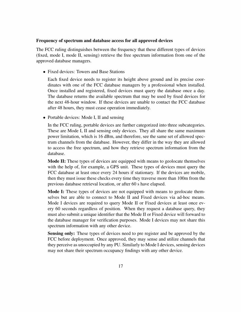
Frequency of spectrum and database access for all approved devices

The FCC ruling distinguishes between the frequency that these different types of devices(fixed, mode I, mode II, sensing) retrieve the free spectrum information from one of theapproved database managers.

• Fixed devices: Towers and Base Stations

Each fixed device needs to register its height above ground and its precise coor-dinates with one of the FCC database managers by a professional when installed.Once installed and registered, fixed devices must query the database once a day.The database returns the available spectrum that may be used by fixed devices forthe next 48-hour window. If these devices are unable to contact the FCC databaseafter 48 hours, they must cease operation immediately.

• Portable devices: Mode I, II and sensing

In the FCC ruling, portable devices are further categorized into three subcategories.These are Mode I, II and sensing only devices. They all share the same maximumpower limitation, which is 16 dBm, and therefore, see the same set of allowed spec-trum channels from the database. However, they differ in the way they are allowedto access the free spectrum, and how they retrieve spectrum information from thedatabase.

Mode II: These types of devices are equipped with means to geolocate themselveswith the help of, for example, a GPS unit. These types of devices must query theFCC database at least once every 24 hours if stationary. If the devices are mobile,then they must issue these checks every time they traverse more than 100m from theprevious database retrieval location, or after 60 s have elapsed.

Mode I: These types of devices are not equipped with means to geolocate them-selves but are able to connect to Mode II and Fixed devices via ad-hoc means.Mode I devices are required to query Mode II or Fixed devices at least once ev-ery 60 seconds regardless of position. When they request a database query, theymust also submit a unique identifier that the Mode II or Fixed device will forward tothe database manager for verification purposes. Mode I devices may not share thisspectrum information with any other device.

Sensing only: These types of devices need to pre register and be approved by theFCC before deployment. Once approved, they may sense and utilize channels thatthey perceive as unoccupied by any PU. Similarly to Mode I devices, sensing devicesmay not share their spectrum occupancy findings with any other device.

17

In Chapter 3 of this thesis, we show how the sensing accuracy can be optimized byleveraging cross-correlation information from different spectrum channels. We then lever-age this increase of accuracy to improve on the database spectrum access policy by relyingon a combination of database accesses and spectrum sensing to reduce the cost and amountof required database querying in a vehicular cognitive ad-hoc network.

In the second half of Chapter 3, we also make use of interference alignment [42].Interference alignment is an emerging technology that is able to separate useful signalsfrom interfering ones into orthogonal planes. This allows a combination of messages tobe sent simultaneously into one time slot, leading to better utilization of the channel andpower efficiency. We provide to the best of our knowledge, the first real-world applicationof interference alignment to allow for shortened channel utilization and better efficiencyin the control channel in the cognitive vehicular network that we propose.

1.5 A cognitive radio module for the network simulator 3Networking engineers and researchers contributing in the emerging area of cognitive ra-dio researchers face uphill challenges when testing a new concept, given the challengingenvironment in which these networks operate. The CRs must opportunistically determinewhich licensed channels are available and make use of this spectrum before the licenseduser reclaims it. Accurate protocol operation is critical, as any prolonged use of the chan-nel raises concerns of interfering with the activities of the licensed users. This concerndirectly translates to meticulous testing of the protocol or networking concept in a con-trolled environment. Given the uphill costs of purchasing multiple software defined radiosthat serve as the hardware building blocks of the CR network, and the time investment iswriting and deploying code in them, computer simulation often becomes the methodologyof choice.

While several commercial simulators exist, such as OPNET [43], which can capablysimulate heterogenous networks, our focus in this work remains on affecting improve-ments to open-source simulators. The main challenges in such environment are as follows:

• CR protocols are generally cross-layered. Any change in one layer, such as spectrumsensing duration at the physical layer (PHY), has direct impact on the decisionsmade in the upper layers of the protocol stack, requiring extensive code changesthroughout the stack.

• The testing time increases dramatically with the complexity of the protocol. Owingto the large number of variables that can be controlled, identifying the dominatingfactor that impacts the environment to the greatest possible extent may force largenumber of trial runs.

18

• The inter-dependence of the protocol layers requires network architects to imple-ment more than one layer. For e.g., spectrum sensing at the PHY can impact theTCP throughout and its interpretation of congestion. Thus, the expertise required tosimulate CR networks effectively is more than conventional wireless networks.

• New functions unique to the area of CR, such as spectrum sensing, spectrum hand-off and licensed or primary user (PU) detection need to be embedded in the simula-tor.

The focus of Chapter 4 is on providing the first cognitive radio extension to the net-work simulator 3 [44] or ns-3, which is a discrete event driven simulator. This simulatoris poised to replace the widely popular predecessor, network simulator 2 or ns-2. Ns-3 offers several advantages over ns-2, including: (i) it has a new core written in C++,(ii) it is geared for wireless communications, (iii) it has an organized modular architec-ture that is expandable, (iv) it includes intuitive and extensive documentation via the htmlDoxygen [45] interface, and (v) the same ns-3 code can be easily adapted to work in realdevices [44].

19

Chapter 2

Cognitive radio transport layer design

2.1 Problem overviewCognitive radio networks enable opportunistic use of available licensed spectrum to reducethe pressure on the unlicensed ISM bands in the 2.4GHz and 5GHz range. While themain functional blocks of spectrum sensing, switching, and sharing have experienced rapidstrides over the past decade [1], work on higher layers of the protocol stack, such as thetransport layer that is essential for realizing large scale practical deployments, remains ina nascent stage.

To date, the work on CR transport protocols has been based on the TCP window behav-ior, where the acknowledgment packets (ACKs) sent by the receiver determine the stateof congestion within the network [10, 46, 47]. This self-clocking mechanism of TCP ishighly susceptible to the observed round trip time. With periodic interruptions caused bythe primary user’s appearance or large scale bandwidth fluctuations, this mechanism byitself is unable to distinguish true congestion from PU induced spectrum changes. Theseworks that directly adapt TCP for CR networks rely on comprehensive information fromthe underlying layers, as well as the intermediate nodes of the data path route. Whilethere are distinct merits in a cross-layer approach, such a design violates the traditionalend-to-end paradigm associated with the transport layer.

In window-based transport protocols, the problem of reliance on ACK timing is exac-erbated in CR networks because nodes pause their transmission when they are engaged insensing or channel switching. This, in turn, results in varying round-trip time estimates(in the case of TCP) rendering the self-clocking nature ineffective. The frequency andreliance on the ACKs for window based transmissions also lead to reverse path perfor-mance impact on the forward DATA path. In TCP, this can amount to 10%-20% of thedata stream rate as demonstrated in [11]. This work presents a fresh perspective on the

20

0

20

40

60

80

100

120

140

160

180

10 20 30 40 50 60 70 80 90 100

Thro

ughput (k

bps)

time (seconds)

TFRC vs TCP throughput

TCP ThroughputTFRC Throughput

Figure 2.1: Throughput comparison between TCP and TFRC in a 3-hop chain ad-hocnetwork

design of CR-specific protocols using an equation-based approach, wherein the concept ofthe congestion window in classical TCP is eliminated, and instead, an equation is devisedas a function of the effective packet loss rate. This equation is not dependent on the timevariance of the returning ACKs, and hence, the source transmission rate is less impactedby temporary disruptions in the flow.

The authors of [11] also report that CSMA/CA at the link layer results in bursty end-to-end flows when coupled with TCP at the transport layer. We independently verify thisin Figure 2.1 for a three node network where no congestion is introduced. The observedincrease in TCP throughput may not only cause a potential adverse impact to the CR net-work through congestion, but also to the PUs by interfering with their packet deliveryperformance. Instead, the equation based TCP Friendly Rate Control (TFRC), a represen-tative of the broader class of equation based transport protocol [48], remains stable, and inthe absence of any other external stimulus, avoids the bursty transmissions seen in TCP.

Our approach towards transport protocol design for CR follows a new direction ofusing an equation based control, hitherto unexplored in the current literature. For this, weuse the TFRC as the departure point. We not only adapt the state-action behavior of TFRC,but also modify the actual rate control equation leading to our new design for CR that wename as TFRC-CR. The main features of this new protocol are as follows:

• It allows the TCP source to integrate with designated spectrum databases, as man-dated by the FCC in a recent ruling [27]. This limited (and required) interaction withthe database totally removes any need of feedback from the intermediate nodes or

21

from the underlying layers. Thus, TFRC-CR reverts back to the classical end-to-endparadigm associated with the transport layer.

• It intelligently polls the spectrum database only when needed, by identifying a pos-sible PU arrival event based on the observed trend in packet losses, i.e., it does notconsume the back-end system resources used for interacting with the database. Cur-rent regulations from FCC specify database polling at least once every 60 secondsfor Mode I devices (more on that in Section 2.5), and our aim is to increase theaccess frequency only when a critical need is detected.

• It enhances the speed of response by distinguishing between spectrum change andtrue congestion. Hence, the transmission rate is almost never penalized unless theneed is justified. Likewise, the rate of increase in the transmitted segments whennew spectrum becomes available is much higher than that possible in the classicalwindow based TCP, owing to the immediate effect of the rate equation.

• It modifies the TFRC rate control equation by changing the definition of the loss-event interval. This change allows the protocol to utilize the bandwidth more effi-ciently by having a higher and more accurate sending rate and throughput.

The rest of this chapter is organized as follows: Section 4.2 gives the related works inthe area of transport protocol design for CR. The preliminary background of TFRC andthe motivation for adapting it for CRs is described in Sections 2.3 and 2.4. In Section 2.5,we describe the proposed protocol (TFRC-CR) in detail. Section 2.6 gives results fromour comprehensive simulation study, and finally, we conclude our chapter in Section 3.7with pointers to future research.

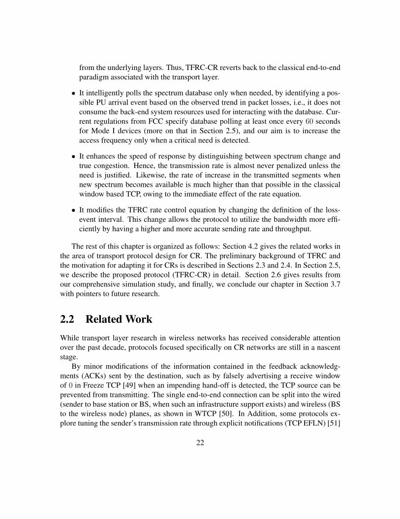
2.2 Related WorkWhile transport layer research in wireless networks has received considerable attentionover the past decade, protocols focused specifically on CR networks are still in a nascentstage.

By minor modifications of the information contained in the feedback acknowledg-ments (ACKs) sent by the destination, such as by falsely advertising a receive windowof 0 in Freeze TCP [49] when an impending hand-off is detected, the TCP source can beprevented from transmitting. The single end-to-end connection can be split into the wired(sender to base station or BS, when such an infrastructure support exists) and wireless (BSto the wireless node) planes, as shown in WTCP [50]. In Addition, some protocols ex-plore tuning the sender’s transmission rate through explicit notifications (TCP EFLN) [51]

22

and via selective retransmissions of lost packets (TCP SACK) [52]. While each of theseapproaches have merits, they were not originally designed with the aim of licensed orprimary user protection, sudden large-scale bandwidth fluctuations, and periodic interrup-tions caused by spectrum sensing and channel switching.

More specific to cognitive radio, various measurement studies have demonstrated theneed for a new transport protocol for cognitive radio networks (CRNs) [46, 53, 54]. Inparticular, the suitability of TCP for CR networks, given its widespread use, has been ex-plored in [46, 53–56]. The work in [46] proposes modifications to TCP and introducesthree different protocols: cogTCP, cogTCPE and cogTCPW. The knowledge module com-mon to all of the above is linked to the transport protocol that leverages information fromthe link and physical layer such as sensing times and estimated bandwidth. This family ofprotocols is designed for single hop scenarios.

Other protocols that leverage cross-layer information [57–60] also exist in literature.DSAsync [59] is a framework that modifies the base station’s link layer that connectsthe outer wired network to the inner cognitive radio environment. It uses informationfrom the link layer to explicitly pause the source and destinations’ TCP streams, and isfocused on a centralized (1-hop) topology between the CR nodes and the BS. Similarlyto DSASync, [60] proposes modifications to the Base Station that connects TCP over theinternet to a Cognitive Radio network by modifying the Base Station by two proposedmethods: a) Local loss recovery by base station and b) Split TCP connection. The CRnetwork is a one-hop network and the proposal restricts its modifications to the base stationand not the transport protocol layer in the cognitive radio nodes. TP-CRAHN uses awindow based approach similar to TCP, relies on intermediate node feedback and uses across-layer approach in each node involved [10]. TCP-CReno [47] modifies TCP Reno sothat it pauses and resumes the data when the node is performing sensing. This informationis retrieved from the MAC layer.

Protocols that change lower network layers to improve throughput at the transport lay-ers were also investigated [57, 58, 61]. In [57], Luo et al. optimize the throughput ofTCP by using an algorithm to decide which channel to use. Optimization at the physi-cal, MAC, and link layer such as sensing times, access decision, modulation and codingscheme, and link layer frame size were also done in [58]. In [61], changes to the sens-ing and transmission times of the CR nodes were done to improve the throughput at TCP.These frameworks do not propose a new transport protocol, but improve the throughputby changing lower network layer parameters.

Different from all of the above, our aim is to design a transport protocol that is ratebased, does not use information from underlying layers, operates through the end-to-endparadigm, and can work efficiently over multiple hops. These features allow the protocolto operate only at the source and destination. To the best of our knowledge, this is the

23

Protocol CR Eq. Based Multihop No cross layer End-to-End No mod. tolow layers

Freeze TCP [49] ✓ ✓ ✓ ✓

WTCP [50] ✓ ✓ ✓

TCP EFLN [51] ✓ ✓ ✓ ✓

TCP SACK [52] ✓ ✓ ✓ ✓

[57–61] ✓ ✓ ✓

TCP-Creno [47] ✓ ✓ ✓

CogTCP/E/W [46] ✓ ✓ ✓

TP-CRAHN [10] ✓ ✓ ✓

TFRC-CR ✓ ✓ ✓ ✓ ✓ ✓

Table 2.1: Comparison between TFRC-CR and related works

xi i−1

x

RTT RTT

Figure 2.2: Method of sample collection in TFRC: the first dropped packet after an RTTconcludes a sample. A received packet is denoted by an arrow and a dropped packet by x

first attempt at transport protocol design for cognitive radios with these specific goals. Weare hopeful that will help in future practical deployment. Table 2.1 shows a summary andcomparison between our proposed protocol and the related ones discussed above.

2.3 Discussion on Rate Control in TFRCTFRC employs equation based congestion control in unicast traffic. We use this as theplatform to build our protocol because it aims at providing a stable throughput, as opposedto the sudden fluctuations caused by the additive increase multiplicative decrease behaviorof TCP. Given that TFRC is rate based, we also have finer grain control over the sendingrate. We begin by describing the classical rate control equation in TFRC.

Let xi be the number of consecutive packets delivered to the destination in the ith

sample. The counting of these packets for the calculation of xi continues till the first loss

24

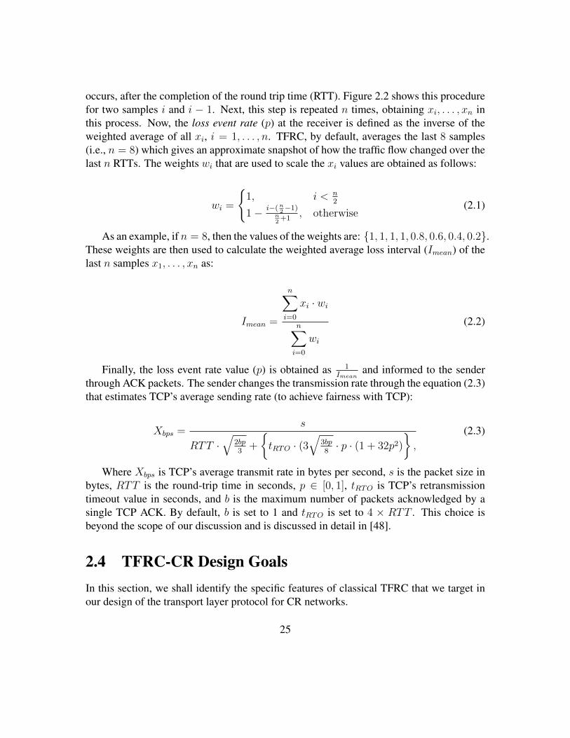
occurs, after the completion of the round trip time (RTT). Figure 2.2 shows this procedurefor two samples i and i − 1. Next, this step is repeated n times, obtaining xi, . . . , xn inthis process. Now, the loss event rate (p) at the receiver is defined as the inverse of theweighted average of all xi, i = 1, . . . , n. TFRC, by default, averages the last 8 samples(i.e., n = 8) which gives an approximate snapshot of how the traffic flow changed over thelast n RTTs. The weights wi that are used to scale the xi values are obtained as follows:

wi =

�1, i < n

2

1− i−(n2−1)

n2+1

, otherwise(2.1)

As an example, if n = 8, then the values of the weights are: {1, 1, 1, 1, 0.8, 0.6, 0.4, 0.2}.These weights are then used to calculate the weighted average loss interval (Imean) of thelast n samples x1, . . . , xn as:

Imean =

n�

i=0

xi · wi

n�

i=0

wi

(2.2)

Finally, the loss event rate value (p) is obtained as 1Imean

and informed to the senderthrough ACK packets. The sender changes the transmission rate through the equation (2.3)that estimates TCP’s average sending rate (to achieve fairness with TCP):

Xbps =s

RTT ·�

2bp3

+

�tRTO · (3

�3bp8

· p · (1 + 32p2)

�,

(2.3)

Where Xbps is TCP’s average transmit rate in bytes per second, s is the packet size inbytes, RTT is the round-trip time in seconds, p ∈ [0, 1], tRTO is TCP’s retransmissiontimeout value in seconds, and b is the maximum number of packets acknowledged by asingle TCP ACK. By default, b is set to 1 and tRTO is set to 4 × RTT . This choice isbeyond the scope of our discussion and is discussed in detail in [48].

2.4 TFRC-CR Design GoalsIn this section, we shall identify the specific features of classical TFRC that we target inour design of the transport layer protocol for CR networks.

25

2.4.1 Low utilization of available bandwidthTFRC reduces the sending rate at the source whenever packets are dropped in the sendingsequence. This simplistic approach is sufficient for wired networks, where packets areonly dropped due to congestion, but not in CR networks where drops can happen due tomultiple factors. We explain the mechanism as follows, and identify possible ways toadapt this situation.

Equation 2.3 can be reduced to:

Xbps =s

RTT ·f(s)where

f(s) =�

2p3+ 12 ·

�3p8· p · (1 + 32 + p2)

(2.4)

When tRTO = 4 × RTT and b = 1, these are approximated to equal TCP’s sendingrate [48].

From equation 2.4, the two contributing factors to the sending rate are RTT and p, theloss event rate. As explained earlier p is the inverse of the weighted average of the sam-ples xi (see Equation 2.2). In wireless networks, the sample xi values tend to be smallerthan in wired networks. This is because TFRC assumes that dropped packets occur due tocongestion only (when intermittent losses are possible owing to channel errors). As soonas a single dropped packet is encountered at the receiver after an RTT has elapsed, thesample round i is completed, the value of xi is logged and computation for xi+1 beginsimmediately. Figure 2.2 describes this situation. The overall effect of this behavior is thatfor wired networks, this leads to relatively equal sample lengths, i.e., x1 ≈ · · · ≈ xn val-ues. However, and particularly in CR networks, the disparity in the samples xi is wider,as PU activity, spectrum availability changes, among other factors contribute to occasionalpacket losses. Figure 2.3 shows this divergent behavior for wired and wireless cases. Be-cause of this discrepancy in sample lengths in cognitive radio networks, TFRC’s sendingrate is fluctuating even when no stress events are introduced in the network. Our aim is toequalize the sample lengths by introducing a time-based sample collection method. Thiswill produce equal lengths when the network is in normal condition and will also adapt insize as the network’s available bandwidth changes.

2.4.2 Low transmission rate after PU departureClassical TFRC is unable to use the maximum allocated bandwidth after a PU vacates thespectrum due to the transmission source’s low rate that is caused by timeout events when aCR node ceases transmission or due to interference caused by PU activity. Instead, TFRC-CR is designed to neglect the last n loss event rates after a prolonged idle state due to PU

26

0

50

100

150

200

250

300

350

400

450

10 12 14 16 18 20 22 24 0

10

20

30

40

50

60

mo

st

rece

nt

sa

mp

le s

ize

(w

ire

d)

mo

st

rece

nt

sa

mp

le s

ize

(w

ire

less)

time (seconds)

TFRC (Wired vs Wireless sample values)

WiredWireless

Figure 2.3: Wired vs. wireless most recent sample (xi) size over a two-hop networktopology

activity. This prevents the pitfall of resuming the transmission with a false p which leadsto less than optimal throughput. Note that classical TFRC will recover to the maximumtransmission rate after at least n samples have been recorded. This takes at least n RTTsto achieve.

2.4.3 Slow recovery and ramp upAfter an extended period of packet losses that limit TFRC’s sending rate to the minimumrate, the protocol starts polling for changes in bandwidth over large intervals of time.This polling interval is a function of the current transmission rate. For example, duringPU Activity, classical TFRC’s nofeedback timer expires multiple times which leads toreduction in the effective rate by half each time until the minimum rate of s

tmbiis reached.

Here, s is the packet size and tmbi is set to 64 seconds in the default implementation.This means that TFRC will poll the network once every 64 seconds, which can cause anequivalent delay for the CR network to resume transmission again after a PU departure.Thus vital spectrum opportunity is wasted in this extended downtime for the CR network.Our goal is to speed the resurgence of the data flow by integrating the transport protocolwith the FCC database which can inform the sending node in advance the time at whichthe current PU activity ends.

27

2.4.4 Buffer overload and interferenceTFRC may send multiple packets during the duration of the PU activity as part of its reg-ular rate control which causes additional interference with the PU. This serious problemmultiplies at the link layer, where typically the medium access control protocol attemptsseveral rounds of transmission per packet before reaching the maximum retry limit. More-over, the added processing tasks as well as the consumption of buffer space by these addi-tional packets that cannot be transmitted on the same channel contribute to the overhead.While the CR network can be designed to seek out and immediately leverage alternatechannels, this feature is not known at the source in advance (owing to lack of inter-layercommunication). By relying on the FCC database to inform the sender of possible disrup-tions due to PU activity, this problem can be alleviated; the sender will pause the data flowbased on that information which will lessen the stress on the intermediate nodes’ queues.

2.5 Design and Implementation of TFRC-CRWe first present the modified finite state machine for TFRC-CR which we will refer toas we describe the overall functions related to spectrum management and PU avoidance.Then, we discuss how to change the rate equation in TFRC-CR such that the connectionsutilize the maximum allocated bandwidth.

Note about FCC database and connectivity: In [27], the FCC has recently alloweddifferent devices to use a centralized database to infer PU activity. Devices that are allowedto use the channels are categorized in three modes: Mode I, Mode II and sensing mode.Mode II are geolocation capable devices that are required to access the database directly atleast once per day before utilizing any channel, Mode I devices needs to connect to ModeII devices directly or a fixed-based station, and are required to refresh their local databaseinformation once every minutes. Sensing mode nodes need to be certified by the FCC andcan then sense and use what they perceive as vacant spectrum. In the design of TFRC-CR, we are only interested in spectrum awareness at end locations and do not involve theintermediate nodes. This still maintains the end-to-end sense of the transport protocol. Inany case, we do not rely on the knowledge of specifically ”where” or ”at which node”PU activity occurred in the connection, but that it occurred somewhere in the connection.Similar assumptions on rough estimations of a region of interest have been made in earlierworks on routing (see reference [62] for example).

28

PU

Resume

Paused

Detected

Normal

Start

Slow

PUExit

ACK

Tim

eout

Rec

eive

d a pa

cket

In average ACK inter−arrival

No ACK Received

ACK Received

No ACK

PU E

xits

& N

o ACK

Slow start A

CK received

Conditions met

Conditionsnot met

PU Exits

Figure 2.4: TFRC-CR finite state machine. Shaded states involve rate modifications dis-cussed in Section 2.5.2

2.5.1 TFRC-CR Spectrum ManagementThis section covers the following key features of our proposed protocol: (i) ensuring thatconnection immediately becomes active after the PU leaves the impacted region, (ii) strik-ing a balance between polling the network too frequently by the source, an action thatmay itself cause interference with the PU, and conversely, reacting too slowly to spec-trum change, and (iii) estimating the available bandwidth as soon as possible after thePU vacates the spectrum. These changes are explained below using a finite state machinediagram, shown in Figure 2.4.

Normal state

This is the default state of TFRC-CR. The protocol returns to this state whenever the sourceinfers the connection to be free of spectrum outages. We describe in detail how the equa-tion governing the sending rate (and hence, congestion control) in this state is modified

29

in Section 2.5.2. Recall that when a packet is dropped, the no feedback timer expires inthe absence of the ACK. From here onward, our protocol’s operation diverges from clas-sical TFRC: To differentiate congestion from possible PU activity at this timer expiry, thesource queries the FCC mandated spectrum database to check if a PU arrived on any ofthe feasible channels. Note that the source has no knowledge of the location of the nodesin the connection except the destination, nor the specific channels used by any of thesenodes. However, a sudden arrival event of the PU (as indicated by the database) and theresulting timeout are treated as correlated events. If the database affirms the PU presence,the protocol enters into the PU detected state, and if not, the ACK loss is interpreted as acase of network congestion and is handled by the standard TFRC rate control which cutsthe sending rate in half. In the normal state, the protocol continues to calculate the averageACK inter-arrival time (denoted as In), and the standard deviation of the round-trip time(denoted as RTTstddev). These values are used in the subsequent states to influence therate control mechanism.

Please note that our reliance on the ACK timer expiry to query the FCC databaseand infer PU activity here is different than congestion inference that is typically usedin window-based transport protocols; TFRC-CR’s end-destination periodically generatesACKs for the sender, whether or not (i) there is true network congestion, and (ii) packetarrival to the destination. Thus, the rate control is decoupled from the frequency of return-ing ACKs, which is the typical method used in window-based protocols. In TFRC-CR, ifa sender does not receive an ACK, then it signals a larger event, such as a total disruptionon the link. In this state, we use this scenario to map a PU appearing which renders thelink unusable.

PU detected state

This intermediate state is implemented as an additional measure to verify that the lastACK timeout in the normal state was in fact due to PU activity. Upon entering this state,the source waits for a period (the average inter-arrival time during normal state or In) forany incoming ACK, while continuously polling the spectrum database. If no subsequentACKs are received, and the database reveals that the PU is still present, then the protocoltransitions into the paused state where the source must wait for the PU activity to getcompleted. On the other hand, if an ACK does arrive in that time period, then the protocolreturns to the normal state as this implies that the intermediate nodes are not affected bythe PU activity. In such a case, the ACK timer expiry was due to random channel errors orcongestion.

30

Paused state

In this state, TFRC-CR determined that the PU is present and assumed that it is responsiblefor disrupting the continuous data stream. The challenge now is to identify when thetransmission rate can revert back to a higher value and this is obtained by polling theconnection with an occasional packet. When a portion of the spectrum is occupied by aPU, the link layer algorithms on the node pair on the affected link may either pause thetransmissions altogether, or immediately try and identify an alternate spectrum for thatlink. Note that the source has no idea which of these options is selected as no intermediatenode feedback is allowed. Additionally, simple monitoring of the spectrum database, evenif it indicates the presence of a PU, does not reveal any corrective action by the nodesin the connection. Thus, determining when the connection is active again is a non-trivialtask.

By increasing the transmission rate too early, the source risks added interference to thePU before it vacates the spectrum. Also, by delaying the rate increase, the source is unableto efficiently use the available bandwidth of the connection if the PU vacates the spectrumearlier or the nodes in the connection transition to a new channel. We have undertaken asubstantial set of simulations and empirically identify the optimal polling rate as

Xbps =s

RTTavg + 4×RTTstd

(2.5)

(Section 2.3), i.e., the source will send a packet every time the Retransmission Timeout(RTO) value of TCP [63] expires whether or not the nodes have switched the channel. Incomparison, TFRC reduces the rate after each ACK timer expiry in half, until it reachesa rate of s

64(see Section 2.4.3), which sends out a packet every 64 seconds. This leads to

slow reaction to both the sudden reduction in bandwidth when the PU starts affecting theconnection, and to the higher available bandwidth once the PU is out of the vicinity.

If an ACK is received in the paused state due to the polling packets that the sendertransmitted, the protocol enters into the resumed state. TFRC-CR perceives this ACK asan indication that the intermediate nodes have moved to a vacant spectrum and allows therate to adapt accordingly. If no feedback packets are received during this period, indicatingthat the nodes have not switched the spectrum, TFRC-CR will enter the slow start stateimmediately after the PU leaves the spectrum. The PU exit time is known by querying theaforementioned spectrum database.

Resumed state

During PU activity and while the protocol is in the paused state, the intermediate nodesmay either switch to a vacant spectrum or remain in the occupied channels. If the inter-mediate nodes have switched spectrum and the link is no longer disrupted, the sender will

31

receive an ACK from the destination. TFRC-CR will then enter the resumed state and ini-tiate slow-start (see Slow start state below for details). This is done to adjust the sendingrate based on the new channel characteristics that the nodes have switched to. Please notethat the rate control at this state is modified according to the discussion that will follow inSection 2.5.2.

The protocol stays in this state until the PU exits, at which time it runs an algorithmto see whether another slow-start is required. Notice that TFRC-CR does not yet return tothe normal state because the ACK that was received in the paused state could be due to anintermediate node falsely misdetecting the PU presence; a realistic outcome consideringthe existing state-of-the-art sensing algorithms.

If the nodes never misdetect the PU presence and have not switched to a vacant spec-trum, then the protocol will not enter this state because it will remain in the paused state.The protocol runs Algorithm 1 when the current active PU exits the vicinity. This time isscheduled based on the query results from the integrated FCC spectrum database which isknown at the sender. Finally, the average ACK inter-arrival time IPU is calculated in theduration of this state for use in Algorithm 1.

Slow start decision box

The goal in this algorithm is to determine whether a slow-start is required or not. TFRC-CR slow-starts if the rate at the time of the PU exit is relatively low in comparison to therate recorded during the last normal state. In other words, the ACK received during thepaused state was a result of a sensing error and a slow-start to probe for new bandwidthis required. Otherwise, the protocol immediately returns to the normal state because theintermediate nodes have found a vacant spectrum and resumed transmission. The decisionwhether to slow-start is made based on the results obtained in Algorithm 1.

Algorithm 1 : is slow start requiredlet In be the average inter-arrival of ACKs at the sender in the normal statelet IPU be the average inter-arrival of ACKs at the sender during the paused statelet current time =tlet tPU time last ACK received during paused state

1: if IPU > (2× In) OR t− tPU > (3× In) then2: return true3: else4: return false5: end if

32

0

50

100

150

200

250

0 25 50 75 100 125 150 175 200 225 250 275

kbps

time (seconds)

TFRC vs TFRC−CR Throughput

TFRCTFRC−CR

A

C

B

CB

Figure 2.5: Throughput (kbps) vs Time for 3-hop (long PU activity)

In summary, Algorithm 1 checks if either of the following is true based on empiricalobservations to correctly determine whether the packet received during slow-start was inerror and TFRC-CR should therefore slow-start:

• Case I: If the average inter-arrival of ACKs during the paused state (IPU ) is largerthan twice the average inter-arrival of ACKs during normal state (In).

• Case II: If the time elapsed (t− tPU ) since the last ACK received during an ongoingPU activity is larger than 3 times the average inter-arrival time (In) of ACKs duringnormal state. This is necessary because the average ACK inter-arrival time (In) iscalculated online, and if there are two consecutive ACKs that arrive due to a PUmisdetection, In will be small. The second condition is designed to catch theseexceptions.

Slow start state

TFRC-CR enters slow-start if the rate during resumed state was slow according to Algo-rithm 1 or if the previous state was the paused state, i.e., no ACKs were received in thepaused state. Slow-start is used to quickly probe the new vacant spectrum for the maxi-mum available bandwidth. TFRC-CR slow-starts by resetting the weights and variables ofTFRC. This is done by having the source flag the next packet as a slow-start request packet(SSREQ). When the destination receives this packet, it resets its own loss rate p calcula-tions (see Section 2.3) and sends back a slow-start acknowledgement packet (SSACK) im-mediately. During slow start, the nofeedback timer is set to RTTavg + 4×RTTstddev [63]where RTTavg and RTTstddev are the average and standard deviation of the round-trip-time. We use this as a more accurate result than TFRC’s default static 2×packetsize

300.

Once the SSACK packet is received at the source, TFRC-CR returns back to the normalstate, thus completing the cycle.

33

2.5.2 Sending rate adaptation:As explained in Section 2.3, TFRC ends the collection of each sample whenever it encoun-ters a dropped packet. However, in wireless networks susceptible to random errors [11],this leads to sub-optimal and small sample (xi) values that are far from the correct onesthat allow for full utilization of the available bandwidth in the wireless network.

Due to the random nature of these dropped packets, our protocol cannot rely on themto determine the correct size of the samples. Instead, we propose to look at a time-basedwindow for incoming packets (See Figure 2.6). This way, our protocol ends sample col-lection after a given period of time instead of when it encounters the first dropped packet.This method is further explained by identifying how to select the interval for collectingthe samples, and how to scale the observed samples in that interval as a function of theconnection length.

xi i−1

x x xi−2 i−3

Figure 2.6: Method of sample collection in TFRC-CR; instead of relying on the firstdropped packet, sample collection is based on a static time interval

Collection time interval:

The collection time interval needs to strike a balance between being prohibitively high, andtherefore reacting slowly to network condition changes (e.g. bandwidth increase/decrease,PU activity, congestion), and too low such that the collected samples do not representthe correct network condition in terms of the amount of packets that arrived and whatpercentage of those were dropped. In our empirically obtained results for centralizednetworks (where the source and destination are directly connected), setting the collectiontime interval to 1.0 s displayed a sound balance between having a good reaction speed tocondition changes and having enough packets in the samples (xi) to meet the transmissionrate that would fully utilize the spectrum’s available bandwidth.

Furthermore, we observed for larger connections, i.e., for 3-hops and more, the packetsreceived in the 1.0 s duration were too few to correctly represent the correct sending rateat the sender. Simply increasing the collection time interval is not possible due to the ad-verse effect on the speed of the response to traffic congestion or spectrum related changes.Thus, we add an initialization phase that precedes the slow-start phase of the connection,

34

wherein the source-destination pair send test packets to identify a static multiplier M . Thismultiplier is a function of the length of the connection that is unknown to the source andmust be empirically decided. In the actual operation, the source scales the number of cor-rectly transmitted samples in the 1.0 s duration with this value M before weighting theiraverage and determining the effective loss rate p.

Initialization phase for choice of multiplier:

The choice of a multiplier is critical to have the best balance between having a very highsending rate, which can adversely lead to higher RTT -This is because the increase inqueuing delay at the intermediate nodes may eventually result in higher dropped packetrates when the sending rate is significantly higher than the capacity of the connection-and conversely, having a very small multiplier value leads to low throughput and under-utilization of the available bandwidth. Equation 2.2 therefore becomes:

Imean =

n�

i=0

xi × wi ×M

n�

i=0

wi

(2.6)

where M is the multiplier value.Figure 2.7 shows the effect of increasing the multiplier value (The exact network pa-

rameters are discussed in details in Section 2.6). As M increases, the RTT increases andeventually, the dropped packet rate increases when the buffers overflow in the intermediatenodes. For the 3-hop scenario, ≈ 190 is the best multiplier value, and any higher leadsto unnecessary increase in RTT (queuing delay), higher dropped packet rate without anysignificant throughput gain. Likewise, for a 4-hop topology, the correct value is ≈ 390.Note the high dropped rate when the multiplier is very low which is due to the very lowthroughput.

When TFRC-CR slow starts, we find the optimum M by using Algorithm 2. Thisalgorithm increments M until the change in throughput increase is less than %10 (condi-tion TPnow

TPprev> 1.1) while making sure that the dropped rate remains below %10 (condition

dropped rate < 0.10). This will give us the highest possible throughput while maintain-ing a low dropped rate. The while loop (lines 5-8) are traversed once every time a newACK is received at the source.

This optimal value of M is retained for all future scaling during the protocol operation.

35

Algorithm 2 : Finding optimum M

1: Let TPnow be throughput at current time2: Let TPprev be the previous throughput3: Let dropped rate be the dropped packets’ rate4: M = 1 and TPprev = 15: while dropped rate < 0.10 and TPnow

TPprev> 1.1 do

6: M+ = 17: TPprev = TPnow

8: end while

Optimal M

0

100

200

300

400

500

Th

rou

gh

pu

t (K

B/s

)

throughput - 3 hopsthroughput - 4 hops

0 0.5

1 1.5

2 2.5

3 3.5

RT

T (

se

co

nd

s)

RTT - 3 hopsRTT - 4 hops

0

5

10

15

20

0 100 200 300 400 500 600

Dro

pp

ed

pkt.

%

Multiplier (M)

Dropped % - 3 hopsDropped % - 4 hops

Figure 2.7: Optimal multiplier M value for a 3 and 4-hop topologies

2.6 Performance evaluationIn our simulation, we use the Cognitive Radio Ad-Hoc Network framework from [53],and expand it significantly to support the transport layer operations. The revised simulator

36

which incorporates TFRC-CR can be downloaded from the link in [64] where instructionsto compile and integrate it with existing ns-2 installations can be found. In Sections 2.5.1and 2.5.2, we simulate TFRC-CR over a multihop chain in ns-2 as depicted in Figure 2.8.This topology is best suited to evaluate our protocol under the following different scenar-ios: a) single and multihop simulations where node 4 is the sink and the sending nodecan vary from node 1 to node 3, b) create a bottle neck at node 3 either due to spectrumbandwidth change, or c) due to congestion (when node 5 has a second active connectionto node 6).

In the simulation setup, nodes ignore incoming RTS packets if they sense any PU ac-tivity within their immediate vicinity. This leads to an increase in queued packets at thenode immediately preceding the nodes in the active PU region and eventually dropped dueto retries or timeouts. Each node has a 0.1 probability of misdetecting the PU activity.In these cases, the nodes that misdetect, transmit data concurrently with the PU causinginterference. We set our sensing period to 0.1 s and transmission period to 3 s [65]. Thetransmission rate at the link layer is set to 11Mbps using 802.11b specifications. Thenodes in this simulation do not switch to another spectrum when the PU is detected; theywait until the PU exits the spectrum to start transmitting again. This is done to clearlydemonstrate how the source correctly detects, pauses and resumes the transmission. Allnodes pick from 10 available spectrum bands at random at the beginning of the simulation.Each node will have two different interfaces: one for receiving packets and one for send-ing. The authors of classical TFRC in [48] recommend setting b, the number of packetsthat are acknowledged by a single ACK, to 1 and n, the number of weights to average, to 8.The authors advise against setting n to a higher number owing to the slow reaction to con-gestion conditions that this would ensue. We follow these recommendations throughoutthis section.

We will first illustrate our spectrum management changes (Section 2.5.1) followed byour rate adjustment evaluation (Section 2.5.2). Lastly, we evaluate our protocol in highdensity node and PU scenarios in Section 2.6.3. Our simulation compares TFRC-CRagainst TCP and default TFRC as the baseline window and equation based transport pro-tocols, respectively. To the best of our knowledge, there are very limited existing transportprotocols specifically targeting cognitive radios (for e.g., TP-CRAHN [10], cogTCP [46]and TCP-CReno [47]). Unfortunately, comparisons with them are not viable due to (i)completely different window-based and rate-based implementations, (ii) extensive feed-back from the underlying layers and intermediate nodes that is required in them, butspecifically avoided in our approach, and (iii) the fact that some of proposed protocols(e.g. cogTCP [46]) are designed for a centralized wireless transmission topologies whileour protocol is designed to work in multihop scenarios as well.

37

41 2 3

RegionPU

5

6

Figure 2.8: 3-Hop chain and PU region

2.6.1 Spectrum ManagementIn this section, we omit our changes to the rate control in order to showcase the statemachine control algorithm (Section 2.5.1). Figure 2.5 shows us the throughput differencebetween these two protocols in one simulation run. Areas in gray denote PU activityregions. Throughput regions A, B and C are of interest. This simulation is run over a 3-hop chain (i.e. Node 1 sends to node 4 while nodes 5 and 6 are deactivated in Figure 2.8).

• RegionA: In this region, TFRC-CR is in the Normal state. We observe that theprotocol’s throughput matches that of TFRC.

• RegionB: We see that immediately following the PU activity region that ends attime 150 s and 200 s, TFRC-CR slow-starts immediately because it utilizes the infor-mation received from the spectrum database. Due to the rate reduction that happensin TFRC during the PU activity time, the data stream resumes later. The longer thePU activity, the slower the rate which leads to longer delays.

• RegionC: In this region, the PU is active but we notice the spikes in throughput.The spikes occur more frequently at the beginning of the PU activity region dueto the long time it takes TFRC to reduce the rate (i.e. with every ACK timeout, itreduces the rate by half). This problem is exacerbated when the nodes surroundingthe PU region (nodes 3 and 4 in Figure 2.8) misdetect the PU activity, which occurs

38

with a probability of 0.1. To clearly demonstrate the effects of our paused stateadjustment, however, one must look at the sending rate during this time, and not thethroughput at the receiver. This is discussed in the next section.

0

20

40

60

80

100

120

140

160

180

200

100 125 150 175

Sendin

g r

ate

(kbps)

time (seconds)

TFRC vs TFRC-CR Sending rate

TFRCTFRC-CR

Figure 2.9: Sending rate Xbps during PU activity region

Sending rate during Paused state

Figure 2.9 plots the sending rate in the first PU region from Figure 2.5. We observethat a) TFRC-CR reduces the rate to the paused state polling rate (i.e., s

RTTavg+(4×RTTstd))

when the PU is affecting the region, and b) how the sending rate slow-starts immediatelyafter. This is in contrast with the slow decay that happens in TFRC, followed by the slowresumption of the rate after the PU exits.

2.6.2 TFRC sending rate adjustmentIn this section, we illustrate the advantages of our rate adjustment (Section 2.5.2) by com-paring the throughput, interference with PU and queue lengths of the affected nodes.

Throughput with variable PU on time and number of hops

First, we look at how the throughput changes as we modify the PU on time in centralizedand in multihop (2 and 3 hop) scenarios. For each data point, we run the simulator using

39

0

50

100

150

200

250

300

350

1 2 3 4 5 6 7 8 9 10

Th

rou

gh

pu

t K

B/s

PU on time (off time = 11 - on time)

PU Duration vs Throughput (Centralized)

TCP - CentralizedTFRC - Centralized

TFRC-CR - CentralizedTFRC-CR - 2 hopTFRC-CR - 3 hop

Figure 2.10: Throughput comparison as PU on time increases for different number of hops

20 different seeds and compute the average throughput. The PU on and off time followsan exponential distribution and the average value are denoted by the x-axis. The topologyfollows that of Figure 2.8, where node 4 is always the receiver and the role of the senderalternates from nodes 1 to 3, depending on the hop count.

Centralized system: Figure 2.10 compares TCP, TFRC and TFRC-CR in a centralized(1-hop) network. Interestingly, TCP and TFRC perform well in such topologies due to lessrandom channel errors and dropped packets. We can see that TFRC-CR’s performance isrelatively close to that of TCP and TFRC. When the PU on activity is small, TFRC-CRperforms worse due to the spectrum management control where TFRC-CR pause the rateevery time it detects PU activity and resumes afterwards. Meanwhile, TFRC and TCPdon’t pause during these periods, and because the PU activity is small, the nodes that areimmediately affected by the PU queue the incoming packets at the MAC layer and sendthem out once PU activity seizes. We do notice also that TFRC-CR outperforms TCP andTFRC as the PU on time increases.

Multiple (2 and 3) hops: Figure 2.11 gives us the average throughput for both TCP andTFRC in 2 and 3 hop scenarios. We notice the low throughput for both protocols, whichfurther degrades to 0 as PU on time increases. TFRC-CR’s 2-hop and 3-hop implementa-tions are plotted in Figure 2.10, due to the large difference in scale. We can clearly see theadvantages of using a time-based window to compute the loss event rate p. In the 2-hopscenario with an average PU on time of 1 s, we see that TFRC-CR’s average throughputis 100KBps while TFRC averages at 8KBps and TCP at 12KBps. This is about a 10

40

0

2

4

6

8

10

12

14

1 2 3 4 5 6 7 8 9 10

Th

rou

gh

pu

t K

B/s

PU on time (off time = 11 - on time)

PU Duration vs Throughput (2 and 3 Hops)

TCP - 2 hopTFRC - 2 hop

TCP - 3 hopTFRC - 3 hop

Figure 2.11: Throughput comparison as PU on time increases for 2 and 3 hop scenarios(TCP & TFRC)

times improvement over both traditional protocols. This example clearly demonstrates theineffectiveness of existing transport protocols for multihop end-to-end CR scenarios.

Throughput performance under different stress events

Figures 2.13(a) and 2.13(b) compare the three transport protocols under different stressevents. The three stress events are a) congestion: node 5 sends to 6 in our topology(Figure 2.8) using the same transport protocol, b) bandwidth increase: we set the hopfrom node 3 to 4 to be a bottle neck by setting its bandwidth to 5Mbps, and c) bandwidthdecrease: we set the bandwidth of the aforementioned hop to 1Mbps.

This simulation is run for a 2-hop scenario (i.e. node 2 sends to node 4 in our topology).20 different simulations are run and averaged for each bar. The three stress scenarios areintroduced at second 100 in the simulation run and the network returns to normal at second200. The results are averaged in that stress interval (second 100 to 200).

Though TFRC-CR’s throughput outperforms TFRC and TCP in all scenarios, howeverthis comes at a cost: the queue length at node 3 (the node immediately before the sinknode) is higher for TFRC-CR than TFRC or TCP (Figure 2.13(b)) with the exception ofthe bandwidth increase scenario where it compares similarly to TCP. The increase in queuelengths is expected as this is a direct result of having a larger throughput at the bottlenecknode leading to accumulated packets at the queue when these stress events are introduced.

41

0

0.5

1

1.5

2

2.5

On = 2 seconds, off = 20 On = 10, off = 5

Pe

rce

nta

ge

of

inte

rfe

ren

ce

Interference with PU

TFRC-CRTFRC

TCP

(a)

0

20000

40000

60000

80000

100000

120000

140000

160000

On = 2 seconds, off = 20On = 10, off = 5

Th

rou

gh

pu

t (B

/s)

Throughput

TFRC-CRTFRC

TCP

(b)

65

70

75

80

85

90

95

100

On = 2 seconds, off = 20 On = 10, off = 5

Go

od

pu

t %

Goodput

TFRC-CRTFRC

TCP

(c)

Figure 2.12: The interference, throughput and goodput comparison are provided in (a), (b)and (c), respectively

Interference with the PU

This performance analysis compares the three transport protocols in regards to interferencewith the PU. We calculate the interference percentage with the PU activity by measuringthe sum of time it takes to transmit RTS, CTS, ACK and DATA packets during PU activitydivided by the total PU activity time period. For each transport protocol, a 2-hop scenariois simulated 20 times and averaged with the variable PU on rate indicated by the x-axis.TFRC-CR’s interference is notably higher than TFRC and TCP (Figure 2.12(a)). This isattributed to the much higher throughput for TFRC-CR (Figure 2.12(b)) in the same sim-ulation runs: when the sending rate is high, the node immediately before the PU vicinity

42

0

20

40

60

80

100

120

140

160

180

200

Normal

Congestion

Bandwidth inc.

Bandwidth dec.

Thro

ughput (K

B/s

)

Throughput comparison

TFRCTCP

TFRC-CR

(a)

0

5

10

15

20

25

30

35

40

45

50

Normal

Congestion

Bandwidth inc.

Bandwidth dec.

Packets

in q

ueue

Queue length comparison

TFRCTCP

TFRC-CR

(b)

Figure 2.13: Throughput and queue length (for node 3) comparisons under different stressevents: none, congestion, bandwidth increase and bandwidth decrease

(node 3) queues packets that are on route and then sends them out when it misdetects PUactivity which we set at a probability of 0.1. This happens regardless of how the senderpauses the sending rate. A solution to this problem is to lessen the probability of mis-detection by having more accurate sensors or to immediately empty the queue if a PU isencountered. This involves changing the MAC layer protocol which is beyond the scopeof this thesis.

Note that although the interference bars look high for TFRC-CR, the percentage is wellbelow 3% even for the worse case (low PU on time).

Goodput

Goodput is measured as total data packets receivedtotal data packets sent

∗ 100. We can see from Figure 2.12(c)that for the same simulation runs as those of Figures 2.12(a) and 2.12(b), the goodput ofTFRC-CR is 95% when PU activity is small (PU time is 2 and 20 for on and off times) andbetter than TFRC and TCP when PU activity is high (10 and 5 seconds for PU on and offtime, respectively). This is an improvement especially considering that TFRC and TCPhad little to no throughput in the high PU activity scenario. TFRC-CR’s higher goodputrates at high PU activity scenarios is a direct result of having TFRC-CR slow the sending

43

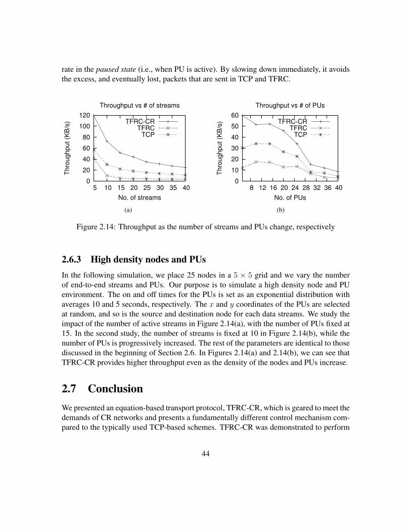
rate in the paused state (i.e., when PU is active). By slowing down immediately, it avoidsthe excess, and eventually lost, packets that are sent in TCP and TFRC.

0

20

40

60

80

100

120

5 10 15 20 25 30 35 40

Th

rou

gh

pu

t (K

B/s

)

No. of streams

Throughput vs # of streams

TFRC-CRTFRC

TCP

(a)

0

10

20

30

40

50

60

8 12 16 20 24 28 32 36 40

Th

rou

gh

pu

t (K

B/s

)

No. of PUs

Throughput vs # of PUs

TFRC-CRTFRC

TCP

(b)

Figure 2.14: Throughput as the number of streams and PUs change, respectively

2.6.3 High density nodes and PUsIn the following simulation, we place 25 nodes in a 5 × 5 grid and we vary the numberof end-to-end streams and PUs. Our purpose is to simulate a high density node and PUenvironment. The on and off times for the PUs is set as an exponential distribution withaverages 10 and 5 seconds, respectively. The x and y coordinates of the PUs are selectedat random, and so is the source and destination node for each data streams. We study theimpact of the number of active streams in Figure 2.14(a), with the number of PUs fixed at15. In the second study, the number of streams is fixed at 10 in Figure 2.14(b), while thenumber of PUs is progressively increased. The rest of the parameters are identical to thosediscussed in the beginning of Section 2.6. In Figures 2.14(a) and 2.14(b), we can see thatTFRC-CR provides higher throughput even as the density of the nodes and PUs increase.

2.7 ConclusionWe presented an equation-based transport protocol, TFRC-CR, which is geared to meet thedemands of CR networks and presents a fundamentally different control mechanism com-pared to the typically used TCP-based schemes. TFRC-CR was demonstrated to perform

44

significantly better than its classical counterparts TFRC and TCP with respect to both PUprotection and transmission efficiency in a dynamically changing spectrum environment.Our protocol does not assume any cross-layer feedback or input from intermediate nodes,which aligns it with the traditional end-to-end paradigm in the evolving space of transportlayer research for multihop CR networks.

45

Chapter 3

Accessing spectrum databases usinginterference alignment in vehicularcognitive radio networks

3.1 Problem overviewThe landmark FCC ruling in November 2011 in the US mandated the use of spectrumdatabases, with rules of access for stationary and mobile cognitive radio nodes, as well asthe consideration of specific capabilities such as geo-location [28]. These databases re-lease information on the spectrum usage in the vicinity of the requesting node, which mustbe periodically refreshed to maintain updated information. However, the FCC also allowsfor local spectrum sensing, though such unassisted and unilateral sensing by a node mustadhere to strict performance metrics. Identifying spatial regions or durations in which (i)the local sensing is likely to yield reliable and repeatable results (i.e., less random fluctua-tions on the signal imposed by the channel) and when (ii) accessing spectrum databases isa must, remains an open challenge.

In CR vehicular networks, where high bandwidth communication is required by fastmoving nodes, the exchange of spectrum information must be undertaken in the short-est possible extent of time [66]. This serves two important purposes: First, the spectrumknowledge remains current and relevant to the specific location a vehicle is currently sit-uated in, and second, given the large number of vehicles that traverse the road, it reducesthe channel usage time per vehicle. Thus, the wireless spectrum is more efficiently utilizedeven during the spectrum querying process, mitigating the risk of congesting this channelused for disseminating the spectrum queries.

The work described in this chapter is focused on answering the following two ques-

46

tions: How and when must a node rely on spectrum databases vs. relying on self-generatedmeasurements? When spectrum database query is the only solution, how do we ensure thatthe exchange of a large number of information and control feedback between the neigh-boring base stations (BSs) and the querying nodes is accomplished in minimum possibletime? To address the above concerns, we make the following contributions in this chapter:

3.1.1 Exploring signal correlation between 2G and TV channelsSignals from transmitters that are located in nearby areas are likely to experience a strongsimilarity in coarse channel behavior, owing to the common set of reflection, absorptioncausing objects and the large-scale path loss. We explore an interesting concept throughan experimental study, where we establish that at certain locations, the behavior of thereceived signal strength in cellular channels can be used to predict the accuracy of spec-trum sensing for certain channels in the TV whitespace. In some cases, the TV transmitterand one or more cellular transmitters (operating on totally different bands) are located neareach other, and when the signals from these two are received at a common location, we de-tect a strong correlation in the behavior of the Received Signal Strengh Indication (RSSI).Thus, any sudden change in the TV spectrum usage in such locations can be verified bycomparing with the corresponding fluctuations in the cellular channels. This provides anadditional layer of check and reduces mis-detection and false alarm. Of course, such aclose correlation occurs only for limited durations and at specific locations (based on therelative distances and the presence of these two different transmitter types), but it canpotentially offset costly spectrum database queries at these times.

3.1.2 Practical demonstration of interference alignment (IA)The method of interference alignment allows separation of the useful signals and the in-terference signals arriving at a node into orthogonal planes. In recent formulations, non-intuitive results were presented for two transmitters and two receivers, each of which is en-abled with two antenna modes, wherein four messages could be transmitted in three timeslots [67]. We further enhance this scenario with three concurrent transmitters, and extendthe basic formulations for a full duplex case with simultaneous transmission and reception.Specifically, we demonstrate how the resulting four transmissions and seven meaningfulmessage receptions (some of them at the intended node, some of them through overhear-ing) in three time slots are mapped into the case of multiple mobile CR vehicles seekingspectrum updates. To the best of our knowledge, we make the first scenario-specific useof the emerging technique of IA.

47

The rest of this chapter is organized as follows. We describe the related work and pro-vide background information on FCC database ruling in Section 4.2. Section 3.3 presentsthe network architecture and overview of the approach, followed by experimental findingsthat motivate our work in Section 3.4. The database querying strategy exploiting the corre-lation among TV whitespace and 2G spectrum, as well as the IA setup for efficient channelaccess, is given in Section 3.5. We undertake comprehensive performance evaluation inSection 3.6, and finally, conclude in Section 3.7.

3.2 Related Work

3.2.1 Cognitive radios and VANETsIn [68], the authors devise a spectrum sensing framework for CR enabled vehicles thatsend the data to roadside units or a base station (BS), which in turn forwards the data to aprocessing unit. The processing unit then infers which channels the vehicles are allowedto use based on the aggregate sensing information, and finally schedules this informationto be broadcasted to passing vehicles alongside. Belief propagation techniques are usedin [69], where vehicles combine different observations from surrounding vehicles, andspatial correlation is used to decide on channel availability. In [70], a framework for co-ordinated spectrum sensing method is proposed in the absence of any BS or a roadsidestatic base station. Instead, some vehicles are temporarily assigned the role of a “master”vehicle that coordinates the sensing and schedules the transmission activity of surroundingvehicles. In [71], a cooperative sensing framework called Cog-V2V is devised, where eachnode aggregates information it receives from surrounding vehicles to determine whichchannel to use in the current and future locations alongside the vehicles’ path. In a studyof a different nature, [72] analyzes a major interstate freeway in the state of Massachusetts(I-90) for free spectrum availability along its length. The authors argue for a use of acentralized database that vehicles can use to access the free spectrum information. An al-gorithm is also proposed on how to reliably populate such a database based on the sensingmeasurements obtained along the I-90 interstate.

3.2.2 Interference Alignment and Full-duplex wireless communica-tion

Few works exist that demonstrate real-time implementation of IA ever since the authorsof [42] wrote the first theoretical and practical scheme in IA. In [73], the authors developan improvement to the IA scheme called Blind IA where no previous Channel State Infor-

48

Protocol Use DB Distributed Use IA Improve sensing No precise chan.assignment

Ref [68] ✓

Ref [69] ✓ ✓ ✓

Ref [70] ✓ ✓

Ref [71] ✓ ✓ ✓

Ref [72] ✓ ✓

Proposed work ✓ ✓ ✓ ✓ ✓

Table 3.1: Comparison between our architecture and related works

mation (CSI) knowledge is required to achieve IA. This is in contrast to previous workswhere a use of offline calculations or a backchannel connection (e.g. ethernet) is used toexchange information among participating nodes to achieve IA [74].In [67], the authors present the first real-time implementation of blind IA based on a 2x2model. Similarly, [75] devise a way for wireless antennas to operate in full-duplex modewhere transmitters and receivers work concurrently using antenna separation and cancel-lation techniques. [76] further improved the full-duplex techniques by using Balun cancel-lation that has no bandwidth constraint, requires only two antennas, and does not requiremanual tuning, contrary to the assumptions made in [75]. In addition, they have alsoprovided the first MAC layer protocol for Full-duplex wireless communication.

Different from above, our work aims at sharing spectrum sensing correlation resultsbetween two different TV and cellular channels among nodes to improve the accuracy oflocal sensing. This is in contrast to previous works where nodes cooperate to choose acertain channel for communication. We also offer, to the best of our knowledge, the firstreal world scenario usage of IA in combination with full-duplex technologies by extendingthe scheme to allocate three transmitters that exchange four messages in three time slots.The combination of both technologies allow for an accurate, cost effective and efficientutilization of TV whitespace channels using both database management and local sensing.

Table 3.1 shows a comparison between our proposed architecture in relation to theaforementioned works.

3.3 Network Architecture and OverviewThe overall network architecture and usage scenario of our approach is shown in Fig-ure 3.1. A and B are two fixed BSs that have access to the spectrum database. Each BS

49

CD A B

dx

a cx

a

cx

b

d(x )

c

d(x )

a

d(x )

c

dx

c

Figure 3.1: Network architecture with two BSs A and B that have spectrum databaseaccess, and two vehicles C and D moving from left-right in a horizontal plane

can only provide reliable readings in a limited extent of space, shown by the boundarylines separating them. Each query to the database incurs a finite cost. CR enabled vehiclesmove along a straight line path from left-right, and two such nodes are indicated by C andD.• New incoming vehicle D: Node D enters a new region serviced by A. At this junction,BS A sends message xd

a which includes BS A’s ID, coordinates and transmission power.Node D becomes aware of this BS and may use it for future database querying requests.This beacon message xd

a is also overheard by BS B (more on that in the next section).• Fixed BS A and B: BS A sends its beacon information to D (xd

a) which D may useto query for the upcoming journey through the region served by A. xd

a includes A’s ID,coordinates and transmission power, which is also overhead by BS B. This informationcan be used, for example, so that the BSs minimize the overlap region of their coveragearea by dynamically adapting and coordinating their transmission power. As per the FCCruling, a mobile node operating in Mode II must request a new set of spectrum availabilityreadings after moving 100 m from its initial query point, or within a minute, whicheveroccurs earlier. Thus, a vehicle that has moved further into A’s territory (shown by vehicleC) beyond the first 100 m, must re-obtain the spectrum usage information. Vehicle Csends a preamble to synchronize the BSs in range and to request a new spectrum availabil-ity information. BS A sends this information (xc

a) which contains spectrum informationfor the remainder of the journey in A’s region. At the same time, BS B, which is alsosynchronized due to hearing the message preamble from C, provides the spectrum usage

50

(xcb) to vehicle C, as it is likely to enter B’s new service area next.

• Vehicle C within BS A’s service region: The decisions taken by vehicle C, and the subse-quent messaging that follows forms the core contribution of our work. C first determinesif there exists correlation among the 2G spectrum and TV whitespace using experimentaldata (Section 3.4), and if so, sends out a broadcast (xd

c) mainly intended for the incomingvehicle D. A high degree of correlation implies that the cellular channel can be a reliablemetric to quantify the likelihood of sensing errors. This message (xd

c) is also overheard byboth BSs A and B. This overheard message indicates which channels are correlated andtherefore can be used for future spectrum query replies. For example, a BS can prioritizethe usage of vacant channels that it knows vehicles on the road are not using (due to theabsence of any overheard correlation information by the BS). In turn, when D reaches thelocation currently occupied by C, it undertakes local spectrum sensing using the cellularand TV signal correlation (Section 3.5.1). If vehicle C’s measurements indicate that aspectrum update is necessary, then it issues a preamble similarly to vehicle C previouslyand both the BSs send the updated query information to vehicle D. The IA approach (Sec-tion 3.5.3) ensures that all the message exchanges involving vehicle C and the BSs arecompleted in fewer slots that the number of messages.

This cycle repeats as vehicles move in a straight line path, ensuring reduced spectrumupdate overhead and improved local sensing capability.

3.4 Experimental study of Correlation between 2G andTV Channels

To study the correlation between the RSSI in the cellular 2G frequencies and the TVchannels, we gathered a comprehensive set of measurements in the city of Boston over thespan of one month.

3.4.1 Experimental SetupWe used two devices to collect data simultaneously: a Universal Software Radio Platform(USRP) was used to sense the digital TV channels 21− 51 [77], and an Android SamsungGalaxy S3 smartphone was used to gather the following information: (i) RSSI valuesof nearby 2G cellular towers, (ii) current GPS coordinates, and (iii) the true TV spectrumavailability queried at 60 s intervals. We used Spectrum Bridge [34] by writing an Androidapplication that directly accessed their proprietary APIs to return the available/occupiedchannels and the signal strengths in the area of study. These devices were placed in acar, and the actual path traversed is shown in Figure 3.2(a). The path progresses along a

51

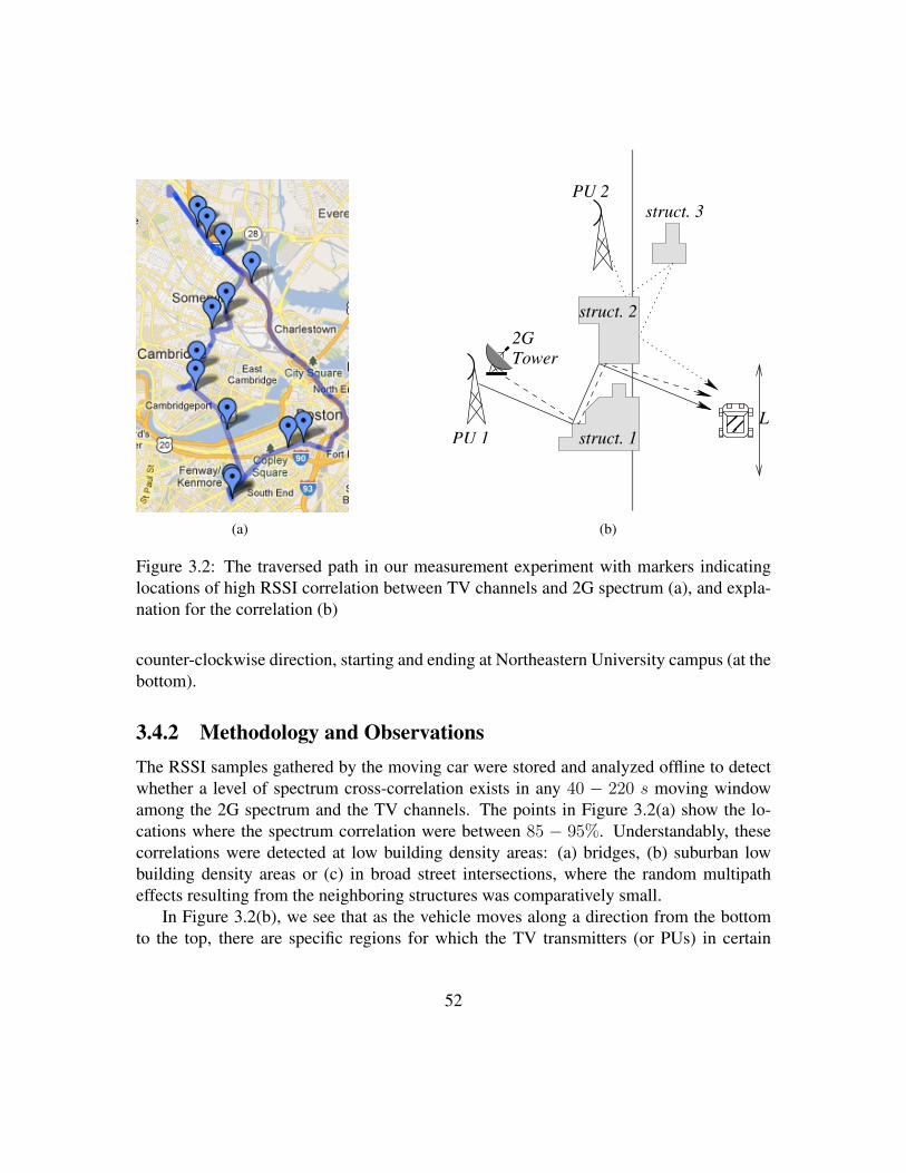
(a)

struct. 1PU 1

2G

Tower

PU 2

L

struct. 3

struct. 2

(b)

Figure 3.2: The traversed path in our measurement experiment with markers indicatinglocations of high RSSI correlation between TV channels and 2G spectrum (a), and expla-nation for the correlation (b)

counter-clockwise direction, starting and ending at Northeastern University campus (at thebottom).

3.4.2 Methodology and ObservationsThe RSSI samples gathered by the moving car were stored and analyzed offline to detectwhether a level of spectrum cross-correlation exists in any 40 − 220 s moving windowamong the 2G spectrum and the TV channels. The points in Figure 3.2(a) show the lo-cations where the spectrum correlation were between 85 − 95%. Understandably, thesecorrelations were detected at low building density areas: (a) bridges, (b) suburban lowbuilding density areas or (c) in broad street intersections, where the random multipatheffects resulting from the neighboring structures was comparatively small.

In Figure 3.2(b), we see that as the vehicle moves along a direction from the bottomto the top, there are specific regions for which the TV transmitters (or PUs) in certain

52

channels and the 2G spectrum towers are nearby, and their respective signals follow asomewhat similar propagation path. This scenario exists for PU1 and the 2G tower. At thistime, the signal from PU2, on a different TV channel, encounters an altogether differentmultipath environment. Thus, the signal fluctuations between 2G and PU1 towers arelikely to be correlated in a small window of the traversal path, shown by L, and totallyuncorrelated at other times when the structural neighborhood changes. Thus, on observingsudden changes in the subset of highly correlated TV channels and matching these changeswith the channel behavior of the 2G spectrum, the CR vehicle can identify if these arecaused by multipath effects or due to PU activity.

Figure 3.3 shows a randomly selected location point with two RSSI measurementsplotted against time, one from a 2G cellular tower and the other from channel number46 in the TV band, with intervals where strong correlation exist. The upper plot is formeasurements through the Android phone (i.e., measuring signals in the 2G spectrum)and the bottom one is from the USRP (i.e., in the TV channel). A moving average filterwith a set span 11 was applied to both RSSI values for smoothening before calculating thecorrelation. The correlation is obtained using the crosscorr function which is explainedby Equation 3.1. In this equation, f ∗ denotes the complex conjugate of f and n is the lagof one set relative to the other. We use a default lag of n = 20 (i.e. from −10 to 10) andevaluate max(f � g) as our maximum spectrum-correlation value. We see in Figure 3.3that the shaded time interval has 87% correlation while intervals immediately next to thissegment are highly uncorrelated: the spectrum-correlation yielded −22% and −44% forthese time durations before and after the shaded region, respectively.

(f � g)[n] =∞�

m=−∞f ∗[m] g[n+m] (3.1)

3.4.3 Motivation for Proposed ResearchIn our proposed method, for certain locations and TV channels for which a strong corre-lation exists with the 2G spectrum, the CR vehicle may not require additional spectrumdatabase updates to infer PU activity in these specific TV channels. Instead it may rely onlocal spectrum sensing alone, as for these channels it can track and attribute the cause ofrapid signal fluctuations, thereby lowering the chance of false alarm and missed detection.

A vehicle that already has access to 2G RSSI values (effectively operating in ModeII) may be able query the spectrum database directly without the need of a roadside basestation or to perform local sensing. However, this is not always possible or optimal dueto multiple factors: (a) the phone observes the RSSI values but does not access the Inter-net (e.g. when roaming). Moreover, a phone’s service provider represents only a subset

53

Figure 3.3: Spectrum correlation between one TV channel band and one 2G radio towerRSSI values

of the total RSSI values obtained, while a significant portion of the measurement data isgathered from towers that the phone cannot legitimately connect to (i.e. different HSPAmobile carriers), (b) having access to roadside base stations or local sensing, as opposedto querying the database directly, will save in the total overhead over the Internet giventhat a BS needs to query the database once every 24 hour period. The BS can then me-diate and share that information with passing vehicles saving on total traffic directed tothe centralized database, (c) the latency to retrieve such spectrum information is reducedbecause the BS is much closer to the vehicles than an online database, and (d) given thatthe information is retrieved from the BS which queries the database once and then sharesit at a fraction of a cost, the total cost per query incurred by each vehicle is also reduced.

3.5 Optimal Database Querying StrategyUsing the network architecture described in Fig 3.1, we discuss in this section how anode decides whether spectrum database or local sensing needs to be undertaken, how toimprove the local sensing capability, and undertake message transfers with reduced controloverhead.

54

Time

RS

SI

Threshold

Threshold

Case I Case II

Case IVCase III

Figure 3.4: Four different types of RSSI readings performed by sensing

PU Present PU Absent

2G<TH 2G<TH 2G<TH2G>TH 2G>TH 2G>TH

1 2 34

WS>TH WS<TH WS>TH WS<TH

5

67

Figure 3.5: Decision tree of the cognitive radio node. Solid lines indicate a possibleoutcome while the dotted lines indicate the impossible ones

55

3.5.1 Exploiting Correlation between 2G and TV WhitespaceNode C collects the RSSI values of the 2G and whitespace towers spectrum, and analyzesit to determine if a high correlation exists between any pair of TV channels with those inthe 2G band. We describe the four cases below that demonstrate the types of readings thatC may obtain at any given point. The four cases are shown in Figure 3.4.• Case I is when a vehicle reads RSSI values that all surpass a certain sensing thresholdλ [78] on average.• Case II is when the average drops below that threshold due to significant fading.• Case III represents very low RSSI readings, which is the case for vacant channels. TheseRSSI readings are well below the threshold.• Case IV occurs when the average RSSI value is above the threshold, but the channel isreally vacant. Case IV’s outcome, however, can be minimized because contrary to currentdetection schemes that have a probability of false alarm rate [78–80] due to uncertainnoise power knowledge, in our proposed architecture, nodes can have perfect noise powerknowledge by studying the RSSI values of channels that are known to be vacant by thedatabase and setting the threshold to a value above the highest observed floor noise RSSIvalue. After minimizing the probability of false alarm in Case IV, vehicle C will haveto make a decision based on which of the remaining three cases of RSSI readings it iscurrently observing.

Vehicle C uses the observed RSSI values (in the 2G spectrum and the TV whitespace),as well as the energy detection based sensing threshold λ to infer whether a PU exists ornot, or whether the correlation information leads to indeterministic results. We use Fig-ure 3.5 to explain the possible scenarios using the decision pathways indicated by numbersat the end points in the figure. The following numerical list correspond to these numbers.Note that this decision logic is used after correlation is detected by C between the 2G andthe TV whitespace (WS) RSSI signals. The dotted lines indicate a state that is not feasible,while the solid pathways indicate a possible outcome:

1. WS RSSI > λ and 2G RSSI > λ: this indicates that the PU is currently occu-pying the channel because a correlation exists, and both RSSI values are above thethreshold λ.

2. WS RSSI > λ and 2G RSSI < λ: this scenario is not feasible because the 2Gtowers don’t have an on and off time and should remain constantly on at this location.Therefore if a correlation existed between this pair previously, this outcome is notpossible. If the 2G network is not present, then we expect the WS channel to also bevacant due to their previous correlation but this isn’t the case. The node must querythe database if it wishes to use this whitespace channel.

56

3. WS RSSI < λ and 2GRSSI > λ: this outcome indicates that a PU is not present;the two signals were previously correlated (and correlation only happens when bothchannels are not vacant), if the 2G signal is still occupied while the WS signal isnot, then this indicates that the PU is not present and the node may use this channelto transmit data. These two channels have a high correlation therefore if fading,shadowing or multipath effects exists, it will affect both of the channels and not justone of them. This is not a possible outcome if the PU is present.

4. WS RSSI < λ and 2G RSSI < λ: this is a possible outcome if the PU is present.The two correlated channels are below the threshold λ which indicates a possiblefading/shadowing/multipath effect that is affecting both channels. The read RSSIvalues are below the threshold but we know from previous correlation that the twochannels exhibit the same effects.

5. WS RSSI > λ: From our experiment results, if WS RSSI values are above thethreshold λ, then this indicates that the PU is present. Therefore this is not a possibleoutcome.

6. WS RSSI < λ and 2G RSSI > λ: this is a possible outcome, see (3) above.

7. WS RSSI < λ and 2G RSSI < λ: this is not a possible outcome because if thetwo channels are correlated, then the absence of the 2G RSSI network indicates thepresence of channel effects (fading/shadowing/multipath) that is exhibited on bothchannels, and therefore the PU is still occupying the channel.

3.5.2 Database Query or Local Sensing DecisionIn this section, we explain the querying process for a snapshot of the vehicles currentlyin the network, and shown in Figure 3.1. We show how the database querying is ac-complished by vehicle C, resulting with low traffic on the channel. We then extend thediscussion for vehicle D, and then finally, for any other general vehicle along the road.• Case for Vehicle C: In this case, vehicle C follows the steps outlined in Figure 3.6 to de-termine if it is able to come to a conclusion about the PU activity using the correlation andRSSI measurements. As vehicle C enters a new region, it checks to see if there is any priorknowledge of correlation between TV whitespace and 2G spectrum at its present location.If no (the decision flow moves along the right arm of the flowchart), it issues a spectrumquery to the nearest BS. At this stage it is in a position to measure the signal correlationitself, and inform other vehicles in the downstream chain. If a spectrum-correlation isfound, it broadcasts that information to these vehicles, including node D. If no correlation

57

is detected, it simply uses spectrum information from the database, and concludes the al-gorithm. Please note that the Query Database and the Find Correlation blocks can happensimultaneously; this key fact will be used in the subsequent section when querying thedatabase and transmitting to the downstream vehicle happens simultaneously via IA.• Case for Vehicle D: We describe this case for vehicle D using the left arm traversal ofthe decision logic in Figure 3.6. We assume that it received prior confirmation of spectrumcorrelation at its present location (say, by vehicle C). It then uses the reasoning describedin Section 3.5.1 to determine PU presence. First, it checks if the TV whitespace (WS)RSSI readings are below the threshold. If so, it checks whether the 2G RSSI readingsare also below the threshold. If both conditions are true, then it concludes that the PUis present. It arrives at this somewhat nonintuitive result as (i) the prior vehicle verifiedcorrelation exists, (ii) the 2G spectrum has beacon signals that are always present at setintervals in time, and (iii) it does not detect the 2G beacons, possibly lost due to multipathand fading, which indicates similar trends in the TV whitespace. On the other hand, if the2G RSSI values are above the threshold, then (see path 6 in Figure 3.5) we determine thatthe PU is absent, and D may use that channel for data communication.

If, however, the whitespace RSSI is above the threshold λ which indicates the pres-ence of the PU, vehicle D completes the algorithm by moving to the right arm of thedecision flow, i.e., it issues a query to the database. The rest of the steps follow exactly theprocedure for vehicle C described above.

The description of the steps for this network snapshot are applicable for any vehiclein the network. The overall actions of the vehicles along the entire length of the roadallows each vehicle to extrapolate correlation information and hence, serve as the sourceof spectrum correlation information for the remaining downstream vehicles.

3.5.3 Spectrum Updates using Interference AlignmentThe overall aim of the database access phase, when it occurs, is to allow all the transmis-sions and packet exchanges to be completed in exactly three time slots. This results in aremarkable efficiency of the channel usage. The modification to the classical IA schemethat is leveraged for this purpose is described next.

Interference alignment places the interfering signals along vectors oriented orthogonalto those of the useful signal [42]. It achieves this by allowing the receiver to switch antennamodes according to a pre-set pattern. The antenna mode can be altered by changing theantenna response parameters, reducing the height, or as we suggest in our case, simplyuse antenna 1 or 2, when the receiver needs to be in mode 1 or 2, respectively. Thus, IAdemonstrates much improved resilience to signal losses by not attempting to cancel or limitthe interference level at its location, which requires extensive transmitter side information.

58

Enter a NewRegion

End Sending

Yes

NoCorrelationExist?

Yes

No

WSRSSI > TH

Yes

No2GRSSI > TH

Yes

NoCorrelationExist?

QueryDatabase

FindCorrelation

BroadcastCorrelation

PU Present

PU Present

PU Absent

Figure 3.6: Sensing vs. Querying decision flow chart

59

2

11h

ac

12h

ac

11h

ad

12h

ad

12h

bc

11h

bc

22h

cd

B

A

D

C

1

2

1

11

2

2

Figure 3.7: Interference alignment with three transmitters (A, B, C) and two intendedreceivers (C, D)

Our extension to the 2x2 blind model of IA proposed in [67] is based on two importantconsiderations. First, we use a full duplex radio that can simultaneously transmit andreceive, though it has only one transmitter and receive chain, respectively. Off the shelfUSRP radios can be adapted to support this full duplex operation [75, 76]. Secondly, wedepart from the traditional model of a cleanly separated set of transmitters and receivers.Instead, in our case, one of the receivers (vehicle C) switches its role into a transmitter tosend a message to the second receiver (i.e., the downstream vehicle D). The individualalignment equations based on the received packets are described below for each node, andthe channel gains for the unidirectional transmissions are depicted in Fig 3.7.

Transmitter/Receiver- Vehicle C

CR Vehicle C changes its mode in the pattern 1−2−1, as indicated by switching betweenthe antennae 1 and 2. It subtracts the third equation from the first to get two unknowns intwo variables, by eliminating xd

a, which is the message destined for D. The resulting set oflinear equations can be solved to obtain xc

a and xcb, respectively. These unknowns represent

the spectrum database information C requested from A, and B for the subsequent journeytowards B’s control region. In the last transmission slot, C transmits its assessment of thefeasibility of spectrum sensing to D, using the transmit antenna 2. This message, xd

c , isalso overheard by the BSs A and B, which as we noted previously in Section 3.3, can beused for different quality of service channel prioritization in all subsequent queries.

Receiver- Vehicle D

CR Vehicle D subtracts the second equation from the first, for which it was in the samemode 1. This leaves the only unknown xd

a, which is the beacon information that A intendsto supply to D as it enters for the first time in its control region. This value is then sub-

60

AntennaNode C

Rx Tx

1 z[c](1) = (xca + xd

a)h11ac + (xc

b)h11bc

2 z[c](2) = (xca)h

12ac + (xc

b)h12bc

1 2 z[c](3) = (xda)h

11ac

Table 3.2: Interference alignment equations for node C

tracted from equation 3 to obtain xdc , the transmitted message from CR vehicle C to D.

Vehicle D’s transmitter antenna remains unused throughout the process.

AntennaNode D

Rx Tx

1 z[d](1) = (xca + xd

a)h11ad + (xc

b)h11bd

1 z[d](2) = (xca)h

11ad + (xc

b)h11bd

2 z[d](3) = (xda)h

12ad + (xd

c)h22cd

Table 3.3: Interference alignment equations for node D

Transmitter- BS A

BS A hears the transmissions from the neighboring BS B in the first two slots, and thetransmission from vehicle C to D in the final slot xd

c . This last message also informs BSA what channels vehicle C found to be correlated and may use that information for sub-sequent queries in, for example, optimizing quality of service. While A does not switchoperational modes, it does rely on the full duplex ability to continuously transmit on an-tenna 1 and receive on antenna 2.

In the first slot, it transmits a summation of the messages xca + xd

a to both the vehicles,while in the second slot, it only transmits xc

a to vehicle C. These messages are received bythe adjoining vehicles and BS B in the first two slots, respectively, subject to the channelgains from A to them.

61

AntennaNode A

Rx Tx

2 1 z[a](1) = (xcb)h

12ba

2 1 z[a](2) = (xcb)h

12ba

2 1 z[a](3) = (xdc)h

22ca

Table 3.4: Interference alignment equations for node A

Transmitter- BS B

The operation of BS B is very similar to that of C. Subtracting the second equation fromthe first returns the message xd

a sent to D from A. This is, in turn, substituted in equation3, to obtain xd

c , which informs B what channels vehicle C found to be correlated and mayuse that to improve subsequent queries’ quality of service.

AntennaNode B

Rx Tx

2 1 z[b](1) = (xca + xd

a)h12ab

2 1 z[b](2) = (xca)h

12ab

2 z[b](3) = (xda)h

12ab + (xd

c)h22cb

Table 3.5: Interference alignment equations for node B

In summary, the information exchange equations are carefully constructed using IA,while ensuring that the preference for local sensing or database updates is correctly com-municated to the network entities.

3.6 Performance EvaluationIn this section, we first provide trace-driven simulation studies to demonstrate the feasi-bility of exploiting the spectrum correlation approach described in Section 3.6. Then, weprovide quantitative results on the efficiency of the channel utilization by using the IAscheme from Section 3.5.3 through a simulation study in MATLAB.

62

0 0.2 0.4 0.6 0.8 1 1.2 1.4 1.6 1.8 2 2.2

x 104

0.5

1

1.5

2

x 105

Time (seconds)

Nu

mb

er

of

Sp

ectr

um

−C

orr

ela

tio

n P

oin

ts

70% cross−corr

75% cross−corr

80% cross−corr

85% cross−corr

Figure 3.8: Number of spectrum-correlation points as the time of the experiment increases

3.6.1 Improvements due to spectrum correlation exploitationWe use traces from the experimental setup described in Section 3.4, where a USRP radiois placed inside a moving vehicle. The Android phone accesses the 2G spectrum, main-tains a history of the path traveled via the in-built GPS capability, as well as queries theSpectrum Bridge Inc. database through software APIs every 100m traversal, or when 60selapse, whichever is earlier. As a subsequent check, all measured sensing results obtainedvia energy detection through the USRP are validated with offline verification through thedatabase, at the end of the experiment. A subsequent trailing vehicle may schedule its ownquery, unless the vehicle ahead transmits a beacon that informs it to cancel the databasequery and rely on local sensing, using the procedure adapted from Section 3.5. The ob-served signal fluctuations in the 2G spectrum as well as the TV whitespace are saved ina laptop computer and correlations are calculated via a continuously running MATLABprogram.

Number of spectrum correlation points

Figure 3.8 shows the number of spectrum-correlation points as the vehicle moves alongthe map shown in Fig 3.2(a). In this figure, we can see that the number of these pointsis higher when the correlation level is set at 70%, as compared to 85%, by about 4 times.This demonstrates the trade-off that exists between higher accuracy (imposed by highercorrelation demands) between the 2G spectrum and TV whitespace, and total number ofcorrelation points where this approach can actually be used.

63

2000 4000 6000 8000 10000 12000 14000 160000

20

40

60

80

100

120

140

Distance (in meters)

Nu

mb

er

of

Qu

erie

s

None

85% cross−corr

90% cross−corr

95% cross−corr

Figure 3.9: Number of queries for various spectrum correlation percentages

Number of queries

We list the total number of database queries that a vehicle engages in the path that wastraversed to collect the spectrum information in Figure 3.2(a). As the distance traversedincreases, the number of queries that have to be performed also increase. In Figure 3.9,we plot the number of queries that are undertaken by the CR vehicle if no spectrum cor-relation information is leveraged, as opposed to when it utilizes the spectrum correlationinformation to reduce the number of direct queries. Lower the allowed spectrum correla-tion percentage, the less the number of queries that the vehicle will undertake. In the caseof correlation level set to 70%, the vehicle only needs to query the database 108 times,instead of 140 without our proposed scheme. This results in a saving of up to 23%. Thisnumber can be easily scaled with appropriate multipliers, such as the monetary cost ofspectrum usage time imposed by carriers, the channel utilization, resulting data conges-tion, among others to obtain tangible impacts of reducing the number of database queries.

Accuracy

In Figure 3.10, we plot the probability of error with (P xerr) and without (P c

err) our proposedscheme where

Perr =Number of times the query resulted in mis-detection

total number of queries(3.2)

We first calculate P cerr by assuming Rayleigh fading over a period of time for the gath-

ered RSSI readings, to check whether the average RSSI values obtained over the sensingtime ts are above or below the RSSI threshold λ. Here, we chose ts = 0.022s and λ was

64

Figure 3.10: Accuracy of sensing

empirically observed over the total simulation time [78] to be −0.5 (amplitude dB). Wethen calculate the fraction of times that the average RSSI value is below the threshold overthe total number of sensing intervals to give us the classical energy detection probabilityof error P c

err. This is in turn plotted against P xerr:

P xerrj

= (1− xj

X)× P c

errj(3.3)

where xj is the number of spectrum correlation matches that occur at speed j, and X is thetotal number of such correlations obtained over the entire experimental duration. One canobserve that the probability of error decreases as the speed of the moving vehicle increasesfor both the classical energy detection and the correlation based approach. However, theerror in the latter is always less at all the measured speeds. This is because the RSSI maystay below the threshold for longer periods of time when the speed is slower, resulting inthe sensing errors when ts = 0.022s [78].

3.6.2 Improvements through interference alignmentIn this section, we simulate the scenario in Figure 3.1 where the entire distance traversedis 2 km and the BSs A and B are located at distance 500m and 1500m, respectively withthe coverage radius of each BS set to 500m. We vary the inter-arrival rate of vehicles that

65

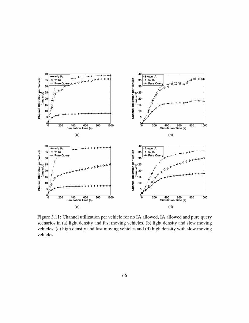
0 200 400 600 800 10000

5

10

15

20

25

30

35

40

Simulation Time (s)

Ch

an

nel U

tilizati

on

per

Veh

icle

(tim

e s

lot)

w/o IA

w/ IA

Pure Query

(a)

0 200 400 600 800 10000

5

10

15

20

25

30

35

40

Simulation Time (s)

Ch

an

nel U

tilizati

on

per

Veh

icle

(tim

e s

lot)

w/o IA

w/ IA

Pure Query

(b)

0 200 400 600 800 10000

5

10

15

20

25

30

35

40

Simulation Time (s)

Ch

an

nel U

tilizati

on

per

Veh

icle

(tim

e s

lot)

w/o IA

w/ IA

Pure Query

(c)

0 200 400 600 800 10000

5

10

15

20

25

30

35

40

Simulation Time (s)

Ch

an

nel U

tilizati

on

per

Veh

icle

(tim

e s

lot)

w/o IA

w/ IA

Pure Query

(d)

Figure 3.11: Channel utilization per vehicle for no IA allowed, IA allowed and pure queryscenarios in (a) light density and fast moving vehicles, (b) light density and slow movingvehicles, (c) high density and fast moving vehicles and (d) high density with slow movingvehicles

66

arrive from left to right in the figure (read vehicle density) and the vehicle speed and deter-mine the performance gains in channel utilization and number of queries. We compare theperformance of different scenarios: (a) Pure query: in this case, vehicles do not leverageany spectrum correlation information. Vehicles entering will query the database whenever60 s has elapsed or 100 m was traversed. No carrier-sensing algorithm is implementedhere, so the queries may collide causing interference. (b) CSMA: in CSMA, vehiclesback-off when a collision is detected based on 802.11 standards. (c) Without IA (w/o IA).This scenario has vehicles using spectrum correlation information to save database querycosts but does not exploit IA for channel utilization gains and (d) with IA (w/ IA) wherevehicles send data using IA after exploiting any spectrum-correlation information. In allsimulations, we use a real-world segment of the RSSI readings that we obtained in ourMarch 2011 experiment (See section 3.4).

Channel utilization

Figure 3.11 shows a comparison of channel utilization per vehicle (time slots) in variousspeed and density scenarios as the simulation is run for a duration of 1000 s. The resultsare averaged over 20 simulation runs. There are a number of interesting facts that can bederived from the four figures: (a) When speed is increased, the channel utilization is im-proved through IA because a vehicle can obtain future spectrum information from towerB at the same instance it is also obtaining it from A for the rest of the duration in A (SeeSection 3.5.3 and 3.6), while in the slower scenarios, the vehicles have expired spectruminformation which requires them to re-query the database and hence incur higher chan-nel utilization. (b) When density increases, without IA (w/o IA) scheme is significantlyimproved over pure query. This is because having more cars in the scenario leads to bet-ter chances of sharing (and exploiting) spectrum-correlation information and hence, lesschannel utilization. (c) In all scenarios, IA outperforms both pure query and without IA.

In Figure 3.12(a), we vary the vehicle density (inter-arrival rate) while keeping thevelocity constant. Conversely, in Figure 3.12(b), we fix the vehicle density and vary thespeed. We compare CSMA with pure query, no IA information leveraged, and full IA inthe global utilization of the channel. In both cases, the CSMA reaches channel saturationearly. This is because an increase in vehicle density and speed causes more collisions,leading to the channel being sensed for prolonged periods of time. We also see that whenwe increase the vehicle velocity in Figure 3.12(b), the IA scheme results in slower increasein total channel utilization than that of pure query and without IA. Since we keep theaverage distance between vehicles unchanged, increasing the speed results in an increaseof the number of cars entering the region at any given time and thus, in all cases totalchannel utilization increases. When we increase the vehicle density in Figure 3.12(a), we

67

10−3

10−2

10−1

100

0

2

4

6

8

10x 10

5

Vehicle Density (vehicles/m)

Ch

an

nel U

tilizati

on

(ti

me s

lot)

w/o IA

w/ IA

CSMA

Pure Query

(a)

5 10 15 20 25 300

2

4

6

8

10

12x 10

5

Vehicle Velocity (m/s)

Ch

an

nel U

tilizati

on

(ti

me s

lot)

w/o IA

w/ IA

CSMA

Pure Query

(b)

Figure 3.12: Channel utilization per vehicle (a) density and (b) velocity changes, respec-tively

see that CSMA attains maximum channel utilization before the three remaining schemes.Additionally, these competing schemes result in a faster increase in channel utilization asthe vehicle density grows, as compared to the scheme with IA.

Number of queries as the noise level changes

In Figure 3.13, we apply White Gaussian noise to the signals on the 2 km stretch of thesimulation with increasing SNRs. The plot shows that as the SNR increases, the numberof queries decreases. This is due to having more spectrum-correlation between the TVand 2G signals as the SNR increases leading to less reliance on the database to query forspectrum information.

3.7 ConclusionIn this chapter, we describe a new paradigm for spectrum database access, which allowsquerying the database only when needed. The resulting method exploits the correlationthat exists among two entirely different spectrum bands at specific locations, thereby im-proving the performance of local sensing and reducing the costs associated with repeateddatabase queries. Results reveal about 23% reduction of queries, making it attractive forpractical spectrum database deployments. In addition, we also explored a real-world in-terference alignment application that can reduce the control channel utilization. We fol-lowed this by simulation runs to verify the performance gains using this approach. This

68

Figure 3.13: Number of queries as the SNR increases

non-trivial approach can potentially open up a hitherto unexplored direction in spectrumsensing, and future work will be focused on building the protocol suite that enables quickand efficient exchange of spectrum data between the vehicles and the BSs.

69

Chapter 4

A cognitive radio module for thenetwork simulator 3

4.1 Problem overviewNetworking engineers and researchers contributing in the emerging area of cognitive ra-dio researchers face uphill challenges when testing a new concept, given the challengingenvironment in which these networks operate. The CRs must opportunistically determinewhich licensed channels are available and make use of this spectrum before the licenseduser reclaims it. Accurate protocol operation is critical, as any prolonged use of the chan-nel raises concerns of interfering with the activities of the licensed users. This concerndirectly translates to meticulous testing of the protocol or networking concept in a con-trolled environment. Given the uphill costs of purchasing multiple software defined radiosthat serve as the hardware building blocks of the CR network, and the time investment iswriting and deploying code in them, computer simulation often becomes the methodologyof choice.

While several commercial simulators exist, such as OPNET [43], which can capablysimulate heterogenous networks, our focus in this work remains on affecting improve-ments to open-source simulators. The main challenges in such environment are as follows:

• CR protocols are generally cross-layered. Any change in one layer, such as spectrumsensing duration at the physical layer (PHY), has direct impact on the decisionsmade in the upper layers of the protocol stack, requiring extensive code changesthroughout the stack.

• The testing time increases dramatically with the complexity of the protocol. Owingto the large number of variables that can be controlled, identifying the dominating

70

factor that impacts the environment to the greatest possible extent may force largenumber of trial runs.

• The inter-dependence of the protocol layers requires network architects to imple-ment more than one layer. For e.g., spectrum sensing at the PHY can impact theTCP throughout and its interpretation of congestion. Thus, the expertise required tosimulate CR networks effectively is more than conventional wireless networks.

• New functions unique to the area of CR, such as spectrum sensing, spectrum hand-off and licensed or primary user detection need to be embedded in the simulator.

This chapter is focused on providing the first cognitive radio extension to the networksimulator 3 [44] or ns-3, which is a discrete event driven simulator. This simulator ispoised to replace the widely popular predecessor, network simulator 2 or ns-2. Ns-3 offersseveral advantages over ns-2, including: (i) it has a new core written in C++, (ii) it is gearedfor wireless communications, (iii) it has an organized modular architecture that is expand-able, (iv) it includes intuitive and extensive documentation via the html Doxygen [45]interface, and (v) the same ns-3 code can be easily adapted to work in real devices [44].

Despite the clear superiority of this new simulation platform, ns-3 lacks implementa-tion support for CR networks. To introduce this capability, several changes are required invarious network layers in ns-3. For example, a device needs multiple wireless interfacesto transmit, receive and negotiate with neighboring nodes. The PHY need to be able tosense and detect Pus, the medium access control (MAC) needs to decide and initiate hand-off to another available channel when a PU is detected, and the routing protocol needsto exchange the neighboring nodes’ current listening channel. Based on the recent FCCmandate [28] that requires CRs to use a centralized spectrum database, the simulator willhave to also incorporate such querying capabilities to identify the available channels usingthese databases.

Our main contribution is to fully realize the first CR extension for ns-3 that has thefollowing features:

• It provides CR capabilities at the different network layers such as sensing, PU de-tection, channel hand-off and decision making.

• It incorporates the ability to query a database to obtain PU activity results.

• It has the ability to simulate cognitive with non-cognitive legacy wireless nodes inone test environment.

• It includes seamless support for multi-channel and multi-radio node architectures.

71

Simulator Multi-interface Hand-off Cog and Non-Cog Query DB Extensible policies Ns-3CRCN [81] ✓ ✓

CogNS [82] ✓

[83] ✓ ✓ ✓ ✓

[84] ✓ ✓ ✓

CRAHN [85] ✓ ✓

CRE-NS3 ✓ ✓ ✓ ✓ ✓ ✓

Table 4.1: Comparison between CRE-NS3 and related works

• It provides new application programming interfaces (APIs) to expose the creationof these node-level and network-level features without advanced code changes. Itcomes with extensive documentation through Doxygen.

• It allows studying the overhead, performance, and comparison with an existing ex-tension of CR in ns-2.

• It is accompanied by the release of the full source code, with additional guides onhow to compile and run trial examples.

The rest of this chapter is organized as following: Section 4.2 discusses the existingnetwork simulators, and their utility in implementing work for CR networks. We describethe model of our proposed approach in detail in Section 4.3, followed by the proposedchanges to the networking layers in ns-3. Performance evaluation studies are presented inSection 4.4, and finally Section 4.5 concludes the chapter.

4.2 Related Work and BackgroundTo the best of our knowledge, no previous CR implementation exists for ns-3. There are,however, few modules for CR that has been built for other simulators. Cognitive RadioCognitive Network (CRCN) [81] provides a radio extension for ns-2. This simulationframework provides multi/single radio and multi-channel support per node. It providesAPIs that return information, such as the current noise or traffic conditions at a givenchannel, and provides a mechanism for channel hand-off. CogNS [82] provides anotherextension to ns-2. This module allows one network interface per node that is able tosense PU activity and defer to another free channel based on a proposed spectrum decisionalgorithm. Nodes created in this environment cannot incorporate multiple radios per node.[83] provides a CR simulation extension for OMNeT++ [86]. It provides support formultiple interfaces per node, and is focused on evaluating CR MAC layer protocols.

72

[84] is a simulator written in C++ for CR networks. The proposed simulator offers amodular approach that provides a full network layer stack. Because this work is not basedon a more popular platform that has been tested by the general networking community, thissimulator involves some overhead in porting the already known protocol stacks in chang-ing environments. For e.g., for a researcher interested in simulating CR networks withan alternate MAC, such as a different 802.11 standard, the effort required is prohibitive.As compared to this, other popular simulators such as OMNet++, ns-2 and ns-3 alreadyprovide a wider user-base and support community.

The work described in this chapter uses the ns-2 CRAHN extension in [85] as thestarting point. This earlier CR extension for ns-2 provides three network interfaces pernode; a control interface to exchange control information between neighboring nodes,a receiving and transmitting interface. The CR module also incorporates hand-off andsensing capabilities at the PHY and MAC layers. It provides for PU detection mechanismsbased on a PU activity model table that is loaded in the simulator a-priori. Our work, whilebased on this extension, has the following key differences: all the work that is proposed inthis chapter is based on the new ns-3 simulator, which (i) requires extensive code change,(ii) provides dynamically adjustable sensing/hand-off times that can be configured fromthe command line, (iii) is able to include cognitive and non-cognitive interfaces in onenode, and (iv) is able to mix cognitive and non-cognitive nodes in one test environment.The simulation extension we propose can also incorporate a larger number of cognitiveinterfaces and/or nodes compared with ns-2 (in the order of thousands). We also designa different simulation architecture, composed of a Spectrum Manager block that hides ormasks the inner CR API calls, leading to an organized modular approach.

Overall, our proposed extension provides easy access to the specialized CR function-alities compared to other existing simulators through APIs, offers flexible CR and non-CR nodes to coexist, and incorporates advanced abilities, such as querying the recentlymandated FCC database to infer PU activity. Our work aims at realizing a complete CRsimulation platform to save time and resources for CR researchers who are either forcedto write the entire CR software stack or embark on the costly enterprise of purchasingmultiple real devices.

Table 4.1 provides an overview of the comparison between our proposed ns-3 exten-sion, and the other approaches discussed in this section.

4.3 Ns-3 Simulator Model for CRIn this section, we present the architectural model of our proposed ns-3 simulator. We firstdescribe the building blocks of the extension, followed by an explanation of the needed

73

SpectrumSpectrum

Spectrum

Spectrum

Mobility

Sharing

Sensing

Decision

Environment

Radio

Channel

Capacity

TransmittedSignal

Primary UserDetection

Spectrum HoleDecisionRequest

SpectrumCharacterization

Figure 4.1: Cognitive cycle [1]

changes at various network layers for a given node.

4.3.1 Building blocks for the simulatorThe typical functions of the CR node, follow the essential stages of Spectrum Mobility,Spectrum Sharing, Spectrum Sensing and Spectrum Decision, as described in the cogni-tive cycle described in [1]. As seen in Figure 4.1, these operations may occur one afterthe other, moving the CR node from one operational stage to the next. We use a similarapproach to design the ns-3 simulator, by implementing each of these constituent blocksof the cognitive cycle, as shown in Figure 4.2. The spectrum management global blockserves as a black box to the other modules in ns-3. Different layers in the network simulatorkeep a reference to the Spectrum Manager instance and tie their cognitive functionality viaexposed APIs and hooked listeners. An example of such APIs are startSensing(),startHandoff(channel), isSpectrumFree(channel), alertNeighbors().

Internally, the Spectrum Manager block contains several submodules that map to thecognitive cycle, which are described next.

• Spectrum Sensing/Database Query. This block is responsible for checking whethera PU exists in a given channel within a specified period of time. It infers the PU ac-tivity from a static PU Database that is loaded before the simulation starts. Thissubmodule can be used to either (a) mimic sensing with a given probability of sens-ing error Perr, or (b) query an FCC approved database to determine the PU activity.The PU database that is loaded into the simulator is a text file that defines the num-ber of PUs, their current occupied channel, the transmission power to determine therange, and a list of on (PUon) and off (PUoff ) times. A researcher can create and

74

Figure 4.2: The main building blocks of the proposed extension

load this text file with any given PUon and PUoff distributions such as normal orexponential.

• Spectrum Decision. In this block, several policies are implemented. First, a policyin incorporated to determine whether a hand-off should be performed based on sens-ing/querying results. Second, a policy that determines to which channel a hand-offshould happen is written. Note that these policies are extensible: One can implementdifferent and independent policies, or extend the existing ones. A global repositoryis linked to this submodule which hosts current occupied channels by all CR nodesin the simulator. This can be used, for example, to determine the least occupiedchannel that a node should switch to to guarantee desired Quality-of-Service (QoS).

• Spectrum Mobility. This submodule initiates the hand-off protocol in the currentnode. It is tied directly to the PHY layer in the ns-3 node which will be discussedlater in Section 4.3.2.

• Spectrum Sharing. This submodule uses the built-in carrier sensing MAC 802 11standards in ns-3 to make sure that the available spectrum is shared in a collision-free manner between the CR nodes that chose to transmit on this same channel.

These sub-blocks are linked internally whenever a given API in the Spectrum Manager

75

block is invoked. For example, to initiate sensing, a researcher may invoke a call to thestartSensingAndSwitchIfNecessary() API from any arbitrary network layer.The Spectrum Sensing block will then initiate a look-up via the PU Database, call theSpectrum Decision block once sensing is performed. If the Spectrum Decision blockdecides to switch to a new free spectrum, it initiates a hand-off via a call to the SpectrumMobility block. The same network layer that invoked the call will then be notified via alistener once this cycle is completed and transmission can be resumed. This can be used,for instance, in a transport layer protocol where the transport protocol needs to determinewhen to resume the data flow [87].

4.3.2 Layer-specific modifications to ns-3In this section, we detail the needed changes to each layer of the protocol stack for a givenCR node in ns-3. Figure 4.3 depicts an overview of these changes. As can be seen, theproposed CR extension exposes several APIs and listeners to all the networking layers. Wealso make use of ns-3 tagging feature. The method to ‘tag’ a packet with some informationhelps to determine that packet’s internal routing in a given node, thereby avoiding thecostly overhead that would ensue if said information was to be integrated into the packet’sheader instead. More details on this feature and how it is used will be discussed, as weexplain the changes to each of network layers.

All layers up to the transport layer

No changes are proposed to these layers. However, all the Spectrum Manager’s APIs andlisteners are exposed to these layers so a network researcher working on a CR application,for example, can make use of the CR features of the node by calling the respective APIsin the Spectrum Manager.

Transport layer

Our framework modifies this layer so that any packet that is generated here will be taggedas a DATA packet. This information will be processed by the lower layers to determinethe correct routing of such packets. This change affects all transport layer protocols de-fined in the simulator such as TCP, UDP, and potentially any new transport protocol that aresearcher might be interested in implementing.

76

Network layer

For CRs to work in an ad-hoc topology, some information must be exchanged betweenneighboring nodes to determine listening channel of each member of the network. Weextend the information carried in the packets of the AODV protocol [88] to include thecurrent listening channel of each node. This information will be passed along with ev-ery HELLO, RREQ and RREP messages. Every packet that is generated by AODV istagged as CTRL or control packet. This tag will be used by the lower layers to route thepacket to the correct MAC interface. Moreover, the address resolution protocol (ARP) [89]is extended to route the packets depending on their tag to the correct MAC interface on thedestination node. A detailed discussion on the MAC at the link layer and physical layerchanges is given next.

Link and physical layers

We have undertaken substantial changes in both these layers. First, we define a new con-cept of Cognitive Interface (See Cognitive Interface block in Figure 4.3). A CR nodemay define any number of these cognitive interfaces. Each interface constitutes of threeseparate MAC-PHY layers; The first is for communicating control packet information ona common control channel. For e.g., AODV and ARP messages will be communicatedover such an interface. We call this interface the CTRL interface. The second is used totransmit data messages to neighboring nodes (TX). This interface is switchable; i.e., itswitches between different channels to transmit queued data packets that are destined todifferent nodes (and possibly, different listening channels). The switching time and howlong each channel transmission duration is can be defined using the ns-3 attribute system.This system is a mechanism to pass parameters on the command line without the need torecompile the core of the simulator to change the value of various exposed parameters.There are several TX interface switching policies that we defined in our simulator, suchas round robin, random, and switch between ‘active’ channels that implies channels thatcurrently have packets awaiting transmission in the MAC queue. Finally, a switchablereceiving interface RX is present, which senses for PU activity, hand-offs when PU isdetected and alerts the neighbors about its new channel selection via an AODV HELLOpacket. The transmission, sensing times, and probability of detection error can all be de-fined using the ns-3 attribute system. We emphasize that the Cognitive Interface makes allthese new calls through the Spectrum Manager block. This provides a cleaner and easiercross-layer referencing as opposed to having each layer hold references to several othernetwork layers. The tagging mechanism that was discussed earlier in the transport andnetwork layers are used here to determine which interface a packet should be sent on.

The TX Distributed Coordination Function (DCF) is also modified to store enqueued

77

Figure 4.3: New layered architecture of an ns-3 CR node

packets into different MAC queues based on the channel that they should be transmittedon. This will help the TX interface select which packets to transmit when it switchesspectrum.

At the physical layer (PHY), a new sensing state is added. The functionality of thesensing state is similar to that of the hand-off state where the PHY layer instructs the DCFto halt dequeueing from the respective MAC queue, while the sensing or hand-off oper-ation is ongoing. The sensing and hand-off times can be defined using the ns-3 attributesystem. The sensing state in the PHY layer uses the Spectrum Manager APIs which querythe PU Database (See Figure 4.2) to determine PU activity. Note that the PHY layer canswitch between any number of defined channels. These channels can have a different fre-quency, propagation path loss and delay models, as defined by the default ns-3 simulationenvironment.

4.3.3 RX interface cognitive cycleWhen the RX component in the Cognitive Interface starts sensing, hand-off or transmitdata, it transitions along the cognitive cycle depicted in the state machine in Figure 4.4.The cycle is first triggered by the Sense state. If no PU activity is detected, the state movesto the Transmit state, and after a predefined period of data transmission, returns back to

78

Figure 4.4: State machine of the RX interface

the Sense state. If a PU is found, the state machine moves to the Decision state. Basedon the policies executed, if the decision is to stay on the PU occupied channel, then notransmission will happen and the state immediately returns back to the Sense state. If ahand-off is decided, the decision block also decides which channel the hand-off shouldoccur to. After this, the state machine moves to the Handoff state. Once the hand-offis completed, sensing is triggered again before confirming the PU’s vacancy and the datatransmission resumption.

4.4 Performance EvaluationIn this section, we first validate the proposed module by running a single UDP flow fromone CR node to another. We study the performance overhead when comparing ns3 with ourapproach (abbreviated as CRE-NS3), and finally evaluate CRE-NS3 versus the previousiteration of this module for ns-2 (CRAHN [85]).

The environment where the next set of evaluations are conducted is an Arch Linux64-bit distribution with Linux kernel v3.13.5. The CPU is an Intel Core i7 860 clockedat 2.80 GHz. All simulations were performed in a single thread/core. The installed RAMhas a total capacity of 16 GB.

In the simulations below, the nodes perform sensing and data transmission in intervals

79

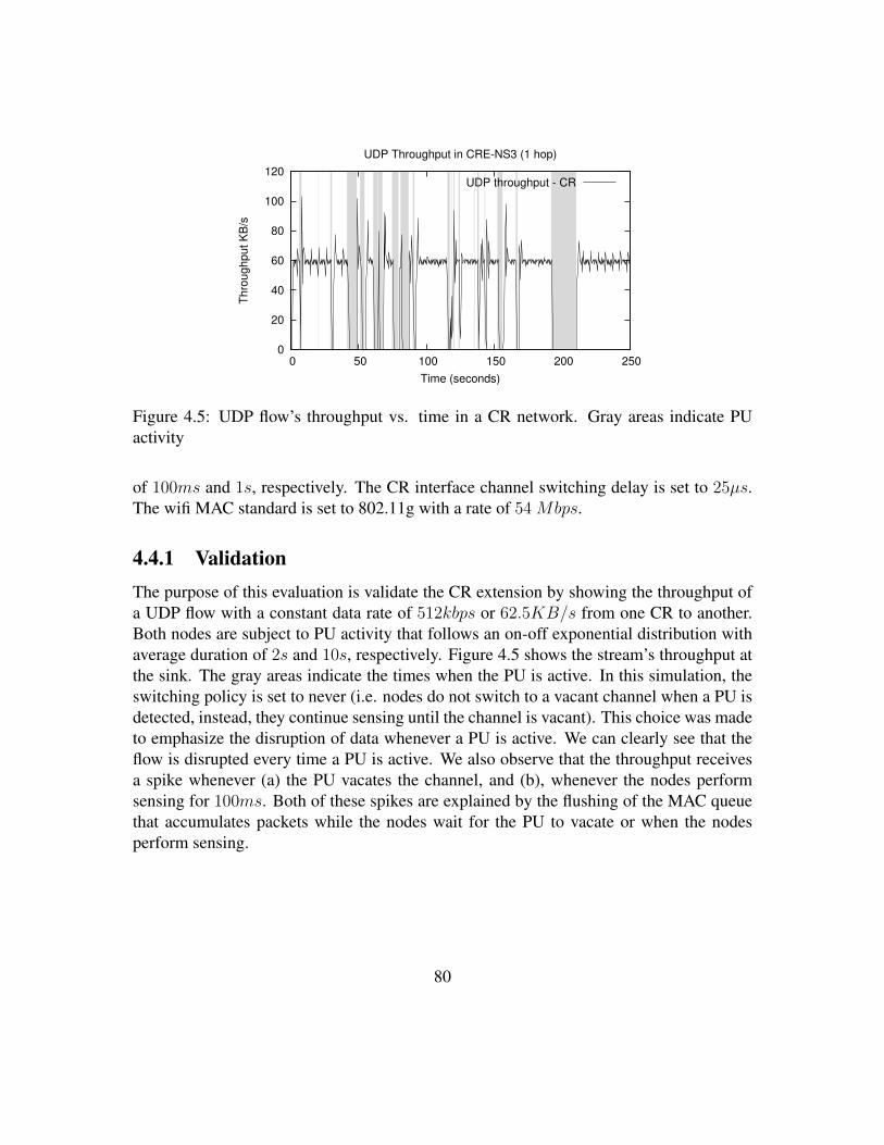
0

20

40

60

80

100

120

0 50 100 150 200 250

Th

rou

gh

pu

t K

B/s

Time (seconds)

UDP Throughput in CRE-NS3 (1 hop)

UDP throughput - CR

Figure 4.5: UDP flow’s throughput vs. time in a CR network. Gray areas indicate PUactivity

of 100ms and 1s, respectively. The CR interface channel switching delay is set to 25µs.The wifi MAC standard is set to 802.11g with a rate of 54 Mbps.

4.4.1 ValidationThe purpose of this evaluation is validate the CR extension by showing the throughput ofa UDP flow with a constant data rate of 512kbps or 62.5KB/s from one CR to another.Both nodes are subject to PU activity that follows an on-off exponential distribution withaverage duration of 2s and 10s, respectively. Figure 4.5 shows the stream’s throughput atthe sink. The gray areas indicate the times when the PU is active. In this simulation, theswitching policy is set to never (i.e. nodes do not switch to a vacant channel when a PU isdetected, instead, they continue sensing until the channel is vacant). This choice was madeto emphasize the disruption of data whenever a PU is active. We can clearly see that theflow is disrupted every time a PU is active. We also observe that the throughput receivesa spike whenever (a) the PU vacates the channel, and (b), whenever the nodes performsensing for 100ms. Both of these spikes are explained by the flushing of the MAC queuethat accumulates packets while the nodes wait for the PU to vacate or when the nodesperform sensing.

80

(a) (b)

Figure 4.6: Simulated CR network topologies (a) and (b)

4.4.2 CRE-NS3 overheadIn this evaluation, the nodes are placed in a topology as indicated by Figure 4.6(a). Eachnode sends constant rate data at 512 kbps to the immediate neighboring nodes as indicatedin the figure by the arrows for a total of 250 s. A set of 20 simulation runs are executed fora non-CR network, and then again for a CR network. The total execution time (kernel anduserspace in Linux’s time tool) and the maximum memory consumption using Valgrind’smassif tool [90] are then averaged over the 20 runs. Figure 4.7 shows the increase inboth CPU utilization and memory consumption by our proposed module. The memoryconsumption increases by about 0.8 MB and the CPU execution time increases by about10 s. The increase in both the execution and the memory consumption is mainly attributedto the fact that every CR node in the simulation has a combination of three total MAC-PHYinterfaces instead of one (See Figure 4.3).

4.4.3 CRE-NS3 vs. CRAHNDue to its similar architecture, in this section, CRAHN [85] in ns-2 is evaluated againstCRE-NS3 for the same network topology as depicted by Figure 4.6(b). The number ofnodes n increases with every simulation run until n = 13 or a total number of nodes of13 × 13 = 169. If i and j are a node’s row and column index, then each node sends astream to the nodes located at i + 1, j and i, j + 1 as depicted in the figure by the arrows.The stream that is sent from each node is a constant UDP flow with a bitrate of 512kbps.

81

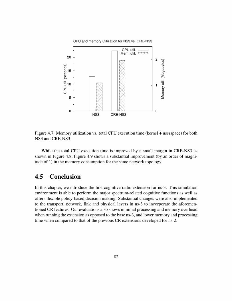
0

5

10

15

20

NS3 CRE-NS3 0

1

2

CP

U u

til. (

se

co

nd

s)

Me

mo

ry u

til. (

Me

ga

byte

s)

CPU and memory utilization for NS3 vs. CRE-NS3

CPU util.Mem. util.

Figure 4.7: Memory utilization vs. total CPU execution time (kernel + userspace) for bothNS3 and CRE-NS3

While the total CPU execution time is improved by a small margin in CRE-NS3 asshown in Figure 4.8, Figure 4.9 shows a substantial improvement (by an order of magni-tude of 1) in the memory consumption for the same network topology.

4.5 ConclusionIn this chapter, we introduce the first cognitive radio extension for ns-3. This simulationenvironment is able to perform the major spectrum-related cognitive functions as well asoffers flexible policy-based decision making. Substantial changes were also implementedto the transport, network, link and physical layers in ns-3 to incorporate the aforemen-tioned CR features. Our evaluations also shows minimal processing and memory overheadwhen running the extension as opposed to the base ns-3, and lower memory and processingtime when compared to that of the previous CR extensions developed for ns-2.

82

0

500

1000

1500

2000

2500

3000

0 2 4 6 8 10 12

Exe

cu

tio

n t

ime

(in

se

co

nd

s)

The square root of the number of nodes

CPU execution time

ns2ns3

Figure 4.8: Total CPU execution time (kernel + userspace) for both CRE-NS3 andCRAHN

1

10

100

1000

2 4 6 8 10 12

Me

mo

ry (

MB

)

Squareroot of the number of nodes

Memory (RAM) utilization

ns2ns3

Figure 4.9: Memory utilization (MB) for both CRE-NS3 and CRAHN

83

Conclusion

This thesis has covered considerable breadth in terms of the protocol stack layers that werestudied (e.g., transport, link and PHY), functionalities that were explored in these layers(e.g., rate control, interference alignment), as well as network architectural features (e.g.,spectrum databases, multi hop ad hoc networks, multi-transceiver nodes). Research on CRis necessarily cross-layered, and as this dissertation reveals, changes in any one aspect ofthe protocol stack has far reaching consequences on the ultimate end-to-end operation.

The thesis presents protocol design, experimentation, analysis, as well incorporatesdevising new simulation frameworks. We anticipate that the utility of this thesis will ex-tend beyond the included research results, allowing an active participation of students andresearchers in this exciting area through simulation studies made possible by our ns-3extension.

In summary, the thesis has focused on enhancing reliability, by both efficiently usingthe spectrum as well as identifying new spectrum that could be effectively used, withoutdegradation in the quality of service of licensed users. The main results are included below.

In Chapter 2, we presented an equation-based transport protocol, TFRC-CR, whichpresented a fundamentally different control mechanism compared to the typically usedTCP-based schemes. TFRC-CR was demonstrated to perform significantly better than itsclassical counterparts TFRC and TCP with respect to both PU protection and transmissionefficiency (in 2 hop scenarios, throughput for TFRC-CR is 100 KB/s while TFRC is 8KB/s and TCP is 12 KB/s). Our protocol does not assume any cross-layer feedback orinput from intermediate nodes, which aligns it with the traditional end-to-end paradigm inthe evolving space of transport layer research for multihop CR networks.

Chapter 3 describes a new paradigm for spectrum database access, which exploits thecorrelation that exists among two entirely different spectrum bands at specific locations,thereby improving the performance of local sensing. Results reveal about 23% reductionof queries, making it attractive for practical spectrum database deployments. In addition,we also explored a real-world interference alignment application that can reduce the con-trol channel utilization (5 time slots versus 35 for without IA). This non-trivial approachcan potentially open up a hitherto unexplored direction in spectrum sensing, and future

84

work will be focused on building the protocol suite that enables quick and efficient ex-change of spectrum data between the vehicles and the BSs.

Finally, in Chapter 4, we introduce the first cognitive radio extension for ns-3. Thissimulation environment is able to perform the major spectrum-related cognitive functionsas well as offers flexible policy-based decision making. Substantial changes were alsoimplemented to the transport, network, link and physical layers in ns-3 to incorporate theaforementioned CR features. Our evaluations also shows minimal processing and memoryoverhead (an increase of 0.8 MB only) when running the extension as opposed to the basens-3, and lower memory and processing time (memory is lower by an order of magnitudeof 1) when compared to that of the previous CR extensions developed for ns-2.

85

Publications

• A.K. Al-Ali, K.R. Chowdhury, ”TFRC-CR: An equation-based transport protocolfor cognitive radio networks”, in Proc. of IEEE ICNC, Washington, DC, USA,2013.

• A.K. Al-Ali, K.R. Chowdhury, ”TFRC-CR: An equation-based transport protocolfor cognitive radio networks”, Elsevier Ad Hoc Networks, vol. 11, no. 6, August2013.

• A.K. Al-Ali, K.R. Chowdhury, M. Di Felice and J. Paavola, ”Querying SpectrumDatabases and Improved Sensing for Vehicular Cognitive Radio Networks”, in Proc.of IEEE ICC, Sydney, Australia, Jun 2014.

• A.K. Al-Ali, Yifan Sun and K.R. Chowdhury, ”Accessing Spectrum Databases usingInterference Alignment in Vehicular Cognitive Radio Networks”, To appear in IEEETrans. on Vehic. Tech., Mar 2014.

86

Bibliography

[1] I. F. Akyildiz, W.-Y. Lee, and K. R. Chowdhury, “CRAHNs: cognitive radio ad hocnetworks,” Ad Hoc Netw., vol. 7, no. 5, pp. 810–836, Jul. 2009. [Online]. Available:http://dx.doi.org/10.1016/j.adhoc.2009.01.001

[2] Cisco systems, Inc., “Cisco visual networking index: Global mobiledata traffic forecast update, 20122017,” February 2013. [Online]. Avail-able: http://www.cisco.com/en/US/solutions/collateral/ns341/ns525/ns537/ns705/ns827/white paper c11-520862.html

[3] Ericsson, Inc., “Ericsson mobility report,” June 2013. [Online]. Available:http://www.ericsson.com/res/docs/2013/ericsson-mobility-report-june-2013.pdf

[4] “FCC, spectrum policy task force report,” ET Docket No. 02-135, November 2002.

[5] P. K. et al., “Next generation communications: Kickoff meeting,” in Proc. DARPA,October 2001.

[6] M. McHenry, “Frequency agile spectrum access technologies,” in FCC WorkshopCogn. Radio, May 2003.

[7] G. Staple and K. Werbach, “The end of spectrum scarcity [spectrum allocation andutilization],” Spectrum, IEEE, vol. 41, no. 3, pp. 48–52, 2004.

[8] J. Mitola and J. Maguire, G.Q., “Cognitive radio: making software radios more per-sonal,” Personal Communications, IEEE, vol. 6, no. 4, pp. 13–18, 1999.

[9] S. Haykin, “Cognitive radio: brain-empowered wireless communications,” SelectedAreas in Communications, IEEE Journal on, vol. 23, no. 2, pp. 201–220, 2005.

[10] K. Chowdhury, M. Di Felice, and I. Akyildiz, “TP-CRAHN: a transport protocol forcognitive radio ad-hoc networks,” in INFOCOM 2009, IEEE, 2009, pp. 2482–2490.

87

[11] K. Sundaresan, V. Anantharaman, H.-Y. Hsieh, and R. Sivakumar, “ATP: a reliabletransport protocol for ad hoc networks,” Mobile Computing, IEEE Transactions on,vol. 4, no. 6, pp. 588–603, 2005.

[12] “FCC, establishment of interference temperature metric to quantify and manage in-terference and to expand available unlicensed operation in certain xed mobile andsatellite frequency bands,” ET Docket No. 03-237, DA 03-289, November 2003.

[13] T. Clancy, “Dynamic spectrum access using the interference temperature model,”annals of telecommunications - annales des tlcommunications, vol. 64, no. 7-8, pp.573–592, 2009. [Online]. Available: http://dx.doi.org/10.1007/s12243-009-0098-x

[14] Y. Xing, C. Mathur, M. Haleem, R. Chandramouli, and K. P. Subbalakshmi, “Dy-namic spectrum access with qos and interference temperature constraints,” MobileComputing, IEEE Transactions on, vol. 6, no. 4, pp. 423–433, 2007.

[15] M. Sharma, A. Sahoo, and K. D. Nayak, “Channel selection under interference tem-perature model in multi-hop cognitive mesh networks,” in New Frontiers in DynamicSpectrum Access Networks, 2007. DySPAN 2007. 2nd IEEE International Sympo-sium on, 2007, pp. 133–136.

[16] J. Bater, H. Tan, K. Brown, and L. Doyle, “Modelling interference temperature con-straints for spectrum access in cognitive radio networks,” in Communications, 2007.ICC ’07. IEEE International Conference on, 2007, pp. 6493–6498.

[17] “FCC, establishment of interference temperature metric to quantify and manage in-terference and to expand available unlicensed operation in certain xed mobile andsatellite frequency bands,” ET Docket No. 03-237, DA 07-78, May 2007.

[18] “FCC, facilitating opportunities for flexible, efficient, and reliable spectrum use em-ploying cognitive radio technologies,” ET Docket No. 03-322, DA 03-108, December2003.

[19] Q. Zhao, L. Tong, and A. Swami, “Decentralized cognitive mac for dynamic spec-trum access,” in New Frontiers in Dynamic Spectrum Access Networks, 2005. DyS-PAN 2005. 2005 First IEEE International Symposium on, 2005, pp. 224–232.

[20] S. Sankaranarayanan, P. Papadimitratos, A. Mishra, and S. Hershey, “A bandwidthsharing approach to improve licensed spectrum utilization,” in New Frontiers in Dy-namic Spectrum Access Networks, 2005. DySPAN 2005. 2005 First IEEE Interna-tional Symposium on, 2005, pp. 279–288.

88

[21] H. Zheng and C. Peng, “Collaboration and fairness in opportunistic spectrum access,”in Communications, 2005. ICC 2005. 2005 IEEE International Conference on, vol. 5,2005, pp. 3132–3136 Vol. 5.

[22] W. Wang and X. Liu, “List-coloring based channel allocation for open-spectrumwireless networks,” in Vehicular Technology Conference, 2005. VTC-2005-Fall. 2005IEEE 62nd, vol. 1, 2005, pp. 690–694.

[23] M. Steenstrup, “Opportunistic use of radio-frequency spectrum: a network perspec-tive,” in New Frontiers in Dynamic Spectrum Access Networks, 2005. DySPAN 2005.2005 First IEEE International Symposium on, 2005, pp. 638–641.

[24] C. Peng, H. Zheng, and B. Zhao, “Utilization and fairness in spectrumassignment for opportunistic spectrum access,” Mobile Networks and Applications,vol. 11, no. 4, pp. 555–576, 2006. [Online]. Available: http://dx.doi.org/10.1007/s11036-006-7322-y

[25] L. Cao and H. Zheng, “Understanding the power of distributed coordination fordynamic spectrum management,” Mobile Networks and Applications, vol. 13,no. 5, pp. 477–497, 2008. [Online]. Available: http://dx.doi.org/10.1007/s11036-008-0086-9

[26] Y. Chen, Q. Zhao, and A. Swami, “Joint design and separation principle for oppor-tunistic spectrum access,” in Proc. IEEE Asilomar Conference on Signals, Systemsand Computers 2006, October 2006.

[27] “FCC, unlicensed operation in the tv broadcast bands, and additional spectrum forunlicensed devices below 900 mhz and in the 3 ghz band,” ET Docket No. 10-174,DA 04-186, September 2010.

[28] “FCC, second memorandum opinion and order,” ET Docket No. 04-186, DA 11-131,January 2011.

[29] “Office of engineering and technology seeks comment on microsoft corporation pro-posal to be designated as a tv bands device database administrator,” ET Docket No.04-186, DA 11-803, April 2011.

[30] “FCC, order,” ET Docket No. 04-186, DA 11-1291, July 2011.

[31] FCC, “Database administrators for unlicensed wireless micro-phones,” October 2013. [Online]. Available: http://www.fcc.gov/help/database-administrators-unlicensed-wireless-microphones

89

[32] Key Bridge Global LLC, “Key bridge white space portal,” October 2013. [Online].Available: https://keybridgeglobal.com/whitespace/

[33] Google, Inc., “Google spectrum database,” October 2013. [Online]. Available:http://www.google.org/spectrum/whitespace/

[34] “Spectrum bridge.” [Online]. Available: http://www.spectrumbridge.com/

[35] Frequency Finder, Inc., “Radiosoft - radio propagation software and fcc form 601software & filing,” October 2013. [Online]. Available: http://radiosoft.com/

[36] KB Enterprises, Inc., “LS Telcom,” October 2013. [Online]. Available: http://www.lstelcom.com/

[37] NeuStar, Inc., “Neustar — real intelligence, better decisions,” October 2013.[Online]. Available: http://www.neustar.biz/

[38] Telcordia Technologies, Inc., October 2013. [Online]. Available: http://www.telcordia.com/

[39] Airity, Inc. (formerly WSdb LLC), October 2013. [Online]. Available: http://www.2M.com/

[40] Microsoft, Inc., “Microsoft research white space finder,” October 2013. [Online].Available: http://whitespaces.cloudapp.net/

[41] Comsearch, October 2013. [Online]. Available: http://www.comsearch.com/

[42] V. Cadambe and S. Jafar, “Interference alignment and degrees of freedom of the k -user interference channel,” Information Theory, IEEE Transactions on, vol. 54, no. 8,pp. 3425–3441, 2008.

[43] X. Chang, “Network simulations with opnet,” in Proceedings of the 31st conferenceon Winter simulation: Simulation—a bridge to the future-Volume 1. ACM, 1999,pp. 307–314.

[44] T. R. Henderson, M. Lacage, and G. F. Riley, “Network Simulations with the ns-3Simulator,” in ACM SIGCOMM’08. ACM, Aug. 2008, p. 527.

[45] “Doxygen.” [Online]. Available: http://www.stack.nl/∼dimitri/doxygen/

[46] D. Sarkar and H. Narayan, “Transport layer protocols for cognitive networks,” in IN-FOCOM IEEE Conference on Computer Communications Workshops , 2010, 2010,pp. 1–6.

90

[47] X. Wang, X. Sun, C. Zhao, and Z. Zhou, “TCP-CReno – tcp enhancement usingcross-layer for cognitive radio networks,” in Advanced Intelligence and AwarenssInternet (AIAI 2010), 2010 International Conference on, 2010, pp. 37–40.

[48] S. Floyd, M. Handley, J. Padhye, and J. Widmer, “Equation-based congestion controlfor unicast applications,” SIGCOMM Comput. Commun. Rev., vol. 30, no. 4, pp.43–56, Aug. 2000. [Online]. Available: http://doi.acm.org/10.1145/347057.347397

[49] T. Goff, J. Moronski, D. Phatak, and V. Gupta, “Freeze-tcp: a true end-to-end tcpenhancement mechanism for mobile environments,” in INFOCOM 2000. NineteenthAnnual Joint Conference of the IEEE Computer and Communications Societies. Pro-ceedings. IEEE, vol. 3, 2000, pp. 1537–1545 vol.3.

[50] P. Sinha, T. Nandagopal, N. Venkitaraman, R. Sivakumar, and V. Bharghavan,“Wtcp: a reliable transport protocol for wireless wide-area networks,” Wirel.Netw., vol. 8, no. 2/3, pp. 301–316, Mar. 2002. [Online]. Available: http://dx.doi.org/10.1023/A:1013702428498

[51] G. Holland and N. Vaidya, “Analysis of tcp performance over mobile ad hocnetworks,” in Proceedings of the 5th annual ACM/IEEE international conference onMobile computing and networking, ser. MobiCom ’99. New York, NY, USA: ACM,1999, pp. 219–230. [Online]. Available: http://doi.acm.org/10.1145/313451.313540

[52] M. Mathis, J. Mahdavi, S. Floyd, and A. Romanow, “RFC 2018: TCP SelectiveAcknowledgment Options,” in Internet Society Conference, 1996.

[53] M. D. Felice, K. R. Chowdhury, W. Kim, A. Kassler, and L. Bononi, “End-to-end protocols for cognitive radio ad hoc networks: An evaluation study,”Performance Evaluation, vol. 68, no. 9, pp. 859 – 875, 2011, ¡ce:title¿SpecialIssue: Advances in Wireless and Mobile Networks¡/ce:title¿. [Online]. Available:http://www.sciencedirect.com/science/article/pii/S0166531610001604

[54] A. O. Bicen and O. B. Akan, “Reliability and congestion control in cognitive radiosensor networks,” Ad Hoc Networks, vol. 9, no. 7, pp. 1154 – 1164, 2011. [Online].Available: http://www.sciencedirect.com/science/article/pii/S1570870511000163

[55] H. Xiao, K. C. Chua, J. Malcolm, and Y. Zhang, “Theoretical analysis of tcp through-put in adhoc wireless networks,” in Global Telecommunications Conference, 2005.GLOBECOM ’05. IEEE, vol. 5, 2005, pp. 6 pp.–2719.

91

[56] A. Slingerland, P. Pawelczak, R. Venkatesha Prasad, A. Lo, and R. Hekmat, “Per-formance of transport control protocol over dynamic spectrum access links,” in NewFrontiers in Dynamic Spectrum Access Networks, 2007. DySPAN 2007. 2nd IEEEInternational Symposium on, 2007, pp. 486–495.

[57] C. Luo, F. R. Yu, H. Ji, and V. C. Leung, “Optimal channel access for tcp performanceimprovement in cognitive radio networks,” Wirel. Netw., vol. 17, no. 2, pp. 479–492,Feb. 2011. [Online]. Available: http://dx.doi.org/10.1007/s11276-010-0292-9

[58] C. Luo, F. Yu, H. Ji, and V. Leung, “Cross-layer design for tcp performance im-provement in cognitive radio networks,” Vehicular Technology, IEEE Transactionson, vol. 59, no. 5, pp. 2485–2495, 2010.

[59] A. Kumar and K. Shin, “Managing tcp connections in dynamic spectrum accessbased wireless lans,” in Sensor Mesh and Ad Hoc Communications and Networks(SECON), 2010 7th Annual IEEE Communications Society Conference on, 2010, pp.1–9.

[60] M. Faisal Amjad, B. Aslam, and C. Zou, “Transparent cross-layer solutions forthroughput boost in cognitive radio networks,” in Consumer Communications andNetworking Conference (CCNC), 2013 IEEE, 2013, pp. 580–586.

[61] N. Bapat and V. Syrotiuk, “Adapting sensing and transmission times to improvethroughput in cognitive radios ad hoc networks,” in World of Wireless, Mobile andMultimedia Networks (WoWMoM), 2012 IEEE International Symposium on a, 2012,pp. 1–6.

[62] Y. Ko and N. Vaidya, “Locationaided routing (lar) in mobile ad hoc networks,”Wireless Networks, vol. 6, no. 4, pp. 307–321, 2000. [Online]. Available:http://dx.doi.org/10.1023/A%3A1019106118419

[63] V. Jacobson, “Congestion avoidance and control,” SIGCOMM Comput. Commun.Rev., vol. 18, no. 4, pp. 314–329, Aug. 1988. [Online]. Available: http://doi.acm.org/10.1145/52325.52356

[64] GitHub, Inc., “abdulla al-ali/tfrc-cr.” [Online]. Available: https://github.com/abdulla-alali/TFRC-CR/tree/CRAHN/

[65] W.-Y. Lee and I. Akyildiz, “Optimal spectrum sensing framework for cognitive ra-dio networks,” Wireless Communications, IEEE Transactions on, vol. 7, no. 10, pp.3845–3857, 2008.

92

[66] M. Di Felice, R. Doost-Mohammady, K. R. Chowdhury, and L. Bononi, “Smart ra-dios for smart vehicles: Cognitive vehicular ad hoc networks,” IEEE Vehicular Tech-nology Magazine, vol. 7, no. 2, 2012.

[67] K. Miller, A. Sanne, K. Srinivasan, and S. Vishwanath, “Enabling real-time interfer-ence alignment: Promises and challenges,” in Proc. of ACM MobiHoc ’12. ACM,2012, pp. 55–64.

[68] K. Fawaz, A. Ghandour, M. Olleik, and H. Artail, “Improving reliability of safetyapplications in vehicle ad hoc networks through the implementation of a cognitivenetwork,” in Proc. IEEE ICT, 2010, pp. 798–805.

[69] H. Li and D. Irick, “Collaborative spectrum sensing in cognitive radio vehicular adhoc networks: Belief propagation on highway,” in Proc. of IEEE VTC Spring, 2010,pp. 1–5.

[70] X. Y. Wang and P.-H. Ho, “A novel sensing coordination framework for cr-vanets,”Vehicular Technology, IEEE Transactions on, vol. 59, no. 4, pp. 1936–1948, 2010.

[71] M. Di Felice, K. Chowdhury, and L. Bononi, “Analyzing the potential of cooperativecognitive radio technology on inter-vehicle communication,” in Wireless Days (WD),2010 IFIP, 2010, pp. 1–6.

[72] S. Pagadarai, A. M. Wyglinski, and R. Vuyyuru, “Characterization of vacant uhf tvchannels for vehicular dynamic spectrum access,” in Vehicular Networking Confer-ence (VNC), 2009 IEEE, 2009, pp. 1–8.

[73] T. Gou, C. Wang, and S. A. Jafar, “Aiming perfectly in the dark - blind interferencealignment through staggered antenna switching.” in GLOBECOM. IEEE, 2010, pp.1–5.

[74] S. Gollakota, S. D. Perli, and D. Katabi, “Interference alignment and cancellation,”SIGCOMM Comput. Commun. Rev., vol. 39, no. 4, pp. 159–170, Aug. 2009.

[75] J. I. Choi, M. Jain, K. Srinivasan, P. Levis, and S. Katti, “Achieving single channel,full duplex wireless communication,” in Proc. of ACM MobiCom ’10. New York,NY, USA: ACM, 2010, pp. 1–12.

[76] M. Jain, J. I. Choi, T. Kim, D. Bharadia, S. Seth, K. Srinivasan, P. Levis, S. Katti,and P. Sinha, “Practical, real-time, full duplex wireless,” in Proc. of ACM MobiCom’11. New York, NY, USA: ACM, 2011, pp. 301–312.

93

[77] “Ettus research.” [Online]. Available: http://www.ettus.com/

[78] W.-Y. Lee and I. Akyildiz, “Optimal spectrum sensing framework for cognitive ra-dio networks,” Wireless Communications, IEEE Transactions on, vol. 7, no. 10, pp.3845–3857, 2008.

[79] H. Urkowitz, “Energy detection of unknown deterministic signals,” Proceedings ofthe IEEE, vol. 55, no. 4, pp. 523–531, 1967.

[80] A. Sonnenschein and P. Fishman, “Radiometric detection of spread-spectrum signalsin noise of uncertain power,” Aerospace and Electronic Systems, IEEE Transactionson, vol. 28, no. 3, pp. 654–660, 1992.

[81] “Cognitive Radio Cognitive Network Simulator,” [accessed 03-Feb-2014]. [Online].Available: http://faculty.uml.edu/Tricia Chigan/Research/CRCN Simulator.htm

[82] V. Esmaeelzadeh, R. Berangi, S. Sebt, E. Hosseini, and M. Parsinia, “Cogns: A simu-lation framework for cognitive radio networks,” Wireless Personal Communications,vol. 72, no. 4, 2013.

[83] J. Marinho and E. Monteiro, “Cognitive radio simulation based on omnet++/mixim,”in Proc. of the 11th Conferencia sobre Redes de Computadores, 2011.

[84] M. Zhan, P. Ren, and M. Gong, “An open software simulation platform for cognitiveradio,” in Wireless Communications Networking and Mobile Computing (WiCOM),2010 6th International Conference on, Sept 2010, pp. 1–4.

[85] M. D. Felice, K. R. Chowdhury, W. Kim, A. Kassler, and L. Bononi, “End-to-endprotocols for cognitive radio ad hoc networks: An evaluation study,” PerformanceEvaluation, vol. 68, no. 9, pp. 859 – 875, 2011.

[86] “OMNeT++ Network Simulation Framework,” [accessed 03-Feb-2014]. [Online].Available: http://www.omnetpp.org/

[87] A. K. Al-Ali and K. Chowdhury, “TFRC-CR: An equation-based transport protocolfor cognitive radio networks,” Ad Hoc Networks, vol. 11, no. 6, 2013.

[88] C. Perkins and E. Royer, “Ad-hoc on-demand distance vector routing,” in MobileComputing Systems and Applications, 1999. Proceedings. WMCSA ’99. Second IEEEWorkshop on, Feb 1999, pp. 90–100.

[89] D. C. Plummer, “An Ethernet address resolution protocol - RFC 826,” Nov 1982.

94

[90] N. Nethercote and J. Seward, “Valgrind: A framework for heavyweight dynamicbinary instrumentation,” ACM SIGPLAN Not., vol. 42, no. 6, Jun. 2007.

95