Data Warehousing and Decision Support

CS634Class 22, Apr 25, 2016

Slides based on “Database Management Systems” 3rd ed, Ramakrishnan and Gehrke, Chapter 25

Introduction

Increasingly, organizations are analyzing current and historical data to identify useful patterns and support business strategies.

Emphasis is on complex, interactive, exploratory analysis of very large datasets created by integrating data from across all parts of an enterprise; data is fairly static.• Contrast such Data Warehousing and On-Line Analytic Processing

(OLAP) with traditional On-line Transaction Processing (OLTP):mostly long queries, instead of the short update Xacts of OLTP.

• These are both using “structured data” that can be fairly easily loaded into a database

Structured vs. Unstructured Data

• So far, we have been working with structured data

• Structured data:• Entities with attributes, each fitting a SQL data type

• Relationships

• Each row of data is precious

• Loads into relational tables, long-term storage

• Can be huge

• Unstructured data, realm of “big data”• Often doesn’t fit into E/R model, too sloppy

• Each piece of data is not precious—it’s statistical

• Sometimes just processed and thrown away

• No permanent specialized repository, maybe saved in files

• Can be really huge

Bigness of Data

Big data warehouses, all on Teradata systems

See http://gigaom.com/2013/03/27/why-apple-ebay-and-walmart-have-some-of-the-biggest-data-warehouses-youve-ever-seen• Biggest DW: Walmart, passed 1TB in 1992, 2.8 PB (petabytes) = 2800 TB in

2008, 30 PB in 2014, growing…

• eBay: 9 PB DW in 2013, also has 40 PB of big data

• Apple: multiple-PB DW

• Big data:• Usually over 50TB, can’t fit on one machine

• Is judged by “velocity” as well as size

• Google: processed 24 PB of data per day in 2009, invented Map-Reduce, published 2004

Teradata

• Teradata provides a relational database with ANSI compliant SQL, targeted to data warehouses

• Proprietary, expensive ($millions)

• Uses a shared-nothing architecture on many independent nodes

• Partitioning by rows or (more recently) columns

• Scales up well: add node, add network bandwidth for it

Three Complementary Trends

Data Warehousing: Consolidate data from many sources in one large repository (relational database).• Loading, periodic synchronization of replicas.

• Semantic integration, Data cleaning of data on way in

• Both simple and complex SQL queries and views.

OLAP:• Complex SQL queries (in effect, but not composed by users).

• Queries based on spreadsheet-style operations and “multidimensional”view of data.

• Interactive and “online” queries.

Data Mining: Exploratory search for interesting trends and anomalies.

Data Warehousing

Integrated data spanning long time periods, often augmented with summary information.

Several gigabytes to terabytes common, now petabytes too.

Interactive response times expected for complex queries; ad-hoc updates uncommon.

Read-mostly data

EXTERNAL DATA SOURCES

EXTRACT

TRANSFORM

LOAD

REFRESH

DATA

WAREHOUSEMetadata

Repository

SUPPORTS

OLAPDATA

MINING

Warehousing Issues

Semantic Integration: When getting data from multiple sources, must eliminate mismatches, e.g., different currencies, schemas.

Heterogeneous Sources: Must access data from a variety of source formats and repositories.• Replication capabilities can be exploited here.

Load, Refresh, Purge: Must load data, periodically refresh it, and purge too-old data.

Metadata Management: Must keep track of source (lineage) loading time, and other information for all data in the warehouse.

OLAP: Multidimensional data model

• Example: sales data

• Dimensions: Product, Location, Time

• A measure is a numeric value like sales we want to understand in terms of the dimensions

• Example measure: dollar sales value “sales”

• Example data point (one row of fact/cube table):• Sales = 25 for pid=1, timeid=1, locid=1 is the sum of sales for that day, in that location, for

that product

• Pid=1: details in Product table

• Locid = 1: details in Location table

•Note aggregation here: sum of sales is most detailed data

Multidimensional Data Model

Collection of numeric measures, which depend on a set of dimensions. E.g., measure sales, dimensions Product (key: pid), Location

(locid), and Time (timeid).

Full table, pg. 851

8 10 10

30 20 50

25 8 15

1 2 3

timeid

pid

11 12 1

3

11 1 1 25

11 2 1 8

11 3 1 15

12 1 1 30

12 2 1 20

12 3 1 50

13 1 1 8

13 2 1 10

13 3 1 10

11 1 2 35

pid

tim

eid

loci

d

sale

s

locid

Slice locid=1

is shown:

SalesCube(pid, timeid, locid, sales)

Granularity of Data

• Example of last slide uses time at granularity of days

• Individual transactions (sales at cashier) have been added together to make one row in this table

• Note: “measures” can always be aggregated

• Current hardware can handle more data

• Typical data warehouses hold the original transaction data

• So such a fact table has more columns, for example

• dateid, timeofday, prodid, storeid, txnid, clerkid, sales, …

Data Warehouse vs. Data for OLAP

• Current DW fact table is huge, with individual transactions, large number of dimensions

• Can only use a subset of this for OLAP, because of explosion of cells

• Take DW fact table, roll up to days (say), drop less important columns, get much smaller data for OLAP

• Load data into OLAP, another tool.

• Table on pg. 851 is a cube table, not a DW fact table

• Can think of OLAP as a cache of most important aggregates of DW tables

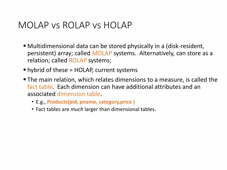
MOLAP vs ROLAP vs HOLAP

Multidimensional data can be stored physically in a (disk-resident, persistent) array; called MOLAP systems. Alternatively, can store as a relation; called ROLAP systems;

hybrid of these = HOLAP, current systems

The main relation, which relates dimensions to a measure, is called the fact table. Each dimension can have additional attributes and an associated dimension table.• E.g., Products(pid, pname, category,price )

• Fact tables are much larger than dimensional tables.

Dimension Hierarchies: OLAP, DW

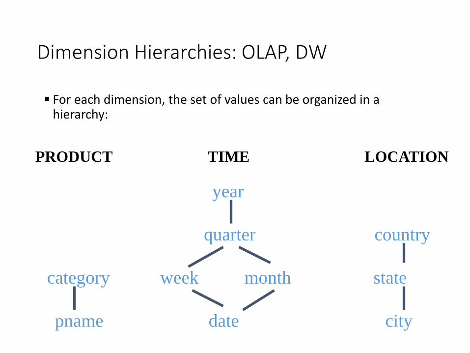
For each dimension, the set of values can be organized in a hierarchy:

PRODUCT TIME LOCATION

category week month state

pname date city

year

quarter country

Schema underlying OLAP, used in DW

Fact/cube table in BCNF; dimension tables not normalized.• Dimension tables are small; updates/inserts/deletes are rare. So, anomalies

less important than good query performance.

This kind of schema is very common in DW and OLAP, and is called a star schema; computing the join of all these relations is called a star join.Note: in OLAP, this is not what the user sees, it’s hidden underneath In DW, this is the basic setup, but usually with more dimensionsHere only one measure, sales, but can have several

pricecategorypnamepid countrystatecitylocid

saleslocidtimeidpid

holiday_flagweekdatetimeid month quarter year

(Fact table)SALES

TIMES

PRODUCTS LOCATIONS

OLAP (and DW) Queries

Influenced by SQL and by spreadsheets.

A common operation is to aggregate a measure over one or more dimensions.• Find total sales.

• Find total sales for each city, or for each state.

• Find top five products ranked by total sales.

Roll-up: Aggregating at different levels of a dimension hierarchy. • E.g., Given total sales by city, we can roll-up to get sales by state.

OLAP Queries: MDX (Multidimensional Expressions)

• Originally a Microsoft SQL Server project, but now supported widely in the OLAP industry: Oracle, SAS, SAP, Teradata on server side, as well as Microsoft. Allows client programs to specify OLAP datasets.

• Example from Wikipedia

SELECT

{ [Measures].[Store Sales] } ON COLUMNS,

{ [Date].[2002], [Date].[2003] } ON ROWS

FROM Sales

WHERE ( [Store].[USA].[CA] )

• The SELECT clause sets the query axes as the Store Sales member of the Measures dimension, and the 2002 and 2003 members of the Date dimension.

• The FROM clause indicates that the data source is the Sales cube.• The WHERE clause defines the "slicer axis" as the California member of

the Store dimension.

OLAP Queries

Drill-down: The inverse of roll-up: go from sum to details that were added up before• E.g., Given total sales by state, can drill-down to get total sales by county.

• Drill down again, see total sales by city

• E.g., Can also drill-down on different dimension to get total sales by product for each state.

OLAP Queries: cross-tabs

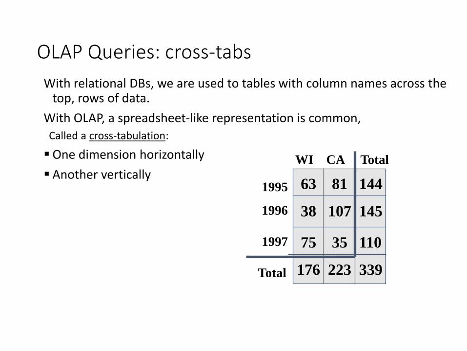
With relational DBs, we are used to tables with column names across the top, rows of data.

With OLAP, a spreadsheet-like representation is common,

Called a cross-tabulation:

One dimension horizontally

Another vertically63 81 144

38 107 145

75 35 110

WI CA Total

1995

1996

1997

176 223 339Total

OLAP Queries: Pivoting Example cross-tabulation:

Pivoting: switching dimensions on axes, or choosing what dimensions to show on axes

Switching dimensions means pivoting around a point in the upper-left-hand corner End up with “1995 1996 1997 Total” across top, “WI CA Total” down the side

63 81 144

38 107 145

75 35 110

WI CA Total

1995

1996

1997

176 223 339Total

Oracle 11 supports cross-tabs display

select * from (

select times_purchased, state_code

from customers t

) pivot (

count(state_code)

for state_code in ('NY','CT','NJ','FL','MO')

) order by times_purchased

Here is the output:

TIMES_PURCHASED 'NY' 'CT‘ 'NJ' 'FL‘ 'MO'

--------------- ---------- ---------- ---------- ---------- --

0 16601 90 0 0 0

1 33048 165 0 0 0

2 33151 179 0 0 0

3 32978 173 0 0 0

4 33109 173 0 1 0

... and so on ... (We have Oracle 10, unfortunately)

SQL Queries for cross-tab entries

The cross-tabulation values can be computed using a collection of SQL queries:

SELECT SUM(S.sales)

FROM Sales S, Times T, Locations L

WHERE S.timeid=T.timeid AND S.timeid=L.timeid

GROUP BY T.year, L.state

SELECT SUM(S.sales)

FROM Sales S, Times T

WHERE S.timeid=T.timeid

GROUP BY T.year

SELECT SUM(S.sales)

FROM Sales S, Location L

WHERE S.timeid=L.timeid

GROUP BY L.state

63 81 144

38 107 145

75 35 110

WI CA Total

1995

1996

1997

176 223 339Total

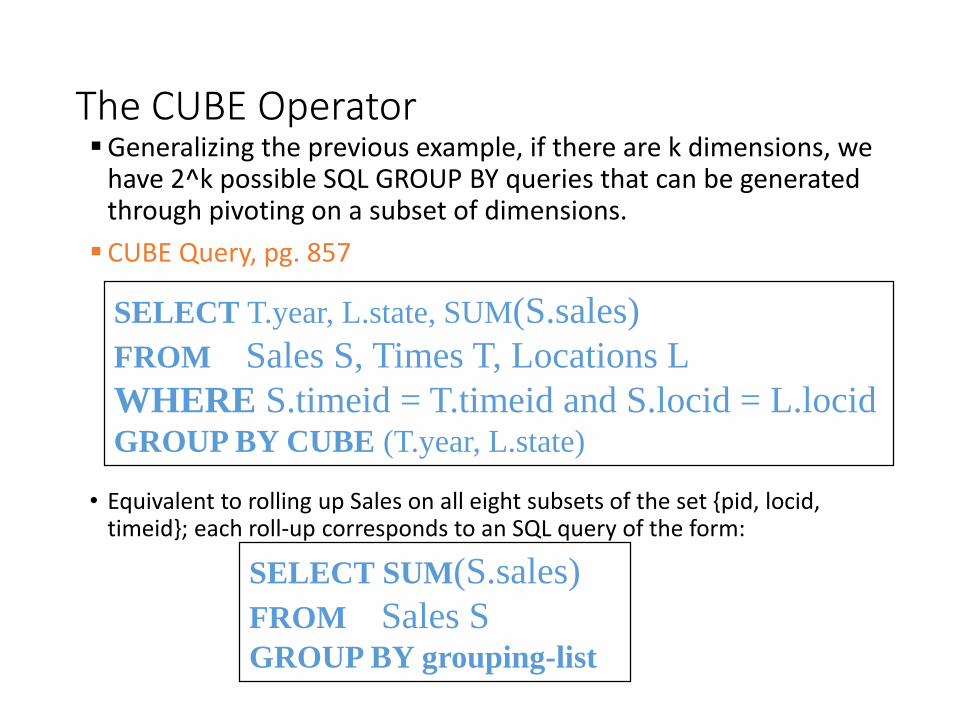
The CUBE OperatorGeneralizing the previous example, if there are k dimensions, we

have 2^k possible SQL GROUP BY queries that can be generated through pivoting on a subset of dimensions.

CUBE Query, pg. 857

• Equivalent to rolling up Sales on all eight subsets of the set {pid, locid, timeid}; each roll-up corresponds to an SQL query of the form:

SELECT SUM(S.sales)

FROM Sales SGROUP BY grouping-list

SELECT T.year, L.state, SUM(S.sales)

FROM Sales S, Times T, Locations L

WHERE S.timeid = T.timeid and S.locid = L.locidGROUP BY CUBE (T.year, L.state)

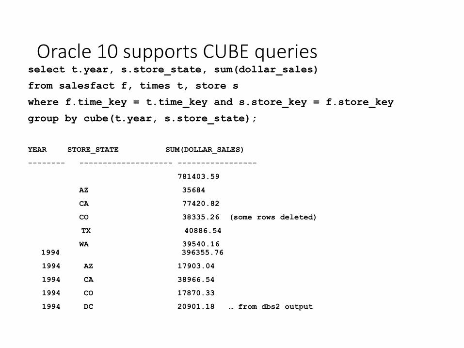
Oracle 10 supports CUBE queriesselect t.year, s.store_state, sum(dollar_sales)

from salesfact f, times t, store s

where f.time_key = t.time_key and s.store_key = f.store_key

group by cube(t.year, s.store_state);

YEAR STORE_STATE SUM(DOLLAR_SALES)

-------- -------------------- -----------------

781403.59

AZ 35684

CA 77420.82

CO 38335.26 (some rows deleted)

TX 40886.54

WA 39540.16

1994 396355.76

1994 AZ 17903.04

1994 CA 38966.54

1994 CO 17870.33

1994 DC 20901.18 … from dbs2 output

DW data OLAP

• The CUBE query can do the roll-ups on DW data needed for OLAP

Excel is the champ at OLAP queries

• Next time will do Excel pivot table demo

• Based on video by Minder Chen of UCI (Cal state U/Channel Islands)

• https://www.youtube.com/watch?v=eGhjklYyv6Y

• Setup:

• His MS Access database with star schema for sales

• Create view of fact joined with desired dimension data (a star join)

• Point Excel at this big view, ask it to create pivot table

• Pivot table: drill down, roll up, pivot, …

Excel can use Oracle data too

• The database from Chen’s demo is now in dbs2’s Oracle

• We could point Excel to an Oracle view of joined tables.

• How does that work?

• Use ODBC (Open Database Connectivity), older than JDBC, but roughly same idea• Provides client API for accessing multiple databases

• Each database provides a ODBC driver

• Unfortunately, it’s not easy to set up ODBC on a Windows system even though Microsoft invented it

• Another way: MDX driver to allow Excel to use live Oracle OLAP data

• http://download.oracle.com/otndocs/products/warehouse/olap/videos/excel_olap_demo/Excel_Demo_for_Web.html

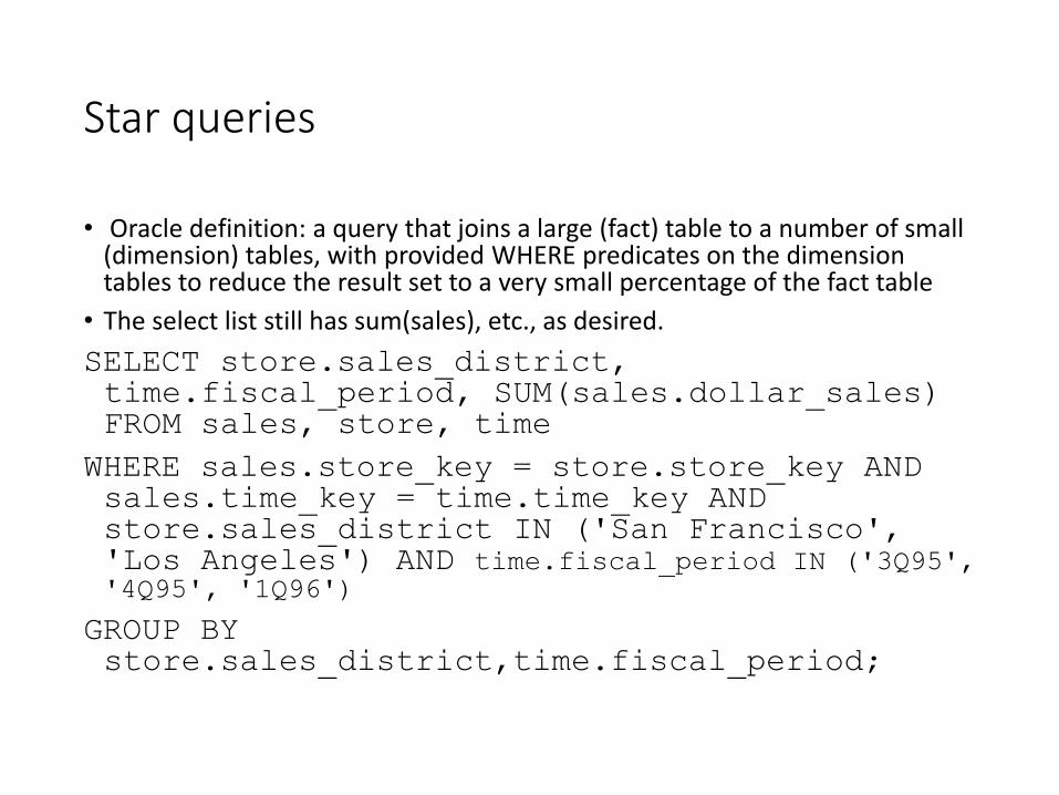
Star queries

• Oracle definition: a query that joins a large (fact) table to a number of small (dimension) tables, with provided WHERE predicates on the dimension tables to reduce the result set to a very small percentage of the fact table

• The select list still has sum(sales), etc., as desired.

SELECT store.sales_district, time.fiscal_period, SUM(sales.dollar_sales) FROM sales, store, time

WHERE sales.store_key = store.store_key AND sales.time_key = time.time_key AND store.sales_district IN ('San Francisco', 'Los Angeles') AND time.fiscal_period IN ('3Q95', '4Q95', '1Q96')

GROUP BY store.sales_district,time.fiscal_period;

Star queries

• Oracle: A better way to write the query would be:(i.e., give the QP a hint on how to do it)

SELECT ... FROM sales WHERE store_key IN ( SELECT store_key FROM store

WHERE sales_district IN ('WEST', 'SOUTHWEST')) AND time_key IN

( SELECT time_key FROM time WHERE quarter IN ('3Q96', '4Q96', '1Q97'))

AND product_key IN( SELECT product_key FROM product

WHERE department = 'GROCERY')GROUP BY …;

• Oracle will rewrite the query this way if you add the STAR_TRANSFORMATION hint to your SQL, or the DBA has set STAR_TRANSFORMATION_ENABLED

Excel can do Star queries

• Recall GROUP BY queries for individual crosstab entries

• A Star query is of this form, plus WHERE clause predicates on dimension tables such as• store.sales_district IN ('WEST', 'SOUTHWEST')

• time.quarter IN ('3Q96', '4Q96', '1Q97')

• Excel allows “filters” on data that correspond to these predicates of the WHERE clause

Indexes related to data warehousing

New indexing techniques: Bitmap indexes, Join indexes, array representations, compression, precomputation of aggregations, etc.

E.g., Bitmap index:

sex custid name sex rating ratingBit-vector:

1 bit for each

possible value.

Many queries can

be answered using

bit-vector ops!

MF

Bitmap Indexes• A bitmap index uses one bit vector (BV) for each distinct keyval

• The number of bits = #rows

• Example of last slide, 4 rows, 2 columns with bitmap indexes• Sex = ‘M’: BV = 1101• Sex = ‘F’: BV = 0010• Rating = 3, BV = 1000• Rating = 4, BV = 0001• Rating = 5, BV = 0110

• Underlying idea: it’s not hard to convert between a table’s row numbers and the row RIDs

• RIDs have file#, page#, row# within page, where file# is fixed for one heap table, and page# ranges from 0 up to some limit.

• For the kind of read-mostly data that bitmap indexes are used, the pages are full, so the RIDs (page#, row# in a certain file) look like (0,0), (0,1), (0,2), (1,0), (1,1), … easily converted to row indexes 0, 1, 2, 3, 4, 5, … and back again

Bitmap index for sex column

Bitmap index for rating column

Bitmap Indexes

• Implementation: B+-tree of key values, bitmap for each key

• Size = #values*#rows/8 if not compressed

• Bitmaps can be compressed, done by Oracle and others

• Main restriction: slow row insert/delete, so NG for OLTP• But great for data warehouses:

• Data warehouses are updated only periodically, traditionally

• Low cardinality (#values in column) a clear fit• Example: rating, with 10 values

• But in fact, cardinality can be fairly high with compression

• Oracle example: bitmap index on unique column!

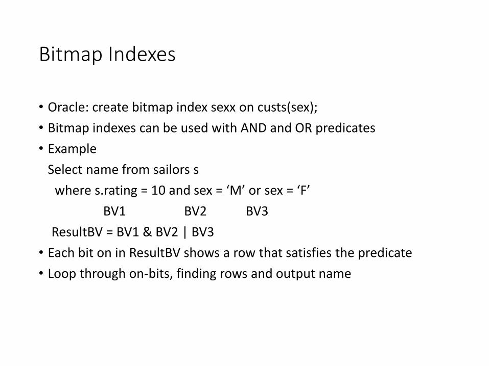
Bitmap Indexes

• Oracle: create bitmap index sexx on custs(sex);

• Bitmap indexes can be used with AND and OR predicates

• Example

Select name from sailors s

where s.rating = 10 and sex = ‘M’ or sex = ‘F’

BV1 BV2 BV3

ResultBV = BV1 & BV2 | BV3

• Each bit on in ResultBV shows a row that satisfies the predicate

• Loop through on-bits, finding rows and output name

Oracle Bitmap index plan

• EXPLAIN PLAN FOR SELECT * FROM t WHERE c1 = 2 AND c2 <> 6 OR c3 BETWEEN 10 AND 20;

•

• EXPLAIN PLAN FOR

• SELECT * FROM t WHERE c1 = 2 AND c2 <> 6 OR c3 BETWEEN 10 AND 20;

• SELECT STATEMENT

• TABLE ACCESS T BY INDEX ROWID

• BITMAP CONVERSION TO ROWID -- get ROWIDs for each on-bit

• BITMAP OR --top level OR

• BITMAP MINUS --to remove null values of c2

• BITMAP MINUS -- to calc c1 = 2 AND c2 <> 6

• BITMAP INDEX C1_IND SINGLE VALUE --c1= 2 BV

• BITMAP INDEX C2_IND SINGLE VALUE --c2 = 6 BV

• BITMAP INDEX C2_IND SINGLE VALUE --c2 = null BV (no not null on col)

• BITMAP MERGE --merge BV’s over C3 range

• BITMAP INDEX C3_IND RANGE SCAN

Bitmaps for star schemas, to be continued

• The dimension tables are not large, maybe 100 rows

• Thus the FK columns in the fact table have only 100 values

• Bitmap indexes can pinpoint rows once determined.

• Bitmaps can be AND’d and OR’d

• Example: time.fiscal_period IN ('3Q95',

'4Q95') matches say 180 days in time table, so 180 FK values in fact’s time_key column

• OR together the 180 bitmaps, get a bitmap locating all fact rows that satisfy this predicate