1

1

Data WarehousingData Warehousing

Decision-Support Systems Data Analysis

OLAP

Extended aggregation features in SQL

– Windowing and ranking

Implementation Techniques

View Materialization

Indexing

2

2

Decision Support SystemsDecision Support Systems

Decision-support systems are used to make business decisions often based on data collected by on-line transaction-processing systems.

Examples of business decisions: what items to stock?

What insurance premium to change?

Who to send advertisements to?

Examples of data used for making decisions Retail sales transaction details

Customer profiles (income, age, sex, etc.)

3

3

Decision-Support Systems: OverviewDecision-Support Systems: Overview

Data analysis tasks are simplified by specialized tools and SQL extensions Example tasks

For each product category and each region, what were the total sales in the last quarter and how do they compare with the same quarter last year

As above, for each product category and each customer category

Statistical analysis packages (e.g., : S++) can be interfaced with databases Statistical analysis is a large field will not study it here

Data mining seeks to discover knowledge automatically in the form of statistical rules and patterns from Large databases.

A data warehouse archives information gathered from multiple sources, and stores it under a unified schema, at a single site. Important for large businesses which generate data from multiple divisions,

possibly at multiple sites Data may also be purchased externally

4

4

Decision-Support Systems: OverviewDecision-Support Systems: Overview

Composed of four major components: Data Store Component

That is, DSS database

Data Extraction and Filtering Component

Used to extract and validate data taken from operational databases and external data sources

End-User Query Tool

Used to create queries that access Data Store Component

End-User Presentation Tool Component

Used to organize and present data

5

5

Main Components of a Main Components of a Decision Support System (DSS)Decision Support System (DSS)

6

6

Transforming Operational Data Into Transforming Operational Data Into Decision Support DataDecision Support Data

7

7

Contrasting Operational and DSS Data Contrasting Operational and DSS Data CharacteristicsCharacteristics

8

8

The Data Warehouse The Data Warehouse Integrated, subject-oriented, time-variant, nonvolatile database

that provides support for decision making Growing industry: $8 billion in 1998 Range from desktop to huge:

Walmart: 900-CPU, 2,700 disk, 23TBTeradata system

Lots of buzzwords, hype slice & dice, rollup, MOLAP, pivot, ...

9

9

What is a Warehouse?What is a Warehouse? Collection of diverse data

subject oriented

aimed at executive, decision maker

often a copy of operational data

with value-added data (e.g., summaries, history)

integrated

time-varying

non-volatile

more

10

10

What is a Warehouse?What is a Warehouse? Collection of tools

gathering data

cleansing, integrating, ...

querying, reporting, analysis

data mining

monitoring, administering warehouse

11

11

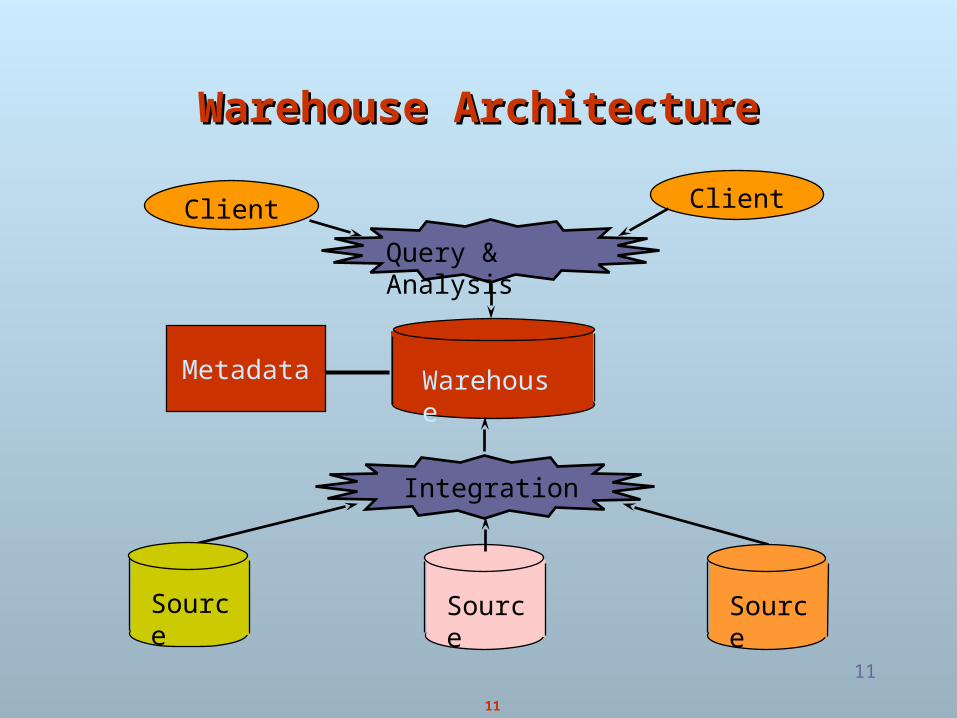
Warehouse ArchitectureWarehouse Architecture

Client Client

Warehouse

Source Source Source

Query & Analysis

Integration

Metadata

12

12

Why a Warehouse?Why a Warehouse? Two Approaches:

Query-Driven (Lazy)

Warehouse (Eager)

Source Source

?

13

13

Query-Driven ApproachQuery-Driven Approach

Client Client

Wrapper Wrapper Wrapper

Mediator

Source Source Source

14

14

Advantages of WarehousingAdvantages of Warehousing High query performance

Queries not visible outside warehouse

Local processing at sources unaffected

Can operate when sources unavailable

Can query data not stored in a DBMS

Extra information at warehouse Modify, summarize (store aggregates)

Add historical information

15

15

Advantages of Query-DrivenAdvantages of Query-Driven No need to copy data

less storage

no need to purchase data

More up-to-date data

Query needs can be unknown

Only query interface needed at sources

16

16

Data MartsData Marts

Smaller warehouses

Spans part of organization e.g., marketing (customers, products, sales)

Do not require enterprise-wide consensus but long term integration problems?

17

17

Creating a Data WarehouseCreating a Data Warehouse

18

18

Data Analysis and OLAPData Analysis and OLAP Aggregate functions summarize large volumes of data

Online Analytical Processing (OLAP) Interactive analysis of data, allowing data to be summarized and

viewed in different ways in an online fashion (with negligible delay)

Data that can be modeled as dimension attributes and measure attributes are called multidimensional data. Given a relation used for data analysis, we can identify some of its

attributes as measure attributes, since they measure some value, and can be aggregated upon. For instance, the attribute number of the sales relation is a measure attribute, since it measures the number of units sold.

Some of the other attributes of the relation are identified as dimension attributes, since they define the dimensions on which measure attributes, and summaries of measure attributes, are viewed.

19

19

Integration of OLAP Integration of OLAP with a Spreadsheet Programwith a Spreadsheet Program

20

20

OLAP Client/Server ArchitectureOLAP Client/Server Architecture

21

21

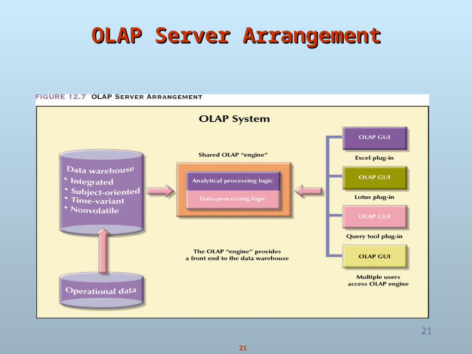
OLAP Server ArrangementOLAP Server Arrangement

22

22

OLAP Server with Multidimensional Data OLAP Server with Multidimensional Data Store ArrangementStore Arrangement

23

23

OLAP Server With Local Mini Data MartsOLAP Server With Local Mini Data Marts

24

24

OLAP ImplementationOLAP Implementation The earliest OLAP systems used multidimensional arrays in

memory to store data cubes, and are referred to as multidimensional OLAP (MOLAP) systems.

OLAP implementations using only relational database features are called relational OLAP (ROLAP) systems

Hybrid systems, which store some summaries in memory and store the base data and other summaries in a relational database, are called hybrid OLAP (HOLAP) systems.

25

25

Typical ROLAP Client/Server Typical ROLAP Client/Server ArchitectureArchitecture

26

26

MOLAP Client/Server ArchitectureMOLAP Client/Server Architecture

27

27

Relational vs. Multidimensional OLAPRelational vs. Multidimensional OLAP

28

28

Warehouse SchemasWarehouse Schemas Typically warehouse data is multidimensional, with very large

fact tables Examples of dimensions: item-id, date/time of sale, store where sale

was made, customer identifier

Examples of measures: number of items sold, price of items

Dimension values are usually encoded using small integers and mapped to full values via dimension tables Resultant schema is called a star schema

More complicated schema structures

– Snowflake schema: multiple levels of dimension tables

– Constellation: multiple fact tables

29

29

StarStar

customer custId name address city53 joe 10 main sfo81 fred 12 main sfo

111 sally 80 willow la

product prodId name pricep1 bolt 10p2 nut 5

store storeId cityc1 nycc2 sfoc3 la

sale oderId date custId prodId storeId qty amto100 1/7/97 53 p1 c1 1 12o102 2/7/97 53 p2 c1 2 11105 3/8/97 111 p1 c3 5 50

30

30

Star SchemaStar Schema

saleorderId

datecustIdprodIdstoreId

qtyamt

customercustIdname

addresscity

productprodIdnameprice

storestoreId

city

31

31

TermsTerms Fact table

Dimension tables

Measures

saleorderId

datecustIdprodIdstoreId

qtyamt

customercustIdname

addresscity

productprodIdnameprice

storestoreId

city

32

32

Star SchemasStar Schemas

A star schema is a common organization for data at a warehouse. It consists of:

1. Fact table : a very large accumulation of facts such as sales.

Often “insert-only.”

2. Dimension tables : smaller, generally static information about the entities involved in the facts.

33

33

Dimension HierarchiesDimension Hierarchies

store storeId cityId tId mgrs5 sfo t1 joes7 sfo t2 freds9 la t1 nancy

city cityId pop regIdsfo 1M northla 5M south

region regId namenorth cold regionsouth warm region

sType tId size locationt1 small downtownt2 large suburbs

storesType

city region

snowflake schema constellations

34

34

Online Analytical ProcessingOnline Analytical Processing The operation of changing the dimensions used in a cross-tab is

called pivoting

Suppose an analyst wishes to see a cross-tab on item-name and color for a fixed value of size, for example, large, instead of the sum across all sizes.

Such an operation is referred to as slicing. The operation is sometimes called dicing, particularly when

values for multiple dimensions are fixed.

The operation of moving from finer-granularity data to a coarser granularity is called a rollup.

The opposite operation - that of moving from coarser-granularity data to finer-granularity data – is called a drill down.

35

35

Three-Dimensional Data CubeThree-Dimensional Data Cube A data cube is a multidimensional generalization of a crosstab

Cannot view a three-dimensional object in its entirety but crosstabs can be used as views on a data cube

36

36

CubeCube

sale prodId storeId amtp1 c1 12p2 c1 11p1 c3 50p2 c2 8

c1 c2 c3p1 12 50p2 11 8

Fact table view: Multi-dimensional cube:

dimensions = 2

37

37

3-D Cube3-D Cube

sale prodId storeId date amtp1 c1 1 12p2 c1 1 11p1 c3 1 50p2 c2 1 8p1 c1 2 44p1 c2 2 4

day 2c1 c2 c3

p1 44 4p2 c1 c2 c3

p1 12 50p2 11 8

day 1

dimensions = 3

Multi-dimensional cube:Fact table view:

38

38

Typical OLAP QueriesTypical OLAP Queries Often, OLAP queries begin with a “star join”: the natural join of the fact

table with all or most of the dimension tables. The typical OLAP query will:

1. Start with a star join.

2. Select for interesting tuples, based on dimension data.

3. Group by one or more dimensions.

4. Aggregate certain attributes of the result.

39

39

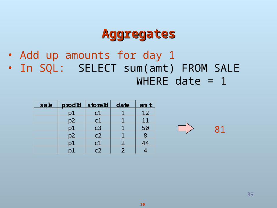
AggregatesAggregates

sale prodId storeId date amtp1 c1 1 12p2 c1 1 11p1 c3 1 50p2 c2 1 8p1 c1 2 44p1 c2 2 4

• Add up amounts for day 1• In SQL: SELECT sum(amt) FROM SALE WHERE date = 1

81

40

40

AggregatesAggregates

sale prodId storeId date amtp1 c1 1 12p2 c1 1 11p1 c3 1 50p2 c2 1 8p1 c1 2 44p1 c2 2 4

• Add up amounts by day• In SQL: SELECT date, sum(amt) FROM SALE GROUP BY date

ans date sum1 812 48

41

41

Another ExampleAnother Example

sale prodId storeId date amtp1 c1 1 12p2 c1 1 11p1 c3 1 50p2 c2 1 8p1 c1 2 44p1 c2 2 4

• Add up amounts by day, product• In SQL: SELECT date, sum(amt) FROM SALE GROUP BY date, prodId

sale prodId date amtp1 1 62p2 1 19p1 2 48

drill-down

rollup

42

42

AggregatesAggregates Operators: sum, count, max, min, median,

ave

“Having” clause

Using dimension hierarchy average by region (within store)

maximum by month (within date)

43

43

Cube AggregationCube Aggregation

day 2c1 c2 c3

p1 44 4p2 c1 c2 c3

p1 12 50p2 11 8

day 1

c1 c2 c3p1 56 4 50p2 11 8

c1 c2 c3sum 67 12 50

sump1 110p2 19

129

. . .

drill-down

rollup

Example: computing sums

44

44

Cube OperatorsCube Operators

day 2c1 c2 c3

p1 44 4p2 c1 c2 c3

p1 12 50p2 11 8

day 1

c1 c2 c3p1 56 4 50p2 11 8

c1 c2 c3sum 67 12 50

sump1 110p2 19

129

. . .

sale(c1,*,*)

sale(*,*,*)sale(c2,p2,*)

45

45

c1 c2 c3 *p1 56 4 50 110p2 11 8 19* 67 12 50 129

Extended CubeExtended Cube

day 2 c1 c2 c3 *p1 44 4 48p2* 44 4 48

c1 c2 c3 *p1 12 50 62p2 11 8 19* 23 8 50 81

day 1

*

sale(*,p2,*)

46

46

Aggregation Using HierarchiesAggregation Using Hierarchies

day 2c1 c2 c3

p1 44 4p2 c1 c2 c3

p1 12 50p2 11 8

day 1

region A region Bp1 56 54p2 11 8

customer

region

country

(customer c1 in Region A;customers c2, c3 in Region B)

47

47

PivotingPivoting

sale prodId storeId date amtp1 c1 1 12p2 c1 1 11p1 c3 1 50p2 c2 1 8p1 c1 2 44p1 c2 2 4

day 2c1 c2 c3

p1 44 4p2 c1 c2 c3

p1 12 50p2 11 8

day 1

Multi-dimensional cube:Fact table view:

c1 c2 c3p1 56 4 50p2 11 8

48

48

OLAP Implementation OLAP Implementation Early OLAP systems precomputed all possible aggregates in order

to provide online response Space and time requirements for doing so can be very high

2n combinations of group by

It suffices to precompute some aggregates, and compute others on demand from one of the precomputed aggregates Can compute aggregate on (item-name, color) from an aggregate

on (item-name, color, size)

– For all but a few “non-decomposable” aggregates such as median

– is cheaper than computing it from scratch

Several optimizations available for computing multiple aggregates Can compute aggregate on (item-name, color) from an aggregate on

(item-name, color, size) Can compute aggregates on (item-name, color, size),

(item-name, color) and (item-name) using a single sorting of the base data

49

49

Cross Tabulation of Cross Tabulation of salessales by by item-name item-name and and colorcolor

The table above is an example of a cross-tabulation (cross-tab), also referred to as a pivot-table.

A cross-tab is a table where values for one of the dimension attributes form the row headers, values

for another dimension attribute form the column headers Other dimension attributes are listed on top

Values in individual cells are (aggregates of) the values of the dimension attributes that specify the cell.

50

50

Relational Representation of CrosstabsRelational Representation of Crosstabs

Crosstabs can be represented as relations The value all is used to

represent aggregates The SQL:1999 standard

actually uses null values in place of all More on this later….

51

51

Hierarchies on DimensionsHierarchies on Dimensions Hierarchy on dimension attributes: lets dimensions to be viewed

at different levels of detail E.g. the dimension DateTime can be used to aggregate by hour of

day, date, day of week, month, quarter or year

52

52

Cross Tabulation With HierarchyCross Tabulation With Hierarchy

Crosstabs can be easily extended to deal with hierarchies Can drill down or roll up on a hierarchy

53

53

Extended AggregationExtended Aggregation SQL-92 aggregation quite limited

Many useful aggregates are either very hard or impossible to specify

Data cube

Complex aggregates (median, variance)

binary aggregates (correlation, regression curves)

ranking queries (“assign each student a rank based on the total marks”

SQL:1999 OLAP extensions provide a variety of aggregation functions to address above limitations Supported by several databases, including Oracle and IBM DB2

54

54

Extended Aggregation in SQL:1999Extended Aggregation in SQL:1999 The cube operation computes union of group by’s on every subset

of the specified attributes

E.g. consider the query

select item-name, color, size, sum(number)from salesgroup by cube(item-name, color, size)

This computes the union of eight different groupings of the sales relation:

{ (item-name, color, size), (item-name, color), (item-name, size), (color, size), (item-name), (color), (size), ( ) }

where ( ) denotes an empty group by list.

For each grouping, the result contains the null value for attributes not present in the grouping.

55

55

Extended Aggregation (Cont.)Extended Aggregation (Cont.) Relational representation of crosstab that we saw earlier, but with null in

place of all, can be computed by

select item-name, color, sum(number)from salesgroup by cube(item-name, color)

The function grouping() can be applied on an attribute Returns 1 if the value is a null value representing all, and returns 0 in all other

cases.

select item-name, color, size, sum(number),grouping(item-name) as item-name-flag,grouping(color) as color-flag,grouping(size) as size-flag,

from salesgroup by cube(item-name, color, size)

Can use the function decode() in the select clause to replace such nulls by a value such as all

E.g. replace item-name in first query by decode( grouping(item-name), 1, ‘all’, item-name)

56

56

Extended Aggregation (Cont.)Extended Aggregation (Cont.) The rollup construct generates union on every prefix of specified list of

attributes E.g.

select item-name, color, size, sum(number)from salesgroup by rollup(item-name, color, size)

Generates union of four groupings:

{ (item-name, color, size), (item-name, color), (item-name), ( ) } Rollup can be used to generate aggregates at multiple levels of a

hierarchy. E.g., suppose table itemcategory(item-name, category) gives the

category of each item. Then

select category, item-name, sum(number) from sales, itemcategory where sales.item-name = itemcategory.item-name group by rollup(category, item-name)

would give a hierarchical summary by item-name and by category.

57

57

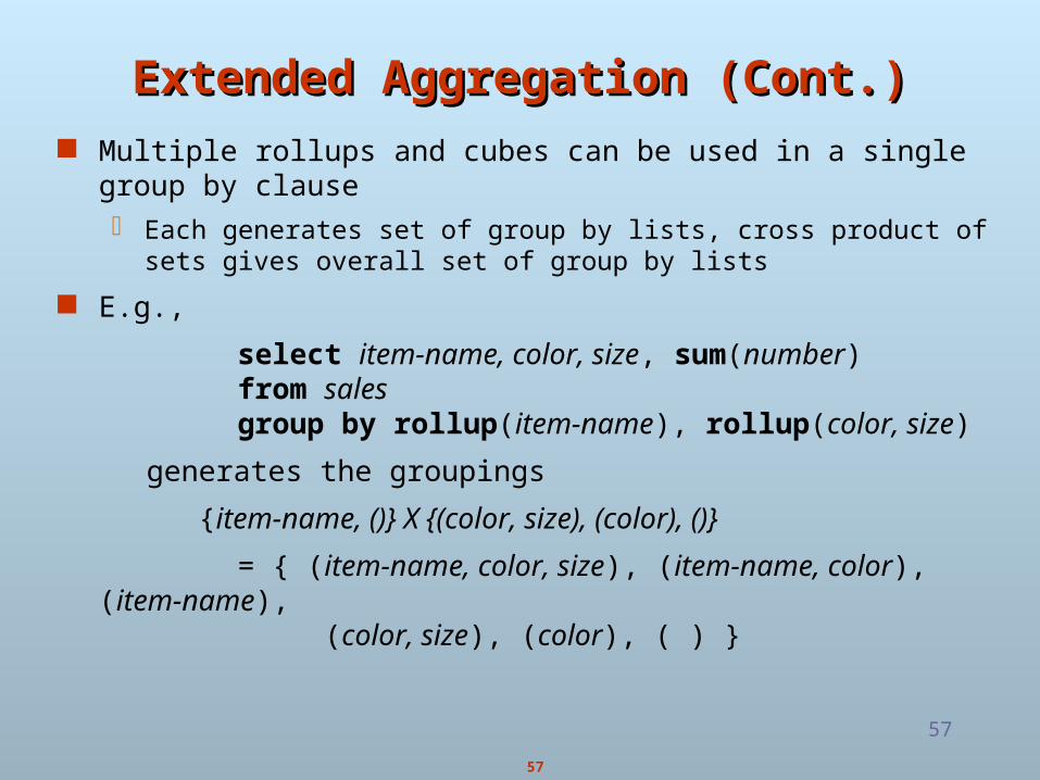
Extended Aggregation (Cont.)Extended Aggregation (Cont.) Multiple rollups and cubes can be used in a single group by clause

Each generates set of group by lists, cross product of sets gives overall set of group by lists

E.g.,

select item-name, color, size, sum(number) from sales group by rollup(item-name), rollup(color, size)

generates the groupings

{item-name, ()} X {(color, size), (color), ()}

= { (item-name, color, size), (item-name, color), (item-name), (color, size), (color), ( ) }

58

58

RankingRanking Ranking is done in conjunction with an order by specification.

Given a relation student-marks(student-id, marks) find the rank of each student.

select student-id, rank( ) over (order by marks desc) as s-rankfrom student-marks

An extra order by clause is needed to get them in sorted order

select student-id, rank ( ) over (order by marks desc) as s-rankfrom student-marks order by s-rank

Ranking may leave gaps: e.g. if 2 students have the same top mark, both have rank 1, and the next rank is 3 dense_rank does not leave gaps, so next dense rank would be 2

59

59

Ranking (Cont.)Ranking (Cont.) Ranking can be done within partition of the data.

“Find the rank of students within each section.”

select student-id, section,rank ( ) over (partition by section order by marks desc)

as sec-rankfrom student-marks, student-sectionwhere student-marks.student-id = student-section.student-idorder by section, sec-rank

Multiple rank clauses can occur in a single select clause

Ranking is done after applying group by clause/aggregation

Exercises: Find students with top n ranks

Many systems provide special (non-standard) syntax for “top-n” queries

Rank students by sum of their marks in different courses

given relation student-course-marks(student-id, course, marks)

60

60

Ranking (Cont.)Ranking (Cont.) Other ranking functions:

percent_rank (within partition, if partitioning is done)

cume_dist (cumulative distribution)

fraction of tuples with preceding values

row_number (non-deterministic in presence of duplicates)

SQL:1999 permits the user to specify nulls first or nulls last

select student-id, rank ( ) over (order by marks desc nulls last) as s-rankfrom student-marks

61

61

Ranking (Cont.)Ranking (Cont.) For a given constant n, the ranking the function ntile(n) takes the

tuples in each partition in the specified order, and divides them into n buckets with qual numbers of tuples. For instance, we an sort employees by salary, and use ntile(3) to find which range (bottom third, middle third, or top third) each employee is in, and compute the total salary earned by employees in each range:

select threetile, sum(salary)from (

select salary, ntile(3) over (order by salary) as threetilefrom employee) as s

group by threetile

62

62

WindowingWindowing E.g.: “Given sales values for each date, calculate for each date the average of

the sales on that day, the previous day, and the next day” Such moving average queries are used to smooth out random variations. In contrast to group by, the same tuple can exist in multiple windows Window specification in SQL:

Ordering of tuples, size of window for each tuple, aggregate function E.g. given relation sales(date, value)

select date, sum(value) over (order by date between rows 1 preceding and 1 following) from sales

Examples of other window specifications: between rows unbounded preceding and current rows unbounded preceding range between 10 preceding and current row

All rows with values between current row value –10 to current value range interval 10 day preceding

Not including current row

63

63

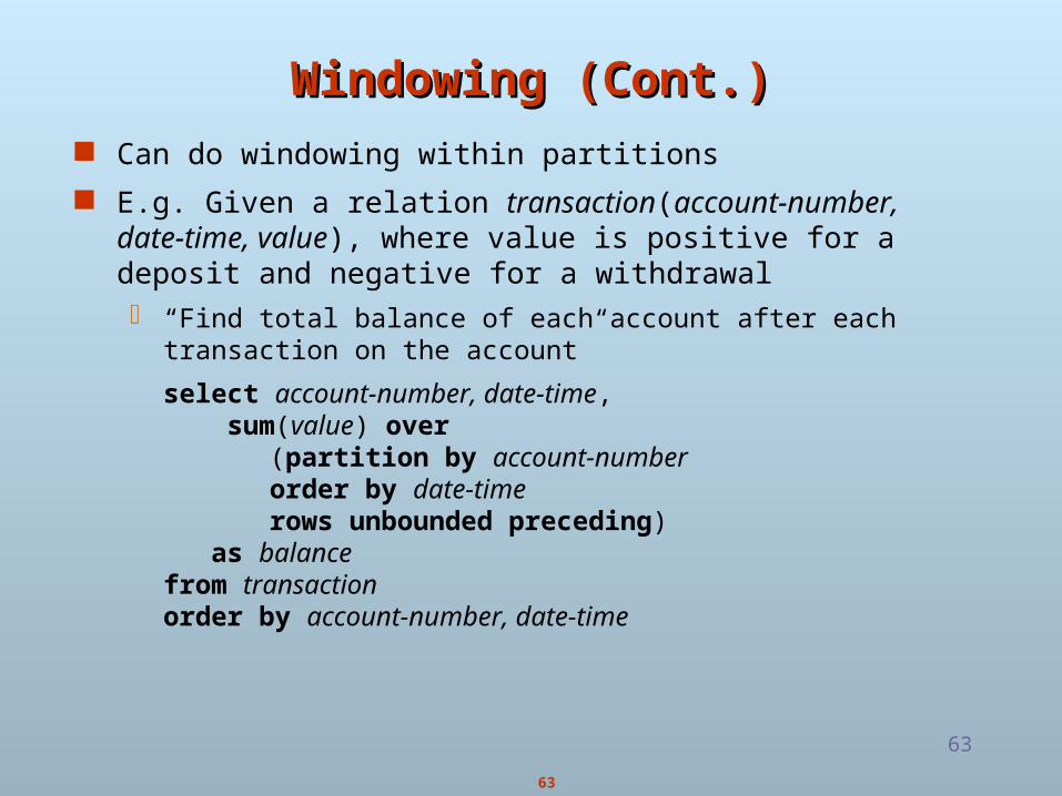
Windowing (Cont.)Windowing (Cont.) Can do windowing within partitions

E.g. Given a relation transaction(account-number, date-time, value), where value is positive for a deposit and negative for a withdrawal “Find total balance of each account after each transaction on the

account”

select account-number, date-time, sum(value) over

(partition by account-number order by date-timerows unbounded preceding)

as balancefrom transactionorder by account-number, date-time