Data-moderate stock assessments for brown, China, copper

Data-moderate stock assessments for brown, China, copper, sharpchin,

stripetail, and yellowtail rockfishes and English and rex soles in 2013

by

Jason Cope1, E.J. Dick2, Alec MacCall2, Melissa Monk2, Braden Soper2, and Chantell Wetzel1

January 2015

1Northwest Fisheries Science Center U.S. Department of Commerce

National Oceanic and Atmospheric Administration National Marine Fisheries Service

2725 Montlake Boulevard East Seattle, Washington 98112-2097

2Southwest Fisheries Science Center

U.S. Department of Commerce National Oceanic and Atmospheric Administration

National Marine Fisheries Service 110 Shaffer Rd

Santa Cruz, CA 95060

1

Table of Contents

Executive Summary ............................................................................................ 4 Stocks ......................................................................................................................... 4 Derived outputs ......................................................................................................... 4 Decision tables .......................................................................................................... 5

Nearshore rockfishes ............................................................................................... 5 Shelf-slope stocks .................................................................................................. 11

1 Introduction ................................................................................................ 16 1.1 Biology, Ecology, and Life History .............................................................. 16

1.1.1 Nearshore rockfishes ............................................................................... 16 1.1.2 Shelf and Slope Rockfishes ..................................................................... 17 1.1.3 Flatfishes ................................................................................................. 18

2 Assessment ................................................................................................ 18 2.1 Data and Inputs ............................................................................................. 18

2.1.1 Removal histories .................................................................................... 18 2.1.2 Catch data sources .................................................................................. 19 2.1.3 Species removals by fishery, region, and data source .............................. 22 2.1.4 Fishery-independent surveys ................................................................... 23 2.1.5 Fishery-dependent indices ....................................................................... 25

2.2 History of Modeling Approaches ................................................................. 34 2.2.1 Previous assessments ............................................................................. 34

2.3 Model Description ......................................................................................... 35 2.3.1 Bayesian Stock Reduction Analysis (Extended Depletion-Based Stock Reduction Analysis, XDB-SRA) .............................................................................. 35 2.3.2 Extended Simple Stock Synthesis (exSSS) .............................................. 37

2.4 Response to STAR Panel Recommendations ............................................. 39 2.5 Base-Models, Uncertainty and Sensitivity Analyses .................................. 39

2.5.1 XDB-SRA assessments (Fishery-dependent indices only) ....................... 39 2.5.2 ExSSS assessments (Fishery-independent indices only) ......................... 45 2.5.3 Status-Only Assessment .......................................................................... 48

3 Harvest Projections and Decision Tables ................................................ 48

4 Research Needs ......................................................................................... 49

5 Acknowledgments ...................................................................................... 50

6 Literature Cited ........................................................................................... 50

7 Tables .......................................................................................................... 53 7.1 Model data and inputs .................................................................................. 53

7.1.1 Life histories ............................................................................................. 53 7.1.2 Removals ................................................................................................. 54 7.1.3 Surveys .................................................................................................... 79

7.2 Model results ................................................................................................. 97 7.2.1 XBD-SRA model estimates ...................................................................... 97 7.2.2 ExSSS model estimates ......................................................................... 117 7.2.3 Decision tables ....................................................................................... 124

8 Figures ...................................................................................................... 133 8.1 Catch and Abundance Figures ................................................................... 133

2

8.1.1 Distribution maps ................................................................................... 133 8.1.2 Removal histories .................................................................................. 145 8.1.3 Indices of abundance ............................................................................. 153

8.2 Model Results and Diagnostic Figures ...................................................... 178 8.2.1 Brown rockfish ....................................................................................... 178 8.2.2 China rockfish ........................................................................................ 181 8.2.3 Copper rockfish ...................................................................................... 187 8.2.4 Sharpchin rockfish.................................................................................. 193 8.2.5 Yellowtail rockfish (North of 40° 10’ N lat.) ............................................. 206 8.2.6 English sole............................................................................................ 220 8.2.7 Rex sole ................................................................................................. 234 8.2.8 Stripetail rockfish .................................................................................... 247

Appendix ......................................................................................................... 248

Appendix A. SS Files ...................................................................................... 248 Appendix A.1. Sharpchin rockfish ........................................................................ 248 Appendix A.2. Stripetail rockfish .......................................................................... 254 Appendix A.3. Yellowtail rockfish (North of 40° 10′ N lat.) .................................. 260 Appendix A.4. English sole ................................................................................... 267 Appendix A.5. Rex sole ......................................................................................... 274

Appendix B. XDB-SRA Files .......................................................................... 281 Appendix B.1. Brown rockfish .............................................................................. 281 Appendix B.2. China rockfish, South of Cape Mendocino .................................. 284 Appendix B.3. China rockfish, North of Cape Mendocino .................................. 288 Appendix B.4. Copper rockfish, South of Point Conception .............................. 291 Appendix B.5. Copper rockfish, North of Point Conception ............................... 293

Appendix C. Partitioning OFLs for brown and copper rockfish ................. 297 Appendix C.1. Brown rockfish .............................................................................. 297 Appendix C.2. Copper rockfish ............................................................................. 298

3

Executive Summary Stocks The catch and index only stock assessment methods (XDB-SRA and exSSS) were applied to eight species of groundfishes. Six were rockfishes (three nearshore and three shelf and/or slope species) and two flatfishes. Two of the nearshore rockfishes (China and copper) assessments defined and assessed stocks in two areas, the former north and south of Cape Mendocino, CA and the latter north and south of Point Conception, CA. Yellowtail rockfish was also considered as two stocks north and south of Cape Mendocino, but only the northern stock was assessed. The remaining rockfishes and two flatfishes were treated as coastwide stocks. Derived outputs All stocks were found to be above the biomass limit reference points. No stocks were therefore found to be overfished, but at least one (China rockfish north) is below the target reference point. Overfishing may also be occurring on that stock. Estimated population biomass of the nearshore rockfishes with assessments using fishery-dependent data demonstrated less uncertainty than the shelf and slope species with assessments using fishery-independent survey data. Overall exploitation rates were smaller than that estimated by FMSY. Given the high stock status of the shelf-slope species, the estimated OFLs are high and well above average catch over the last 3 years. Table ES1. Derived outputs for each assessed stock. Central tendency is reported as the median. Numbers in parentheses are 95% credibility intervals. * OFL estimates for Copper rockfish North and South of 40°10′ N. lat. are a post-stratification of assessment results based on cumulative removals by area, 1916-2012.

Model Group Stock Area SB0 SB2013 SB2013/SB0 SBMSY

XDB-SRA Rockfishes Brown rockfish Coastwide 1794 (977 - 3732) 727 (333 - 2285) 0.42 (0.22 - 0.77) 718 (391 - 1493)XDB-SRA Rockfishes China rockfish N. of 40°10' N lat. 243 (127 - 542) 84 (22 - 366) 0.37 (0.12 - 0.73) 97 (51 - 217)XDB-SRA Rockfishes China rockfish S. of 40°10' N lat. 405 (232 - 1272) 264 (138 - 925) 0.66 (0.4 - 0.93) 162 (93 - 509)XDB-SRA Rockfishes Copper rockfish N. of 34°27' N lat. 1704 (1081 - 2734) 795 (417 - 1694) 0.48 (0.26 - 0.85) 681 (433 - 1093)XDB-SRA Rockfishes Copper rockfish S. of 34°27' N lat. 942 (545 - 2745) 699 (351 - 2189) 0.76 (0.43 - 0.99) 377 (218 - 1098)exSSS AIS Rockfishes Sharpchin Coastwide 7887 (2437-24724) 4947 (1456-21157) 0.680 (0.31-0.91) 1944 (634-6509)exSSS AIS Rockfishes Yellowtail (N) N. of 40°10' N lat. 82974 (19363-277492) 50043 (12184-221920) 0.667 (0.35-0.90) 19020 (4617-70550)exSSS AIS Flatfishes English sole Coastwide 29238 (11757-94321) 25719(10444-89100) 0.879 (0.77-0.96) 4898 (1019-18983)exSSS AIS Flatfishes Rex sole Coastwide 3808 (731-15814) 2966 (602-13150) 0.800 (0.64-0.93) 560 (255-3418)

Model Group Stock F2012/FMSY MSY OFL2015 OFL2016

XDB-SRA Rockfishes Brown rockfish Coastwide 0.63 (0.27 - 1.47) 149 (109 - 196) 166 (69 - 364) 162 (66 - 361)XDB-SRA Rockfishes China rockfish N. of 40°10' N lat. 2.15 (0.49 - 11.29) 9 (3 - 20) 7 (1 - 35) 7 (1 - 36)XDB-SRA Rockfishes China rockfish S. of 40°10' N lat. 0.27 (0.13 - 0.58) 32 (22 - 50) 55 (25 - 108) 53 (23 - 104)XDB-SRA Rockfishes Copper rockfish N. of 34°27' N lat. 0.34 (0.15 - 0.87) 114 (75 - 148) 145 (56 - 314) 141 (52 - 308)XDB-SRA Rockfishes Copper rockfish S. of 34°27' N lat. 0.32 (0.16 - 0.86) 84 (51 - 136) 167 (59 - 303) 154 (54 - 287)XDB-SRA Rockfishes Copper rockfish N. of 40°10' N lat. -- -- 11* 10*XDB-SRA Rockfishes Copper rockfish S. of 40°10' N lat. -- -- 301* 284*exSSS AIS Rockfishes Sharpchin Coastwide 0.02 320 (154-883) 416 (130-1474) 404 (132-1397)exSSS AIS Rockfishes Yellowtail rockfish N. of 40°10' N lat. 0.11 5728 (3295-14517) 7218 (2646-23903) 6949 (2679-22724)exSSS AIS Flatfishes English sole Coastwide 0.013 4072 (3210-11847) 10792 (7138-32391) 7890 (4921-23317)exSSS AIS Flatfishes Rex sole Coastwide 0.07 1676 (1230-3622) 5764 (3089-16500) 3956 (2479-10253)

Derived Outputs: Scale and Status

Derived Outputs: Fishing and Removals

4

Decision tables Forecasts for each stock are based on a 12-year outlook predicated on one of two control rules: 1) constant catch based on the average of the last three years or landings and 2) catch based on the P* OFL buffer and the “40-10” ABC control rule. The latter has three catch scenarios based on the forecasted results of the three states of nature. These states of nature capture different states in depletion by taking the median value of starting depletion and resultant median forecasted catch under control rule 2 above and the base case model for the following portions of the posterior depletion distribution: 1) bottom quartile of starting depletion values, 2) interquartile of the starting depletion, and 3) upper quartile of the starting depletion. Thus 25% of the distribution is in each of the lower and upper states of nature, with 50% contained in the middle state. A total of three models were therefore run with the three different catch scenarios based on control rule #2, then each state of nature (posterior density quartiles) was summarized by the median value of the draws contained in that state of nature. Each forecast assumes full attainment of the prescribed catch and no implementation error. Nearshore rockfishes Decision tables for the nearshore rockfish stock assessments are given in Tables ES2 through ES6 (Post-STAR panel base case only). See Tables 65-69 for alternative states of nature presented during the STAR Panel. Differences between Tables 65-69 and the final base case (Tables ES2-ES6) are minor, and qualitative patterns among alternative states of nature remain unchanged.

5

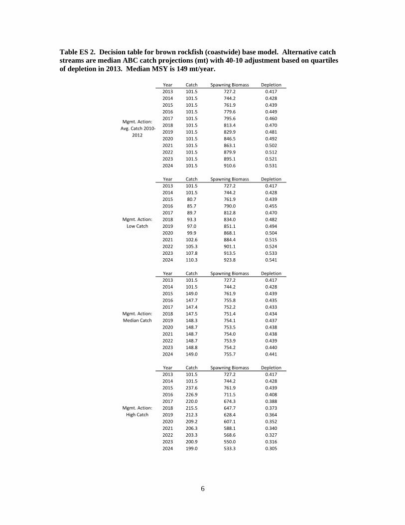
Table ES 2. Decision table for brown rockfish (coastwide) base model. Alternative catch streams are median ABC catch projections (mt) with 40-10 adjustment based on quartiles of depletion in 2013. Median MSY is 149 mt/year.

Year Catch Spawning Biomass Depletion2013 101.5 727.2 0.4172014 101.5 744.2 0.4282015 101.5 761.9 0.4392016 101.5 779.6 0.4492017 101.5 795.6 0.4602018 101.5 813.4 0.4702019 101.5 829.9 0.4812020 101.5 846.5 0.4922021 101.5 863.1 0.5022022 101.5 879.9 0.5122023 101.5 895.1 0.5212024 101.5 910.6 0.531




Mgmt. Action: Avg. Catch 2010-

2012

Mgmt. Action: Low Catch

Mgmt. Action: Median Catch

Mgmt. Action: High Catch

6

Table ES3. Decision table for China rockfish (north of 40° 10′ N lat.) base model. Alternative catch streams are median ABC catch projections (mt) with 40-10 adjustment based on quartiles of depletion in 2013. Median MSY is 9 mt/year.








2012


7

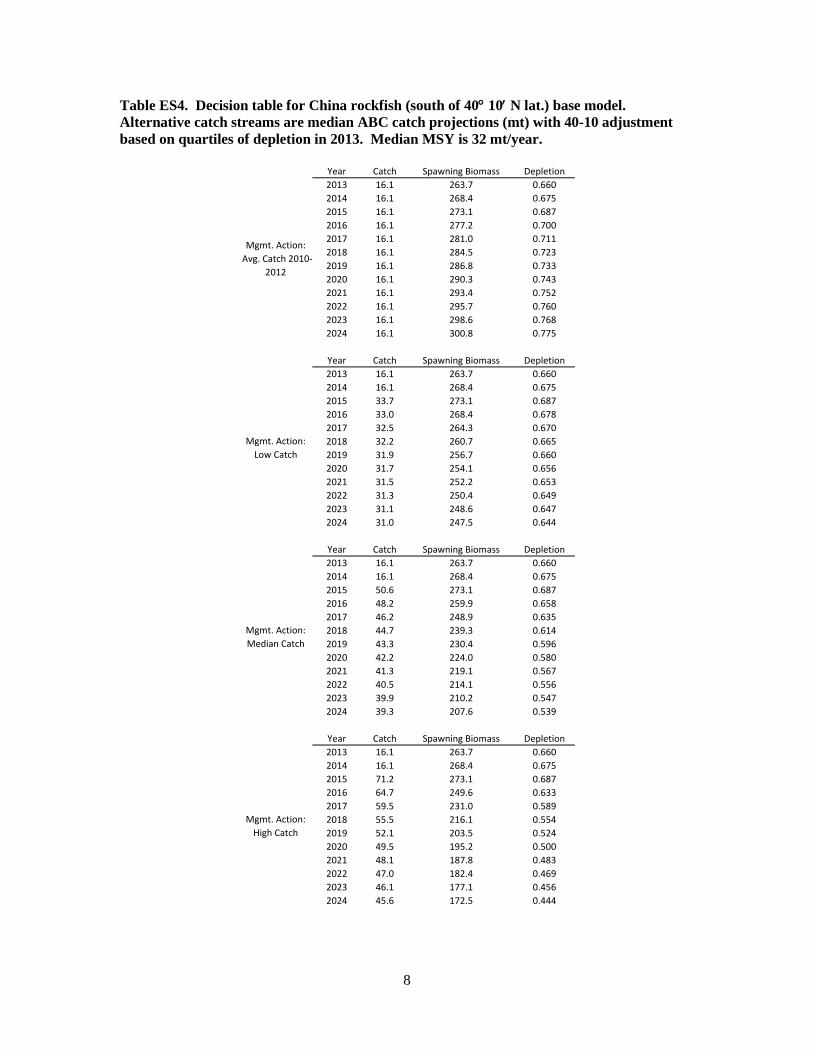
Table ES4. Decision table for China rockfish (south of 40° 10′ N lat.) base model. Alternative catch streams are median ABC catch projections (mt) with 40-10 adjustment based on quartiles of depletion in 2013. Median MSY is 32 mt/year.






2012




8

Table ES5. Decision table for copper rockfish (north of 34° 27′ N lat.) base model. Alternative catch streams are median ABC catch projections (mt) with 40-10 adjustment based on quartiles of depletion in 2013. Median MSY is 114 mt/year.






2012




9

Table ES6. Decision table for copper rockfish (south of 34° 27′ N lat.). Alternative catch streams are median ABC catch projections (mt) with 40-10 adjustment based on quartiles of depletion in 2013. Median MSY is 84 mt/year.






2012




10

Shelf-slope stocks Results for the shelf-slope fishery-independent stock assessments are provided in Tables ES7 through ES10. The average catch scenarios increase the stock biomass, and thus status, of all stocks in all states of nature relative to the other catch scenarios modeled. The high catch scenarios drop stock status below the target reference point in the base depletion state of nature by the end of the 12 year forecast for all four stocks. The rockfishes also drop below the limit reference point in the low depletion state of nature under the high catch scenario.

11

Table ES7. Decision table for sharpchin rockfish. Alternative catch streams are median ABC catch projections (mt) with 40-10 adjustment based on quartiles of depletion in 2013. “Spawning Biomass” is median female spawning stock biomass. “Depletion” is median depletion. Estimated MSY is 320 mt/year and the long-term average total yield based on SPR50% is 270 mt/year. .

Year CatchSpawning Biomass Depletion

Spawning Biomass Depletion


2015 195 3,485 51.5% 5,798 71.8% 7,904 86.3%2016 195 3,476 51.2% 5,791 71.6% 7,894 85.8%2017 194 3,469 50.9% 5,779 71.3% 7,881 85.4%2018 194 3,447 50.7% 5,762 71.1% 7,867 85.0%2019 193 3,440 50.4% 5,752 70.9% 7,852 84.8%2020 192 3,431 50.1% 5,743 70.6% 7,831 84.5%2021 191 3,426 49.9% 5,724 70.4% 7,798 84.2%2022 190 3,418 49.7% 5,705 70.2% 7,769 84.1%2023 189 3,401 49.5% 5,685 69.9% 7,744 83.8%2024 189 3,395 49.3% 5,667 69.8% 7,721 83.6%2015 382 3,371 51.1% 5,628 71.2% 7,561 86.0%2016 372 3,393 50.6% 5,531 69.5% 7,216 82.2%2017 363 3,394 50.1% 5,426 67.8% 6,908 78.4%2018 354 3,380 49.6% 5,300 66.1% 6,570 75.2%2019 347 3,377 49.2% 5,177 64.3% 6,313 72.5%2020 339 3,365 49.0% 5,091 62.7% 6,094 69.9%2021 334 3,363 48.6% 4,984 61.5% 5,895 67.5%2022 328 3,347 48.5% 4,933 60.4% 5,720 65.4%2023 322 3,321 48.3% 4,840 59.4% 5,561 63.8%2024 317 3,336 48.2% 4,770 58.5% 5,419 62.2%2015 750 3,343 50.6% 5,688 71.7% 7,863 86.0%2016 730 2,964 44.1% 5,338 66.4% 7,567 82.3%2017 703 2,594 38.6% 4,999 61.8% 7,310 87.7%2018 674 2,257 33.6% 4,643 57.2% 7,040 75.7%2019 650 1,953 28.9% 4,300 53.3% 6,791 73.1%2020 625 1,684 24.7% 4,001 49.6% 6,498 70.5%2021 612 1,392 20.8% 3,691 46.7% 6,215 68.6%2022 591 1,190 17.1% 3,479 43.6% 6,055 66.7%2023 575 980 13.9% 3,266 41.0% 5,935 65.0%2024 563 756 10.9% 3,095 38.6% 5,816 63.5%2015 5 3,485 50.6% 5,664 72.0% 7,573 86.4%2016 5 3,602 51.9% 5,786 73.4% 7,643 87.4%2017 5 3,725 53.7% 5,895 74.7% 7,708 88.2%2018 5 3,826 54.9% 6,020 75.9% 7,768 89.0%2019 5 3,938 56.3% 6,121 77.0% 7,828 89.7%2020 5 4,042 57.7% 6,227 78.3% 7,888 90.3%2021 5 4,135 59.0% 6,327 79.3% 7,944 91.1%2022 5 4,260 60.4% 6,420 80.3% 7,998 91.6%2023 5 4,318 61.6% 6,510 81.2% 8,048 92.2%2024 5 4,418 62.6% 6,599 82.2% 8,096 92.8%

0.25-0.75 0.75-1.0

State of nature

Low Catches

Medium Catches

High Catches

Average Catches

Low Base HighQuantiles 0-0.25

12

Table ES8. Decision table for yellowtail rockfish (north of 40° 10′ N lat.). Alternative catch streams are median ABC catch projections (mt) with 40-10 adjustment based on quartiles of depletion in 2013. “Spawning Biomass” is median female spawning stock biomass. “Depletion” is median depletion. Estimated MSY is 5728 mt/year and the long-term average total yield based on SPR50% is 4805 mt/year. .




2015 3,936 43,502 52.8% 56,604 68.9% 62,979 83.4%2016 3,912 43,108 52.4% 56,063 68.3% 62,573 82.7%2017 3,879 42,738 52.0% 55,772 67.9% 62,187 81.9%2018 3,844 42,434 51.7% 55,468 67.4% 61,835 81.2%2019 3,818 42,206 51.3% 55,027 66.7% 61,524 80.6%2020 3,797 41,976 50.9% 54,624 66.4% 61,253 79.9%2021 3,777 41,749 50.6% 54,269 66.0% 61,019 79.6%2022 3,759 41,547 50.4% 53,958 65.7% 60,818 79.3%2023 3,744 41,393 50.1% 53,684 65.3% 60,644 79.0%2024 3,730 41,129 50.0% 53,444 64.9% 60,491 78.8%

6,497 43,502 52.4% 54,304 69.3% 60,039 83.3%2016 6,312 43,252 52.1% 52,730 66.8% 55,750 87.0%2017 6,126 43,044 51.6% 51,060 64.6% 52,853 73.9%2018 5,962 42,955 51.1% 49,531 62.7% 50,294 70.5%2019 5,798 42,673 50.7% 48,227 61.0% 48,062 67.2%2020 5,638 42,597 50.4% 47,111 49.4% 46,136 64.4%2021 5,523 42,567 50.0% 46,260 58.2% 44,484 62.3%2022 5,417 42,547 49.9% 45,421 57.1% 43,067 60.5%2023 5,324 42,842 49.7% 44,594 56.2% 41,784 59.9%2024 5,251 42,899 49.4% 43,788 55.4% 40,810 57.6%2015 11,666 44,076 52.6% 54,174 69.4% 63,587 83.7%2016 11,148 39,125 46.6% 49,654 63.4% 60,602 78.9%2017 10,530 34,591 41.3% 45,256 58.0% 57,730 75.1%2018 10,032 30,672 36.4% 41,696 53.4% 55,222 71.7%2019 9,675 26,968 31.9% 38,467 49.6% 53,091 68.6%2020 9,333 23,925 28.2% 35,708 46.2% 51,319 66.1%2021 9,052 20,975 25.1% 33,481 43.0% 49,975 63.9%2022 8,830 18,205 22.3% 31,248 40.4% 48,657 62.2%2023 8,547 15,740 19.5% 29,253 38.2% 47,106 60.6%2024 8,311 13,900 17.0% 27,694 36.4% 46,200 59.3%2015 1,376 45,023 52.7% 54,405 69.6% 61,190 83.7%2016 1,376 46,290 54.1% 55,352 70.7% 61,802 84.4%2017 1,376 47,532 55.4% 56,136 72.0% 62,370 84.9%2018 1,376 48,447 56.5% 56,980 72.9% 62,899 85.5%2019 1,376 49,334 57.7% 57,758 73.7% 63,390 86.1%2020 1,376 50,528 59.0% 58,506 74.6% 63,845 86.5%2021 1,376 51,821 59.9% 59,109 75.5% 64,267 86.9%2022 1,376 52,752 61.0% 59,675 76.2% 64,658 87.3%2023 1,376 53,532 62.1% 60,139 77.0% 65,020 87.6%2024 1,376 54,297 63.1% 60,643 77.7% 65,355 87.9%

0.25-0.75 0.75-1.0

Low Catches

Medium Catches

High Catches

Average Catches

State of natureLow Base High

Quantiles 0-0.25

13

Table ES9. Decision table for English sole. Alternative catch streams are median ABC catch projections (mt) with 40-10 adjustment based on quartiles of depletion in 2013. “Spawning Biomass” is median female spawning stock biomass. “Depletion” is median depletion. Estimated MSY is 4072 mt/year and the long-term average total yield based on SPR25% is 3875 mt/year.




2015 8,909 33,061 86.2% 24,798 90.7% 24,306 94.0%2016 7,247 26,491 67.9% 18,414 67.2% 18,274 71.1%2017 6,146 21,871 56.6% 14,277 52.0% 14,593 56.8%2018 5,379 18,728 48.7% 11,709 42.6% 12,608 48.6%2019 4,858 16,631 43.3% 10,061 37.1% 11,880 44.2%2020 4,529 15,286 39.7% 9,293 34.0% 11,515 43.0%2021 4,305 14,401 97.2% 8,908 32.3% 11,386 42.1%2022 4,151 13,766 35.5% 8,606 31.3% 11,128 41.4%2023 4,018 13,279 34.3% 8,424 30.7% 11,077 41.8%2024 3,939 12,947 33.4% 8,319 30.2% 10,982 42.0%2015 9,452 33,131 86.2% 24,735 90.7% 24,844 94.1%2016 4,098 26,338 67.7% 18,131 65.7% 16,751 63.2%2017 5,733 61,662 55.5% 14,115 50.8% 12,720 47.3%2018 4,972 18,441 47.3% 11,791 42.4% 10,602 39.6%2019 4,574 16,343 42.0% 10,538 37.9% 9,587 36.0%2020 4,332 14,991 38.6% 9,810 65.4% 9,065 34.3%2021 4,184 41,092 36.4% 9,401 34.0% 8,727 33.2%2022 4,073 13,465 34.8% 9,096 33.1% 8,490 32.6%2023 3,992 13,008 33.7% 8,916 32.4% 8,428 32.1%2024 3,922 12,662 33.0% 8,768 31.9% 8,340 31.7%2015 11,901 32,854 86.3% 25,220 90.6% 25,473 94.1%2016 2,368 23,791 61.8% 16,600 59.1% 17,158 63.6%2017 6,790 23,311 60.9% 16,346 58.2% 17,307 63.7%2018 5,975 19,630 51.5% 13,092 46.5% 14,308 53.7%2019 5,691 16,975 44.7% 10,874 38.8% 12,784 47.7%2020 5,446 14,926 39.1% 9,324 33.2% 11,642 43.0%2021 5,258 13,185 34.9% 8,098 29.1% 10,594 40.1%2022 5,106 12,087 31.5% 7,196 26.3% 10,178 38.2%2023 5,007 11,004 28.6% 6,557 24.3% 9,903 36.7%2024 4,960 10,260 26.4% 6,114 22.6% 9,600 36.2%2015 224 33,061 85.9% 25,473 90.7% 25,687 94.0%2016 224 33,694 87.3% 24,996 91.8% 25,853 94.6%2017 224 34,117 88.5% 25,186 92.6% 25,981 95.1%2018 224 34,518 89.6% 25,377 93.3% 26,078 95.4%2019 224 34,916 90.6% 25,522 93.8% 26,153 95.7%2020 224 35,358 91.4% 25,635 94.3% 26,210 96.0%2021 224 35,746 92.1% 25,725 94.6% 26,253 96.0%2022 224 36,087 82.6% 25,798 94.9% 26,286 96.3%2023 224 36,387 93.2% 25,857 95.1% 26,312 96.4%2024 224 36,651 93.6% 25,904 95.3% 26,332 96.6%

0.25-0.75 0.75-1.0

Low Catches

Medium Catches

High Catches

Average Catches


Quantiles 0-0.25

14

Table ES10. Decision table for rex sole. Alternative catch streams are median ABC catch projections (mt) with 40-10 adjustment based on quartiles of depletion in 2013. “Spawning Biomass” is median female spawning stock biomass. “Depletion” is median depletion. Estimated MSY is 1676 mt/year and the long-term average total yield based on SPR25% is 1646 mt/year.

State of nature Low Base High

Quantiles 0-0.25 0.25-0.75 0.75-1.0

Year Catch

Spawning

Biomass Depletio

n

Spawning

Biomass Depletio

n

Spawning

Biomass Depletio

n

Low Catches

2015 3,085 3,772 72.9% 3,377 80.7% 4,396 89.7% 2016 2,541 3,113 59.4% 2,837 68.8% 3,989 81.4% 2017 2,174 2,568 50.6% 2,490 60.8% 3,742 76.1% 2018 1,909 2,237 44.8% 2,262 55.7% 3,560 72.9% 2019 1,753 2,102 41.1% 2,137 52.6% 3,448 71.0% 2020 1,652 2,022 38.7% 2,031 50.6% 3,380 70.3% 2021 1,590 1,970 36.9% 1,986 49.3% 3,339 69.7% 2022 1,544 1,928 35.8% 1,939 48.5% 3,313 69.4% 2023 1,510 1,887 35.2% 1,924 48.1% 3,297 69.2% 2024 1,485 1,857 34.6% 1,917 47.9% 3,287 69.1%

Medium

Catches

2015 4,395 3,788 73.4% 3,073 81.1% 4,076 89.5% 2016 3,342 3,023 59.5% 2,382 62.0% 2,937 64.7% 2017 2,701 2,569 50.4% 1,938 50.3% 2,313 50.7% 2018 2,308 2,279 44.3% 1,662 43.4% 1,963 43.3% 2019 2,067 2,086 40.5% 1,511 39.4% 1,765 39.2% 2020 1,926 1,940 38.1% 1,421 37.1% 1,663 36.9% 2021 1,839 1,859 36.5% 1,371 35.7% 1,602 35.7% 2022 1,778 1,812 35.6% 1,335 34.8% 1,562 34.9% 2023 1,738 1,784 34.9% 1,305 34.2% 1,517 34.3% 2024 1,711 1,764 34.4% 1,283 33.8% 1,496 33.8%

High Catches

2015 7,895 3,720 73.4% 3,073 81.1% 4,093 89.5% 2016 5,315 1,684 34.1% 1,717 44.9% 2,866 64.7% 2017 4,116 928 20.3% 973 27.4% 2,208 51.6% 2018 3,382 732 15.8% 731 21.0% 1,927 44.8% 2019 1,947 685 14.0% 655 18.9% 1,726 41.2% 2020 2,722 657 13.6% 641 18.7% 1,791 42.3% 2021 2,547 629 13.1% 605 17.5% 1,697 40.7% 2022 2,470 607 12.4% 571 16.4% 1,663 40.0% 2023 2,387 594 11.9% 552 15.6% 1,612 39.5% 2024 2,344 578 11.6% 542 15.2% 1,579 38.9%

Average

Catches

2015 455 3,687 73.2% 3,158 81.0% 3,686 89.9% 2016 455 3,761 74.4% 3,191 81.9% 3,707 90.3% 2017 455 3,824 75.4% 3,220 82.6% 3,723 90.6% 2018 455 3,874 76.3% 3,245 83.2% 3,737 90.9% 2019 455 3,919 77.2% 3,266 83.7% 3,747 91.1% 2020 455 3,959 77.9% 3,285 84.2% 3,757 91.3% 2021 455 3,993 78.4% 3,301 84.6% 3,765 91.6% 2022 455 4,022 78.9% 3,315 84.9% 3,771 91.7% 2023 455 4,047 79.4% 330 85.2% 3,777 91.9% 2024 455 4,067 79.8% 3,340 85.5% 3,782 92.0%

15

1 Introduction The following work applies new data-moderate stock assessment methods to nine west coast groundfishes: brown rockfish (Sebastes auriculatus), China rockfish (Sebastes nebulosus), copper rockfish (Sebastes caurinus), sharpchin rockfish (Sebastes zacentrus), stripetail rockfish (Sebastes saxicola), yellowtail rockfish (Sebastes flavidus); English sole (Parophrys vetulus), rex sole (Glyptocephalus zachirus). Two of the species (English sole and yellowtail rockfish) have previous Council-approved, but currently outdated, assessments. The remaining species previously only had category 3 (catch-only) assessment estimates of OFL. There was insufficient time during the review to evaluate all the assessments originally requested by the Council. Assessments for vermilion/sunset rockfishes (Sebastes miniatus and Sebastes crocotulus) and yellowtail rockfish (south of 40° 10′ N lat.) were not presented by the Stock Assessment Team (STAT). 1.1 Biology, Ecology, and Life History The following are brief descriptions of pertinent biological and ecological considerations for each stock presented by ecological and taxonomic groups.

1.1.1 Nearshore rockfishes The following three species are currently managed in the nearshore rockfish stock complexes:

Brown rockfish (Sebastes auriculatus) is a medium-sized, commercially (mainly in the live-fish fishery) and recreationally important nearshore rockfish ranging from Baja Mexico to southeast Alaska, though core abundance within PFMC-managed waters is south of Cape Mendocino. Brown rockfish are associated with rocky reefs and show distinct genetic differentiation by distance in coastal populations off California (Buonaccorsi et al. 2005), though no distinct break is obvious to define substocks. Life history information is not spatially resolved. While coastwide populations may be subject to localized depletion because of reef-specific associations and small home ranges, no subpopulations have been distinguished. Brown rockfish is therefore initially explored as one coastwide population for the purpose of this assessment. Brown rockfish has a notably elevated vulnerability to overfishing (V = 1.99; Cope et al. 2011) and is listed on NOAA’s Fishery Stock Sustainability Index (FSSI). Brown rockfish have been aged to 34 years (Love et. al 2002; Table 1). No stock assessment has previously been conducted for brown rockfish. China rockfish (Sebastes nebulosus) is a medium-sized, commercially (mainly in the live-fish fishery) and recreationally prized deeper-dwelling nearshore rockfish ranging from southern California, north to the Gulf of Alaska. Core abundance is found from northern California to southern British Columbia, Canada. Individuals tend to be solitary and usually found in rock habitats. Limited information is available on stock structure or life history, though additional considerations are given in the modeling section for separate stocks north and south of Cape Mendocino. China rockfish have been aged to almost 80 years old (Table 1), one the oldest aged rockfishes with common occurrences deeper than 100m. China rockfish vulnerability to overfishing is one of the highest recorded (V = 2.23) for west coast groundfishes. No stock assessment has previously been conducted for China rockfish. China rockfish is not listed on the FSSI. Copper rockfish (Sebastes caurinus) is a medium- to large-sized nearshore rockfish found from Mexico to Alaska. The core range is comparatively large, from northern Baja Mexico to the Gulf

16

of Alaska, as well as in Puget Sound. They occur mostly on low relief or sand-rock interfaces. Copper rockfish have historically been a part of both commercial (mainly in the live-fish fishery) and recreational fisheries throughout its range. Genetic work has revealed significant differences between Puget Sound and coastal stocks, but not among the coastal stocks (Buonaccorsi et al. 2002). Though genetic or ecological evidence is lacking for defining population structure, model fit considerations are described in the model results section that support stock distinction north and south of Point Conception. Copper rockfish live at least 50 years (Table 1) and have the highest vulnerability (V=2.27) of any west coast groundfish. No stock assessment has previously been conducted for copper rockfish. Copper rockfish is not listed on the FSSI. Alternative (state border) stock boundaries for the nearshore rockfishes were explored after the STAR panel. Without information to support either alternative, the SSC ultimately recommended use of stock boundaries that are consistent with PFMC management areas, i.e., split at 40° 10′ N Lat., near Cape Mendocino (PFMC, 2014).

1.1.2 Shelf and Slope Rockfishes The following three species have been managed in either the slope rockfish stock complexes (sharpchin and stripetail rockfish), the southern Shelf Rockfish complex (yellowtail rockfish south of 40°10’ N lat.), or with a species-specific quota (yellowtail rockfish north of 40°10’ N lat.).

Sharpchin rockfish (Sebastes zacentrus) is a smaller-sized rockfish that inhabits waters up to 500 m, typically over muddy-rock habitats and range from Southern California to Alaska, though core range is northern California to Alaska in waters up to 300 m (Figure 1 and Figure 2). Sharpchin are not a major commercial target, though they are taken in large numbers and commonly seen in trawls that target Pacific ocean perch (POP; Sebastes alutus). They are not a major component of any recreational fisheries. There is no indication of population structure in sharpchin rockfish, so one coastwide stock is assumed for assessment purposes. Sharpchin rockfishes live to at least 58 years (Table 1) and have high vulnerability (V = 2.05) to overfishing. No stock assessment has previously been conducted for sharpchin rockfish. Sharpchin rockfish is not listed on the FSSI. Stripetail rockfish (Sebastes saxicola) is a smaller-sized rockfish differing from sharpchin in that its range is more southerly (Mexico to Alaska, but mostly from southern California to British Columbia) and core depths a bit shallower (down to 200 m; Figure 3 and Figure 4). They tend to be found on sandy-rock bottoms in high numbers, co-occurring with the ubiquitous greenstriped rockfish (Cope and Haltuch 2012). Though found in trawl fisheries, they are neither a target of commercial or recreational fisheries. They also are not as long-lived (at least 38 years old; Table 1) as sharpchin, thus are considered only moderately vulnerable to overfishing (V = 1.80). No stock assessment has previously been conducted for stripetail rockfish. Stripetail rockfish is not listed on the FSSI. Yellowtail rockfish (Sebastes flavidus) is a mid-water to high-relief dwelling rockfish distributed from northern California to the Aleutian Islands. Core distribution is central California to Alaska (Figure 5 and Figure 6). Yellowtail rockfish are common in both commercial and recreational fisheries throughout its range and commonly occur with canary and widow rockfishes (Cope and Haltuch 2012). Despite historically large removals and its popularity in commercial and recreational fisheries, its association with those highly regulated species has greatly decreased removals over the last decade. Due to this low susceptibility to fisheries removals, the vulnerability to overfishing of yellowtail rockfish is relatively low (V = 1.88), though the productivity of this species is also relatively low, including a longevity to almost 70 years (Table 1). A previous assessment conducted for yellowtail rockfish (Wallace and Lai 2004) separated

17

stocks at Cape Mendocino and with only the northern stock assessed. That stock was estimated to be above the relative spawning biomass reference point of 40% of unfished levels. Hess et al. (2011) described a strong break in the genetic structure of yellowtail rockfish at Cape Mendocino, supporting the stock structure assumed in the previous assessment. That same structure is maintained in this assessment, with the southern stock having no prior assessment. Due to time constraints on model development and review, the attempt at assessing the southern stock of yellowtail is not included in this document, thus results are only presented for yellowtail north. Yellowtail rockfish is listed on the FSSI.

1.1.3 Flatfishes English sole (Parophrys vetulus) is a medium-sized wide ranging and common flatfish species from Baja California to Alaska (Figure 7 and Figure 8). English sole are most common in depths less than 200 m, though they can be found down to 550 m. English sole have a long history of commercial removals, almost exclusively in trawl fisheries, with records dating back into the late 1800s. Peaks in catches occurred post-World War II, but catches were relatively high from 1920-1980. Since then, catches have significantly declined and are currently at historic lows. This landings history, coupled with fairly high productivity and relatively low maximum ages (20+ years old; Table 1), determines a vulnerability to overfishing as one of the lowest of the groundfishes (V = 1.19). The English sole stock was last assessed in 2007 and found to be well above the initial spawning biomass estimate and was at or above the target biomass since 2000. English sole is listed on the FSSI. Rex sole (Glyptocephalus zachirus) is a medium sized, moderately long-lived (up to almost 30 years; Table 1) right-eyed flatfish ranging widely in distribution from central Baja California to the Aleutian Islands (Figure 9 and Figure 10). They are common in a large part of their recorded range, from southern California to the Aleutian Islands. They are also distributed in deeper depths, commonly found in waters up to at least 500 m and range down to more than 1100 m. Rex sole are commonly caught in fishery-independent trawl surveys and trawl fisheries. Targeting for rex sole in commercial fisheries has varied over the years, with major removals occurring in the mid-20th century to provide feed for mink farms. They have not been targeted heavily in the last few decades, thus their vulnerability to overfishing is believed to be low (V = 1.28). Rex sole is listed on the FSSI and does not have a previously conducted stock assessment.

2 Assessment 2.1 Data and Inputs 2.1.1 Removal histories Annual estimates of commercial and recreational landings by species, year, and coastal region were compiled for each species. Catches from U.S. waters were partitioned into three regions, divided at Point Conception and Cape Mendocino which are widely recognized as major biogeographic boundaries along the US west coast (Figure 11): “Southern” (US-Mexico border to Point Conception), “Central” (Point Conception to Cape Mendocino), and “Northern” (Cape Mendocino to the US-Canada border). The Northern region is equivalent to the Eureka, Columbia, and Vancouver INPFC areas. The Southern and Central regions are divided at Point Conception (34° 27’ N lat.), rather than the northern boundary of the INPFC “Conception” area (36° N lat.). Catch data were compiled from a variety of sources (Table 2). Notable gaps in the catch reconstructions are recreational removals prior to 1980 in Oregon and prior to 1967 in Washington. In terms of total cumulative landings and discard, the species rank (in descending

18

order) are as follows: English sole, yellowtail rockfish, rex sole, sharpchin rockfish, copper rockfish, brown rockfish, stripetail rockfish, and China rockfish. 2.1.2 Catch data sources 2.1.2.1 PacFIN The primary source for commercial landings data between Cape Mendocino and the US-Canadian border was the Pacific Fisheries Information Network (PacFIN, pacfin.psmfc.org). We queried PacFIN using INPFC-based area stratification to obtain groundfish landings from 1981-2012. Landings reported from “nominal” market categories were pooled with corresponding categories. 2.1.2.2 CALCOM The CALCOM database was the source for California’s commercial landings estimates for the area south of Cape Mendocino from 1969-2012, and the area between Cape Mendocino and the CA-OR border from 1969-1980. Since multiple species are often landed within a single market category, it is necessary to “expand” landings estimates from fish tickets using species composition data obtained by port samplers. CALCOM is the source of these “expanded” landings for California, and generates estimates of species compositions and catch by year, quarter, market category, gear group, port complex, and fishery condition (i.e., live / non-live). Expanded species compositions are uploaded to PacFIN on a monthly basis, where they are applied to landings by market category from fish ticket data. A final “annual expansion” is uploaded to PacFIN when all landing receipts for a given year have been submitted. Pearson et al. (2008) describe the reliability of commercial groundfish landings in California from 1969-2006. 2.1.2.3 RecFIN Annual estimates of total recreational catch (landings and discard) for California and Oregon were obtained from the Recreational Fisheries Information Network website (RecFIN; www.recfin.org) for the period 1980-2011. Estimates for 2012 were provided by the states’ Groundfish Management Team representatives. For these states, total recreational catch was assumed equal to the combined weight of catch types A and B1 (sampler-examined landed catch, and angler-reported discards). Sampling for RecFIN did not occur from 1990-1992 due to lack of funding. Northern California party boat data from 1993-1995 are also not available from RecFIN. We estimated total recreational catch by state and species for the years 1990-1992 using a linear interpolation. Prior to 2004, recreational catch between Cape Mendocino and the CA-OR border was estimated by calculating the percentage of A+B1 catch in CRFS District 6 relative to A+B1 catch in CRFS Districts 3 through 6 from 2004-2011. The percentages were 1%, 7%, and 6.5% for brown rockfish, China rockfish, and copper rockfish, respectively. 2.1.2.4 NORPAC Estimated bycatch of groundfish species from the at-sea whiting fleet is available for the years 1991-2012 from the NORPAC database. We queried NORPAC data (accessible through PacFIN) for estimates of total bycatch weight by species, area, and year. Annual estimates of total bycatch by species from this fishery were included in our catch reconstructions without modification. 2.1.2.5 Foreign fleets (Rogers 2003) Foreign fleets caught substantial amounts of groundfish off the west coast of the United States in 1965-1976. Rogers (2003) described these fisheries in detail and developed a standardized method for estimating rockfish catch during this time period by nation, area, and year. We include Rogers’ catch estimates in our analysis without modification

19

2.1.2.6 California Historical Catch Reconstructions (Commercial and Recreational) Ralston et al. (2010) describe a reconstruction of California’s commercial landings prior to 1969 and recreational landings prior to 1981. We queried the database maintained by the SWFSC Fisheries Ecology Division for commercial groundfish landings from 1916-1969 and recreational rockfish catch (landings + discard) from 1928-1980. 2.1.2.7 Oregon Commercial Catch Reconstructions Historical landings from Oregon’s commercial fisheries were provided by V. Gertseva (NMFS, pers. comm.). Landings estimates were stratified by year, species, and gear (trawl vs. non-trawl), but gear types were aggregated for this analysis. 2.1.2.8 English sole stock assessment (Stewart 2007) Estimates of total catch (landings plus discard) of English sole were taken from the 2007 stock assessment, which estimated discards within the assessment model (Stock Synthesis). 2.1.2.9 WA commercial trawl records (Tagart 1985) Estimates of trawl-caught rockfish in Washington by year, species, PMFC area, and reporting agency (CDFG, ODFW, WDFW, and DFO Canada) for the years 1963-1980 were obtained from Tagart (1985). We calculated species compositions from the 1969-1976 data (prior to the development of the widow rockfish fishery) and applied them to Tagart’s aggregated rockfish landings from 1963-1968. 2.1.2.10 Pacific Marine Fisheries Commission (PMFC) Data Series, 1956-1980 The Pacific Marine Fisheries Commission (PMFC; now known as Pacific States Marine Fisheries Commission) compiled commercial catch statistics by market category, year, month, area, and agency beginning in 1956. Landings estimates were limited to trawl gear prior to 1971 (Lynde, 1986). These data are commonly referred to as the “Data Series” and were digitized and made available by the Northwest Fisheries Science Center (NWFSC) of the National Marine Fisheries Service (NMFS). Landings in the Data Series are stratified by area where caught, as opposed to landing location. The Data Series is described in detail by Lynde (1986). 2.1.2.11 Pacific Fisherman Yearbooks Pacific Fisherman yearbooks provide a record of total rockfish landings in Washington from the 1930s to 1956 (Anonymous, 1947, 1957; as cited in Stewart, 2007). Reported rockfish catch is partitioned into POP and other rockfish categories after 1952. Stewart (2007) found this source to be similar to catch reported in the Current Fishery Statistics series published by the Fish and Wildlife Service (see multiple citations in Stewart, 2007), with the exception of one year (1945) in which the Pacific Fisherman data estimated 7,300 mt and the Fish and Wildlife Service data showed 11,552 mt of total rockfish landings. We retained the estimate from the Pacific Fisherman yearbooks to maintain consistency with the remainder of the time series. The Pacific Fisherman data include landings originating from Canadian waters. To estimate yield available from U.S. stocks (assuming they are independent) it is necessary to identify the fraction of catch originating in U.S. waters. Alverson (1957) reports the fraction of landed rockfish that originated from U.S. waters during 1953 (14.9% for other rockfish and 9.7% for POP). We applied these proportions to the Pacific Fisherman landings to get Washington landings from U.S. waters. For years reporting only total rockfish, we used the average proportion. We then applied the 1969-1976 species composition data from Tagart (1985) to our estimates of total rockfish caught in U.S. waters off Washington to estimate rockfish landings by species from 1942-1955, as these composition data are the best available information at this time. As with the PFMC Data Series, this application of the Tagart composition data makes a strong assumption that rockfish species compositions do not vary over time. In summary, estimates of total rockfish landings in

20

Washington for years prior to 1981 are derived from 4 sources: Pacific Fisherman yearbooks, PMFC Data Series Reports, Alverson (1957), and Tagart (1985). 2.1.2.12 Wallace and Lai (2005) Landings of yellowtail rockfish north of Cape Mendocino (1967-2004) were estimated in the 2005 stock assessment (Wallace and Lai, 2005). The authors also obtained estimates of yellowtail caught in US waters but landed in Canada. These foreign landings were added to the recently reconstructed landings for yellowtail rockfish. 2.1.2.13 CDFG Fish Bulletin #74 Landings of rex sole from 1916-1930 were reconstructed from total sole landings reported in CDFG Fish Bulletin 74 (1949). The Bulletin reports 5.1% as the approximate proportion of rex sole in total sole landings observed in 1947, and this percentage was assumed constant for the years 1916-1930. 2.1.2.14 Washington Recreational Removals Washington Department of Fish and Wildlife (Tsou, pers. comm.) supplied total numbers of recreationally-landed and released fishes in coastal waters from 1975-2012, 3 of which are rockfishes being considered in these assessments (China, copper, and yellowtail rockfishes). The years 1987-1989 were missing, so stock-specific linear interpolation of landings were made using 1986 and 1990 landings as endpoints. The number of fish released was not recorded prior to 2002. The years 1995-2002 had the same rockfish bag limits, so the ratio of released to landed fish in 2002 was multiplied by the landing in years 1995-2001. No information on releases are available for the years 1975-1994 when no bag limits were in effect, so a value of 0.5 times the 2002 release ratio was assumed. There was an isolated report of landings in 1967 (Buckley et al. 1967). Missing years from 1975-1960 (1960 catch was assumed to be 0) were therefore interpolated through the 1967 value, with discards assumed as in the years 1975-1994. Finally, no information on mortality of released fishes was available, so the bracketing scenarios of 0% and 100% mortality were assumed, with the latter chosen as the base case and the former as a sensitivity run. Removals were recorded as numbers of fish, but biomass is preferred in the assessment models. Length compositions of catch from 1997-2012 were converted to weight compositions using length-weight relationships (Table 1). Weights were then averaged over all years. Each year of assumed numbers removed was then multiplied by the average weight to get the final removals in metric tons. 2.1.2.15 Discard Estimates Discard from recreational fisheries (apart from WA, described above) was included in the downloaded RecFIN estimates (catch type A+B1) and the CA recreational catch reconstruction (Ralston et al. 2010). Following Dick and MacCall (2010), discard ratios (discard/retained) for commercial fisheries were calculated from WCGOP annual reports (NWFSC, 2008, 2009; their Table 3a) as the ratio of discarded catch in 2008-2009 to retained catch in 2008-2009. When species-specific rates were not available, estimates were derived from aggregated categories (e.g., shelf rockfish). Data from Pikitch et al. (1988) were used to develop point estimates of discard in 1986 for rex sole and sharpchin rockfish, with years in between estimated using linear interpolation to the NWFSC values. Historical discard ratios were assumed to be equal to the earliest available source of discard information for that species. The estimated discard rates were constant over all years for brown, China, copper, and stripetail rockfishes (11%, 13%, 13%, and 44%, respectively). Harry

21

(1956) observed nearly 100% discard of rex sole in the Oregon otter trawl fishery around 1950. In California, rex sole ranked third (slightly over 5%) among sole species in the 1947 trawler catch (CDFG Fish Bulletin No. 74). Historical discard rates are therefore a source of uncertainty in removals, and appear to vary by region. For the base model, we assume a 1:1 ratio of discard to retained fish for rex sole in years prior to 1950. Total removals for English sole (including discards) were taken from the 2007 update assessment, with an assumed discard rate of 33% for years after 2006 (based on WCGOP annual reports). Time-varying estimates of discard rates for rex sole, sharpchin rockfish, and yellowtail rockfish (north of Cape Mendocino) are shown in Figure 12. 2.1.3 Species removals by fishery, region, and data source 2.1.3.1 Brown rockfish Coastwide, recreational fishing has accounted for approximately 56% of cumulative historical removals for brown rockfish (44% commercial). The percentages of total catch in the northern, central, and southern regions are 1%, 80%, and 18%, respectively (Table 3 and Table 4; Figure 13). 2.1.3.2 China rockfish Coastwide, recreational fishing has accounted for approximately 64% of cumulative historical removals for China rockfish (36% commercial). The percentages of total catch in the northern, central, and southern regions are 21%, 73%, and 5%, respectively (Table 5 and Table 6; Figure 14) 2.1.3.3 Copper rockfish Coastwide, recreational fishing has accounted for approximately 86% of cumulative historical removals for copper rockfish (14% commercial). The percentages of total catch in the northern, central, and southern regions are 4%, 63%, and 33%, respectively (Table 7 and Table 8; Figure 15). 2.1.3.4 Sharpchin rockfish Landings of sharpchin rockfish are almost entirely from commercial sources (negligible recreational landings relative to commercial landings). The percentages of total catch in the northern, central, and southern regions are 97%, 3%, and 0%, respectively (Table 9 and Table 10; Figure 16). 2.1.3.5 Stripetail rockfish Landings of stripetail rockfish are almost entirely from commercial sources (negligible recreational landings relative to commercial landings). The percentages of total catch in the northern, central, and southern regions are 60%, 40%, and 0%, respectively (Table 11 and Table 12; Figure 17). 2.1.3.6 Yellowtail rockfish Coastwide, recreational fishing has accounted for approximately 5% of cumulative historical removals for yellowtail rockfish (95% commercial). The percentages of total catch in the northern, central, and southern regions are 84%, 15%, and 1%, respectively (Table 13 and Table 14; Figure 18). A linear ramp in catch was assumed from 0 mt in 1900 to 529 mt in 1916. 2.1.3.7 English sole Landings of English sole are almost entirely from commercial sources (negligible recreational landings relative to commercial landings). Model-estimated discards from the 2007 assessment

22

were not reported by our regional definitions, so we illustrate the relative magnitude of landings by region based on an assumed constant 33% discard rate. The percentages of total catch in the northern and combined central/southern regions are 50% and 50%, respectively (Figure 19). This assessment uses the same coastwide removals (including discard) as the 2007 assessment (Stewart, 2007), with PacFIN and CALCOM estimates for years after 2006 and an assumed 33% discard rate (Table 15 and Table 16). 2.1.3.8 Rex sole Landings of rex sole are almost entirely from commercial sources (negligible recreational landings relative to commercial landings). The percentages of total catch in the northern, central, and southern regions are 69%, 30%, and <1%, respectively (Table 17 and Table 18; Figure 20). 2.1.4 Fishery-independent surveys 2.1.4.1 Survey types There are two main fishery-independent trawl surveys used in most west coast groundfish assessments (Table 19): 1) The Alaska Fisheries Science Center (AFSC) Triennial shelf survey (1977-2004) and the annual Northwest Fisheries Science Center (NWFSC) shelf-slope trawl survey (2003-present). Though each survey uses trawl gear to sample groundfishes, the gear specifications, latitudinal and depth distributions, and survey design differs (Cope and Haltuch 2012). The latitudinal distributions of the Triennial Surveys are shown in Table 20. The dataset has been trimmed to exclude tows taken south of Pt. Conception (ca. 34.5º N lat.) and in Canada (ca. 48.5º N lat.). The southernmost latitude bin was not sampled in 1980, 1983, and 1986. The depth distributions of the Triennial Surveys are shown in (Table 21). The 1977 survey did not sample depths shallower than 95 m, and the 1980-1992 surveys did not sample depths greater than about 350 m. The temporal distributions of the Triennial Surveys are shown in Table 22. Beginning in 1995, surveys began and ended about 5 weeks earlier than previous surveys. The Triennial survey used setline transects with randomly placed trawls as the survey was conducted. In addition, changes in timing and coverage of the triennial survey pre- and post-1995 have made it common practice to break that survey into two time periods. We have used this approach in these assessments as well, resulting in two separate indices for the Triennial survey: Triennial-early including 1980-1992; and Triennial-late including 1995-2004. The first year of the triennial survey (1977) has also typically been dropped because of differences in depth coverage (i.e., shallower depths were excluded) versus other years in the survey. All water hauls and foreign catch are traditionally removed from these datasets. Base case models assume these common practices in subsequent data preparation and development of abundance indices. In general, the NWFSC shelf-slope survey (also referred to as the combo survey) has surveyed deeper waters with greater latitudinal range, and employs a stratified random design rather than setline transects with randomly placed trawls as the triennial survey was conducted. A third survey, the AFSC slope survey (1997-2001) was also considered, but either the frequency of occurrence of most species was too low or resultant indices were deemed insufficiently informative (see explanation below). Therefore, all subsequent results are reported for only the AFSC triennial and NWFSC annual shelf-slope surveys.

2.1.4.2 GLMM analysis Delta-Generalized Linear Mixed Models (delta-GLMMs) were used rather than assuming design-based expanded swept-area estimates of abundance. Delta-GLMMs are preferred because they

23

model both probability of positives and the magnitude of positive tows and allow for different factors such as vessel and strata effects to be considered in a holistic modeling environment that propagates the uncertainty through all considered processes. An updated Bayesian implementation of this approach was used (Thorson and Ward in press). Lognormal and gamma errors structures were considered for the positive tows, including the option to model extreme catch events (ECEs), defined as hauls with extraordinarily large catches, as a mixture distribution (Thorson et al. 2011). There were therefore four total positive tow error structures considered: gamma or lognormal with or without ECEs mixture distributions. Model convergence was evaluated using the effective sample size of all estimated parameters (typically >500 of more than 1000 kept samples would indicate convergence), while model goodness-of-fit was evaluated using Bayesian Q-Q plots. The resultant coefficients of variation (CVs) of each model were also considered when determining viable indices (i.e., CVs consistently >2 in each year were deemed uninformative and not used). Much discussion was given to the appropriate way to select among model error and whether or not to model extreme catch events. The STAR panel felt there was insufficient information to select the ECE models, so they were not considered in final model selection. Deviance was ultimately used to choose between the lognormal and gamma, though more research into improved model selection criteria for these GLMM models is needed. Stratification for each survey was determined by considering first the design-based strata, then any additional strata that give at least 5 positive occurrences for each stratum. Design strata can be broken up into finer strata, but combining strata of differential sampling effort could create bias, thus combining strata was limited to cases where additional samples could be added with small increases in depth beyond a certain strata boundary. Design depth strata considered were 55-183 m,183-366 m, and 366-500m; and 55-183 m, 183-549m, and 549-1280m for the AFCS triennial and NWFSC annual surveys, respectively. There were no specific latitudinal design strata for the AFSC triennial survey, but the NWFSC had one latitudinal effort break at 34.5º N lat. (near Pt. Conception). Only five stocks (sharpchin, stripetail, and yellowtail rockfish north; English and rex soles) demonstrated adequate frequencies of occurrence (> 10% per year) to be considered for index development (Table 23). Final design strata used in the GLMMs for those stocks are shown in Figure 21 to Figure 25. Year-strata effects were assumed fixed with no interactions for both the binomial and positives models. The Triennial Survey assumes no vessel effects, while the NWFSC annual survey assumed random vessel effects. Model comparisons and selection are given in Table 24. Lognormal error structure was chosen over gamma in most instances based on the deviance criterion. The suggestion to use a combined triennial survey with lognormal error structure for yellowtail rockfish north was made late in the STAR panel review, so no gamma model is provided for comparison. All chosen models demonstrated good effective sample sizes and acceptable Q-Q plots (Figure 26 to Figure 28). Final index time series used in the base case models are given in Table 25.

2.1.4.3 Power plant impingement indices The power plant impingement index represents data collected from coastal cooling water intakes at five Southern California electrical generating stations from 1972 through 2011 (and ongoing). These data have been previously described and published by Love et al. (1998) and Miller et al. (2009) with respect to trends in abundance of Sebastes species and queenfish (Seriphus politus), respectively, as well as in Field et al. (2010) with respect to the development of a recruitment (age-0 abundance) estimate for bocaccio rockfish. The latter index was estimated to be the best performing of four potential pre-recruit indices for this species, and is currently included in the most recent bocaccio update (Field 2011). The dataset includes observations on as many as 1.8 million fish encountered in three basic types of power plant impingement surveys (E. Miller unpublished data.). Of the three principle “types” of data, the most reliable data are the “heat

24

treatment” data, in which a known volume of water is treated at high temperatures to kill off biofouling organisms, and all fishes are subsequently enumerated. Fish are identified to the lowest possible taxon, and a total weight and standardized length measurements are obtained for all species, although such data is not as complete in some of the early years. The frequency of all of these sampling methods is irregular, as a result of changes in operating schedules, regulatory requirements, energy demands and changes in ownership over time. However, the time series is extensive; sampling is distributed relatively evenly across all months as well, and has continued to show considerable promise as a relative abundance index. Data from over 1700 heat treatments, from five different power stations (e.g., locations) are currently available (data from one additional plant may become available in the near future, as may data from other operations). Table 26 shows the number of heat treatment per station samples for the five power plants currently available by year. Table 27 shows the number of positive occurrences by species from the dataset in Table 26, for five of the more abundant rockfish species: bocaccio, brown, grass, olive, and vermilion (Sebastes paucispinis, S. auriculatus, S. rastrelliger, S. serranoides, and S. miniatus). Data on many other Sebastes species is present, but likely to be too sparse to be informative, although there is considerable data for California scorpionfish (Scorpaena guttata). Note that size data (mean weight and length) are available for most species in many of the most recent years. These data indicate that while some species are present almost exclusively as young-of-the-year (YOY), others, including brown rockfish and grass rockfish, are encountered as both YOY, settled juveniles, and subadults (infrequently to mature adult sizes), with suggestions of strong cohorts in some of the size data. Abundance indices were developed using a Delta-GLM (generalized linear model) approach that is consistent with past stock assessments as well as other types of survey data used in the data-moderate models. Year effects are independently estimated covariates which reflect a relative index of abundance for each year, error estimates for these parameters are developed with a jackknife routine. Seasonal effects were also included, and power station (location) effects were modeled to represent what seem to be fairly substantial differences in catchability by power plant. A preliminary index of brown rockfish (Figure 29) was developed based on the number of encountered animals, and suggests patterns that are consistent with those from the recreational CPUE index used in the assessment. However, as the average size appears to vary substantially from year to year with some suggestion of cohorts moving through the sampling frame, an index based on the total biomass of encountered animals may be more appropriate. 2.1.5 Fishery-dependent indices 2.1.5.1 Trip-based Recreational CPUE From 1980 to 2003 the Marine Recreational Fisheries Statistical Survey (MRFSS) program sampled landings at dockside (called an “intercept”) upon termination of recreational fishing trips. Data were not collected from 1990‐1992 due to lack of funding, and the time series is truncated at 2003 due to regulatory changes. The major advantages of this time series are its length (24-year span) and spatial coverage (U.S.-Mexico border to OR-WA border). Although the program sampled various fishing modes, only the party and charter boat (a.k.a. commercial passenger fishing vessel) samples are used in the present analyses due to their relatively large and diverse catches. The raw data are available from RecFIN (http://www.recfin.org/), and are aggregated by YEAR and bi-monthly sampling period (called a WAVE). The relevant data type (dockside sampler-examined catch, or “Type 3” records in RecFIN) includes catch and effort information aggregated by trip. The catch represents retained fish, effort is angler-reported, and location information

25

http://www.recfin.org/

includes intercept site (reduced to COUNTY) and distance from shore (AREA_X, a binary variable indicating inside/outside 3 miles). A summary of sample sizes by YEAR and COUNTY is given in Table 28.

Data preparation Each entry in the RecFIN Type 3 database corresponds to a single fish examined by a sampler at a particular survey site. Since only a subset of the catch may be sampled, each record also identifies the total number of that species possessed by the group of anglers being interviewed. The number of anglers and the hours fished are also recorded. Unfortunately the Type 3 data do not indicate which records belong to the same boating trip. Because our aim is to obtain a measure of catch per unit effort, it is necessary to separate the records into individual trips. For this reason trips must be inferred from the RecFIN data. This is a lengthy process, and is outlined in Appendix RecFIN A. After applying the trip identification algorithm, an estimated 12222 trips were available for analysis. The total number of sampled trips per year varies from 274 to 1064, and the number of samples per county varies from 2 to 2301 (Table 28). For each of the recreationally important rockfish species scheduled for data-moderate assessments in 2013 (yellowtail, brown, copper, and China rockfishes) we calculated the total number observed in sampler-examined trips by YEAR and COUNTY and the corresponding number of positive trips. As an alternative coarser geographic descriptor, we aggregated COUNTY into REGION, which had three values, Mexico to Pt. Conception (SOUTH), Pt. Conception to Cape Mendocino (CENTRAL), and Cape Mendocino to Astoria at the OR/WA border (NORTH). Note that the regional break at Cape Mendocino is different than the CA/OR break in the original RecFIN data. To identify trips as effective effort for a given target species, we apply the binary regression approach of Stephens and MacCall (2003). Based on presence/absence of species co-occurring with the target species, this method generates a probability of observing the target species in a given trip. We wish to exclude trips with a low probability of observing the target. Stephens and MacCall suggested a threshold probability that balances the false positives and false negatives. Using this criterion, most trips not exceeding the threshold probability would not catch the target species, but since some trips reflect a mixture of targets, a subset of trips in which the target was reported are also excluded from the dataset (“false positives”). Whereas Stephens and MacCall used a logistic regression, we examine a suite of transformations including logit, probit, complementary log-log (cloglog) and an “inverted” complementary log-log link function, modeling absences (cloglogABSENCE). In most cases the latter was the preferred transformation. RecFIN-based Indexes (1980-2003) RecFIN annual abundance indices are estimated using the delta-GLM approach (Lo et al., 1992; Stefansson, 1996). Explanatory variables available in the Type 3 data are YEAR, WAVE (2-month period), COUNTY or REGION, and AREA_X (distance from shore). The distance from shore is a binary categorical variable, which indicates whether the majority of effort was within or beyond 3 miles of shore. Once the trip data are filtered according to the Stephens-MacCall method, we determine the best link function for the binomial portion of the model and the best probability model (density function) for the positive portion of the model. The link functions we considered were logit, probit, complementary log-log (cloglog), and inverse cloglog. The probability distributions we considered for the positive model were the gamma and the lognormal distributions. For each link function we fit a binomial GLM to the data and used AIC as a model selection criterion. Similarly, for each positive probability model we fit a GLM and used AIC to determine the relative goodness of fit.

26

Once a link function and probability model have been selected, further model selection analysis is performed to determine which explanatory variables to use. Because we ultimately seek a yearly CPUE index, we force YEAR to be a variable in the model. We use BIC as a model selection criterion, testing for interactions with YEAR effects. By the BIC criterion, all interaction terms were dropped in every RecFIN index. Brown rockfish (central area) The RecFIN (dockside sampling) 1980 to 2003 data for the central areas (Pt. Conception to Cape Mendocino) were subsetted by Stephens-MacCall species filtering, and were then used in a delta-GLM. Index values and CVs used in the base model are presented in Table 29. The index is shown in Figure 30. Brown rockfish (southern area) The RecFIN (dockside sampling) 1980 to 2003 data for the southern area (Pt. Conception to the U.S.-Mexico border) were subsetted by Stephens-MacCall species filtering, and were then used in a delta-GLM. Index values and CVs used in the base model are presented in Table 30. The index is shown in Figure 31. China rockfish (northern area) The RecFIN (dockside sampling) 1980 to 2003 data for the northern area (Cape Mendocino to Astoria) were subsetted by Stephens-MacCall species filtering, and were then used in a delta-GLM. Index values and CVs used in the base model are presented in Table 31. The index is shown in Figure 32. China rockfish (central area) The RecFIN (dockside sampling) 1980 to 2003 data for the central area (Pt. Conception to Cape Mendocino) were subsetted by Stephens-MacCall species filtering, and were then used in a delta-GLM. Index values and CVs used in the base model are presented in Table 32. The index is shown in Figure 33. Copper rockfish (south area) The RecFIN (dockside sampling) 1980 to 2003 data for the southern area (Mexico to Pt. Conception) were subsetted by Stephens-MacCall species filtering, and were then used in a delta-GLM. Species Filtering: The initial dataset (N = 7469, pos = 517) was filtered using a binomial GLM with presence-absence of other commonly occurring species as indicator variables. Alternative transforms and their AIC values were logit (2423), probit (2394) and cloglogAbsence (2369), giving strong support for the latter. The species coefficients are shown in Figure 34 and Figure 35. The 522 records with the highest fitted probabilities were retained (the probability threshold was 0.322). Delta-GLM: The selected data (N = 522, pos = 275) contained YEAR and three possible additional effects, WAVE (6 two-month bins), COUNTY (5 levels), and AREA_X (2 levels), which was a binary indicator of inside/outside three miles from shore. Abundance was measured as catch per angler hour, and the positive model was weighted by angler hours. The distribution for positives was lognormal (which was strongly favored over gamma by a deltaAIC of 45). The binary model used a logit transformation which was indistinguishable from the alternatives. In both submodels, stepwise BIC removed all interaction terms and then removed fixed effects leaving only YEAR and COUNTY (Table 33). The YEAR effects are shown in Figure 36.

27

Copper rockfish (north-central area) The RecFIN (dockside sampling) 1980 to 2003 data for the North and Central areas (Pt. Conception to Astoria) were subsetted by Stephens-MacCall species filtering, and were then used in a delta-GLM. Species Filtering: The initial dataset (N = 4291, pos = 833) was filtered using a binomial GLM with presence-absence of other commonly occurring species as indicator variables. Alternative transforms and their AIC values were logit (3141), probit (3133) and cloglogAbsence (3126), giving strong support for the latter. The species coefficients are shown in Figure 37. The 841 records with the highest fitted probabilities were retained (the probability threshold was 0.360). Delta-GLM: The selected data (N = 841, pos = 476) contained YEAR and three possible additional effects, WAVE (6 two-month bins), COUNTY (14 levels) or broader REGION (2 levels), and AREA_X (2 levels) which was a binary indicator of inside/outside three miles from shore. Abundance was measured as catch per angler hour, and the positive model was weighted by angler hours. The distribution for positives was lognormal (which was strongly favored over gamma by a deltaAIC of 63). The binary model used a logit transformation which was indistinguishable from the alternatives. In the positive submodel, stepwise BIC removed all interaction terms and then removed fixed effects leaving only YEAR and REGION (which was favored over COUNTY). The binomial portion removed all effects, leaving only YEAR (Table 34). The YEAR effects are shown in Figure 38. 2.1.5.2 Observer-based Recreational CPUE from CPFVs Central California Observer Indexes (1988-1998+) CenCalOBS Historical CPFV observer data from 1988 to 1998 for the Central California area (Pt. Conception to Cape Mendocino) were combined with data from two ongoing onboard observer programs: CDFW (1999-2011), and CalPoly (2003-2011). Data from CDFW and CalPoly were formatted to match the historical format (catch and effort for drifts were aggregated within a site and trip). Prior to any analyses, a preliminary data filter was applied. Trips and drifts meeting the following criteria were excluded from analyses:

• Trips in which 70% or more of the observed catch composition was not bottomfish (CDFW data only).

Drifts meeting the following criteria were excluded from analyses:

• Drifts in San Francisco Bay (Golden Gate Bridge was used as the border); • Drifts missing both starting and ending location (latitude/longitude) (CalPoly and

CDFW data only); and • Drifts identified as having possible erroneous location or time data (CalPoly and

CDFW data only). Fishing time was limited to include 95% of the data to remove potential outliers for the CDFW and CalPoly data. Fishing time outliers were not removed from the historical data because fishing time was aggregated over multiple drifts at a specific location. Remaining drifts were between 5 and 69 minutes for the CDFW data and between 4 and 54 minutes for the CalPoly data. The number of observed anglers was limited to include 95% of the CDFW data, resulting in observed anglers between 4 and 19 persons.

28

Fishing locations in the historical database are assigned to fishing sites, defined by CDFW’s historical onboard observer database (pers. comm., Deb Wilson-Vandenberg, CDFW). A site is established the first time it is visited and that site is recorded as a fishing location for all future trips fishing at the same location. For this analysis, fishing sites were bounded by creating Thiessan polygons over the observed range. For each species, the following methods were applied to identify regions of suitable habitat (region), and to determine the number of drifts to include in the analysis. The drift-specific locations from the CDFW and CalPoly data were used to define the suitable habitat. The locations of positive encounters were mapped, using the drift starting locations. Regions were defined by creating detailed hulls (similar to an alpha hull) with a 0.01 decimal degree buffer around a location or cluster of locations (Data East 2003). Any portion of a region that intersected with land was removed. As an example of the buffers, a region with only one positive encounter has an ellipsoid area of 3.22 km2. Each drift (including both positive and zero-catch) was assigned to the region with which it intersected. Drifts that did not intersect with a region were considered structural zeroes, i.e., outside of the species habitat, and excluded from the analyses. The regions of suitable habitat were then assigned to the intersecting historical fishing sites (Thiessan polygons). If a fishing site included suitable habitat from more than one region, the regions were combined and the area within the fishing sites were summed. This aggregation allows area-weighted indices to be calculated at the level of fishing site or region. All historical data (positive and zero-catch site visits) occurring within a fishing site of suitable habitat were retained for analyses. Site visits from the historical data that occurred in a polygon identified as having no suitable habitat were excluded from the analyses. Drifts from the same trip (for CalPoly and CDFW data) occurring within the same fishing site were collapsed to maintain consistency with the historical data. CPUE was calculated as ∑𝑐𝑐𝑐𝑐𝑐𝑐𝑐𝑐ℎ / ∑𝑒𝑒𝑒𝑒𝑒𝑒𝑒𝑒𝑒𝑒𝑐𝑐 for a site visit within a trip. For all species, catch included both observed retained and discarded fish. An average depth was calculated as the average of the average depth over all collapsed drifts. For each species, data were filtered to exclude Thiessan polygons that did not consistently produce catch of the species of interest (i.e., having fewer than 5 years with positive observations).

Brown rockfish Onboard CPFV Data: Prior to filtering, the combined set of historical and current CDFW onboard samples and the CalPoly samples (N = 5176; pos = 1525) contained 33 regions identified as suitable brown rockfish habitat. Only one positive observation occurred deeper than 40 fathoms, so only records with an average depth less than 40 fathoms were retained. Data for the year 2000 was excluded due to small sample size (22 observations total, 9 positive). Testing for differences in CPUE trend among regions: Although 14 regions had at least 5 years of positive observations for brown rockfish, sampling coverage was insufficient to test for difference in CPUE trends among regions (i.e., an interaction between YEAR and REGION variables). To examine spatial differences in CPUE trends, regions were aggregated into 2 ‘super regions’ (north and south of Monterey, CA). The interaction between YEAR and REGION was not retained by stepwise BIC in either the lognormal or binomial submodels. Delta-GLM: The selected data (N = 2158; pos = 1159) contained categorical variables for YEAR (23 levels) and two possible additional effects, MONTH (12 levels), REGION (2 levels), and 10-fathom depth bins (“DEP10”, 4 levels). The distribution for positives was lognormal (which was

29

favored over gamma by a deltaAIC of 10.7). The final positive and binomial models for the index retained YEAR, DEP10, and REGION effects (Table 35; Figure 39). China rockfish Onboard CPFV Data: Prior to filtering, the combined set of historical and current CDFW onboard samples and the CalPoly samples (N = 6904; pos = 1585) contained 34 regions identified as suitable China rockfish habitat. China rockfish is a shallow, nearshore species, and only records with an average depth less than 50 fathoms were retained. Data for the year 2000 was excluded due to small sample size. Testing for differences in CPUE trend among regions: Although 18 regions had at least 5 years of positive observations for brown rockfish, sampling coverage was insufficient to test for difference in CPUE trends among regions (i.e., an interaction between YEAR and REGION variables). To examine spatial differences in CPUE trends, regions were aggregated into 3 ‘super regions’ (north of San Francisco, Half Moon Bay to Santa Cruz, and from Monterey to Morro Bay). The interaction between YEAR and REGION was retained by stepwise AIC in the lognormal, but not the binomial, submodel. To develop an index for Central California that integrated across area-specific trends in abundance, we developed an area-weighted index using coefficients from the Year/Region interaction terms multiplied by area estimates for each region. The trend in year effects from the area-weighted index was similar to the main effects model (selected as the best model by BIC; Figure 40). The interaction between YEAR and REGION was not retained by stepwise BIC in either the lognormal or binomial submodels. Delta-GLM: The selected data (N = 3741; pos = 1162) contained categorical variables for YEAR (23 levels) and two possible additional effects, MONTH (12 levels), REGION (3 levels), and 10-fathom depth bins (“DEP10”, 5 levels). The distribution for positives was lognormal (which was favored over gamma by a deltaAIC of 132). The final positive and binomial models for the index retained YEAR, DEP10, and REGION effects. The YEAR effects are shown in Table 36 and Figure 41. Copper rockfish Onboard CPFV Data: Prior to filtering, the combined set of historical and current CDFW onboard samples and the CalPoly samples (N = 7727; pos = 2615) contained 38 regions identified as suitable copper rockfish habitat. Records with an average depth deeper than 60 fathoms were discarded due to the small number of positives. Data for the year 2000 was excluded due to small sample size. Testing for differences in CPUE trend among regions: Although 21 regions had at least 5 years of positive observations for copper rockfish, sampling coverage was insufficient to test for difference in CPUE trends among regions (i.e., an interaction between YEAR and REGION variables). To examine spatial differences in CPUE trends, regions were aggregated into 4 ‘super regions’ (roughly Point Arguello to Point Lopez, the Monterey/Carmel area, Santa Cruz to Half Moon Bay, and the Farallon Islands to Point Reyes). The interaction between YEAR and REGION was not retained by stepwise BIC in either the lognormal or binomial submodels. Delta-GLM: The selected data (N = 5024; pos = 2079) contained categorical variables for YEAR (23 levels) and two possible additional effects, MONTH (12 levels), REGION (4 levels), and 10-fathom depth bins (“DEP10”, 6 levels). The distribution for positives was lognormal (which was favored over gamma by a deltaAIC of 217). The final positive and binomial models for the index retained YEAR, DEP10, and REGION effects. The YEAR effects are shown in Table 37 and Figure 42. Copper rockfish has a slightly deeper distribution compared to other “nearshore”

30

rockfish (e.g., China), so the index was calculated from data excluding regulatory periods and locations with 20-fathom depth restrictions. The difference in year effects was minimal (Figure 43). Southern California Observer Indexes (1999-2011) SoCalOBS Data for the southern California indices are from the California Department of Fish and Wildlife (CDFW) Onboard Observer Program (1999-2011) (Reilly et al. 1998). Data were analyzed at the drift level and catch was taken to be the sum of observed retained and discarded fish. Prior to any analyses, a preliminary data filter was applied. Trips and drifts meeting the following criteria were excluded from analyses:

• Trips outside U.S. waters; and • Trips in which 70% or more of the observed catch composition was not bottomfish.

Drifts meeting the following criteria were excluded from analyses:

• Drifts deeper than 60 fathoms (due to depth regulations); • Drifts in conservation areas, i.e., Cowcod Conservation Areas and MPAs, established

prior to 2012 and prohibit the take of rockfish; • Drifts in San Diego Harbor; • Drifts missing both starting and ending location (latitude/longitude); and • Drifts identified as having possible erroneous location or time data.

Fishing time and number of observed anglers were limited to include 95% of the data to remove potential outliers. Remaining drifts were between 5 and 119 minutes and observed anglers between 4 and 19 persons. For each species, the following methods were applied to identify regions of suitable habitat, and to determine the number of drifts to include in the analysis. The locations of positive encounters were mapped, using the drift starting locations. Regions of suitable habitat were defined by creating detailed hulls (similar to an alpha hull) with a 0.01 decimal degree buffer around a location or cluster of locations (Data East 2003). Any portion of a region that intersected with land was removed. As an example of the buffers, a region with only one positive encounter has an ellipsoid area of 3.22 km2. Each drift (both positive and zero-catch) was assigned to the region with which it intersected. Drifts that did not intersect with a region were considered structural zeroes, i.e., outside of the species habitat, and not used in analyses. For each species, data were filtered to exclude regions that did not consistently produce catch of the species of interest (i.e., having fewer than 5 years with positive observations).

Brown rockfish ODFW Onboard Data: The data pre-region filtered (N = 11906; pos = 1126) contained 65 regions identified as suitable brown rockfish habitat. Preliminary data analysis: Brown rockfish were never observed deeper than 40 fathoms, and observations deeper than 40 fathoms were excluded from the analysis. Depth was collapsed to two 15-fathom depth bins to increase sample sizes within depth bins. Testing for differences in CPUE trend among regions: Although 17 regions (75% of the total km2 defined as suitable habitat) had at least 5 years of positive observations for brown rockfish, sampling coverage was insufficient to test for difference in CPUE trends among regions (i.e., an interaction between YEAR and REGION variables). To examine spatial differences in CPUE

31

trends, regions were aggregated into 2 ‘super regions,’ 1) north of San Pedro, and 2) south of San Pedro. Trends in average CPUE in each super region suggested a potential difference among regions that was supported by stepwise AIC model selection (for the binomial GLM only). The main-effects model has more pronounced peak relative abundance than the area-weighted model, but both exhibit the same increase in relative abundance (Figure 44). The areas are weighed fairly evenly (44% North of San Pedro and 56% South of San Pedro), but the temporal trends between the regions do differ (Figure 45). The main-effects model was retained for the index. Delta-GLM: The selected data (N = 9036; pos = 999) contained categorical variables for YEAR (11 levels) and two possible additional effects, MONTH (12 levels), REGION (2 levels), and 15-fathom depth bins (“DEP15”, 2 levels). The distribution for positives was lognormal (which was strongly favored over gamma by a deltaAIC of 158). The binary model used a logit transformation which was indistinguishable from the alternatives. In both submodels, stepwise BIC removed all interaction terms. The final positive without interactions retained YEAR, DEP10, and REGION, and MONTH, and the binomial portion retained YEAR, REGION, and MONTH (Table 38). The YEAR effects are shown in Figure 46. Copper rockfish (south area) ODFW Onboard Data: The data pre-region filtered (N = 12580; pos = 1471) contained 84 regions identified as suitable copper rockfish habitat. Preliminary data analysis: Depth was collapsed to four 15-fathom depth bins to increase sample sizes within depth bins. Testing for differences in CPUE trend among regions: Although 19 regions (68% of the total km2 defined as suitable habitat) had at least 5 years of positive observations for copper rockfish, sampling coverage was insufficient to test for difference in CPUE trends among regions (i.e., an interaction between YEAR and REGION variables). To examine spatial differences in CPUE trends, regions were aggregated into 2 ‘super regions,’ 1) Coastal, and 2) Channel Islands. Trends in average CPUE in each super region suggested a potential difference among regions that was supported by stepwise AIC model selection (for both the positive and binomial GLMs). The main-effects model has more pronounced peak relative abundance than the area-weighted model, but both exhibit the same increase in relative abundance (Figure 47). The coastal areas accounted for 65% of the total copper rockfish “suitable habitat,” with the other 35% from the Channel Islands (Figure 47). The main-effects model was retained for the index. Delta-GLM: The selected data (N = 9378; pos = 1271) contained categorical variables for YEAR (11 levels) and two possible additional effects, MONTH (12 levels), REGION (2 levels), and 15-fathom depth bins (“DEP15”, 4 levels). The distribution for positives was lognormal (which was strongly favored over gamma by a deltaAIC of 161.4). The binary model used a logit transformation which was indistinguishable from the alternatives. In both submodels, stepwise BIC removed all interaction terms. The positive and binomial models without interactions retained YEAR, REGION, MONTH, and DEP15 (Table 39). The YEAR effects are shown in Figure 48.

Northern CA and OR Indexes (2001-2012) NoCalOROBS Data were combined from the Oregon Department of Fish and Wildlife (ODFW) Observer Program (2001, 2003-2012) (Monk et al. in prep.) and the California Department of Fish and Wildlife (CDFW) Observer Program (1999-2011) (Reilly et al. 1998). Data were analyzed at the drift level and catch was taken to be the sum of observed retained and discarded fish.

32

Prior to any analyses, a preliminary data filter was applied. Trips and drifts meeting the following criteria were excluded from analyses:

• Northern California trips in which 70% or more of the observed catch composition was not bottomfish; and

• ODFW halibut-targeted trips were excluded. Drifts meeting the following criteria were excluded from analyses:

• Drifts deeper than 40 fathoms (due to depth regulations); • Drifts within the current Stonewall Bank Yelloweye Rockfish Conservation; • Drifts within Arcata Bay, Humboldt Bay, or South Bay near Eureka, CA; • Drifts missing both starting and ending location (latitude/longitude); and • Drifts identified as having possible erroneous location or time data.

Fishing time was limited to include 95% of the data to remove potential outliers. In Oregon, drifts with fishing times between 3 and 34 minutes were retained. In northern California, drifts with fishing times between 2 and 46 minutes were retained. The number of observed anglers from the northern California was also limited to include 95% of the data, resulting in observed anglers between 4 and 19 persons. For each species, the following methods were applied to identify regions of suitable habitat, and to determine the number of drifts to include in the analysis. The locations of positive encounters were mapped, using the drift starting locations. Regions of suitable habitat were defined by creating detailed hulls (similar to an alpha hull) with a 0.01 decimal degree buffer around a location or cluster of locations (Data East 2003). Any portion of a region that intersected with land was removed. As an example of the buffers, a region with only one positive encounter has an ellipsoid area of 3.22 km2. Each drift (both positive and zero-catch) was assigned to the region with which it intersected. Drifts that did not intersect with a region were considered structural zeroes, i.e., outside of the species habitat, and not used in analyses. For each species, data were filtered to exclude regions that did not consistently produce catch of the species of interest (i.e., having fewer than 5 years with positive observations). For each species, data were filtered to exclude regions that did not consistently produce catch of the species of interest (i.e., having fewer than 5 years with positive observations). This filter excluded all drifts from northern California (north of 40°10’ N lat.) for all species. The indices for the northern region represent only data from the ODFW Observer Program. The data from northern California were too sparse to include in the analyses.

China rockfish (north region) ODFW Onboard Data: The data pre-region filtered (N = 8105; pos = 241) contained 22 regions identified as suitable China rockfish habitat. Preliminary data analysis: China rockfish were never observed deeper than 30 fathoms, and observations deeper than 30 fathoms were excluded from the analysis. Data by month was too sparse for the analysis, and month was collapsed to “WAVE”, e.g., March-April = 2. Testing for differences in CPUE trend among regions: Although 8 regions (71% of the total km2 defined as suitable habitat) had at least 5 years of positive observations for China rockfish, sampling coverage was insufficient to test for difference in CPUE trends among regions (i.e., an interaction between YEAR and REGION variables). To examine spatial differences in CPUE trends, regions were aggregated into 2 ‘super regions,’ 1) Northern Oregon (Tillamook and

33

Lincoln Counties), and 2) Southern Oregon (Coos and Curry Counties). Trends in average CPUE in each super region suggested a potential difference among regions that was supported by stepwise AIC model selection (for both the positive and binomial GLMs; Figure 49). However, development of the area-weighted index resulted in little change over the main-effects model, and the main effects model was retained for the index. Delta-GLM: The selected data (N = 7043; pos = 198) contained categorical variables for YEAR (11 levels) and two possible additional effects, WAVE (4 levels), REGION (2 levels), and 10-fathom depth bins (“DEP10”, 3 levels). The distribution for positives was lognormal (which was favored over gamma by a deltaAIC of 18.38). The binary model used a logit transformation which was which was indistinguishable from the alternatives. In both submodels, stepwise BIC removed all interaction terms. The final positive model without interactions retained YEAR, WAVE, and REGION, and the binomial portion retained only YEAR (Table 40). The YEAR effects are shown in Figure 50.

Copper rockfish (north region) ODFW Onboard Data: The data pre-region filtered (N = 7550; pos = 185) contained 21 regions identified as suitable copper rockfish habitat. Preliminary data analysis: Copper rockfish were never observed deeper than 30 fathoms, observations deeper than 30 fathoms were excluded from the analysis. Depth was collapsed into two 15-fathom depth bins (“DEP15”). Data by month was too sparse for the analysis, and month was collapsed to “WAVE”, e.g., March-April = 2. Testing for differences in CPUE trend among regions: Although 5 regions (61% of the total km2 defined as suitable habitat) had at least 5 years of positive observations for copper rockfish, sampling coverage was insufficient to test for difference in CPUE trends among regions (i.e., an interaction between YEAR and REGION variables). To examine spatial differences in CPUE trends, regions were aggregated into 2 ‘super regions,’ 1) Northern Oregon (Lincoln County), and 2) Southern Oregon (Coos County). Trends in average CPUE in each super region suggested a potential difference among regions that was supported by stepwise AIC model selection (for the positive GLM only). The development of the area-weighted index differentiates from the main-effects model in 2001 and 2007 (Figure 51). The area-weighted model can be run as a sensitivity analysis, and the main-effects model is used in the base case model for copper rockfish. Delta-GLM: The selected data (N = 5786; pos = 145) contained categorical variables for YEAR (11 levels) and two possible additional effects, WAVE (4 levels), REGION (2 levels), and 15-fathom depth bins (“DEP15”, 2 levels). The distribution for positives was lognormal (which was favored over gamma by a deltaAIC of 5.78). The binary model used a logit transformation which was which was indistinguishable from the alternatives. In both submodels, stepwise BIC removed all interaction terms. The positive model retained YEAR and REGION, and the binomial portion retained only YEAR, DEP10, and REGION (Table 41). The YEAR effects are shown in Figure 52.

2.2 History of Modeling Approaches 2.2.1 Previous assessments Yellowtail north and English sole had previous full (category 1) stock assessments performed, which included indices of abundance, length/age compositions, and recruitment estimation. Yellowtail rockfish and English sole have a long history of management being informed by fisheries models, dating back to the early 1980s. The last assessment for yellowtail was performed in 2004 using an age-structured model written in AD Model Builder, but not Stock

34

Synthesis. The most recent English sole assessment was conducted in 2007 using Stock Synthesis 2. The remaining species have no prior category 1 or 2 assessments. Dick and MacCall (2010) estimated overfishing levels (OFLs) for brown, China, copper, yellowtail (south of 40° 10′ N lat.), sharpchin, and stripetail rockfishes as well as for rex sole using Depletion-Based Stock Reduction Analysis. These OFLs were adopted for the PFMC’s 2011-12 and 2013-14 management cycles, as components of the stock complex OFLs associated with each species. 2.3 Model Description Two assessments models (Extended Depletion-Based Stock Reduction Analysis and extended Simple Stock Synthesis) are applied to the removal and index data available for each stock. Both methods were approved in 2012 by a methodology review panel1 as appropriate for estimating status and OFLs. Initial model exploration included running both modeling approaches for each stock, but resource limitations during the STAR panel necessitated the following division of labor between the two approaches: Assessments of nearshore rockfishes (3 species) relying on fishery-dependent recreational-based indices were done using XDB-SRA; shelf-slope species (4 species) using fishery-independent trawl surveys were done using exSSS. 2.3.1 Bayesian Stock Reduction Analysis (Extended Depletion-Based Stock

Reduction Analysis, XDB-SRA) Depletion-Based Stock Reduction Analysis (DB-SRA; Dick and MacCall, 2010) is a non-age-structured catch-based yield estimator currently used by the PFMC to estimate sustainable yields for “data-poor” stocks. The method generates prior predictive distributions of OFL and other quantities of interest to management (e.g., MSY and unfished biomass) based on a population dynamics model, annual catches, age at maturity, and prior distributions for stock status, natural mortality, and the ratios FMSY / M and BMSY / B0. For the assessments of “data-moderate” stocks, we developed a simple Bayesian extension of DB-SRA, in which the prior distributions are updated by specification of likelihood functions for the abundance indices, generating posterior distributions for quantities such as stock status, biomass, and sustainable yield (OFL).

2.3.1.1 Population Dynamics Model We revise the dynamics equation used by Dick and MacCall (2011) to better approximate a time lag in recruitment, rather than a lag in net production. Biomass in each year is defined as

𝐵𝐵𝑡𝑡 = 𝐵𝐵𝑡𝑡−1 + 𝑃𝑃(𝐵𝐵𝑡𝑡−𝑎𝑎)− 𝐶𝐶𝑡𝑡−1 + (1 − 𝑒𝑒−𝑀𝑀)(𝐵𝐵𝑡𝑡−𝑎𝑎 − 𝐵𝐵𝑡𝑡−1) (1)

where 𝐵𝐵𝑡𝑡 represents mature and vulnerable biomass at time t and 𝐶𝐶𝑡𝑡 represents catch at time t. All sources of catch within an assessment were combined into one fleet, with assumed ‘knife-edge’ selectivity set equal to age at maturity. P is a latent production function based on biomass a years earlier, where a is the age that a fish matures and becomes vulnerable to the fishery. Following Dick and MacCall (2011), we use a hybrid production function based on the Pella-Tomlinson-Fletcher (PTF) and Graham-Schaefer models. The last term in equation (1) adjusts the natural mortality component of net production to reflect biomass at time Bt-1 rather than Bt-a (Aalto et al., 2015). If, for example, Bt-a is larger than Bt-1, a model without this correction factor would underestimate production, and vice versa. Note that the correction term disappears when lag times for recruitment and survival are the same.

1 Assessment Methods for Data-Moderate Stocks: Report of the Methodology Review Panel Meeting http://www.pcouncil.org/wp-content/uploads/H3a_ATT1_DATA_MOD_RPT_SEP2012BB.pdf.

35

http://www.pcouncil.org/wp-content/uploads/H3a_ATT1_DATA_MOD_RPT_SEP2012BB.pdf

2.3.1.2 Likelihood components For each abundance index, I, we assume a normal likelihood function for log-scale biomass and index values, scaled by a catchability coefficient, q.

𝑙𝑙(𝐵𝐵, 𝑞𝑞,𝑐𝑐; 𝐼𝐼) = ∏ 𝑁𝑁(𝑙𝑙𝑒𝑒𝑙𝑙(𝐼𝐼𝑖𝑖 𝑞𝑞⁄ ); 𝑙𝑙𝑒𝑒𝑙𝑙(𝐵𝐵𝑖𝑖), 𝑣𝑣𝑖𝑖 + 𝑐𝑐)𝑛𝑛

𝑖𝑖=1 . (2)

The variance of the normal likelihood is composed of an annual variance component, vi (estimated external to the model and assumed known for the ith year), and an additive variance term, a, that is common to all years and estimated in the model.

2.3.1.3 Prior Distributions Relative Depletion (Δ): Since Δ (= 1-Bt/B0) is constrained to be between 0 and 1, we use a truncated beta distribution as a prior. The distribution was truncated below 0.01 and above 0.99 to exclude improbable values of stock status. The 2012 STAR Panel recommended using PSA vulnerability scores (Cope et al. 2011) to establish depletion priors for data-moderate assessments. Unfortunately, no quantitative information was captured in the Panel Report, so the analysis had to be reconstructed. The PSA scores reflecting pre-2000 fishery management were provided by John DeVore (pers. comm.) and corresponding depletion was the relative abundance in 2000. Pacific hake was deleted from the dataset, giving N=31 cases (Figure 53). The STAR Panel recommended using three bins, but their specifications were not recorded. The vertical lines in Figure 53 show bin boundaries at vulnerability scores of 1.87 and 2.33. Depletion priors were calculated for the left “Low V” bin, the central “Middle V” bin, and an “Uninformative” case reflecting the entire dataset. Means and standard deviations were used to specify the priors as beta distributions (Figure 54). Except for English sole and yellowtail rockfish, we do not have pre-2000 PSA vulnerability scores for the data-moderate species under present consideration, and use scores reported by Cope et al. (2011). Brown rockfish (1.99), China rockfish (2.23), and copper rockfish (2.27) fell in the “Middle V” bin. Natural mortality rate (M): For species that have not been previously assessed, we assumed a lognormal distribution with arithmetic mean derived from Hoenig’s equation for total mortality, Z.

𝑙𝑙𝑒𝑒𝑙𝑙(𝑍𝑍) = 1.710 − 1.084 × 𝑙𝑙𝑒𝑒𝑙𝑙(𝐴𝐴𝑚𝑚𝑎𝑎𝑚𝑚). (3)

The arithmetic mean for M was bias-corrected using a log-scale standard deviation 0.4. Uncertainty for this parameter was informed by Hoenig’s regression data. BMSY/B0: We assume a truncated beta distribution for this parameter with bounds 0.05 and 0.95, chosen to exclude unrealistic parameter values. The mean of the prior distribution was 0.4 for rockfish, with a standard deviation of 0.15. This prior is centered on the PFMC proxy for rockfish, and acknowledges considerable uncertainty in this quantity.

FMSY/M: We assume a lognormal distribution, with arithmetic mean 0.97 and log-scale standard deviation 0.46. These parameter values are based on the work of Zhou et al. (2012) who conducted a meta-analysis of the ratio FMSY/M for 245 stocks. Specifically, we used the prior for teleosts (n=88 species) and approximated the log-scale standard deviation of the prior by multiplying the reported standard error by the square root of the sample size.

36

Additive variance (a): A uniform distribution was chosen as a prior for this parameter. The range for each index was chosen through visual inspection of preliminary importance sampling results and confirmation that posterior draws were not truncated. Catchability (q): Catchability coefficients were not estimated. The likelihood was derived by integrating over log(q) with a diffuse, improper prior (uniform from –∞ to +∞).

2.3.1.4 Monte Carlo Simulation of Posterior Distributions Starting from DB-SRA results (i.e., prior predictive distributions), Sampling Importance Resampling (SIR; Rubin, 1988) is easily implemented by calculating the likelihood associated with each parameter vector, followed by resampling from the prior distributions using the likelihoods as weights. When SIR was found to be computationally inefficient, we generated results based on an Adaptive Importance Sampling (AIS) algorithm (see Kinas (1996) for details). We use the routine described by West (1993) for reducing the mixture, although in place of simple Euclidean distance we use standardized Euclidean distance to determine the nearest neighboring points (the standardized distances are not sensitive to differences in magnitude among parameters). During each iteration, we draw approximately 2000 points from the current envelope and then reduce the mixture to 500 components. A multivariate normal kernel is employed, and we follow the guidelines discussed by West (1993) for choosing the smoothing parameter.

2.3.1.5 Convergence Criteria For SIR runs, we examined the maximum value of the importance sampling weights to determine if a large number of posterior draws were based on a single run. Runs with maximum weights less than 0.01 showed little change in posterior distributions under further sampling. For AIS runs, a measure of entropy relative to uniformity of the weights (West, 1993) was also monitored. The adaptive algorithm was stopped if the entropy criterion reached a threshold value of 0.92. 2.3.2 Extended Simple Stock Synthesis (exSSS) 2.3.2.1 Model Stock Synthesis (SS; Methot and Wetzel 2013) is a flexible age-structured likelihood-based modeling environment used for most west coast groundfish stock assessments. Cope (2013) demonstrated that its flexibility includes application of category 3 (catch-only) models, an approach termed Simple Stock Synthesis (SSS). Extended SSS is intended to be a bridge between SSS and SS by adding indices of abundance to SSS, thus allowing categories 1-3 assessments to be developed and conducted on a common modeling platform. Cope2 demonstrated the ability of exSSS to adequately replicate full assessments, and the approach was reviewed by a STAR panel and the SCC, both of which recommended its application to data-moderate stocks. The population model underlying exSSS is sex- and age-structured with a Beverton-Holt stock-recruitment relationship, though recruitment is assumed deterministic. There are four estimated parameters: Male and female natural mortality (M), steepness (h), and the log-value of initial recruitment (lnR0). The M prior is assumed to be lognormally distributed with mean values provided in Table 1 and a standard deviation of 0.4 (same assumptions used in DB-SRA and

2 Cope, J.M. 2012. Extending catch-only Stock Synthesis models to include indices of abundance. Report provided for the Assessment Methods for Data-Moderate Stocks Review Panel, 26-29 June 2012, Seattle, WA.

37

SSS). Steepness for rockfishes assumes a beta distribution, with parameters based on an update of the Dorn rockfish prior (commonly used in past west coast rockfish assessments) conducted by J. Thorson (pers. comm.) which was reviewed and accepted by the SSC (µ = 0.779; σ = 0.152). The prior used for the flatfishes was the Myers et al. (1999) normally distributed steepness meta-analysis for flatfishes (µ = 0.8; σ = 0.093), also commonly applied to west coast rockfishes. Sensitivity to choice of M and rockfish h was explored using the Hamel prior for M (Table 42; Hamel, pers. comm.) and the old Dorn rockfish h prior, respectively. In addition, a likelihood profile on h is provided to explore the sensitivity of M and derived quantities to the assumed fixed value of h. Additional fixed model parameterizations include sex-specific growth, length weight relationships, and maturity-at length (Table 1). Selectivities of fishery and abundance indices are assumed equal to maturity in all cases. Additional variance estimation on abundance indices was also considered. Major likelihood components therefore include fits to the abundance indices and any penalties on priors. Sensitivities of derived quantities to the inclusion of indices of abundance were also explored. 2.3.2.2 Model uncertainty in exSSS Uncertainty is estimated and compared in three ways: 1) asymptotic variance, 2) Markov Chain Monte Carlo (MCMC), and 3) Adaptive Importance Sampling (AIS). The asymptotic variance is calculated when using SS models and thus simple to obtain, but may underestimate uncertainty (Stewart et al. 2013), thus the need for other methods. For MCMC, a 2,200,000 chain is run (-MCMC 2200000) for each species, with the first 200,000 iterations (-mcscale 200000) undergoing a rescaling of the covariance matrix until a desirable acceptance rate is achieved, and every 2,000th iteration being retained (-mcsave 2000). The first 99 iterations are then removed to leave 1000 draws for the posterior. In past applications of exSSS, converged MCMC models were not always available, thus AIS was also considered as an alternative way to characterize uncertainty. The application to exSSS is described below.

2.3.2.3 Adaptive Importance Sampling (AIS) Sampling importance resampling (SIR) (Ruben 1987, 1988), which samples parameter vectors from a prior distribution taken from a sampling envelope, has been applied in fishery stock assessment for parameter estimation (e.g., Punt 1993; McAllister et al. 1994, Kinas 1996). However, an AIS approach that updates the sampling envelope based upon iterative SIR draws can be beneficial when the best sampling envelope is unknown or not well understood a priori due to correlation among parameters.

To create initial population trajectories, 2000 ( initN ) Monte Carlo draws from each of the three prior distributions initial parameter draws are fixed in the model where exSSS estimates a ln(R0) value which results in a population that meets the fixed final depletion value, based on the other fixed model parameters. The survey likelihood value from each trajectory given the data is recorded as a measure of the fit of the expected model values to the observed data calculated as:

( )( ) ( )( )2

,

21

ˆln ln|

2t t i t iN

i i t

I q BL dataθ

σ=

−=∑ (0.0)

where t̂I is the observed abundance value in year t, ,t iB is the estimated biomass in year t for

the ith trajectory, ˆiq is the catchability coefficient for the ith trajectory, and σ is the variance.

38

The likelihood of the ith trajectory given the data is combined with the prior and posterior probability of the parameter values to calculate the sampling envelope weights:

( )|i i ii

i

L data Pw

Prθ

= (0.0)

where iP is the prior probability for the drawn parameter set and iPr is the posterior probability of the drawn parameter set. In the first iteration of the AIS, the prior and posterior distributions are equal and hence cancel each from the numerator and the denominator of equation 1.2. A

sample with replacement of size 0.25 initN with probability equal to the weights composes the SIR draw which results in a new proposed posterior distribution. The mean and covariance values of the SIR-drawn parameters are calculated and a student’s multivariate t-distribution is

applied to regenerate parameter vectors of sample size equal to initN . The new parameter distributions are then applied to exSSS to create new population trajectories which complete the steps. This iterative process continues until a pre-specified entropy criterion is met. Entropy is a measure of uniformity about the sample weights with values ranging between 0 and 1. As the importance sample function closes in on the target distribution, the value of entropy will approach 1, which indicates a perfectly uniform distribution with each weight being equal to 1/N. Entropy was calculated as:

( )( )1

loglog

n iii

we w

N== −∑ (0.0)

The AIS continued until an entropy criterion of 0.92 was reached (point of convergence). Model testing demonstrated that entropy = 0.92 was a point where there was limited change in the posterior distributions. Once model convergence was reached, a final large SIR of 6,000 samples was drawn from the distribution of parameters that met the entropy criterion. The final large SIR sample of parameter vectors, the final posterior distributions, is then applied by exSSS to create a distribution of final trajectories with estimated biomasses and OFLs. 2.4 Response to STAR Panel Recommendations There are no formal STAR panel recommendations that address the new applications of category 2 assessments to these stocks. 2.5 Base-Models, Uncertainty and Sensitivity Analyses 2.5.1 XDB-SRA assessments (Fishery-dependent indices only) 2.5.1.1 Brown Rockfish Scope of the assessment: The post-STAR panel XDB-SRA base model for brown rockfish incorporates coastwide estimates of total removals (landings + discard). Landings north of Cape Mendocino are a small fraction (approximately 1%) of the cumulative coastwide historical landings (brown rockfish is uncommon in the northern region) and we have no trend indices for Oregon or Washington. We assume that trends north of Cape Mendocino do not differ from the southern portion of the population and we include landings from north of Mendocino to provide a basis for a coastwide OFL.

39

Stock status and biomass trends: For comparative purposes, we report nominal female spawning biomass (hereafter ‘spawning biomass’) as half total adult biomass. The model for brown rockfish suggests the stock is near target biomass (Table 43; Figure 55). The posterior distribution for spawning biomass in 2013, as a percentage of unfished biomass (aka “depletion”), has a median of 42%, with 2.5 and 97.5 percentiles of 22% and 77% of unfished biomass (Table 43). Median spawning biomass in 2013 is 727 mt, and median unfished spawning biomass was 1794 mt. Median spawning biomass declined rapidly during the 1970s and 1980s, but has shown an increasing trend since the mid-1990s (Table 44; Figure 55). Yield estimates: The XDB-SRA base model estimates that median MSY for brown rockfish is 149 mt per year, and the fishing mortality rate in 2012 was 63% of FMSY. The posterior medians for coastwide OFL in 2015 and 2016 were 166 and 162 mt, respectively (Table 43). These OFL estimates assume removals of 101.5 mt per year from 2013-2015 (Table 45). Model Convergence: The SIR algorithm initially drew 500000 parameter vectors from the joint prior distribution, then resampled 15000 draws from the prior using likelihood weights to obtain the joint posterior distribution. Convergence of the SIR algorithm was evaluated by calculating the maximum resampling weight (0.001), which was well below the assumed convergence threshold (0.01). Fit to indices of abundance: The indices used in the XDB-SRA model are 1) the onboard CPFV observer index for Central California (1988-2011), 2) a Southern California onboard CPFV observer index (1999-2011), 3) a RecFIN dockside CPFV observer index for Central California (1980-2003), and 4) a RecFIN dockside CPFV observer index for Southern California (1980-2003). Comparison of relative abundance time series, rescaled by the model-estimated catchability coefficients (i.e., in biomass units), suggests reasonable links between indices within the model (Figure 56). The model is better able to capture trends in the Central California time series, underestimating increases in abundance during the early 2000s apparent in the Southern California indices (Figure 57). For this reason, sensitivity analyses based on regional models were considered, but ultimately rejected in favor of a coastwide model. See “Sensitivity Analyses” (below). Parameter estimates: All catchability coefficients were integrated over a diffuse prior to reduce model dimension (Table 45). Additive variance parameters were estimated for all four indices, the largest of which had a median of 0.8 (the southern California onboard CPFV observer index). The large amount of variance reflects the poor fit to this index, relative to the other indices. The posterior distributions for FMSY/M shifted toward slightly larger values, and BMSY/B0 shifted only slightly but showed little support for values in the tails of the prior. Relative to the prior, the posterior distribution for delta in the year 2000 was much more precise, with a median of 0.70 (“depletion” = 0.30). Comparison to Catch-Based Model (DB-SRA): Outputs from the DB-SRA model for brown rockfish are essentially prior predictive distributions from the XDB-SRA base model. Assuming constant catches of 101.5 mt per year, the median OFL estimates for 2015-16 from DB-SRA are 185 mt and 189 mt, respectively, compared to 166 mt and 162 mt from XDB-SRA (Table 43). Sensitivity Analyses: Regional models for brown rockfish (north and south of Point Conception) were evaluated by the STAR Panel in response to the poor fit to abundance indices for southern California. The posterior distribution for FMSY/M in the southern model favored unrealistically large values for a rockfish. However, this result is not unexpected when fitting a model with

40

deterministic recruitment to a rapidly increasing abundance trend (possibly driven by recent strong recruitments). Given the unlikely differences in estimated productivity for this species between the two regions, the Panel recommended that the OFL be based on the coastwide model, and partitioned between the regions based on cumulative 1916-2012 removals by area. The panel requested that RecFIN dockside indices be developed for each region separately. Other sensitivity analyses considered by the panel included the effect of diffuse and informative priors on FMSY/M and BMSY/B0, and model results based on fits to individual indices (Table 46). 2.5.1.2 China Rockfish The STAR panel favored regional models for China rockfish over a coastwide model. This decision was based on improved fits to the indices, evidence of regional differences in biomass and exploitation trends, and plausible productivity parameters in both regional models. China rockfish, north of 40° 10′ N lat. Scope of the assessment: The post-STAR panel XDB-SRA base model for China rockfish (north of 40° 10′ N lat.) incorporates total removals (landings + discard) between approximately Cape Mendocino, CA and the U.S.-Canada border. Although often considered to have a northern distribution along the U.S. west coast, cumulative historical removals of China rockfish north of Cape Mendocino are less than one-third of the removals from central California (Figure 14). No trend information is currently available for waters off Washington. The model assumes trends in abundance off northern California and Oregon are representative of Washington. Stock status and biomass trends: The model for northern China rockfish suggests the stock is below target biomass but above the MSST (Table 43; Figure 58). The posterior distribution for spawning biomass in 2013, as a percentage of unfished biomass (aka “depletion”), has a median of 37%, with 2.5 and 97.5 percentiles of 12% and 73% of unfished biomass (Table 43). Median spawning biomass in 2013 is 84 mt, and median unfished spawning biomass is 243 mt. Median spawning biomass has declined consistently since the 1980s (Table 47; Figure 58). Yield estimates: The XDB-SRA base model estimates that median MSY for northern China rockfish is 9 mt per year, and the fishing mortality rate in 2012 was 215% of FMSY. The posterior medians for OFL in 2015 and 2016 are both 7 mt, respectively (Table 43). These OFL estimates assume removals of 15.2 mt per year from 2013-2015 (Table 48). Model Convergence: The SIR algorithm initially drew 300000 parameter vectors from the joint prior distribution, then resampled 15000 draws from the prior using likelihood weights to obtain the joint posterior distribution. Convergence of the SIR algorithm was evaluated by calculating the maximum resampling weight (0.0005), which was well below the assumed convergence threshold (0.01). Fit to indices of abundance: The indices used in the XDB-SRA model are 1) RecFIN dockside CPFV observer index for Northern California and Oregon (1980-2003) and 2) an Oregon onboard CPFV observer index (2001-2012) (Figure 59). Comparison of relative abundance time series, rescaled by the model-estimated catchability coefficients (i.e., in biomass units), suggests reasonable links between indices within the model (Figure 60). Parameter estimates: All catchability coefficients were integrated over a diffuse prior to reduce model dimension (Table 48). Additive variance parameters were estimated for both indices, although neither was large relative to the input variances (Figure 59). The posterior distributions showed little updating relative to the priors, with the exception of delta (in the year 2000). The

41

post-model, pre-data distribution contained very little support for low biomass estimates (<30% of unfished) in 2000. The posterior distribution for delta in 2000 was similar, but slightly more precise, with a median of 0.46 (“depletion” = 0.64). Comparison to Catch-Based Model (DB-SRA): Outputs from the DB-SRA model are essentially prior predictive distributions from the XDB-SRA base model. Assuming constant catches of 15.2 mt per year, the median OFL estimates for 2015-16 from DB-SRA are 7 mt and 7 mt, respectively, compared to 7 mt and 7 mt from XDB-SRA (Table 43). Sensitivity Analyses: Preliminary analyses considered by the panel examined the effect of diffuse and informative priors on FMSY/M and BMSY/B0, and changes in outputs based on fits to individual indices (Table 49). The effect of informed vs. diffuse productivity priors was minimal, with a 1% in depletion and 1 mt change in OFL (about 15%, given the small yields). The separate fits to the two indices produced a slightly larger difference in 2013 depletion (neither below the MSST), but both datasets estimated F2012/FMSY well over 1, suggesting that although the stock is not overfished, it is likely that overfishing is occurring. China rockfish, south of 40° 10′ N lat. Scope of the assessment: The post-STAR panel XDB-SRA base model for China rockfish (south of 40° 10′ N lat.) incorporates total removals (landings + discard) between approximately Cape Mendocino, CA and the U.S.-Mexico border, although few China rockfish have been landed south of Point Conception in recent decades (Figure 14). The assumption of an isolated stock remains untested (see Research Needs section). Stock status and biomass trends: The model for central/southern China rockfish suggests the stock is above target biomass with high probability (Table 43; Figure 61). The posterior distribution for spawning biomass in 2013, as a percentage of unfished biomass (aka “depletion”), has a median of 66%, with 2.5 and 97.5 percentiles of 40% and 93% of unfished biomass (Table 43). Median spawning biomass in 2013 is 264 mt, and median unfished spawning biomass is 405 mt. Median spawning biomass has increased steadily since the late 1990s (Table 50; Figure 61). Yield estimates: The XDB-SRA base model estimates that median MSY for central/southern China rockfish is 32 mt per year, and the fishing mortality rate in 2012 was 27% of FMSY. The posterior medians for OFL in 2015 and 2016 are 55 and 53 mt, respectively (Table 43). These OFL estimates assume removals of 40 mt per year from 2013-2015 (Table 51). Model Convergence: The AIS algorithm was set to an initial sample size of 7500, a working sample of 3000 (with mixture reduction to 500 points at each step), and a final AIS sample of 15000. The model converged to an acceptable entropy score (0.96) and maximum importance weight (0.004). Fit to indices of abundance: The indices used in the XDB-SRA model for central/southern China rockfish are 1) RecFIN dockside CPFV observer index for central and southern California (1980-2003) and 2) a central California onboard CPFV observer index (1988-2011). Comparison of relative abundance time series, rescaled by the model-estimated catchability coefficients (i.e., in biomass units), suggests reasonable links between indices within the model (Figure 62). Parameter estimates: All catchability coefficients were integrated over a diffuse prior to reduce model dimension (Table 51). Additive variance parameters were estimated for both indices, although neither was large relative to the input variances (Figure 62). The posterior distributions for FMSY/M and BMSY/B0 were both shifted to the right of their respective prior densities. Delta

42

(in the year 2000) was slightly updated by the post-model, pre-data distribution, but the continued shift in the posterior distribution suggests the data support a less-depleted stock, with a median of 0.50 (Figure 63). Comparison to Catch-Based Model (DB-SRA): Outputs from the DB-SRA model are essentially prior predictive distributions from the XDB-SRA base model. Assuming constant catches of 16.1 mt per year, the median OFL estimates for 2015-16 from DB-SRA are both 20 mt, compared to 55 mt and 53 mt from XDB-SRA (Table 43). The difference between the two models is the higher productivity of XDB-SRA’s updated posterior parameter distributions, relative to the prior predictive distributions. Sensitivity Analyses: Diffuse priors on FMSY/M and BMSY/B0 resulted in a smaller, more productive stock relative to the original DB-SRA priors. Separate fits to the two indices produced a 14% difference in median 2013 depletion, but both datasets estimated F2012/FMSY well below 1 and 2013 biomass above target (Table 52). 2.5.1.3 Copper rockfish Copper rockfish, north of 34° 27′ N lat. Scope of the assessment: The post-STAR panel XDB-SRA base model for central/northern copper rockfish incorporates total removals (landings + discard) between Point Conception and the U.S.-Canada border. No trend information is currently available for waters off Washington. The model assumes trends in abundance off central/northern California and Oregon are representative of Washington. Stock status and biomass trends: The model for central/northern copper rockfish suggests the stock is near target biomass (Table 43; Figure 64). The posterior distribution for spawning biomass in 2013, as a percentage of unfished biomass (aka “depletion”), has a median of 48%, with 2.5 and 97.5 percentiles of 26% and 85% of unfished biomass (Table 43). Median spawning biomass in 2013 is 795 mt, and median unfished spawning biomass is 1704 mt. According to the model, median spawning biomass has been increasing steadily since the late-1990s (Table 53, Figure 64). Yield estimates: The XDB-SRA base model estimates that median MSY for central/northern copper rockfish is 114 mt per year, and the fishing mortality rate in 2012 is 34% of FMSY. The posterior medians for OFLs north of 34°27' N lat. in 2015 and 2016 are 145 and 141 mt, respectively (Table 43). These OFL estimates assume removals of 38.2 mt per year from 2013-2015 (Table 54). Model Convergence: The SIR algorithm initially drew 300000 parameter vectors from the joint prior distribution, then resampled 15000 draws from the prior using likelihood weights to obtain the joint posterior distribution. Convergence of the SIR algorithm was evaluated by calculating the maximum resampling weight (0.001), which was well below the assumed convergence threshold (0.01). Fit to indices of abundance: The indices used in the XDB-SRA model are 1) the onboard CPFV observer index for Central California (1988-2011), 2) a RecFIN dockside CPFV observer index for Central California and Oregon (1980-2003), and 3) an onboard CPFV observer index for Oregon (2001-2012). Comparison of relative abundance time series, rescaled by the model-estimated catchability coefficients (i.e., in biomass units), suggests reasonable links between indices within the model (Figure 65). The model is better able to capture trends in the two

43

onboard observer time series, with the dockside RecFIN index showing a decline after 2000 that is not captured by the model (Figure 66, index 2). This lack of fit is reflected in the slightly higher additive variance estimate for the dockside index. Parameter estimates: All catchability coefficients were integrated over a diffuse prior to reduce model dimension (Table 54). The posterior distribution for FMSY/M shifted toward slightly larger values, but the distributions for M and BMSY/B0 shifted only slightly (Figure 66). Relative to the prior, the posterior distribution for delta in the year 2000 was much more precise, with a median of 0.72 (“depletion” = 0.28). The posterior updating of delta is data-driven, as there is little change between the prior and the post-model, pre-data distribution. Comparison to Catch-Based Model (DB-SRA): Assuming constant catches of 38.2 mt per year, the median OFL estimates for 2015-16 from DB-SRA are 100 mt and 97 mt, respectively, compared to 145 mt and 141 mt from XDB-SRA (Table 43). Sensitivity Analyses: Regional models for central/northern copper rockfish were developed during the STAR Panel in response to the poor fit to abundance indices for southern California. Sensitivity analyses based on the original coastwide model that were presented to the Panel are provided here for completeness (Table 55). Copper rockfish, south of 34° 27′ N lat. Scope of the assessment: The post-STAR panel XDB-SRA base model for southern copper rockfish (south of 34° 27′ N lat.) incorporates total removals (landings + discard) between approximately the U.S.-Mexico border and Point Conception. Stock status and biomass trends: The model for southern copper rockfish suggests the stock is above target biomass with high probability (Table 43; Figure 67). The posterior distribution for spawning biomass in 2013, as a percentage of unfished biomass (aka “depletion”), has a median of 76%, with 2.5 and 97.5 percentiles of 43% and 99% of unfished biomass (Table 43). Median spawning biomass in 2013 is 699 mt, and median unfished spawning biomass was 942 mt. According to the model, median spawning biomass has increased steadily since the late 1980s (Table 56, Figure 67). Yield estimates: The XDB-SRA base model estimates that median MSY for southern copper rockfish is 84 mt per year, and the fishing mortality rate in 2012 was 32% of FMSY. The posterior medians for OFL in 2015 and 2016 were both 167 and 154 mt, respectively (Table 43). These OFL estimates assume removals of 40 mt per year from 2013-2015 (Table 57). Model Convergence: The AIS algorithm was set to an initial sample size of 7500, a working sample of 3000 (with mixture reduction to 500 points at each step), and a final AIS sample of 15000. The model converged to an acceptable entropy score (0.95) and maximum importance weight (0.002). Fit to indices of abundance: The indices used in the XDB-SRA model for southern copper rockfish are 1) a southern California onboard CPFV observer index (1999-2011) and 2) RecFIN dockside CPFV observer index for southern California (1980-2003) (Figure 68). Similar to brown rockfish, the deterministic model had difficulty matching the rate of increase suggested by the onboard observer index. Comparison of relative abundance time series, rescaled by the model-estimated catchability coefficients (i.e., in biomass units), suggests reasonable links between indices within the model (Figure 69).

44

Parameter estimates: All catchability coefficients were integrated over a diffuse prior to reduce model dimension (Table 57). Additive variance was estimated for both indices, but was close to zero for the RecFIN index (Figure 68). The posterior distributions for FMSY/M and BMSY/B0, but not M, were shifted to the right of their respective prior densities. Delta (in the year 2000) was only slightly updated by the model, but the continued shift in the posterior distribution suggests the data support a less-depleted stock, with a median of 0.43. Comparison to Catch-Based Model (DB-SRA): Outputs from the DB-SRA model are essentially prior predictive distributions from the XDB-SRA base model. Assuming constant catches of 16.1 mt per year, the median OFL estimates for 2015 and 2016 from DB-SRA are 52 and 46 mt, respectively, compared to 167 and 154 mt, respectively from XDB-SRA (Table 43). The difference between the two models is the higher productivity of XDB-SRA’s updated posterior parameter distributions, relative to the prior predictive distributions. 2.5.2 ExSSS assessments (Fishery-independent indices only) 2.5.2.1 Sharpchin rockfish Model: The base case model was structured as a coastwide model with two triennial survey time series (pre- and post- 1995) and one annual survey time series. The model fits all points in each of the three fishery-independent abundance indices (Figure 70) with no additional variance added to the indices (early Triennial: 0.00; late Triennial: 0.00; NWFSC: 0.00; Table 58). The median posterior value of q for both triennial surveys were 0.53 and 1.35 for the early and late time periods, respectively, but the NWFSC survey was almost 7, an unlikely number for a rockfish (Table 58; Figure 71). Sensitivity to including that survey is reported below. The AIS entropy criterion quickly met the convergence criterion (Figure 72). Priors for both the steepness and stock status were updated (slightly downward and upward, respectively) by inclusion of the index data (Figure 73). Pairs plots for all parameters are provide in Figure 74 and show low correlation or bounding in the parameter draws. Derived model outputs: Model outputs for stock status and spawning biomass are reported in Table 59. Estimates of spawning biomass (Figure 75) and stock status (Figure 76) were different for the MLE and AIS exSSS estimates. The median of the posterior for stock status was estimated at 68%, well above target the reference level (Table 59; Figure 77). The peak of the posterior estimates of FMSY/M is >1 (Figure 78), not surprising for high steepness values (posterior median = 0.77). OFLs for 2015 and 2016 are provided in Figure 79. Estimates of population scale (biomass) and status for the catch-only SSS model were lower and less optimistic with lower levels of uncertainty than the exSSS model (Table 59; Figure 80). Sensitivities: Model results demonstrated sensitivity to the inclusion of abundance indices (Table 60). Using only the short Triennial late survey produced smaller biomasses and a more depleted stock, though still well above the target level. The NWFSC survey by itself was uninformative and would not produce a converged model. Taking the NWFSC survey out to avoid the questionably high q, but leaving both Triennial surveys in produced a smaller biomass and subsequently smaller OFLs, with a slightly more depleted stock. The use of the Hamel M prior produced a slightly less depleted stock and higher OFLs, while use of the old rockfish steepness prior produced a slightly more depleted stock and lower OFLs. Steepness profile: Derived outputs were sensitivity to the steepness value (Figure 81). Higher steepness values generally corresponded to increased initial and current spawning biomass, the latter at a higher right, causing stock status to increase towards 1. Comparison to the prior values of FMSY/M and BMSY/B0 used in XDB-SRA demonstrate that the prior and estimated h values from

45

exSSS assume a much higher productivity for sharpchin rockfish than would be assumed in XDB-SRA (Figure 82). 2.5.2.2 Yellowtail Rockfish (North of 40° 10’ N lat.) Model: The base case model was structured as a model assessing the portion of the population north of 40°10' N lat. with a combined triennial survey time series and one annual survey time series. All fishery-dependent (Hake bycatch, commercial CPUE and recreational based indices) were not included as recommended by the STAR panel. The model fits all points in each of the two fishery-independent abundance indices (Figure 83) with higher additional variance added to the triennial survey (Table 58; Figure 84). The median posterior value of q for the triennial and annual surveys were 0.54 (very similar to sharpchin rockfish) and 0.22 (Table 58; Figure 85). The AIS entropy criterion quickly met the convergence criterion (Figure 72). Priors for both the steepness and stock status were updated (slightly downward and upward, respectively) by inclusion of the index data (Figure 86). Pairs plots for all parameters are provide in Figure 87 and show low correlation or bounding in the parameter draws. Derived model outputs: Model outputs for stock status and spawning biomass are reported in Table 59. Estimates of spawning biomass (Figure 88) and stock status (Figure 89) were notably different for the MLE and AIS exSSS estimates, with the MLE showing higher biomass and a less depletion stock. The median of the posterior for stock status was estimated at 67%, well above target the reference level (Table 59; Figure 90). Current estimates of spawning biomass are comparable to past assessments (Figure 91). The peak of the posterior estimates of FMSY/M is >1 (Figure 92), not surprising for high steepness values (posterior median = 0.79). OFLs for 2015 and 2016 are provided in Figure 93. Estimates of population scale (biomass) and status for the catch-only SSS model were lower and less optimistic with lower levels of uncertainty in spawning biomass than the exSSS model (Table 59; Figure 94). Sensitivities: Model results demonstrated sensitivity to the inclusion of abundance indices (Table 61). Removing the annual survey and using only the triennial surveys, combined or separated, produced smaller biomasses and a more depleted stock, though still well above the target level in all cases. The annual NWFSC survey by itself indicated much higher biomasses and a high measure of stock status. The use of the Hamel M prior produced a slightly less depleted stock and higher OFLs, while use of the old rockfish steepness prior produced a slightly more depleted stock and lower OFLs. Steepness profile: Derived outputs were moderately sensitivity to the assumed steepness value (Figure 95). Only the lower steepness values produced noticeable changes in biomass and stock status. Comparison to the prior values of FMSY/M and BMSY/B0 used in XDB-SRA demonstrate that the prior and estimated h values from exSSS assume a much higher productivity for yellowtail rockfish than would be assumed in XDB-SRA (Figure 96). 2.5.2.3 English Sole Model: The base case model was structured as a coastwide model with two triennial survey time series (pre- and post- 1995) and one annual survey time series. The model fits all points in each of the three fishery-independent abundance indices (Figure 97) with higher additional variance added to the NWFSC annual survey (Table 58; Figure 98). The median posterior value of q for each survey was >1, with the triennial survey being higher than the NWFSC annual survey (Table 58; Figure 99). Values of q > 1 are not unexpected for flatfishes (Bryan et al. in review). The AIS entropy criterion quickly met the convergence criterion (Figure 72). Priors for both the steepness and stock status were updated (slightly upward and downward, respectively) by

46

inclusion of the index data (Figure 100). Pairs plots for all parameters are provide in Figure 101 and show low correlation and only slight bounding in the parameter draws. Derived model outputs: Model outputs for stock status and spawning biomass are reported in Table 59. Estimates of spawning biomass (Figure 102) were different than that estimated from the MLE (higher relative to the AIS values), but stock status (Figure 103) was similar between MLE and AIS exSSS estimates. The median of the posterior for stock status was estimated at 88%, well above target the reference level (Table 59; Figure 104). The exSSS model is comparable to the 2007 English sole assessment, with the uncertainty level encompassing the probable biomass and depletion levels of the former assessment (Figure 105). The peak of the posterior estimates of FMSY/M is >>1 (Figure 106). OFLs for 2015 and 2016 are provided in Figure 107. Estimates of population scale (biomass) and status for the catch-only SSS model are very similar to the exSSS model, with more uncertainty in the SSS model (Table 59; Figure 108). Sensitivities: Model results were robust to most sensitivity runs explored (Table 62). Stock status was most sensitive when the model used the late triennial time series only. The scale of the population biomass was most sensitive to when only using either the late triennial or the NWFSC annual survey. The use of the Hamel M prior produced lower biomass and OFL estimates. Steepness profile: Derived outputs were sensitivity to the steepness value (Figure 109). Higher steepness values generally corresponded to decreased initial and current spawning biomass, though depletion was robust to all but the lowest steepness values. Comparison to the prior values of FMSY/M and BMSY/B0 used in XDB-SRA demonstrate that the prior and estimated h values from exSSS assume a higher productivity for English sole than would be assumed in XDB-SRA (Figure 110). 2.5.2.4 Rex Sole Model: The base case model was structured as a coastwide model with two triennial survey time series (pre- and post- 1995) and one annual survey time series. The model fits all points in each of the three fishery-independent abundance indices (Figure 111) with higher additional variance added to the early triennial survey (Table 58; Figure 112). The median posterior value of q for each survey was >1, with the triennial survey being higher than the NWFSC annual survey (Table 58; Figure 113). Values of q > 1 are not unexpected for flatfishes (Bryan et al. in review; STAR Panel report of 2013 petrale sole), though such high values are questionable. The AIS entropy criterion quickly met the convergence criterion (Figure 72). Priors for both the steepness and stock status were updated (slightly upward and downward, respectively) by inclusion of the index data (Figure 114). Pairs plots for all parameters are provide in Figure 115 and show low correlation and only slight bounding in the parameter draws. Derived model outputs: Model outputs for stock status and spawning biomass are reported in Table 59. Estimates of spawning biomass (Figure 116) were different than that estimated from the MLE (higher relative to the AIS values), but stock status (Figure 117) was similar between MLE and AIS exSSS estimates. The median of the posterior for stock status was estimated at 80%, well above target the reference level (Table 59; Figure 118). The peak of the posterior estimates of FMSY/M is >>1 (Figure 119). OFLs for 2015 and 2016 are provided in Figure 120. Estimates of population scale (biomass) and status for the catch-only SSS model are very similar to the exSSS model, with more uncertainty in the SSS model (Table 59; Figure 121). Sensitivities: Model results were sensitive to many of the sensitivity runs explored (Table 63). Stock status was least sensitive, only showing sensitivity when the model used the late triennial time series only. The scale of the population biomass was very sensitive to most explored model configurations.

47

Steepness profile: Derived outputs were sensitivity to the steepness value (Figure 122). Higher steepness values generally corresponded to changing initial and current spawning biomass, though depletion was robust to most steepness values. Comparison to the prior values of FMSY/M and BMSY/B0 used in XDB-SRA demonstrate that the prior and estimated h values from exSSS assume a higher productivity for English sole than would be assumed in XDB-SRA (Figure 123). The scale of the population proved to be highly uncertain, both in absolute measures and relative sensitivities, making the results of these models uninformative to scale, and thus to resultant catch estimates (i.e., OFLs). 2.5.3 Status-Only Assessment 2.5.3.1 Stripetail Rockfish Assessments for stripetail rockfish immediately proved to be highly uninformative as to the scale of the population. Instead of abandoning this assessment altogether, the STAT explored stock status across the uncertainty in population scale. Both XDB-SRA and exSSS were used in the explorations. For the exSSS model, profiles over the initial recruitment (R0) were considered for lnR0 values from 6 to 20 (Figure 124). Stock status (depletion) remained above the target for values of lnR0 >7. Values below that level had –log likelihood values significantly different from the lowest value. It was near virgin levels for values of lnR0 >10. The results strongly indicate that the index data inform the status to be well above the target level, though the scale of the population is greatly unknown. An analogous profile over alternative population sizes was done using XDB-SRA, in this case scanning over alternative values of the catchability coefficient (q) for the two trawl surveys (both were assumed to have the same q). The surveys were originally designed to have a catchability coefficient of approximately 1 (ln(q)=0). The posterior distributions from the XDB-SRA model reflect the priors, and are not significantly updated by the data. Table 64 shows the results for values of ln(q) ranging from -1 to 1.5. Corresponding estimates of relative abundances (a.k.a. depletions) were near unfished levels over most of this range, and only begin to decline as q approaches implausibly high values (ln(q)=1.5; q=4.5). Current fishing intensity is estimated to be negligibly small in all cases. The STAR Panel was unwilling to accept a prior probability distribution of q, so no formal quantitative estimates of productivity are presented. On a very approximate scale, MSY appears to be on the order of a few hundred tons, but because relative abundance is high, current OFL estimates approach 1000 tons. 3 Harvest Projections and Decision Tables Forecasts for each stock are based on a 12-year outlook predicated one of two control rules: 1) constant catch based on the average of the last three years or landings and 2) catch based on the P* OFL buffer and the “40-10” ABC control rule. The latter has three catch scenarios based on the forecasted results of the three states of nature. These states of nature capture different states in depletion by taking the median value of starting depletion and resultant median forecasted catch under control rule 2 above and the base case model for the following portions of the posterior depletion distribution: 1) bottom quartile of starting depletion values, 2) interquartile of the starting depletion, and 3) upper quartile of the starting depletion. Thus 25% of the distribution is in each of the lower and upper states of nature, with 50% contained in the middle state. A total of three models were therefore run with the three different catch scenarios based on control rule #2, then each state of nature (posterior density quartiles) was summarized by the median value of the draws contained in that state of nature. Each forecast assumes full attainment of the prescribed catch and no implementation error.

48

Decision tables for the nearshore rockfish stock assessments are given in Table 65 through Table 69. Results for China rockfish (north of 40°10' N lat.) and brown rockfish (coastwide) include the probability that spawning biomass is below the minimum stock size threshold (MSST) of 0.25B0. This information is not presented for the other stocks, because the probabilities of becoming overfished were less than 1% for all three catch scenarios under the base-case model. Results for the shelf-slope fishery-independent stock assessments area provided in Table 70 through Table 73. The average catch scenarios increase the stock biomass, and thus status, of all stocks in all states of nature. The high catch scenarios drop stock status below the target reference point in the base depletion state of nature by the end of the 12 year forecast in all four stocks. The rockfishes also drop below the limit reference point in the low depletion state of nature under the high catch scenario. 4 Research Needs The following list contains research recommendations to further improve the application of catch and index only stock assessments:

1. Continued research on the uncertainty in the catch histories of all groundfishes. Catch is a critical component of these and all stock assessments, especially when attempting to define population scale. Reconstructions of historical catches are still needed for certain areas, time periods, and fisheries. Currently, reconstructed catches are available for California’s commercial and recreational fisheries extending back to 1916 and 1928, respectively (Ralston et al. 2010). Oregon has completed a reconstruction for its commercial catch since 1876 (V. Gertseva, NMFS; pers. comm.), but recreational catch prior to 1980 is assumed to be zero in this analysis. Recreational catch in Washington was reconstructed to 1975 for these assessments, and interpolated back to 1960. A thorough reconstruction of historical commercial catches (prior to 1981) is urgently needed for Washington. Estimates of uncertainty in historical catch reconstructions are needed for all states. Reconstructed catches tend to be most precise for common species, and progressively less precise as species become uncommon. Because data-poor and data-moderate assessments focus on the less common species, quantification of the precision of catch reconstructions is especially important to these assessments.

2. Model selection criteria for the GLMM model, including insight when to consider the ECE models. The lognormal model frequently showed different time series behavior than the gamma and ECE models, the latter of which usually gave consistent results. The ability to determine whether lognormal or gamma is most appropriate, as well as understanding when the ECE approach should be considered will help formulate the best index treatment.

3. Further consideration as to when it is appropriate to split or maintain the full time series for the Triennial survey. While this proved of little sensitivity in these examples, it could be important in some instances.

4. The NWFSC survey showed poor behavior or limited information for all stocks. Understanding why this may be (including the residual patterns) will help diagnose its use as a data input for catch and index only models.

5. Further understanding of reasonable or probable catchability (q) values will enhance the interpretation of scale, a generally weakly informed output of these catch and index-only models that are dependent on trawl surveys. We already have an extensive collection of estimated q values from data-rich assessments, assuring feasibility. Priors on q would be useful in several respects:

49

a. Priors could be used to link the time series of triennial and NWFSC survey abundance estimates, greatly enhancing their information content.

b. For lightly-fished species such as stripetail rockfish, a prior distribution of q would allow quantitative estimation of ABC and OFL so that management can make informed decisions regarding fishery development and conservation. Values of ABC and OFL should not require experience from an intense historical fishery to be quantitatively acceptable.

c. Improved understanding of multispecies patterns in survey q could be useful for evaluating survey performance and diagnosis (see recommendation #4).

6. More direct attempts to compare XDB-SRA and exSSS models to understand why they may give different results. Reconciling the use of different productivity assumptions (i.e., priors) in XDB-SRA and exSSS is a major part of this work. Progress was made during the STAR panel, but much more work is needed.

7. Given the success of the efforts reported herein, more attempts at data-moderate assessment are anticipated. Further development of exSSS and XDB-SRA capabilities and speed of execution would be beneficial. One useful area of development is quantitative treatment of historical catch imprecision (see recommendation #1). Further technical details are not described here.

8. Single-species stock assessment models are still unable to address systematic changes in productivity due to external factors such as inter-species relationships and low-frequency aspects of climate change. Relatively simple data-moderate models may provide tractable linkages to ecosystem models, and are relatively easy to modify to reflect ecosystem forces.

9. Exploration of trans-boundary assessments with Canada should be initiated, and would benefit all parties. This also requires development of data inputs including historical catch reconstructions. Due to their transparency, data-moderate assessments may play an especially useful role in promoting trans-boundary fishery science.

5 Acknowledgments The authors are grateful for the numerous people past and present whose collection of life history and fisheries information benefited these assessments. Thanks to Beth Horness for providing NWFSC survey data, John Wallace for the triennial data, and the NWFSC Hook-and-Line survey team (Matt Barnhart , Jim Benante, John Harms, Allan Hicks, John Wallace and others) for their specific contributions. We also thank Melissa Head for providing additional information on maturity. We are also very grateful to Martin Dorn and the full STAR panel who reviewed this work. Finally, we thank John DeVore who used unreasonable amounts of time and effort providing edits and comments to the final version.

6 Literature Cited Aalto, E.A., E.J. Dick, and A.D. MacCall. 2015. Separating recruitment and mortality time lags

for a delay-difference production model. Canadian Journal of Fisheries and Aquatic Sciences. dx.doi.org/10.1139/cjfas-2013-0415Bryan, D.R., K. L. Bosley, A. C. Hicks, M. A. Haltuch, W. W. Wakefield. In review. Quantitative video analysis of flatfish herding behavior and impact on effective area swept of a survey trawl. Canadian Journal of Fisheries and Aquatic Sciences.

Buckley, R.M. and K. Satterthwaite. 1970. 1967 Bottomfish Sport Fishery. Supplemental Progress Report. Sport Fishery Investigations. State of Washington, Department of Fisheries.

50

Buonaccorsi, V.P., C.A. Kimbrell, E.A. Lynn, and R.D. Vetter. 2005. Limited realized dispersal and introgressive hybridization influence genetic structure and conservation strategies for brown rockfish, Sebastes auriculatus. Conservation Genetics 6: 697-713.

Cope, J.M. 2013. Implementing a statistical catch-at-age model (Stock Synthesis) as a tool for deriving overfishing limits in data-limited situations. Fisheries Research 142: 3-14.

Cope, J.M., J. DeVore, E.J. Dick, K. Ames, J. Budrick, D. Erickson, J. Grebel, G. Hanshew, R. Jones, L. Mattes, C. Niles, and S. Williams. 2011. An approach to defining species complexes for U.S. west coast groundfishes using vulnerabilities and ecological distributions. North American Journal of Fisheries Management 31: 589-604.

Cope, J.M. and M.A. Haltuch. 2012. Temporal and spatial summer groundfish assemblages in trawlable habitat off the west coast of the USA, 1977 to 2009. Marine Ecology Progress Series 451: 187-200.

Data East. 2012. XTools Pro for ArcGIS Desktop. 9.1 (Build 956): Data East, LLC. Available: http://www.xtoolspro.com/.

Dick, E. J., and A. MacCall. 2010. Estimates of sustainable yield for 50 data-poor stocks in the Pacific Coast Groundfish Fishery Management Plan. NOAA Technical Memorandum NMFS NOAA-TM-NMFS-SWFSC-460.

Dick, E. J. and A. D. MacCall. 2011. Depletion-Based Stock Reduction Analysis: A catch-based method for determining sustainable yields for data-poor fish stocks. Fisheries Research 110: 331– 341.

Field, J.C., R.C. Francis, and K. Aydin. 2006. Top-down modeling and bottom-up dynamics: linking a fisheries-based ecosystem model with climate hypotheses in the Northern California Current. Progress in Oceanography 68: 238-270.

Field, J.C., A.D. MacCall, S. Ralston, M. Love and E. Miller. 2010. Bocaccionomics: the effectiveness of pre-recruit indices for assessment and management of bocaccio. California Cooperative Oceanic and Fisheries Investigations Reports 51: 77-90.

Harms J.H., Wallace J.R., and Stewart, I.J., 2010. Analysis of fishery-independent hook and line-based data for use in the stock assessment of bocaccio rockfish (Sebastes paucispinis). Fish. Res. 106, 298–309.

Hess, J.E., R.D. Vetter, and P. Moran. 2011. A steep genetic cline in yellowtail rockfish, Sebastes flavidus, suggests regional isolation across the Cape Mendocino faunal break. Canadian Journal of Fisheries and Aquatic Sciences 68(1): 89-104.

Kinas, P.G. 1996. Bayesian fishery stock assessment and decision making using adaptive importance sampling. Can. J. Fish. Aquat. Sci. 53: 414-423.

Love, M.S., J.E. Caselle and K. Herbinson. 1998. Declines in nearshore rockfish recruitment and populations in the southern California Bight as measured by impingement rates in coastal electrical power generating stations. Fish. Bull. 96:492-501.

Love, M.S., M.M. Yoklavich, L. and Thorsteinson. 2002. The Rockfishes of the Northeast Pacific. University of California Press, Berkeley.

McAllister, M.K., Babcock, E.A., Pikitch, E.K., and Prager, M.H. 1994. A Bayesian approach to stock assessment and harvest decision using sampling/importance resampling algorithm. Can. J. Fish. Aquat. Sci. 51: 2673-2687.

Methot Jr., R.D. and C.R. Wetzel. 2013. Stock synthesis: A biological and statistical framework for fish stock assessment and fishery management. Fisheries Research 142: 86-99.

Miller, E.F., J.P. Williams, D.J. Pondella and K.T. Herbinson. 2009. Life History, Ecology, and Long-term Demographics of Queenfish. Marine and Coastal Fisheries: Dynamics, Management, and Ecosystem Science 1:187–199.

Monk, M., E. Dick, T. Buell, L. ZumBrunnen, A. Dauble, and D. Pearson. In prep. Documentation of a relational database for the Oregon Sport Groundfish Onboard

51

http://www.xtoolspro.com/

Sampling Program. February 8, 2013. Punt, A.E. 1993. The implications of some multiple stock hypotheses for Chatham Rise orange roughy. NZ. Fish. Assess. Res. Doc.

PFMC, 2014. SCIENTIFIC AND STATISTICAL COMMITTEE REPORT ON BIENNIAL HARVEST SPECIFICATIONS FOR 2015-2016 AND BEYOND GROUNDFISH FISHERIES; Agenda Item D.5.b, Supplementary SSC Report, March 2014. http://www.pcouncil.org/wp-content/uploads/D5b_SUP_SSC_RPT_MAR2014BB.pdf

Ralston, Steven, Donald E. Pearson, John C. Field, and Meisha Key. 2010. Documentation of the California catch reconstruction project. U.S. Department of Commerce, NOAA Technical Memorandum NMFS, NOAA-TM-NMFS-SWFSC-461, 80 p.

Reilly, P. N, D. Wilson-Vandenberg, C. E. Wilson, and K. Mayer. 1998. Onboard sampling of the rockfish and lingcod commercial passenger fishing vessel industry in northern and central California, January through December 1995. Marine Region, Admin. Rep. 98-1. 110 pp. Ruben, D.B. 1987. Comment on “The calculation of posterior distributions by data augmentation.” JASA 82: 543-554

Ruben, D.B. 1988. Using the SIR algorithm to simulate posterior distributions. Bayesian Statistics 3: Proceedings of the Third Valencia International Meeting, June 1-5, 1987. Clarendon Press, Oxford.

Stewart, I. 2007. Updated U.S. English sole stock assessment: Status of the resource in 2007. http://www.pcouncil.org/wp-content/uploads/2007_English_sole_update_council.pdf

Stewart, I.J., A.C. Hicks, I.G. Taylor, and J.T. Thorson, C. Wetzel, and S. Kupschus. 2013. A comparison of stock assessment uncertainty estimates using maximum likelihood and Bayesian methods implemented with the same model framework. Fisheries Research 142: 37-46.

Thorson, J.T., I.S. Stewart, A.E. Punt. 2011. Accounting for fish shoals in single- and multi-species survey data using mixture distribution models. Canadian Journal of Fisheries and Aquatic Sciences 68: 1681-1693.

Thorson, J.T., and Ward, E. In press. Accounting for space-time interactions in index standardization models. Fisheries Research.

Wallace, J. and H-L. Lai. 2005. Status of the yellowtail rockfish in 2004. http://www.pcouncil.org/wp-content/uploads/Yellowtail_Rockfish_Final_0506.pdf West, M., 1993. Approximating Posterior Distributions by Mixture. JRSS Series B 55, 409-422. Zhou, S., S. Yin, J.T. Thorson, A.D.M. Smith, M. Fuller, and C.J. Walters. 2012. Linking fishing

mortality reference points to life history traits: an empirical study. Canadian Journal of Fisheries and Aquatic Sciences 69:1292-1301.

52

http://www.pcouncil.org/wp-content/uploads/2007_English_sole_update_council.pdf

http://www.pcouncil.org/wp-content/uploads/2007_English_sole_update_council.pdf

http://www.pcouncil.org/wp-content/uploads/Yellowtail_Rockfish_Final_0506.pdf

7 Tables 7.1 Model data and inputs 7.1.1 Life histories Table 1. Life history values for each stock used in either the xDB-SRA or exSSS models. AMAX: longevity; LMAX: maximum length; M: natural mortality rate; L1: length at age 1; L∞: asymptotic length; k: von Bertalanffy growth coefficient; CVx: CV at L1 or L∞; a,b: weight-length parameters; L50%: length at 50% maturity; slope: slope of maturity curve; AMAT: age at maturity.

Sources: Washington 1978; Hoenig 1983; Lea et al. 1999; Shaw 1999; Love et al. 2002; Abookire 2005; Stewart 2007; Dick and MacCall 2010; Love et al. 2011; NWFSC trawl survey; NWFSC hook and line survey (M. Head, pers. comm.).

AgeScientific name Common Name Species code AMAX LMAX M L1 L∞ k CV1 CV∞ L1 L∞ k CV1 CV∞ a b a b L50% slope AMAT

Sebastes auriculatus Brown rockfish BRWN 34 56 0.14 11.29 51.40 0.16 0.10 0.10 11.29 51.40 0.16 0.10 0.10 1.37E-05 3.03 9.59E-06 3.15 26 -2.29 4Sebastes nebulosus China rockfish CHNA 79 45 0.06 5.32 37.30 0.19 0.10 0.10 7.79 37.50 0.19 0.10 0.10 6.64E-06 3.21 8.79E-06 3.15 27 -5.53 5Sebastes caurinus Copper rockfish COPP 50 66 0.09 14.48 57.20 0.13 0.10 0.10 9.42 51.70 0.22 0.10 0.10 9.39E-06 3.18 1.36E-05 3.08 34 -1.33 6Sebastes zacentrus Sharpchin rockfish SHRP 58 49 0.08 8.25 33.21 0.17 0.10 0.10 8.23 26.98 0.20 0.10 0.10 8.27E-06 3.16 9.10E-06 3.13 22 -5.01 6Sebastes saxicola Stripetail rockfish STRK 38 41 0.12 9.47 33.05 0.06 0.10 0.10 10.37 17.38 0.19 0.10 0.10 1.68E-05 2.95 2.98E-05 2.72 17 -2.30 4Sebastes flavidus Yellowtail rockfish (N) YTRK_N 64 66 0.11 13.44 52.21 0.17 0.10 0.10 19.04 47.57 0.19 0.10 0.10 1.32E-05 3.03 1.24E-05 3.06 37 -0.47 10Parophrys vetulus English sole ENGL 23 61 0.26 17.34 40.56 0.36 0.10 0.10 17.34 23.98 0.48 0.18 0.18 8.21E-06 3.02 1.04E-05 2.94 31 -0.61 4

Glyptocephalus zachirus Rex sole REX 29 61 0.20 13.45 41.82 0.39 0.10 0.10 13.45 41.82 0.39 0.10 0.10 3.02E-06 3.21 2.67E-06 3.25 35 -0.39 4

LengthMaturityGrowth Weight (g) -length (cm) relationship

Female Male Female Male

53

7.1.2 Removals Table 2. Sources of removal data used in the data-moderate assessments.

Source Name Time Period Spatial Coverage PacFIN 1981-2012 Cape Mendocino –

Canadian border CALCOM 1969-2012 California (1969-1980);

Mexican border – Cape Mendocino (1981-2012)

RecFIN 1980-2012 Mexican border – OR/WA border

NORPAC 1990-2012 Cape Mendocino – Canadian border

Rogers (2003) 1966-1976 Pt. Conception – Canadian border

California Commercial Catch Reconstruction

1916-1968 California

California Recreational Catch Reconstruction

1928-1979 California

Oregon Commercial Catch Reconstruction

1892-1980 Oregon

Stewart (2007; English sole assessment)

1876-2006 Mexican border – Canadian border

Tagart (1985) 1963-1980 Washington PMFC Data Series 1956-1980 Washington Pacific Fisherman Yearbooks

1942-1955 Washington

Wallace and Lai (2005; Yellowtail rockfish assessment)

1967-2004 Cape Mendocino – Canadian border

CDFG Fish Bulletin #74 1916-1930 California WA Recreational 1967, 1975-2012 Washington

54

Table 3. Removals (mt) of brown rockfish (Sebastes auriculatus) by year and region.

YearSouthernCalifornia

CentralCalifornia

No. CA /OR / WA Total Year

SouthernCalifornia

CentralCalifornia

No. CA /OR / WA Total

1916 0.02 9.18 0.00 9.20 1966 24.63 108.24 3.37 136.251917 0.03 14.26 0.00 14.30 1967 36.35 108.90 5.05 150.301918 0.03 16.69 0.00 16.72 1968 45.74 107.70 2.91 156.351919 0.02 11.61 0.00 11.63 1969 19.17 105.47 2.29 126.931920 0.02 11.84 0.00 11.86 1970 28.08 129.11 4.27 161.461921 0.02 9.78 0.00 9.79 1971 28.29 128.55 4.32 161.161922 0.02 8.41 0.00 8.42 1972 38.41 172.05 2.28 212.741923 0.02 9.08 0.00 9.11 1973 45.04 262.07 3.29 310.411924 0.03 5.23 0.00 5.25 1974 59.77 297.96 2.24 359.971925 0.03 7.53 0.00 7.56 1975 67.91 244.70 1.13 313.741926 0.04 9.58 0.00 9.62 1976 51.88 279.30 3.27 334.441927 0.03 4.25 0.00 4.28 1977 46.83 237.85 0.12 284.801928 0.05 5.69 0.00 5.75 1978 45.44 157.03 0.24 202.711929 0.08 5.33 0.02 5.42 1979 61.98 134.08 0.21 196.281930 0.10 10.35 0.02 10.47 1980 105.76 306.36 0.68 412.801931 0.15 13.63 0.03 13.81 1981 44.94 93.45 2.77 141.171932 0.13 14.18 0.03 14.33 1982 75.85 166.35 18.19 260.391933 0.18 15.56 0.04 15.78 1983 41.89 96.68 1.04 139.611934 0.18 11.02 0.04 11.24 1984 84.12 152.17 0.85 237.141935 0.20 14.20 0.04 14.45 1985 89.20 126.71 1.68 217.601936 0.20 14.76 0.04 15.01 1986 94.06 166.79 6.25 267.101937 0.19 16.76 0.06 17.02 1987 80.78 108.61 0.88 190.271938 0.55 17.70 0.07 18.32 1988 70.86 244.73 3.49 319.081939 1.06 19.00 0.07 20.14 1989 53.79 139.75 19.77 213.301940 0.42 21.81 0.08 22.31 1990 42.76 125.24 5.09 173.081941 0.55 21.43 0.07 22.05 1991 30.11 139.36 0.92 170.391942 0.08 6.58 0.04 6.70 1992 16.58 124.63 0.85 142.071943 0.10 8.59 0.05 8.74 1993 4.08 132.52 1.22 137.821944 0.08 5.36 0.15 5.59 1994 16.36 59.48 0.27 76.111945 0.11 11.75 0.37 12.23 1995 13.83 62.26 0.49 76.581946 0.19 22.47 0.34 23.00 1996 15.24 91.09 0.50 106.841947 0.76 13.18 0.10 14.04 1997 11.67 141.42 1.19 154.281948 1.39 20.94 0.19 22.52 1998 3.23 92.98 2.11 98.321949 2.04 27.62 0.15 29.81 1999 9.71 114.55 1.51 125.771950 2.36 27.75 0.13 30.24 2000 7.29 93.37 0.71 101.361951 2.15 43.69 0.23 46.07 2001 10.24 138.54 2.62 151.411952 3.00 43.44 0.20 46.64 2002 11.81 80.03 2.58 94.421953 2.79 34.16 0.17 37.12 2003 13.85 153.53 1.91 169.291954 7.57 43.16 0.13 50.86 2004 7.64 49.71 0.83 58.171955 12.64 86.38 0.17 99.19 2005 14.78 84.43 1.20 100.401956 14.22 91.89 0.17 106.28 2006 9.04 78.65 1.45 89.151957 11.86 96.55 0.23 108.64 2007 7.99 67.11 1.04 76.141958 11.02 118.11 0.22 129.36 2008 7.70 63.65 1.23 72.581959 8.08 82.74 0.15 90.97 2009 7.16 77.00 0.71 84.871960 14.12 92.12 0.10 106.34 2010 9.77 86.10 1.10 96.971961 21.54 63.64 0.09 85.27 2011 21.64 90.45 0.60 112.691962 12.66 79.47 0.05 92.18 2012 15.10 78.81 0.80 94.711963 15.25 101.05 0.13 116.42 2013 101.451964 10.73 83.35 0.16 94.24 2014 101.451965 17.00 102.28 0.32 119.61 2015 101.45

55

Table 4. Removals (mt) of brown rockfish (Sebastes auriculatus) by year and data source.

Year RecFINCA Recreational Reconstruction CALCOM

CA Commercial Reconstruction PacFIN

OR Commercial Reconstruction

Foreign Fisheries

Commercial Discard Total

1916 8.71 0.49 9.201917 13.53 0.76 14.301918 15.83 0.89 16.721919 11.01 0.62 11.631920 11.23 0.63 11.861921 9.27 0.52 9.791922 7.97 0.45 8.421923 8.62 0.49 9.111924 4.97 0.28 5.251925 7.16 0.40 7.561926 9.11 0.51 9.621927 4.05 0.23 4.281928 1.12 4.38 0.25 5.751929 2.23 3.02 0.17 5.421930 2.58 7.46 0.42 10.471931 3.45 9.81 0.55 13.811932 4.31 9.49 0.53 14.331933 5.17 10.04 0.57 15.781934 6.03 4.94 0.28 11.241935 6.89 7.15 0.40 14.451936 7.73 6.89 0.00 0.39 15.011937 9.11 7.47 0.01 0.42 17.021938 9.03 8.78 0.01 0.50 18.321939 7.92 11.56 0.01 0.65 20.141940 11.21 10.49 0.02 0.59 22.311941 10.36 11.05 0.01 0.62 22.051942 5.51 1.12 0.01 0.06 6.701943 5.27 3.28 0.01 0.19 8.741944 4.32 1.18 0.02 0.07 5.591945 5.76 6.10 0.02 0.34 12.231946 9.92 12.35 0.02 0.70 23.001947 8.31 5.41 0.01 0.31 14.041948 16.77 5.42 0.02 0.31 22.521949 21.66 7.70 0.02 0.43 29.811950 26.56 3.48 0.01 0.20 30.241951 31.79 13.51 0.01 0.76 46.071952 28.10 17.54 0.01 0.99 46.641953 24.70 11.76 0.00 0.66 37.121954 34.30 15.67 0.00 0.88 50.861955 45.04 51.26 0.01 2.89 99.191956 48.33 54.85 0.00 3.09 106.281957 40.90 64.12 0.01 3.61 108.641958 68.54 57.58 0.00 3.24 129.361959 50.72 38.10 0.00 2.15 90.971960 42.44 60.49 0.00 3.41 106.341961 32.51 49.93 0.01 2.81 85.271962 37.76 51.51 0.00 2.90 92.181963 47.28 65.45 0.01 3.69 116.421964 40.38 50.98 0.00 2.87 94.241965 60.48 55.96 0.02 3.15 119.61

56

Table 4 (Continued). Removals (mt) of brown rockfish (Sebastes auriculatus) by year and data source.



OR Commercial Reconstruction

Foreign Fisheries


1966 74.86 52.11 0.01 6.00 3.27 136.251967 75.32 59.96 0.03 11.00 4.00 150.301968 79.65 68.58 0.03 4.00 4.09 156.351969 76.69 45.51 0.05 2.00 2.68 126.931970 98.96 55.14 0.02 4.00 3.33 161.461971 88.74 64.50 0.05 4.00 3.86 161.161972 116.07 88.45 0.07 3.00 5.15 212.741973 127.95 149.65 0.08 23.00 9.73 310.411974 143.22 144.10 0.10 61.00 11.56 359.971975 147.26 142.56 0.05 15.00 8.88 313.741976 132.43 173.17 0.07 18.00 10.77 334.441977 129.03 147.38 0.08 8.31 284.801978 116.26 81.75 0.10 4.61 202.711979 129.41 63.24 0.06 3.57 196.281980 167.16 232.49 0.06 13.10 412.801981 73.94 61.30 2.34 3.58 141.171982 99.82 135.03 16.98 8.56 260.391983 109.14 28.51 0.34 1.62 139.611984 159.43 73.56 0.00 4.14 237.141985 202.43 13.86 0.50 0.81 217.601986 197.22 61.21 4.94 3.73 267.101987 160.26 28.33 0.09 1.60 190.271988 263.54 51.12 1.46 2.96 319.081989 129.53 61.31 17.99 4.47 213.301990 113.82 51.97 4.13 3.16 173.081991 98.11 68.22 0.22 3.85 170.391992 82.39 56.31 0.18 3.18 142.071993 66.68 66.79 0.56 3.79 137.821994 28.75 44.71 0.12 2.53 76.111995 38.64 35.70 0.23 2.02 76.581996 42.45 60.75 0.21 3.43 106.841997 55.33 92.97 0.71 5.28 154.281998 39.94 53.63 1.64 3.11 98.321999 64.49 57.18 0.84 3.27 125.772000 57.85 41.00 0.19 2.32 101.362001 110.70 37.77 0.76 2.17 151.412002 65.13 25.82 1.90 1.56 94.422003 148.10 19.60 0.47 1.13 169.292004 32.11 24.00 0.67 1.39 58.172005 76.81 21.46 0.88 1.26 100.402006 67.31 20.01 0.66 1.16 89.152007 52.82 21.70 0.37 1.24 76.142008 46.95 23.81 0.45 1.37 72.582009 58.83 24.47 0.18 1.39 84.872010 68.79 26.55 0.12 1.50 96.972011 82.22 28.80 0.04 1.62 112.692012 70.30 22.86 0.25 1.30 94.712013 101.452014 101.452015 101.45

57

Table 5. Removals (mt) of China rockfish (Sebastes nebulosus) by year and region.


CentralCalifornia


SouthernCalifornia

CentralCalifornia


1916 0.03 6.50 0.00 6.53 1966 0.81 18.13 0.94 19.881917 0.05 10.09 0.00 10.15 1967 1.20 23.15 1.40 25.751918 0.05 11.81 0.01 11.86 1968 1.50 19.65 1.52 22.671919 0.03 8.22 0.00 8.25 1969 1.49 21.70 2.47 25.651920 0.03 8.38 0.00 8.41 1970 2.28 35.06 2.04 39.371921 0.03 6.92 0.01 6.95 1971 2.28 24.83 2.96 30.071922 0.03 5.95 0.00 5.98 1972 3.17 36.03 3.50 42.701923 0.03 6.43 0.00 6.47 1973 3.92 46.36 3.75 54.031924 0.05 3.70 0.01 3.75 1974 4.88 44.66 4.46 54.001925 0.05 4.62 0.01 4.68 1975 5.02 43.02 3.52 51.561926 0.06 7.48 0.01 7.55 1976 4.16 47.95 3.01 55.121927 0.05 6.36 0.01 6.42 1977 3.97 43.86 3.23 51.051928 0.04 8.11 0.01 8.17 1978 3.90 29.41 4.57 37.881929 0.05 7.20 0.08 7.32 1979 5.62 38.87 3.40 47.881930 0.05 9.99 0.13 10.16 1980 15.53 42.47 10.73 68.731931 0.09 5.05 0.06 5.20 1981 4.89 30.77 16.32 51.971932 0.01 11.47 0.03 11.51 1982 6.49 38.88 18.37 63.731933 0.02 5.47 0.09 5.58 1983 5.66 17.95 2.83 26.441934 0.01 10.06 0.76 10.83 1984 3.61 20.65 6.15 30.411935 0.01 9.50 0.63 10.14 1985 4.74 24.41 8.90 38.041936 0.01 9.84 1.01 10.86 1986 9.88 32.30 5.49 47.671937 0.01 9.58 0.80 10.40 1987 6.92 49.82 12.72 69.471938 0.01 7.70 2.56 10.27 1988 4.66 36.60 11.45 52.711939 0.01 5.40 4.74 10.15 1989 7.45 29.33 12.55 49.331940 0.01 5.54 2.99 8.54 1990 5.71 29.57 15.87 51.151941 0.01 5.07 0.99 6.07 1991 5.30 34.04 11.63 50.971942 0.00 2.83 0.84 3.67 1992 1.96 45.97 17.41 65.341943 0.01 3.83 0.39 4.24 1993 0.13 40.40 13.78 54.311944 0.00 2.14 0.43 2.58 1994 0.21 60.53 18.72 79.461945 0.00 2.75 0.48 3.23 1995 0.00 45.67 18.79 64.461946 0.01 5.29 0.57 5.86 1996 0.02 32.96 16.70 49.681947 0.04 4.53 0.25 4.82 1997 0.03 38.62 22.35 60.991948 0.05 9.36 0.44 9.85 1998 0.00 18.68 27.47 46.151949 0.06 12.33 0.40 12.80 1999 0.48 20.21 35.85 56.541950 0.07 11.25 0.25 11.58 2000 0.00 20.08 22.23 42.311951 0.32 13.55 0.23 14.10 2001 0.00 18.70 28.09 46.791952 0.25 11.89 0.27 12.42 2002 0.00 17.79 28.82 46.611953 0.09 10.52 0.11 10.72 2003 0.00 17.58 16.47 34.051954 0.20 10.88 0.10 11.18 2004 0.06 9.85 11.98 21.891955 0.35 12.33 0.20 12.88 2005 0.19 15.68 9.41 25.281956 0.41 13.58 0.13 14.12 2006 0.01 12.80 11.07 23.881957 0.24 13.99 0.29 14.52 2007 0.00 13.54 15.36 28.891958 0.17 22.62 0.08 22.86 2008 0.00 15.31 16.27 31.581959 0.10 18.03 0.10 18.24 2009 0.00 20.27 15.09 35.361960 0.10 14.99 0.09 15.19 2010 0.03 18.85 11.82 30.701961 0.12 14.60 0.26 14.98 2011 0.00 15.72 16.37 32.101962 0.11 12.47 0.30 12.88 2012 0.11 13.50 17.27 30.881963 0.12 15.85 0.46 16.43 2013 31.231964 0.16 9.95 0.51 10.62 2014 31.231965 0.41 16.64 0.92 17.97 2015 31.23

58

Table 6. Removals (mt) of China rockfish (Sebastes nebulosus) by year and data source.



OR Commercial Reconstruction WA Rec.


1916 6.13 0.00 0.40 6.531917 9.52 0.00 0.62 10.151918 11.13 0.00 0.72 11.861919 7.74 0.00 0.50 8.251920 7.90 0.00 0.51 8.411921 6.52 0.00 0.42 6.951922 5.61 0.00 0.37 5.981923 6.07 0.00 0.39 6.471924 3.51 0.00 0.23 3.751925 4.39 0.00 0.29 4.681926 7.09 0.00 0.46 7.551927 6.02 0.00 0.39 6.421928 0.42 7.27 0.01 0.47 8.171929 0.84 6.02 0.07 0.40 7.321930 0.96 8.53 0.11 0.56 10.161931 1.28 3.63 0.06 0.24 5.201932 1.60 9.30 0.00 0.61 11.511933 1.92 3.42 0.01 0.22 5.581934 2.24 8.04 0.02 0.52 10.831935 2.56 7.10 0.00 0.46 10.141936 2.88 7.42 0.07 0.49 10.861937 3.42 6.36 0.19 0.43 10.401938 3.36 6.27 0.22 0.42 10.271939 2.94 6.51 0.26 0.44 10.151940 4.23 3.73 0.32 0.26 8.541941 3.91 1.81 0.22 0.13 6.071942 2.08 1.22 0.27 0.10 3.671943 1.99 1.76 0.35 0.14 4.241944 1.63 0.49 0.40 0.06 2.581945 2.17 0.56 0.44 0.06 3.231946 3.74 1.51 0.48 0.13 5.861947 2.98 1.57 0.16 0.11 4.821948 5.95 3.34 0.32 0.24 9.851949 7.70 4.44 0.34 0.31 12.801950 9.39 1.93 0.13 0.13 11.581951 11.01 2.79 0.11 0.19 14.101952 9.60 2.42 0.22 0.17 12.421953 8.20 2.29 0.08 0.15 10.721954 10.29 0.79 0.05 0.05 11.181955 12.38 0.34 0.14 0.03 12.881956 13.84 0.20 0.07 0.02 14.121957 13.80 0.53 0.15 0.04 14.521958 22.58 0.25 0.02 0.02 22.861959 17.50 0.64 0.05 0.04 18.241960 14.59 0.50 0.06 0.00 0.04 15.191961 12.71 1.92 0.11 0.11 0.13 14.981962 11.92 0.63 0.06 0.22 0.05 12.881963 14.91 1.01 0.11 0.33 0.07 16.431964 10.10 0.03 0.05 0.44 0.01 10.621965 16.55 0.50 0.31 0.55 0.05 17.97

59

Table 6 (Continued). Removals (mt) of China rockfish (Sebastes nebulosus) by year and data source.





1966 18.63 0.36 0.19 0.66 0.04 19.881967 24.20 0.18 0.55 0.77 0.05 25.751968 21.16 0.01 0.53 0.94 0.03 22.671969 18.05 5.07 1.03 1.11 0.40 25.651970 30.37 6.77 0.48 1.28 0.47 39.371971 22.31 4.84 1.09 1.45 0.39 30.071972 31.42 7.66 1.40 1.61 0.59 42.701973 34.73 14.93 1.52 1.78 1.07 54.031974 39.38 9.96 1.94 1.95 0.77 54.001975 38.04 9.70 1.01 2.12 0.70 51.561976 41.12 10.75 1.35 1.12 0.79 55.121977 37.22 10.40 1.80 0.84 0.79 51.051978 29.43 3.81 1.97 2.30 0.38 37.881979 33.49 10.40 1.43 1.79 0.77 47.881980 36.57 27.47 1.28 1.54 1.87 68.731981 27.30 19.28 2.55 1.41 1.42 51.971982 43.92 14.80 0.01 4.05 0.96 63.731983 16.91 7.26 0.00 1.80 0.47 26.441984 18.07 9.68 0.00 2.03 0.63 30.411985 32.79 3.04 0.00 2.01 0.20 38.041986 42.58 2.55 0.00 2.36 0.17 47.671987 60.04 6.01 0.00 3.03 0.39 69.471988 39.62 8.48 0.34 3.69 0.57 52.711989 38.20 6.27 0.09 4.36 0.41 49.331990 36.68 6.28 2.58 5.02 0.58 51.151991 35.16 11.51 0.64 2.87 0.79 50.971992 33.64 20.99 4.33 4.72 1.65 65.341993 32.13 15.46 1.67 3.93 1.11 54.311994 32.27 33.81 7.81 2.86 2.71 79.461995 24.47 24.08 10.89 2.75 2.27 64.461996 21.82 14.99 9.40 1.88 1.59 49.681997 12.11 29.94 14.26 1.81 2.87 60.991998 10.92 11.05 20.78 1.33 2.07 46.151999 21.43 6.15 25.30 1.62 2.05 56.542000 21.94 2.97 14.33 1.94 1.13 42.312001 19.11 3.21 20.57 2.36 1.55 46.792002 18.62 2.80 21.82 1.77 1.60 46.612003 19.97 0.99 10.61 1.73 0.75 34.052004 10.36 1.98 7.28 1.67 0.60 21.892005 15.96 2.33 4.56 1.98 0.45 25.282006 13.92 2.02 5.62 1.83 0.50 23.882007 15.79 2.21 8.01 2.23 0.66 28.892008 16.67 2.34 9.40 2.40 0.76 31.582009 22.03 1.97 8.53 2.14 0.68 35.362010 20.40 1.81 5.15 2.89 0.45 30.702011 18.72 1.55 8.42 2.76 0.65 32.102012 17.50 1.12 9.13 2.46 0.67 30.882013 31.232014 31.232015 31.23

60

Table 7. Removals (mt) of copper rockfish (Sebastes caurinus) by year and region.


CentralCalifornia


SouthernCalifornia

CentralCalifornia


1916 0.12 4.00 0.10 4.23 1966 43.78 120.95 0.91 165.641917 0.20 6.25 0.20 6.65 1967 50.70 128.07 1.65 180.421918 0.18 7.31 0.45 7.94 1968 59.27 135.68 1.56 196.511919 0.11 4.97 0.11 5.19 1969 46.97 144.83 2.84 194.641920 0.12 5.10 0.15 5.36 1970 69.55 180.39 2.02 251.961921 0.10 4.25 0.22 4.58 1971 66.84 168.05 3.12 238.011922 0.10 3.67 0.17 3.94 1972 92.20 214.11 3.61 309.931923 0.14 3.97 0.06 4.17 1973 111.48 245.26 3.70 360.451924 0.18 2.51 0.15 2.85 1974 138.15 269.37 4.51 412.031925 0.20 3.52 0.46 4.18 1975 142.16 267.14 3.01 412.321926 0.25 4.61 0.46 5.32 1976 116.95 295.33 3.62 415.901927 0.21 2.92 0.86 3.98 1977 109.06 304.92 3.60 417.571928 0.20 4.60 0.76 5.56 1978 108.06 280.99 3.40 392.451929 0.23 5.58 0.80 6.61 1979 151.84 292.28 3.14 447.261930 0.26 8.02 1.25 9.54 1980 363.87 107.98 7.71 479.571931 0.26 9.84 1.59 11.69 1981 120.36 371.76 29.45 521.571932 0.34 10.80 1.14 12.28 1982 224.68 199.13 16.65 440.461933 0.20 11.41 0.89 12.50 1983 117.25 150.61 21.00 288.861934 0.31 11.35 0.82 12.47 1984 131.32 122.17 33.53 287.021935 0.60 14.11 1.44 16.16 1985 167.22 146.99 11.95 326.161936 0.44 14.89 1.47 16.80 1986 141.64 113.15 9.62 264.411937 1.22 18.01 1.22 20.45 1987 16.16 89.45 10.29 115.901938 0.72 16.76 1.62 19.10 1988 74.72 85.11 10.95 170.781939 0.50 14.89 1.64 17.03 1989 71.56 91.01 15.73 178.301940 0.54 20.36 0.97 21.86 1990 57.64 89.21 28.92 175.771941 0.61 19.20 1.23 21.04 1991 50.92 108.68 17.98 177.581942 0.14 8.75 1.31 10.20 1992 32.61 128.58 21.76 182.951943 0.20 9.31 1.71 11.22 1993 19.93 134.74 14.76 169.431944 0.09 9.50 6.10 15.69 1994 62.78 71.37 11.81 145.961945 0.17 14.51 16.34 31.02 1995 50.96 48.50 21.93 121.391946 0.21 25.33 14.09 39.62 1996 97.99 73.55 15.44 186.981947 0.75 15.58 3.21 19.53 1997 43.87 68.50 20.99 133.361948 1.78 26.39 6.26 34.43 1998 55.68 40.22 20.50 116.401949 2.33 32.43 2.28 37.04 1999 62.41 33.19 20.17 115.771950 3.16 38.33 1.28 42.77 2000 27.38 26.93 12.16 66.461951 5.91 52.79 1.60 60.31 2001 20.63 20.94 12.95 54.511952 4.50 43.86 1.69 50.05 2002 14.57 14.28 12.15 41.001953 4.13 35.35 1.15 40.63 2003 17.04 20.48 7.72 45.231954 8.57 44.97 2.22 55.76 2004 16.33 15.71 7.26 39.301955 16.72 52.20 0.47 69.40 2005 30.21 31.49 9.67 71.361956 18.31 59.85 0.50 78.67 2006 13.48 33.56 9.55 56.591957 10.83 57.86 0.79 69.48 2007 30.21 35.44 13.09 78.731958 10.88 98.74 0.72 110.35 2008 26.47 27.35 11.47 65.291959 5.92 80.12 0.48 86.52 2009 25.08 36.55 9.07 70.701960 6.79 68.40 0.31 75.50 2010 23.78 25.09 9.25 58.131961 9.69 51.13 0.40 61.23 2011 44.89 23.88 11.63 80.391962 6.58 63.59 0.38 70.55 2012 50.20 32.20 12.58 94.991963 7.03 79.09 0.75 86.88 2013 77.831964 11.78 70.60 0.58 82.97 2014 77.831965 17.38 104.37 1.42 123.17 2015 77.83

61

Table 8. Removals (mt) of copper rockfish (Sebastes caurinus) by year and data source.





1916 3.97 0.01 0.26 4.231917 6.24 0.01 0.41 6.651918 7.45 0.01 0.49 7.941919 4.87 0.01 0.32 5.191920 5.03 0.01 0.33 5.361921 4.29 0.01 0.28 4.581922 3.69 0.01 0.24 3.941923 3.90 0.01 0.25 4.171924 2.66 0.01 0.17 2.851925 3.92 0.01 0.26 4.181926 4.98 0.01 0.32 5.321927 3.73 0.01 0.24 3.981928 1.60 3.69 0.02 0.24 5.561929 3.21 3.11 0.09 0.21 6.611930 3.70 5.34 0.13 0.36 9.541931 4.94 6.27 0.07 0.41 11.691932 6.17 5.73 0.01 0.37 12.281933 7.41 4.76 0.02 0.31 12.501934 8.64 3.57 0.03 0.23 12.471935 9.87 5.89 0.01 0.38 16.161936 11.08 5.28 0.09 0.35 16.801937 13.17 6.61 0.23 0.44 20.451938 12.96 5.51 0.26 0.38 19.101939 11.34 5.05 0.29 0.35 17.031940 16.15 5.00 0.37 0.35 21.861941 14.92 5.46 0.27 0.37 21.041942 7.93 1.79 0.34 0.14 10.201943 7.58 2.92 0.50 0.22 11.221944 6.23 8.43 0.46 0.58 15.691945 8.30 20.83 0.49 1.39 31.021946 14.29 23.25 0.54 1.55 39.621947 11.89 6.99 0.18 0.47 19.531948 24.02 9.40 0.37 0.64 34.431949 31.07 5.22 0.38 0.36 37.041950 38.13 4.21 0.15 0.28 42.771951 47.22 12.16 0.13 0.80 60.311952 42.15 7.17 0.25 0.48 50.051953 37.03 3.29 0.09 0.22 40.631954 49.80 5.53 0.06 0.36 55.761955 66.15 2.89 0.16 0.20 69.401956 73.31 4.95 0.08 0.33 78.671957 63.06 5.86 0.17 0.39 69.481958 102.76 7.11 0.02 0.46 110.351959 78.21 7.75 0.06 0.51 86.521960 64.31 10.44 0.07 0.00 0.68 75.501961 50.89 9.51 0.13 0.07 0.63 61.231962 63.50 6.42 0.08 0.13 0.42 70.551963 78.89 7.18 0.12 0.20 0.48 86.881964 77.65 4.70 0.04 0.27 0.31 82.971965 116.30 5.79 0.34 0.34 0.40 123.17

62

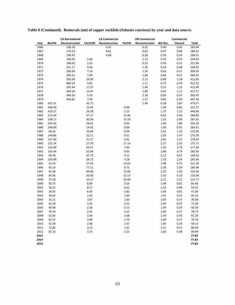
Table 8 (Continued). Removals (mt) of copper rockfish (Sebastes caurinus) by year and data source.





1966 158.18 6.41 0.22 0.40 0.43 165.641967 170.13 8.61 0.62 0.47 0.60 180.421968 190.42 4.66 0.58 0.50 0.34 196.511969 190.05 2.66 1.15 0.53 0.25 194.641970 248.03 2.63 0.53 0.56 0.21 251.961971 231.17 4.66 1.20 0.59 0.38 238.011972 300.04 7.14 1.56 0.63 0.57 309.931973 350.52 7.04 1.68 0.66 0.57 360.451974 392.04 16.00 2.12 0.69 1.18 412.031975 400.14 9.65 1.11 0.72 0.70 412.321976 395.44 17.37 1.49 0.37 1.23 415.901977 399.16 15.47 1.80 0.02 1.12 417.571978 384.26 5.03 2.18 0.50 0.47 392.451979 436.82 7.44 1.57 0.85 0.59 447.261980 432.31 42.71 1.40 0.28 2.87 479.571981 506.40 13.04 0.00 1.28 0.85 521.571982 419.17 16.58 2.13 1.37 1.22 440.461983 213.54 57.17 12.96 0.63 4.56 288.861984 238.17 30.30 14.33 1.32 2.90 287.021985 294.56 28.62 0.05 1.06 1.86 326.161986 248.09 14.02 0.00 1.40 0.91 264.411987 96.26 16.84 0.09 1.61 1.10 115.901988 144.86 22.11 0.51 1.83 1.47 170.781989 137.40 31.57 4.91 2.05 2.37 178.301990 125.74 27.70 17.14 2.27 2.92 175.771991 114.09 50.57 7.63 1.50 3.79 177.581992 102.44 62.96 9.95 2.86 4.74 182.951993 90.78 67.73 4.12 2.12 4.67 169.431994 103.09 34.72 4.28 1.33 2.54 145.961995 41.59 57.04 16.03 1.98 4.75 121.391996 93.14 77.11 8.75 2.39 5.59 186.981997 44.28 69.46 12.06 2.25 5.30 133.361998 46.96 50.90 12.13 2.32 4.10 116.401999 75.58 25.17 10.48 2.21 2.32 115.772000 50.75 8.89 3.54 2.48 0.81 66.462001 36.25 8.17 6.61 2.53 0.96 54.512002 26.05 6.66 5.82 1.66 0.81 41.002003 39.62 1.63 1.84 1.91 0.23 45.232004 31.21 3.87 1.83 2.03 0.37 39.302005 62.28 3.25 2.51 2.95 0.37 71.362006 49.98 2.26 2.12 1.94 0.29 56.592007 70.59 2.61 3.15 2.00 0.37 78.732008 55.83 3.00 3.68 2.34 0.43 65.292009 62.57 3.89 1.79 2.09 0.37 70.702010 52.28 2.68 1.07 1.85 0.24 58.132011 72.85 3.12 1.61 2.51 0.31 80.392012 87.10 3.75 2.15 1.60 0.38 94.992013 77.832014 77.832015 77.83

63

Table 9. Removals (mt) of sharpchin rockfish (Sebastes zacentrus) by year and region.


CentralCalifornia


SouthernCalifornia

CentralCalifornia


1916 0.00 0.02 0.00 0.02 1966 0.00 0.14 891.48 891.621917 0.00 0.03 0.00 0.03 1967 0.00 0.13 510.79 510.921918 0.00 0.03 0.00 0.03 1968 0.00 0.11 298.87 298.991919 0.00 0.02 0.00 0.02 1969 0.00 0.19 32.77 32.971920 0.00 0.02 0.00 0.02 1970 0.00 0.28 46.46 46.741921 0.00 0.02 0.00 0.02 1971 0.00 0.23 67.23 67.461922 0.00 0.02 0.00 0.02 1972 0.00 0.37 44.45 44.821923 0.00 0.02 0.00 0.02 1973 0.00 2.40 68.55 70.951924 0.00 0.01 0.00 0.01 1974 0.00 2.71 40.22 42.931925 0.00 0.01 0.00 0.01 1975 0.00 3.03 43.27 46.301926 0.00 0.03 0.00 0.03 1976 0.00 3.18 33.75 36.931927 0.00 0.04 0.00 0.04 1977 0.00 1.12 11.47 12.591928 0.00 0.06 0.00 0.06 1978 0.00 0.07 179.87 179.941929 0.00 0.06 0.02 0.07 1979 0.00 3.59 184.26 187.851930 0.00 0.06 0.01 0.07 1980 0.00 0.00 176.32 176.321931 0.00 0.02 0.03 0.05 1981 0.00 0.00 27.70 27.701932 0.00 0.03 0.02 0.05 1982 0.00 0.00 25.93 25.931933 0.00 0.04 0.04 0.08 1983 0.00 1.39 494.09 495.481934 0.00 0.05 0.03 0.08 1984 0.00 3.91 171.81 175.721935 0.00 0.05 0.03 0.08 1985 0.00 10.91 624.42 635.331936 0.00 0.06 0.02 0.07 1986 0.00 1.93 432.46 434.391937 0.00 0.05 0.04 0.09 1987 0.00 0.13 418.29 418.421938 0.00 0.06 0.05 0.11 1988 0.00 0.00 867.83 867.831939 0.00 0.06 0.10 0.16 1989 0.00 8.57 913.37 921.931940 0.00 0.08 0.35 0.42 1990 0.00 31.65 672.74 704.401941 0.00 0.13 0.56 0.69 1991 0.00 17.46 438.01 455.471942 0.00 0.04 1.01 1.04 1992 0.09 19.63 379.91 399.621943 0.00 0.06 3.54 3.60 1993 0.05 9.11 743.94 753.101944 0.00 0.08 5.69 5.78 1994 0.00 32.86 797.44 830.301945 0.00 0.14 10.56 10.69 1995 0.00 11.07 439.66 450.731946 0.00 0.32 6.84 7.16 1996 0.00 37.98 388.98 426.961947 0.00 0.15 4.23 4.38 1997 0.00 181.91 462.55 644.461948 0.00 0.24 4.28 4.51 1998 0.00 17.04 182.59 199.631949 0.00 0.13 5.10 5.23 1999 0.00 0.96 92.89 93.851950 0.00 0.17 5.80 5.97 2000 0.00 0.70 17.48 18.181951 0.00 0.36 5.70 6.06 2001 0.00 0.08 13.45 13.531952 0.00 0.38 10.02 10.40 2002 0.00 0.43 9.09 9.521953 0.00 0.33 6.75 7.07 2003 0.00 0.00 8.01 8.011954 0.00 0.22 10.14 10.37 2004 0.00 0.00 38.18 38.181955 0.00 0.15 7.62 7.77 2005 0.00 0.00 5.75 5.751956 0.00 0.33 12.83 13.16 2006 0.00 0.00 0.26 0.261957 0.00 0.32 11.97 12.30 2007 0.00 0.00 3.84 3.841958 0.00 0.31 10.73 11.04 2008 0.00 0.00 1.84 1.841959 0.00 0.28 9.58 9.85 2009 0.00 0.00 2.04 2.041960 0.00 0.26 12.37 12.63 2010 0.00 0.00 0.57 0.571961 0.00 0.14 14.54 14.68 2011 0.00 0.00 0.78 0.781962 0.00 0.15 18.62 18.77 2012 0.00 0.00 13.69 13.691963 0.00 0.18 23.70 23.88 2013 5.011964 0.00 0.10 21.21 21.31 2014 5.011965 0.00 0.10 19.93 20.03 2015 5.01

64

Table 10. Removals (mt) of sharpchin rockfish (Sebastes zacentrus) by year and data source.

YearCA Commercial Reconstruction CALCOM

OR Commercial Reconstruction PacFIN Tagart

Pac. Fisherman and PMFC Data Series NORPAC

Foreign Fisheries


1916 0.01 0.00 0.01 0.021917 0.01 0.00 0.01 0.031918 0.02 0.00 0.02 0.031919 0.01 0.00 0.01 0.021920 0.01 0.00 0.01 0.021921 0.01 0.00 0.01 0.021922 0.01 0.00 0.01 0.021923 0.01 0.00 0.01 0.021924 0.00 0.00 0.01 0.011925 0.00 0.00 0.00 0.011926 0.01 0.00 0.01 0.031927 0.02 0.00 0.02 0.041928 0.03 0.00 0.03 0.061929 0.03 0.00 0.04 0.071930 0.03 0.00 0.04 0.071931 0.02 0.00 0.02 0.051932 0.02 0.00 0.03 0.051933 0.04 0.00 0.04 0.081934 0.04 0.00 0.04 0.081935 0.04 0.00 0.04 0.081936 0.03 0.00 0.04 0.071937 0.04 0.00 0.05 0.091938 0.05 0.00 0.06 0.111939 0.07 0.01 0.08 0.161940 0.08 0.12 0.22 0.421941 0.13 0.19 0.36 0.691942 0.05 0.36 0.09 0.55 1.041943 0.08 1.24 0.38 1.89 3.601944 0.13 2.17 0.44 3.04 5.781945 0.33 3.36 1.38 5.62 10.691946 0.41 2.12 0.86 3.77 7.161947 0.20 1.36 0.52 2.31 4.381948 0.31 0.95 0.88 2.37 4.511949 0.16 1.24 1.08 2.75 5.231950 0.14 1.64 1.05 3.14 5.971951 0.28 1.74 0.85 3.19 6.061952 0.27 3.38 1.29 5.47 10.401953 0.24 2.18 0.93 3.72 7.071954 0.13 3.03 1.76 5.45 10.371955 0.10 2.41 1.18 4.09 7.771956 0.18 3.90 2.16 6.92 13.161957 0.19 3.89 1.75 6.47 12.301958 0.20 3.04 2.00 5.81 11.041959 0.18 2.21 2.28 5.18 9.851960 0.21 3.02 2.75 6.64 12.631961 0.09 3.89 2.98 7.72 14.681962 0.08 4.80 4.01 9.87 18.771963 0.11 8.63 2.58 12.56 23.881964 0.06 7.48 2.57 11.21 21.311965 0.08 7.18 2.24 10.53 20.03

65

Table 10 (Continued). Removals (mt) of sharpchin rockfish (Sebastes zacentrus) by year and data source.



Pac. Fisherman and PMFC Data Series NORPAC

Foreign Fisheries


1966 0.08 14.92 2.70 405.00 468.92 891.621967 0.08 9.13 233.00 268.70 510.921968 0.08 3.66 138.00 157.24 298.991969 0.09 0.14 0.40 15.00 17.34 32.971970 0.13 1.83 4.20 16.00 24.58 46.741971 0.11 11.57 6.30 14.00 35.48 67.461972 0.18 3.17 5.90 12.00 23.57 44.821973 0.14 1.90 0.60 31.00 37.32 70.951974 0.29 4.17 0.90 15.00 22.58 42.931975 0.43 6.51 15.00 24.35 46.301976 0.51 7.10 0.90 9.00 19.42 36.931977 0.53 3.34 2.10 6.62 12.591978 0.03 33.57 51.70 94.63 179.941979 1.70 57.95 29.40 98.79 187.851980 0.00 53.69 29.90 92.73 176.321981 0.00 13.13 14.57 27.701982 0.00 12.29 13.64 25.931983 0.66 234.24 260.58 495.481984 1.85 81.45 92.41 175.721985 5.17 296.02 334.13 635.331986 0.91 205.02 228.45 434.391987 0.06 200.98 217.38 418.421988 0.00 422.67 445.16 867.831989 4.23 451.02 466.68 921.931990 15.85 336.87 0.00 351.68 704.401991 8.87 222.40 0.05 224.15 455.471992 10.16 185.74 10.00 193.72 399.621993 4.79 388.92 0.00 359.38 753.101994 17.43 423.07 0.03 389.76 830.301995 5.96 236.76 0.04 207.97 450.731996 20.77 212.70 0.02 193.47 426.961997 101.03 256.89 0.01 286.53 644.461998 9.62 102.95 0.07 87.00 199.631999 0.55 53.22 0.03 40.05 93.852000 0.41 10.16 0.02 7.59 18.182001 0.05 5.90 2.06 5.52 13.532002 0.26 5.40 0.07 3.78 9.522003 0.00 3.79 1.12 3.10 8.012004 0.00 23.79 0.01 14.38 38.182005 0.00 3.63 0.02 2.10 5.752006 0.00 0.14 0.03 0.09 0.262007 0.00 1.74 0.79 1.31 3.842008 0.00 1.23 0.00 0.61 1.842009 0.00 1.37 0.00 0.67 2.042010 0.00 0.38 0.00 0.19 0.572011 0.00 0.52 0.01 0.26 0.782012 0.00 9.17 0.00 4.51 13.692013 5.012014 5.012015 5.01

66

Table 11. Removals (mt) of stripetail rockfish (Sebastes saxicola) by year and region.


CentralCalifornia


SouthernCalifornia

CentralCalifornia


1916 0.00 7.70 0.15 7.85 1966 0.01 18.40 78.25 96.661917 0.00 12.17 0.29 12.46 1967 0.02 11.68 62.12 73.831918 0.00 12.23 0.58 12.81 1968 0.01 11.59 127.15 138.751919 0.00 8.14 0.13 8.27 1969 0.00 10.67 34.17 44.841920 0.00 8.51 0.18 8.69 1970 0.00 14.99 39.68 54.671921 0.00 7.11 0.27 7.38 1971 0.00 11.45 55.99 67.441922 0.00 6.57 0.22 6.79 1972 0.00 19.83 66.92 86.751923 0.00 8.16 0.08 8.24 1973 0.00 51.02 229.59 280.621924 0.00 8.00 0.38 8.38 1974 0.00 59.49 50.08 109.581925 0.00 8.42 1.09 9.51 1975 0.00 61.65 77.14 138.791926 0.00 11.95 0.85 12.80 1976 0.00 64.88 47.50 112.381927 0.00 9.34 1.43 10.77 1977 0.00 42.91 6.20 49.101928 0.00 9.68 0.87 10.56 1978 0.00 17.39 7.71 25.101929 0.00 6.14 4.25 10.39 1979 0.00 47.21 17.09 64.301930 0.00 8.37 3.39 11.76 1980 0.00 61.54 5.92 67.471931 0.00 6.32 7.27 13.59 1981 0.00 35.49 0.37 35.851932 0.00 4.80 3.95 8.75 1982 0.00 25.36 17.78 43.141933 0.00 3.93 3.35 7.28 1983 0.00 3.60 35.22 38.811934 0.00 4.22 3.10 7.32 1984 0.00 6.85 25.43 32.281935 0.00 4.00 4.34 8.34 1985 0.00 16.25 40.30 56.551936 0.00 4.00 1.67 5.67 1986 0.00 10.95 12.11 23.061937 0.00 3.40 2.11 5.51 1987 0.00 16.75 16.11 32.851938 0.00 3.10 2.49 5.59 1988 0.00 10.90 15.77 26.681939 0.00 2.95 3.85 6.80 1989 0.00 10.73 23.07 33.811940 0.00 2.28 3.47 5.75 1990 0.00 7.22 33.48 40.711941 0.00 2.33 2.93 5.26 1991 0.00 11.07 59.99 71.051942 0.00 0.79 1.27 2.07 1992 0.00 2.40 11.51 13.901943 0.00 0.96 2.38 3.34 1993 0.00 19.33 39.49 58.821944 0.00 2.37 6.26 8.63 1994 0.00 30.63 109.98 140.611945 0.00 3.40 15.81 19.22 1995 0.00 46.78 20.46 67.241946 0.00 6.04 12.52 18.56 1996 0.00 6.78 19.31 26.101947 0.00 3.40 8.83 12.23 1997 0.00 12.79 25.26 38.041948 0.00 3.42 10.33 13.75 1998 0.00 34.01 28.49 62.501949 0.00 7.43 15.83 23.26 1999 0.00 6.40 27.05 33.451950 0.00 11.28 14.96 26.24 2000 0.01 1.27 7.77 9.051951 0.00 20.62 12.46 33.08 2001 0.00 0.54 18.86 19.401952 0.00 18.69 8.69 27.38 2002 0.00 0.32 6.50 6.821953 0.00 20.90 8.09 28.99 2003 0.00 0.05 2.87 2.911954 0.00 17.94 20.77 38.71 2004 0.00 0.14 3.26 3.401955 0.00 9.78 20.23 30.02 2005 0.00 0.31 6.02 6.331956 0.00 15.61 32.70 48.32 2006 0.00 0.00 7.26 7.261957 0.01 13.49 17.85 31.35 2007 0.00 0.00 8.21 8.221958 0.01 21.77 8.07 29.85 2008 0.00 0.00 8.63 8.631959 0.01 21.36 6.67 28.04 2009 0.00 0.00 3.19 3.191960 0.01 13.76 12.22 25.99 2010 0.00 0.00 1.84 1.841961 0.01 12.82 9.78 22.61 2011 0.00 0.00 3.83 3.831962 0.01 13.11 10.04 23.17 2012 0.00 0.29 4.16 4.451963 0.01 13.16 7.87 21.04 2013 3.371964 0.00 10.48 11.15 21.63 2014 3.371965 0.01 10.25 17.79 28.05 2015 3.37

67

Table 12. Removals (mt) of stripetail rockfish (Sebastes saxicola) by year and data source.



Foreign Fisheries


1916 6.42 1.43 7.851917 10.18 2.27 12.461918 10.47 2.34 12.811919 6.76 1.51 8.271920 7.10 1.59 8.691921 6.03 1.35 7.381922 5.55 1.24 6.791923 6.73 1.50 8.241924 6.85 1.53 8.381925 7.78 1.74 9.511926 10.46 2.34 12.801927 8.80 1.97 10.771928 8.63 1.93 10.561929 8.49 1.90 10.391930 9.62 2.15 11.761931 11.11 2.48 13.591932 7.15 1.60 8.751933 5.95 1.33 7.281934 5.99 1.34 7.321935 6.81 1.52 8.341936 4.63 1.03 5.671937 4.51 1.01 5.511938 4.57 1.02 5.591939 5.56 1.24 6.801940 4.70 1.05 5.751941 4.30 0.96 5.261942 1.66 0.03 0.38 2.071943 2.48 0.25 0.61 3.341944 6.63 0.43 1.58 8.631945 15.66 0.05 3.51 19.221946 14.97 0.21 3.39 18.561947 9.38 0.61 2.23 12.231948 8.68 2.56 2.51 13.751949 16.27 2.74 4.25 23.261950 20.01 1.44 4.79 26.241951 24.63 2.41 6.04 33.081952 18.95 3.43 5.00 27.381953 21.85 1.85 5.29 28.991954 21.05 10.60 7.07 38.711955 14.87 9.67 5.48 30.021956 15.94 23.56 8.82 48.321957 13.72 11.90 5.72 31.351958 21.37 3.03 5.45 29.851959 20.10 2.82 5.12 28.041960 13.70 7.54 4.74 25.991961 12.02 6.47 4.13 22.611962 12.17 6.77 4.23 23.171963 13.43 3.77 3.84 21.041964 10.15 7.53 3.95 21.631965 11.94 10.99 5.12 28.05

68

Table 12 (Continued). Removals (mt) of stripetail rockfish (Sebastes saxicola) by year and data source.



Foreign Fisheries


1966 10.41 12.60 56.00 17.65 96.661967 13.32 15.02 32.00 13.48 73.831968 11.64 2.79 99.00 25.33 138.751969 10.28 2.38 24.00 8.19 44.841970 13.85 1.84 29.00 9.98 54.671971 11.96 21.17 22.00 12.31 67.441972 18.28 17.63 35.00 15.84 86.751973 22.04 2.35 205.00 51.23 280.621974 25.48 4.09 60.00 20.00 109.581975 32.82 1.64 79.00 25.34 138.791976 36.74 0.12 55.00 20.51 112.381977 37.78 0.66 1.70 8.96 49.101978 16.15 4.17 0.20 4.58 25.101979 45.34 6.92 0.30 11.74 64.301980 52.66 2.49 12.32 67.471981 29.01 0.30 6.55 35.851982 20.73 14.54 7.88 43.141983 2.94 28.79 7.09 38.811984 5.60 20.79 5.89 32.281985 13.28 32.94 10.32 56.551986 8.95 9.90 4.21 23.061987 13.69 13.17 6.00 32.851988 8.91 12.89 4.87 26.681989 8.77 18.86 6.17 33.811990 5.91 27.37 7.43 40.711991 9.05 49.04 12.97 71.051992 1.96 9.41 2.54 13.901993 15.80 32.28 10.74 58.821994 25.04 89.90 25.67 140.611995 38.24 16.72 12.27 67.241996 5.54 15.79 4.76 26.101997 10.45 20.65 6.95 38.041998 27.80 23.29 11.41 62.501999 5.23 22.11 6.11 33.452000 1.04 6.35 1.65 9.052001 0.44 15.42 3.54 19.402002 0.26 5.31 1.25 6.822003 0.04 2.34 0.53 2.912004 0.11 2.67 0.62 3.402005 0.25 4.92 1.16 6.332006 0.00 5.93 1.32 7.262007 0.00 6.71 1.50 8.222008 0.00 7.06 1.58 8.632009 0.00 2.60 0.58 3.192010 0.00 1.50 0.34 1.842011 0.00 3.13 0.70 3.832012 0.23 3.40 0.81 4.452013 3.372014 3.372015 3.37

69

Table 13. Removals (mt) of yellowtail rockfish (Sebastes flavidus) by year and region. Only removals for northern California, Oregon, and Washington (“No. CA / OR / WA”) were included in the assessment of the northern stock. Catch prior to 1916 (not shown) averaged < 1mt yr-1.


CentralCalifornia


SouthernCalifornia

CentralCalifornia


1916 2.61 526.48 3.04 532.12 1966 5.71 320.66 4896.57 5222.941917 4.21 818.42 5.01 827.64 1967 8.94 317.50 3016.48 3342.931918 3.84 957.57 10.29 971.69 1968 10.06 275.44 3321.47 3606.971919 2.29 663.84 3.31 669.44 1969 37.32 194.61 3821.11 4053.031920 2.49 677.46 4.11 684.07 1970 26.22 226.47 2215.58 2468.271921 2.18 560.26 5.59 568.03 1971 33.18 256.99 1674.71 1964.881922 2.14 482.10 4.56 488.80 1972 47.10 342.40 2533.20 2922.701923 2.87 521.01 2.47 526.35 1973 53.63 564.94 2347.89 2966.461924 3.85 304.79 4.33 312.97 1974 60.06 687.61 1702.74 2450.411925 4.22 391.33 10.79 406.34 1975 54.73 730.51 1428.23 2213.461926 5.24 604.38 10.72 620.34 1976 60.88 519.57 4324.37 4904.821927 4.35 489.66 18.98 512.98 1977 68.31 525.74 5087.00 5681.051928 3.71 575.73 17.71 597.15 1978 69.40 360.81 8282.49 8712.701929 3.76 486.22 26.03 516.00 1979 95.54 430.50 8047.55 8573.591930 3.84 709.40 36.92 750.15 1980 111.20 410.83 7889.59 8411.621931 1.26 646.46 41.93 689.66 1981 104.00 736.43 9298.11 10138.541932 6.54 517.67 27.92 552.13 1982 157.37 1392.66 9799.27 11349.301933 1.02 332.42 25.96 359.39 1983 90.01 1508.64 8931.04 10529.691934 3.47 372.99 22.91 399.37 1984 138.32 1689.13 5521.20 7348.651935 4.00 449.44 34.89 488.33 1985 183.34 895.84 3769.61 4848.791936 4.69 555.50 40.03 600.22 1986 152.17 735.04 5397.86 6285.061937 2.84 503.56 48.18 554.59 1987 15.96 766.93 5268.11 6051.001938 1.61 404.12 55.26 461.00 1988 61.07 391.19 6956.76 7409.021939 1.54 287.25 62.70 351.49 1989 98.27 1095.50 6181.38 7375.151940 1.87 445.36 140.32 587.55 1990 60.75 1031.22 5237.92 6329.881941 2.02 442.14 188.62 632.78 1991 39.27 444.33 5285.16 5768.771942 0.93 145.02 341.40 487.35 1992 37.50 645.38 8376.06 9058.941943 0.73 176.69 1116.69 1294.11 1993 22.84 275.91 7708.45 8007.201944 0.58 205.44 1936.51 2142.53 1994 9.23 278.20 7584.35 7871.781945 1.08 336.43 3390.80 3728.31 1995 24.19 217.57 6857.31 7099.071946 1.27 456.51 2201.01 2658.79 1996 6.10 232.64 8673.57 8912.311947 0.82 361.36 1209.00 1571.18 1997 16.20 734.14 3151.10 3901.441948 1.11 367.02 1076.04 1444.17 1998 9.09 433.12 4214.20 4656.411949 1.29 342.91 951.84 1296.04 1999 10.08 237.82 4816.41 5064.321950 1.79 489.33 961.39 1452.51 2000 0.53 160.75 5011.83 5173.111951 2.37 480.88 855.03 1338.28 2001 0.28 57.43 3387.20 3444.911952 2.34 378.51 1008.62 1389.46 2002 0.12 26.43 2452.14 2478.691953 1.13 196.98 796.00 994.12 2003 0.07 19.47 1490.02 1509.551954 2.01 251.50 1147.37 1400.88 2004 0.67 12.74 1750.19 1763.601955 2.69 265.29 975.55 1243.53 2005 1.76 23.57 966.08 991.401956 3.82 482.76 1475.46 1962.03 2006 1.69 22.49 510.82 535.001957 4.41 495.94 1610.52 2110.88 2007 1.87 57.95 405.36 465.181958 5.10 807.10 1434.98 2247.17 2008 4.21 17.82 511.05 533.081959 11.31 668.10 1588.92 2268.34 2009 0.89 48.24 817.39 866.511960 4.42 388.35 1994.72 2387.48 2010 1.01 23.97 1026.61 1051.581961 5.33 284.58 1963.13 2253.04 2011 0.62 45.29 1456.02 1501.931962 4.26 237.63 2447.96 2689.85 2012 2.42 52.30 1646.36 1701.081963 3.90 203.58 1900.84 2108.32 2013 1376.331964 2.74 138.02 1598.46 1739.22 2014 1376.331965 5.55 199.76 1573.93 1779.25 2015 1376.33

70

Table 14. Removals (mt) of yellowtail rockfish (Sebastes flavidus) north of Cape Mendocino, by year and data source. Catch prior to 1916 (not shown) averaged <1 mt yr-1.

YearOR Commercial Reconstruction PacFIN Tagart

Pac. Fisherman and PMFC Data Wallace and Lai Foreign Fisheries NORPAC CALCOM

CA Commercial Reconstruction

CA Recreational Reconstruction RecFIN WA Recreational


1916 1.00 1.90 0.14 3.041917 1.05 3.74 0.23 5.011918 1.10 8.72 0.47 10.291919 1.15 2.00 0.15 3.311920 1.20 2.72 0.19 4.111921 1.26 4.08 0.25 5.591922 1.31 3.04 0.21 4.561923 1.36 1.00 0.11 2.471924 1.41 2.73 0.20 4.331925 1.46 8.84 0.49 10.791926 1.51 8.72 0.49 10.721927 1.56 16.55 0.86 18.981928 2.61 14.28 0.02 0.80 17.711929 9.13 15.68 0.03 1.18 26.031930 12.48 22.73 0.04 1.67 36.921931 7.14 32.84 0.05 1.90 41.931932 1.81 24.79 0.07 1.26 27.921933 2.88 21.84 0.08 1.17 25.961934 3.12 18.67 0.09 1.03 22.911935 2.03 31.18 0.11 1.58 34.891936 10.08 28.02 0.12 1.81 40.031937 23.00 22.87 0.14 2.18 48.181938 22.93 29.69 0.14 2.50 55.261939 28.53 31.21 0.12 2.84 62.701940 119.04 14.75 0.17 6.35 140.321941 159.22 20.69 0.16 8.55 188.621942 282.71 26.21 16.92 0.09 15.48 341.401943 924.12 113.11 28.74 0.08 50.63 1116.691944 1572.57 130.03 146.04 0.07 87.81 1936.511945 2420.25 407.74 408.98 0.09 153.76 3390.801946 1507.08 255.74 338.25 0.15 99.80 2201.011947 916.75 152.63 84.67 0.12 54.82 1209.001948 627.00 260.00 140.01 0.24 48.78 1076.041949 541.10 319.49 47.79 0.32 43.15 951.841950 581.15 309.35 26.93 0.38 43.58 961.391951 512.86 251.82 51.16 0.44 38.75 855.031952 537.31 380.29 44.92 0.38 45.72 1008.621953 444.58 276.16 38.86 0.33 36.08 796.001954 530.71 519.48 44.77 0.41 52.01 1147.371955 568.14 348.64 14.07 0.48 44.22 975.551956 755.16 639.14 13.74 0.54 66.88 1475.461957 996.71 519.10 21.09 0.62 73.00 1610.521958 751.99 590.51 26.89 0.54 65.05 1434.981959 824.58 673.38 18.48 0.45 72.03 1588.921960 1075.78 814.22 13.99 0.28 90.44 1994.721961 977.46 882.25 9.05 0.23 5.37 88.77 1963.131962 1131.41 1186.28 8.90 0.11 10.74 110.51 2447.961963 960.83 816.53 21.83 0.08 16.12 85.46 1900.841964 687.66 792.17 25.55 0.09 21.49 71.51 1598.461965 675.10 779.10 22.57 0.16 26.86 70.15 1573.93

71

Table 14 (Continued). Removals (mt) of yellowtail rockfish (Sebastes flavidus) north of Cape Mendocino, by year and data source. Catch prior to 1916 (not shown) averaged <1 mt yr-1.

YearOR Commercial Reconstruction PacFIN Tagart

Pac. Fisherman and PMFC Data Wallace and Lai Foreign Fisheries NORPAC CALCOM


CA Recreational Reconstruction RecFIN WA Recreational


1966 818.87 968.40 2845.00 11.45 0.04 32.23 220.58 4896.571967 835.23 34.70 1.40 1956.00 16.31 0.16 37.61 135.07 3016.481968 981.83 951.50 0.00 1187.00 17.63 0.09 34.36 149.05 3321.471969 1378.58 1372.60 21.70 786.00 58.95 0.31 31.12 171.85 3821.111970 521.79 464.80 10.20 1031.00 60.66 0.06 27.87 99.20 2215.581971 674.15 365.10 9.70 434.00 92.23 0.08 24.63 74.82 1674.711972 1113.73 456.90 11.30 716.00 99.77 0.21 21.39 113.89 2533.201973 1071.76 275.90 20.50 770.00 85.82 0.12 18.14 105.64 2347.891974 780.20 50.20 16.90 654.00 109.94 0.07 14.90 76.53 1702.741975 707.49 330.30 5.60 222.00 86.92 0.03 11.65 64.23 1428.231976 1338.84 2363.80 63.70 235.00 111.59 0.04 16.03 195.36 4324.371977 1513.10 2955.50 269.50 111.06 0.06 7.45 230.33 5087.001978 2221.52 5191.00 184.90 297.22 0.47 12.38 375.00 8282.491979 2061.90 5311.80 237.00 67.53 0.53 4.07 364.72 8047.551980 3048.51 4235.50 181.30 37.46 27.54 2.89 356.38 7889.591981 8722.79 141.60 8.65 4.02 421.06 9298.111982 8902.01 434.80 17.24 1.72 443.50 9799.271983 8145.19 363.60 15.32 2.77 404.17 8931.041984 4866.72 369.80 32.51 3.43 248.73 5521.201985 3037.51 358.70 45.80 4.95 322.64 3769.611986 4167.96 740.90 13.59 9.06 466.34 5397.861987 3956.79 830.70 14.59 11.21 454.81 5268.111988 5669.20 663.90 8.64 13.37 601.64 6956.761989 4553.33 1050.00 30.22 15.52 532.32 6181.381990 4195.53 566.60 2.60 2.86 17.68 452.65 5237.921991 3574.14 863.40 354.75 2.26 35.35 455.27 5285.161992 5494.09 1463.00 662.35 1.05 31.73 723.85 8376.061993 5010.89 1612.50 307.32 77.67 41.66 658.42 7708.451994 5174.43 1142.80 566.33 28.87 17.98 653.94 7584.351995 4664.64 781.00 779.28 25.72 15.31 591.37 6857.311996 5159.88 2013.40 710.07 20.63 20.68 748.92 8673.571997 1825.46 583.70 418.53 33.38 21.40 268.63 3151.101998 2467.05 763.90 555.66 36.13 31.73 359.73 4214.201999 2226.47 977.00 1161.80 24.88 11.56 414.70 4816.412000 2830.07 1082.10 636.28 18.12 13.16 432.10 5011.832001 1883.47 976.40 209.82 17.22 8.68 291.62 3387.202002 1017.57 1007.70 193.60 19.27 3.20 210.79 2452.142003 413.54 887.90 35.30 15.80 10.49 126.99 1490.022004 567.58 958.50 43.31 11.69 20.02 149.09 1750.192005 746.50 108.38 12.54 17.45 81.21 966.082006 338.83 108.95 8.79 11.71 42.54 510.822007 274.34 77.21 6.96 13.45 33.40 405.362008 272.77 173.56 5.48 16.85 42.40 511.052009 536.08 177.54 10.26 25.71 67.79 817.392010 748.57 149.75 7.92 35.02 85.34 1026.612011 1181.03 101.11 12.40 39.67 121.80 1456.022012 1433.21 41.32 14.68 17.07 140.08 1646.362013 1376.332014 1376.332015 1376.33

72

Table 15. Removals (mt) of English sole (Parophrys vetulus) by year and region.

YearSouthern & Central

CaliforniaNo. CA /OR / WA

Discard (Coastwide) Total Year

Southern & CentralCalifornia

No. CA /OR / WA

Discard (Coastwide) Total

1876 1.0 0.0 0 1.0 1946 717.1 3544.0 737 4998.11877 1.2 0.0 0 1.2 1947 776.1 2055.9 502 3334.01878 1.4 0.0 0 1.4 1948 1208.5 4008.5 814 6030.91879 1.7 0.0 0 1.7 1949 1092.5 1977.5 476 3546.01880 2.1 0.0 0 2.1 1950 1606.8 3311.3 755 5673.11881 2.5 0.0 0 2.5 1951 947.1 2558.2 684 4189.41882 3.0 0.0 0 3.0 1952 736.1 2324.9 763 3824.01883 3.6 0.0 1 4.6 1953 680.8 1589.8 640 2910.61884 4.3 0.0 1 5.3 1954 750.4 1321.1 552 2623.51885 5.2 0.0 1 6.2 1955 837.2 1438.8 553 2829.01886 6.2 0.0 1 7.2 1956 1285.0 1783.0 719 3787.01887 7.4 0.0 1 8.4 1957 1390.0 2190.0 856 4436.01888 8.9 0.0 1 9.9 1958 1132.0 3225.0 1163 5520.01889 10.7 0.0 2 12.7 1959 808.0 3350.0 1269 5427.01890 12.8 0.0 2 14.8 1960 594.0 2829.0 915 4338.01891 15.4 0.0 2 17.4 1961 1082.0 2301.0 805 4188.01892 18.5 0.0 3 21.5 1962 1436.0 2185.0 875 4496.01893 22.2 0.0 3 25.2 1963 1367.0 2230.0 892 4489.01894 26.6 0.0 4 30.6 1964 1453.0 2085.0 1204 4742.01895 31.9 0.0 5 36.9 1965 1696.0 2187.0 1160 5043.01896 38.3 0.0 5 43.3 1966 1470.0 3068.0 984 5522.01897 46.0 0.0 7 53.0 1967 1540.0 2786.0 866 5192.01898 55.2 0.0 8 63.2 1968 1339.0 3200.0 929 5468.01899 66.2 0.0 9 75.2 1969 1012.0 2049.0 727 3788.01900 79.5 0.0 11 90.5 1970 902.0 1593.0 607 3102.01901 95.4 0.0 14 109.4 1971 909.0 1383.0 559 2851.01902 114.5 0.0 16 130.5 1972 793.0 1850.0 657 3300.01903 137.4 0.0 20 157.4 1973 836.0 2134.0 803 3773.01904 164.8 0.0 24 188.8 1974 1012.0 1934.0 912 3858.01905 197.8 0.0 28 225.8 1975 1227.0 2267.0 1085 4579.01906 237.4 0.0 34 271.4 1976 1143.0 3323.0 1289 5755.01907 284.9 0.0 41 325.9 1977 927.0 1940.0 868 3735.01908 341.8 0.0 49 390.8 1978 1070.0 2393.0 1048 4511.01909 410.2 0.0 59 469.2 1979 1115.0 2516.0 1079 4710.01910 492.2 0.0 72 564.2 1980 1362.0 1851.0 930 4143.01911 590.7 0.0 86 676.7 1981 1135.0 1578.8 1155 3868.81912 708.8 0.0 104 812.8 1982 1006.1 1786.5 1171 3963.61913 850.6 0.0 126 976.6 1983 640.8 1714.6 973 3328.41914 1020.7 0.0 152 1172.7 1984 529.6 1191.7 832 2553.31915 1224.8 0.0 184 1408.8 1985 693.9 1236.0 1064 2993.91916 2454.1 0.0 372 2826.1 1986 755.5 1279.8 1138 3173.31917 3343.1 0.0 522 3865.1 1987 746.9 1721.1 1536 4004.01918 2691.7 0.0 440 3131.7 1988 704.4 1396.2 1367 3467.61919 2117.6 0.0 357 2474.6 1989 768.3 1643.9 1390 3802.21920 1463.8 0.0 251 1714.8 1990 712.5 1198.9 1015 2926.41921 1865.6 0.0 318 2183.6 1991 691.7 1492.4 1170 3354.11922 2697.7 0.0 461 3158.7 1992 487.2 1134.7 952 2573.91923 2714.1 0.0 472 3186.1 1993 395.1 1205.4 980 2580.41924 3491.0 0.0 619 4110.0 1994 370.8 751.2 718 1840.01925 3393.3 0.0 625 4018.3 1995 414.6 711.9 646 1772.41926 3246.5 0.0 618 3864.5 1996 436.9 717.6 421 1575.51927 3923.2 0.0 767 4690.2 1997 468.6 1037.9 505 2011.51928 3442.0 0.0 701 4143.0 1998 228.6 909.7 420 1558.31929 3975.7 2.6 832 4810.3 1999 227.3 684.8 392 1304.11930 3065.2 0.8 666 3732.0 2000 181.5 579.1 327 1087.71931 1579.8 0.9 347 1927.7 2001 199.1 790.8 421 1410.91932 2919.2 5.8 615 3540.1 2002 101.7 1066.0 529 1696.61933 2762.1 4.0 580 3346.0 2003 116.8 677.4 338 1132.11934 2350.1 2.4 493 2845.5 2004 98.9 852.7 302 1253.61935 2666.8 5.2 554 3226.0 2005 69.4 854.9 227 1151.41936 2801.0 18.3 585 3404.3 2006 58.0 849.2 192 1099.21937 2547.4 69.3 543 3159.7 2007 63.2 613.6 112.6 789.41938 1076.2 1070.3 397 2543.6 2008 70.5 289.7 59.9 420.11939 1350.6 1176.2 464 2990.8 2009 39.3 317.0 59.3 415.51940 1168.9 1404.8 464 3037.8 2010 21.6 199.7 36.8 258.11941 807.9 1053.6 340 2201.5 2011 17.8 152.1 28.3 198.11942 162.9 1600.1 301 2064.0 2012 18.4 166.8 30.8 216.11943 381.6 2697.1 559 3637.7 2013 224.11944 429.1 1350.4 362 2141.5 2014 224.11945 411.6 1170.4 305 1887.0 2015 224.1

73

Table 16. Removals (mt) of English sole (Parophrys vetulus) by year and data source.

Year Stewart CALCOM PacFIN Discard Total1876 1 0 11877 1 0 11878 1 0 11879 2 0 21880 2 0 21881 2 0 21882 3 0 31883 4 1 51884 4 1 51885 5 1 61886 6 1 71887 7 1 81888 9 1 101889 11 2 131890 13 2 151891 15 2 171892 18 3 211893 22 3 251894 27 4 311895 32 5 371896 38 5 431897 46 7 531898 55 8 631899 66 9 751900 79 11 901901 95 14 1091902 114 16 1301903 137 20 1571904 165 24 1891905 198 28 2261906 237 34 2711907 285 41 3261908 342 49 3911909 410 59 4691910 492 72 5641911 591 86 6771912 709 104 8131913 851 126 9771914 1021 152 11731915 1225 184 14091916 2454 372 28261917 3343 522 38651918 2692 440 31321919 2118 357 24751920 1464 251 17151921 1866 318 21841922 2698 461 31591923 2714 472 31861924 3491 619 41101925 3393 625 40181926 3247 618 3865

1927 3923 767 46901928 3442 701 41431929 3979 832 48111930 3066 666 37321931 1581 347 19281932 2925 615 35401933 2766 580 33461934 2352 493 28451935 2672 554 32261936 2819 585 34041937 2616 543 31591938 2146 397 25431939 2527 464 29911940 2574 464 30381941 1862 340 22021942 1763 301 20641943 3079 559 36381944 1779 362 21411945 1582 305 1887

74

Table 16 (Continued). Removals (mt) of English sole (Parophrys vetulus) by year and data source.

Year Stewart CALCOM PacFIN Discard Total1946 4261 737 49981947 2832 502 33341948 5216 814 60301949 3070 476 35461950 4918 755 56731951 3505 684 41891952 3061 763 38241953 2271 640 29111954 2071 552 26231955 2276 553 28291956 3068 719 37871957 3580 856 44361958 4357 1163 55201959 4158 1269 54271960 3423 915 43381961 3383 805 41881962 3621 875 44961963 3597 892 44891964 3538 1204 47421965 3883 1160 50431966 4538 984 55221967 4326 866 51921968 4539 929 54681969 3061 727 37881970 2495 607 31021971 2292 559 28511972 2643 657 33001973 2970 803 37731974 2946 912 38581975 3494 1085 45791976 4466 1289 57551977 2867 868 37351978 3463 1048 45111979 3631 1079 47101980 3213 930 41431981 2625 1155 37801982 2662 1171 38331983 2118 973 30911984 1626 832 24581985 1891 1064 29551986 2015 1138 31531987 2443 1536 39791988 2055 1367 34221989 2390 1390 37801990 1892 1015 29071991 2169 1170 33391992 1604 952 25561993 1554 980 25341994 1100 718 18181995 1116 646 17621996 1119 421 15401997 1406 505 19111998 1021 420 14411999 853 392 12452000 734 327 10612001 942 421 13632002 1154 529 16832003 787 338 11252004 916 302 12182005 888 227 11152006 886 192 10782007 63.2 613.6 112.6 789.42008 70.5 289.7 59.9 420.12009 39.3 317.0 59.3 415.52010 21.6 199.7 36.8 258.12011 17.8 152.1 28.3 198.12012 18.4 166.8 30.8 216.12013 224.12014 224.12015 224.1

75

Table 17. Removals (mt) of rex sole (Glyptocephalus zachirus) by year and region.


CentralCalifornia


SouthernCalifornia

CentralCalifornia


1916 0.00 131.45 90.86 222.31 1966 21.08 588.54 1637.70 2247.331917 0.00 179.08 123.77 302.85 1967 22.41 703.79 1513.90 2240.101918 0.00 144.19 99.66 243.84 1968 23.33 645.20 1422.42 2090.951919 0.00 113.43 78.40 191.83 1969 29.34 320.55 2072.48 2422.361920 0.00 78.41 54.19 132.60 1970 16.69 373.42 1562.92 1953.041921 0.00 99.93 69.07 169.00 1971 18.65 345.80 1218.26 1582.711922 0.00 144.51 99.88 244.38 1972 29.06 308.54 1636.56 1974.161923 0.00 145.38 100.48 245.86 1973 20.25 266.84 1641.36 1928.451924 0.00 181.27 125.29 306.56 1974 22.40 277.29 1622.48 1922.171925 0.00 179.78 124.26 304.03 1975 10.50 428.07 1450.87 1889.441926 0.00 177.47 122.66 300.12 1976 12.92 624.60 1488.09 2125.621927 0.00 215.01 148.61 363.62 1977 8.98 403.16 1352.12 1764.261928 0.00 210.95 145.80 356.74 1978 4.05 424.78 1661.76 2090.591929 0.00 240.18 166.01 406.19 1979 3.95 452.43 2216.61 2672.991930 0.00 224.13 154.91 379.03 1980 0.23 513.05 1561.37 2074.651931 0.00 283.97 281.60 565.57 1981 1.54 398.30 1633.42 2033.251932 0.00 226.61 152.10 378.71 1982 1.54 454.64 1830.82 2287.011933 0.11 260.30 100.15 360.56 1983 5.63 459.79 1432.62 1898.051934 0.09 348.32 107.13 455.53 1984 2.62 348.62 1302.66 1653.901935 0.39 378.08 51.64 430.11 1985 0.85 652.62 1184.64 1838.111936 0.00 276.59 75.64 352.23 1986 1.59 624.91 915.48 1541.981937 0.00 172.33 141.90 314.23 1987 3.82 607.61 914.82 1526.251938 0.00 231.46 149.36 380.82 1988 2.82 681.69 917.16 1601.681939 0.00 290.59 185.44 476.03 1989 4.58 676.53 759.91 1441.021940 0.00 248.57 194.45 443.02 1990 0.15 489.60 620.98 1110.731941 0.01 155.78 143.62 299.41 1991 0.00 582.36 864.99 1447.341942 0.00 77.57 197.46 275.03 1992 0.18 400.32 678.30 1078.801943 0.00 124.05 591.14 715.18 1993 0.05 392.92 566.49 959.461944 0.00 96.86 284.72 381.58 1994 0.22 524.65 494.32 1019.191945 0.67 142.75 205.74 349.17 1995 2.29 601.75 507.77 1111.801946 0.00 176.25 256.13 432.39 1996 0.60 434.16 579.91 1014.671947 0.10 253.17 366.40 619.67 1997 0.57 356.21 605.99 962.781948 9.64 283.65 558.88 852.17 1998 0.83 196.45 549.39 746.671949 17.34 410.01 540.14 967.48 1999 0.20 178.81 508.06 687.061950 0.53 483.65 438.70 922.87 2000 0.10 148.60 478.03 626.731951 0.85 521.94 450.55 973.34 2001 0.42 114.25 546.84 661.501952 2.54 573.45 555.26 1131.25 2002 0.64 132.72 554.42 687.791953 1.29 431.09 996.85 1429.24 2003 0.07 162.97 512.09 675.131954 5.48 552.48 950.04 1507.99 2004 0.14 150.53 460.84 611.501955 0.47 483.67 1495.40 1979.55 2005 0.02 133.26 528.30 661.581956 2.75 548.00 1809.25 2360.00 2006 0.03 77.04 545.22 622.291957 6.25 523.54 1607.61 2137.40 2007 0.03 56.37 566.65 623.051958 8.91 615.08 1562.20 2186.19 2008 0.06 49.51 545.03 594.601959 9.22 578.99 1444.78 2032.99 2009 0.02 39.14 570.17 609.321960 9.70 472.55 1444.77 1927.01 2010 0.17 21.26 493.33 514.771961 34.43 480.55 1486.90 2001.88 2011 0.97 18.49 407.45 426.911962 47.78 577.44 1658.37 2283.60 2012 0.33 12.68 409.44 422.451963 52.45 659.58 1778.72 2490.74 2013 454.711964 14.92 588.77 1262.33 1866.01 2014 454.711965 30.22 623.29 1147.70 1801.20 2015 454.71

76

Table 18. Removals (mt) of rex sole (Glyptocephalus zachirus) by year and data source.

YearOR Commercial Reconstruction PacFIN CALCOM


CDFG Fish Bulletin No. 74

PMFC Data Series NORPAC


1916 148.2 74.1 222.31917 201.9 100.9 302.81918 162.6 81.3 243.81919 127.9 63.9 191.81920 88.4 44.2 132.61921 112.7 56.3 169.01922 162.9 81.5 244.41923 163.9 82.0 245.91924 204.4 102.2 306.61925 202.7 101.3 304.01926 200.1 100.0 300.11927 242.4 121.2 363.61928 237.8 118.9 356.71929 270.8 135.4 406.21930 252.7 126.3 379.01931 377.0 188.5 565.61932 0.5 252.0 126.2 378.71933 0.2 240.2 120.2 360.61934 0.1 303.6 151.8 455.51935 0.2 286.5 143.4 430.11936 0.9 233.9 117.4 352.21937 4.7 204.8 104.7 314.21938 0.1 253.8 126.9 380.81939 14.6 302.8 158.7 476.01940 26.2 269.1 147.7 443.01941 31.3 168.3 99.8 299.41942 7.6 175.8 91.7 275.01943 252.0 224.8 238.4 715.21944 66.9 187.5 127.2 381.61945 32.2 200.6 116.4 349.21946 29.5 258.7 144.1 432.41947 30.7 382.4 206.6 619.71948 164.9 403.2 284.1 852.21949 206.8 438.2 322.5 967.51950 151.1 464.1 307.6 922.91951 197.5 454.0 321.8 973.31952 228.8 531.5 370.9 1131.21953 508.0 456.7 464.6 1429.21954 507.2 514.8 486.0 1508.01955 862.2 485.0 632.4 1979.61956 804.3 514.9 293.6 747.2 2360.01957 730.4 556.9 179.5 670.6 2137.41958 874.5 626.7 5.5 679.6 2186.21959 666.5 632.7 107.8 626.0 2033.01960 720.1 489.3 130.0 587.7 1927.01961 745.4 526.8 125.1 604.6 2001.91962 918.5 626.4 55.9 682.8 2283.61963 1028.3 696.6 28.6 737.2 2490.71964 687.0 632.4 0.0 546.6 1866.01965 514.7 671.3 93.2 522.1 1801.2

77

Table 18 (Continued). Removals (mt) of rex sole (Glyptocephalus zachirus) by year and data source.

YearOR Commercial Reconstruction PacFIN CALCOM


CDFG Fish Bulletin No. 74

PMFC Data Series NORPAC


1966 873.1 729.7 0.0 644.5 2247.31967 810.7 794.0 0.0 635.4 2240.11968 642.7 861.7 0.0 586.5 2090.91969 726.0 1024.6 0.0 671.8 2422.41970 621.7 789.9 6.1 535.3 1953.01971 510.1 643.9 0.0 428.7 1582.71972 649.6 753.7 42.6 528.3 1974.21973 615.1 718.8 84.8 509.7 1928.51974 621.6 626.7 172.2 501.6 1922.21975 494.5 746.8 161.4 486.7 1889.41976 512.3 913.0 160.0 540.4 2125.61977 452.2 702.2 167.4 442.5 1764.31978 653.8 697.6 222.1 517.1 2090.61979 746.5 868.5 406.1 651.9 2673.01980 541.4 861.6 173.0 498.7 2074.71981 1246.6 305.2 481.5 2033.31982 1403.8 349.8 533.4 2287.01983 1103.7 358.6 435.8 1898.01984 1008.3 271.9 373.7 1653.91985 921.3 508.2 408.6 1838.11986 715.4 489.6 337.0 1542.01987 719.8 481.1 325.4 1526.21988 726.7 542.3 332.7 1601.71989 606.3 543.4 291.3 1441.01990 486.9 393.5 12.0 218.3 1110.71991 699.9 471.2 0.0 276.3 1447.31992 551.3 326.4 1.4 199.7 1078.81993 464.9 322.5 0.0 172.0 959.51994 408.4 433.9 0.3 176.6 1019.21995 422.5 503.0 0.4 186.0 1111.81996 486.4 364.7 0.0 163.5 1014.71997 512.1 301.5 0.0 149.2 962.81998 467.5 168.0 0.2 111.0 746.71999 435.8 153.5 0.0 97.7 687.12000 409.3 128.5 3.8 85.1 626.72001 461.8 99.9 14.4 85.5 661.52002 477.8 117.0 8.7 84.2 687.82003 452.0 144.2 0.8 78.1 675.12004 410.4 134.3 0.3 66.5 611.52005 472.4 119.7 2.2 67.3 661.62006 493.3 69.8 0.3 58.9 622.32007 516.9 51.5 0.2 54.5 623.02008 501.1 45.6 0.3 47.6 594.62009 524.1 36.0 0.4 48.8 609.32010 443.4 19.7 10.4 41.2 514.82011 371.1 17.9 3.8 34.2 426.92012 373.9 12.0 2.8 33.8 422.42013 454.712014 454.712015 454.71

78

7.1.3 Surveys Table 19. Sources of abundance information by species, region and time. Information for vermilion and yellowtail rockfish are included for future assessment efforts.

Spec

ies

Brow

n Ro

ckfis

h

Chin

a Ro

ckfis

h

Copp

er R

ockf

ish

Copp

er R

ockf

ish

Copp

er R

ockf

ish

Engl

ish S

ole

Rex

Sole

Shar

pchi

n Ro

ckfis

h

Strip

etai

l Roc

kfish

Verm

ilion

Rock

fish

Verm

ilion

Rock

fish

Yello

wta

il Roc

kfish

Yello

wta

il Roc

kfish

Species Abbreviation BRWN CHNA COPP COPP COPP EGLS REX SHRP STRK VERM VERM YTRK YTRKArea CEN-NO SOUTH CEN-NO ALL CEN-NO CEN-NO CEN-NO CEN-NO SOUTH CEN CEN NORTHSource Model SurveyTrawl Surveys GLMM Triennial early 80-92 80-92 80-92 80-92 80-92

Triennial late 95-04 95-04 95-04 95-04 95-04NWFSC 03-12 03-12 03-12 03-12 03-12

GLM-stratified Triennial 77-04 77-04 77-04 77-04 77-04 77-04NWFSC 03-12

Hook and Line Survey H&L 04-12Recreational CPUE

RecFIN 80-03 80-03 80-03 80-03 80-03 80-03 80-03 80-03 80-03CenCalOBS 88-?? 88-?? 88-?? 88-?? 88-??

SoCalOBS 99-11 99-11 99-11NoCalOROBS 01-12 01-12 01-12 01-12 01-12 01-12

79

Table 20. Number of tows in the Triennial Survey by year and latitude. Columns: southern boundaries of 2-degree bins.

Table 21. Number of tows in the Triennial Survey by year and depth. Columns: shallow boundaries.

Table 22. Temporal distribution of Triennial Surveys. The three time period groups are used in the stratified GLM analyses. Columns: first day of 10-day Julian date bins.

Latitude: L34 L36 L38 L40 L42 L44 L46 Total1977 109 51 100 20 47 118 126 5711980 23 26 19 71 61 101 3011983 30 36 30 108 99 176 4791986 29 41 25 46 79 263 4831989 30 69 47 33 41 107 113 4401992 18 55 44 36 48 113 107 4211995 43 49 60 43 56 102 84 4371998 46 54 62 50 64 103 89 4682001 47 53 62 47 66 103 86 4642004 22 42 44 44 57 83 76 368Total 315 455 522 347 604 968 1221 4432

CA/OR OR/WAPt. Conception Cape Mendocino Canada

Depth(m): D50 D95 D125 D150 D200 D250 D300 D350 D400 D450 Total1977 101 59 74 89 48 80 44 68 8 5711980 83 54 45 62 29 15 12 1 3011983 121 107 68 72 59 29 18 5 4791986 114 144 89 91 22 10 12 1 4831989 120 104 72 79 29 18 15 3 4401992 114 114 69 60 34 13 16 1 4211995 87 80 54 50 47 17 19 36 28 19 4371998 96 92 57 50 46 18 22 28 35 24 4682001 91 95 54 46 47 17 24 27 40 23 4642004 78 61 47 45 35 22 16 12 38 14 368Total 904 952 614 629 437 207 234 158 209 88 4432

TIMEP:Date: 150 160 170 180 190 200 210 220 230 240 250 260 Total1977 26 83 44 124 34 36 96 73 55 5711980 50 19 56 47 55 45 29 3011983 2 54 86 64 71 98 45 22 37 4791986 32 55 67 98 98 52 62 19 4831989 22 70 73 88 92 95 4401992 15 36 37 40 53 145 74 21 4211995 10 42 63 80 68 106 37 31 4371998 28 99 91 90 94 49 17 4682001 26 90 49 41 58 97 75 28 4642004 78 57 71 74 49 39 368Total 142 288 274 313 525 601 550 437 432 478 260 132 4432

EARLY COMMON LATE

80

Table 23. The total frequency of occurrence by survey and year of each species considered in the category 2 stock assessments.

A) AFSC triennial shelf Group Species 1977 1980 1983 1986 1989 1992 1995 1998 2001 2004 Rockfishes Brown 0% 1% 1% 2% 2% 1% 1% 0% 0% 1% China 0% 0% 0% 0% 0% 0% 0% 0% 0% 0% Copper 0% 0% 1% 0% 3% 1% 1% 1% 1% 0% Sharpchin 13% 15% 19% 20% 19% 16% 11% 11% 10% 14% Stripetail 29% 21% 20% 19% 33% 19% 36% 26% 24% 31% Yellowtail 17% 26% 36% 32% 13% 15% 13% 21% 10% 14% Flatfishes English sole 28% 55% 65% 75% 67% 63% 58% 69% 62% 67% Rex sole 89% 90% 93% 102% 98% 83% 95% 96% 97% 97% B) AFSC triennial slope Group Species 1997 1999 2000 2001 Rockfishes Brown 0% 0% 0% 0% China 0% 0% 0% 0% Copper 0% 0% 0% 0% Sharpchin 12% 11% 8% 9% Stripetail 11% 10% 9% 10% Yellowtail 1% 2% 0% 0% Flatfishes English sole 12% 14% 11% 9% Rex sole 42% 40% 40% 38% C) NWFSC annual shelf-slope Group Species 2003 2004 2005 2006 2007 2008 2009 2010 2011 2012 Rockfishes Brown 1% 1% 1% 1% 0% 0% 0% 0% 1% 1% China 0% 0% 0% 0% 0% 0% 0% 0% 0% 0% Copper 1% 1% 1% 0% 1% 2% 1% 1% 1% 3% Sharpchin 21% 25% 22% 21% 20% 18% 22% 23% 23% 21% Stripetail 10% 7% 5% 7% 5% 4% 6% 6% 7% 6% Yellowtail 6% 6% 7% 6% 7% 5% 6% 7% 7% 7% Flatfishes English sole 41% 46% 45% 36% 35% 35% 36% 40% 43% 43%

Rex sole 65% 66% 67% 62% 62% 59% 58% 62% 62% 62%

81

Table 24. Deviance values for each of the two error structures explored for each stock and survey. Bold values are models with lowest deviance.

Model Survey Species Gamma Lognormal Triennial- early Sharpchin rockfish 5124 4277 Stripetail rockfish 4998 4715

Yellowtail rockfish

(N) 6765 5642 English sole 12176 11366 Rex sole 14725 13757 Triennial- late Sharpchin rockfish 2288 2144 Stripetail rockfish 5063 4861

Yellowtail rockfish

(N) 3119 3002 English sole 9626 9678 Rex sole 14206 14449 Triennial combined

Yellowtail rockfish (N) NA 9683

NWFSC combo Sharpchin rockfish 9585 9248 Stripetail rockfish 4126 4004

Yellowtail rockfish

(N) 4825 4701 English sole 20857 20807 Rex sole 29396 29776

82

Table 25. Final design and model (GLMM)-based survey abundance indices for each survey and stock. Yellowtail rockfish (N) treat the triennial survey as one time series.

Survey Year Design GLMMmed CV Design GLMMmed CV Design GLMMmed CV Design GLMMmed CV Design GLMMmed CVTriennial- Early 1980 4700 15612 0.49 24852 33906 0.45 10590 8962 0.33 4203 4621 0.18 6580 6375 0.18

1983 16192 15974 0.39 7889 9707 0.36 18309 13131 0.19 8369 9250 0.14 13755 13553 0.131986 7499 9735 0.46 7100 17386 0.52 15848 9855 0.28 9543 10549 0.13 15373 16412 0.241989 4688 10330 0.41 10551 14952 0.35 22500 6540 0.29 11949 11490 0.11 16093 16747 0.111992 16428 11786 0.41 7743 13746 0.43 10835 8630 0.27 10550 10292 0.12 14559 16081 0.10

Triennial- Late 1995 5056 5279 0.44 24285 26132 0.32 2713 2924 0.30 10225 11072 0.11 18373 18876 0.081998 3714 3778 0.47 10372 11471 0.35 25545 21151 0.31 15211 14939 0.09 27979 30002 0.092001 5716 3236 0.47 13550 14829 0.34 4414 5022 0.32 16414 17186 0.10 33135 34071 0.082004 2935 6079 0.44 23448 25580 0.33 15232 17350 0.85 37733 34862 0.10 58815 61111 0.09

NWFSC 2003 19398 27362 0.39 164031 105706 0.48 26478 21205 0.47 38697 40260 0.14 56948 58250 0.092004 28373 57970 0.62 21541 20414 0.51 16232 19239 0.55 46476 40948 0.13 54930 57759 0.122005 28254 33980 0.38 21791 13061 0.50 21392 23343 0.43 33160 31870 0.12 51253 52654 0.092006 13559 25856 0.43 5497 15287 0.96 9653 9036 0.47 20985 19478 0.13 48839 50359 0.102007 14136 20347 0.44 2435 10176 0.59 25042 16089 0.44 17803 17713 0.13 45310 49885 0.102008 20765 31124 0.43 3652 33992 0.93 12476 14247 0.47 14895 15061 0.12 35155 37580 0.092009 18634 35855 0.31 7813 3452 0.62 9051 7320 0.47 16484 17286 0.13 35353 36509 0.102010 8639 22998 0.32 782 3540 0.51 28723 37589 0.42 18387 18451 0.13 38564 40698 0.092011 15304 40690 0.33 33482 17191 0.49 30516 25480 0.42 18554 20842 0.12 41530 44484 0.092012 18722 27937 0.39 20594 18651 0.55 38715 14678 0.44 21296 20399 0.13 44622 47233 0.11

SpeciesSharpchin rockfish Stripetail rockfish Yellowtail rockfish (N) English sole Rex sole

83

Table 26. Number of heat treatment samples by power station, over time. Plant acronyms are OBGS = Ormond Beach (Ventura), ESGS = El Segundo, RBGS = Redondo Beach, HBGS = Huntington Beach, SONGS = San Onofre Nuclear (San Clemente).

year ESGS HBGS OBGS RBGS SONGS ALL 1972 17 14 7 38 1973 14 13 8 35 1974 19 13 3 8 43 1975 21 12 4 5 42 1976 20 9 8 18 6 61 1977 21 10 9 3 7 50 1978 12 11 1 8 7 39 1979 16 10 11 12 6 55 1980 13 10 10 12 2 47 1981 14 11 9 10 4 48 1982 15 7 6 13 2 43 1983 10 7 6 12 9 44 1984 6 7 5 10 11 39 1985 12 7 6 13 15 53 1986 9 8 6 17 14 54 1987 9 5 7 9 18 48 1988 6 7 6 8 18 45 1989 3 6 7 7 18 41 1990 7 6 8 9 17 47 1991 5 3 6 8 22 44 1992 9 5 12 9 25 60 1993 5 8 6 10 18 47 1994 8 8 8 11 17 52 1995 5 6 5 8 15 39 1996 5 8 8 12 21 54 1997 9 7 5 12 13 46 1998 3 4 5 8 24 44 1999 3 7 2 19 31 2000 11 1 6 5 20 43 2001 4 3 7 20 18 52 2002 5 7 5 6 22 45 2003 4 7 4 2 20 37 2004 3 7 2 4 18 34 2005 2 4 1 4 24 35 2006 4 5 2 15 26 2007 3 5 1 25 34 2008 3 7 1 22 33 2009 2 3 22 27 2010 2 8 18 28 2011 5 1 25 31

84

Table 27. Number of samples positive for five of the most frequently occurring rockfish species. year bocaccio brown grass olive vermilion

1972 23 8 13 20 1973 17 6 25 12 1974 18 14 20 26 1975 27 35 18 33 1976 12 31 19 26 1977 17 32 18 29 1978 18 17 21 20 1979 18 34 17 32 1980 12 32 19 20 1981 5 22 17 5 1982 3 21 13 2 1983 24 15 2 1984 4 11 8 2 1985 7 30 17 6 1986 5 20 8 9 1987 13 15 8 1988 16 12 11 5 1989 7 15 16 8 1990 3 11 11 3 1991 13 17 17 2 1992 6 23 7 9 1993 1 12 8 2 1994 14 10 4 1995 4 8 2 1 1 1996 4 13 4 1 1997 2 6 1 1998 4 2 1 1999 10 5 1 1 8 2000 7 14 4 3 5 2001 2 11 4 2 2002 8 9 4 1 2 2003 12 17 3 4 5 2004 4 12 4 3 2 2005 13 14 6 2 2006 13 4 4 2007 5 13 4 7 2008 5 13 4 8 2009 8 14 6 8 2010 14 8 9 1 5 2011 3 12 7 1 4

85

Table 28. Sample sizes (trips) by YEAR, COUNTY and REGION from the RecFIN Type 3 database. The shaded cells (Central, 1997-98) are unreliable and are not used.

SOUTH CENTRAL NORTHCO

UN

TY:

SAN

DIE

GO

ORA

NGE

LOS

ANGE

LES

VEN

TURA

SAN

TA B

ARBA

RA

SAN

LU

IS O

BISP

O

MO

NTE

REY

SAN

TA C

RUZ

SAN

MAT

EO

SAN

FRA

NCI

SCO

ALAM

EDA

CON

TRA

COST

A

MAR

IN

SON

OM

A

MEN

DOCI

NO

HUM

BOLD

T

DEL

NO

RTE

CURR

Y

COO

S

DOU

GLAS

LAN

E

LIN

COLN

TILL

AMO

OK

CLAT

SOP

YEAR/FIPS 73 59 37 111 83 79 53 87 81 75 1 13 41 97 45 23 15 15 11 19 39 41 57 7 Total1980 40 70 36 130 85 21 75 1 11 6 6 17 3 3 47 5 5561981 78 144 65 98 85 10 23 2 13 3 1 8 13 7 1 2 37 1 5911982 242 284 157 65 57 6 30 5 12 1 4 7 21 1 2 1 44 2 9411983 276 219 257 83 57 7 39 12 9 3 4 15 4 32 6 10231984 173 207 254 103 28 32 103 41 7 6 7 7 12 4 19 8 32 19 2 10641985 198 170 156 74 26 57 152 43 35 11 4 5 21 19 2 6 17 4 32 13 10451986 83 156 197 80 25 58 85 34 16 8 6 11 10 5 14 4 1 25 11 8291987 22 44 63 5 9 16 15 20 15 9 10 26 5 1 1 4 4 40 5 3141988 22 33 85 79 16 28 28 6 25 2 12 9 27 1 1 2 4 5 5 66 9 4651989 20 16 80 20 10 4 7 21 2 5 3 4 1 2 10 69 274

1993 50 126 219 37 33 14 10 16 2 100 7 1 6151994 136 47 113 46 9 20 16 16 1 1 70 15 4901995 31 19 32 19 7 17 10 5 8 5 5 6 5 1 17 25 72 7 2911996 33 37 40 30 5 42 38 12 27 8 5 22 6 8 2 9 13 70 9 4161997 28 19 32 15 1 58 34 15 23 12 6 45 1 20 19 82 17 4271998 61 30 60 28 9 52 32 20 25 5 25 39 65 6 2 11 20 1 88 26 6051999 56 35 81 36 7 24 27 19 42 2 23 11 23 5 2 14 17 99 24 1 5482000 43 31 77 18 5 13 6 12 14 1 7 12 10 3 8 4 53 21 3382001 35 28 59 21 6 8 10 14 27 7 7 10 5 7 10 1 5 8 47 15 3302002 76 54 103 40 7 18 14 19 35 8 21 8 15 9 6 11 3 77 10 3 5372003 78 65 135 42 7 21 25 19 25 7 20 14 16 10 20 3 3 12 1 523

Grand Total 1781 1834 2301 1069 484 532 750 286 395 35 171 32 165 328 163 52 13 153 224 28 2 1194 223 7 12222

CA/OR

86

Table 29. Least square means of GLM for brown rockfish, central area (RecFIN).

Table 30. Least square means of GLM for brown rockfish, southern area (RecFIN).

Table 31. Least square means of GLM for China rockfish, northern area (RecFIN).

YEAR Index CV YEAR Index CV1980 0.1934 0.3904 1993 0.1453 0.72711981 0.0992 0.5265 1994 0.0364 0.82661983 1.0230 0.5901 1996 0.0848 0.25211984 0.1229 0.5696 1999 0.1369 0.51631985 0.1422 0.2374 2000 0.0957 0.43641986 0.3906 0.3029 2001 0.1154 0.24501987 0.2480 0.5568 2002 0.0620 0.21731988 0.3327 0.9358 2003 0.1604 0.27671989 0.0476 0.5289

YEAR Index CV YEAR Index CV1980 0.0201 0.5233 1994 0.0128 0.80151981 0.0218 0.9573 1996 0.0039 0.71781982 0.0353 0.9598 1998 0.0079 0.45381983 0.0106 0.5297 1999 0.0192 0.51721984 0.0167 0.4477 2000 0.0221 0.60671985 0.0096 0.4137 2001 0.0448 0.50271986 0.0023 0.6843 2002 0.0192 0.41621988 0.0067 0.4893 2003 0.0302 0.5446

87

YEAR Index CV YEAR Index CV1980 0.1014 0.515 1993 0.0437 0.31981 0.059 0.263 1994 0.0404 0.2571982 0.0441 0.642 1995 0.0252 0.2911983 0.0193 0.65 1996 0.0244 0.3321984 0.0192 0.366 1997 0.0374 0.2451985 0.06 0.373 1998 0.0277 0.2221986 0.0242 0.533 1999 0.0423 0.1791987 0.0684 0.47 2000 0.0431 0.2721988 0.0407 0.29 2001 0.0138 0.4641989 0.031 0.358 2002 0.0156 0.34

2003 0.0271 0.472

88

Table 32. Least square means of GLM for China rockfish, central area (RecFIN).

Table 33. Least square means of GLM for copper rockfish, southern area (RecFIN).

Table 34. Least square means of GLM for copper rockfish, north-central area (RecFIN).

YEAR Index CV YEAR Index CV1980 0.0327 0.404 1993 0.0143 0.6301981 0.0498 0.748 1994 0.018 0.4121983 0.0592 0.422 1995 0.1076 0.2331984 0.0137 0.514 1996 0.0449 0.1481985 0.0253 0.319 1999 0.0302 0.2331986 0.0496 0.331 2000 0.0304 0.2621987 0.0486 0.428 2001 0.0698 0.2071988 0.0584 0.364 2002 0.0801 0.1821989 0.0669 0.410 2003 0.0607 0.167

YEAR Index CV YEAR Index CV1980 0.084 0.400 1993 0.083 0.5681981 0.049 0.388 1994 0.084 1.2721982 0.029 0.684 1995 0.063 0.6781983 0.111 0.664 1996 0.133 0.3321984 0.095 0.467 1997 0.077 1.2311985 0.045 0.444 1998 0.089 0.4251986 0.083 0.484 1999 0.148 0.259

2000 0.093 0.4821988 0.163 0.676 2001 0.087 0.399

2002 0.074 0.2362003 0.161 0.427

89

YEAR Index CV YEAR Index CV1980 0.034 0.460 1993 0.060 0.2861981 0.116 0.402 1994 0.060 0.2921982 0.044 0.475 1995 0.021 0.4981983 0.111 0.359 1996 0.052 0.1261984 0.128 0.473 1997 0.048 0.3161985 0.056 0.347 1998 0.042 0.4001986 0.098 0.222 1999 0.051 0.1541987 0.028 1.674 2000 0.050 0.3241988 0.028 0.371 2001 0.041 0.2221989 0.089 0.254 2002 0.037 0.310

2003 0.025 0.211

90

Table 35. Central California onboard CPFV index for brown rockfish (data from historical and current CDFW sampling programs and CalPoly onboard sampling).

Year Index SD.log1988 0.3424 0.20041989 0.3270 0.18041990 0.3766 0.32391991 0.4119 0.45531992 0.2678 0.18661993 0.2923 0.25591994 0.1912 0.24191995 0.3226 0.23861996 0.2602 0.21031997 0.1565 0.20081998 0.3721 0.16621999 0.1332 0.513520002001 0.2061 0.25152002 0.0945 0.34102003 0.2814 0.14032004 0.3104 0.12982005 0.3096 0.16002006 0.5117 0.12722007 0.4439 0.14082008 0.2967 0.20352009 0.4162 0.18882010 0.3567 0.11682011 0.3170 0.1334

91

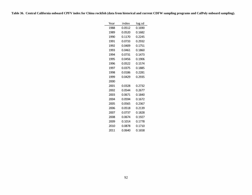
Table 36. Central California onboard CPFV index for China rockfish (data from historical and current CDFW sampling programs and CalPoly onboard sampling).

Year index log.sd1988 0.0512 0.16901989 0.0520 0.16821990 0.1170 0.22451991 0.0733 0.29321992 0.0409 0.17511993 0.0461 0.18601994 0.0731 0.14731995 0.0456 0.19061996 0.0522 0.15741997 0.0375 0.18851998 0.0186 0.22811999 0.0429 0.293520002001 0.0328 0.27322002 0.0544 0.26772003 0.0671 0.18402004 0.0594 0.16722005 0.0565 0.23672006 0.0518 0.21392007 0.0737 0.18282008 0.0674 0.19272009 0.1014 0.17782010 0.0878 0.17102011 0.0640 0.1658

92

Table 37. Central California onboard CPFV index for copper rockfish (data from historical and current CDFW sampling programs and CalPoly onboard sampling).

Year index log.sd1988 0.0397 0.14161989 0.0597 0.11871990 0.0724 0.20051991 0.0468 0.22321992 0.0686 0.12071993 0.0697 0.12541994 0.0495 0.13291995 0.0603 0.12521996 0.0576 0.12081997 0.0604 0.12691998 0.0552 0.15181999 0.0403 0.408620002001 0.1001 0.21872002 0.0545 0.37422003 0.0736 0.19902004 0.0939 0.11752005 0.1555 0.12352006 0.1497 0.11042007 0.1309 0.11662008 0.0764 0.16362009 0.0705 0.17862010 0.1370 0.11262011 0.1029 0.1239

93

Table 38. Least square means of the delta-GLM for brown rockfish, southern area (CDFW Observer Program).

Year Index CV 1999 0.0089 0.377 2000 0.0055 0.419 2001 0.0079 0.403 2002 0.0229 0.213 2003 0.0299 0.205 2004 0.0193 0.245 2005 0.0366 0.166 2006 0.0857 0.124 2007 0.0550 0.139 2008 0.0815 0.120 2009 0.0647 0.109 2010 0.0826 0.113 2011 0.0577 0.154

Table 39. Least square means of the delta-GLM for copper rockfish, southern area (CDFW Observer Program).

Year Index CV 1999 0.0347 0.205 2000 0.0483 0.280 2001 0.0103 0.387 2002 0.0167 0.258 2003 0.0429 0.183 2004 0.0253 0.197 2005 0.0567 0.164 2006 0.0655 0.128 2007 0.1051 0.105 2008 0.0848 0.098 2009 0.0611 0.121 2010 0.0553 0.110 2011 0.0815 0.096

94

Table 40. Least square means of the delta-GLM for China rockfish, northern area (ODFW Observer Program). Year Index CV 2001 0.0341 0.241 2002 2003 0.0306 0.220 2004 0.0205 0.332 2005 0.0154 0.345 2006 0.0189 0.276 2007 0.0369 0.199 2008 0.0178 0.274 2009 0.0300 0.242 2010 0.0081 0.542 2011 0.0236 0.439 2012 0.0334 0.262

Table 41. Least square means of the delta-GLM for copper rockfish, northern area (ODFW Observer Program).

Year Index CV 2001 0.0264 0.350 2002 2003 0.0147 0.369 2004 0.0118 0.423 2005 0.0387 0.308 2006 0.0384 0.261 2007 0.0304 0.237 2008 0.0149 0.324 2009 0.0316 0.290 2010 0.0406 0.304 2011 0.0137 0.513 2012 0.0230 0.365

95

Table 42. Sex-specific priors for natural mortality (M) calculated from Hamel’s method and used in exSSS sensitivity runs. M is given in normal space, but the prior is lognormal, with SD log the standard deviation in log space.

Females Males Group Species M SD log M SD log Rockfishes Brown 0.17 0.41 0.18 0.41

China 0.12 0.41 0.12 0.41 Copper 0.16 0.30 0.14 0.41 Sharpchin 0.13 0.41 0.14 0.41 Stripetail 0.17 0.41 0.21 0.41 Yellowtail N 0.14 0.30 0.11 0.41

Flatfishes English sole 0.33 0.26 0.41 0.33 Rex sole 0.31 0.33 0.31 0.33

96

7.2 Model results 7.2.1 XBD-SRA model estimates Table 43. Derived quantities from DB-SRA and XDB-SRA for three species of nearshore rockfishes. Parentheses contain the range of the 95% credibility intervals. * OFL estimates for Copper rockfish North and South of 40°10′ N. lat. are a post-stratification of assessment results based on cumulative removals by area, 1916-2012.

Stock SB0 SB2013 SB2013 / SB0 SBMSY F2012 / FMSY MSY OFL2015 OFL2016

Brown rockfish (Coastwide) 2046 (880 - 5697) 784 (56 - 3920) 0.42 (0.03 - 0.88) 818 (352 - 2279) 0.67 (0.19 - 10.18) 145 (63 - 253) 151 (1 - 513) 149 (0 - 508)China rockfish (N. of 40°10' N. lat.) 225 (116 - 614) 57 (2 - 448) 0.27 (0.01 - 0.79) 90 (46 - 245) 3.46 (0.39 - 38.92) 8 (2 - 23) 4 (0 - 44) 4 (0 - 45)China rockfish (S. of 40°10' N. lat.) 624 (276 - 1722) 199 (10 - 1250) 0.35 (0.02 - 0.85) 249 (111 - 689) 0.85 (0.14 - 16.34) 21 (7 - 48) 17 (0 - 98) 15 (0 - 96)Copper rockfish (N. of 34°27' N. lat.) 2023 (965 - 5388) 787 (53 - 3904) 0.41 (0.03 - 0.92) 809 (386 - 2155) 0.48 (0.11 - 8.03) 100 (36 - 188) 100 (3 - 422) 97 (0 - 409)Copper rockfish (S. of 34°27' N. lat.) 1110 (576 - 2886) 423 (27 - 2116) 0.4 (0.03 - 0.9) 444 (230 - 1154) 0.98 (0.2 - 14.37) 56 (19 - 112) 52 (1 - 244) 46 (0 - 226)

Stock SB0 SB2013 SB2013 / SB0 SBMSY F2012 / FMSY MSY OFL2015 OFL2016

Brown rockfish (Coastwide) 1794 (977 - 3732) 727 (333 - 2285) 0.42 (0.22 - 0.77) 718 (391 - 1493) 0.63 (0.27 - 1.47) 149 (109 - 196) 166 (69 - 364) 162 (66 - 361)China rockfish (N. of 40°10' N. lat.) 243 (127 - 542) 84 (22 - 366) 0.37 (0.12 - 0.73) 97 (51 - 217) 2.15 (0.49 - 11.29) 9 (3 - 20) 7 (1 - 35) 7 (1 - 36)China rockfish (S. of 40°10' N. lat.) 405 (232 - 1272) 264 (138 - 925) 0.66 (0.4 - 0.93) 162 (93 - 509) 0.27 (0.13 - 0.58) 32 (22 - 50) 55 (25 - 108) 53 (23 - 104)Copper rockfish (N. of 34°27' N. lat.) 1704 (1081 - 2734) 795 (417 - 1694) 0.48 (0.26 - 0.85) 681 (433 - 1093) 0.34 (0.15 - 0.87) 114 (75 - 148) 145 (56 - 314) 141 (52 - 308)Copper rockfish (S. of 34°27' N. lat.) 942 (545 - 2745) 699 (351 - 2189) 0.76 (0.43 - 0.99) 377 (218 - 1098) 0.32 (0.16 - 0.86) 84 (51 - 136) 167 (59 - 303) 154 (54 - 287)Copper rockfish (N. of 40°10' N. lat.) 11* 10*Copper rockfish (S. of 40°10' N. lat.) 301* 284*

DB-SRA (catch-based) estimates

XDB-SRA estimates

97

7.2.1.1 Brown rockfish Table 44. Time series from the XDB-SRA model for brown rockfish. Derived quantities (biomasses, depletion, and exploitation rates) are median values. Catch is total catch (landings + discard).

Year Catch Vulnerable Biomass Spawning Biomass Depletion Exploitation Rate Exp. Rate / Emsy1916 9.2 3588.2 1794.1 1.000 0.003 0.0241917 14.3 3579.0 1789.5 0.997 0.004 0.0371918 16.7 3565.8 1782.9 0.994 0.005 0.0441919 11.6 3551.8 1775.9 0.990 0.003 0.0301920 11.9 3545.2 1772.6 0.988 0.003 0.0311921 9.8 3539.2 1769.6 0.986 0.003 0.0261922 8.4 3536.1 1768.0 0.985 0.002 0.0221923 9.1 3536.1 1768.1 0.985 0.003 0.0241924 5.3 3535.2 1767.6 0.985 0.001 0.0141925 7.6 3537.7 1768.9 0.986 0.002 0.0201926 9.6 3536.8 1768.4 0.986 0.003 0.0251927 4.3 3534.1 1767.0 0.985 0.001 0.0111928 5.7 3536.7 1768.4 0.986 0.002 0.0151929 5.4 3537.6 1768.8 0.986 0.002 0.0141930 10.5 3538.0 1769.0 0.986 0.003 0.0271931 13.8 3533.2 1766.6 0.985 0.004 0.0361932 14.3 3526.1 1763.1 0.983 0.004 0.0381933 15.8 3519.4 1759.7 0.981 0.004 0.0421934 11.2 3511.8 1755.9 0.979 0.003 0.0301935 14.4 3508.9 1754.4 0.979 0.004 0.0381936 15.0 3503.1 1751.6 0.978 0.004 0.0401937 17.0 3498.6 1749.3 0.977 0.005 0.0451938 18.3 3493.1 1746.6 0.975 0.005 0.0491939 20.1 3486.2 1743.1 0.973 0.006 0.0541940 22.3 3478.0 1739.0 0.971 0.006 0.0601941 22.0 3468.5 1734.2 0.969 0.006 0.0591942 6.7 3460.1 1730.0 0.967 0.002 0.0181943 8.7 3468.2 1734.1 0.969 0.003 0.0231944 5.6 3473.3 1736.6 0.971 0.002 0.0151945 12.2 3479.5 1739.8 0.973 0.004 0.0331946 23.0 3479.8 1739.9 0.973 0.007 0.0611947 14.0 3469.2 1734.6 0.970 0.004 0.0371948 22.5 3468.9 1734.5 0.970 0.006 0.0601949 29.8 3459.9 1730.0 0.968 0.009 0.0801950 30.2 3444.6 1722.3 0.964 0.009 0.0811951 46.1 3430.4 1715.2 0.960 0.013 0.1241952 46.6 3402.2 1701.1 0.951 0.014 0.1271953 37.1 3376.4 1688.2 0.944 0.011 0.1021954 50.9 3364.4 1682.2 0.941 0.015 0.1401955 99.2 3339.5 1669.8 0.934 0.030 0.2751956 106.3 3270.8 1635.4 0.915 0.032 0.3021957 108.6 3204.3 1602.1 0.896 0.034 0.3151958 129.4 3142.9 1571.5 0.879 0.041 0.3831959 91.0 3069.0 1534.5 0.858 0.030 0.2761960 106.3 3038.6 1519.3 0.851 0.035 0.3261961 85.3 3000.3 1500.1 0.841 0.028 0.2641962 92.2 2985.4 1492.7 0.838 0.031 0.2871963 116.4 2966.5 1483.2 0.833 0.039 0.3641964 94.2 2924.8 1462.4 0.822 0.032 0.298

98

Table 44. (Continued). Time series from the XDB-SRA model for brown rockfish. Derived quantities (biomasses, depletion, and exploitation rates) are median values. Catch is total catch (landings + discard).


99

Table 45. Percentiles of estimated parameters and derived quantities from the XDB-SRA model for brown rockfish (coastwide). OFL estimates after 2013 assume projections of constant catch, equal to average catch from 2010-2012.

Quantity Derived or Estimated 5% 25% 50% 75% 95%log q (index 1) Derived -9.257 -8.580 -8.188 -7.849 -7.411log q (index 2) Derived -11.535 -10.871 -10.487 -10.143 -9.715log q (index 3) Derived -10.052 -9.387 -9.015 -8.709 -8.313log q (index 4) Derived -12.361 -11.704 -11.336 -11.033 -10.640log a (index 1) Estimated -3.703 -3.056 -2.649 -2.286 -1.786log a (index 2) Estimated -1.021 -0.537 -0.201 0.149 0.689log a (index 3) Estimated -2.375 -1.592 -1.117 -0.703 -0.163log a (index 4) Estimated -2.693 -1.545 -0.954 -0.490 0.121M Estimated 0.074 0.104 0.133 0.170 0.243FMSY / M Estimated 0.532 0.764 0.971 1.209 1.687Delta (year: 2000) Estimated 0.440 0.612 0.698 0.767 0.833BMSY / B0 Estimated 0.221 0.318 0.399 0.483 0.609FMSY Derived 0.066 0.101 0.130 0.165 0.236EMSY Derived 0.060 0.091 0.114 0.141 0.191MSY Derived 124.1 141.5 155.7 170.5 197.9BMSY Derived 848.6 1120.9 1383.4 1694.4 2463.8Vulnerable Biomass (1916) Derived 2194.4 2918.0 3588.2 4368.4 6254.6Vulnerable Biomass (2015) Derived 811.6 1143.2 1523.7 2081.9 3632.5OFL 2015 Derived 101.6 136.3 170.9 217.2 350.6

Percentile

100

Table 46. Sensitivity analyses for brown rockfish (coastwide) presented at the STAR Panel. Results are not based on the final (base) model. ‘oldBase’ uses productivity priors from Dick and MacCall (2010), ‘Zhou’ uses diffuse priors for FMSY/M and BMSY/B0 (see text for details), and runs starting with ‘Z-’ are the ‘Zhou’ run fit to single indices of abundance.

Run SB0 SB2013 SB2013/SB0 F2012/FMSY OFL2015 OFL2016

oldBase 1839.1 (1279.8 - 2853.3) 570.5 (326.9 - 1344.3) 0.32 (0.21 - 0.54) 0.81 (0.45 - 1.3) 123.9 (78.6 - 217.5) 126.2 (79.5 - 221.1)Zhou 1791.4 (1139.5 - 2853.7) 507.8 (287 - 1312.8) 0.3 (0.17 - 0.57) 0.77 (0.41 - 1.23) 132.8 (84.4 - 236.2) 136.2 (85.5 - 241.6)

Z-CenCalObsOnly 2321.8 (1389 - 5753.4) 1007.1 (381.3 - 4071.1) 0.45 (0.22 - 0.81) 0.57 (0.15 - 1.15) 171.9 (87.5 - 613) 175 (88.2 - 614.7)Z-SoCalObsOnly 1787.9 (779.2 - 105112) 770.8 (320.8 - 97210.3) 0.53 (0.19 - 0.97) 0.35 (0 - 1.38) 279.4 (71.5 - 13940.9) 286.3 (71.4 - 13044.9)Z-RecFINONly 2370.8 (1216.8 - 4298.7) 431.2 (146.6 - 1666.2) 0.2 (0.07 - 0.51) 1.4 (0.39 - 5.39) 71 (14.3 - 241.8) 70.7 (11.7 - 246.2)

101

7.2.1.2 China rockfish

7.2.1.2.1 North of 40° 10′ N lat. Table 47. Time series from the XDB-SRA model for China rockfish (north of 40° 10′ N lat.). Derived quantities (biomasses, depletion, and exploitation rates) are median values. Catch is total catch (landings + discard).


102

Table 47 (Continued). Time series from the XDB-SRA model for China rockfish (north of 40° 10′ N lat.). Derived quantities (biomasses, depletion, and exploitation rates) are median values. Catch is total catch (landings + discard).


103

Table 48. Percentiles of estimated parameters and derived quantities from the XDB-SRA model for China rockfish (north of 40° 10′ N lat.). OFL estimates assume projections of constant catch, equal to average catch from 2010-2012.

Quantity Derived or Estimated 5% 25% 50% 75% 95%log q (index 1) Derived -9.970 -9.429 -9.168 -8.902 -8.561log q (index 2) Derived -10.160 -9.468 -9.085 -8.728 -8.271log a (index 1) Estimated -4.635 -3.336 -2.712 -2.173 -1.512log a (index 2) Estimated -3.962 -2.669 -1.987 -1.386 -0.621M Estimated 0.030 0.044 0.058 0.075 0.108FMSY / M Estimated 0.431 0.678 0.916 1.271 1.931Delta (year: 2000) Estimated 0.265 0.387 0.461 0.517 0.585BMSY / B0 Estimated 0.195 0.298 0.381 0.475 0.605FMSY Derived 0.019 0.035 0.054 0.080 0.136EMSY Derived 0.019 0.034 0.051 0.074 0.122MSY Derived 3.82 6.78 9.48 12.22 17.98BMSY Derived 99.2 138.2 178.7 230.6 347.6Vulnerable Biomass (1916) Derived 280.6 388.0 486.0 599.6 910.8Vulnerable Biomass (2015) Derived 43.7 98.7 157.9 257.0 539.1OFL 2015 Derived 1.62 4.58 8.13 14.12 30.19

Percentile

104

Table 49. Sensitivity analyses for China rockfish (north of 40° 10′ N lat.) presented at the STAR Panel. Results are not based on the final (base) model. ‘oldBase’ uses productivity priors from Dick and MacCall (2010), ‘Zhou’ uses diffuse priors for FMSY/M and BMSY/B (see text for details), and runs starting with ‘Z-’ are the ‘Zhou’ run fit to single indices of abundance.

Run SB0 SB2013 SB2013/SB0 F2012/FMSY OFL2015 OFL2016oldBase 231 (154.9 - 397.2) 80.6 (28.9 - 249.2) 0.36 (0.16 - 0.65) 2.37 (0.75 - 6.98) 6.7 (1.7 - 22.4) 6.4 (1.4 - 22.3)

Zhou 227.4 (131 - 404.2) 80.6 (28.5 - 250.6) 0.37 (0.16 - 0.67) 2.06 (0.57 - 7.53) 7.7 (1.7 - 29.2) 7.4 (1.3 - 29.1)Z-NorCalORObsOnly 237.1 (128.5 - 533.7) 89.8 (25.7 - 379) 0.4 (0.15 - 0.78) 1.87 (0.41 - 7.13) 8.5 (1.7 - 41.3) 8.3 (1.3 - 41.3)

Z-RecFINOnly 221.7 (133 - 396.5) 66.8 (22.5 - 240.2) 0.32 (0.12 - 0.67) 2.63 (0.6 - 10.02) 5.8 (1 - 27.9) 5.5 (0.7 - 27.7)

105

7.2.1.2.2 South of 40° 10′ N lat. Table 50. Time series from the XDB-SRA model for China rockfish (south of 40° 10′ N lat.). Derived quantities (biomasses, depletion, and exploitation rates) are median values. Catch is total catch (landings + discard).


106

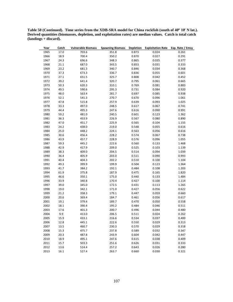
Table 50 (Continued). Time series from the XDB-SRA model for China rockfish (south of 40° 10′ N lat.). Derived quantities (biomasses, depletion, and exploitation rates) are median values. Catch is total catch (landings + discard).


107

Table 51. Percentiles of estimated parameters and derived quantities from the XDB-SRA model for China rockfish (south of 40° 10′ N lat.). OFL estimates assume projections of constant catch, equal to average catch from 2010-2012.


Percentile

108

Table 52. Sensitivity analyses for China rockfish (south of 40° 10′ N lat.) presented at the STAR Panel. Results are not based on the final (base) model. ‘oldBase’ uses productivity priors from Dick and MacCall (2010), ‘Zhou’ uses diffuse priors for FMSY/M and BMSY/B0 (see text for details), and runs starting with ‘Z-’ are the ‘Zhou’ run fit to single indices of abundance.

Run SB0 SB2013 SB2013/SB0 F2012/FMSY OFL2015 OFL2016

oldBase 747.9 (382.9 - 2166.9) 463.2 (202.9 - 1818.8) 0.65 (0.45 - 0.87) 0.29 (0.1 - 0.58) 47.4 (24 - 139.4) 47.9 (24.2 - 139.8)Zhou 463.9 (264.1 - 2050.1) 310.8 (164.8 - 1666.3) 0.69 (0.45 - 0.93) 0.27 (0.1 - 0.5) 52.5 (28.3 - 142.4) 53.4 (28.8 - 142.7)

Z-CenCalObsOnly 387.5 (240.9 - 1024) 201.8 (114.6 - 663) 0.53 (0.33 - 0.82) 0.34 (0.18 - 0.63) 41.9 (22.9 - 77.8) 43.1 (23.3 - 78.5)Z-RecFINOnly 1166.4 (463 - 4426.6) 710.4 (230.2 - 3888.4) 0.67 (0.34 - 0.93) 0.27 (0.06 - 1.04) 52.5 (13.4 - 263.8) 52.7 (13.3 - 263.8)

109

7.2.1.3 Copper rockfish

7.2.1.3.1 North of 34° 27′ N lat. Table 53. Time series from the XDB-SRA model for copper rockfish (north of 34° 27′ N lat.). Derived quantities (biomasses, depletion, and exploitation rates) are median values. Catch is total catch (landings + discard).


110

Table 53 (Continued). Time series from the XDB-SRA model for copper rockfish (north of 34° 27′ N lat.). Derived quantities (biomasses, depletion, and exploitation rates) are median values. Catch is total catch (landings + discard).


111

Table 54. Percentiles of estimated parameters and derived quantities from the XDB-SRA model for copper rockfish (north of 34° 27′ N lat.). OFL estimates assume projections of constant catch, equal to average catch from 2010-2012.

Quantity Derived or Estimated 5% 25% 50% 75% 95%log q (index 1) Derived -10.308 -9.805 -9.515 -9.243 -8.890log q (index 2) Derived -10.586 -10.074 -9.775 -9.507 -9.166log q (index 3) Derived -11.563 -11.118 -10.849 -10.592 -10.230log a (index 1) Estimated -3.430 -2.964 -2.613 -2.282 -1.794log a (index 2) Estimated -2.612 -1.981 -1.604 -1.251 -0.760log a (index 3) Estimated -3.753 -2.473 -1.861 -1.320 -0.708M Estimated 0.050 0.070 0.089 0.113 0.159FMSY / M Estimated 0.631 0.880 1.090 1.349 1.819Delta (year: 2000) Estimated 0.479 0.635 0.717 0.780 0.843BMSY / B0 Estimated 0.231 0.325 0.402 0.489 0.606FMSY Derived 0.054 0.079 0.099 0.121 0.164EMSY Derived 0.051 0.073 0.090 0.108 0.142MSY Derived 86.6 104.5 118.2 133.1 155.5BMSY Derived 839.5 1112.8 1334.4 1605.6 2119.9Vulnerable Biomass (1916) Derived 2333.0 2936.9 3407.3 3894.9 4964.6Vulnerable Biomass (2015) Derived 998.1 1369.7 1691.2 2142.1 3055.5OFL 2015 Derived 80.5 117.4 150.8 195.9 277.3

Percentile

112

Table 55. Sensitivity analyses for copper rockfish (preliminary coastwide model) presented at the STAR Panel. Results are not based on the final (base) model. ‘oldBase’ uses productivity priors from Dick and MacCall (2010), ‘Zhou’ uses diffuse priors for FMSY/M and BMSY/B0 (see text for details), and runs starting with ‘Z-’ are the ‘Zhou’ run fit to single indices of abundance.

Run SB0 SB2013 SB2013/SB0 F2012/FMSY OFL2015 OFL2016oldBase 2677.9 (1994.6 - 3868.9) 1150.8 (733.6 - 2184.5) 0.43 (0.31 - 0.64) 0.52 (0.31 - 0.82) 193.7 (123.4 - 319.1) 199 (126.2 - 323.7)

Zhou 2677.3 (1950.1 - 3902.7) 1202.2 (756.6 - 2253.2) 0.45 (0.3 - 0.73) 0.45 (0.25 - 0.77) 226.6 (134.3 - 388.4) 233.2 (138 - 395.7)Z-NorCalORObsOnly 3660.1 (2256.9 - 7057.9) 881.1 (187.2 - 4958.9) 0.26 (0.06 - 0.77) 1.23 (0.21 - 6.17) 80.7 (13.8 - 485.3) 81.6 (13 - 487.5)

Z-CenCalObsOnly 2334.6 (1722.1 - 3110.2) 1374.1 (746.3 - 2292.1) 0.59 (0.32 - 0.95) 0.31 (0.17 - 0.58) 327.8 (179.8 - 533.6) 337.1 (185.8 - 535.4)Z-SoCalObsOnly 2751.7 (1657.7 - 5519.9) 841.2 (247.2 - 3157.9) 0.32 (0.09 - 0.81) 0.68 (0.2 - 2.96) 150 (31.5 - 489.3) 155.3 (31 - 496.1)Z-RecFINONly 5185.6 (3063.8 - 10457.7) 1975.8 (861.5 - 7046.1) 0.4 (0.23 - 0.72) 0.71 (0.17 - 1.97) 139.8 (49.3 - 606.4) 140.9 (49.1 - 606.2)

113

7.2.1.3.2 South of 34° 27′ N lat. Table 56. Time series from the XDB-SRA model for copper rockfish (south of 34° 27′ N lat.). Derived quantities (biomasses, depletion, and exploitation rates) are median values. Catch is total catch (landings + discard).


114

Table 56 (Continued). Time series from the XDB-SRA model for copper rockfish (south of 34° 27′ N lat.). Derived quantities (biomasses, depletion, and exploitation rates) are median values. Catch is total catch (landings + discard).


115

Table 57. Percentiles of estimated parameters and derived quantities from the XDB-SRA model for copper rockfish (south of 34° 27′ N lat.). OFL estimates assume projections of constant catch, equal to average catch from 2010-2012.


Percentile

116

7.2.2 ExSSS model estimates Table 58. Catchability coefficient (q) and the added variance values for each survey estimated in the MLE exSSS. X: not an applicable index. NA: not available due to unrealistic models.

Rockfishes Flatfishes

Survey Parameter Sharpchin Yellowtail N English sole Rex sole early Triennial q 1.35 NA 1.54 10.41

+ var NA NA 0.10 0.14 late Triennial q 0.53 NA 1.52 6.31

+ var NA NA 0.10 0.07 late Triennial q NA 0.54 NA NA

+ var NA 0.24 NA NA NWFSC annual q 6.89 0.22 1.22 1.79

+ var NA 0.02 0.29 0.00

117

Table 59. Results (reported as median values with 95% credibility intervals) of 5 derived outputs (Spawning biomass in the initial year (SB0) and in 2013 (SB2013), stock depletion status (SB2013/SB0), fishing status relative to MSY (F2012/FMSY), and OFLs in 2015 and 2016) for SSS and exSSS models.

Model Group Species SB0 SB2013 SB2013/SB0 F2012/FMSY OFL2015 OFL2016

exSSS AIS Rockfishes Sharpchin 7887 (2437-24724) 4947 (1456-21157) 0.680 (0.31-0.91) 0.02 416 (130-1474) 404 (132-1397)Yellowtail (N) 82974 (19363-277492) 50043 (12184-221920) 0.667 (0.35-0.90) 0.11 7218 (2646-23903) 6949 (2679-22724)

Flatfishes English sole 29238 (11757-94321) 25719(10444-89100) 0.879 (0.77-0.96) 0.013 10792 (7138-32391) 7890 (4921-23317)Rex sole 3808 (731-15814) 2966 (602-13150) 0.800 (0.64-0.93) 0.07 5764 (3089-16500) 3956 (2479-10253)

SSS Rockfishes Sharpchin 6204 (2273-13363) 3774 (1587-9595) 0.64 (0.39-0.87) 0.02 (0.01-0.05) 377 (158-854) 367 (159-806)Yellowtail (N) 54823 (10668-148869) 26819 (5673-101254) 0.56 (0.23-0.82) 0.17 (0.07-0.56) 4429 (1737-11083) 4378 (1848-10640)

Flatfishes English sole 32846 (7663-109934) 29368 (6562-102956) 0.89 (0.8-0.96) 0.01 (0-0.02) 13005 (6362-37567) 9274 (4149-27476)Rex sole 10529 (2009-37874) 7950 (1705-32430) 0.82 (0.66-0.95) 0.07 (0.02-0.11) 5956 (3552-22694) 4682 (2896-17218)

Derived Outputs

118

7.2.2.1 Sharpchin rockfish Table 60. Results of base case and sensitivity runs for sharpchin rockfish using exSSS. * indicate runs that did not converge. Colored cells indicate inclusion in the model run. Gray cells indicate indices wherein additional variance was estimated.

BC 1 2 3 4 5 5 7Index NWFSC

Triennial- earlyTriennial- late

Parameter treatment M- HoenigM-HamelNew h priorOld h prior

Parameter estimates MF 0.08 0.08 * 0.08 0.07 0.06 0.12 0.08MM 0.08 0.08 * 0.08 0.08 0.07 0.13 0.08h 0.95 0.95 * 0.95 0.95 0.92 0.95 0.75ln(R0) 9.16 8.88 * 8.67 8.19 7.87 9.66 8.84

Derived outputs SB0 16208 12210 * 9803 6464 5957 11360 11649SB2013 14426 10422 * 8013 4449 3208 10511 9580SB2013/SB0 0.89 0.85 * 0.82 0.69 0.54 0.93 0.82F2012/FMSY 0.00 0.00 * 0.00 0.01 0.02 0.00 0.01MSY 1004 761 * 616 386 286 1106 550OFL2015 1235 905 * 708 390 247 1311 829OFL2016 1181 868 * 681 379 244 1221 796

Model attributesSensitivity run

119

7.2.2.2 Yellowtail rockfish (North of 40° 10′ N lat.) Table 61. Results of base case and sensitivity runs for yellowtail rockfish (North of 40° 10’ N lat.) using exSSS. Colored cells indicate inclusion in the model run. Gray cells indicate indices wherein additional variance was estimated.

BC 1 2 3 4 5 6 7 8 9Index Triennial

NWFSCTriennial- earlyTriennial- late

Parameter treatment M- HoenigM-HamelNew h priorOld h prior

Parameter estimates MF 0.11 0.10 0.11 0.11 0.11 0.11 0.10 0.11 0.13 0.11MM 0.11 0.10 0.11 0.11 0.11 0.11 0.11 0.11 0.10 0.11h 0.95 0.94 0.95 0.95 0.95 0.96 0.93 0.95 0.95 0.75ln(R0) 10.28 9.82 9.84 11.66 9.82 9.73 10.25 9.80 10.37 10.27

Derived outputs SB0 102112 73960 63927 395204 68112 55206 96871 64878 74942 100759SB2013 84449 52848 45693 378844 48643 37020 76057 45706 64913 79383SB2013/SB0 0.83 0.71 0.71 0.96 0.71 0.67 0.79 0.70 0.87 0.79F2012/FMSY 0.03 0.06 0.05 0.01 0.06 0.06 0.05 0.06 0.03 0.07MSY 11172 7318 7146 44268 7220 6348 10154 7005 11775 8233OFL2015 12281 7080 7193 56591 6900 5641 9510 6582 15153 11981OFL2016 11647 6830 6894 52816 6650 5467 9191 6350 14128 11357

Model attributesSensitivity run

120

7.2.2.3 English sole Table 62. Results of base case and sensitivity runs for English sole using exSSS. Colored cells indicate inclusion in the model run. Gray cells indicate indices wherein additional variance was estimated.

BC 1 2 3 4 5 6 7Index Triennial- early

Triennial- lateNWFSCTriennial

Parameter treatment M- HoenigM-Hamel

Parameter MF 0.26 0.22 0.27 0.22 0.20 0.21 0.28 0.32MM 0.26 0.05 0.29 0.23 0.25 0.27 0.28 0.40h 0.80 0.86 0.89 0.74 0.82 0.88 0.85 0.83ln(R0) 11.62 11.08 11.51 11.40 11.50 11.21 11.62 11.91

Derived outputs SB0 29349 24625 24714 33666 45715 32891 25567 23263SB2013 26152 21679 22096 17437 40943 28014 22922 21252SB2013/SB0 0.89 0.88 0.89 0.52 0.90 0.85 0.90 0.91F2012/FMSY 0.02 0.01 0.01 0.04 0.01 0.01 0.01 0.01MSY 4136 4763 4143 3590 4885 3943 4146 4259OFL2015 12092 10767 10477 8237 14629 10384 11220 11901OFL2016 8493 8451 7286 10943 10943 7790 7739 7726

Sensitivity runModel attributes

121

7.2.2.4 Rex sole Table 63. Results of base case and sensitivity runs for rex sole using exSSS. * indicate runs that did not converge. Colored cells indicate inclusion in the model run. Gray cells indicate indices wherein additional variance was estimated.

BC 1 2 3 4 5 6 7Index Triennial- early

Triennial- lateNWFSCTriennial

Parameter treatment M- HoenigM-Hamel

Parameter MF 0.20 0.24 0.24 0.20 * 0.24 0.27 0.31MM 0.19 0.20 0.22 0.20 * 0.20 0.24 0.29h 0.80 0.90 0.84 0.79 * 0.89 0.91 0.84ln(R0) 9.97 9.75 10.20 9.91 * 9.75 10.11 10.28

Derived outputs SB0 8162 4196 6403 7364 * 4116 4474 3768SB2013 6474 2978 5233 4348 * 2915 3543 2790SB2013/SB0 0.79 0.71 0.82 0.59 * 0.71 0.79 0.74F2012/FMSY 0.07 0.09 0.07 0.12 * 0.09 0.07 0.10MSY 1956 1581 2107 1699 * 1578 1934 1656OFL2015 5609 3262 5056 3600 * 3304 3969 3505OFL2016 4259 2614 3949 3017 * 2643 3081 2717

Sensitivity runModel attributes

122

7.2.2.5 Stripetail rockfish Table 64. XDB-SRA results from a profile over credible values of log(q) for fishery-independent survey indices in the model. Depletion (B2013/B0) and F/FMSY estimates include median (50%) and 90% interval estimates. MSY and OFL (2015) estimates are median values of the posterior distributions.

MSY OFL15lnq 5% 50% 95% 5% 50% 95% 50% 50%-1 0.951 0.978 0.999 0.002 0.005 0.014 643 2341

-0.5 0.900 0.965 0.994 0.002 0.006 0.016 445 15900 0.872 0.942 0.998 0.003 0.009 0.023 247 845

0.5 0.810 0.909 0.998 0.004 0.011 0.033 162 5401 0.754 0.894 0.992 0.005 0.014 0.037 132 393

1.5 0.602 0.775 0.991 0.009 0.025 0.073 68 202

B2013/B0 F/Fmsy

123

7.2.3 Decision tables Table 65. Decision table for brown rockfish (coastwide), as presented during the STAR panel. Alternative catch streams are median ABC catch projections (mt) with 40-10 adjustment based on quartiles of depletion in 2013. SSB is median female spawning stock biomass. “Depl” is median depletion, and “Overfished” is the percentage of trajectories below 0.25B0. See the Executive Summary (Table ES2) for final base case model results.

Year Catch SSB Depl Overfished SSB Depl Overfished SSB Depl Overfished2013 101.5 480 0.29 23% 740 0.42 0% 1193 0.63 0%2014 101.5 493 0.30 19% 758 0.43 0% 1212 0.64 0%2015 101.5 506 0.30 17% 774 0.45 0% 1232 0.65 0%2016 101.5 521 0.31 13% 789 0.46 0% 1249 0.67 0%2017 101.5 534 0.32 9% 807 0.47 0% 1264 0.68 0%2018 101.5 547 0.32 8% 824 0.48 0% 1280 0.69 0%2019 101.5 561 0.33 6% 842 0.49 0% 1295 0.70 0%2020 101.5 576 0.34 5% 861 0.50 0% 1309 0.71 0%2021 101.5 590 0.34 4% 877 0.51 0% 1323 0.72 0%2022 101.5 605 0.35 3% 894 0.52 0% 1340 0.73 0%2023 101.5 620 0.36 3% 912 0.53 0% 1353 0.74 0%2024 101.5 634 0.36 3% 927 0.53 0% 1366 0.74 0%

Year Catch SSB Depl Overfished SSB Depl Overfished SSB Depl Overfished2013 101.5 480 0.29 23% 740 0.42 0% 1193 0.63 0%2014 101.5 493 0.30 19% 758 0.43 0% 1212 0.64 0%2015 103 506 0.30 17% 774 0.45 0% 1232 0.65 0%2016 107 520 0.31 15% 788 0.45 0% 1249 0.67 0%2017 111 531 0.32 13% 803 0.46 0% 1260 0.68 0%2018 114 539 0.32 12% 816 0.47 0% 1272 0.69 0%2019 117 548 0.32 11% 829 0.48 0% 1282 0.70 0%2020 119 557 0.33 11% 841 0.49 0% 1290 0.70 0%2021 121 566 0.33 10% 851 0.49 0% 1297 0.71 0%2022 123 572 0.33 11% 860 0.50 0% 1305 0.71 0%2023 125 579 0.33 11% 870 0.50 0% 1312 0.72 0%2024 126 586 0.34 11% 878 0.51 0% 1316 0.72 0%



Mgmt. Action: Median

ABC

Mgmt. Action:

High ABC

STATE OF NATURE: DEPLETION IN 2013Lower Quartile Interquartile Range Upper Quartile

Mgmt. Action: Recent Catch

Mgmt. Action:

Low ABC

124

Table 66. Decision table for China rockfish (north of 40° 10′ N lat.), as presented during the STAR panel. Alternative catch streams are median ABC catch projections (mt) with 40-10 adjustment based on quartiles of depletion in 2013. SSB is median female spawning stock biomass, “Depl” is median depletion, and “Overfished” is the percentage of trajectories below 0.25B0. See the Executive Summary (Table ES3) for final base case model results.




Year Catch SSB Depl Overfished SSB Depl Overfished SSB Depl Overfished2013 15.1 46 0.22 72% 91 0.39 0% 184 0.59 0%2014 15.1 42 0.21 85% 89 0.38 0% 183 0.59 0%2015 18.4 39 0.19 97% 87 0.37 0% 182 0.59 0%2016 18.1 34 0.17 100% 83 0.35 7% 180 0.58 0%2017 17.9 30 0.14 100% 79 0.33 15% 176 0.57 0%2018 17.8 25 0.12 100% 75 0.32 23% 174 0.56 0%2019 17.6 21 0.10 100% 72 0.30 30% 171 0.56 0%2020 17.5 16 0.07 100% 68 0.29 36% 169 0.55 0%2021 17.4 11 0.05 100% 65 0.28 41% 167 0.55 0%2022 17.2 6 0.03 100% 62 0.26 46% 165 0.54 0%2023 17.1 tr tr 100% 58 0.25 51% 163 0.54 0%2024 17.0 tr tr 98% 55 0.23 55% 161 0.53 0%


ABC

Mgmt. Action:

High ABC

Lower Quartile Interquartile Range Upper Quartile


Mgmt. Action:

Low ABC

STATE OF NATURE: DEPLETION IN 2013

125

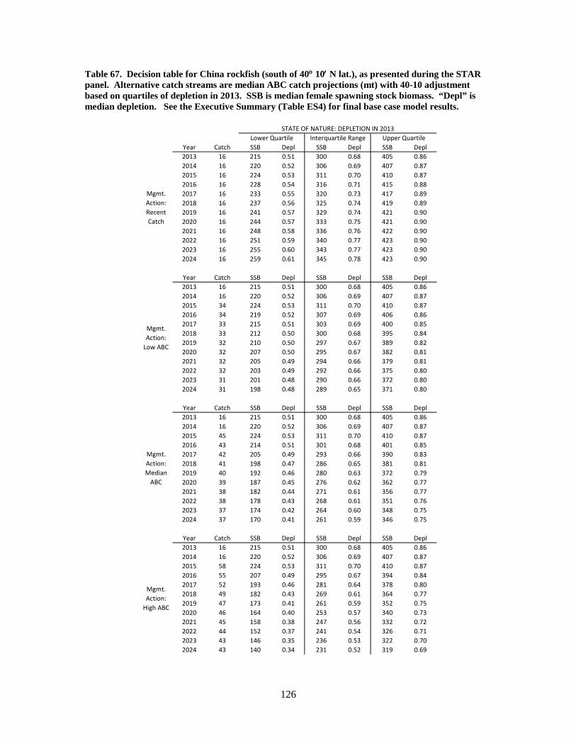
Table 67. Decision table for China rockfish (south of 40° 10′ N lat.), as presented during the STAR panel. Alternative catch streams are median ABC catch projections (mt) with 40-10 adjustment based on quartiles of depletion in 2013. SSB is median female spawning stock biomass. “Depl” is median depletion. See the Executive Summary (Table ES4) for final base case model results.

Year Catch SSB Depl SSB Depl SSB Depl2013 16 215 0.51 300 0.68 405 0.862014 16 220 0.52 306 0.69 407 0.872015 16 224 0.53 311 0.70 410 0.872016 16 228 0.54 316 0.71 415 0.882017 16 233 0.55 320 0.73 417 0.892018 16 237 0.56 325 0.74 419 0.892019 16 241 0.57 329 0.74 421 0.902020 16 244 0.57 333 0.75 421 0.902021 16 248 0.58 336 0.76 422 0.902022 16 251 0.59 340 0.77 423 0.902023 16 255 0.60 343 0.77 423 0.902024 16 259 0.61 345 0.78 423 0.90





ABC

Mgmt. Action:

High ABC



Mgmt. Action:

Low ABC

126

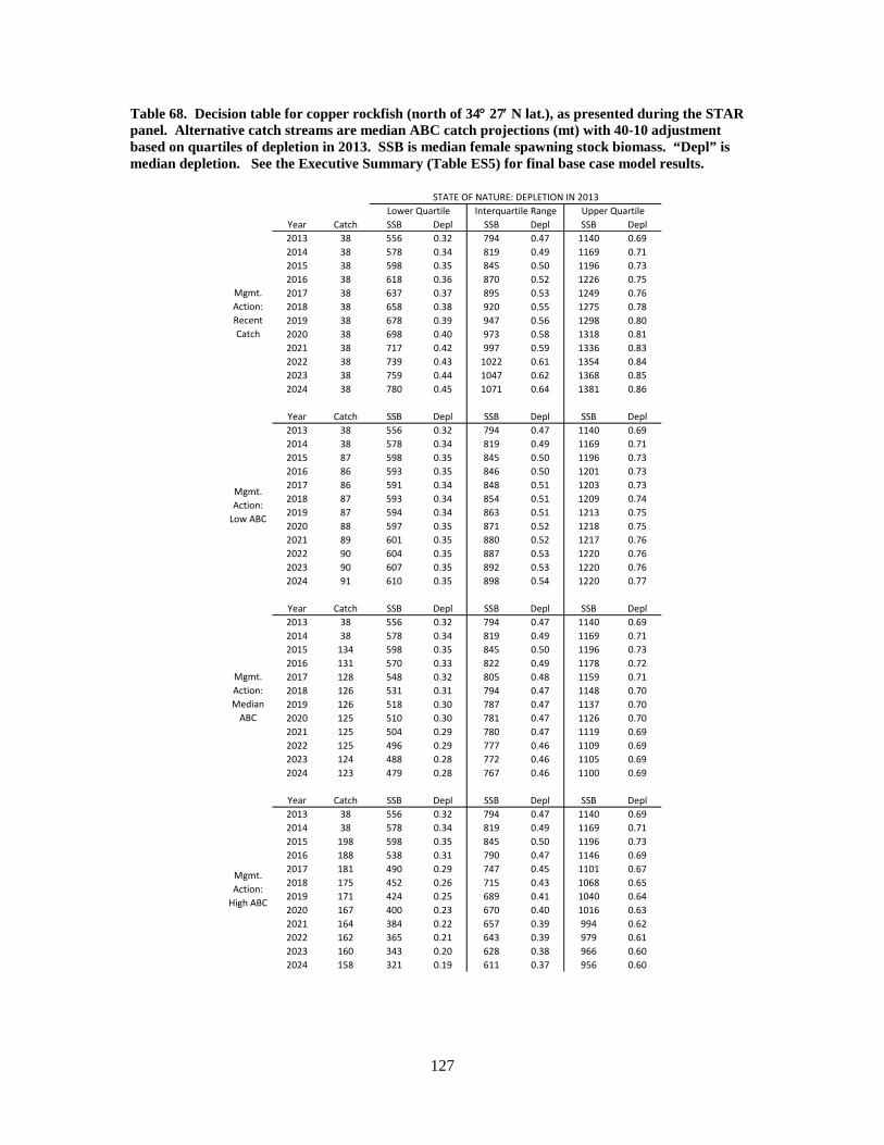
Table 68. Decision table for copper rockfish (north of 34° 27′ N lat.), as presented during the STAR panel. Alternative catch streams are median ABC catch projections (mt) with 40-10 adjustment based on quartiles of depletion in 2013. SSB is median female spawning stock biomass. “Depl” is median depletion. See the Executive Summary (Table ES5) for final base case model results.






ABC

Mgmt. Action:

High ABC



Mgmt. Action:

Low ABC

127

Table 69. Decision table for copper rockfish (south of 34° 27′ N lat.). Alternative catch streams are median ABC catch projections (mt) with 40-10 adjustment based on quartiles of depletion in 2013. SSB is median female spawning stock biomass. “Depl” is median depletion. See the Executive Summary (Table ES6) for final base case model results.





Mgmt. Action:

High ABC



Mgmt. Action:

Low ABC


ABC

128

Table 70. Decision table for sharpchin rockfish. Alternative catch streams are median ABC catch projections (mt) with 40-10 adjustment based on quartiles of depletion in 2013. “Spawning Biomass” is median female spawning stock biomass. “Depletion” is median depletion. Estimated MSY is 320 mt/year and the long-term average total yield based on SPR50% is 270 mt/year.




2015 195 3,485 51.5% 5,798 71.8% 7,904 86.3%2016 195 3,476 51.2% 5,791 71.6% 7,894 85.8%2017 194 3,469 50.9% 5,779 71.3% 7,881 85.4%2018 194 3,447 50.7% 5,762 71.1% 7,867 85.0%2019 193 3,440 50.4% 5,752 70.9% 7,852 84.8%2020 192 3,431 50.1% 5,743 70.6% 7,831 84.5%2021 191 3,426 49.9% 5,724 70.4% 7,798 84.2%2022 190 3,418 49.7% 5,705 70.2% 7,769 84.1%2023 189 3,401 49.5% 5,685 69.9% 7,744 83.8%2024 189 3,395 49.3% 5,667 69.8% 7,721 83.6%2015 382 3,371 51.1% 5,628 71.2% 7,561 86.0%2016 372 3,393 50.6% 5,531 69.5% 7,216 82.2%2017 363 3,394 50.1% 5,426 67.8% 6,908 78.4%2018 354 3,380 49.6% 5,300 66.1% 6,570 75.2%2019 347 3,377 49.2% 5,177 64.3% 6,313 72.5%2020 339 3,365 49.0% 5,091 62.7% 6,094 69.9%2021 334 3,363 48.6% 4,984 61.5% 5,895 67.5%2022 328 3,347 48.5% 4,933 60.4% 5,720 65.4%2023 322 3,321 48.3% 4,840 59.4% 5,561 63.8%2024 317 3,336 48.2% 4,770 58.5% 5,419 62.2%2015 750 3,343 50.6% 5,688 71.7% 7,863 86.0%2016 730 2,964 44.1% 5,338 66.4% 7,567 82.3%2017 703 2,594 38.6% 4,999 61.8% 7,310 87.7%2018 674 2,257 33.6% 4,643 57.2% 7,040 75.7%2019 650 1,953 28.9% 4,300 53.3% 6,791 73.1%2020 625 1,684 24.7% 4,001 49.6% 6,498 70.5%2021 612 1,392 20.8% 3,691 46.7% 6,215 68.6%2022 591 1,190 17.1% 3,479 43.6% 6,055 66.7%2023 575 980 13.9% 3,266 41.0% 5,935 65.0%2024 563 756 10.9% 3,095 38.6% 5,816 63.5%2015 5 3,485 50.6% 5,664 72.0% 7,573 86.4%2016 5 3,602 51.9% 5,786 73.4% 7,643 87.4%2017 5 3,725 53.7% 5,895 74.7% 7,708 88.2%2018 5 3,826 54.9% 6,020 75.9% 7,768 89.0%2019 5 3,938 56.3% 6,121 77.0% 7,828 89.7%2020 5 4,042 57.7% 6,227 78.3% 7,888 90.3%2021 5 4,135 59.0% 6,327 79.3% 7,944 91.1%2022 5 4,260 60.4% 6,420 80.3% 7,998 91.6%2023 5 4,318 61.6% 6,510 81.2% 8,048 92.2%2024 5 4,418 62.6% 6,599 82.2% 8,096 92.8%

0.25-0.75 0.75-1.0

State of nature

Low Catches

Medium Catches

High Catches

Average Catches

Low Base HighQuantiles 0-0.25

129

Table 71. Decision table for yellowtail rockfish (north of 40° 10′ N lat.). Alternative catch streams are median ABC catch projections (mt) with 40-10 adjustment based on quartiles of depletion in 2013. “Spawning Biomass” is median female spawning stock biomass. “Depletion” is median depletion. Estimated MSY is 5728 mt/year and the long-term average total yield based on SPR50% is 4805 mt/year.




2015 3,936 43,502 52.8% 56,604 68.9% 62,979 83.4%2016 3,912 43,108 52.4% 56,063 68.3% 62,573 82.7%2017 3,879 42,738 52.0% 55,772 67.9% 62,187 81.9%2018 3,844 42,434 51.7% 55,468 67.4% 61,835 81.2%2019 3,818 42,206 51.3% 55,027 66.7% 61,524 80.6%2020 3,797 41,976 50.9% 54,624 66.4% 61,253 79.9%2021 3,777 41,749 50.6% 54,269 66.0% 61,019 79.6%2022 3,759 41,547 50.4% 53,958 65.7% 60,818 79.3%2023 3,744 41,393 50.1% 53,684 65.3% 60,644 79.0%2024 3,730 41,129 50.0% 53,444 64.9% 60,491 78.8%

6,497 43,502 52.4% 54,304 69.3% 60,039 83.3%2016 6,312 43,252 52.1% 52,730 66.8% 55,750 87.0%2017 6,126 43,044 51.6% 51,060 64.6% 52,853 73.9%2018 5,962 42,955 51.1% 49,531 62.7% 50,294 70.5%2019 5,798 42,673 50.7% 48,227 61.0% 48,062 67.2%2020 5,638 42,597 50.4% 47,111 49.4% 46,136 64.4%2021 5,523 42,567 50.0% 46,260 58.2% 44,484 62.3%2022 5,417 42,547 49.9% 45,421 57.1% 43,067 60.5%2023 5,324 42,842 49.7% 44,594 56.2% 41,784 59.9%2024 5,251 42,899 49.4% 43,788 55.4% 40,810 57.6%2015 11,666 44,076 52.6% 54,174 69.4% 63,587 83.7%2016 11,148 39,125 46.6% 49,654 63.4% 60,602 78.9%2017 10,530 34,591 41.3% 45,256 58.0% 57,730 75.1%2018 10,032 30,672 36.4% 41,696 53.4% 55,222 71.7%2019 9,675 26,968 31.9% 38,467 49.6% 53,091 68.6%2020 9,333 23,925 28.2% 35,708 46.2% 51,319 66.1%2021 9,052 20,975 25.1% 33,481 43.0% 49,975 63.9%2022 8,830 18,205 22.3% 31,248 40.4% 48,657 62.2%2023 8,547 15,740 19.5% 29,253 38.2% 47,106 60.6%2024 8,311 13,900 17.0% 27,694 36.4% 46,200 59.3%2015 1,376 45,023 52.7% 54,405 69.6% 61,190 83.7%2016 1,376 46,290 54.1% 55,352 70.7% 61,802 84.4%2017 1,376 47,532 55.4% 56,136 72.0% 62,370 84.9%2018 1,376 48,447 56.5% 56,980 72.9% 62,899 85.5%2019 1,376 49,334 57.7% 57,758 73.7% 63,390 86.1%2020 1,376 50,528 59.0% 58,506 74.6% 63,845 86.5%2021 1,376 51,821 59.9% 59,109 75.5% 64,267 86.9%2022 1,376 52,752 61.0% 59,675 76.2% 64,658 87.3%2023 1,376 53,532 62.1% 60,139 77.0% 65,020 87.6%2024 1,376 54,297 63.1% 60,643 77.7% 65,355 87.9%

0.25-0.75 0.75-1.0

Low Catches

Medium Catches

High Catches

Average Catches


Quantiles 0-0.25

130

Table 72. Decision table for English sole. Alternative catch streams are median ABC catch projections (mt) with 40-10 adjustment based on quartiles of depletion in 2013. “Spawning Biomass” is median female spawning stock biomass. “Depletion” is median depletion. Estimated MSY is 4072 mt/year and the long-term average total yield based on SPR25% is 3875 mt/year.




2015 8,909 33,061 86.2% 24,798 90.7% 24,306 94.0%2016 7,247 26,491 67.9% 18,414 67.2% 18,274 71.1%2017 6,146 21,871 56.6% 14,277 52.0% 14,593 56.8%2018 5,379 18,728 48.7% 11,709 42.6% 12,608 48.6%2019 4,858 16,631 43.3% 10,061 37.1% 11,880 44.2%2020 4,529 15,286 39.7% 9,293 34.0% 11,515 43.0%2021 4,305 14,401 97.2% 8,908 32.3% 11,386 42.1%2022 4,151 13,766 35.5% 8,606 31.3% 11,128 41.4%2023 4,018 13,279 34.3% 8,424 30.7% 11,077 41.8%2024 3,939 12,947 33.4% 8,319 30.2% 10,982 42.0%2015 9,452 33,131 86.2% 24,735 90.7% 24,844 94.1%2016 4,098 26,338 67.7% 18,131 65.7% 16,751 63.2%2017 5,733 61,662 55.5% 14,115 50.8% 12,720 47.3%2018 4,972 18,441 47.3% 11,791 42.4% 10,602 39.6%2019 4,574 16,343 42.0% 10,538 37.9% 9,587 36.0%2020 4,332 14,991 38.6% 9,810 65.4% 9,065 34.3%2021 4,184 41,092 36.4% 9,401 34.0% 8,727 33.2%2022 4,073 13,465 34.8% 9,096 33.1% 8,490 32.6%2023 3,992 13,008 33.7% 8,916 32.4% 8,428 32.1%2024 3,922 12,662 33.0% 8,768 31.9% 8,340 31.7%2015 11,901 32,854 86.3% 25,220 90.6% 25,473 94.1%2016 2,368 23,791 61.8% 16,600 59.1% 17,158 63.6%2017 6,790 23,311 60.9% 16,346 58.2% 17,307 63.7%2018 5,975 19,630 51.5% 13,092 46.5% 14,308 53.7%2019 5,691 16,975 44.7% 10,874 38.8% 12,784 47.7%2020 5,446 14,926 39.1% 9,324 33.2% 11,642 43.0%2021 5,258 13,185 34.9% 8,098 29.1% 10,594 40.1%2022 5,106 12,087 31.5% 7,196 26.3% 10,178 38.2%2023 5,007 11,004 28.6% 6,557 24.3% 9,903 36.7%2024 4,960 10,260 26.4% 6,114 22.6% 9,600 36.2%2015 224 33,061 85.9% 25,473 90.7% 25,687 94.0%2016 224 33,694 87.3% 24,996 91.8% 25,853 94.6%2017 224 34,117 88.5% 25,186 92.6% 25,981 95.1%2018 224 34,518 89.6% 25,377 93.3% 26,078 95.4%2019 224 34,916 90.6% 25,522 93.8% 26,153 95.7%2020 224 35,358 91.4% 25,635 94.3% 26,210 96.0%2021 224 35,746 92.1% 25,725 94.6% 26,253 96.0%2022 224 36,087 82.6% 25,798 94.9% 26,286 96.3%2023 224 36,387 93.2% 25,857 95.1% 26,312 96.4%2024 224 36,651 93.6% 25,904 95.3% 26,332 96.6%

0.25-0.75 0.75-1.0

Low Catches

Medium Catches

High Catches

Average Catches


Quantiles 0-0.25

131

Table 73. Decision table for rex sole. Alternative catch streams are median ABC catch projections (mt) with 40-10 adjustment based on quartiles of depletion in 2013. “Spawning Biomass” is median female spawning stock biomass. “Depletion” is median depletion. Estimated MSY is 1676 mt/year and the long-term average total yield based on SPR25% is 1646 mt/year.

State of nature Low Base High

Quantiles 0-0.25 0.25-0.75 0.75-1.0

Year Catch

Spawning

Biomass Depletio

n

Spawning

Biomass Depletio

n

Spawning

Biomass Depletio

n

Low Catches

2015 3,085 3,772 72.9% 3,377 80.7% 4,396 89.7% 2016 2,541 3,113 59.4% 2,837 68.8% 3,989 81.4% 2017 2,174 2,568 50.6% 2,490 60.8% 3,742 76.1% 2018 1,909 2,237 44.8% 2,262 55.7% 3,560 72.9% 2019 1,753 2,102 41.1% 2,137 52.6% 3,448 71.0% 2020 1,652 2,022 38.7% 2,031 50.6% 3,380 70.3% 2021 1,590 1,970 36.9% 1,986 49.3% 3,339 69.7% 2022 1,544 1,928 35.8% 1,939 48.5% 3,313 69.4% 2023 1,510 1,887 35.2% 1,924 48.1% 3,297 69.2% 2024 1,485 1,857 34.6% 1,917 47.9% 3,287 69.1%

Medium Catches

2015 4,395 3,788 73.4% 3,073 81.1% 4,076 89.5% 2016 3,342 3,023 59.5% 2,382 62.0% 2,937 64.7% 2017 2,701 2,569 50.4% 1,938 50.3% 2,313 50.7% 2018 2,308 2,279 44.3% 1,662 43.4% 1,963 43.3% 2019 2,067 2,086 40.5% 1,511 39.4% 1,765 39.2% 2020 1,926 1,940 38.1% 1,421 37.1% 1,663 36.9% 2021 1,839 1,859 36.5% 1,371 35.7% 1,602 35.7% 2022 1,778 1,812 35.6% 1,335 34.8% 1,562 34.9% 2023 1,738 1,784 34.9% 1,305 34.2% 1,517 34.3% 2024 1,711 1,764 34.4% 1,283 33.8% 1,496 33.8%

High Catches

2015 7,895 3,720 73.4% 3,073 81.1% 4,093 89.5% 2016 5,315 1,684 34.1% 1,717 44.9% 2,866 64.7% 2017 4,116 928 20.3% 973 27.4% 2,208 51.6% 2018 3,382 732 15.8% 731 21.0% 1,927 44.8% 2019 1,947 685 14.0% 655 18.9% 1,726 41.2% 2020 2,722 657 13.6% 641 18.7% 1,791 42.3% 2021 2,547 629 13.1% 605 17.5% 1,697 40.7% 2022 2,470 607 12.4% 571 16.4% 1,663 40.0% 2023 2,387 594 11.9% 552 15.6% 1,612 39.5% 2024 2,344 578 11.6% 542 15.2% 1,579 38.9%

Average Catches

2015 455 3,687 73.2% 3,158 81.0% 3,686 89.9% 2016 455 3,761 74.4% 3,191 81.9% 3,707 90.3% 2017 455 3,824 75.4% 3,220 82.6% 3,723 90.6% 2018 455 3,874 76.3% 3,245 83.2% 3,737 90.9% 2019 455 3,919 77.2% 3,266 83.7% 3,747 91.1% 2020 455 3,959 77.9% 3,285 84.2% 3,757 91.3% 2021 455 3,993 78.4% 3,301 84.6% 3,765 91.6% 2022 455 4,022 78.9% 3,315 84.9% 3,771 91.7% 2023 455 4,047 79.4% 330 85.2% 3,777 91.9% 2024 455 4,067 79.8% 3,340 85.5% 3,782 92.0%

132

8 Figures 8.1 Catch and Abundance Figures 8.1.1 Distribution maps

Figure 1. Occurrence and abundance of sharpchin rockfish found in the NWFSC annual survey (2003-2012) north of 40º10’ N lat.

133

Figure 2. Occurrence and abundance of sharpchin rockfish found in the NWFSC annual survey (2003-2012) south of 40º10’ N lat.

134

Figure 3. Occurrence and abundance of stripetail rockfish found in the NWFSC annual survey (2003-2012) north of 40º10’ N lat.

135

Figure 4. Occurrence and abundance of stripetail rockfish found in the NWFSC annual survey (2003-2012) south of 40º10’ N lat.

136

Figure 5. Occurrence and abundance of yellowtail rockfish found in the NWFSC annual survey (2003-2012) north of 40º10’ N lat.

137

Figure 6. Occurrence and abundance of yellowtail rockfish found in the NWFSC annual survey (2003-2012) south of 40º10’ N lat.

138

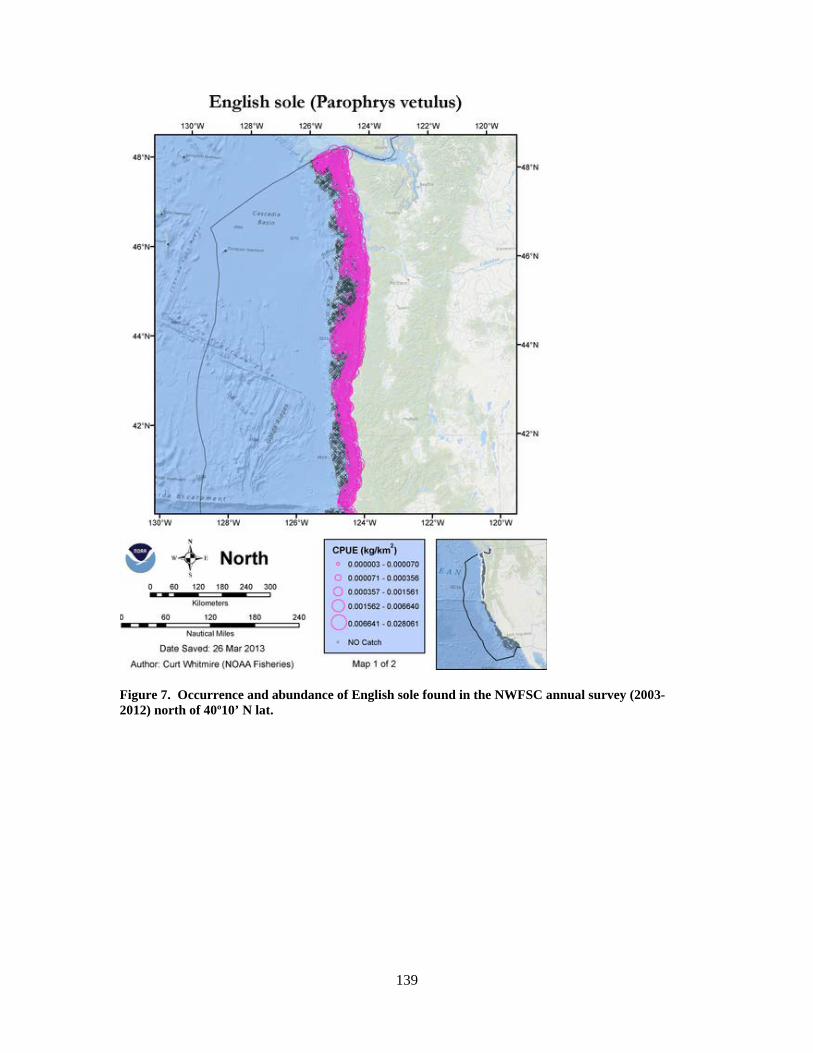
Figure 7. Occurrence and abundance of English sole found in the NWFSC annual survey (2003-2012) north of 40º10’ N lat.

139

Figure 8. Occurrence and abundance of English sole found in the NWFSC annual survey (2003-2012) south of 40º10’ N lat.

140

Figure 9. Occurrence and abundance of rex sole found in the NWFSC annual survey (2003-2012) north of 40º10’ N lat.

141

Figure 10. Occurrence and abundance of rex sole found in the NWFSC annual survey (2003-2012) south of 40º10’ N lat.

142

Figure 11. Northern, Central, and Southern regions (red brackets), relative to major INPFC areas (U.S. Vancouver, Columbia, Eureka, Monterey, and Conception). Adapted from Rogers (2003).

143

Figure 12. Assumed ratios of discarded catch to retained catch for species with time-varying rates.

0

0.5

1

1.5

2

2.5

1875 1890 1905 1920 1935 1950 1965 1980 1995 2010

Disc

ard

/ Re

tain

ed

Year

REX

SHRP

YTRK_N

144

8.1.2 Removal histories

Figure 13. Brown rockfish (Sebastes auriculatus) catch by coastal region, year, and fishery. Coastal regions are divided at Point Conception and Cape Mendocino.

0

50

100

150

200

250

1910 1920 1930 1940 1950 1960 1970 1980 1990 2000 2010 2020

MET

RIC

TON

S

YEAR

Northern

Commercial

Recreational

0

50

100

150

200

250

1910 1920 1930 1940 1950 1960 1970 1980 1990 2000 2010 2020

MET

RIC

TON

S

YEAR

Central

Commercial

Recreational

0

50

100

150

200

250

1910 1920 1930 1940 1950 1960 1970 1980 1990 2000 2010 2020

MET

RIC

TON

S

YEAR

Southern

Commercial

Recreational

145

Figure 14. China rockfish (Sebastes nebulosus) catch by coastal region, year, and fishery. Coastal regions are divided at Point Conception and Cape Mendocino.

05

101520253035404550

1910 1920 1930 1940 1950 1960 1970 1980 1990 2000 2010 2020

MET

RIC

TON

S

YEAR

Northern

Commercial

Recreational

05

101520253035404550

1910 1920 1930 1940 1950 1960 1970 1980 1990 2000 2010 2020

MET

RIC

TON

S

YEAR

Central

Commercial

Recreational

05

101520253035404550

1910 1920 1930 1940 1950 1960 1970 1980 1990 2000 2010 2020

MET

RIC

TON

S

YEAR

Southern

Commercial

Recreational

146

Figure 15. Copper rockfish (Sebastes caurinus) catch by coastal region, year, and fishery. Coastal regions are divided at Point Conception and Cape Mendocino.

0

50

100

150

200

250

300

350

400

1910 1920 1930 1940 1950 1960 1970 1980 1990 2000 2010 2020

MET

RIC

TON

S

YEAR

Northern

Commercial

Recreational

0

50

100

150

200

250

300

350

400

1910 1920 1930 1940 1950 1960 1970 1980 1990 2000 2010 2020

MET

RIC

TON

S

YEAR

Central

Commercial

Recreational

0

50

100

150

200

250

300

350

400

1910 1920 1930 1940 1950 1960 1970 1980 1990 2000 2010 2020

MET

RIC

TON

S

YEAR

Southern

Commercial

Recreational

147

Figure 16. Sharpchin rockfish (Sebastes zacentrus) commercial catch by coastal region and year. Recreational catch is negligible. Coastal regions are divided at Cape Mendocino.

0100200300400500600700800900

1000

1940 1950 1960 1970 1980 1990 2000 2010 2020

MET

RIC

TON

S

YEAR

Northern

0100200300400500600700800900

1000

1940 1950 1960 1970 1980 1990 2000 2010 2020

MET

RIC

TON

S

YEAR

Central

148

Figure 17. Stripetail rockfish (Sebastes saxicola) catch by coastal region, year, and fishery. Coastal regions are divided at Cape Mendocino.

0

50

100

150

200

250

1910 1920 1930 1940 1950 1960 1970 1980 1990 2000 2010 2020

MET

RIC

TON

S

YEAR

Northern

0

50

100

150

200

250

1910 1920 1930 1940 1950 1960 1970 1980 1990 2000 2010 2020

MET

RIC

TON

S

YEAR

Central

149

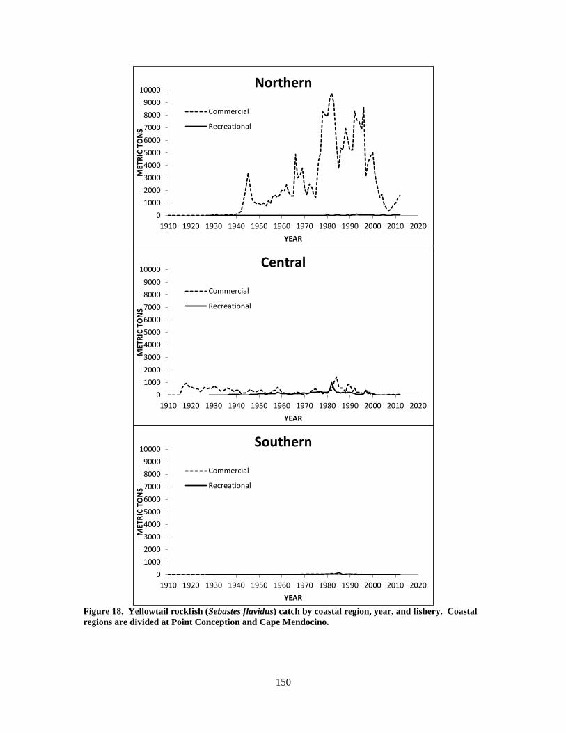
Figure 18. Yellowtail rockfish (Sebastes flavidus) catch by coastal region, year, and fishery. Coastal regions are divided at Point Conception and Cape Mendocino.

0100020003000400050006000700080009000

10000

1910 1920 1930 1940 1950 1960 1970 1980 1990 2000 2010 2020

MET

RIC

TON

S

YEAR

Northern

Commercial

Recreational

0100020003000400050006000700080009000

10000

1910 1920 1930 1940 1950 1960 1970 1980 1990 2000 2010 2020

MET

RIC

TON

S

YEAR

Central

Commercial

Recreational

0100020003000400050006000700080009000

10000

1910 1920 1930 1940 1950 1960 1970 1980 1990 2000 2010 2020

MET

RIC

TON

S

YEAR

Southern

Commercial

Recreational

150

Figure 19. English sole (Parophrys vetulus) commercial landings by coastal region and year. Recreational catch is negligible. Commercial catch reconstructions (data prior to 2007) are from Stewart (2007), whose “Southern” area is equivalent to the Central and Southern areas in this assessment.

0500

100015002000250030003500400045005000

188018901900191019201930194019501960197019801990200020102020

MET

RIC

TON

S

YEAR

Northern

0500

100015002000250030003500400045005000

188018901900191019201930194019501960197019801990200020102020

MET

RIC

TON

S

YEAR

Central & Southern

151

Figure 20. Rex sole (Glyptocephalus zachirus) commercial catch by coastal region and year. Recreational catch is negligible. Coastal regions are divided at Point Conception and Cape Mendocino

0

500

1000

1500

2000

2500

1910 1920 1930 1940 1950 1960 1970 1980 1990 2000 2010 2020

MET

RIC

TON

S

YEAR

Northern

0

500

1000

1500

2000

2500

1910 1920 1930 1940 1950 1960 1970 1980 1990 2000 2010 2020

MET

RIC

TON

S

YEAR

Central

0

500

1000

1500

2000

2500

1910 1920 1930 1940 1950 1960 1970 1980 1990 2000 2010 2020

MET

RIC

TON

S

YEAR

Southern

152

8.1.3 Indices of abundance

Figure 21. Depth and latitudinal occurrence of sharpchin rockfish in each trawl survey by year. Circle size indicates magnitude of catch. Black lines indicate the strata used in the GLMMs. Number in lower right is the percentage of positive tows.

Triennial

Triennial

NWFSC

153

Figure 22. Depth and latitudinal occurrence of stripetail rockfish in each trawl survey by year. Circle size indicates magnitude of catch. Black lines indicate the strata used in the GLMMs. Number in lower right is the percentage of positive tows.

Triennial

Triennial

NWFSC

154

Figure 23. Depth and latitudinal occurrence of yellowtail rockfish (north of 40º10’ N lat.) in each trawl survey by year. Circle size indicates magnitude of catch. Black lines indicate the strata used in the GLMMs. Number in lower right is the percentage of positive tows.

Triennial

Triennial

NWFSC

155

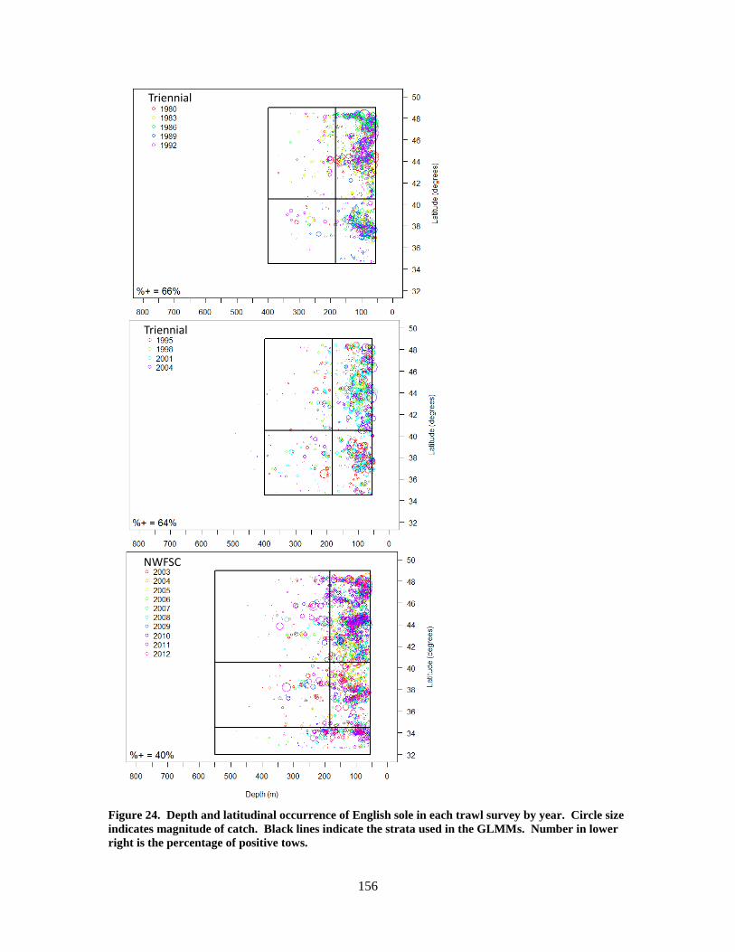
Figure 24. Depth and latitudinal occurrence of English sole in each trawl survey by year. Circle size indicates magnitude of catch. Black lines indicate the strata used in the GLMMs. Number in lower right is the percentage of positive tows.

Triennial

Triennial

NWFSC

156

Figure 25. Depth and latitudinal occurrence of rex sole in each trawl survey by year. Circle size indicates magnitude of catch. Black lines indicate the strata used in the GLMMs. Number in lower right is the percentage of positive tows.

Triennial

Triennial

NWFSC

157

Figure 26. Q-Q plots for the early (1980-1992) AFSC triennial survey series used to diagnose convergence of the Bayesian GLMM model. The yellowtail rockfish (N) plot is for the full time series (1980-2004).

Sharpchin Stripetail Yellowtail North

English sole Rex sole

Uniform

Empi

rical

Empi

rical

158

Figure 27. Q-Q plots for the late (1995-2004) AFSC triennial survey series used to diagnose convergence of the Bayesian GLMM model.

Sharpchin Stripetail


Uniform

Empi

rical

Empi

rical

159

Figure 28. Q-Q plots for the NWFSC annual survey (2003-2012) series used to diagnose convergence of the Bayesian GLMM model.

Sharpchin Stripetail Yellowtail North


Uniform

Empi

rical

Empi

rical

160

Figure 29. Preliminary index of Brown rockfish (S. auriculatus) based on the number of encountered animals; uncertainty based on a jackknife routine.

0

50

100

150

200

250

300

350

1970 1980 1990 2000 2010

"Juvenile" brown rockfish power plant CPUE

161

Figure 30. GLM time series of brown rockfish (central area) abundance indexes from RecFIN sampling. Error bars are 1 standard error from jackknife.

Figure 31. GLM time series of brown rockfish (southern area) abundance indexes from RecFIN sampling. Error bars are 1 standard error from jackknife.

0

0.2

0.4

0.6

0.8

1

1.2

1.4

1.6

1.8

1975 1980 1985 1990 1995 2000 2005

LSM

YEA

R ef

fect

(C p

er a

ngle

r hou

r)

YEAR

0

0.01

0.02

0.03

0.04

0.05

0.06

0.07

0.08

1975 1980 1985 1990 1995 2000 2005

LSM

YEA

R ef

fect

(C p

er a

ngle

r hou

r)

YEAR

162

Figure 32. GLM time series of China rockfish (northern area) abundance indexes from RecFIN sampling. Error bars are 1 standard error from jackknife.

Figure 33. GLM time series of China rockfish (central area) abundance indexes from RecFIN sampling. Error bars are 1 standard error from jackknife.

0

0.02

0.04

0.06

0.08

0.1

0.12

0.14

0.16

0.18

1975 1980 1985 1990 1995 2000 2005

LSM

YEA

R ef

fect

(C p

er a

ngle

r hou

r)

YEAR

0

0.02

0.04

0.06

0.08

0.1

0.12

0.14

1975 1980 1985 1990 1995 2000 2005

LSM

YEA

R ef

fect

(C p

er a

ngle

r hou

r)

YEAR

163

Figure 34. Coefficients (negative, i.e. species that are counter-indicators for copper rockfish in the landed catch) estimated by binomial regression for data filtering for copper rockfish south.

-4 -3.5 -3 -2.5 -2 -1.5 -1 -0.5 0

WBASSCORSQRS

CWCDFNTSSPKL

PBNTBYEL

CMCKCLPR

CUDALngfin Dab

ROCKGBLC

Brd SandbassHNYCCLCOBANK

YLTLGSRK

Blk PerchYCRKYTRKCBZNQFSH

Blk CroakerYTNASTNAALBC

Opaleye

Species Coefficient

164

Figure 35. Coefficients (positive, i.e. species that co-occur with copper rockfish in the landed catch) estimated by binomial regression for data filtering for copper rockfish south.

0 0.2 0.4 0.6 0.8 1

CNRY

BSSH

BGSL

LCOD

GRAS

OLVE

BRWN

TREE

GPHR

Ca Lizardfsh

WDOW

STAR

OWFS

SHPD

Blacksmith

KLBS

JMCK

WCRK

Species Coefficient

165

Figure 36. GLM time series of copper rockfish south abundance indexes from RecFIN sampling. Error bars are 1 standard error from jackknife.

0

0.05

0.1

0.15

0.2

0.25

0.3

1975 1980 1985 1990 1995 2000 2005

LSM

YEA

R ef

fect

(C p

er a

ngle

r hou

r)

YEAR

166

Figure 37. Coefficients estimated by binomial regression for data filtering copper rockfish north/central area.

-3 -2.5 -2 -1.5 -1 -0.5 0 0.5 1

FLAGBRWN

ROSYVRMLCWCDQLBKKLPR

SWSPCNRYGPHRPDABTIGRKLPGBLURCBZNBCACSSOLSTAR

CHNALCODGSPTOLVEYTRKTREESQRSCHLBPTRLREDSRSOLJMCKYEYEBLCK

WDOWSABLPHLB

CMCKRSTN

COHOSLGRSPKL

GSRKCLPR

ROCKCHNKPWHT

BYELALBCSTBS

Species Coefficient

167

Figure 38. GLM time series of copper rockfish (north/central) abundance indexes from RecFIN sampling. Error bars are 1 standard error from jackknife.

0

0.02

0.04

0.06

0.08

0.1

0.12

0.14

0.16

0.18

0.2

1975 1980 1985 1990 1995 2000 2005

LSM

YEA

R ef

fect

(C p

er a

ngle

r hou

r)

YEAR

168

Figure 39. Year effects and 95% lognormal confidence intervals from the Central California onboard CPFV observer index for brown rockfish.

Figure 40. Comparison of area-weighted and “main effects” abundance indices for China rockfish in central California, estimated from onboard CPFV observer data.

0

0.2

0.4

0.6

0.8

1

1.2

1986 1988 1990 1992 1994 1996 1998 2000 2002 2004 2006 2008 2010 2012

INDE

X

YEAR

0

0.01

0.02

0.03

0.04

0.05

0.06

0.07

0.08

0.09

0.1

1985 1990 1995 2000 2005 2010 2015

INDE

X

YEAR

Area-Weighted (AIC best)

Main Effects (BIC best)

169

Figure 41. Year effects and 95% lognormal confidence intervals from the Central California onboard CPFV observer index for China rockfish.

Figure 42. Year effects and 95% lognormal confidence intervals from the Central California onboard CPFV observer index for copper rockfish.

0

0.02

0.04

0.06

0.08

0.1

0.12

0.14

0.16

0.18

0.2

1985 1990 1995 2000 2005 2010 2015

INDE

X

0

0.05

0.1

0.15

0.2

0.25

1985 1990 1995 2000 2005 2010 2015

INDE

X

170

Figure 43. Year effects from the Central California onboard CPFV observer index for copper rockfish, with a comparison of indices derived using data from all regulatory periods (“all regs included”) and data excluding locations and time periods with 20-fathom depth restrictions (“No 20-fm obs”).

0

0.02

0.04

0.06

0.08

0.1

0.12

0.14

0.16

0.18

1985 1990 1995 2000 2005 2010 2015

No 20-fm obs

all regs included

171

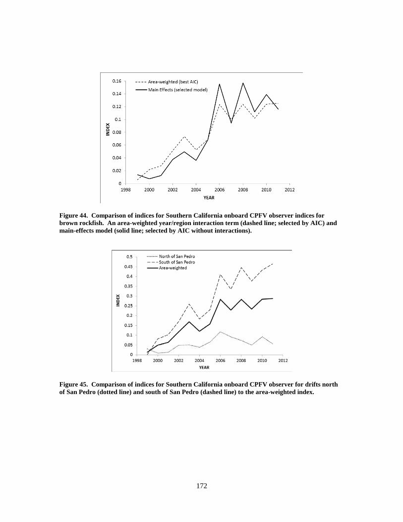
Figure 44. Comparison of indices for Southern California onboard CPFV observer indices for brown rockfish. An area-weighted year/region interaction term (dashed line; selected by AIC) and main-effects model (solid line; selected by AIC without interactions).

Figure 45. Comparison of indices for Southern California onboard CPFV observer for drifts north of San Pedro (dotted line) and south of San Pedro (dashed line) to the area-weighted index.

172

Figure 46. Year effects and 95% lognormal confidence intervals from the Southern California onboard CPFV observer index for brown rockfish.

Figure 47. Comparison of indices for Southern California onboard CPFV observer indices for copper rockfish. An area-weighted year/region interaction term (dashed line; selected by AIC) and main-effects model (solid line; selected by BIC without interactions).

173

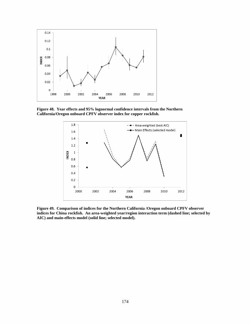
Figure 48. Year effects and 95% lognormal confidence intervals from the Northern California/Oregon onboard CPFV observer index for copper rockfish.

Figure 49. Comparison of indices for the Northern California /Oregon onboard CPFV observer indices for China rockfish. An area-weighted year/region interaction term (dashed line; selected by AIC) and main-effects model (solid line; selected model).

174

Figure 50. Year effects and 95% lognormal confidence intervals from the Northern California/Oregon onboard CPFV observer index for China rockfish.

175

Figure 51. Comparison of indices for the Northern California /Oregon onboard CPFV observer indices for copper rockfish. An area-weighted year/region interaction term (dashed line; selected by AIC) and main-effects model (solid line; selected model).

Figure 52. Year effects and 95% lognormal confidence intervals from the Northern California/Oregon onboard CPFV observer index for copper rockfish.

176

Figure 53. The relationship between relative abundance in 2000 (B2000/Bunfished) and a PSA vulnerability score reflecting pre-2000 fishery management.

Figure 54. Prior distributions for alternative vulnerability scores.

0

0.2

0.4

0.6

0.8

1

1.2

1.4

1 1.2 1.4 1.6 1.8 2 2.2 2.4 2.6 2.8

Rela

tive

Abun

danc

e in

200

0

Vulnerability Score pre-2000

0

0.05

0.1

0.15

0.2

0 0.2 0.4 0.6 0.8 1

Dens

ity

Relative Abundance in 2000

Middle V (mean 0.3, SD 0.2)

Uninformative (mean 0.4, SD 0.3)

Low V (mean 0.65, SD 0.2)

177

8.2 Model Results and Diagnostic Figures 8.2.1 Brown rockfish

Figure 55. XDB-SRA results for brown rockfish. Upper left: bivariate prior and posterior distributions for FMSY/M and BMSY/B0. Red lines are 75% and 95% contours of the prior, blue lines are updated posterior contours. Grey circles are posterior draws, large solid circles are centroids (medians) of the prior and posterior (red and blue, respectively). Upper right: trends in relative exploitation rate and relative biomass. Horizontal solid line is target exploitation rate (model-estimated), vertical lines (dashed and dotted) are target and threshold biomass values, 0.4B0 and 0.25B0, respectively. Lower left: Median, 5% and 95% quantiles of spawning biomass relative to target and minimum stock size threshold (MSST). Lower right: posterior density of current depletion (biomass in 2013 relative to unfished biomass).

178

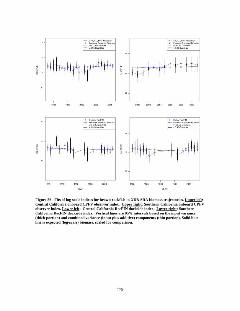
Figure 56. Fits of log-scale indices for brown rockfish to XDB-SRA biomass trajectories. Upper left: Central California onboard CPFV observer index. Upper right: Southern California onboard CPFV observer index. Lower left: Central California RecFIN dockside index. Lower right: Southern California RecFIN dockside index. Vertical lines are 95% intervals based on the input variance (thick portion) and combined variance (input plus additive) components (thin portion). Solid blue line is expected (log-scale) biomass, scaled for comparison.

179

Figure 57. XDB-SRA results for brown rockfish (coastwide). Top panel: indices of abundance rescaled into biomass units (see previous figure for index descriptions). Bottom panels: prior (dotted), post-model pre-data (dashed), and posterior (solid) distributions of XDB-SRA population dynamics parameters.

180

8.2.2 China rockfish 8.2.2.1 Central and Southern California

Figure 58. XDB-SRA results for China rockfish (south of 40° 10′ N lat.). Upper left: bivariate prior and posterior distributions for FMSY/M and BMSY/B0. Red lines are 75% and 95% contours of the prior, blue lines are updated posterior contours. Grey circles are posterior draws, black circles represent rejected runs (biomass <0), large solid circles are centroids (medians) of the prior and posterior (red and blue, respectively). Upper right: trends in relative exploitation rate and relative biomass. Horizontal solid line is target exploitation rate (model-estimated), vertical lines (dashed and dotted) are target and threshold biomass values, 0.4B0 and 0.25B0, respectively. Lower left: Median, 5% and 95% quantiles of spawning biomass relative to target and minimum stock size threshold (MSST). Lower right: posterior density of current depletion (biomass in 2013 relative to unfished biomass).

181

Figure 59. Fits of log-scale indices to XDB-SRA biomass trajectories for China rockfish (south of 40° 10′ N lat.). Left: Central California RecFIN dockside index. Right: Central California onboard CPFV observer index. Vertical lines are 95% intervals based on the input variance (thick portion) and combined variance (input plus additive) components (thin portion). Solid blue line is expected log-scale biomass, scaled for comparison.

182

Figure 60. XDB-SRA results for China rockfish (south of 40° 10′ N lat.). Top panel: indices of abundance rescaled into biomass units (see previous figure for index descriptions). Bottom panels: prior (dotted), post-model pre-data (dashed), and posterior (solid) distributions of XDB-SRA parameters.

183

8.2.2.2 Northern China Rockfish (N of 40° 10′ N lat.).

Figure 61. XDB-SRA results for China rockfish (north of 40° 10′ N lat.). Upper left: bivariate prior and posterior distributions for FMSY/M and BMSY/B0. Red lines are 75% and 95% contours of the prior, blue lines are updated posterior contours. Grey circles are posterior draws, black circles represent rejected runs (biomass <0), large solid circles are centroids (medians) of the prior and posterior (red and blue, respectively). Upper right: trends in relative exploitation rate and relative biomass. Horizontal solid line is target exploitation rate (model-estimated), vertical lines (dashed and dotted) are target and threshold biomass values, 0.4B0 and 0.25B0, respectively. Lower left: Median, 5% and 95% quantiles of spawning biomass relative to target and minimum stock size threshold (MSST). Lower right: posterior density of current depletion (biomass in 2013 relative to unfished biomass).

184

Figure 62. Fits of log-scale indices to XDB-SRA biomass trajectories for China rockfish (north of 40° 10′ N lat.). Left: No. CA / OR RecFIN dockside index. Right: Oregon onboard CPFV observer index. Vertical lines are 95% intervals based on the input variance (thick portion) and combined variance (input plus additive) components (thin portion). Solid blue line is expected log-scale biomass, scaled for comparison.

185

Figure 63. XDB-SRA results for China rockfish (north of 40° 10′ N lat.). Top panel: indices of abundance rescaled into biomass units (see previous figure for index descriptions). Bottom panels: prior (dotted), post-model pre-data (dashed), and posterior (solid) distributions of XDB-SRA parameters.

186

8.2.3 Copper rockfish 8.2.3.1 Copper Rockfish North of Point Conception (34° 27′ N lat.)

Figure 64. XDB-SRA results for copper rockfish (north of 34° 27′ N lat.). Upper left: bivariate prior and posterior distributions for FMSY/M and BMSY/B0. Red lines are 75% and 95% contours of the prior, blue lines are updated posterior contours. Grey circles are posterior draws, black circles represent rejected runs (biomass <0), large solid circles are centroids (medians) of the prior and posterior (red and blue, respectively). Upper right: trends in relative exploitation rate and relative biomass. Horizontal solid line is target exploitation rate (model-estimated), vertical lines (dashed and dotted) are target and threshold biomass values, 0.4B0 and 0.25B0, respectively. Lower left: Median, 5% and 95% quantiles of spawning biomass relative to target and minimum stock size threshold (MSST). Lower right: posterior density of current depletion (biomass in 2013 relative to unfished biomass).

187

Figure 65. Fits of log-scale indices to XDB-SRA biomass trajectories for copper rockfish (north of 34° 27′ N lat.). Upper left: Central California onboard CPFV observer index. Upper right: Central/Northern California and Oregon RecFIN dockside index. Lower left: Oregon onboard CPFV observer index. Vertical lines are 95% intervals based on the input variance (thick portion) and combined variance (input plus additive) components (thin portion). Solid blue line is expected log-scale biomass, scaled for comparison.

188

Figure 66. XDB-SRA results for copper rockfish (north of 34° 27′ N lat.). Top panel: indices of abundance rescaled into biomass units (see previous figure for index descriptions). Bottom panels: prior (dotted), post-model pre-data (dashed), and posterior (solid) distributions of XDB-SRA parameters.

189

8.2.3.2 Southern Copper Rockfish (S. of 34° 27′ N lat.).

Figure 67. XDB-SRA results for copper rockfish (south of 34° 27′ N lat.). Upper left: bivariate prior and posterior distributions for FMSY/M and BMSY/B0. Red lines are 75% and 95% contours of the prior, blue lines are updated posterior contours. Grey circles are posterior draws, black circles represent rejected runs (biomass <0), large solid circles are centroids (medians) of the prior and posterior (red and blue, respectively). Upper right: trends in relative exploitation rate and relative biomass. Horizontal solid line is target exploitation rate (model-estimated), vertical lines (dashed and dotted) are target and threshold biomass values, 0.4B0 and 0.25B0, respectively. Lower left: Median, 5% and 95% quantiles of spawning biomass relative to target and minimum stock size threshold (MSST). Lower right: posterior density of current depletion (biomass in 2013 relative to unfished biomass).

190

Figure 68. Fits of log-scale indices to XDB-SRA biomass trajectories for copper rockfish (south of 34° 27′ N lat.). Index 1: Southern California onboard CPFV observer index. Index 2: Southern California RecFIN dockside index. Vertical lines are 95% intervals based on the input variance (thick portion) and combined variance (input plus additive) components (thin portion). Solid blue line is expected log-scale biomass.

191

Figure 69. XDB-SRA results for copper rockfish (south of 34° 27′ N lat.). Top panel: indices of abundance rescaled into biomass units (see previous figure for index descriptions). Bottom panels: prior (dotted), post-model pre-data (dashed), and posterior (solid) distributions of XDB-SRA parameters.

192

8.2.4 Sharpchin rockfish

Figure 70. Fits to the three fishery-independent surveys from the exSSS model for sharpchin rockfish. Thick lines are inputted variance; thin lines are estimated added variance.

193

Figure 71. Posterior distribution of the catchability parameters (q) for each index fit in the exSSS AIS sharpchin rockfish assessment. Vertical line indicate q=1.

194

Figure 72. Entropy and model weight values used to determine model convergence in the exSSS AIS models for 4 stocks. Dotted horizontal line is the threshold entropy value of 0.92 indicating convergence.

195

Figure 73. Prior and posterior distributions for each input parameter of the exSSS AIS uncertainty estimation for sharpchin rockfish.

196

Figure 74. Pairs plots for each parameter in the exSSS AIS treatment of uncertainty for sharpchin rockfish.

197

Figure 75. Time series of spawning biomass from the exSSS MLE (broken line) and AIS (solid line with gray uncertainty bars) for sharpchin rockfish. Catch history is provided below the 0 line.

198

Figure 76. Time series of stock status (depletion) from the exSSS MLE (broken line) and AIS (solid line with gray uncertainty bars) for sharpchin rockfish.

199

Figure 77. Stock status posterior distribution from the exSSS AIS model for sharpchin rockfish.

200

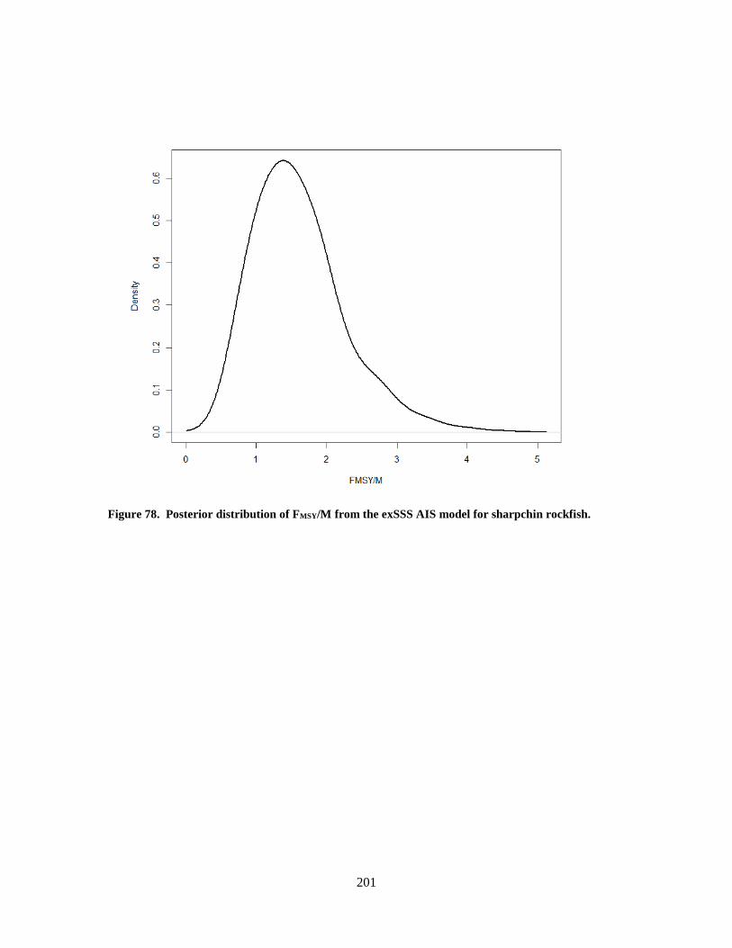
Figure 78. Posterior distribution of FMSY/M from the exSSS AIS model for sharpchin rockfish.

201

Figure 79. Posterior distribution of OFLs from the exSSS AIS model for sharpchin rockfish.

202

Figure 80 . Comparison of the exSSS AIS (black line, gray shaded 95% CI) and catch-only (SSS; red broken line; pink shaded 95% CI) estimates of spawning biomass (upper panel) and stock status (lower panel) for sharpchin rockfish. Darker red shaded area is the overlap of the top models.

203

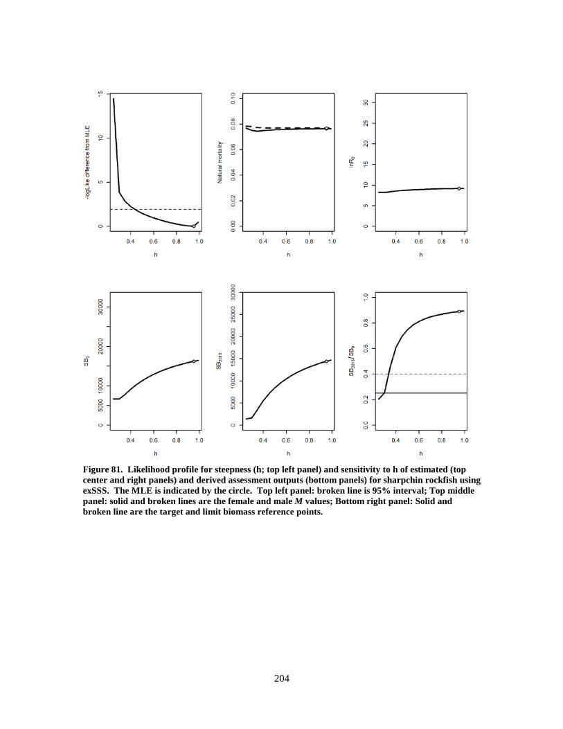
Figure 81. Likelihood profile for steepness (h; top left panel) and sensitivity to h of estimated (top center and right panels) and derived assessment outputs (bottom panels) for sharpchin rockfish using exSSS. The MLE is indicated by the circle. Top left panel: broken line is 95% interval; Top middle panel: solid and broken lines are the female and male M values; Bottom right panel: Solid and broken line are the target and limit biomass reference points.

204

Figure 82. Steepness profile relative to XDB-SRA productivity parameters FMSY/M (top panel) and BMSY/B0 (bottom panel) for sharpchin rockfish. Circle indicates exSSS MLE estimate. Broken line is the prior mean used in XDB-SRA.

205

8.2.5 Yellowtail rockfish (North of 40° 10’ N lat.)

Figure 83. Fits to the three fishery-independent surveys from the exSSS AIS model for yellowtail rockfish (North of 40° 10’ N lat.). Thick lines are inputted variance; thin lines are estimated added variance.

206

Figure 84. Posterior distribution of the added variance for each index fit in the exSSS AIS yellowtail rockfish (North of 40° 10’ N lat.) assessment.

207

Figure 85. Posterior distribution of the catchability parameters (q) for each index fit in the exSSS AIS yellowtail rockfish (North of 40° 10’ N lat.) assessment.

208

Figure 86. Prior and posterior distributions for each input parameter of the exSSS AIS uncertainty estimation for yellowtail rockfish (North of 40° 10’ N lat.).

209

Figure 87. Pairs plots for each parameter in the exSSS AIS treatment of uncertainty for yellowtail rockfish (North of 40° 10’ N lat.).

210

Figure 88. Time series of spawning biomass from the exSSS MLE (broken line) and AIS (solid line with gray uncertainty bars) for yellowtail rockfish (North of 40° 10’ N lat.). Catch history is provided below the 0 line.

211

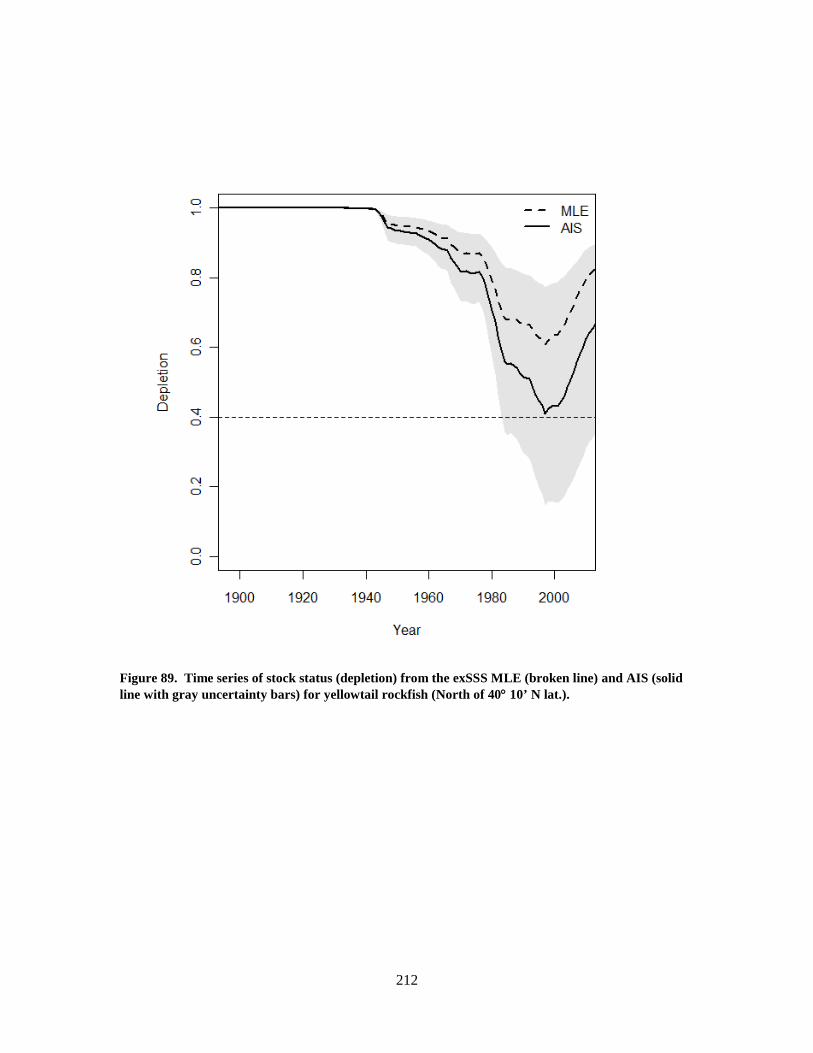
Figure 89. Time series of stock status (depletion) from the exSSS MLE (broken line) and AIS (solid line with gray uncertainty bars) for yellowtail rockfish (North of 40° 10’ N lat.).

212

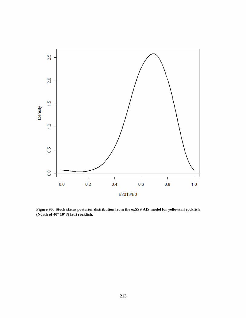
Figure 90. Stock status posterior distribution from the exSSS AIS model for yellowtail rockfish (North of 40° 10’ N lat.) rockfish.

213

Figure 91. Comparison of exSSS estimated spawning biomass (black line with gray shading indicating the 95% CI) to past stock assessments of the yellowtail rockfish (North of 40° 10’ N lat.).

214

Figure 92. Posterior distribution of FMSY/M from the exSSS AIS model for yellowtail rockfish (North of 40° 10’ N lat.).

215

Figure 93. Posterior distribution of OFLs from the exSSS AIS model for yellowtail rockfish (North of 40° 10’ N lat.).

216

Figure 94. Comparison of the exSSS AIS (black line, gray shaded 95% CI) and catch-only (SSS; red broken line; pink shaded 95% CI) estimates of spawning biomass (upper panel) and stock status (lower panel) for yellowtail rockfish (North of 40° 10’ N lat.). Darker red shaded area is the overlap of the top models.

217

Figure 95. Likelihood profile for steepness (h; top left panel) and sensitivity to h of estimated (top center and right panels) and derived assessment outputs (bottom panels) for yellowtail rockfish (North of 40° 10’ N lat.) using exSSS. The MLE is indicated by the circle. Top left panel: broken line is 95% interval; Top middle panel: solid and broken lines are the female and male M values; Bottom right panel: Solid and broken line are the target and limit biomass reference points.

218

Figure 96. Steepness profile relative to XDB-SRA productivity parameters FMSY/M (top panel) and BMSY/B0 (bottom panel) for yellowtail rockfish (North of 40° 10’ N lat.). Circle indicates exSSS MLE estimate. Broken line is the prior mean used in XDB-SRA.

219

8.2.6 English sole

Figure 97. Fits to the three fishery-independent surveys from the exSSS AIS model for English sole. Thick lines are inputted variance; thin lines are estimated added variance.

220

Figure 98. Posterior distribution of the added variance for each index fit in the exSSS AIS English sole assessment.

221

Figure 99. Posterior distribution of the catchability parameters (q) for each index fit in the exSSS AIS English sole assessment. Vertical line indicates q=1.

222

Figure 100. Prior and posterior distributions for each input parameter of the exSSS AIS uncertainty estimation for English sole.

223

Figure 101. Pairs plots for each parameter in the exSSS AIS treatment of uncertainty for English sole.

224

Figure 102. Time series of spawning biomass from the exSSS MLE (broken line) and AIS (solid line with gray uncertainty bars) for English sole. Catch history is provided below the 0 line.

225

Figure 103. Time series of stock status (depletion) from the exSSS MLE (broken line) and AIS (solid line with gray uncertainty bars) for English sole.

226

Figure 104. Stock status posterior distribution from the exSSS AIS model for English sole.

227

Figure 105. Comparison of the exSSS model (black line with gray shading of 95% CI) to the 2009 full assessment (red broken line with red shading of 95% CI) of English sole.

228

Figure 106. Posterior distribution of FMSY/M from the exSSS AIS model for English sole.

229

Figure 107. Posterior distribution of OFLs from the exSSS AIS model for English sole.

230

Figure 108. Comparison of the exSSS AIS (black line, gray shaded 95% CI) and catch-only (SSS; red broken line; pink shaded 95% CI) estimates of spawning biomass (upper panel) and stock status (lower panel) for English sole. Darker red shaded area is the overlap of the top models.

231

Figure 109. Likelihood profile for steepness (h; top left panel) and sensitivity to h of estimated (top center and right panels) and derived assessment outputs (bottom panels) for English sole using exSSS. The MLE is indicated by the circle. Top left panel: broken line is 95% interval; Top middle panel: solid and broken lines are the female and male M values; Bottom right panel: Solid and broken line are the target and limit biomass reference points.

232

Figure 110. Steepness profile relative to XDB-SRA productivity parameters FMSY/M (top panel) and BMSY/B0 (bottom panel) for English sole. Circle indicates exSSS MLE estimate. Broken line is the prior mean used in XDB-SRA.

233

8.2.7 Rex sole

Figure 111. Fits to the three fishery-independent surveys from the exSSS AIS model for rex sole. Thick lines are inputted variance; thin lines are estimated added variance.

234

Figure 112. Posterior distribution of the added variance for each index fit in the exSSS AIS rex sole assessment.

235

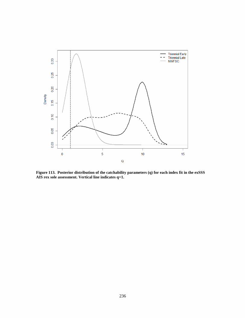
Figure 113. Posterior distribution of the catchability parameters (q) for each index fit in the exSSS AIS rex sole assessment. Vertical line indicates q=1.

236

Figure 114. Prior and posterior distributions for each input parameter of the exSSS AIS uncertainty estimation for rex sole.

237

Figure 115. Pairs plots for each parameter in the exSSS AIS treatment of uncertainty for rex sole.

238

Figure 116. Time series of spawning biomass from the exSSS MLE (broken line) and AIS (solid line with gray uncertainty bars) for rex sole. Catch history is provided below the 0 line.

239

Figure 117. Time series of stock status (depletion) from the exSSS MLE (broken line) and AIS (solid line with gray uncertainty bars) for rex sole.

240

Figure 118. Stock status posterior distribution from the exSSS AIS model for rex sole.

241

Figure 119. Posterior distribution of FMSY/M from the exSSS AIS model for rex sole.

242

Figure 120. Posterior distribution of OFLs from the exSSS AIS model for rex sole.

243

Figure 121. Comparison of the exSSS AIS (black line, gray shaded 95% CI) and catch-only (SSS; red broken line; pink shaded 95% CI) estimates of spawning biomass (upper panel) and stock status (lower panel) for rex sole. Darker red shaded area is the overlap of the top models.

244

Figure 122. Likelihood profile for steepness (h; top left panel) and sensitivity to h of estimated (top center and right panels) and derived assessment outputs (bottom panels) for rex sole using exSSS. The MLE is indicated by the circle. Top left panel: broken line is 95% interval; Top middle panel: solid and broken lines are the female and male M values; Bottom right panel: Solid and broken line are the target and limit biomass reference points.

245

Figure 123. Steepness profile relative to XDB-SRA productivity parameters FMSY/M (top panel) and BMSY/B0 (bottom panel) for rex sole. Circle indicates exSSS MLE estimate. Broken line is the prior mean used in XDB-SRA.

246

8.2.8 Stripetail rockfish

Figure 124. Likelihood, parameter (h), and derived outputs (depletion and OFL2015) profiles over the log of initial recruitment (lnR0) for the stripetail rockfish.

247

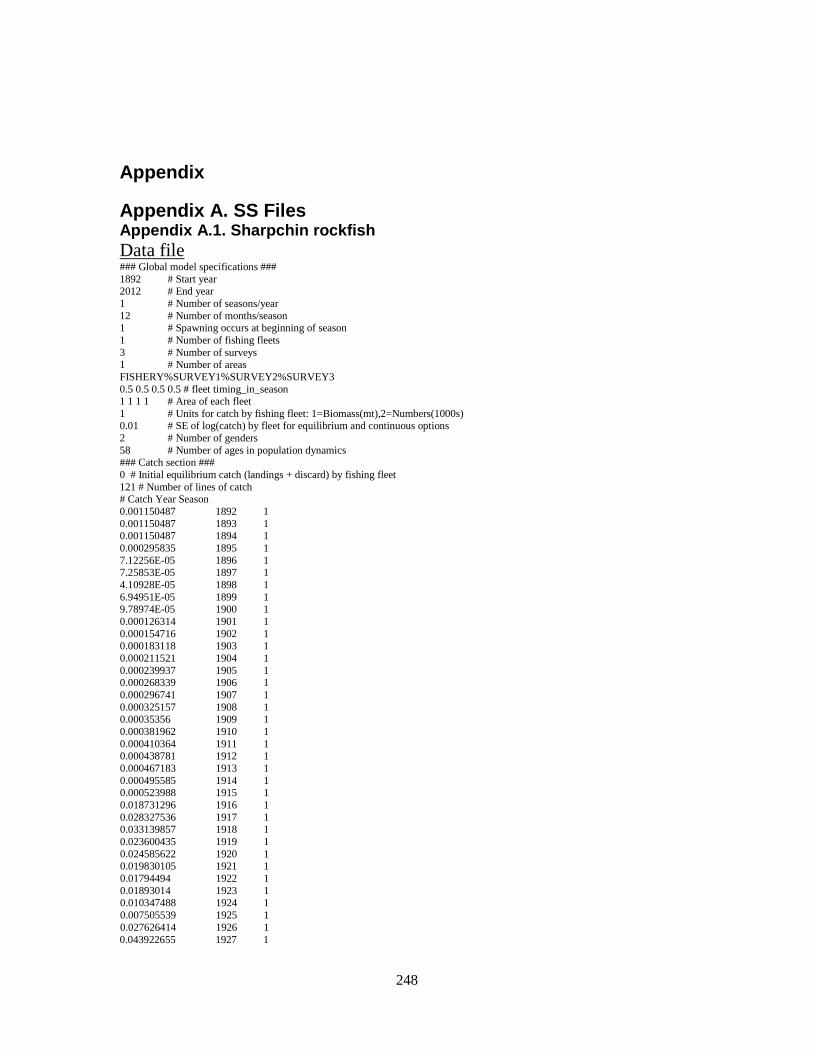
Appendix Appendix A. SS Files Appendix A.1. Sharpchin rockfish Data file ### Global model specifications ### 1892 # Start year 2012 # End year 1 # Number of seasons/year 12 # Number of months/season 1 # Spawning occurs at beginning of season 1 # Number of fishing fleets 3 # Number of surveys 1 # Number of areas FISHERY%SURVEY1%SURVEY2%SURVEY3 0.5 0.5 0.5 0.5 # fleet timing_in_season 1 1 1 1 # Area of each fleet 1 # Units for catch by fishing fleet: 1=Biomass(mt),2=Numbers(1000s) 0.01 # SE of log(catch) by fleet for equilibrium and continuous options 2 # Number of genders 58 # Number of ages in population dynamics ### Catch section ### 0 # Initial equilibrium catch (landings + discard) by fishing fleet 121 # Number of lines of catch # Catch Year Season 0.001150487 1892 1 0.001150487 1893 1 0.001150487 1894 1 0.000295835 1895 1 7.12256E-05 1896 1 7.25853E-05 1897 1 4.10928E-05 1898 1 6.94951E-05 1899 1 9.78974E-05 1900 1 0.000126314 1901 1 0.000154716 1902 1 0.000183118 1903 1 0.000211521 1904 1 0.000239937 1905 1 0.000268339 1906 1 0.000296741 1907 1 0.000325157 1908 1 0.00035356 1909 1 0.000381962 1910 1 0.000410364 1911 1 0.000438781 1912 1 0.000467183 1913 1 0.000495585 1914 1 0.000523988 1915 1 0.018731296 1916 1 0.028327536 1917 1 0.033139857 1918 1 0.023600435 1919 1 0.024585622 1920 1 0.019830105 1921 1 0.01794494 1922 1 0.01893014 1923 1 0.010347488 1924 1 0.007505539 1925 1 0.027626414 1926 1 0.043922655 1927 1

248

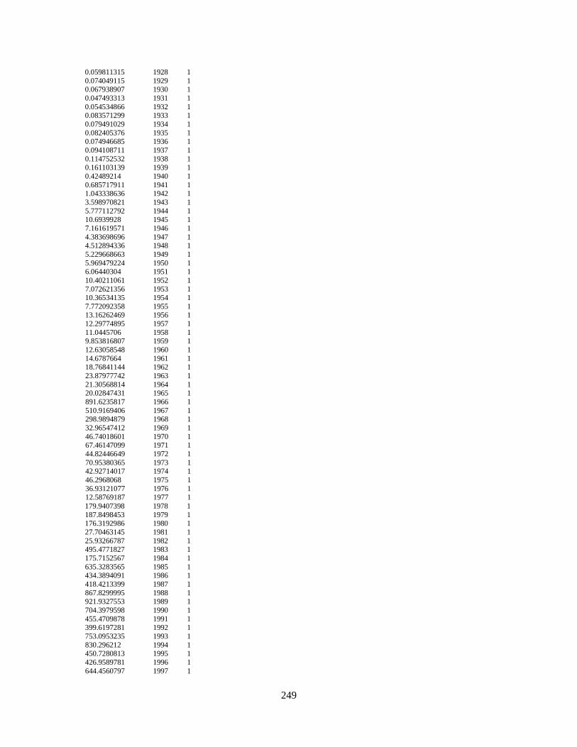
0.059811315 1928 1 0.074049115 1929 1 0.067938907 1930 1 0.047493313 1931 1 0.054534866 1932 1 0.083571299 1933 1 0.079491029 1934 1 0.082405376 1935 1 0.074946685 1936 1 0.094108711 1937 1 0.114752532 1938 1 0.161103139 1939 1 0.42489214 1940 1 0.685717911 1941 1 1.043338636 1942 1 3.598970821 1943 1 5.777112792 1944 1 10.6939928 1945 1 7.161619571 1946 1 4.383698696 1947 1 4.512894336 1948 1 5.229668663 1949 1 5.969479224 1950 1 6.06440304 1951 1 10.40211061 1952 1 7.072621356 1953 1 10.36534135 1954 1 7.772092358 1955 1 13.16262469 1956 1 12.29774895 1957 1 11.0445706 1958 1 9.853816807 1959 1 12.63058548 1960 1 14.6787664 1961 1 18.76841144 1962 1 23.87977742 1963 1 21.30568814 1964 1 20.02847431 1965 1 891.6235817 1966 1 510.9169406 1967 1 298.9894879 1968 1 32.96547412 1969 1 46.74018601 1970 1 67.46147099 1971 1 44.82446649 1972 1 70.95380365 1973 1 42.92714017 1974 1 46.2968068 1975 1 36.93121077 1976 1 12.58769187 1977 1 179.9407398 1978 1 187.8498453 1979 1 176.3192986 1980 1 27.70463145 1981 1 25.93266787 1982 1 495.4771827 1983 1 175.7152567 1984 1 635.3283565 1985 1 434.3894091 1986 1 418.4213399 1987 1 867.8299995 1988 1 921.9327553 1989 1 704.3979598 1990 1 455.4709878 1991 1 399.6197281 1992 1 753.0953235 1993 1 830.296212 1994 1 450.7280813 1995 1 426.9589781 1996 1 644.4560797 1997 1

249

199.629736 1998 1 93.84972025 1999 1 18.17774475 2000 1 13.52855594 2001 1 9.518229623 2002 1 8.005632828 2003 1 38.17946805 2004 1 5.748690254 2005 1 0.255711987 2006 1 3.842639735 2007 1 1.839040923 2008 1 2.037965884 2009 1 0.569843338 2010 1 0.783928411 2011 1 13.68731875 2012 1 19 # Number of index observations # Units: 0=numbers,1=biomass,2=F; Errortype: -1=normal,0=lognormal,>0=T # Fleet Units Errortype 1 1 0 # fleet 1: FISHERY 2 1 0 # fleet 2: SURVEY 3 1 0 # fleet 2: SURVEY 4 1 0 # fleet 2: SURVEY #_year seas index obs se(log) 1980 1 2 12581.44 0.462964486 #Tri early 1983 1 2 16110.57 0.374595369 1986 1 2 8634.25 0.580113613 1989 1 2 9519.64 .383331259 1992 1 2 9108.24 0.391341879 1995 1 3 3938.93 0.466238502 #Tri late 1998 1 3 2202.63 0.454324983 2001 1 3 1661.22 0.469075594 2004 1 3 4134.65 0.443822656 2003 1 4 50174.25399 0.471483982 #NWFSC 2004 1 4 117780.528 0.588720526 2005 1 4 68461.82512 0.489966596 2006 1 4 43764.76248 0.539389308 2007 1 4 32385.21202 0.534870966 2008 1 4 36878.05159 0.529974414 2009 1 4 49675.6004 0.464195841 2010 1 4 29165.19996 0.418899015 2011 1 4 53769.16783 0.463277617 2012 1 4 41190.7276 0.457001953 0 #_N_fleets_with_discard 0 #_N_discard_obs 0 #_N_meanbodywt_obs 30 #_DF_meanwt ## Population size structure 1 # length bin method: 1=use databins; 2=generate from binwidth,min,max below; 3=read vector # binwidth for population size comp # minimum size in the population (lower edge of first bin and size at age 0.00) # maximum size in the population (lower edge of last bin) -1 #_comp_tail_compression 1e-007 #_add_to_comp 0 #_combine males into females at or below this bin number 22 #_N_LengthBins 2 4 6 8 10 12 14 16 18 20 22 24 26 28 30 32 34 36 38 40 42 44 0 #_N_Length_obs #Yr Seas Flt/Svy Gender Part Nsamp datavector(female-male) 52 #_N_age_bins 1 2 3 4 5 6 7 8 9 10 11 12 13 14 15 16 17 18 19 20 21 22 23 24 25 26 27 28 29 30 31 32 33 34 35 36 37 38 39 40 41 42 43 44 45 46 47 48 49 50 51 52 0 #_N_ageerror_definitions 0 #_N_Agecomp_obs 1 #_Lbin_method: 1=poplenbins; 2=datalenbins; 3=lengths

250

0 #_combine males into females at or below this bin number 0 #_N_MeanSize-at-Age_obs 0 #_N_environ_variables 0 #_N_environ_obs 0 # N sizefreq methods to read 0 # no tag data 0 # no morphcomp data 999 # End data file Control file #C growth parameters are estimated 1 #_N_Growth_Patterns 1 #_N_Morphs_Within_GrowthPattern 0 #_Nblock_Patterns #_Cond 0 #_blocks_per_pattern 0.5 #_fracfemale 0 #_natM_type:_0=1Parm; 1=N_breakpoints;_2=Lorenzen;_3=agespecific;_4=agespec_withseasinterpolate #_no additional input for selected M option; read 1P per morph 1 # GrowthModel: 1=vonBert with L1andL2; 2=Richards with L1andL2; 3=not implemented; 4=not implemented 1 #_Growth_Age_for_L1 999 #_Growth_Age_for_L2 (999 to use as Linf) 0 #_SD_add_to_LAA (set to 0.1 for SS2 V1.x compatibility) 0 #_CV_Growth_Pattern: 0 CV=f(LAA); 1 CV=F(A); 2 SD=F(LAA); 3 SD=F(A) 1 #_maturity_option: 1=length logistic; 2=age logistic; 3=read age-maturity matrix by growth_pattern; 4=read age-fecundity; 5=read fec and wt from wtatage.ss #_placeholder for empirical age-maturity by growth pattern 0 #_First_Mature_Age 1 #_fecundity option:(1)eggs=Wt*(a+b*Wt);(2)eggs=a*L^b;(3)eggs=a*Wt^b 0 #_hermaphroditism option: 0=none; 1=age-specific fxn 1 #_parameter_offset_approach (1=none, 2= M, G, CV_G as offset from female-GP1, 3=like SS2 V1.x) 2 #_env/block/dev_adjust_method (1=standard; 2=logistic transform keeps in base parm bounds; 3=standard w/ no bound check) # #_growth_parms #_LO HI INIT PRIOR PR_type SD PHASE env-var use_dev dev_minyr dev_maxyr dev_stddev Block Block_Fxn 0.001 2 0.077 -2.564 3 0.4 2 0 0 0 0 0 0 0 # NatM_p_1_Fem_GP_1 1 16.50117351 8.250586756 36 -1 10 -2 0 0 0 0 0 0 0 # L_at_Amin_Fem_GP_1 1 66.42 33.21 70 -1 10 -4 0 0 0 0 0 0 0 # L_at_Amax_Fem_GP_1 0.05 0.34 0.17 0.15 -1 0.8 -4 0 0 0 0 0 0 0 # VonBert_K_Fem_GP_1 0.05 0.2 0.1 0.1 -1 0.8 -3 0 0 0 0 0 0 0 # CV_young_Fem_GP_1 0.05 0.2 0.1 0.1 -1 0.8 -3 0 0 0 0 0 0 0 # CV_old_Fem_GP_1 0.001 2 0.077 -2.564 3 0.4 2 0 0 0 0 0 0 0 # NatM_p_1_Fem_GP_1 1 16.50117351 8.23 36 -1 10 -2 0 0 0 0 0 0 0 # L_at_Amin_Fem_GP_1 1 66.42 26.98 70 -1 10 -4 0 0 0 0 0 0 0 # L_at_Amax_Fem_GP_1 0.05 0.34 0.2 0.15 -1 0.8 -4 0 0 0 0 0 0 0 # VonBert_K_Fem_GP_1 0.05 0.2 0.1 0.1 -1 0.8 -3 0 0 0 0 0 0 0 # CV_young_Fem_GP_1 0.05 0.2 0.1 0.1 -1 0.8 -3 0 0 0 0 0 0 0 # CV_old_Fem_GP_1 -3 3 8.27E-06 2.44E-06 -1 0.8 -3 0 0 0 0 0 0 0 # Wtlen_1_Fem -3 4 3.16 3.34694 -1 0.8 -3 0 0 0 0 0 0 0 # Wtlen_2_Fem 1 1000 22 55 -1 0.8 -3 0 0 0 0 0 0 0 # Mat50%_Fem -3 3 -5.01 -0.25 -1 0.8 -3 0 0 0 0 0 0 0 # Mat_slope_Fem -3 3 1 1 -1 0.8 -3 0 0 0 0 0 0 0 # Eggs/kg_inter_Fem -3 3 0 0 -1 0.8 -3 0 0 0 0 0 0 0 # Eggs/kg_slope_wt_Fem -3 3 9.10E-06 2.44E-06 -1 0.8 -3 0 0 0 0 0 0 0 # Wtlen_1_Mal -3 4 3.13 3.34694 -1 0.8 -3 0 0 0 0 0 0 0 # Wtlen_2_Mal

251

0 0 0 0 -1 0 -4 0 0 0 0 0 0 0 # RecrDist_GP_1 0 0 0 0 -1 0 -4 0 0 0 0 0 0 0 # RecrDist_Area_1 0 0 0 0 -1 0 -4 0 0 0 0 0 0 0 # RecrDist_Seas_1 0 0 0 0 -1 0 -4 0 0 0 0 0 0 0 # CohortGrowDev #_seasonal_effects_on_biology_parms 0 0 0 0 0 0 0 0 0 0 #_Spawner-Recruitment 3 #_SR_function #_LO HI INIT PRIOR PR_type SD PHASE 1 31 12.32 12.32 -1 10 1 # SR_R0 0.25 0.99 0.779 0.779 2 0.152 3 # SR_steep 0 2 0.01 0.8 -1 0.8 -4 # SR_sigmaR -5 5 0.1 0 -1 1 -3 # SR_envlink -5 5 0 0 -1 1 -4 # SR_R1_offset 0 0 0 0 -1 0 -99 # SR_autocorr 0 #_SR_env_link 0 #_SR_env_target_0=none;1=devs;_2=R0;_3=steepness 0 #do_recdev: 0=none; 1=devvector; 2=simple deviations 2010 #first year of main recr_devs; 2010 #last year of main recr_devs; -2 #_recdev phase 1 # (0/1) to read 13 advanced options 0 #_recdev_early_start (0=none) -4 #_recdev_early_phase -1 #_forecast_recruitment phase 1 #_lambda for fore_recr_like occurring before endyr+1 1990 #_last_early_yr_nobias_adj_in_MPD 1999 #_first_yr_fullbias_adj_in_MPD 2000 #_last_yr_fullbias_adj_in_MPD 2010 #_first_recent_yr_nobias_adj_in_MPD 1.0 #_max_bias_adj_in_MPD -5 #min rec_dev 5 #max rec_dev 0 #_read_recdevs #Fishing Mortality info 0.3 # F ballpark for tuning early phases -2001 # F ballpark year (neg value to disable) 1 # F_Method: 1=Pope; 2=instan. F; 3=hybrid (hybrid is recommended) 0.9 # max F or harvest rate, depends on F_Method # no additional F input needed for Fmethod 1 # if Fmethod=2; read overall start F value; overall phase; N detailed inputs to read # if Fmethod=3; read N iterations for tuning for Fmethod 3 #4 # N iterations for tuning F in hybrid method (recommend 3 to 7) #_initial_F_parms #_LO HI INIT PRIOR PR_type SD PHASE 0 1 0 0.01 0 99 -1 # InitF_1FISHERY1 #_Q_setup # Q_type options: <0=mirror, 0=median_float, 1=mean_float, 2=parameter, 3=parm_w_random_dev, 4=parm_w_randwalk, 5=mean_unbiased_float_assign_to_parm #_Den-dep env-var extra_se Q_type 0 0 0 0 # 1 FISHERY1 #ADDS EXTRA SD TO SURVEYS 0 0 1 0 # 2 SURVEY1 0 0 1 0 # 3 SURVEY2 0 0 1 0 # 4 SURVEY3 #_Cond 0 #_If q has random component, then 0=read one parm for each fleet with random q; 1=read a parm for each year of index #_Q_parms(if_any) # LO HI INIT PRIOR PR_type SD PHASE 0 5 0.01 0.01 0 99 1 # InitF_1FISHERY1 0 5 0.01 0.01 0 99 1 # InitF_1FISHERY1 0 5 0.01 0.01 0 99 1 # InitF_1FISHERY1 #_size_selex_types #_Pattern Discard Male Special 1 0 0 0 # 1 FISHERY1 1 0 0 0 # 2 SURVEY1 1 0 0 0 # 2 SURVEY2

252

1 0 0 0 # 2 SURVEY3 #_age_selex_types #_Pattern ___ Male Special 10 0 0 0 # 1 FISHERY1 10 0 0 0 # 2 SURVEY1 10 0 0 0 # 2 SURVEY2 10 0 0 0 # 2 SURVEY3 #_LO HI INIT PRIOR PR_type SD PHASE env-var use_dev dev_minyr dev_maxyr dev_stddev Block Block_Fxn 0 40 22 6 -1 99 -1 0 0 0 0 0 0 0 # AgeSel_1P_1_FISHERY1 0 60 0.5877124 6 -1 99 -1 0 0 0 0 0 0 0 # AgeSel_1P_2_FISHERY1 0 40 22 6 -1 99 -1 0 0 0 0 0 0 0 # AgeSel_2P_1_SURVEY1 0 60 0.5877124 6 -1 99 -1 0 0 0 0 0 0 0 # AgeSel_2P_2_SURVEY1 0 40 22 6 -1 99 -1 0 0 0 0 0 0 0 # AgeSel_1P_1_FISHERY1 0 60 0.5877124 6 -1 99 -1 0 0 0 0 0 0 0 # AgeSel_1P_2_FISHERY1 0 40 22 6 -1 99 -1 0 0 0 0 0 0 0 # AgeSel_2P_1_SURVEY1 0 60 0.5877124 6 -1 99 -1 0 0 0 0 0 0 0 # AgeSel_2P_2_SURVEY1 # Tag loss and Tag reporting parameters go next 0 # TG_custom: 0=no read; 1=read if tags exist 0 #_Variance_adjustments_to_input_values 1 #_maxlambdaphase 1 #_sd_offset # 0 # number of changes to make to default Lambdas (default value is 1.0) 15=Tag-comp; 16=Tag-negbin 0 # (0/1) read specs for more stddev reporting 999 Starter file #C starter comment here SHRP_data.ss SHRP_control.ss 0 # 0=use init values in control file; 1=use ss3.par 0 # run display detail (0,1,2) 0 # detailed age-structured reports in REPORT.SSO (0,1) 1 # write detailed checkup.sso file (0,1) 4 # write parm values to ParmTrace.sso (0=no,1=good,active; 2=good,all; 3=every_iter,all_parms; 4=every,active) 1 # write to cumreport.sso (0=no,1=likeandtimeseries; 2=add survey fits) 1 # Include prior_like for non-estimated parameters (0,1) 1 # Use Soft Boundaries to aid convergence (0,1) (recommended) 1 # Number of bootstrap datafiles to produce 6 # Turn off estimation for parameters entering after this phase 1 # MCeval burn interval 1 # MCeval thin interval 0.1 # jitter initial parm value by this fraction -1 # min yr for sdreport outputs (-1 for styr) -2 # max yr for sdreport outputs (-1 for endyr; -2 for endyr+Nforecastyrs 0 # N individual STD years #vector of year values 0.0001 # final convergence criteria (e.g., 1.0e-04) 0 # retrospective year relative to end year (e.g., -4) 0 # min age for calc of summary biomass 1 # Depletion basis: denom is: 0=skip; 1=rel X*B0; 2=rel X*Bmsy; 3=rel X*B_styr 1 # Fraction (X) for Depletion denominator (e.g., 0.4) 1 # SPR_report_basis: 0=skip; 1=(1-SPR)/(1-SPR_tgt); 2=(1-SPR)/(1-SPR_MSY); 3=(1-SPR)/(1-SPR_Btarget); 4=rawSPR 3 # F_report_units: 0=skip; 1=exploitation(Bio); 2=exploitation(Num); 3=sum(Frates) 0 # F_report_basis: 0=raw; 1=F/Fspr; 2=F/Fmsy ; 3=F/Fbtgt 999 # check value for end of file Forecast file 1 # Benchmarks: 0=skip; 1=calc F_spr,F_btgt,F_msy 2 # MSY: 1= set to F(SPR); 2=calc F(MSY); 3=set to F(Btgt); 4=set to F(endyr) 0.5 # SPR target (e.g., 0.40) 0.4 # Biomass target (e.g., 0.40) #_Bmark_years: beg_bio, end_bio, beg_selex, end_selex, beg_relF, end_relF (enter actual year, or values of 0 or -integer to be rel. endyr) 0 0 0 0 0 0 # 2010 2010 2010 2010 2010 2010 # after processing

253

1 #Bmark_relF_Basis: 1 = use year range; 2 = set relF same as forecast below # 1 # Forecast: 0=none; 1=F(SPR); 2=F(MSY) 3=F(Btgt); 4=Ave F (uses first-last relF yrs); 5=input annual F scalar 12 # N forecast years 0.2 # F scalar (only used for Do_Forecast==5) #_Fcast_years: beg_selex, end_selex, beg_relF, end_relF (enter actual year, or values of 0 or -integer to be rel. endyr) 0 0 0 0 # 2010 2010 2010 2010 # after processing 1 # Control rule method (1=catch=f(SSB) west coast; 2=F=f(SSB) ) 0.4 # Control rule Biomass level for constant F (as frac of Bzero, e.g., 0.40); (Must be > the no F level below) 0.1 # Control rule Biomass level for no F (as frac of Bzero, e.g., 0.10) 1 # Control rule target as fraction of Flimit (e.g., 0.75) 3 #_N forecast loops (1=OFL only; 2=ABC; 3=get F from forecast ABC catch with allocations applied) 3 #_First forecast loop with stochastic recruitment 0 #_Forecast loop control #3 (reserved for future bellsandwhistles) 0 #_Forecast loop control #4 (reserved for future bellsandwhistles) 0 #_Forecast loop control #5 (reserved for future bellsandwhistles) 2013 #FirstYear for caps and allocations (should be after years with fixed inputs) 0 # stddev of log(realized catch/target catch) in forecast (set value>0.0 to cause active impl_error) 0 # Do West Coast gfish rebuilder output (0/1) 2013 # Rebuilder: first year catch could have been set to zero (Ydecl)(-1 to set to 1999) 2013 # Rebuilder: year for current age structure (Yinit) (-1 to set to endyear+1) 1 # fleet relative F: 1=use first-last alloc year; 2=read seas(row) x fleet(col) below # Note that fleet allocation is used directly as average F if Do_Forecast=4 2 # basis for fcast catch tuning and for fcast catch caps and allocation (2=deadbio; 3=retainbio; 5=deadnum; 6=retainnum) # Conditional input if relative F choice = 2 # Fleet relative F: rows are seasons, columns are fleets #_Fleet: FISHERY # 1 # max totalcatch by fleet (-1 to have no max) must enter value for each fleet -1 # max totalcatch by area (-1 to have no max); must enter value for each fleet -1 # fleet assignment to allocation group (enter group ID# for each fleet, 0 for not included in an alloc group) 0 #_Conditional on >1 allocation group # allocation fraction for each of: 0 allocation groups # no allocation groups 2 # Number of forecast catch levels to input (else calc catch from forecast F) 2 # basis for input Fcast catch: 2=dead catch; 3=retained catch; 99=input Hrate(F) (units are from fleetunits; note new codes in SSV3.20) # Input fixed catch values #Year Seas Fleet Catch(or_F) 2013 1 1 5 2014 1 1 5 999 # verify end of input Appendix A.2. Stripetail rockfish Data file # Data-mod 2013: STRIPETAIL ROCKFISH ######################################## ### Global model specifications ### 1916 # Start year 2012 # End year 1 # Number of seasons/year 12 # Number of months/season 1 # Spawning occurs at beginning of season 1 # Number of fishing fleets 3 # Number of surveys 1 # Number of areas FISHERY%SURVEY1%SURVEY2%SURVEY3 0.5 0.5 0.5 0.5 # fleet timing_in_season 1 1 1 1 # Area of each fleet 1 # Units for catch by fishing fleet: 1=Biomass(mt),2=Numbers(1000s) 0.01 # SE of log(catch) by fleet for equilibrium and continuous options 2 # Number of genders

254

38 # Number of ages in population dynamics ### Catch section ### 0 # Initial equilibrium catch (landings + discard) by fishing fleet 97 # Number of lines of catch # Catch Year Season 7.847766604 1916 1.0 12.456103 1917 1.0 12.80956601 1918 1.0 8.266706276 1919 1.0 8.686200835 1920 1.0 7.380551764 1921 1.0 6.789597127 1922 1.0 8.237297266 1923 1.0 8.379348333 1924 1.0 9.514647101 1925 1.0 12.79846827 1926 1.0 10.76536236 1927 1.0 10.55616997 1928 1.0 10.3885941 1929 1.0 11.76471382 1930 1.0 13.58807244 1931 1.0 8.752232386 1932 1.0 7.277342785 1933 1.0 7.324508178 1934 1.0 8.336622036 1935 1.0 5.668170533 1936 1.0 5.512247291 1937 1.0 5.593815678 1938 1.0 6.803469301 1939 1.0 5.749184033 1940 1.0 5.260328601 1941 1.0 2.065642938 1942 1.0 3.337699465 1943 1.0 8.631083629 1944 1.0 19.21718604 1945 1.0 18.56421431 1946 1.0 12.22990543 1947 1.0 13.74930192 1948 1.0 23.25609657 1949 1.0 26.23633748 1950 1.0 33.07604198 1951 1.0 27.38090045 1952 1.0 28.99024601 1953 1.0 38.71015752 1954 1.0 30.0156969 1955 1.0 48.31658404 1956 1.0 31.34772024 1957 1.0 29.8459613 1958 1.0 28.03771825 1959 1.0 25.9885719 1960 1.0 22.61220825 1961 1.0 23.16546876 1962 1.0 21.04204611 1963 1.0 21.63261218 1964 1.0 28.0481662 1965 1.0 96.65922143 1966 1.0 73.82546581 1967 1.0 138.7526111 1968 1.0 44.84362734 1969 1.0 54.67133211 1970 1.0 67.43755787 1971 1.0 86.75330593 1972 1.0 280.6180397 1973 1.0 109.5771777 1974 1.0 138.7935032 1975 1.0 112.3771617 1976 1.0 49.1044079 1977 1.0 25.10433712 1978 1.0 64.29779351 1979 1.0

255

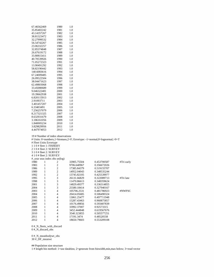
67.46562469 1980 1.0 35.85402242 1981 1.0 43.14357267 1982 1.0 38.81323472 1983 1.0 32.27999532 1984 1.0 56.54742267 1985 1.0 23.06332257 1986 1.0 32.85374848 1987 1.0 26.67619172 1988 1.0 33.80815411 1989 1.0 40.70539926 1990 1.0 71.05272323 1991 1.0 13.90491292 1992 1.0 58.82190442 1993 1.0 140.6083616 1994 1.0 67.24009485 1995 1.0 26.09522504 1996 1.0 38.04471623 1997 1.0 62.49803068 1998 1.0 33.45080689 1999 1.0 9.046322481 2000 1.0 19.39662938 2001 1.0 6.820115913 2002 1.0 2.91093711 2003 1.0 3.401457207 2004 1.0 6.33403491 2005 1.0 7.256257079 2006 1.0 8.217321325 2007 1.0 8.632931679 2008 1.0 3.186161056 2009 1.0 1.840005234 2010 1.0 3.829829956 2011 1.0 4.447974053 2012 1.0 19 # Number of index observations # Units: 0=numbers,1=biomass,2=F; Errortype: -1=normal,0=lognormal,>0=T # Fleet Units Errortype 1 1 0 # fleet 1: FISHERY 2 1 0 # fleet 2: SURVEY 3 1 0 # fleet 2: SURVEY 4 1 0 # fleet 2: SURVEY #_year seas index obs se(log) 1980 1 2 33905.75504 0.453700587 #Tri early 1983 1 2 9706.640967 0.356672026 1986 1 2 17385.84379 0.519155707 1989 1 2 14952.04043 0.348535244 1992 1 2 13745.82105 0.425539977 1995 1 3 26131.66829 0.322089713 #Tri late 1998 1 3 11470.86613 0.348359624 2001 1 3 14829.49377 0.336314855 2004 1 3 25580.18414 0.327940167 2003 1 4 105706.2531 0.481786923 #NWFSC 2004 1 4 20414.05685 0.506490324 2005 1 4 13061.25477 0.497711948 2006 1 4 15287.43463 0.960875857 2007 1 4 10176.49856 0.593407839 2008 1 4 33992.37007 0.92573315 2009 1 4 3452.444848 0.619567676 2010 1 4 3540.323855 0.505577251 2011 1 4 17191.3474 0.48520558 2012 1 4 18650.79603 0.553209108 0 #_N_fleets_with_discard 0 #_N_discard_obs 0 #_N_meanbodywt_obs 30 #_DF_meanwt ## Population size structure 1 # length bin method: 1=use databins; 2=generate from binwidth,min,max below; 3=read vector

256

# binwidth for population size comp # minimum size in the population (lower edge of first bin and size at age 0.00) # maximum size in the population (lower edge of last bin) -1 #_comp_tail_compression 1e-007 #_add_to_comp 0 #_combine males into females at or below this bin number 20 #_N_LengthBins 2 4 6 8 10 12 14 16 18 20 22 24 26 28 30 32 34 36 38 40 0 #_N_Length_obs #Yr Seas Flt/Svy Gender Part Nsamp datavector(female-male) 34 #_N_age_bins 1 2 3 4 5 6 7 8 9 10 11 12 13 14 15 16 17 18 19 20 21 22 23 24 25 26 27 28 29 30 31 32 33 34 0 #_N_ageerror_definitions 0 #_N_Agecomp_obs 1 #_Lbin_method: 1=poplenbins; 2=datalenbins; 3=lengths 0 #_combine males into females at or below this bin number 0 #_N_MeanSize-at-Age_obs 0 #_N_environ_variables 0 #_N_environ_obs 0 # N sizefreq methods to read 0 # no tag data 0 # no morphcomp data 999 # End data file Control file #C growth parameters are estimated 1 #_N_Growth_Patterns 1 #_N_Morphs_Within_GrowthPattern 0 #_Nblock_Patterns #_Cond 0 #_blocks_per_pattern # begin and end years of blocks # 0.5 #_fracfemale 0 #_natM_type:_0=1Parm; 1=N_breakpoints;_2=Lorenzen;_3=agespecific;_4=agespec_withseasinterpolate #_no additional input for selected M option; read 1P per morph 1 # GrowthModel: 1=vonBert with L1andL2; 2=Richards with L1andL2; 3=not implemented; 4=not implemented 1 #_Growth_Age_for_L1 999 #_Growth_Age_for_L2 (999 to use as Linf) 0 #_SD_add_to_LAA (set to 0.1 for SS2 V1.x compatibility) 0 #_CV_Growth_Pattern 1 #_maturity_option: 1=length logistic 4 #_First_Mature_Age 1 #_fecundity option:(1)eggs=Wt*(a+b*Wt);(2)eggs=a*L^b;(3)eggs=a*Wt^b 0 #_hermaphroditism option: 0=none; 1=age-specific fxn 1 #_parameter_offset_approach (1=none, 2= M, G, CV_G as offset from female-GP1, 3=like SS2 V1.x) 2 #_env/block/dev_adjust_method (1=standard; 2=logistic transform keeps in base parm bounds; 3=standard w/ no bound check) # #_growth_parms #_LO HI INIT PRIOR PR_type SD PHASE env-var use_dev dev_minyr dev_maxyr dev_stddev Block Block_Fxn 0.001 2 0.121 -2.112 3 0.4 1 0 0 0 0 0 0 0 # NatM_p_1_Fem_GP_1 1 18.94836209 9.474181043 36 -1 10 -2 0 0 0 0 0 0 0 # L_at_Amin_Fem_GP_1 1 66.1 33.05 70 -1 10 -4 0 0 0 0 0 0 0 # L_at_Amax_Fem_GP_1 0.05 0.12 0.06 0.15 -1 0.8 -4 0 0 0 0 0 0 0 # VonBert_K_Fem_GP_1 0.05 0.2 0.1 0.1 -1 0.8 -3 0 0 0 0 0 0 0 # CV_young_Fem_GP_1 0.05 0.2 0.1 0.1 -1 0.8 -3 0 0 0 0 0 0 0 # CV_old_Fem_GP_1 0.001 2 0.121 -2.112 3 0.4 2 0 0 0 0 0 0 0 # NatM_p_1_Mal_GP_1 1 18.94836209 10.37 36 -1 10 -2 0 0 0 0 0 0 0 # L_at_Amin_Mal_GP_1 1 66.1 17.38 70 -1 10 -4 0 0 0 0 0 0 0 # L_at_Amax_Mal_GP_1 0.05 0.12 0.019 0.15 -1 0.8 -4 0 0 0 0 0 0 0 # VonBert_K_Mal_GP_1 0.05 0.2 0.1 0.1 -1 0.8 -3 0 0 0 0 0 0 0 # CV_young_Mal_GP_1

257

0.05 0.2 0.1 0.1 -1 0.8 -3 0 0 0 0 0 0 0 # CV_old_Mal_GP_1 -3 3 1.68E-05 2.44E-06 -1 0.8 -3 0 0 0 0 0 0 0 # Wtlen_1_Fem -3 4 2.95 3.34694 -1 0.8 -3 0 0 0 0 0 0 0 # Wtlen_2_Fem 1 1000 17 3 -1 0.8 -3 0 0 0 0 0 0 0 # Mat50%_Fem -30 3 -2.30 -0.25 -1 0.8 -3 0 0 0 0 0 0 0 # Mat_slope_Fem -3 3 1 1 -1 0.8 -3 0 0 0 0 0 0 0 # Eggs/kg_inter_Fem -3 3 0 0 -1 0.8 -3 0 0 0 0 0 0 0 # Eggs/kg_slope_wt_Fem -3 3 2.98E-05 2.44E-06 -1 0.8 -3 0 0 0 0 0 0 0 # Wtlen_1_Mal -3 4 2.72 3.34694 -1 0.8 -3 0 0 0 0 0 0 0 # Wtlen_2_Mal 0 0 0 0 -1 0 -4 0 0 0 0 0 0 0 # RecrDist_GP_1 0 0 0 0 -1 0 -4 0 0 0 0 0 0 0 # RecrDist_Area_1 0 0 0 0 -1 0 -4 0 0 0 0 0 0 0 # RecrDist_Seas_1 0 0 0 0 -1 0 -4 0 0 0 0 0 0 0 # CohortGrowDev # #_seasonal_effects_on_biology_parms 0 0 0 0 0 0 0 0 0 0#_Spawner-Recruitment 3 #_SR_function #_LO HI INIT PRIOR PR_type SD PHASE 1 31 10 2.3 -1 3 1 #-1 10 1 # SR_R0 0.25 0.99 0.4 0.779 2 0.152 3 # SR_steep # SR_steep 0 2 0.01 0.8 -1 0.8 -4 # SR_sigmaR -5 5 0.1 0 -1 1 -3 # SR_envlink -5 5 0 0 -1 1 -4 # SR_R1_offset 0 0 0 0 -1 0 -99 # SR_autocorr 0 #_SR_env_link 0 #_SR_env_target_0=none;1=devs;_2=R0;_3=steepness 0 #do_recdev: 0=none; 1=devvector; 2=simple deviations 2012 # first year of main recr_devs 2012 # last year of main recr_devs -2 #_recdev phase 1 # (0/1) to read 13 advanced options 0 #_recdev_early_start (0=none; neg value makes relative to recdev_start) -4 #_recdev_early_phase -1 #_forecast_recruitment 1 #_lambda for fore_recr_like occurring before endyr+1 1990 #_last_early_yr_nobias_adj_in_MPD 1999 #_first_yr_fullbias_adj_in_MPD 2000 #_last_yr_fullbias_adj_in_MPD 2012 #_first_recent_yr_nobias_adj_in_MPD 1.0 #_max_bias_adj_in_MPD 0 #_period of cycles in recruitment (N parms read below) -5 #min rec_dev 5 #max rec_dev 0 #_read_recdevs #Fishing Mortality info 0.3 # F ballpark for tuning early phases -2001 # F ballpark year (neg value to disable) 1 # F_Method: 1=Pope; 2=instan. F; 3=hybrid (hybrid is recommended) 0.9 # max F or harvest rate, depends on F_Method #_initial_F_parms #_LO HI INIT PRIOR PR_type SD PHASE 0 1 0 0.01 0 99 -1 # InitF_1FISHERY1 #_Q_setup # Q_type options: <0=mirror, 0=median_float, 1=mean_float, 2=parameter, 3=parm_w_random_dev, 4=parm_w_randwalk, 5=mean_unbiased_float_assign_to_parm #_Den-dep env-var extra_se Q_type 0 0 0 0 # 1 FISHERY1

258

# ADDS EXTRA SD TO SURVEYS 0 0 1 0 # 2 SURVEY1 0 0 1 0 # 3 SURVEY2 0 0 1 0 # 4 SURVEY3 # #_Cond 0 #_If q has random component, then 0=read one parm for each fleet with random q; 1=read a parm for each year of index #_Q_parms(if_any) # LO HI INIT PRIOR PR_type SD PHASE 0 5 0.01 0.01 0 99 1 # InitF_1FISHERY1 0 5 0.01 0.01 0 99 1 # InitF_1FISHERY1 0 5 0.01 0.01 0 99 1 # InitF_1FISHERY1 #_size_selex_types #_Pattern Discard Male Special 1 0 0 0 # 1 FISHERY1 1 0 0 0 # 2 SURVEY1 1 0 0 0 # 2 SURVEY1 1 0 0 0 # 2 SURVEY1 # #_age_selex_types #_Pattern ___ Male Special 10 0 0 0 # 1 FISHERY1 10 0 0 0 # 2 SURVEY1 10 0 0 0 # 2 SURVEY1 10 0 0 0 # 2 SURVEY1 #_LO HI INIT PRIOR PR_type SD PHASE env-var use_dev dev_minyr dev_maxyr dev_stddev Block Block_Fxn 0 40 17 4 -1 99 -1 0 0 0 0 0 0 0 # AgeSel_1P_1_FISHERY1 0 40 1.280191 38 -1 99 -1 0 0 0 0 0 0 0 # AgeSel_1P_2_FISHERY1 0 40 17 4 -1 99 -1 0 0 0 0 0 0 0 # AgeSel_1P_1_FISHERY1 0 40 1.280191 38 -1 99 -1 0 0 0 0 0 0 0 # AgeSel_1P_2_FISHERY1 0 40 17 4 -1 99 -1 0 0 0 0 0 0 0 # AgeSel_1P_1_FISHERY1 0 40 1.280191 38 -1 99 -1 0 0 0 0 0 0 0 # AgeSel_1P_2_FISHERY1 0 40 17 4 -1 99 -1 0 0 0 0 0 0 0 # AgeSel_1P_1_FISHERY1 0 40 1.280191 38 -1 99 -1 0 0 0 0 0 0 0 # AgeSel_1P_2_FISHERY1 # Tag loss and Tag reporting parameters go next 0 # TG_custom: 0=no read; 1=read if tags exist #_Cond -6 6 1 1 2 0.01 -4 0 0 0 0 0 0 0 #_placeholder if no parameters # 0 #_Variance_adjustments_to_input_values 1 #_maxlambdaphase 1 #_sd_offset # 0 # number of changes to make to default Lambdas (default value is 1.0) 0 # (0/1) read specs for more stddev reporting 999 Starter file #C starter comment here STRK_data.ss STRK_control.ctl 0 # 0=use init values in control file; 1=use ss3.par 0 # run display detail (0,1,2) 0 # detailed age-structured reports in REPORT.SSO (0,1) 1 # write detailed checkup.sso file (0,1) 4 # write parm values to ParmTrace.sso (0=no,1=good,active; 2=good,all; 3=every_iter,all_parms; 4=every,active) 1 # write to cumreport.sso (0=no,1=likeandtimeseries; 2=add survey fits) 1 # Include prior_like for non-estimated parameters (0,1) 1 # Use Soft Boundaries to aid convergence (0,1) (recommended) 1 # Number of bootstrap datafiles to produce 6 # Turn off estimation for parameters entering after this phase 1 # MCeval burn interval 1 # MCeval thin interval 0.1 # jitter initial parm value by this fraction -1 # min yr for sdreport outputs (-1 for styr) -2 # max yr for sdreport outputs (-1 for endyr; -2 for endyr+Nforecastyrs 0 # N individual STD years #vector of year values 0.0001 # final convergence criteria (e.g., 1.0e-04) 0 # retrospective year relative to end year (e.g., -4)

259

0 # min age for calc of summary biomass 1 # Depletion basis: denom is: 0=skip; 1=rel X*B0; 2=rel X*Bmsy; 3=rel X*B_styr 1 # Fraction (X) for Depletion denominator (e.g., 0.4) 1 # SPR_report_basis: 0=skip; 1=(1-SPR)/(1-SPR_tgt); 2=(1-SPR)/(1-SPR_MSY); 3=(1-SPR)/(1-SPR_Btarget); 4=rawSPR 3 # F_report_units: 0=skip; 1=exploitation(Bio); 2=exploitation(Num); 3=sum(Frates) 2 # F_report_basis: 0=raw; 1=F/Fspr; 2=F/Fmsy ; 3=F/Fbtgt 999 # check value for end of file Forecast file 1 # Benchmarks: 0=skip; 1=calc F_spr,F_btgt,F_msy 2 # MSY: 1= set to F(SPR); 2=calc F(MSY); 3=set to F(Btgt); 4=set to F(endyr) 0.5 # SPR target (e.g., 0.40) 0.4 # Biomass target (e.g., 0.40) #_Bmark_years: beg_bio, end_bio, beg_selex, end_selex, beg_relF, end_relF (enter actual year, or values of 0 or -integer to be rel. endyr) 0 0 0 0 0 0 # 2010 2010 2010 2010 2010 2010 # after processing 1 #Bmark_relF_Basis: 1 = use year range; 2 = set relF same as forecast below # 1 # Forecast: 0=none; 1=F(SPR); 2=F(MSY) 3=F(Btgt); 4=Ave F (uses first-last relF yrs); 5=input annual F scalar 12 # N forecast years 0.2 # F scalar (only used for Do_Forecast==5) #_Fcast_years: beg_selex, end_selex, beg_relF, end_relF (enter actual year, or values of 0 or -integer to be rel. endyr) 0 0 0 0 # 2010 2010 2010 2010 # after processing 1 # Control rule method (1=catch=f(SSB) west coast; 2=F=f(SSB) ) 0.4 # Control rule Biomass level for constant F (as frac of Bzero, e.g., 0.40); (Must be > the no F level below) 0.1 # Control rule Biomass level for no F (as frac of Bzero, e.g., 0.10) 1 # Control rule target as fraction of Flimit (e.g., 0.75) 3 #_N forecast loops (1=OFL only; 2=ABC; 3=get F from forecast ABC catch with allocations applied) 3 #_First forecast loop with stochastic recruitment 0 #_Forecast loop control #3 (reserved for future bellsandwhistles) 0 #_Forecast loop control #4 (reserved for future bellsandwhistles) 0 #_Forecast loop control #5 (reserved for future bellsandwhistles) 2013 #FirstYear for caps and allocations (should be after years with fixed inputs) 0 # stddev of log(realized catch/target catch) in forecast (set value>0.0 to cause active impl_error) 0 # Do West Coast gfish rebuilder output (0/1) 2013 # Rebuilder: first year catch could have been set to zero (Ydecl)(-1 to set to 1999) 2013 # Rebuilder: year for current age structure (Yinit) (-1 to set to endyear+1) 1 # fleet relative F: 1=use first-last alloc year; 2=read seas(row) x fleet(col) below # Note that fleet allocation is used directly as average F if Do_Forecast=4 2 # basis for fcast catch tuning and for fcast catch caps and allocation (2=deadbio; 3=retainbio; 5=deadnum; 6=retainnum) # Conditional input if relative F choice = 2 # Fleet relative F: rows are seasons, columns are fleets #_Fleet: FISHERY # 1 # max totalcatch by fleet (-1 to have no max) must enter value for each fleet -1 # max totalcatch by area (-1 to have no max); must enter value for each fleet -1 # fleet assignment to allocation group (enter group ID# for each fleet, 0 for not included in an alloc group) 0 #_Conditional on >1 allocation group # allocation fraction for each of: 0 allocation groups # no allocation groups 2 # Number of forecast catch levels to input (else calc catch from forecast F) 2 # basis for input Fcast catch: 2=dead catch; 3=retained catch; 99=input Hrate(F) (units are from fleetunits; note new codes in SSV3.20) # Input fixed catch values #Year Seas Fleet Catch(or_F) 2013 1 1 3.4 2014 1 1 3.4 999 # verify end of input Appendix A.3. Yellowtail rockfish (North of 40° 10′ N lat.) Data file # Data-mod 2013: YELLOWTAIL NORTH ROCKFISH

260

######################################## ### Global model specifications ### 1892 # Start year 2012 # End year 1 # Number of seasons/year 12 # Number of months/season 1 # Spawning occurs at beginning of season 1 # Number of fishing fleets 2 # Number of surveys 1 # Number of areas FISHERY%Triennial%NWFSC 0.5 0.5 0.5 # fleet timing_in_season 1 1 1 # Area of each fleet 1 # Units for catch by fishing fleet: 1=Biomass(mt),2=Numbers(1000s) 0.01 # SE of log(catch) by fleet for equilibrium and continuous options 2 # Number of genders 64 # Number of ages in population dynamics ### Catch section ### 0 # Initial equilibrium catch (landings + discard) by fishing fleet 121 # Number of lines of catch # Catch Year Season 2.179923641 1892 1.0 2.179923641 1893 1.0 2.179923641 1894 1.0 0.560555063 1895 1.0 0.134944203 1896 1.0 0.137546252 1897 1.0 0.077851691 1898 1.0 0.131677636 1899 1.0 0.185503581 1900 1.0 0.239319989 1901 1.0 0.293145934 1902 1.0 0.346971879 1903 1.0 0.400797824 1904 1.0 0.454614232 1905 1.0 0.508440177 1906 1.0 0.562266122 1907 1.0 0.61608253 1908 1.0 0.669908475 1909 1.0 0.72373442 1910 1.0 0.777560365 1911 1.0 0.831376773 1912 1.0 0.885202718 1913 1.0 0.939028663 1914 1.0 0.992854608 1915 1.0 3.035198871 1916 1.0 5.013428734 1917 1.0 10.2907837 1918 1.0 3.307769605 1919 1.0 4.113251535 1920 1.0 5.592206255 1921 1.0 4.556611093 1922 1.0 2.467933617 1923 1.0 4.333689409 1924 1.0 10.79270794 1925 1.0 10.72067684 1926 1.0 18.97511125 1927 1.0 17.70551093 1928 1.0 26.02660946 1929 1.0 36.91904695 1930 1.0 41.93393506 1931 1.0 27.92354337 1932 1.0 25.96381366 1933 1.0 22.91444839 1934 1.0 34.89300721 1935 1.0 40.0264671 1936 1.0 48.18266148 1937 1.0 55.26373671 1938 1.0

261

62.69846195 1939 1.0 140.3158232 1940 1.0 188.6193066 1941 1.0 341.3979187 1942 1.0 1116.685285 1943 1.0 1936.512538 1944 1.0 3390.804562 1945 1.0 2201.014236 1946 1.0 1208.997327 1947 1.0 1076.03877 1948 1.0 951.8411821 1949 1.0 961.3926344 1950 1.0 855.0280503 1951 1.0 1008.617746 1952 1.0 796.0048183 1953 1.0 1147.37031 1954 1.0 975.5500468 1955 1.0 1475.458455 1956 1.0 1610.51716 1957 1.0 1434.977317 1958 1.0 1588.919666 1959 1.0 1994.718096 1960 1.0 1963.126365 1961 1.0 2447.958202 1962 1.0 1900.84491 1963 1.0 1598.463435 1964 1.0 1573.934988 1965 1.0 4896.570072 1966 1.0 3016.479951 1967 1.0 3321.470042 1968 1.0 3821.105623 1969 1.0 2215.580474 1970 1.0 1674.707728 1971 1.0 2533.196617 1972 1.0 2347.888846 1973 1.0 1702.736483 1974 1.0 1428.225223 1975 1.0 4324.366471 1976 1.0 5086.99836 1977 1.0 8282.488631 1978 1.0 8047.547628 1979 1.0 7889.58503 1980 1.0 9298.114289 1981 1.0 9799.270236 1982 1.0 8931.041533 1983 1.0 5521.196029 1984 1.0 3769.608425 1985 1.0 5397.855277 1986 1.0 5268.109663 1987 1.0 6956.758651 1988 1.0 6181.381485 1989 1.0 5237.915225 1990 1.0 5285.164195 1991 1.0 8376.061302 1992 1.0 7708.453412 1993 1.0 7584.348398 1994 1.0 6857.312783 1995 1.0 8673.571917 1996 1.0 3151.101658 1997 1.0 4214.202876 1998 1.0 4816.414211 1999 1.0 5011.828389 2000 1.0 3387.202805 2001 1.0 2452.138452 2002 1.0 1490.018131 2003 1.0 1750.188782 2004 1.0 966.080702 2005 1.0 510.8182355 2006 1.0 405.3577101 2007 1.0 511.0469504 2008 1.0

262

817.3896664 2009 1.0 1026.606114 2010 1.0 1456.016121 2011 1.0 1646.362201 2012 1.0 19 # Number of index observations # Units: 0=numbers,1=biomass,2=F; Errortype: -1=normal,0=lognormal,>0=T # Fleet Units Errortype 1 1 0 # fleet 1: FISHERY 2 1 0 # fleet 2: SURVEY 3 1 0 # fleet 2: SURVEY #_year seas index obs se(log) 1980 1 2 8962.196869 0.334858607 #Tri 1983 1 2 13130.56899 0.191635919 1986 1 2 9855.239779 0.278644309 1989 1 2 6539.568103 0.286905232 1992 1 2 8630.494905 0.2667461 1995 1 2 2924.167225 0.303715645 1998 1 2 21151.41523 0.305317909 2001 1 2 5021.728611 0.319566943 2004 1 2 17350.23909 0.845518222 2003 1 3 21205.26474 0.473755244 #NWFSC 2004 1 3 19239.33425 0.552662098 2005 1 3 23343.35736 0.43220822 2006 1 3 9036.145701 0.474465699 2007 1 3 16088.99761 0.435602184 2008 1 3 14246.9584 0.470159183 2009 1 3 7320.101698 0.473810099 2010 1 3 37589.2747 0.417056884 2011 1 3 25480.36039 0.424339276 2012 1 3 14678.0086 0.440904381 0 #_N_fleets_with_discard 0 #_N_discard_obs 0 #_N_meanbodywt_obs 30 #_DF_meanwt ## Population size structure 1 # length bin method: 1=use databins; 2=generate from binwidth,min,max below; 3=read vector -1 #_comp_tail_compression 1e-007 #_add_to_comp 0 #_combine males into females at or below this bin number 33 #_N_LengthBins 2 4 6 8 10 12 14 16 18 20 22 24 26 28 30 32 34 36 38 40 42 44 46 48 50 52 54 56 58 60 62 64 66 0 #_N_Length_obs #Yr Seas Flt/Svy Gender Part Nsamp datavector(female-male) 58 #_N_age_bins 1 2 3 4 5 6 7 8 9 10 11 12 13 14 15 16 17 18 19 20 21 22 23 24 25 26 27 28 29 30 31 32 33 34 35 36 37 38 39 40 41 42 43 44 45 46 47 48 49 50 51 52 53 54 55 56 57 58 0 #_N_ageerror_definitions 0 #_N_Agecomp_obs 1 #_Lbin_method: 1=poplenbins; 2=datalenbins; 3=lengths 0 #_combine males into females at or below this bin number 0 #_N_MeanSize-at-Age_obs 0 #_N_environ_variables 0 #_N_environ_obs 0 # N sizefreq methods to read 0 # no tag data 0 # no morphcomp data 999 # End data file Control file

263

#C growth parameters are estimated 1 #_N_Growth_Patterns 1 #_N_Morphs_Within_GrowthPattern 0 #_Nblock_Patterns 0.5 #_fracfemale 0 #_natM_type:_0=1Parm; 1=N_breakpoints;_2=Lorenzen;_3=agespecific;_4=agespec_withseasinterpolate #_no additional input for selected M option; read 1P per morph 1 # GrowthModel: 1=vonBert with L1andL2; 2=Richards with L1andL2; 3=not implemented; 4=not implemented 1 #_Growth_Age_for_L1 999 #_Growth_Age_for_L2 (999 to use as Linf) 0 #_SD_add_to_LAA (set to 0.1 for SS2 V1.x compatibility) 0 #_CV_Growth_Pattern: 0 CV=f(LAA); 1 CV=F(A); 2 SD=F(LAA); 3 SD=F(A) 1 #_maturity_option: 1=length logistic; 2=age logistic; 3=read age-maturity matrix by growth_pattern; 4=read age-fecundity; 5=read fec and wt from wtatage.ss #_placeholder for empirical age-maturity by growth pattern 0 #_First_Mature_Age 1 #_fecundity option:(1)eggs=Wt*(a+b*Wt);(2)eggs=a*L^b;(3)eggs=a*Wt^b 0 #_hermaphroditism option: 0=none; 1=age-specific fxn 1 #_parameter_offset_approach (1=none, 2= M, G, CV_G as offset from female-GP1, 3=like SS2 V1.x) 2 #_env/block/dev_adjust_method (1=standard; 2=logistic transform keeps in base parm bounds; 3=standard w/ no bound check) # #_growth_parms #_LO HI INIT PRIOR PR_type SD PHASE env-var use_dev dev_minyr dev_maxyr dev_stddev Block Block_Fxn 0.001 2 0.11 -2.207 3 0.4 2 0 0 0 0 0 0 0 # NatM_p_1_Fem_GP_1 1 26.87012886 13.43506443 36 -1 10 -2 0 0 0 0 0 0 0 # L_at_Amin_Fem_GP_1 1 104.42 52.21 70 -1 10 -4 0 0 0 0 0 0 0 # L_at_Amax_Fem_GP_1 0.05 0.34 0.17 0.15 -1 0.8 -4 0 0 0 0 0 0 0 # VonBert_K_Fem_GP_1 0.05 0.2 0.1 0.1 -1 0.8 -3 0 0 0 0 0 0 0 # CV_young_Fem_GP_1 0.05 0.2 0.1 0.1 -1 0.8 -3 0 0 0 0 0 0 0 # CV_old_Fem_GP_1 0.001 2 0.11 -2.207 3 0.4 2 0 0 0 0 0 0 0 # NatM_p_1_Mal_GP_1 1 26.87012886 12.51 36 -1 10 -2 0 0 0 0 0 0 0 # L_at_Amin_Mal_GP_1 1 104.42 47.57 70 -1 10 -4 0 0 0 0 0 0 0 # L_at_Amax_Mal_GP_1 0.05 0.34 0.19 0.15 -1 0.8 -4 0 0 0 0 0 0 0 # VonBert_K_Mal_GP_1 0.05 0.2 0.1 0.1 -1 0.8 -3 0 0 0 0 0 0 0 # CV_young_Mal_GP_1 0.05 0.2 0.1 0.1 -1 0.8 -3 0 0 0 0 0 0 0 # CV_old_Mal_GP_1 -3 3 1.32E-05 2.44E-06 -1 0.8 -3 0 0 0 0 0 0 0 # Wtlen_1_Fem -3 4 3.03 3.34694 -1 0.8 -3 0 0 0 0 0 0 0 # Wtlen_2_Fem 1 1000 37 9 -1 0.8 -3 0 0 0 0 0 0 0 # Mat50%_Fem -30 3 -0.47 -0.25 -1 0.8 -3 0 0 0 0 0 0 0 # Mat_slope_Fem -3 3 1 1 -1 0.8 -3 0 0 0 0 0 0 0 # Eggs/kg_inter_Fem -3 3 0 0 -1 0.8 -3 0 0 0 0 0 0 0 # Eggs/kg_slope_wt_Fem -3 3 1.24E-05 2.44E-06 -1 0.8 -3 0 0 0 0 0 0 0 # Wtlen_1_Mal -3 4 3.06 3.34694 -1 0.8 -3 0 0 0 0 0 0 0 # Wtlen_2_Mal 0 0 0 0 -1 0 -4 0 0 0 0 0 0 0 # RecrDist_GP_1 0 0 0 0 -1 0 -4 0 0 0 0 0 0 0 # RecrDist_Area_1 0 0 0 0 -1 0 -4 0 0 0 0 0 0 0 # RecrDist_Seas_1 0 0 0 0 -1 0 -4 0 0 0 0 0 0 0 # CohortGrowDev # #_seasonal_effects_on_biology_parms 0 0 0 0 0 0 0 0 0 0 #_Spawner-Recruitment 3 #_SR_function

264

#_LO HI INIT PRIOR PR_type SD PHASE 1 31 12.2 12.2 -1 10 1 # SR_R0 0.25 0.99 0.779 0.779 2 0.152 3 # SR_steep 0 2 0.01 0.8 -1 0.8 -4 # SR_sigmaR -5 5 0.1 0 -1 1 -3 # SR_envlink -5 5 0 0 -1 1 -4 # SR_R1_offset 0 0 0 0 -1 0 -99 # SR_autocorr 0 #_SR_env_link 0 #_SR_env_target_0=none;1=devs;_2=R0;_3=steepness 0 #do_recdev: 0=none; 1=devvector; 2=simple deviations 2012 # first year of main recr_devs 2012 # last year of main recr_devs -2 #_recdev phase 1 # (0/1) to read 13 advanced options 0 #_recdev_early_start (0=none; neg value makes relative to recdev_start) -4 #_recdev_early_phase -1 #_forecast_recruitment 1 #_lambda for fore_recr_like occurring before endyr+1 1990 #_last_early_yr_nobias_adj_in_MPD 1999 #_first_yr_fullbias_adj_in_MPD 2000 #_last_yr_fullbias_adj_in_MPD 2012 #_first_recent_yr_nobias_adj_in_MPD 1.0 #_max_bias_adj_in_MPD 0 #_period of cycles in recruitment (N parms read below) -5 #min rec_dev 5 #max rec_dev 0 #_read_recdevs #Fishing Mortality info 0.3 # F ballpark for tuning early phases -2001 # F ballpark year (neg value to disable) 1 # F_Method: 1=Pope; 2=instan. F; 3=hybrid (hybrid is recommended) 0.9 # max F or harvest rate, depends on F_Method #_initial_F_parms #_LO HI INIT PRIOR PR_type SD PHASE 0 1 0 0.01 0 99 -1 # InitF_1FISHERY1 #_Q_setup # Q_type options: <0=mirror, 0=median_float, 1=mean_float, 2=parameter, 3=parm_w_random_dev, 4=parm_w_randwalk, 5=mean_unbiased_float_assign_to_parm #_Den-dep env-var extra_se Q_type 0 0 0 0 # 1 FISHERY1 0 0 1 0 # 2 SURVEY1 0 0 1 0 # 2 SURVEY1 #_Cond 0 #_If q has random component, then 0=read one parm for each fleet with random q; 1=read a parm for each year of index #_Q_parms(if_any) # LO HI INIT PRIOR PR_type SD PHASE 0 5 0 0.1 -1 0.1 1 0 5 0 0.1 -1 0.1 1 #_size_selex_types #_Pattern Discard Male Special 1 0 0 0 # 1 FISHERY1 1 0 0 0 # 2 SURVEY1 1 0 0 0 # 2 SURVEY1 #_age_selex_types #_Pattern ___ Male Special 10 0 0 0 # 2 SURVEY1 10 0 0 0 # 2 SURVEY1 10 0 0 0 # 2 SURVEY1 #_LO HI INIT PRIOR PR_type SD PHASE env-var use_dev dev_minyr dev_maxyr dev_stddev Block Block_Fxn 0 40 37 10 -1 99 -1 0 0 0 0 0 0 0 # AgeSel_1P_1_FISHERY1 0 65 6.264764 64 -1 99 -1 0 0 0 0 0 0 0 # AgeSel_1P_2_FISHERY1 0 40 37 10 -1 99 -1 0 0 0 0 0 0 0 # AgeSel_1P_1_FISHERY1 0 65 6.264764 64 -1 99 -1 0 0 0 0 0 0 0 # AgeSel_1P_2_FISHERY1 0 40 37 10 -1 99 -1 0 0 0 0 0 0 0 # AgeSel_1P_1_FISHERY1 0 65 6.264764 64 -1 99 -1 0 0 0 0 0 0 0 # AgeSel_1P_2_FISHERY1 0 # Tagging flag: 0=none,1=read parameters for tagging ### Likelihood related quantities ### # variance/sample size adjustment by fleet 0 # Do variance adjustments 1 # Max N lambda phases: read this N values for each item below 1 # SD offset (CPUE, discard, mean body weight, recruitment devs): 0=omit log(s) term, 1=include

265

0 # N changes to default Lambdas = 1.0 0 # extra SD pointer 999 # end of control file Starter file #C starter comment here YTRK_N_data.ss YTRK_N_control.ss 0 # 0=use init values in control file; 1=use ss3.par 0 # run display detail (0,1,2) 0 # detailed age-structured reports in REPORT.SSO (0,1) 1 # write detailed checkup.sso file (0,1) 4 # write parm values to ParmTrace.sso (0=no,1=good,active; 2=good,all; 3=every_iter,all_parms; 4=every,active) 1 # write to cumreport.sso (0=no,1=likeandtimeseries; 2=add survey fits) 1 # Include prior_like for non-estimated parameters (0,1) 1 # Use Soft Boundaries to aid convergence (0,1) (recommended) 1 # Number of bootstrap datafiles to produce 6 # Turn off estimation for parameters entering after this phase 1 # MCeval burn interval 1 # MCeval thin interval 0.1 # jitter initial parm value by this fraction -1 # min yr for sdreport outputs (-1 for styr) -2 # max yr for sdreport outputs (-1 for endyr; -2 for endyr+Nforecastyrs 0 # N individual STD years #vector of year values 0.0001 # final convergence criteria (e.g., 1.0e-04) 0 # retrospective year relative to end year (e.g., -4) 0 # min age for calc of summary biomass 1 # Depletion basis: denom is: 0=skip; 1=rel X*B0; 2=rel X*Bmsy; 3=rel X*B_styr 1 # Fraction (X) for Depletion denominator (e.g., 0.4) 1 # SPR_report_basis: 0=skip; 1=(1-SPR)/(1-SPR_tgt); 2=(1-SPR)/(1-SPR_MSY); 3=(1-SPR)/(1-SPR_Btarget); 4=rawSPR 3 # F_report_units: 0=skip; 1=exploitation(Bio); 2=exploitation(Num); 3=sum(Frates) 0 # F_report_basis: 0=raw; 1=F/Fspr; 2=F/Fmsy ; 3=F/Fbtgt 999 # check value for end of file Forecast file 1 # Benchmarks: 0=skip; 1=calc F_spr,F_btgt,F_msy 2 # MSY: 1= set to F(SPR); 2=calc F(MSY); 3=set to F(Btgt); 4=set to F(endyr) 0.5 # SPR target (e.g., 0.40) 0.4 # Biomass target (e.g., 0.40) #_Bmark_years: beg_bio, end_bio, beg_selex, end_selex, beg_relF, end_relF (enter actual year, or values of 0 or -integer to be rel. endyr) 0 0 0 0 0 0 # 2010 2010 2010 2010 2010 2010 # after processing 1 #Bmark_relF_Basis: 1 = use year range; 2 = set relF same as forecast below # 1 # Forecast: 0=none; 1=F(SPR); 2=F(MSY) 3=F(Btgt); 4=Ave F (uses first-last relF yrs); 5=input annual F scalar 12 # N forecast years 0.2 # F scalar (only used for Do_Forecast==5) #_Fcast_years: beg_selex, end_selex, beg_relF, end_relF (enter actual year, or values of 0 or -integer to be rel. endyr) 0 0 0 0 # 2010 2010 2010 2010 # after processing 1 # Control rule method (1=catch=f(SSB) west coast; 2=F=f(SSB) ) 0.4 # Control rule Biomass level for constant F (as frac of Bzero, e.g., 0.40); (Must be > the no F level below) 0.1 # Control rule Biomass level for no F (as frac of Bzero, e.g., 0.10) 1 # Control rule target as fraction of Flimit (e.g., 0.75) 3 #_N forecast loops (1=OFL only; 2=ABC; 3=get F from forecast ABC catch with allocations applied) 3 #_First forecast loop with stochastic recruitment 0 #_Forecast loop control #3 (reserved for future bellsandwhistles) 0 #_Forecast loop control #4 (reserved for future bellsandwhistles) 0 #_Forecast loop control #5 (reserved for future bellsandwhistles) 2013 #FirstYear for caps and allocations (should be after years with fixed inputs) 0 # stddev of log(realized catch/target catch) in forecast (set value>0.0 to cause active impl_error) 0 # Do West Coast gfish rebuilder output (0/1) 2013 # Rebuilder: first year catch could have been set to zero (Ydecl)(-1 to set to 1999) 2013 # Rebuilder: year for current age structure (Yinit) (-1 to set to endyear+1) 1 # fleet relative F: 1=use first-last alloc year; 2=read seas(row) x fleet(col) below # Note that fleet allocation is used directly as average F if Do_Forecast=4

266

2 # basis for fcast catch tuning and for fcast catch caps and allocation (2=deadbio; 3=retainbio; 5=deadnum; 6=retainnum) # Conditional input if relative F choice = 2 # Fleet relative F: rows are seasons, columns are fleets #_Fleet: FISHERY # 1 # max totalcatch by fleet (-1 to have no max) must enter value for each fleet -1 # max totalcatch by area (-1 to have no max); must enter value for each fleet -1 # fleet assignment to allocation group (enter group ID# for each fleet, 0 for not included in an alloc group) 0 #_Conditional on >1 allocation group # allocation fraction for each of: 0 allocation groups # no allocation groups 2 # Number of forecast catch levels to input (else calc catch from forecast F) 2 # basis for input Fcast catch: 2=dead catch; 3=retained catch; 99=input Hrate(F) (units are from fleetunits; note new codes in SSV3.20) # Input fixed catch values #Year Seas Fleet Catch(or_F) 2013 1 1 1376.3 2014 1 1 1376.3 999 # verify end of input Appendix A.4. English sole Data file # Data-mod 2013: ENGLISH SOLE ######################################## ### Global model specifications ### 1876 # Start year 2012 # End year 1 # Number of seasons/year 12 # Number of months/season 1 # Spawning occurs at beginning of season 1 # Number of fishing fleets 3 # Number of surveys 1 # Number of areas FISHERY%SURVEY1%SURVEY2%SURVEY3 0.5417 0.5417 0.5417 0.5417 #fleet timing_in_season 1 1 1 1 # Area of each fleet 1 # Units for catch by fishing fleet: 1=Biomass(mt),2=Numbers(1000s) 0.01 # SE of log(catch) by fleet for equilibrium and continuous options 2 # Number of genders 30 # Number of ages in population dynamics ### Catch section ### 0 # Initial equilibrium catch (landings + discard) by fishing fleet 137 # Number of lines of catch # Catch Year Season 1 1876 1 1 1877 1 1 1878 1 2 1879 1 2 1880 1 2 1881 1 3 1882 1 5 1883 1 5 1884 1 6 1885 1 7 1886 1 8 1887 1 10 1888 1 13 1889 1 15 1890 1 17 1891 1 21 1892 1 25 1893 1 31 1894 1 37 1895 1 43 1896 1

267

53 1897 1 63 1898 1 75 1899 1 90 1900 1 109 1901 1 130 1902 1 157 1903 1 189 1904 1 226 1905 1 271 1906 1 326 1907 1 391 1908 1 469 1909 1 564 1910 1 677 1911 1 813 1912 1 977 1913 1 1173 1914 1 1409 1915 1 2826 1916 1 3865 1917 1 3132 1918 1 2475 1919 1 1715 1920 1 2184 1921 1 3159 1922 1 3186 1923 1 4110 1924 1 4018 1925 1 3865 1926 1 4690 1927 1 4143 1928 1 4811 1929 1 3732 1930 1 1928 1931 1 3540 1932 1 3346 1933 1 2845 1934 1 3226 1935 1 3404 1936 1 3159 1937 1 2543 1938 1 2991 1939 1 3038 1940 1 2202 1941 1 2064 1942 1 3638 1943 1 2141 1944 1 1887 1945 1 4998 1946 1 3334 1947 1 6030 1948 1 3546 1949 1 5673 1950 1 4189 1951 1 3824 1952 1 2911 1953 1 2623 1954 1 2829 1955 1 3787 1956 1 4436 1957 1 5520 1958 1 5427 1959 1 4338 1960 1 4188 1961 1 4496 1962 1 4489 1963 1 4742 1964 1 5043 1965 1 5522 1966 1

268

5192 1967 1 5468 1968 1 3788 1969 1 3102 1970 1 2851 1971 1 3300 1972 1 3773 1973 1 3858 1974 1 4579 1975 1 5755 1976 1 3735 1977 1 4511 1978 1 4710 1979 1 4143 1980 1 3780 1981 1 3833 1982 1 3091 1983 1 2458 1984 1 2955 1985 1 3153 1986 1 3979 1987 1 3422 1988 1 3780 1989 1 2907 1990 1 3339 1991 1 2556 1992 1 2534 1993 1 1818 1994 1 1762 1995 1 1540 1996 1 1911 1997 1 1441 1998 1 1245 1999 1 1061 2000 1 1363 2001 1 1683 2002 1 1125 2003 1 1218 2004 1 1115 2005 1 1078 2006 1 789.4 2007 1 420.1 2008 1 415.5 2009 1 258.1 2010 1 198.1 2011 1 216.1 2012 1 19 # Number of index observations # Units: 0=numbers,1=biomass,2=F; Errortype: -1=normal,0=lognormal,>0=T # Fleet Units Errortype 1 1 0 # fleet 1: FISHERY 2 1 0 # fleet 2: SURVEY 3 1 0 # fleet 2: SURVEY 4 1 0 # fleet 2: SURVEY #_year seas index obs se(log) 1980 1 2 5068.04 0.191990701 #Tri early 1983 1 2 11352.60 0.5#0.157586493 1986 1 2 14077.63 0.136826903 1989 1 2 13993.23 0.118986159 1992 1 2 12412.52 0.144787134 1995 1 3 15671.87 0.139753547 #Tri late 1998 1 3 20768.12 0.118109976 2001 1 3 26072.37 0.123467305 2004 1 3 44845.17 0.128683219 2003 1 4 47397.74071 0.14066723 #NWFSC 2004 1 4 54628.85833 0.141405536 2005 1 4 40089.20896 0.125322389 2006 1 4 23917.21089 0.138389159 2007 1 4 20615.2281 0.126679898 2008 1 4 18167.64655 0.133558888

269

2009 1 4 21878.99142 0.139215613 2010 1 4 20955.23688 0.129787034 2011 1 4 24911.2161 0.129060731 2012 1 4 26682.23605 0.135269391 0 #_N_fleets_with_discard 0 #_N_discard_obs 0 #_N_meanbodywt_obs 30 #_DF_meanwt ## Population size structure 1 # length bin method: 1=use databins; 2=generate from binwidth,min,max below; 3=read vector -1 #_comp_tail_compression 1e-007 #_add_to_comp 0 #_combine males into females at or below this bin number 23 #_N_LengthBins 2 4 6 8 10 12 14 16 18 20 22 24 26 28 30 32 34 36 38 40 42 44 46 0 #_N_Length_obs 27 #_N_age_bins 1 2 3 4 5 6 7 8 9 10 11 12 13 14 15 16 17 18 19 20 21 22 23 24 25 26 27 0 #_N_ageerror_definitions 0 #_N_Agecomp_obs 1 #_Lbin_method: 1=poplenbins; 2=datalenbins; 3=lengths 0 #_combine males into females at or below this bin number 0 #_N_MeanSize-at-Age_obs 0 #_N_environ_variables 0 #_N_environ_obs 0 # N sizefreq methods to read 0 # no tag data 0 # no morphcomp data 999 # End data file Control file #C growth parameters are estimated #_data_and_control_files: simple.dat // simple.ctl #_SS-V3.10b-safe;_02/24/2010;_Stock_Synthesis_by_Richard_Methot_(NOAA)_using_ADMB 1 #_N_Growth_Patterns 1 #_N_Morphs_Within_GrowthPattern 0 #_Nblock_Patterns #_Cond 0 #_blocks_per_pattern # begin and end years of blocks # 0.5 #_fracfemale 0 #_natM_type:_0=1Parm; 1=N_breakpoints;_2=Lorenzen;_3=agespecific;_4=agespec_withseasinterpolate #_no additional input for selected M option; read 1P per morph 1 # GrowthModel: 1=vonBert with L1andL2; 2=Richards with L1andL2; 3=not implemented; 4=not implemented 2 #_Growth_Age_for_L1 20 #_Growth_Age_for_L2 (999 to use as Linf) 0 #_SD_add_to_LAA (set to 0.1 for SS2 V1.x compatibility) 0 #_CV_Growth_Pattern 1 #_maturity_option: 1=length logistic 0 #_First_Mature_Age 1 #_fecundity option:(1)eggs=Wt*(a+b*Wt);(2)eggs=a*L^b;(3)eggs=a*Wt^b 0 #_hermaphroditism option: 0=none; 1=age-specific fxn 1 #_parameter_offset_approach (1=none, 2= M, G, CV_G as offset from female-GP1, 3=like SS2 V1.x) 2 #_env/block/dev_adjust_method #_growth_parms #_LO HI INIT PRIOR PR_type SD PHASE env-var use_dev dev_minyr dev_maxyr dev_stddev Block Block_Fxn 0.001 2 0.26 -1.347 3 0.4 2 0 0 0 0 0 0 0 # NatM_p_1_Fem_GP_1 5 25 17.3386 16.37 0 50 -2 0 0 0 0 0 0 0 # L_at_Amin_Fem_GP_1 25 55 40.5617 39.814 0 50 -2 0 0 0 0 0 0 0 # L_at_Amax_Fem_GP_1 0.01 1.5 0.357007 0.39273 0 50 -2 0 0 0 0 0 0 0 # VonBert_K_Fem_GP_1 0.01 0.9 0.102856 0.10145 0 50 -2 0 0 0 0 0 0 0 # CV_young_Fem_GP_1

270

0.01 0.9 0.102856 0.10145 0 50 -2 0 0 0 0 0 0 0 # CV_young_Fem_GP_1 0.001 2 0.26 -1.347 3 0.4 2 0 0 0 0 0 0 0 # NatM_p_1_Fem_GP_1 5 25 17.3386 16.37 0 50 -2 0 0 0 0 0 0 0 # L_at_Amin_Fem_GP_1 25 55 23.9845115903962 39.814 0 50 -2 0 0 0 0 0 0 0 # L_at_Amax_Fem_GP_1 0.01 1.5 0.480107669127594 0.39273 0 50 -2 0 0 0 0 0 0 0 # VonBert_K_Fem_GP_1 0.01 0.9 0.178 0.10145 0 50 -2 0 0 0 0 0 0 0 # CV_young_Fem_GP_1 0.01 0.9 0.178 0.10145 0 50 -2 0 0 0 0 0 0 0 # CV_young_Fem_GP_1 -3 3 0.00000821 0.00000547424 -1 0.8 -3 0 0 0 0 0 0 0 # Wtlen_1_Fem -3 4 3.0226 3.03 -1 0.8 -3 0 0 0 0 0 0 0 # Wtlen_2_Fem 0 50 31 25 -1 0.8 -3 0 0 0 0 0 0 0 # Mat50%_Fem -1 1 -0.6104999 -0.5 -1 0.8 -3 0 0 0 0 0 0 0 # Mat_slope_Fem -3 3 1 1 -1 0.8 -3 0 0 0 0 0 0 0 # Eggs/kg_inter_Fem -3 3 0 0 -1 0.8 -3 0 0 0 0 0 0 0 # Eggs/kg_slope_wt_Fem -3 3 0.00000267 1.55E-05 -1 0.8 -3 0 0 0 0 0 0 0 # Wtlen_1_Mal -3 4 3.25 3.03 -1 0.8 -3 0 0 0 0 0 0 0 # Wtlen_2_Mal 0 0 0 0 -1 0 -4 0 0 0 0 0 0 0 # RecrDist_GP_1 0 0 0 0 -1 0 -4 0 0 0 0 0 0 0 # RecrDist_Area_1 0 0 0 0 -1 0 -4 0 0 0 0 0 0 0 # RecrDist_Seas_1 0 0 0 0 -1 0 -4 0 0 0 0 0 0 0 # CohortGrowDev #_seasonal_effects_on_biology_parms 0 0 0 0 0 0 0 0 0 0 #_Spawner-Recruitment 3 #_SR_function #_LO HI INIT PRIOR PR_type SD PHASE 1 31 10 10 -1 10 1 # SR_R0 0.25 0.99 0.85 0.8 0 0.093 3 # SR_steep 0 2 0.01 0.8 -1 0.8 -4 # SR_sigmaR -5 5 0.1 0 -1 1 -3 # SR_envlink -5 5 0 0 -1 1 -4 # SR_R1_offset 0 0 0 0 -1 0 -99 # SR_autocorr 0 #_SR_env_link 0 #_SR_env_target_0=none;1=devs;_2=R0;_3=steepness 0 #do_recdev: 0=none; 1=devvector; 2=simple deviations 2010 # first year of main recr_devs 2010 # last year of main recr_devs -2 #_recdev phase 1 # (0/1) to read 13 advanced options 0 #_recdev_early_start (0=none; neg value makes relative to recdev_start) -4 #_recdev_early_phase -1 #_forecast_recruitment 1 #_lambda for fore_recr_like occurring before endyr+1 1990 #_last_early_yr_nobias_adj_in_MPD 1999 #_first_yr_fullbias_adj_in_MPD 2000 #_last_yr_fullbias_adj_in_MPD 2010 #_first_recent_yr_nobias_adj_in_MPD 1.0 #_max_bias_adj_in_MPD 0 #_period of cycles in recruitment (N parms read below) -5 #min rec_dev 5 #max rec_dev 0 #_read_recdevs # #Fishing Mortality info

271

0.3 # F ballpark for tuning early phases -2001 # F ballpark year (neg value to disable) 1 # F_Method: 1=Pope; 2=instan. F; 3=hybrid (hybrid is recommended) 0.9 # max F or harvest rate, depends on F_Method #_initial_F_parms #_LO HI INIT PRIOR PR_type SD PHASE 0 1 0 0.01 0 99 -1 # InitF_1FISHERY1 #_Q_setup # A=do power, B=env-var, C=extra SD, D=devtype(<0=mirror, 0/1=none, 2=cons, 3=rand, 4=randwalk); E:0=num/1=bio/2=F, F:-1=norm/0=lognorm/>0=T #_A B C D E F 0 0 0 0 # 1 FISHERY1 0 0 1 0 # 2 SURVEY1 0 0 1 0 # 2 SURVEY1 0 0 1 0 # 2 SURVEY1 # #_Cond 0 #_If q has random component, then 0=read one parm for each fleet with random q; 1=read a parm for each year of index #_Q_parms(if_any) # LO HI INIT PRIOR PR_type SD PHASE 0 1000 0.01 0.01 0 99 1 # InitF_1FISHERY1 0 1000 0.01 0.01 0 99 1 # InitF_1FISHERY1 0 1000 0.01 0.01 0 99 1 # InitF_1FISHERY1 #_size_selex_types #_Pattern Discard Male Special 1 0 0 0 # 1 FISHERY1 1 0 0 0 # 2 SURVEY1 1 0 0 0 # 2 SURVEY1 1 0 0 0 # 2 SURVEY1 # #_age_selex_types #_Pattern ___ Male Special 10 0 0 0 # 1 FISHERY1 10 0 0 0 # 2 SURVEY1 10 0 0 0 # 2 SURVEY1 10 0 0 0 # 2 SURVEY1 #_LO HI INIT PRIOR PR_type SD PHASE env-var use_dev dev_minyr dev_maxyr dev_stddev Block Block_Fxn 0 40 31 83 -1 99 -1 0 0 0 0 0 0 0 # AgeSel_1P_1_FISHERY1 0 80 4.822997 30 -1 99 -1 0 0 0 0 0 0 0 # AgeSel_1P_2_FISHERY1 0 40 31 83 -1 99 -1 0 0 0 0 0 0 0 # AgeSel_1P_1_FISHERY1 0 80 4.822997 30 -1 99 -1 0 0 0 0 0 0 0 # AgeSel_1P_2_FISHERY1 0 40 31 83 -1 99 -1 0 0 0 0 0 0 0 # AgeSel_1P_1_FISHERY1 0 80 4.822997 30 -1 99 -1 0 0 0 0 0 0 0 # AgeSel_1P_2_FISHERY1 0 40 31 83 -1 99 -1 0 0 0 0 0 0 0 # AgeSel_1P_1_FISHERY1 0 80 4.822997 30 -1 99 -1 0 0 0 0 0 0 0 # AgeSel_1P_2_FISHERY1 # Tag loss and Tag reporting parameters go next 0 # TG_custom: 0=no read; 1=read if tags exist #_Cond -6 6 1 1 2 0.01 -4 0 0 0 0 0 0 0 #_placeholder if no parameters # 0 #_Variance_adjustments_to_input_values 1 #_maxlambdaphase 1 #_sd_offset 0 # number of changes to make to default Lambdas (default value is 1.0) 0 # (0/1) read specs for more stddev reporting 999 Starter file ENGL_data.ss #_datfile ENGL_control.ss #_datfile #control_modified.ss #_ctlfile 0 #_init_values_src 0 #_run_display_detail 0 #_detailed_age_structure 1 #_checkup 4 #_parmtrace 1 #_cumreport 1 #_prior_like 1 #_soft_bounds 1 #_N_bootstraps 6 #_last_estimation_phase

272

1 #_MCMCburn 1 #_MCMCthin 0.5 #_jitter_fraction -1 #_minyr_sdreport -2 #_maxyr_sdreport 0 #_N_STD_yrs 1e-04 #_converge_criterion 0 #_retro_yr 0 #_min_age_summary_bio 1 #_depl_basis 1 #_depl_denom_frac 1 #_SPR_basis 3 #_F_report_units 0 #_F_report_basis # 999 Forecast file 1 # Benchmarks: 0=skip; 1=calc F_spr,F_btgt,F_msy 2 # MSY: 1= set to F(SPR); 2=calc F(MSY); 3=set to F(Btgt); 4=set to F(endyr) 0.3 # SPR target (e.g., 0.40) 0.25 # Biomass target (e.g., 0.40) #_Bmark_years: beg_bio, end_bio, beg_selex, end_selex, beg_relF, end_relF (enter actual year, or values of 0 or -integer to be rel. endyr) 0 0 0 0 0 0 # 2010 2010 2010 2010 2010 2010 # after processing 1 #Bmark_relF_Basis: 1 = use year range; 2 = set relF same as forecast below # 1 # Forecast: 0=none; 1=F(SPR); 2=F(MSY) 3=F(Btgt); 4=Ave F (uses first-last relF yrs); 5=input annual F scalar 12 # N forecast years 0.2 # F scalar (only used for Do_Forecast==5) #_Fcast_years: beg_selex, end_selex, beg_relF, end_relF (enter actual year, or values of 0 or -integer to be rel. endyr) 0 0 0 0 # 2010 2010 2010 2010 # after processing 1 # Control rule method (1=catch=f(SSB) west coast; 2=F=f(SSB) ) 0.25 # Control rule Biomass level for constant F (as frac of Bzero, e.g., 0.40); (Must be > the no F level below) 0.05 # Control rule Biomass level for no F (as frac of Bzero, e.g., 0.10) 1 # Control rule target as fraction of Flimit (e.g., 0.75) 3 #_N forecast loops (1=OFL only; 2=ABC; 3=get F from forecast ABC catch with allocations applied) 3 #_First forecast loop with stochastic recruitment 0 #_Forecast loop control #3 (reserved for future bellsandwhistles) 0 #_Forecast loop control #4 (reserved for future bellsandwhistles) 0 #_Forecast loop control #5 (reserved for future bellsandwhistles) 2013 #FirstYear for caps and allocations (should be after years with fixed inputs) 0 # stddev of log(realized catch/target catch) in forecast (set value>0.0 to cause active impl_error) 0 # Do West Coast gfish rebuilder output (0/1) 2013 # Rebuilder: first year catch could have been set to zero (Ydecl)(-1 to set to 1999) 2013 # Rebuilder: year for current age structure (Yinit) (-1 to set to endyear+1) 1 # fleet relative F: 1=use first-last alloc year; 2=read seas(row) x fleet(col) below # Note that fleet allocation is used directly as average F if Do_Forecast=4 2 # basis for fcast catch tuning and for fcast catch caps and allocation (2=deadbio; 3=retainbio; 5=deadnum; 6=retainnum) # Conditional input if relative F choice = 2 # Fleet relative F: rows are seasons, columns are fleets #_Fleet: FISHERY # 1 # max totalcatch by fleet (-1 to have no max) must enter value for each fleet -1 # max totalcatch by area (-1 to have no max); must enter value for each fleet -1 # fleet assignment to allocation group (enter group ID# for each fleet, 0 for not included in an alloc group) 0 #_Conditional on >1 allocation group # allocation fraction for each of: 0 allocation groups # no allocation groups 2 # Number of forecast catch levels to input (else calc catch from forecast F) 3 # basis for input Fcast catch: 2=dead catch; 3=retained catch; 99=input Hrate(F) (units are from fleetunits; note new codes in SSV3.20) # Input fixed catch values #Year Seas Fleet Catch(or_F)

273

2013 1 1 224.1 2014 1 1 224.1 999 # verify end of input Appendix A.5. Rex sole Data file # Data-mod 2013: REX SOLE ######################################## ### Global model specifications ### 1896 # Start year 2012 # End year 1 # Number of seasons/year 12 # Number of months/season 1 # Spawning occurs at beginning of season 1 # Number of fishing fleets 3 # Number of surveys 1 # Number of areas FISHERY%SURVEY1%SURVEY2%SURVEY3 0.5 0.5 0.5 0.5 # fleet timing_in_season 1 1 1 1 # Area of each fleet 1 # Units for catch by fishing fleet: 1=Biomass(mt),2=Numbers(1000s) 0.01 # SE of log(catch) by fleet for equilibrium and continuous options 2 # Number of genders 24 # Number of ages in population dynamics ### Catch section ### 0 # Initial equilibrium catch (landings + discard) by fishing fleet 117 # Number of lines of catch # Catch Year Season 1.20226E-05 1896 1.0 9.84327E-06 1897 1.0 7.66395E-06 1898 1.0 7.48234E-06 1899 1.0 7.26441E-06 1900 1.0 7.04648E-06 1901 1.0 6.82854E-06 1902 1.0 6.64693E-06 1903 1.0 6.429E-06 1904 1.0 6.21107E-06 1905 1.0 6.02946E-06 1906 1.0 5.81153E-06 1907 1.0 5.59359E-06 1908 1.0 5.41198E-06 1909 1.0 5.19405E-06 1910 1.0 4.97612E-06 1911 1.0 4.75819E-06 1912 1.0 4.57658E-06 1913 1.0 4.35865E-06 1914 1.0 4.14071E-06 1915 1.0 222.3095338 1916 1.0 302.8494836 1917 1.0 243.8417739 1918 1.0 191.8282666 1919 1.0 132.6028339 1920 1.0 169.004121 1921 1.0 244.3819692 1922 1.0 245.8634922 1923 1.0 306.5593447 1924 1.0 304.0328546 1925 1.0 300.1237275 1926 1.0 363.6154202 1927 1.0 356.7438399 1928 1.0 406.1886006 1929 1.0 379.0328902 1930 1.0 565.5680523 1931 1.0 378.7124472 1932 1.0 360.559652 1933 1.0 455.5334189 1934 1.0 430.1111819 1935 1.0

274

352.2289606 1936 1.0 314.2258872 1937 1.0 380.8249887 1938 1.0 476.0327907 1939 1.0 443.0165853 1940 1.0 299.4103347 1941 1.0 275.0303918 1942 1.0 715.1835957 1943 1.0 381.5808978 1944 1.0 349.1692147 1945 1.0 432.3854738 1946 1.0 619.6672894 1947 1.0 852.1710575 1948 1.0 967.4833747 1949 1.0 922.873363 1950 1.0 973.3426284 1951 1.0 1131.249766 1952 1.0 1429.236831 1953 1.0 1507.991395 1954 1.0 1979.550307 1955 1.0 2359.997146 1956 1.0 2137.397943 1957 1.0 2186.189357 1958 1.0 2032.989914 1959 1.0 1927.010355 1960 1.0 2001.876203 1961 1.0 2283.597107 1962 1.0 2490.741963 1963 1.0 1866.009864 1964 1.0 1801.201188 1965 1.0 2247.325095 1966 1.0 2240.099281 1967 1.0 2090.948768 1968 1.0 2422.36446 1969 1.0 1953.035886 1970 1.0 1582.710657 1971 1.0 1974.162849 1972 1.0 1928.451149 1973 1.0 1922.1665 1974 1.0 1889.441009 1975 1.0 2125.617299 1976 1.0 1764.262976 1977 1.0 2090.591507 1978 1.0 2672.991997 1979 1.0 2074.65492 1980 1.0 2033.254495 1981 1.0 2287.0123 1982 1.0 1898.047856 1983 1.0 1653.895329 1984 1.0 1838.105687 1985 1.0 1541.98092 1986 1.0 1526.248494 1987 1.0 1601.677446 1988 1.0 1441.016376 1989 1.0 1110.727732 1990 1.0 1447.342473 1991 1.0 1078.800383 1992 1.0 959.4598536 1993 1.0 1019.190828 1994 1.0 1111.80479 1995 1.0 1014.669843 1996 1.0 962.7805367 1997 1.0 746.6730947 1998 1.0 687.0644075 1999 1.0 626.7292151 2000 1.0 661.5025393 2001 1.0 687.7850328 2002 1.0 675.132215 2003 1.0 611.5029021 2004 1.0 661.5796157 2005 1.0

275

622.2913507 2006 1.0 623.0496337 2007 1.0 594.6041304 2008 1.0 609.323799 2009 1.0 514.7659745 2010 1.0 426.9124154 2011 1.0 422.4483261 2012 1.0 19 # Number of index observations # Units: 0=numbers,1=biomass,2=F; Errortype: -1=normal,0=lognormal,>0=T # Fleet Units Errortype 1 1 0 # fleet 1: FISHERY 2 1 0 # fleet 2: SURVEY 3 1 0 # fleet 2: SURVEY 4 1 0 # fleet 2: SURVEY #_year seas index obs se(log) 1980 1 2 8036 0.197304579 #Tri early 1983 1 2 17104 0.157484028 1986 1 2 19087 0.276605599 1989 1 2 20178 0.112400015 1992 1 2 20256 0.113477226 1995 1 3 18457.53 0.080186251 #Tri late 1998 1 3 28192.95 0.085829686 2001 1 3 33262.61 0.070906238 2004 1 3 59170.60 0.083261572 2003 1 4 20811.0959 0.487843303 #NWFSC 2004 1 4 17199.64322 0.551739012 2005 1 4 25790.92561 0.506118486 2006 1 4 14262.68498 0.521127893 2007 1 4 12291.88076 0.481111835 2008 1 4 19095.92227 0.450884687 2009 1 4 19267.05323 0.509892141 2010 1 4 9613.628482 0.486724234 2011 1 4 12606.99044 0.463680605 2012 1 4 17028.72667 0.530939981 0 #_N_fleets_with_discard 0 #_N_discard_obs 0 #_N_meanbodywt_obs 30 #_DF_meanwt ## Population size structure 1 # length bin method: 1=use databins; 2=generate from binwidth,min,max below; 3=read vector -1 #_comp_tail_compression 1e-007 #_add_to_comp 0 #_combine males into females at or below this bin number 30 #_N_LengthBins 2 4 6 8 10 12 14 16 18 20 22 24 26 28 30 32 34 36 38 40 42 44 46 48 50 52 54 56 58 60 0 #_N_Length_obs #Yr Seas Flt/Svy Gender Part Nsamp datavector(female-male) 22 #_N_age_bins 1 2 3 4 5 6 7 8 9 10 11 12 13 14 15 16 17 18 19 20 21 22 0 #_N_ageerror_definitions 0 #_N_Agecomp_obs 1 #_Lbin_method: 1=poplenbins; 2=datalenbins; 3=lengths 0 #_combine males into females at or below this bin number 0 #_N_MeanSize-at-Age_obs 0 #_N_environ_variables 0 #_N_environ_obs 0 # N sizefreq methods to read 0 # no tag data 0 # no morphcomp data 999 # End data file Control file #C growth parameters are estimated 1 #_N_Growth_Patterns

276

1 #_N_Morphs_Within_GrowthPattern 0 #_Nblock_Patterns 0.5 #_fracfemale 0 #_natM_type:_0=1Parm; 1=N_breakpoints;_2=Lorenzen;_3=agespecific;_4=agespec_withseasinterpolate 1 # GrowthModel: 1=vonBert with L1andL2; 2=Richards with L1andL2; 3=not implemented; 4=not implemented 1 #_Growth_Age_for_L1 999 #_Growth_Age_for_L2 (999 to use as Linf) 0 #_SD_add_to_LAA (set to 0.1 for SS2 V1.x compatibility) 0 #_CV_Growth_Pattern 1 #_maturity_option: 1=length logistic 0 #_First_Mature_Age 1 #_fecundity option:(1)eggs=Wt*(a+b*Wt);(2)eggs=a*L^b;(3)eggs=a*Wt^b 0 #_hermaphroditism option: 0=none; 1=age-specific fxn 1 #_parameter_offset_approach (1=none, 2= M, G, CV_G as offset from female-GP1, 3=like SS2 V1.x) 2 #_env/block/dev_adjust_method #_LO HI INIT PRIOR PR_type SD PHASE env-var use_dev dev_minyr dev_maxyr dev_stddev Block Block_Fxn 0.001 2 0.2 -1.609 3 0.4 2 0 0 0 0 0 0 0 # NatM_p_1_Fem_GP_1 1 26.89759161 13.4487958 36 -1 10 -2 0 0 0 0 0 0 0 # L_at_Amin_Fem_GP_1 1 83.64 41.82 70 -1 10 -4 0 0 0 0 0 0 0 # L_at_Amax_Fem_GP_1 0.05 0.776 0.39 0.15 -1 0.8 -4 0 0 0 0 0 0 0 # VonBert_K_Fem_GP_1 0.05 0.2 0.1 0.1 -1 0.8 -3 0 0 0 0 0 0 0 # CV_young_Fem_GP_1 0.05 0.2 0.1 0.1 -1 0.8 -3 0 0 0 0 0 0 0 # CV_old_Fem_GP_1 0.001 2 0.2 -1.609 3 0.4 2 0 0 0 0 0 0 0 # NatM_p_1_Mal_GP_1 1 26.89759161 13.4487958 36 -1 10 -2 0 0 0 0 0 0 0 # L_at_Amin_Mal_GP_1 1 83.64 41.82 70 -1 10 -4 0 0 0 0 0 0 0 # L_at_Amax_Mal_GP_1 0.05 0.776 0.39 0.15 -1 0.8 -4 0 0 0 0 0 0 0 # VonBert_K_Mal_GP_1 0.05 0.2 0.1 0.1 -1 0.8 -3 0 0 0 0 0 0 0 # CV_young_Mal_GP_1 0.05 0.2 0.1 0.1 -1 0.8 -3 0 0 0 0 0 0 0 # CV_old_Mal_GP_1 -3 3 3.02E-06 2.44E-06 -1 0.8 -3 0 0 0 0 0 0 0 # Wtlen_1_Fem -3 4 3.21 3.34694 -1 0.8 -3 0 0 0 0 0 0 0 # Wtlen_2_Fem 1 1000 35.17 55 -1 0.8 -3 0 0 0 0 0 0 0 # Mat50%_Fem -30 3 -0.392 -0.25 -1 0.8 -3 0 0 0 0 0 0 0 # Mat_slope_Fem -3 3 1 1 -1 0.8 -3 0 0 0 0 0 0 0 # Eggs/kg_inter_Fem -3 3 0 0 -1 0.8 -3 0 0 0 0 0 0 0 # Eggs/kg_slope_wt_Fem -3 3 2.67E-06 2.44E-06 -1 0.8 -3 0 0 0 0 0 0 0 # Wtlen_1_Mal -3 4 3.25 3.34694 -1 0.8 -3 0 0 0 0 0 0 0 # Wtlen_2_Mal 0 0 0 0 -1 0 -4 0 0 0 0 0 0 0 # RecrDist_GP_1 0 0 0 0 -1 0 -4 0 0 0 0 0 0 0 # RecrDist_Area_1 0 0 0 0 -1 0 -4 0 0 0 0 0 0 0 # RecrDist_Seas_1 0 0 0 0 -1 0 -4 0 0 0 0 0 0 0 # CohortGrowDev #_seasonal_effects_on_biology_parms 0 0 0 0 0 0 0 0 0 0 #_femwtlen1,femwtlen2,mat1,mat2,fec1,fec2,Malewtlen1,malewtlen2,L1,K 3 #_SR_function #_LO HI INIT PRIOR PR_type SD PHASE 1 31 11.1 11 -1 10 3 # SR_R0 0.25 0.99 0.85 0.8 0 0.093 3 # SR_steep 0 2 0.01 0.8 -1 0.8 -4 # SR_sigmaR -5 5 0.1 0 -1 1 -3 # SR_envlink -5 5 0 0 -1 1 -4 # SR_R1_offset 0 0 0 0 -1 0 -99 # SR_autocorr 0 #_SR_env_link 0 #_SR_env_target_0=none;1=devs;_2=R0;_3=steepness 0 #do_recdev: 0=none; 1=devvector; 2=simple deviations

277

2010 # first year of main recr_devs 2010 # last year of main recr_devs -2 #_recdev phase 1 # (0/1) to read 13 advanced options 0 #_recdev_early_start (0=none; neg value makes relative to recdev_start) -4 #_recdev_early_phase 1 #_forecast_recruitment 1 #_lambda for fore_recr_like occurring before endyr+1 1990 #_last_early_yr_nobias_adj_in_MPD 1999 #_first_yr_fullbias_adj_in_MPD 2000 #_last_yr_fullbias_adj_in_MPD 2010 #_first_recent_yr_nobias_adj_in_MPD 1.0 #_max_bias_adj_in_MPD -5 #min rec_dev 5 #max rec_dev 0 #_read_recdevs #Fishing Mortality info 0.3 # F ballpark for tuning early phases -2001 # F ballpark year (neg value to disable) 1 # F_Method: 1=Pope; 2=instan. F; 3=hybrid (hybrid is recommended) 0.9 # max F or harvest rate, depends on F_Method # no additional F input needed for Fmethod 1 # if Fmethod=2; read overall start F value; overall phase; N detailed inputs to read # if Fmethod=3; read N iterations for tuning for Fmethod 3 #4 # N iterations for tuning F in hybrid method (recommend 3 to 7) # #_initial_F_parms #_LO HI INIT PRIOR PR_type SD PHASE 0 1 0 0.01 0 99 -1 # InitF_1FISHERY1 # #_Q_setup # Q_type options: <0=mirror, 0=median_float, 1=mean_float, 2=parameter, 3=parm_w_random_dev, 4=parm_w_randwalk, 5=mean_unbiased_float_assign_to_parm #_Den-dep env-var extra_se Q_type 0 0 0 0 # 1 FISHERY1 0 0 1 0 # 2 SURVEY1 0 0 1 0 # 2 SURVEY1 0 0 1 0 # 2 SURVEY1 #_Cond 0 #_If q has random component, then 0=read one parm for each fleet with random q; 1=read a parm for each year of index #_Q_parms(if_any) # LO HI INIT PRIOR PR_type SD PHASE 0 5 0.01 0.01 0 99 1 # InitF_1FISHERY1 0 5 0.01 0.01 0 99 1 # InitF_1FISHERY1 0 5 0.01 0.01 0 99 1 # InitF_1FISHERY1 #_size_selex_types #_Pattern Discard Male Special 1 0 0 0 # 1 FISHERY1 1 0 0 0 # 2 SURVEY1 1 0 0 0 # 2 SURVEY1 1 0 0 0 # 2 SURVEY1 #_age_selex_types #_Pattern ___ Male Special 10 0 0 0 # 1 FISHERY1 10 0 0 0 # 2 SURVEY1 10 0 0 0 # 2 SURVEY1 10 0 0 0 # 2 SURVEY1 #_LO HI INIT PRIOR PR_type SD PHASE env-var use_dev dev_minyr dev_maxyr dev_stddev Block Block_Fxn 0 40 35.17 5 -1 99 -1 0 0 0 0 0 0 0 # AgeSel_1P_1_FISHERY1 0 40 7.511324 24 -1 99 -1 0 0 0 0 0 0 0 # AgeSel_1P_2_FISHERY1 0 40 35.17 5 -1 99 -1 0 0 0 0 0 0 0 # AgeSel_1P_1_FISHERY1 0 40 7.511324 24 -1 99 -1 0 0 0 0 0 0 0 # AgeSel_1P_2_FISHERY1 0 40 35.17 5 -1 99 -1 0 0 0 0 0 0 0 # AgeSel_1P_1_FISHERY1 0 40 7.511324 24 -1 99 -1 0 0 0 0 0 0 0 # AgeSel_1P_2_FISHERY1 0 40 35.17 5 -1 99 -1 0 0 0 0 0 0 0 # AgeSel_1P_1_FISHERY1 0 40 7.511324 24 -1 99 -1 0 0 0 0 0 0 0 # AgeSel_1P_2_FISHERY1 # Tag loss and Tag reporting parameters go next 0 # TG_custom: 0=no read; 1=read if tags exist 0 #_Variance_adjustments_to_input_values

278

1 #_maxlambdaphase 1 #_sd_offset # 0 # number of changes to make to default Lambdas (default value is 1.0) 999 Starter file REX_data.ss REX_control.ss 0 # 0=use init values in control file; 1=use ss3.par 0 # run display detail (0,1,2) 0 # detailed age-structured reports in REPORT.SSO (0,1) 1 # write detailed checkup.sso file (0,1) 4 # write parm values to ParmTrace.sso (0=no,1=good,active; 2=good,all; 3=every_iter,all_parms; 4=every,active) 1 # write to cumreport.sso (0=no,1=likeandtimeseries; 2=add survey fits) 1 # Include prior_like for non-estimated parameters (0,1) 1 # Use Soft Boundaries to aid convergence (0,1) (recommended) 1 # Number of bootstrap datafiles to produce 6 # Turn off estimation for parameters entering after this phase 1 # MCeval burn interval 1 # MCeval thin interval 0.5 # jitter initial parm value by this fraction -1 # min yr for sdreport outputs (-1 for styr) -2 # max yr for sdreport outputs (-1 for endyr; -2 for endyr+Nforecastyrs 0 # N individual STD years 0.0001 # final convergence criteria (e.g., 1.0e-04) 0 # retrospective year relative to end year (e.g., -4) 0 # min age for calc of summary biomass 1 # Depletion basis: denom is: 0=skip; 1=rel X*B0; 2=rel X*Bmsy; 3=rel X*B_styr 1 # Fraction (X) for Depletion denominator (e.g., 0.4) 1 # SPR_report_basis: 0=skip; 1=(1-SPR)/(1-SPR_tgt); 2=(1-SPR)/(1-SPR_MSY); 3=(1-SPR)/(1-SPR_Btarget); 4=rawSPR 3 # F_report_units: 0=skip; 1=exploitation(Bio); 2=exploitation(Num); 3=sum(Frates) 0 # F_report_basis: 0=raw; 1=F/Fspr; 2=F/Fmsy ; 3=F/Fbtgt 999 # check value for end of file Forecast file 1 # Benchmarks: 0=skip; 1=calc F_spr,F_btgt,F_msy 2 # MSY: 1= set to F(SPR); 2=calc F(MSY); 3=set to F(Btgt); 4=set to F(endyr) 0.3 # SPR target (e.g., 0.40) 0.25 # Biomass target (e.g., 0.40) #_Bmark_years: beg_bio, end_bio, beg_selex, end_selex, beg_relF, end_relF (enter actual year, or values of 0 or -integer to be rel. endyr) 0 0 0 0 0 0 # 2010 2010 2010 2010 2010 2010 # after processing 1 #Bmark_relF_Basis: 1 = use year range; 2 = set relF same as forecast below # 1 # Forecast: 0=none; 1=F(SPR); 2=F(MSY) 3=F(Btgt); 4=Ave F (uses first-last relF yrs); 5=input annual F scalar 12 # N forecast years 0.2 # F scalar (only used for Do_Forecast==5) #_Fcast_years: beg_selex, end_selex, beg_relF, end_relF (enter actual year, or values of 0 or -integer to be rel. endyr) 0 0 0 0 # 2010 2010 2010 2010 # after processing 1 # Control rule method (1=catch=f(SSB) west coast; 2=F=f(SSB) ) 0.25 # Control rule Biomass level for constant F (as frac of Bzero, e.g., 0.40); (Must be > the no F level below) 0.05 # Control rule Biomass level for no F (as frac of Bzero, e.g., 0.10) 1 # Control rule target as fraction of Flimit (e.g., 0.75) 3 #_N forecast loops (1=OFL only; 2=ABC; 3=get F from forecast ABC catch with allocations applied) 3 #_First forecast loop with stochastic recruitment 0 #_Forecast loop control #3 (reserved for future bellsandwhistles) 0 #_Forecast loop control #4 (reserved for future bellsandwhistles) 0 #_Forecast loop control #5 (reserved for future bellsandwhistles) 2013 #FirstYear for caps and allocations (should be after years with fixed inputs) 0 # stddev of log(realized catch/target catch) in forecast (set value>0.0 to cause active impl_error) 0 # Do West Coast gfish rebuilder output (0/1) 2013 # Rebuilder: first year catch could have been set to zero (Ydecl)(-1 to set to 1999) 2013 # Rebuilder: year for current age structure (Yinit) (-1 to set to endyear+1) 1 # fleet relative F: 1=use first-last alloc year; 2=read seas(row) x fleet(col) below # Note that fleet allocation is used directly as average F if Do_Forecast=4

279

2 # basis for fcast catch tuning and for fcast catch caps and allocation (2=deadbio; 3=retainbio; 5=deadnum; 6=retainnum) # Conditional input if relative F choice = 2 # Fleet relative F: rows are seasons, columns are fleets #_Fleet: FISHERY # 1 # max totalcatch by fleet (-1 to have no max) must enter value for each fleet -1 # max totalcatch by area (-1 to have no max); must enter value for each fleet -1 # fleet assignment to allocation group (enter group ID# for each fleet, 0 for not included in an alloc group) 0 #_Conditional on >1 allocation group # allocation fraction for each of: 0 allocation groups # no allocation groups 2 # Number of forecast catch levels to input (else calc catch from forecast F) 3 # basis for input Fcast catch: 2=dead catch; 3=retained catch; 99=input Hrate(F) (units are from fleetunits; note new codes in SSV3.20) # Input fixed catch values #Year Seas Fleet Catch(or_F) 2013 1 1 454.7 2014 1 1 454.7 999 # verify end of input

280

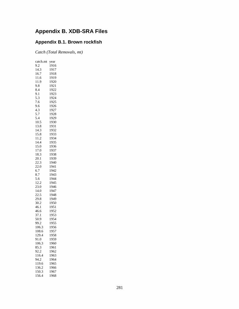
Appendix B. XDB-SRA Files Appendix B.1. Brown rockfish Catch (Total Removals, mt) catch.mt year 9.2 1916 14.3 1917 16.7 1918 11.6 1919 11.9 1920 9.8 1921 8.4 1922 9.1 1923 5.3 1924 7.6 1925 9.6 1926 4.3 1927 5.7 1928 5.4 1929 10.5 1930 13.8 1931 14.3 1932 15.8 1933 11.2 1934 14.4 1935 15.0 1936 17.0 1937 18.3 1938 20.1 1939 22.3 1940 22.0 1941 6.7 1942 8.7 1943 5.6 1944 12.2 1945 23.0 1946 14.0 1947 22.5 1948 29.8 1949 30.2 1950 46.1 1951 46.6 1952 37.1 1953 50.9 1954 99.2 1955 106.3 1956 108.6 1957 129.4 1958 91.0 1959 106.3 1960 85.3 1961 92.2 1962 116.4 1963 94.2 1964 119.6 1965 136.2 1966 150.3 1967 156.4 1968

281

126.9 1969 161.5 1970 161.2 1971 212.7 1972 310.4 1973 360.0 1974 313.7 1975 334.4 1976 284.8 1977 202.7 1978 196.3 1979 412.8 1980 141.2 1981 260.3 1982 139.6 1983 237.2 1984 217.6 1985 267.1 1986 190.2 1987 319.6 1988 213.3 1989 172.9 1990 170.4 1991 142.1 1992 137.8 1993 76.1 1994 76.6 1995 106.8 1996 154.3 1997 98.3 1998 125.8 1999 101.5 2000 151.8 2001 94.5 2002 169.3 2003 58.2 2004 100.4 2005 89.2 2006 76.1 2007 72.6 2008 84.9 2009 97.0 2010 112.7 2011 94.7 2012 101.5 2013 # avg. 2010-2012 101.5 2014 # avg. 2010-2012 151.3 2015 # 40-10 adjusted catch, Pstar 0.45

282

Central CA CPFV Onboard Observer Index for Brown Rockfish year index logSD 1988 0.34239806 0.200382572 1989 0.32699359 0.180369023 1990 0.37656108 0.323948708 1991 0.41192106 0.455332767 1992 0.26781914 0.18660012 1993 0.29231143 0.25586476 1994 0.19116646 0.241869417 1995 0.32258103 0.238588218 1996 0.2601924 0.210312235 1997 0.1564559 0.200791654 1998 0.3721465 0.166187027 1999 0.13321081 0.513543014 2001 0.20608263 0.251495715 2002 0.09451003 0.34102123 2003 0.28144315 0.140344282 2004 0.31042538 0.129845183 2005 0.3096305 0.160046124 2006 0.51170771 0.127220295 2007 0.44385928 0.140763331 2008 0.29668747 0.203527786 2009 0.41620333 0.188783909 2010 0.35673849 0.116790411 2011 0.31699517 0.133431094 Southern CA CPFV Onboard Observer Index for Brown Rockfish year index logSD 1999 0.008914224 0.364606051 2000 0.005468816 0.401970843 2001 0.007865838 0.388155065 2002 0.02288711 0.210903267 2003 0.029912146 0.202572065 2004 0.019347095 0.241814764 2005 0.036638665 0.164697497 2006 0.085673157 0.123720645 2007 0.054971952 0.138601482 2008 0.081503421 0.119140761 2009 0.064696945 0.108417821 2010 0.08261015 0.112313676 2011 0.057716836 0.153526767 Central CA RecFIN Dockside Observer Index for Brown Rockfish year index logSD 1980 0.19340974 0.390437534 1981 0.09921671 0.52650861 1983 1.02295082 0.59012895 1984 0.12287234 0.569648147 1985 0.1421709 0.237359448 1986 0.39063355 0.30293007 1987 0.24796126 0.556820189 1988 0.33268108 0.935793124 1989 0.04758128 0.528850078 1993 0.14525133 0.727062236 1994 0.03639847 0.826638216 1996 0.08476253 0.252058272 1999 0.1369259 0.51629563 2000 0.09565217 0.436424928 2001 0.11541137 0.245042617 2002 0.06203304 0.217282044 2003 0.1604449 0.276676775

283

Southern CA RecFIN Dockside Observer Index for Brown Rockfish year index logSD 1980 0.020053821 0.523284 1981 0.021804458 0.9573383 1982 0.0353475 0.9598115 1983 0.010590486 0.5297299 1984 0.016735148 0.4476916 1985 0.009591447 0.4137208 1986 0.002267574 0.6843325 1988 0.006654568 0.4892862 1994 0.012811162 0.8014592 1996 0.003915139 0.717811 1998 0.007886473 0.4537797 1999 0.019178731 0.5172163 2000 0.022102944 0.6066723 2001 0.04481261 0.5026588 2002 0.019180274 0.4161548 2003 0.030154548 0.5445968 XDB-SRA Control File for Brown Rockfish sci.name Sebastes crameri common.name Brown Rockfish species.code BRWN age.mat 4 delta.yr 2000 current.yr 2013 DBSRA.OFL.yr 2015 M.est 0.14 SD.lnM 0.4 FMSYtoMratio 0.97 SD.FMSYtoMratio 0.46 Delta 0.7 SD.Delta 0.2 DeltaLowerBound 0.01 DeltaUpperBound 0.99 BMSYtoB0ratio 0.4 SD.BMSYtoB0ratio 0.15 BMSYtoB0LowerBound 0.05 BMSYtoB0UpperBound 0.95 random.seed 1705 Appendix B.2. China rockfish, South of Cape Mendocino Catch (Total Removals, mt) catch.mt year 6.5 1916 10.1 1917 11.9 1918 8.2 1919 8.4 1920 6.9 1921 6.0 1922 6.5 1923 3.7 1924 4.7 1925 7.5 1926 6.4 1927 8.2 1928 7.2 1929 10.0 1930 5.1 1931

284

11.5 1932 5.5 1933 10.1 1934 9.5 1935 9.8 1936 9.6 1937 7.7 1938 5.4 1939 5.5 1940 5.1 1941 2.8 1942 3.8 1943 2.1 1944 2.7 1945 5.3 1946 4.6 1947 9.4 1948 12.4 1949 11.3 1950 13.8 1951 12.1 1952 10.6 1953 11.0 1954 12.6 1955 13.9 1956 14.2 1957 22.7 1958 18.1 1959 15.1 1960 14.7 1961 12.6 1962 16.0 1963 10.1 1964 17.0 1965 18.9 1966 24.3 1967 21.1 1968 23.2 1969 37.3 1970 27.1 1971 39.2 1972 50.3 1973 49.5 1974 48.0 1975 52.1 1976 47.8 1977 33.3 1978 44.4 1979 59.2 1980 36.3 1981 47.0 1982 24.2 1983 25.0 1984 30.6 1985 43.9 1986 59.3 1987 42.9 1988 38.3 1989 36.4 1990 40.4 1991 49.3 1992 41.7 1993

285

61.9 1994 46.6 1995 33.9 1996 39.0 1997 19.0 1998 21.2 1999 20.6 2000 19.1 2001 18.1 2002 17.6 2003 9.9 2004 15.9 2005 12.8 2006 13.5 2007 15.3 2008 20.3 2009 18.9 2010 15.7 2011 13.6 2012 16.1 2013 # avg. 2010-2012 16.1 2014 # avg. 2010-2012 50.4 2015 # 40-10 adjusted catch, Pstar 0.45 Southern and Central CA RecFIN Dockside Observer Index for China Rockfish year index logSD 1980 0.0327 0.404235796 1981 0.0498 0.747530915 1983 0.0592 0.421544477 1984 0.0137 0.514363007 1985 0.0253 0.31911839 1986 0.0496 0.330684643 1987 0.0486 0.428309101 1988 0.0584 0.363905742 1989 0.0669 0.409595198 1993 0.0143 0.630114726 1994 0.018 0.412401021 1995 0.1076 0.232772535 1996 0.0449 0.148121036 1999 0.0302 0.23338366 2000 0.0304 0.26246385 2001 0.0698 0.206670473 2002 0.0801 0.181523255 2003 0.0607 0.167036666 Central CA CPFV Onboard Observer Index for China Rockfish year index logSD 1988 0.0512 0.169 1989 0.052 0.168 1990 0.117 0.225 1991 0.0733 0.293 1992 0.0409 0.175 1993 0.0461 0.186 1994 0.0731 0.147 1995 0.0456 0.191 1996 0.0522 0.157 1997 0.0375 0.188 1998 0.0186 0.228 1999 0.0429 0.294 2001 0.0328 0.273 2002 0.0544 0.268 2003 0.0671 0.184 2004 0.0594 0.167

286

2005 0.0565 0.237 2006 0.0518 0.214 2007 0.0737 0.183 2008 0.0674 0.193 2009 0.1014 0.178 2010 0.0878 0.171 2011 0.064 0.166 XDB-SRA Control File for China Rockfish, South of Cape Mendocino sci.name Sebastes nebulosus common.name China Rockfish species.code CHNA age.mat 5 current.yr 2013 delta.yr 2000 DBSRA.OFL.yr 2013 M.est 0.06 SD.lnM 0.4 FMSYtoMratio 0.97 SD.FMSYtoMratio 0.46 Delta 0.7 SD.Delta 0.2 DeltaLowerBound 0.01 DeltaUpperBound 0.99 BMSYtoB0ratio 0.4 SD.BMSYtoB0ratio 0.15 BMSYtoB0LowerBound 0.05 BMSYtoB0UpperBound 0.95 random.seed 824

287

Appendix B.3. China rockfish, North of Cape Mendocino Catch (Total Removals, mt) catch.mt year 0.0 1916 0.0 1917 0.0 1918 0.0 1919 0.0 1920 0.0 1921 0.0 1922 0.0 1923 0.0 1924 0.0 1925 0.0 1926 0.0 1927 0.0 1928 0.1 1929 0.1 1930 0.1 1931 0.0 1932 0.1 1933 0.8 1934 0.6 1935 1.0 1936 0.8 1937 2.6 1938 4.7 1939 3.0 1940 1.0 1941 0.8 1942 0.4 1943 0.4 1944 0.5 1945 0.6 1946 0.3 1947 0.5 1948 0.4 1949 0.3 1950 0.3 1951 0.3 1952 0.1 1953 0.1 1954 0.2 1955 0.2 1956 0.4 1957 0.1 1958 0.1 1959 0.1 1960 0.3 1961 0.3 1962 0.5 1963 0.5 1964 0.9 1965 0.9 1966 1.4 1967 1.5 1968 2.5 1969 2.0 1970 3.0 1971 3.5 1972

288

4.5 1973 5.7 1974 4.2 1975 5.0 1976 5.2 1977 7.2 1978 9.9 1979 10.7 1980 10.4 1981 10.6 1982 9.1 1983 8.9 1984 6.9 1985 7.3 1986 8.7 1987 7.9 1988 11.9 1989 17.6 1990 10.4 1991 15.6 1992 12.6 1993 17.5 1994 18.0 1995 15.8 1996 22.0 1997 27.3 1998 35.5 1999 22.0 2000 28.0 2001 29.0 2002 16.5 2003 12.0 2004 9.4 2005 11.1 2006 15.4 2007 16.3 2008 15.1 2009 11.8 2010 16.4 2011 17.3 2012 15.2 2013 # avg. 2010-2012 15.2 2014 # avg. 2010-2012 6.2 2015 # 40-10 adjusted catch, Pstar 0.45

289

Northern CA and OR RecFIN Dockside Observer Index for China Rockfish year index logSD 1980 0.1014 0.515 1981 0.059 0.263 1982 0.0441 0.642 1983 0.0193 0.65 1984 0.0192 0.366 1985 0.06 0.373 1986 0.0242 0.533 1987 0.0684 0.47 1988 0.0407 0.29 1989 0.031 0.358 1993 0.0437 0.3 1994 0.0404 0.257 1995 0.0252 0.291 1996 0.0244 0.332 1997 0.0374 0.245 1998 0.0277 0.222 1999 0.0423 0.179 2000 0.0431 0.272 2001 0.0138 0.464 2002 0.0156 0.34 2003 0.0271 0.472 OR CPFV Onboard Observer Index for China Rockfish year index logSD 2001 0.0299 0.268 2003 0.0298 0.239 2004 0.019 0.335 2005 0.0135 0.35 2006 0.0177 0.291 2007 0.0346 0.212 2008 0.0176 0.275 2009 0.0287 0.248 2010 0.007 0.508 2011 0.0217 0.444 2012 0.0335 0.269 XDB-SRA Control File for China Rockfish, North of Cape Mendocino sci.name Sebastes nebulosus common.name China Rockfish species.code CHNA age.mat 5 current.yr 2013 delta.yr 2000 DBSRA.OFL.yr 2013 M.est 0.06 SD.lnM 0.4 FMSYtoMratio 0.97 SD.FMSYtoMratio 0.46 Delta 0.7 SD.Delta 0.2 DeltaLowerBound 0.01 DeltaUpperBound 0.99 BMSYtoB0ratio 0.4 SD.BMSYtoB0ratio 0.15 BMSYtoB0LowerBound 0.05 BMSYtoB0UpperBound 0.95 random.seed 824

290

Appendix B.4. Copper rockfish, South of Point Conception Catch (Total Removals, mt) catch.mt year 0.1 1916 0.2 1917 0.2 1918 0.1 1919 0.1 1920 0.1 1921 0.1 1922 0.1 1923 0.2 1924 0.2 1925 0.3 1926 0.2 1927 0.2 1928 0.2 1929 0.3 1930 0.3 1931 0.3 1932 0.2 1933 0.3 1934 0.6 1935 0.4 1936 1.2 1937 0.7 1938 0.5 1939 0.5 1940 0.6 1941 0.1 1942 0.2 1943 0.1 1944 0.2 1945 0.2 1946 0.7 1947 1.8 1948 2.3 1949 3.2 1950 5.9 1951 4.5 1952 4.1 1953 8.6 1954 16.7 1955 18.3 1956 10.8 1957 10.9 1958 5.9 1959 6.8 1960 9.7 1961 6.6 1962 7.0 1963 11.8 1964 17.4 1965 43.8 1966 50.7 1967 59.3 1968 47.0 1969 69.6 1970 66.8 1971 92.2 1972

291

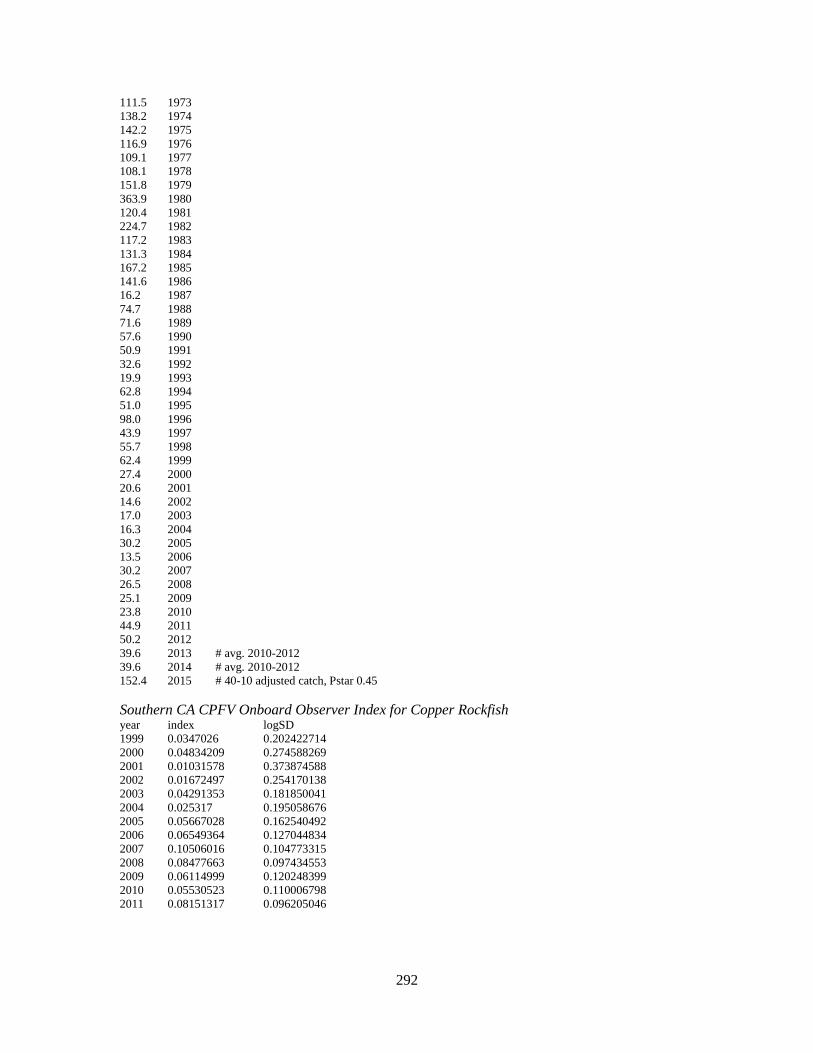
111.5 1973 138.2 1974 142.2 1975 116.9 1976 109.1 1977 108.1 1978 151.8 1979 363.9 1980 120.4 1981 224.7 1982 117.2 1983 131.3 1984 167.2 1985 141.6 1986 16.2 1987 74.7 1988 71.6 1989 57.6 1990 50.9 1991 32.6 1992 19.9 1993 62.8 1994 51.0 1995 98.0 1996 43.9 1997 55.7 1998 62.4 1999 27.4 2000 20.6 2001 14.6 2002 17.0 2003 16.3 2004 30.2 2005 13.5 2006 30.2 2007 26.5 2008 25.1 2009 23.8 2010 44.9 2011 50.2 2012 39.6 2013 # avg. 2010-2012 39.6 2014 # avg. 2010-2012 152.4 2015 # 40-10 adjusted catch, Pstar 0.45 Southern CA CPFV Onboard Observer Index for Copper Rockfish year index logSD 1999 0.0347026 0.202422714 2000 0.04834209 0.274588269 2001 0.01031578 0.373874588 2002 0.01672497 0.254170138 2003 0.04291353 0.181850041 2004 0.025317 0.195058676 2005 0.05667028 0.162540492 2006 0.06549364 0.127044834 2007 0.10506016 0.104773315 2008 0.08477663 0.097434553 2009 0.06114999 0.120248399 2010 0.05530523 0.110006798 2011 0.08151317 0.096205046

292

Southern CA RecFIN Dockside Observer Index for Copper Rockfish year index logSD 1980 0.08374128 0.385044159 1981 0.04934085 0.3743977 1982 0.0291001 0.619788449 1983 0.11078686 0.604208127 1984 0.09522736 0.444209452 1985 0.04527815 0.424033134 1986 0.08328542 0.459150935 1988 0.16267752 0.613231574 1993 0.08325661 0.529162455 1994 0.08350039 0.980984905 1995 0.06296092 0.61486449 1996 0.13282901 0.323678637 1997 0.07748774 0.960291868 1998 0.0885108 0.40754817 1999 0.1479035 0.254902986 2000 0.09307187 0.456695668 2001 0.08665951 0.383998641 2002 0.07425175 0.232851561 2003 0.1612675 0.409675572 XDB-SRA Control File for Copper Rockfish, South of Point Conception sci.name Sebastes caurinus common.name Copper Rockfish species.code COPP age.mat 6 delta.yr 2000 current.yr 2013 DBSRA.OFL.yr 2013 M.est 0.09 SD.lnM 0.4 FMSYtoMratio 0.97 SD.FMSYtoMratio 0.46 Delta 0.7 SD.Delta 0.2 DeltaLowerBound 0.01 DeltaUpperBound 0.99 BMSYtoB0ratio 0.4 SD.BMSYtoB0ratio 0.15 BMSYtoB0LowerBound 0.05 BMSYtoB0UpperBound 0.95 random.seed 824 Appendix B.5. Copper rockfish, North of Point Conception Catch (Total Removals, mt) catch.mt year 4.1 1916 6.4 1917 7.8 1918 5.1 1919 5.2 1920 4.5 1921 3.8 1922 4.0 1923 2.7 1924 4.0 1925 5.1 1926 3.8 1927 5.4 1928

293

6.4 1929 9.3 1930 11.4 1931 11.9 1932 12.3 1933 12.2 1934 15.6 1935 16.4 1936 19.2 1937 18.4 1938 16.5 1939 21.3 1940 20.4 1941 10.1 1942 11.0 1943 15.6 1944 30.8 1945 39.4 1946 18.8 1947 32.7 1948 34.7 1949 39.6 1950 54.4 1951 45.6 1952 36.5 1953 47.2 1954 52.7 1955 60.4 1956 58.6 1957 99.5 1958 80.6 1959 68.7 1960 51.5 1961 64.0 1962 79.8 1963 71.2 1964 105.8 1965 121.9 1966 129.7 1967 137.2 1968 147.7 1969 182.4 1970 171.2 1971 217.7 1972 249.2 1973 274.2 1974 270.3 1975 299.5 1976 309.0 1977 285.0 1978 295.8 1979 117.4 1980 400.4 1981 220.6 1982 175.6 1983 144.8 1984 160.0 1985 124.7 1986 102.1 1987 96.9 1988 108.1 1989 123.3 1990

294

130.1 1991 152.4 1992 149.4 1993 83.7 1994 70.6 1995 89.3 1996 91.6 1997 60.8 1998 54.6 1999 39.8 2000 35.8 2001 28.2 2002 28.3 2003 23.2 2004 41.2 2005 43.1 2006 48.6 2007 38.9 2008 45.7 2009 34.4 2010 35.6 2011 44.9 2012 38.3 2013 # avg. 2010-2012 38.3 2014 # avg. 2010-2012 132.3 2015 # 40-10 adjusted catch, Pstar 0.45 Central CA CPFV Onboard Observer Index for Copper Rockfish year index logSD 1988 0.0397 0.142 1989 0.0597 0.119 1990 0.0724 0.2 1991 0.0468 0.223 1992 0.0686 0.121 1993 0.0697 0.125 1994 0.0495 0.133 1995 0.0603 0.125 1996 0.0576 0.121 1997 0.0604 0.127 1998 0.0552 0.152 1999 0.0403 0.409 2001 0.1001 0.219 2002 0.0545 0.374 2003 0.0736 0.199 2004 0.0939 0.117 2005 0.1555 0.124 2006 0.1497 0.11 2007 0.1309 0.117 2008 0.0764 0.164 2009 0.0705 0.179 2010 0.137 0.113 2011 0.1029 0.124 Central/Northern CA and OR RecFIN Dockside Observer Index for Copper Rockfish year index logSD 1980 0.0344263 0.437861772 1981 0.11580617 0.38704024 1982 0.04417949 0.451436183 1983 0.11141602 0.348087994 1984 0.12819123 0.449678658 1985 0.0555466 0.337609966 1986 0.09774667 0.219435546 1987 0.02798718 1.155683336

295

1988 0.02755241 0.359211559 1989 0.08905342 0.250402589 1993 0.06030649 0.280590726 1994 0.05983713 0.285738388 1995 0.02109752 0.471002191 1996 0.05212757 0.125912001 1997 0.0479666 0.308124197 1998 0.04245647 0.385537868 1999 0.05072293 0.153286935 2000 0.05042611 0.316376639 2001 0.041476 0.219157638 2002 0.03737898 0.303376218 2003 0.02508151 0.209186744 OR CPFV Onboard Observer Index for Copper Rockfish year index logSD 2001 0.0264 0.34 2003 0.0147 0.357 2004 0.0118 0.406 2005 0.0387 0.301 2006 0.0384 0.257 2007 0.0304 0.234 2008 0.0149 0.316 2009 0.0316 0.284 2010 0.0406 0.297 2011 0.0137 0.484 2012 0.023 0.354 XDB-SRA Control File for Copper Rockfish, North of Point Conception sci.name Sebastes caurinus common.name Copper Rockfish species.code COPP age.mat 6 delta.yr 2000 current.yr 2013 DBSRA.OFL.yr 2013 M.est 0.09 SD.lnM 0.4 FMSYtoMratio 0.97 SD.FMSYtoMratio 0.46 Delta 0.7 SD.Delta 0.2 DeltaLowerBound 0.01 DeltaUpperBound 0.99 BMSYtoB0ratio 0.4 SD.BMSYtoB0ratio 0.15 BMSYtoB0LowerBound 0.05 BMSYtoB0UpperBound 0.95 random.seed 824

296

Appendix C. Partitioning OFLs for brown and copper rockfish During the STAR Panel, the STAT presented regional models for brown rockfish and copper rockfish (north and south of Point Conception). The Panel recommended that the OFL for brown rockfish be based on the coastwide model, partitioned into areas north and south of Point Conception based on the regional models. The Panel considered the regional models for copper rockfish to be adequate for OFL determination. However, the assessments for brown rockfish (coastwide) and copper rockfish (north of Point Conception, CA) span the boundary between the PFMC’s northern and southern rockfish complexes (40° 10′ N lat., roughly near Cape Mendocino). This appendix describes possible methods to partition the OFL estimate into northern and southern components. When regional assessments are not available, partitioning of OFLs would ideally involve taking the product of density and habitat area to arrive at an estimate of abundance (or relative abundance) in each management area. The STAT considered using estimates of habitat area derived from recreational catch observations (see section 2.1.6.2), combined with a proxy for density (CPUE) derived from recreational catch data. In the end, this approach was not possible for copper rockfish because the STAT did not have CPUE and habitat information off Washington, which is needed to create a complete estimate of relative abundance north of Cape Mendocino. The density of brown rockfish in Washington is effectively zero, but catch rates north of Cape Mendocino are so low that an analysis based on detailed habitat area estimates and catch rates is unlikely to differ significantly from a simpler, catch-based approach. Appendix C.1. Brown rockfish To partition the OFL for brown rockfish, we used regional assessments to estimate median vulnerable biomass levels in 2015 assuming recent average catch in 2013-14. Vulnerable biomass estimates in 2015 were 381.6 mt south of Point Conception and 1082.3 mt north of Point Conception. Approximately 26.1% (381.6 / (381.6+1082.3)) of coastwide brown rockfish biomass in 2013 is south of Point Conception. Dick and MacCall (2010, their Table 65) developed a catch-based allocation of OFL, finding that 2.6% of coastwide brown rockfish biomass is north of Cape Mendocino. The remaining percentage (biomass in central California) is therefore 71.3% of coastwide biomass. Applying these percentages to the median OFL in 2015 from the coastwide brown rockfish assessment (164 mt) provides regional estimates of OFL (Table B1). Table B1. Brown rockfish OFLs for 2015, by region

% of coastwide OFL OFL (mt) Southern CA 26.1% 42.8 Central CA 71.3% 116.9 South of 40° 10′ N lat. (South + Central) 97.4% 159.7 North of 40° 10′ N lat. 2.6% 4.3

297

Appendix C.2. Copper rockfish We apply a similar method to that used for brown rockfish (above), but based on regional model OFLs (per the STAR Panel’s recommendation). We estimated median vulnerable biomass levels in 2015 assuming recent average catch in 2013-14. Vulnerable biomass estimates in 2015 were 1420 mt south of Point Conception and 1691.2 mt north of Point Conception. Approximately 45.6% (1420 / (1420+1691.2)) of coastwide copper rockfish biomass in 2013 is south of Point Conception. The large fraction of biomass estimated for southern California is influenced by the recent increases in biomass in that area, relative to the central/northern stock. Dick and MacCall (2010, their Table 65) developed a catch-based allocation of OFL, finding that 15.5% of coastwide copper rockfish biomass is north of Cape Mendocino. The remaining percentage (biomass in central California) is therefore 38.6% of coastwide biomass. Using the percentages for central California (38.9%) and the area north of Cape Mendocino (15.5%), we estimate that 28.5% (15.5 / (15.5+38.9)) of the central/northern copper rockfish OFL estimate for 2015 should be allocated north of Cape Mendocino (Table B2). Table B2. Copper rockfish OFLs ,by region, using catch-based allocation method

Source 2015 OFL (mt) South of Conception model median estimate 165 North of Conception model median estimate 144 Coastwide (sum of regional models) 309 North of 40° 10′ N lat. Northern OFL * 0.285 41.0 South of 40° 10′ N lat. 309 – 41 268

298

Documents

Data-moderate stock assessments for brown, China, copper