Embed Size (px)
Citation preview

DataMiningandPa+ernRecogni1on
SalvatoreOrlando,AndreaTorsello,FilippoBergamasco
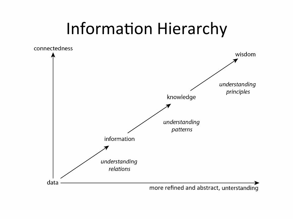
Informa1onHierarchy
morerefinedandabstract,
A(Face1ous)Example
• Data– 37º,38.5º,39.3º,40º,…
• Informa1on– Hourlybodytemperature:37º,38.5º,39.3º,40º,…
• Knowledge– Ifyouhaveatemperatureabove37º,youmostlikelyhaveafever
• Wisdom(ac1onable)– Ifyouhaveafeveranddon’tfeelwell,goseeadoctor
ContentofCHresources
• SomeCHcontentcanbestoredlosslessindigitallibrariesanddatabases– textdocuments,digitalphotos,music,etc
• Digitaliza1onmaycausealossofinforma1on– e.g.,imageresolu1on,audio/videoquality
• Inmostcasescontentisnot“digital”andsurrogatesareused– imagesforpain1ngs,manuscripts,ar1facts– 3Dmodelsforbuildings,sculptures,etc.

DATA,FEATURES

What is Data we Analyze? • Collection of data objects and
their attributes
• An attribute is a property or characteristic of an object – Examples: eye color of a person,
temperature of a room, etc. – Attribute is also known as
variable, field, characteristic, or feature
• A collection of attributes describes an object – Object is also known as record,
point, case, sample, entity, or instance
• Attribute values – numbers or symbols assigned to
an attribute
Tid Refund Marital Status
Taxable Income Cheat
1 Yes Single 125K No
2 No Married 100K No
3 No Single 70K No
4 Yes Married 120K No
5 No Divorced 95K Yes
6 No Married 60K No
7 Yes Divorced 220K No
8 No Single 85K Yes
9 No Married 75K No
10 No Single 90K Yes 10
Attributes
Objects

Unstructured Raw Data
• Consider a digital text or a digital image – We cannot recognize a record structure (a collection of a
fixed number of data, with metadata describing them) • A digital text is a list of characters encoded in bysomekindofnumericalencodingsystem(e.g.,ASCII)
• A digital image is a numeric representation of a two-dimensional image – Raster images have a finite set of digital values, called
picture elements or pixels (rows × columns) – Pixels hold quantized values that represent the brightness
of a given color at any specific point.

INFORMATIONRETRIEVAL

Digitaldatadeluge• Plaintext(documentsand
por1onsthereof)• XMLandstructured
documents• Webdocs• Images• Audio(soundeffects,songs,
etc.)• Video• Graphs/networks• Sourcecode• Apps/Webservices
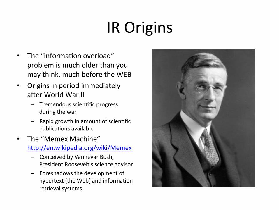
IROrigins• The“informa1onoverload”
problemismucholderthanyoumaythink,muchbeforetheWEB
• OriginsinperiodimmediatelyauerWorldWarII
– Tremendousscien1ficprogressduringthewar
– Rapidgrowthinamountofscien1ficpublica1onsavailable
• The“MemexMachine”h+p://en.wikipedia.org/wiki/Memex
– ConceivedbyVannevarBush,PresidentRoosevelt'sscienceadvisor
– Foreshadowsthedevelopmentofhypertext(theWeb)andinforma1onretrievalsystems
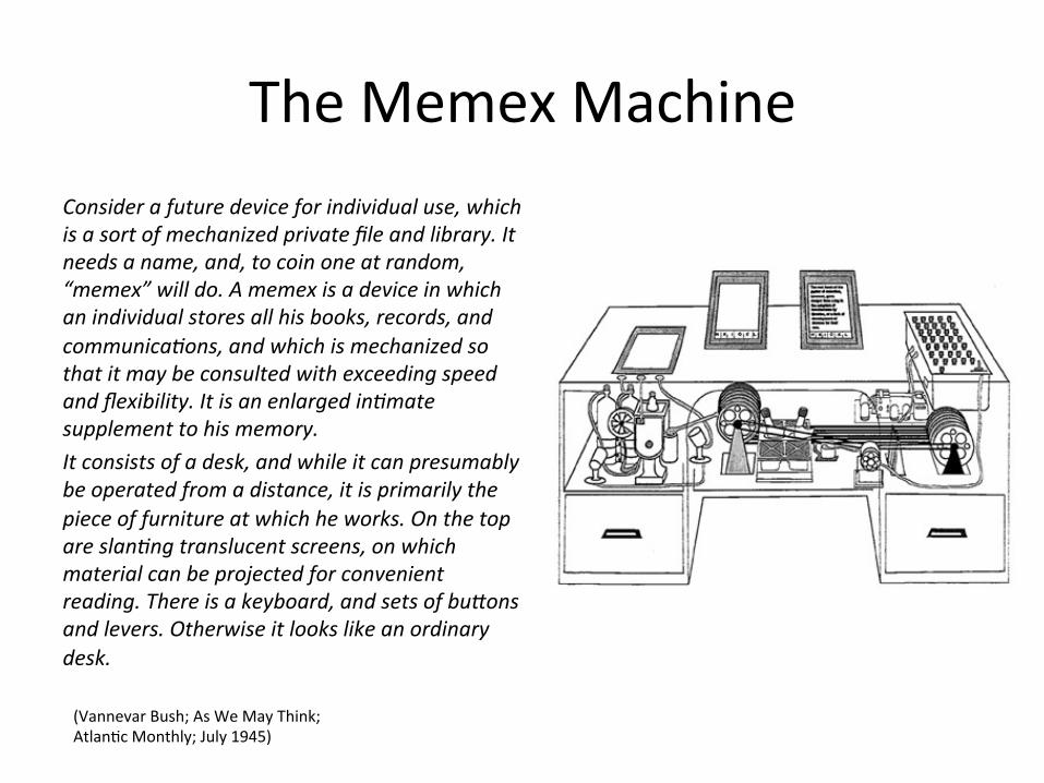
TheMemexMachineConsiderafuturedeviceforindividualuse,whichisasortofmechanizedprivatefileandlibrary.Itneedsaname,and,tocoinoneatrandom,“memex”willdo.Amemexisadeviceinwhichanindividualstoresallhisbooks,records,andcommunicaAons,andwhichismechanizedsothatitmaybeconsultedwithexceedingspeedandflexibility.ItisanenlargedinAmatesupplementtohismemory.Itconsistsofadesk,andwhileitcanpresumablybeoperatedfromadistance,itisprimarilythepieceoffurnitureatwhichheworks.OnthetopareslanAngtranslucentscreens,onwhichmaterialcanbeprojectedforconvenientreading.Thereisakeyboard,andsetsofbuGonsandlevers.Otherwiseitlookslikeanordinarydesk. (VannevarBush;AsWeMayThink;Atlan1cMonthly;July1945)

TheCentralProbleminIRInforma1onSeeker Authors/Contentproviders
Concepts Concepts
QueryTerms DocumentTerms
Dotheserepresentthesameconcepts?
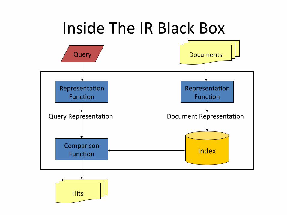
InsideTheIRBlackBoxDocumentsQuery
Hits
Representa1onFunc1on
Representa1onFunc1on
QueryRepresenta1on DocumentRepresenta1on
ComparisonFunc1on Index

WebSearches• WSE
– indexbillionsofpages– Answerhundredsofmillions
ofqueriesperday– Inlessthan0,5sec.perquery
• Users– Submitshortqueries(onavg.
2.5terms),ouenwithorthographicerrors
– ExpecttoreceivethemostrelevantresultsoftheWeb
– Inablinkofeye
24
Featureextrac1on• Featureextrac1onisconcernedwith
– Represen1ngeachunstructureddataelementintermsofarecord/vectorofalphanumericvalues,alsocalledfeatures
– Itrequirestomanipulaterawdatatoextractfeatures• Whyisitneededtorepresentdataassetsoffeature?– ThereasonisthatmanyInforma1onretrieval,Datamining,andPa+ernrecogni1onmethodsneedtousetheserepresenta1onstoapplytheiralgorithms
Howdowerepresenttext?
• Howdowerepresentthecomplexi1esoflanguage?– Keepinginmindthatcomputersdon’t“understand”documentsorqueries
• Simple,yeteffec1veapproach:“bagofwords”– Treatallthewordsinadocumentasindextermsforthatdocument
– Assigna“weight”toeachtermbasedonits“importance”
– Disregardorder,structure,meaning,etc.ofthewords
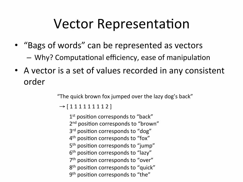
VectorRepresenta1on• “Bagsofwords”canberepresentedasvectors
– Why?Computa1onalefficiency,easeofmanipula1on
• Avectorisasetofvaluesrecordedinanyconsistentorder
“Thequickbrownfoxjumpedoverthelazydog’sback”
→[111111112]
1stposi1oncorrespondsto“back”2ndposi1oncorrespondsto“brown”3rdposi1oncorrespondsto“dog”4thposi1oncorrespondsto“fox”5thposi1oncorrespondsto“jump”6thposi1oncorrespondsto“lazy”7thposi1oncorrespondsto“over”8thposi1oncorrespondsto“quick”9thposi1oncorrespondsto“the”
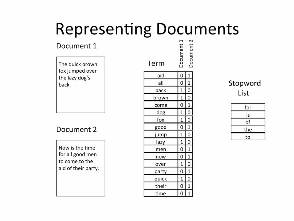
Represen1ngDocuments
Thequickbrownfoxjumpedoverthelazydog’sback.
Document1
Document2
Nowisthe1meforallgoodmentocometotheaidoftheirparty.
the
isfor
to
of
quick
brown
fox
over
lazy
dog
back
now
1me
all
good
men
come
jump
aid
their
party
00110110110010100
11001001001101011
Term Do
cumen
t1
Documen
t2
StopwordList

Featureextrac1ontoRepresentTextDocuments
Thequickbrownfoxjumpedoverthelazydog’sback.
Document1
Document2
Nowisthe1meforallgoodmentocometotheaidoftheirparty.
the
isfor
to
of
quick
brown
fox
over
lazy
dog
back
now
1me
all
good
men
come
jump
aid
their
party
00110110110010100
11001001001101011
Term Do
cumen
t1
Documen
t2
StopwordList
DocumentVector,whereeach
featurerepresentsthenumberofoccurrencesofeachterm

BasicIRModels• Booleanmodel
– Basedontheno1onofsets– Documentsareretrievedonlyiftheysa1sfyBooleancondi1onsspecifiedinthequery
– Doesnotimposearankingonretrieveddocuments– Exactmatch
• Vectorspacemodel– Basedongeometry,theno1onofvectorsinhighdimensionalspace
– Documentsarerankedbasedontheirsimilaritytothequery(rankedretrieval)
– Best/par1almatch
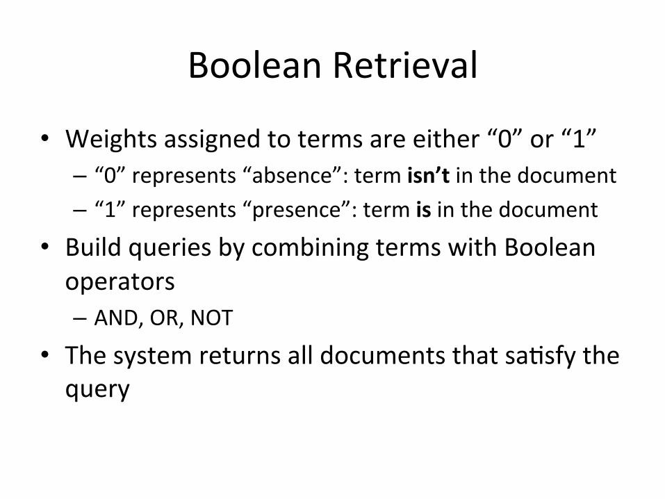
BooleanRetrieval
• Weightsassignedtotermsareeither“0”or“1”– “0”represents“absence”:termisn’tinthedocument– “1”represents“presence”:termisinthedocument
• BuildqueriesbycombiningtermswithBooleanoperators– AND,OR,NOT
• Thesystemreturnsalldocumentsthatsa1sfythequery

BooleanViewofaCollec1on
quick
brown
fox
over
lazy
dog
back
now
1me
all
good
men
come
jump
aid
their
party
00110000010010110
01001001001100001
Term
Doc1
Doc2
00110110110010100
11001001001000001
Doc3
Doc4
00010110010010010
01001001000101001
Doc5
Doc6
00110010010010010
10001001001111000
Doc7
Doc8
Eachcolumnrepresentstheviewofapar1culardocument:Whattermsarecontainedinthisdocument?
Eachrowrepresentstheviewofapar1cularterm:Whatdocumentscontainthisterm?
Toexecuteaquery,pickoutrowscorrespondingtoquerytermsandthenapplylogictableofcorrespondingBooleanoperator

AND/OR/NOT
Apple Pear
Alldocuments
Orange
(AppleandPear)orOrange

LogicTables
AORB
AANDB ANOTB
NOTB
0 1
1 1
0 1
0
1
AB
(=AANDNOTB)
0 0
0 1
0 1
0
1
AB
0 0
1 0
0 1
0
1
AB
1 0
0 1B
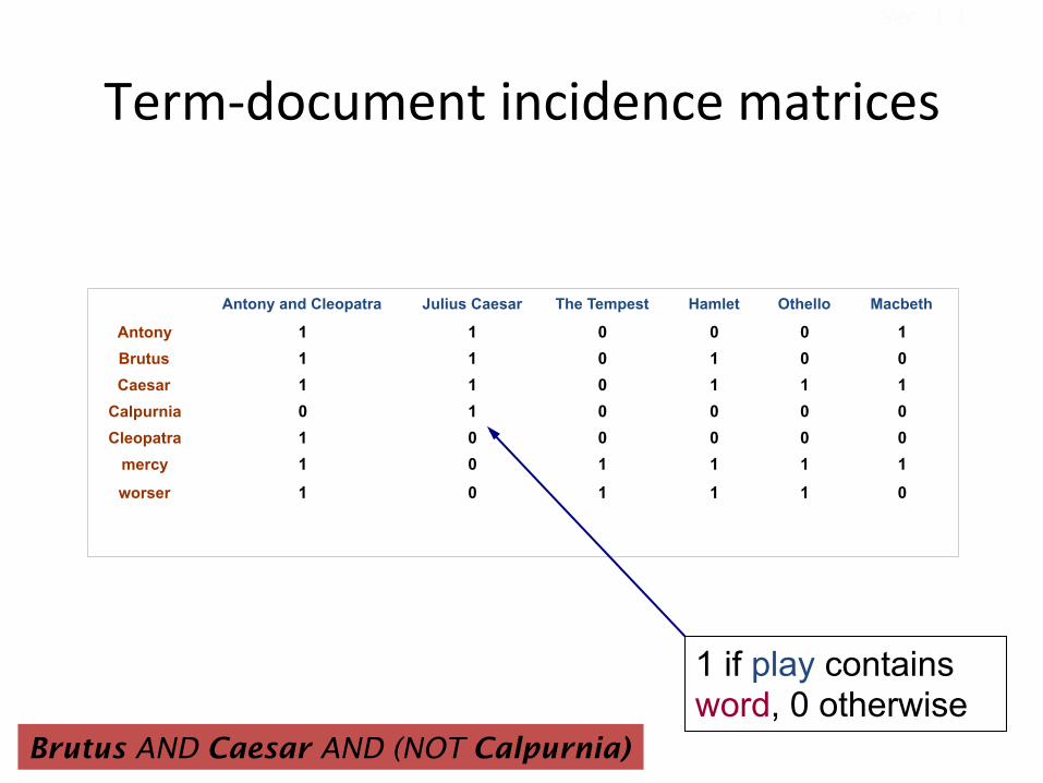
Term-documentincidencematrices
Antony and Cleopatra Julius Caesar The Tempest Hamlet Othello Macbeth
Antony 1 1 0 0 0 1Brutus 1 1 0 1 0 0Caesar 1 1 0 1 1 1
Calpurnia 0 1 0 0 0 0Cleopatra 1 0 0 0 0 0
mercy 1 0 1 1 1 1worser 1 0 1 1 1 0
1 if play contains word, 0 otherwise
Brutus AND Caesar AND (NOT Calpurnia)
Sec. 1.1

Incidencevectors
• Sowehavea0/1vectorforeachterm.• Toanswerquery:takethevectorsforBrutus,CaesarandCalpurnia(complemented)èbitwiseAND.– 110100AND– 110111AND– 101111=– 100100
34
Sec. 1.1
Antony and Cleopatra Julius Caesar The Tempest Hamlet Othello Macbeth
Antony 1 1 0 0 0 1Brutus 1 1 0 1 0 0Caesar 1 1 0 1 1 1
Calpurnia 0 1 0 0 0 0Cleopatra 1 0 0 0 0 0
mercy 1 0 1 1 1 1worser 1 0 1 1 1 0
Brutus AND Caesar AND (NOT Calpurnia)
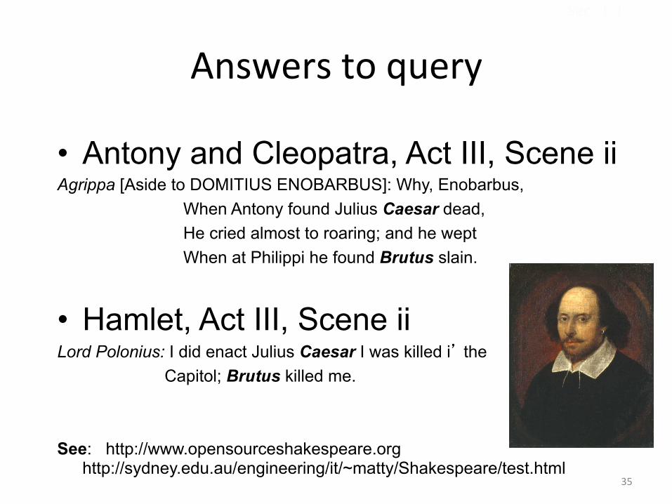
Answerstoquery
• Antony and Cleopatra,Act III, Scene ii Agrippa [Aside to DOMITIUS ENOBARBUS]: Why, Enobarbus, When Antony found Julius Caesar dead, He cried almost to roaring; and he wept When at Philippi he found Brutus slain.
• Hamlet, Act III, Scene ii Lord Polonius: I did enact Julius Caesar I was killed i� the Capitol; Brutus killed me. See: http://www.opensourceshakespeare.org
http://sydney.edu.au/engineering/it/~matty/Shakespeare/test.html 35
Sec. 1.1
WhyBooleanRetrievalWorks
• Booleanoperatorsapproximatenaturallanguage– Finddocumentsaboutagoodpartythatisnotover
• ANDcandiscoverrela1onshipsbetweenconcepts– goodparty
• ORcandiscoveralternateterminology– excellentparty,wildparty,etc.
• NOTcandiscoveralternatemeanings– Democra1cparty
See:h+p://sydney.edu.au/engineering/it/~ma+y/Shakespeare/test.htmlforasearchengineonShakespeareexploi1ngtheBooleanmodel
See:h+p://www.perunaenciclopediadantescadigitale.eu:8080/dantesearch/forasearchengineonDanteexploi1ngtheBooleanmodel
WhyBooleanRetrievalFails
• Naturallanguageiswaymorecomplex• AND“discovers”nonexistentrela1onships
– Termsindifferentsentences,paragraphs,…
• GuessingterminologyforORishard– good,nice,excellent,outstanding,awesome,…
• Guessingtermstoexcludeisevenharder!– Democra1cparty,partytoalawsuit,…

StrengthsandWeaknesses
Strengths• Precise,ifyouknowthe
rightstrategies• Precise,ifyouhaveanidea
ofwhatyou’relookingfor• Efficientforthecomputer
Weaknesses• UsersmustlearnBooleanlogic• Booleanlogicinsufficientto
capturetherichnessoflanguage
• Nocontroloversizeofresultset:eithertoomanydocumentsornone– Alldocumentsintheresultset
areconsidered“equallygood”– Doesnotfithugecollec1ons
• Nosupportforpar1almatches
RankedRetrieval• Orderdocumentsbyhow
likelytheyaretoberelevanttotheinforma1onneed– Presenthitsonescreenata1me
– Closertohowhumansthink:somedocumentsare“be+er”thanothers
– Closertouserbehavior:userscandecidewhentostopreading
– Fitsbe+erhugecollec1onsofdocuments
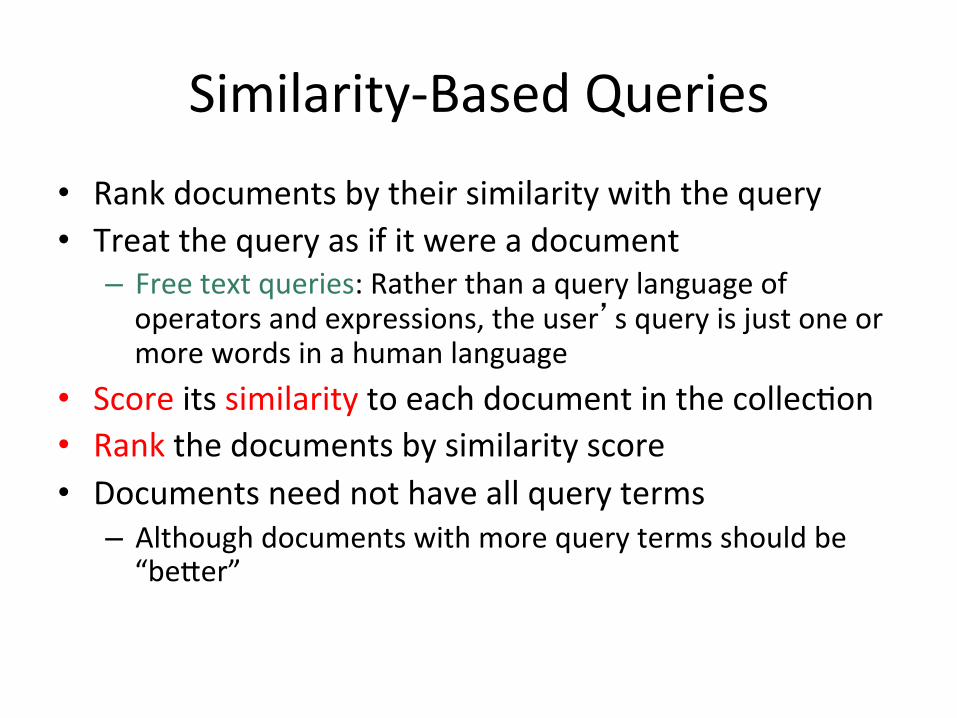
Similarity-BasedQueries• Rankdocumentsbytheirsimilaritywiththequery• Treatthequeryasifitwereadocument
– Freetextqueries:Ratherthanaquerylanguageofoperatorsandexpressions,theuser�squeryisjustoneormorewordsinahumanlanguage
• Scoreitssimilaritytoeachdocumentinthecollec1on• Rankthedocumentsbysimilarityscore• Documentsneednothaveallqueryterms
– Althoughdocumentswithmorequerytermsshouldbe“be+er”
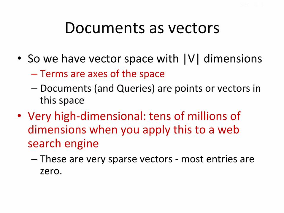
Documentsasvectors
• Sowehavevectorspacewith|V|dimensions– Termsareaxesofthespace– Documents(andQueries)arepointsorvectorsinthisspace
• Veryhigh-dimensional:tensofmillionsofdimensionswhenyouapplythistoawebsearchengine– Theseareverysparsevectors-mostentriesarezero.
Sec. 6.3

Queriesasvectors
• Keyidea1:Dothesameforqueries:representthemasvectorsinthespace
• Keyidea2:Rankdocumentsaccordingtotheirproximitytothequeryinthisspace
• proximity=similarityofvectors• proximity≈inverseofdistance
Sec. 6.3

Formalizingvectorspaceproximity
• Firstcut:distancebetweentwopoints– (=distancebetweentheendpointsofthetwovectors)
• Euclideandistance?• Euclideandistanceisabadidea...• ...becauseEuclideandistanceislargeforvectorsofdifferentlengths.
Sec. 6.3

Whydistanceisabadidea
TheEuclideandistancebetweenqandd2islargeeventhoughthedistribu1onoftermsinthequeryqandthedistribu1onoftermsinthedocumentd2areverysimilar.
Sec. 6.3

Useangleinsteadofdistance• Thoughtexperiment:takeadocumentdandappendittoitself.Callthisdocumentdʹ.– �Seman1cally�danddʹhavethesamecontent– TheEuclideandistancebetweenthetwodocumentscanbequitelarge
– Theanglebetweenthetwodocumentsis0,correspondingtomaximalsimilarity.
• Keyidea:Rankdocumentsaccordingtoanglewithquery– Rankdocumentsindecreasingorderoftheanglebetweenqueryanddocument
Sec. 6.3

VectorSpaceModel
Postulate: Documents that are “close together” in vector space “talk about” the same things
t1
d2
d1
d3
d4
d5
t3
t2
θφ
Therefore, retrieve documents based on how close the document is to the query (e.g., similarity ~ cosine of the angle)
Q
Fromanglestocosines
• Thefollowingtwono1onsareequivalent.– Rankdocumentsindecreasingorderoftheanglebetweenqueryanddocument
– Rankdocumentsinincreasingorderofcosine(query,document)
• Cosineisamonotonicallydecreasingfunc1onfortheinterval[0o,180o]
Sec. 6.3
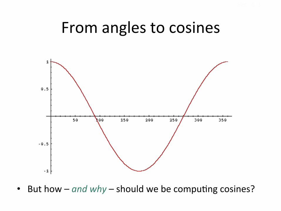
Fromanglestocosines
• Buthow–andwhy–shouldwebecompu1ngcosines?
Sec. 6.3
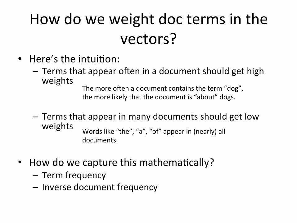
Howdoweweightdoctermsinthevectors?
• Here’stheintui1on:– Termsthatappearoueninadocumentshouldgethighweights
– Termsthatappearinmanydocumentsshouldgetlowweights
• Howdowecapturethismathema1cally?– Termfrequency– Inversedocumentfrequency
Themoreouenadocumentcontainstheterm“dog”,themorelikelythatthedocumentis“about”dogs.
Wordslike“the”,“a”,“of”appearin(nearly)alldocuments.

TFIDF
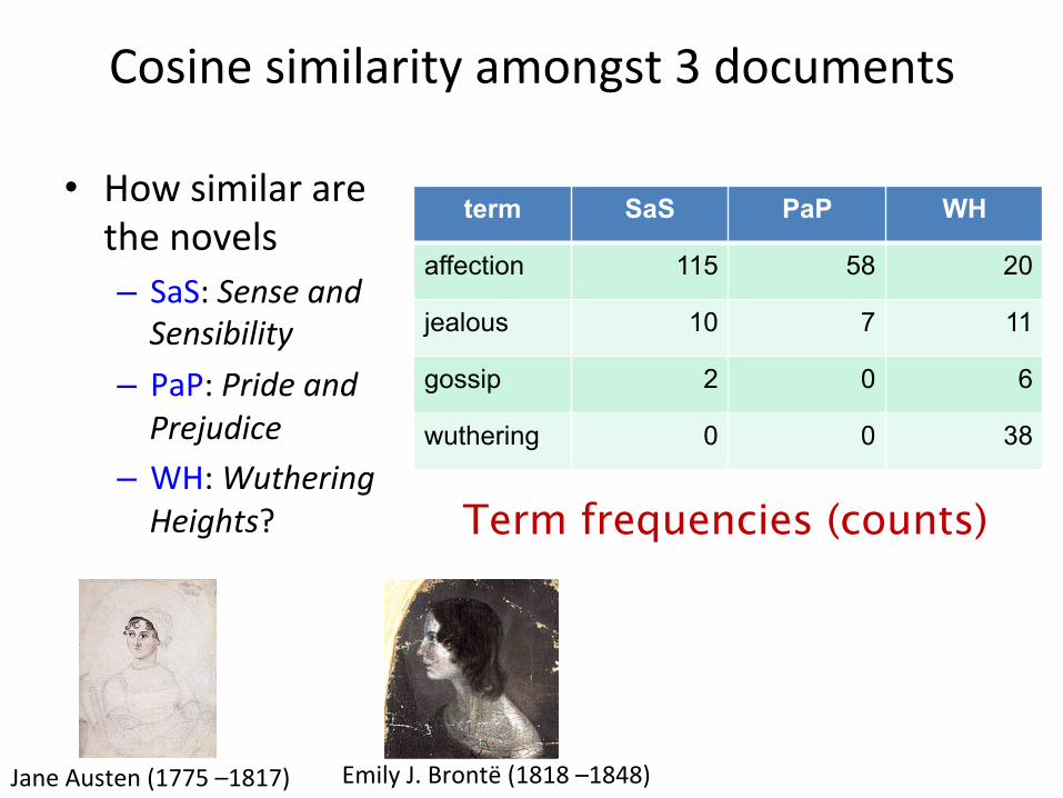
Cosinesimilarityamongst3documents
• Howsimilararethenovels– SaS:SenseandSensibility
– PaP:PrideandPrejudice
– WH:WutheringHeights?
term SaS PaP WH
affection 115 58 20
jealous 10 7 11
gossip 2 0 6
wuthering 0 0 38
Term frequencies (counts)
Sec. 6.3
JaneAusten(1775–1817) EmilyJ.Brontë(1818–1848)
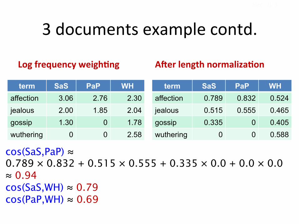
3documentsexamplecontd.
LogfrequencyweighMng
term SaS PaP WH affection 3.06 2.76 2.30 jealous 2.00 1.85 2.04 gossip 1.30 0 1.78 wuthering 0 0 2.58
ANerlengthnormalizaMon
term SaS PaP WH affection 0.789 0.832 0.524 jealous 0.515 0.555 0.465 gossip 0.335 0 0.405 wuthering 0 0 0.588
cos(SaS,PaP) ≈ 0.789 × 0.832 + 0.515 × 0.555 + 0.335 × 0.0 + 0.0 × 0.0 ≈ 0.94 cos(SaS,WH) ≈ 0.79 cos(PaP,WH) ≈ 0.69
Sec. 6.3
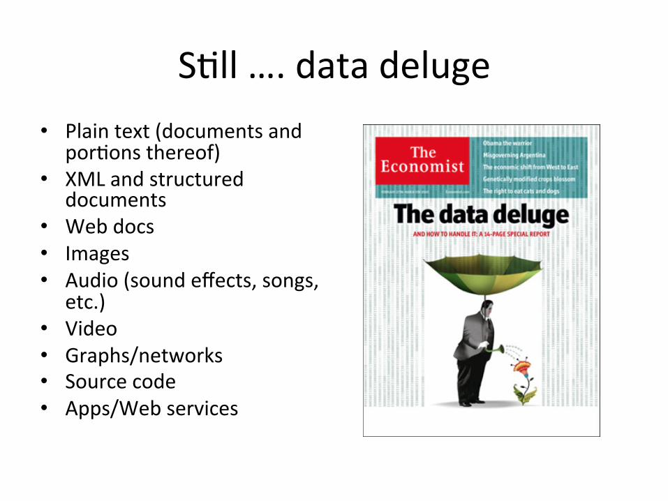
S1ll….datadeluge• Plaintext(documentsand
por1onsthereof)• XMLandstructured
documents• Webdocs• Images• Audio(soundeffects,songs,
etc.)• Video• Graphs/networks• Sourcecode• Apps/Webservices
Knowledge Discovery in Databases
“The non-trivial process of identifying valid, novel, potentially useful and ultimately understandable patterns in data”
Fayyad, Piatetsky-Shapiro, Smith [1996]
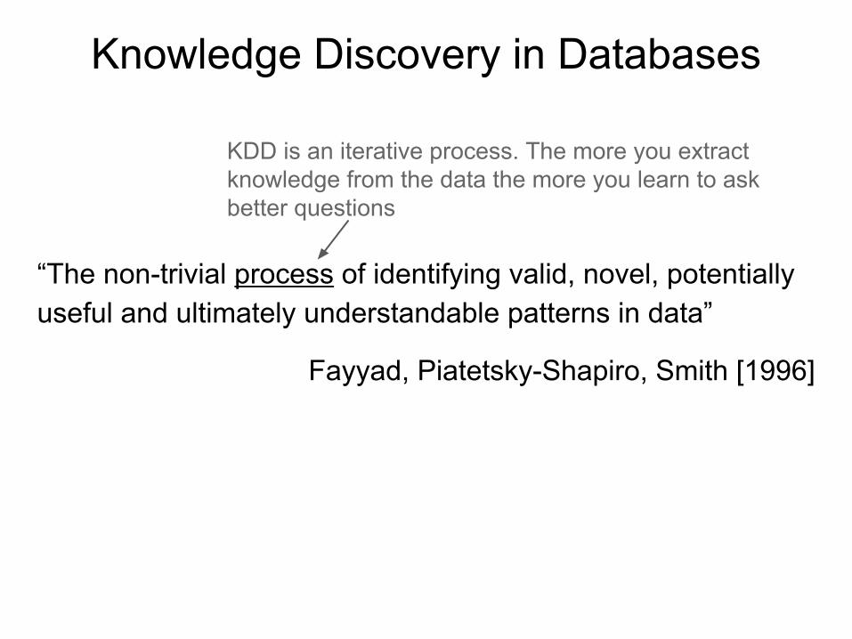
Knowledge Discovery in Databases
“The non-trivial process of identifying valid, novel, potentially useful and ultimately understandable patterns in data”
Fayyad, Piatetsky-Shapiro, Smith [1996]
KDD is an iterative process. The more you extract knowledge from the data the more you learn to ask better questions
Not something we already know
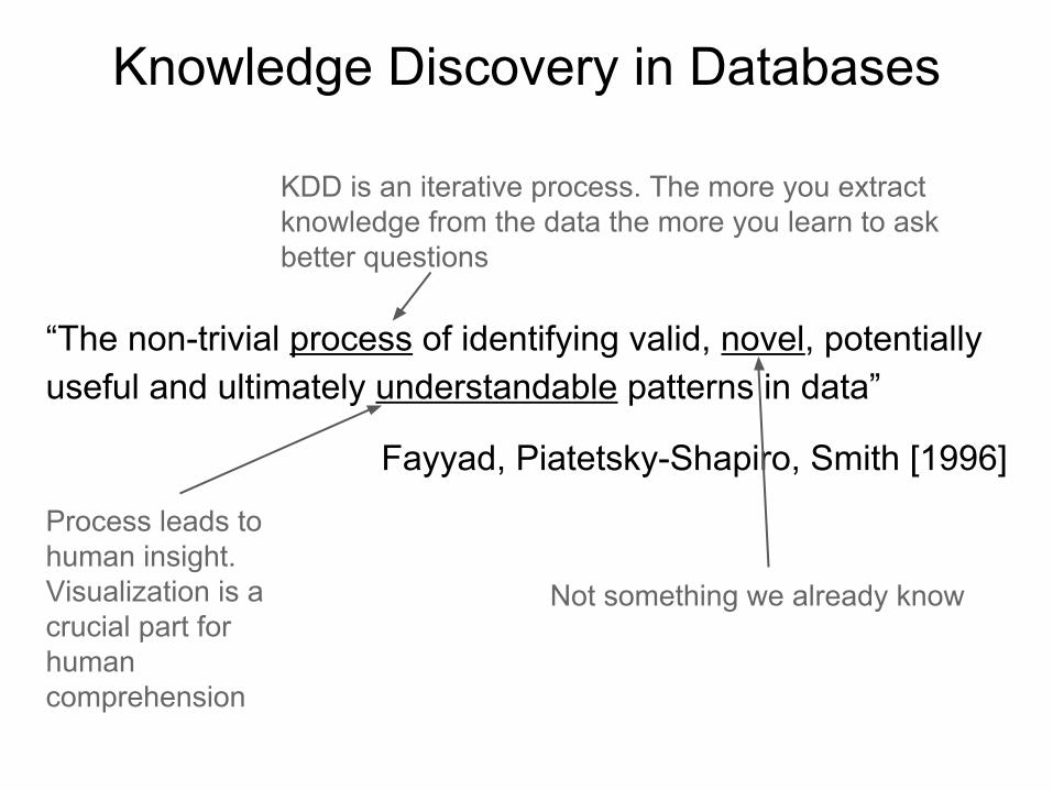
Process leads to human insight. Visualization is a crucial part for human comprehension

Knowledge Discovery in Databases
“The non-trivial process of identifying valid, novel, potentially useful and ultimately understandable patterns in data”
Fayyad, Piatetsky-Shapiro, Smith [1996]
KDD is an iterative process. The more you extract knowledge from the data the more you learn to ask better questions
Not something we already know
Process leads to human insight. Visualization is a crucial part for human comprehension Can generalize the
future
Machine Learning
Machine Learning at its most basic is the practice of using algorithms to parse data, learn from it, and then make a determination or prediction about something in the world
Usually, machine learning is focused on making prediction from examples (supervised learning) while KDD or Data Mining is focused on finding patterns (unsupervised learning).
Historically developed for different contexts (AI vs. Data Analytics), in practice based on the same ideas and techniques
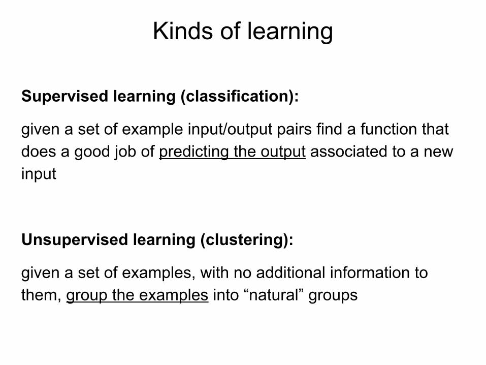
Kinds of learning
Supervised learning (classification):
given a set of example input/output pairs find a function that does a good job of predicting the output associated to a new input
Unsupervised learning (clustering):
given a set of examples, with no additional information to them, group the examples into “natural” groups
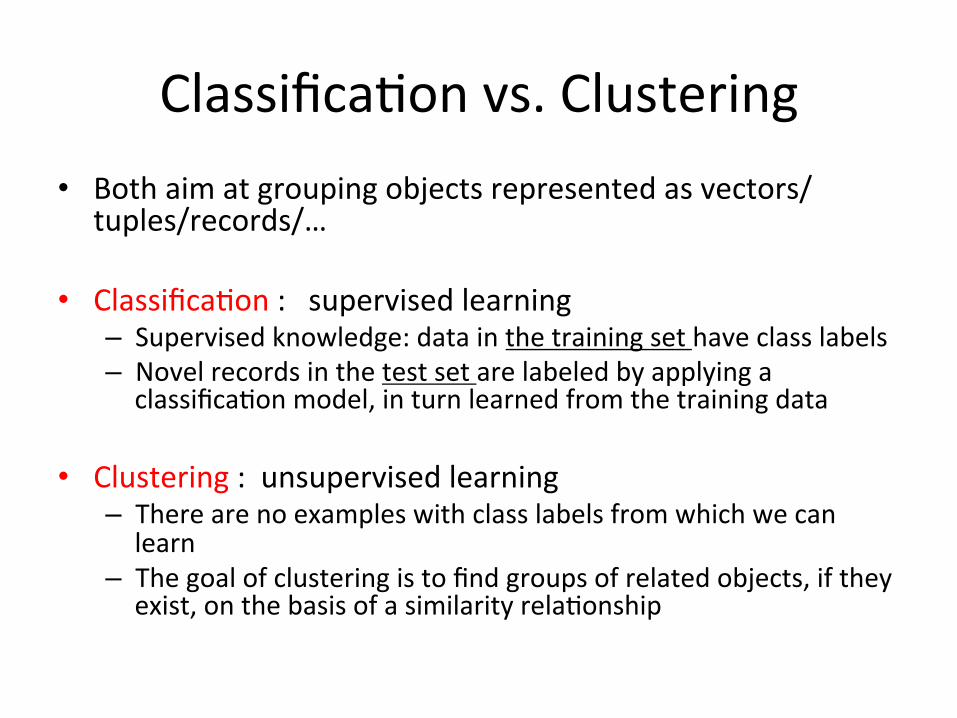
Classifica1onvs.Clustering• Bothaimatgroupingobjectsrepresentedasvectors/
tuples/records/…
• Classifica1on:supervisedlearning– Supervisedknowledge:datainthetrainingsethaveclasslabels– Novelrecordsinthetestsetarelabeledbyapplyingaclassifica1onmodel,inturnlearnedfromthetrainingdata
• Clustering:unsupervisedlearning– Therearenoexampleswithclasslabelsfromwhichwecanlearn
– Thegoalofclusteringistofindgroupsofrelatedobjects,iftheyexist,onthebasisofasimilarityrela1onship
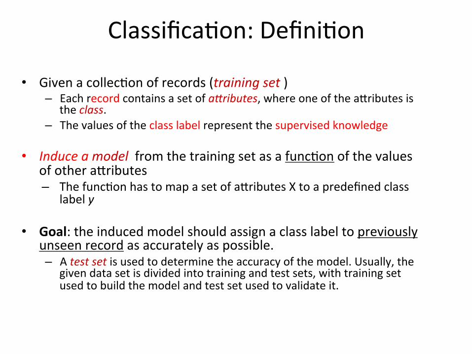
Classifica1on:Defini1on
• Givenacollec1onofrecords(trainingset)– EachrecordcontainsasetofaGributes,whereoneofthea+ributesis
theclass.– Thevaluesoftheclasslabelrepresentthesupervisedknowledge
• Induceamodelfromthetrainingsetasafunc1onofthevaluesofothera+ributes– Thefunc1onhastomapasetofa+ributesXtoapredefinedclass
labely
• Goal:theinducedmodelshouldassignaclasslabeltopreviouslyunseenrecordasaccuratelyaspossible.– Atestsetisusedtodeterminetheaccuracyofthemodel.Usually,the
givendatasetisdividedintotrainingandtestsets,withtrainingsetusedtobuildthemodelandtestsetusedtovalidateit.

Binary classifiers
The simplest form of classifiers are the binary classifiers:
Only two output classes: “yes” or “no”
A multi-class classifier can be created from a set of binary classifiers predicting the inclusion of each record to one of the multiple classes.
Input record Binary Classifier
Yes
No

Illustra1ngClassifica1onTask
Apply Model
Induction
Deduction
Learn Model
Model
Tid Attrib1 Attrib2 Attrib3 Class
1 Yes Large 125K No
2 No Medium 100K No
3 No Small 70K No
4 Yes Medium 120K No
5 No Large 95K Yes
6 No Medium 60K No
7 Yes Large 220K No
8 No Small 85K Yes
9 No Medium 75K No
10 No Small 90K Yes 10
Tid Attrib1 Attrib2 Attrib3 Class
11 No Small 55K ?
12 Yes Medium 80K ?
13 Yes Large 110K ?
14 No Small 95K ?
15 No Large 67K ? 10
Test Set
Learningalgorithm
Training Set
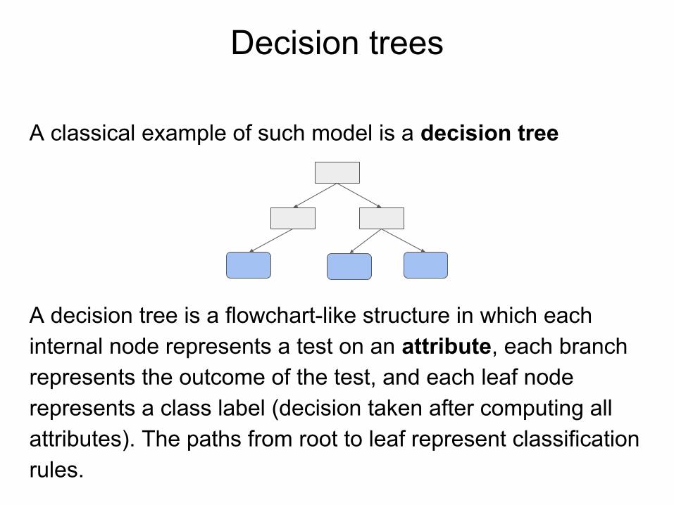
Decision trees
A classical example of such model is a decision tree
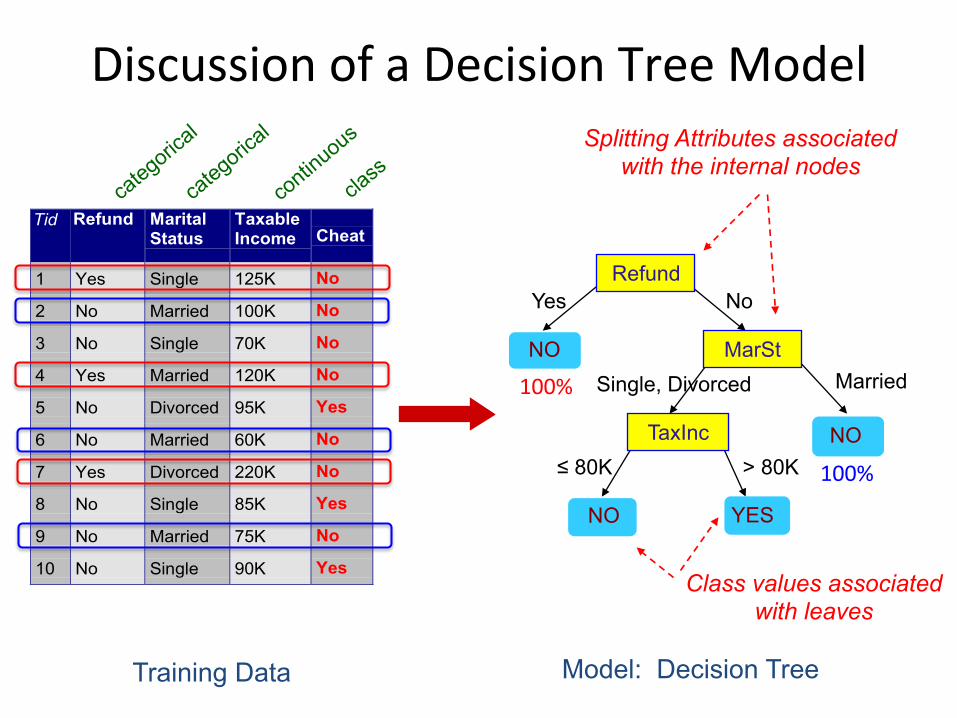
A decision tree is a flowchart-like structure in which each internal node represents a test on an attribute, each branch represents the outcome of the test, and each leaf node represents a class label (decision taken after computing all attributes). The paths from root to leaf represent classification rules.
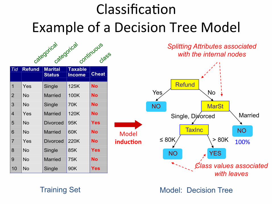
Classifica1onExampleofaDecisionTreeModel
Tid Refund MaritalStatus
TaxableIncome Cheat
1 Yes Single 125K No
2 No Married 100K No
3 No Single 70K No
4 Yes Married 120K No
5 No Divorced 95K Yes
6 No Married 60K No
7 Yes Divorced 220K No
8 No Single 85K Yes
9 No Married 75K No
10 No Single 90K Yes10
Refund
MarSt
TaxInc
YES NO
NO
NO
Yes No
Married Single, Divorced
≤ 80K > 80K
Splitting Attributes associated with the internal nodes
Training Set Model: Decision Tree
Class values associated with leaves
100%Model
inducMon

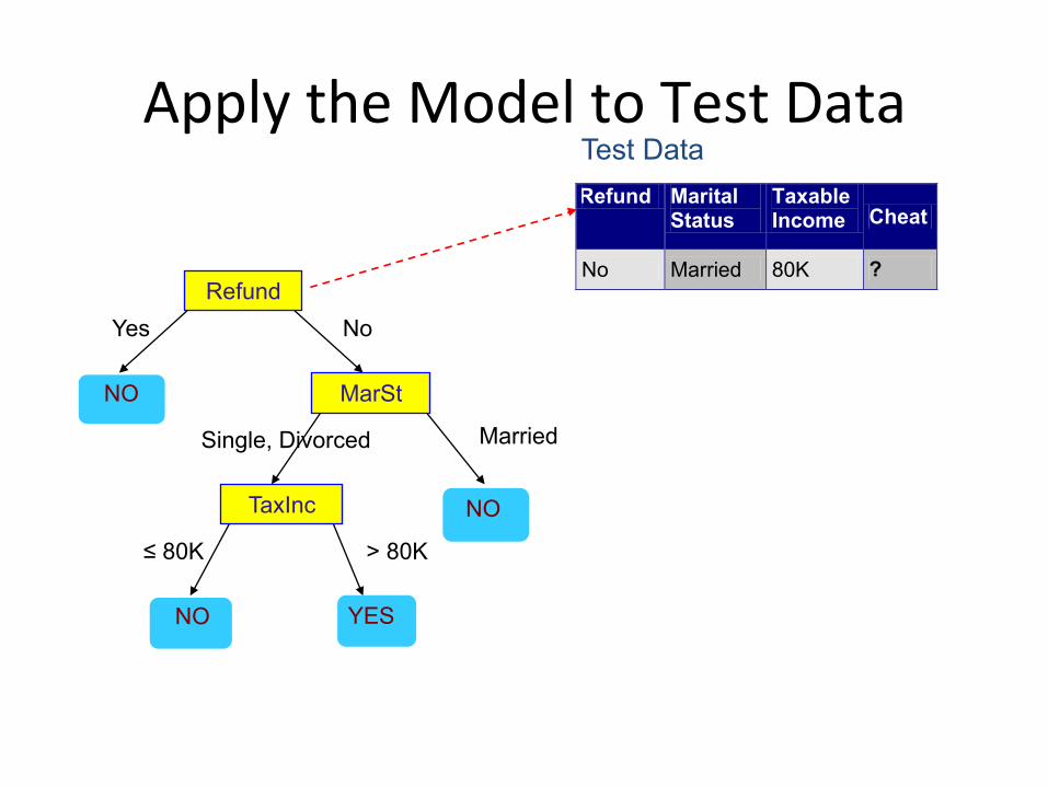
ApplytheModeltoTestData
Refund
MarSt
TaxInc
YES NO
NO
NO
Yes No
Married Single, Divorced
≤ 80K > 80K
Refund Marital Status
Taxable Income Cheat
No Married 80K ? 10
Test Data Start from the root of tree.
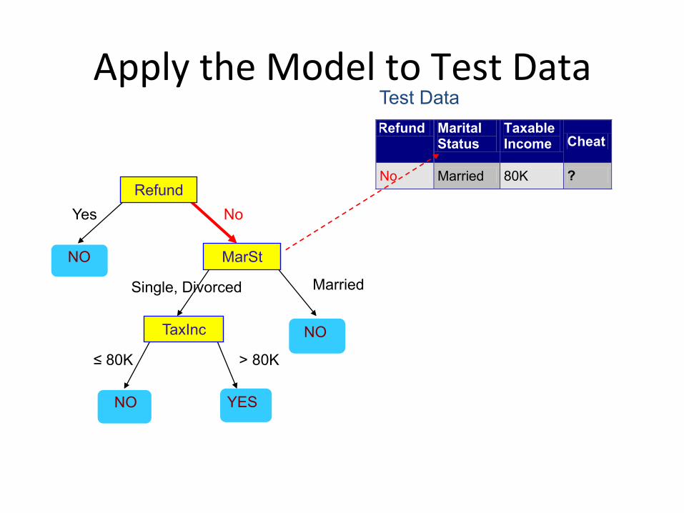
ApplytheModeltoTestData
Refund
MarSt
TaxInc
YES NO
NO
NO
Yes No
Married Single, Divorced
≤ 80K > 80K
Refund Marital Status
Taxable Income Cheat
No Married 80K ? 10
Test Data

ApplytheModeltoTestData
Refund
MarSt
TaxInc
YES NO
NO
NO
Yes No
Married Single, Divorced
≤ 80K > 80K
Refund Marital Status
Taxable Income Cheat
No Married 80K ? 10
Test Data
ApplytheModeltoTestData
Refund
MarSt
TaxInc
YES NO
NO
NO
Yes No
Married Single, Divorced
≤ 80K > 80K
Refund Marital Status
Taxable Income Cheat
No Married 80K ? 10
Test Data
ApplytheModeltoTestData
Refund
MarSt
TaxInc
YES NO
NO
NO
Yes No
Married Single, Divorced
≤ 80K > 80K
Refund Marital Status
Taxable Income Cheat
No Married 80K ? 10
Test Data

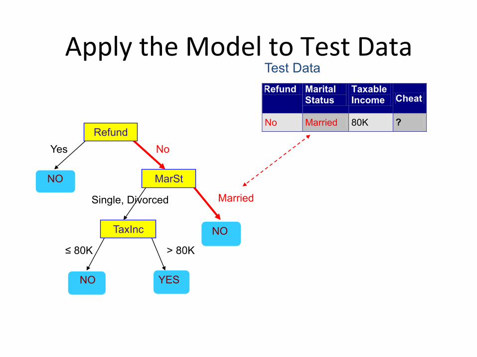
ApplytheModeltoTestData
Refund
MarSt
TaxInc
YES NO
NO
NO
Yes No
Married Single, Divorced
≤ 80K > 80K
Refund Marital Status
Taxable Income Cheat
No Married 80K ? 10
Test Data
Assign Cheat to �No�

DiscussionofaDecisionTreeModel
Tid Refund MaritalStatus
TaxableIncome Cheat
1 Yes Single 125K No
2 No Married 100K No
3 No Single 70K No
4 Yes Married 120K No
5 No Divorced 95K Yes
6 No Married 60K No
7 Yes Divorced 220K No
8 No Single 85K Yes
9 No Married 75K No
10 No Single 90K Yes10
Refund
MarSt
TaxInc
YES NO
NO
NO
Yes No
Married Single, Divorced
≤ 80K > 80K
Splitting Attributes associated with the internal nodes
Training Data Model: Decision Tree
Class values associated with leaves
100%
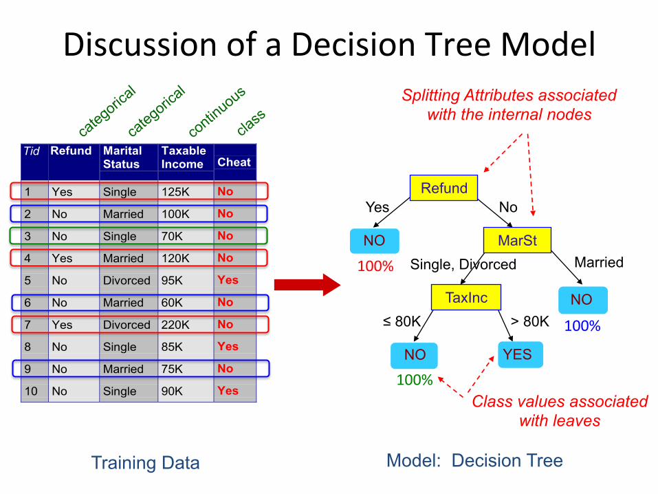
100%
100%

DiscussionofaDecisionTreeModel
Tid Refund MaritalStatus
TaxableIncome Cheat
1 Yes Single 125K No
2 No Married 100K No
3 No Single 70K No
4 Yes Married 120K No
5 No Divorced 95K Yes
6 No Married 60K No
7 Yes Divorced 220K No
8 No Single 85K Yes
9 No Married 75K No
10 No Single 90K Yes10
Refund
MarSt
TaxInc
YES NO
NO
NO
Yes No
Married Single, Divorced
≤ 80K > 80K
Splitting Attributes associated with the internal nodes
Training Data Model: Decision Tree
Class values associated with leaves
100%
100%
100% 100%
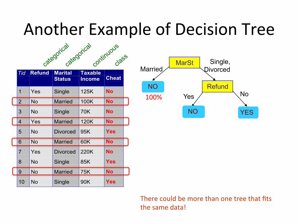
AnotherExampleofDecisionTree
Tid Refund MaritalStatus
TaxableIncome Cheat
1 Yes Single 125K No
2 No Married 100K No
3 No Single 70K No
4 Yes Married 120K No
5 No Divorced 95K Yes
6 No Married 60K No
7 Yes Divorced 220K No
8 No Single 85K Yes
9 No Married 75K No
10 No Single 90K Yes10
MarSt
Refund
YES
NO
NO
Yes No
Married Single,
Divorced
Therecouldbemorethanonetreethatfitsthesamedata!
100%
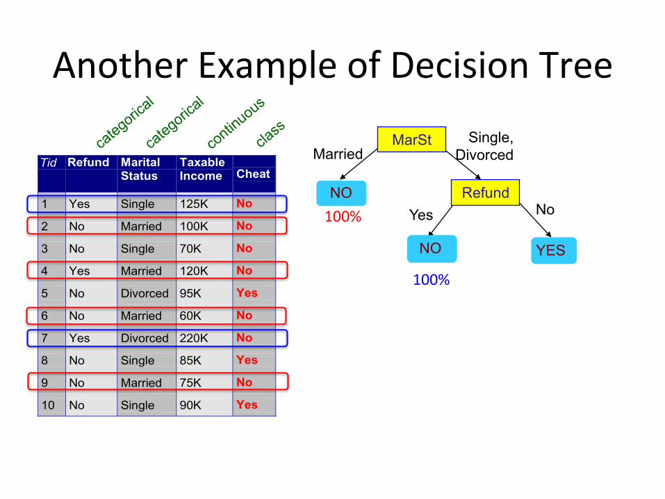
AnotherExampleofDecisionTree
Tid Refund MaritalStatus
TaxableIncome Cheat
1 Yes Single 125K No
2 No Married 100K No
3 No Single 70K No
4 Yes Married 120K No
5 No Divorced 95K Yes
6 No Married 60K No
7 Yes Divorced 220K No
8 No Single 85K Yes
9 No Married 75K No
10 No Single 90K Yes10
MarSt
Refund
YES
NO
NO
Yes No
Married Single,
Divorced
100%
100%
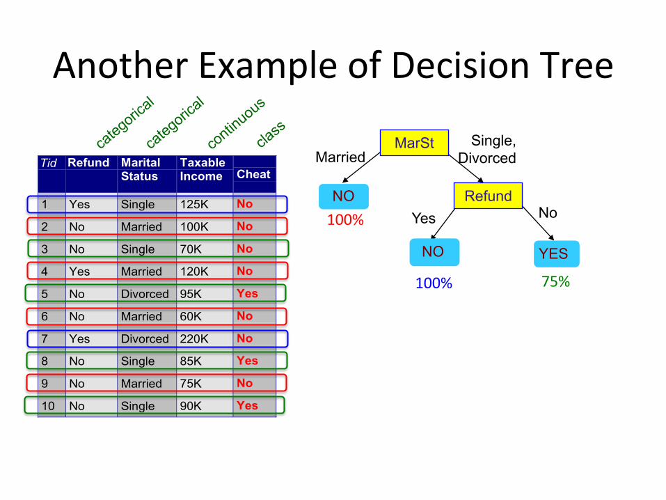
AnotherExampleofDecisionTree
Tid Refund MaritalStatus
TaxableIncome Cheat
1 Yes Single 125K No
2 No Married 100K No
3 No Single 70K No
4 Yes Married 120K No
5 No Divorced 95K Yes
6 No Married 60K No
7 Yes Divorced 220K No
8 No Single 85K Yes
9 No Married 75K No
10 No Single 90K Yes10
MarSt
Refund
YES
NO
NO
Yes No
Married Single,
Divorced
100%
100% 75%
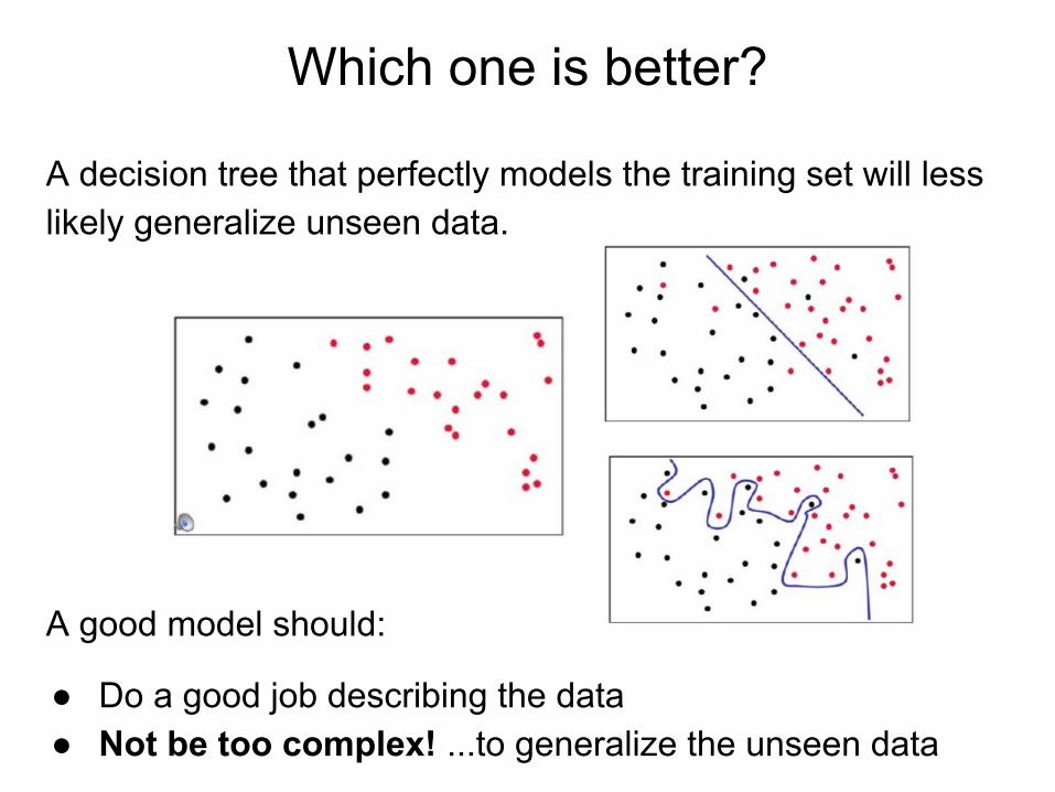
Which one is better?
A decision tree that perfectly models the training set will less likely generalize unseen data.
A good model should:
● Do a good job describing the data● Not be too complex! ...to generalize the unseen data
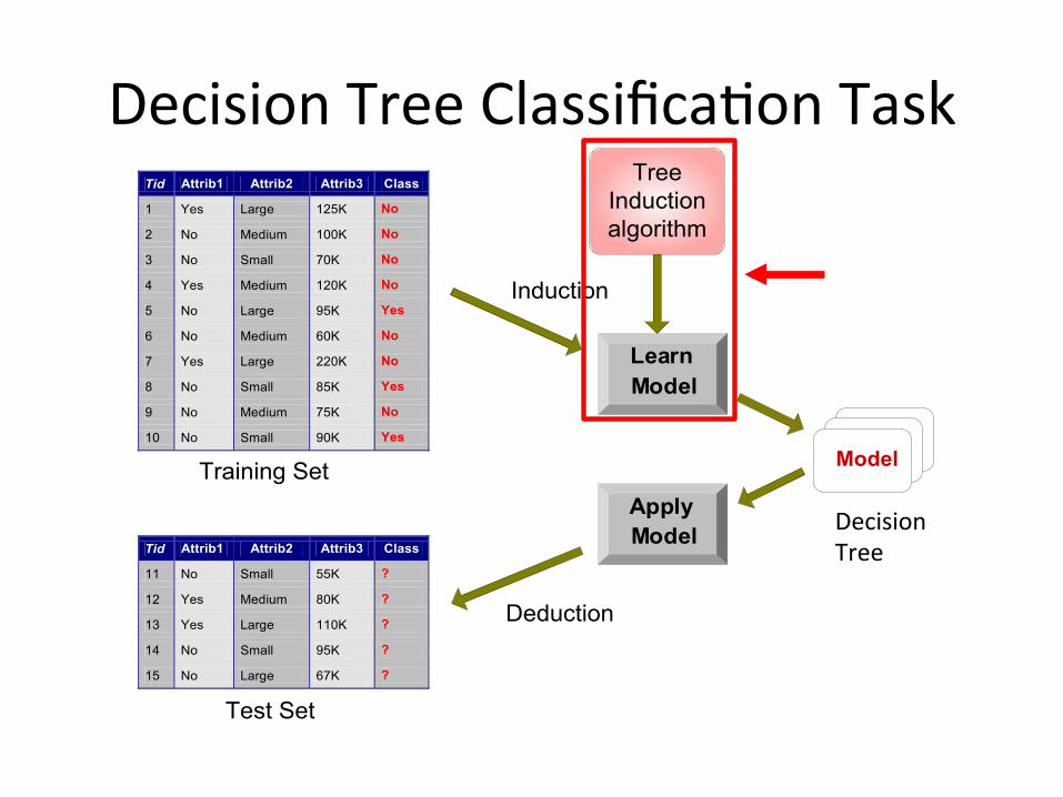
DecisionTreeClassifica1onTask
Apply Model
Induction
Deduction
Learn Model
Model
Tid Attrib1 Attrib2 Attrib3 Class
1 Yes Large 125K No
2 No Medium 100K No
3 No Small 70K No
4 Yes Medium 120K No
5 No Large 95K Yes
6 No Medium 60K No
7 Yes Large 220K No
8 No Small 85K Yes
9 No Medium 75K No
10 No Small 90K Yes 10
Tid Attrib1 Attrib2 Attrib3 Class
11 No Small 55K ?
12 Yes Medium 80K ?
13 Yes Large 110K ?
14 No Small 95K ?
15 No Large 67K ? 10
Test Set
TreeInductionalgorithm
Training Set
DecisionTree
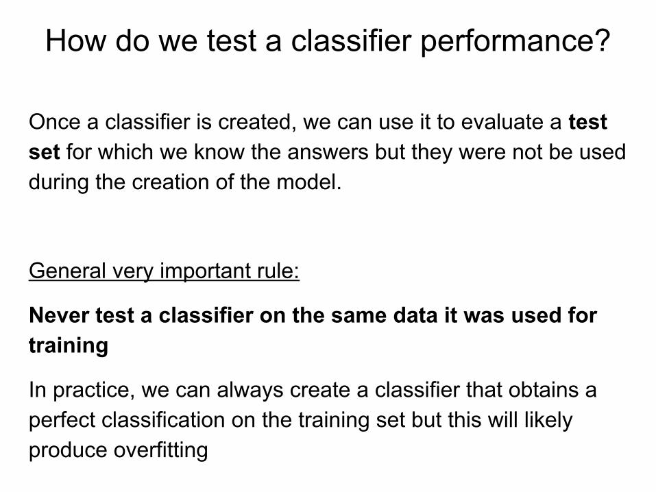
How do we test a classifier performance?
Once a classifier is created, we can use it to evaluate a test set for which we know the answers but they were not be used during the creation of the model.
General very important rule:
Never test a classifier on the same data it was used for training
In practice, we can always create a classifier that obtains a perfect classification on the training set but this will likely produce overfitting
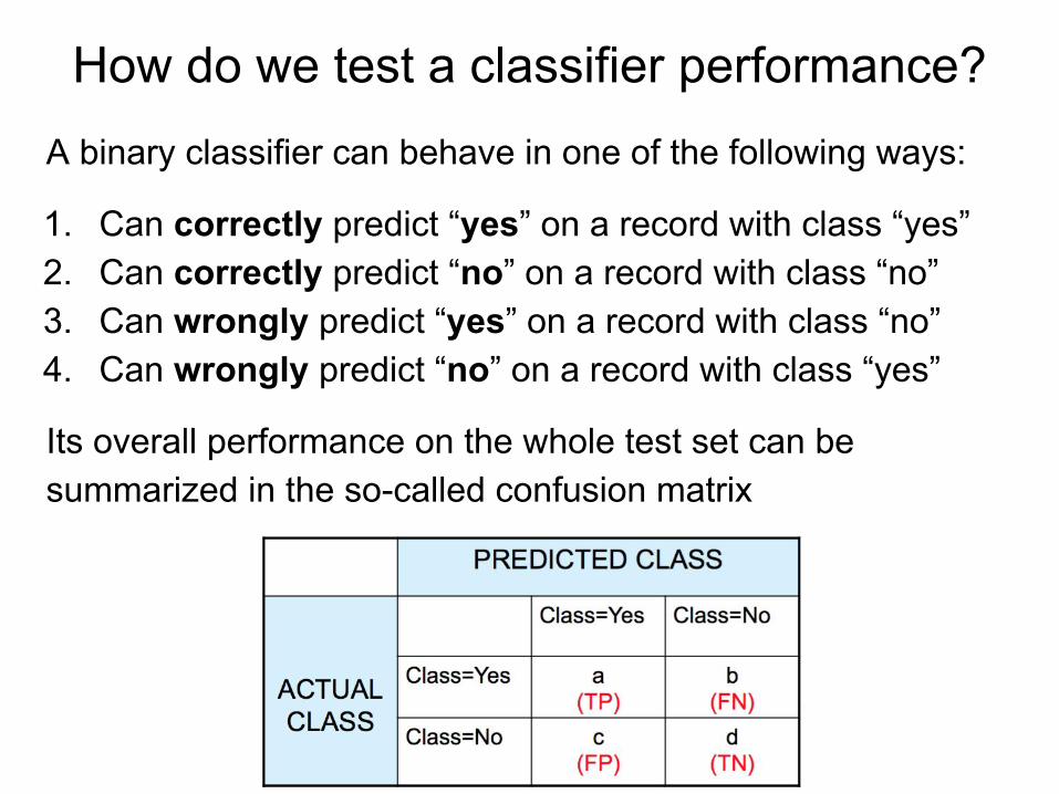
How do we test a classifier performance?A binary classifier can behave in one of the following ways:
1. Can correctly predict “yes” on a record with class “yes”2. Can correctly predict “no” on a record with class “no”3. Can wrongly predict “yes” on a record with class “no”4. Can wrongly predict “no” on a record with class “yes”
Its overall performance on the whole test set can be summarized in the so-called confusion matrix

How do we test a classifier performance?
Depending on the application, more or less importance can be given to answer correctly to “yes” and “no” classes.
Precision = TP / (TP+FP)
High precision means that every item labeled as “positive” does indeed belong to class “positive” (but says nothing about the number of items from class “positive” that were not labeled correctly).
What is the precision of a classifier that correctly answers “yes” just once? Is it useful?
How do we test a classifier performance?
Depending on the application, more or less importance can be given to answer correctly to “yes” and “no” classes.
Specificity = TN / (TN+FP)
measures the proportion of negatives that are correctly identified as such.
Similar to precision, but focusing the negative cases...

How do we test a classifier performance?
Depending on the application, more or less importance can be given to answer correctly to “yes” and “no” classes.
Sensitivity (or recall) = TP / (TP+FN)
High sensitivity means that every item from class positive was labeled as “yes” (but says nothing about how many other items were incorrectly also labeled “yes”).
What is the sensitivity of a classifier that always answers “yes”? But, in this case, what happens to the precision?
Some examples
We are developing a classifier that detects fraud in bank transactions.
Should we favor sensitivity (the ability to find most of the frauds) or precision (being absolutely sure that a detected fraud was indeed a fraud)?
Some examples
We are developing a classifier that detects fraud in bank transactions.
Should we favor sensitivity (the ability to find most of the frauds) or precision (being absolutely sure that a detected fraud was indeed a fraud)?
...it is desirable that we have a very high sensitivity, ie. most of the fraudulent transactions are identified, probably at loss of precision, since it is very important that all fraud is identified or at least suspicions are raised
Some examples
The zombie apocalypse is in progress, we want a classifier that accepts or rejects people in our safe zone.
Should we favor sensitivity (the ability to identify most of the healthy people) or precision (we should be absolutely sure that only healthy people should pass)?
Some examples
The zombie apocalypse is in progress, we want a classifier that accepts or rejects people in our safe zone.
Should we favor sensitivity (the ability to identify most of the healthy people) or precision (we should be absolutely sure that only healthy people should pass)?
Since one single mistakenly zombie in our safe zone will result in a disaster, we should favor precision over the ability to accept as many healthy people as possible...
Clustering
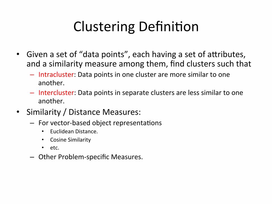
ClusteringDefini1on
• Givenasetof“datapoints”,eachhavingasetofa+ributes,andasimilaritymeasureamongthem,findclusterssuchthat– Intracluster:Datapointsinoneclusteraremoresimilartoone
another.– Intercluster:Datapointsinseparateclustersarelesssimilartoone
another.• Similarity/DistanceMeasures:
– Forvector-basedobjectrepresenta1ons• EuclideanDistance.• CosineSimilarity• etc.
– OtherProblem-specificMeasures.

WhatisClusterAnalysis?
• Findinggroupsofobjectssuchthattheobjectsinagroupwillbesimilar(orrelated)tooneanotheranddifferentfrom(orunrelatedto)theobjectsinothergroups
Inter-cluster distances are maximized
Intra-cluster distances are
minimized
Eachpointisavector<x,y,z>
Forexample,eachofx,y,zisthefrequencyofadis1nct
terminadocument
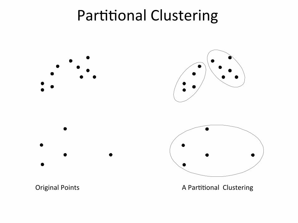
Par11onalClustering
OriginalPoints APar11onalClustering
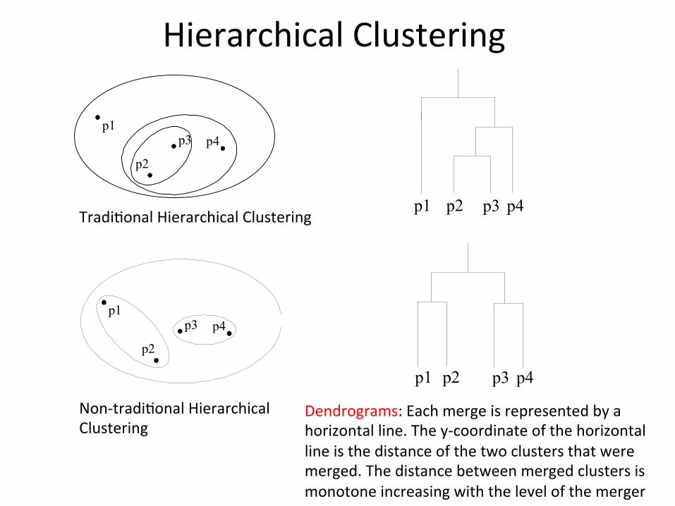
HierarchicalClustering
p4p1
p3
p2
p4 p1
p3
p2
p4p1 p2 p3
p4p1 p2 p3
Tradi1onalHierarchicalClustering
Non-tradi1onalHierarchicalClustering
Dendrograms:Eachmergeisrepresentedbyahorizontalline.They-coordinateofthehorizontallineisthedistanceofthetwoclustersthatweremerged.Thedistancebetweenmergedclustersismonotoneincreasingwiththelevelofthemerger
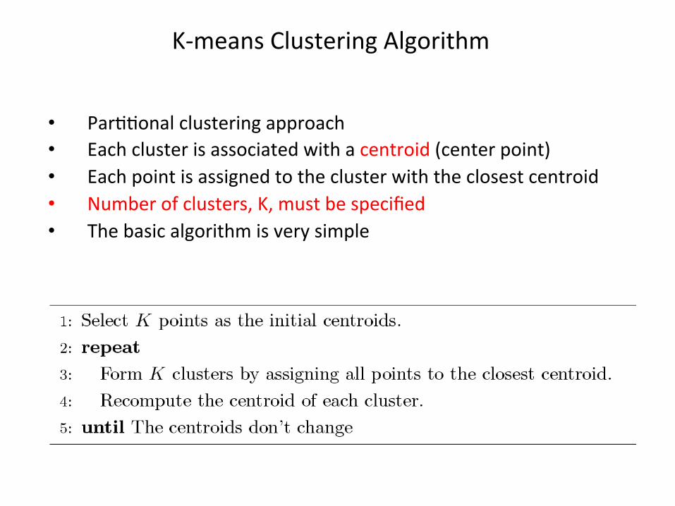
K-meansClusteringAlgorithm
• Par11onalclusteringapproach• Eachclusterisassociatedwithacentroid(centerpoint)• Eachpointisassignedtotheclusterwiththeclosestcentroid• Numberofclusters,K,mustbespecified• Thebasicalgorithmisverysimple

K-means interactive demo
http://stanford.edu/class/ee103/visualizations/kmeans/kmeans.html
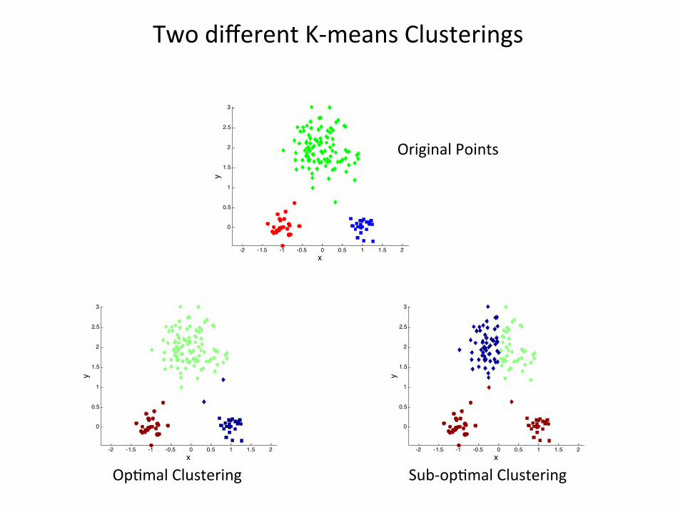
TwodifferentK-meansClusteringsTwodifferentK-meansClusterings
-2 -1.5 -1 -0.5 0 0.5 1 1.5 2
0
0.5
1
1.5
2
2.5
3
x
y
-2 -1.5 -1 -0.5 0 0.5 1 1.5 2
0
0.5
1
1.5
2
2.5
3
x
y
Sub-op1malClustering
-2 -1.5 -1 -0.5 0 0.5 1 1.5 2
0
0.5
1
1.5
2
2.5
3
x
y
Op1malClustering
OriginalPoints
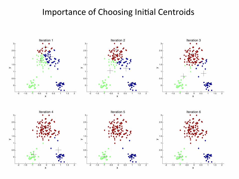
ImportanceofChoosingIni1alCentroidsImportanceofChoosingIni1alCentroids
-2 -1.5 -1 -0.5 0 0.5 1 1.5 2
0
0.5
1
1.5
2
2.5
3
x
y
Iteration 1
-2 -1.5 -1 -0.5 0 0.5 1 1.5 2
0
0.5
1
1.5
2
2.5
3
x
y
Iteration 2
-2 -1.5 -1 -0.5 0 0.5 1 1.5 2
0
0.5
1
1.5
2
2.5
3
x
y
Iteration 3
-2 -1.5 -1 -0.5 0 0.5 1 1.5 2
0
0.5
1
1.5
2
2.5
3
x
y
Iteration 4
-2 -1.5 -1 -0.5 0 0.5 1 1.5 2
0
0.5
1
1.5
2
2.5
3
x
y
Iteration 5
-2 -1.5 -1 -0.5 0 0.5 1 1.5 2
0
0.5
1
1.5
2
2.5
3
x
y
Iteration 6

ImportanceofChoosingIni1alCentroids…ImportanceofChoosingIni1alCentroids…
-2 -1.5 -1 -0.5 0 0.5 1 1.5 2
0
0.5
1
1.5
2
2.5
3
x
yIteration 1
-2 -1.5 -1 -0.5 0 0.5 1 1.5 2
0
0.5
1
1.5
2
2.5
3
x
y
Iteration 2
-2 -1.5 -1 -0.5 0 0.5 1 1.5 2
0
0.5
1
1.5
2
2.5
3
x
y
Iteration 3
-2 -1.5 -1 -0.5 0 0.5 1 1.5 2
0
0.5
1
1.5
2
2.5
3
x
y
Iteration 4
-2 -1.5 -1 -0.5 0 0.5 1 1.5 2
0
0.5
1
1.5
2
2.5
3
xy
Iteration 5
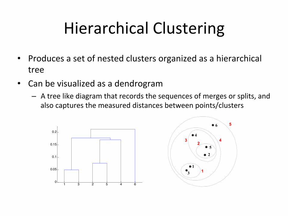
HierarchicalClustering• Producesasetofnestedclustersorganizedasahierarchical
tree• Canbevisualizedasadendrogram
– Atreelikediagramthatrecordsthesequencesofmergesorsplits,andalsocapturesthemeasureddistancesbetweenpoints/clusters
1 3 2 5 4 60
0.05
0.1
0.15
0.2
1
2
3
4
5
6
1
23 4
5

StrengthsofHierarchicalClustering• Donothavetoassumeanypar1cularnumberofclusters
– Anydesirednumberofclusterscanbeobtainedby�cuÑng�thedendogramattheproperlevel
• Theymaycorrespondtomeaningfultaxonomies
– Exampleinbiologicalsciences(e.g.,animalkingdom,phylogenyreconstruc1on,…)

HierarchicalClustering• Twomaintypesofhierarchicalclustering
– Agglomera1ve:• Startwiththepointsasindividualclusters• Ateachstep,mergetheclosestpairofclustersun1lonlyonecluster(orkclusters)leu
– Divisive:• Startwithone,all-inclusivecluster• Ateachstep,splitaclusterun1leachclustercontainsapoint(ortherearekclusters)
• Bisec1ngk-means
• Tradi1onalhierarchicalalgorithmsuseasimilarityordistancematrix– Mergeorsplitoneclusterata1me
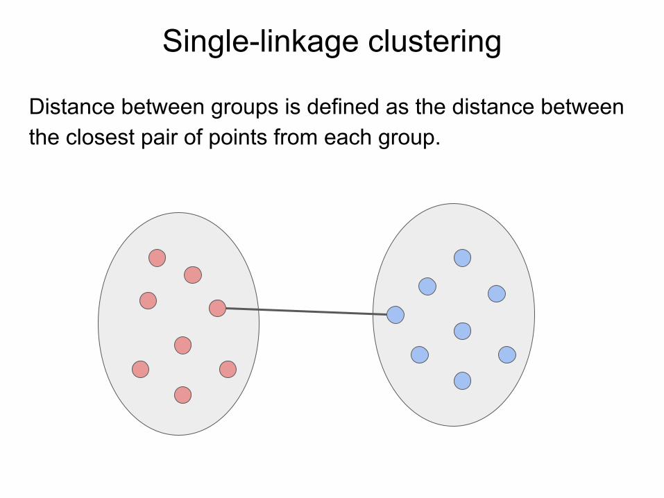
Single-linkage clustering
Distance between groups is defined as the distance between the closest pair of points from each group.
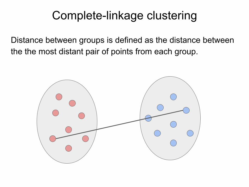
Complete-linkage clustering
Distance between groups is defined as the distance between the the most distant pair of points from each group.

Average-linkage clustering
The distance between two clusters is defined as the average of distances between all pairs of points (of opposite clusters)

Cutting the dendrogram
When we cut the dendrogram at a specific height we generate a set of clusters. The number of clusters can be specified a-posteriori by cutting the dendrogram
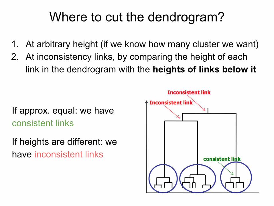
Where to cut the dendrogram?
1. At arbitrary height (if we know how many cluster we want)2. At inconsistency links, by comparing the height of each
link in the dendrogram with the heights of links below it
If approx. equal: we have consistent links
If heights are different: we have inconsistent links