Data Mining - Sharifce.sharif.edu/courses/94-95/1/ce714-1/resources/... · 244 Chapter 6 Mining Frequent Patterns, Associations, and Correlations ... co-occurring terms have numerous

Data MiningAssociative pattern mining

Hamid Beigy

Sharif University of Technology

Fall 1394

Hamid Beigy (Sharif University of Technology) Data Mining Fall 1394 1 / 64

Outline

1 Introduction

2 Frequent pattern mining model

3 Frequent itemset mining algorithmsBrute force Frequent itemset mining algorithmApriori algorithmFrequent pattern growth (FP-growth)Mining frequent itemsets using vertical data format

4 Summarizing itemsetsMining maximal itemsetsMining closed itemsets

5 Sequence mining

6 Graph mining

7 Pattern and rule assessment


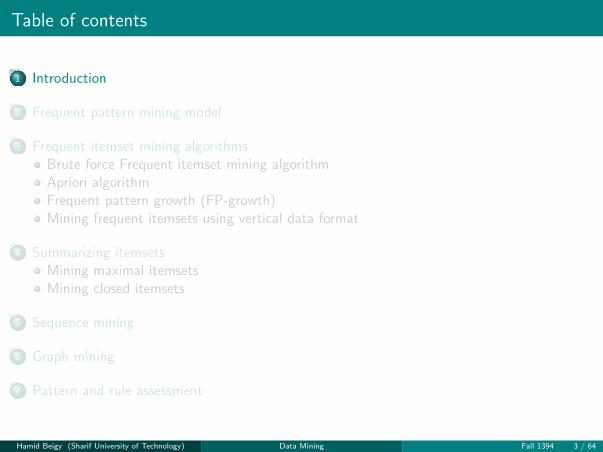
Table of contents

1 Introduction




5 Sequence mining

6 Graph mining



Introduction

The classical problem of associative pattern mining is defined in the context ofsupermarket (items bought by customers).

The items bought by customers are referred to as transactions.

The goal is to determine association between groups of items bought by customer.

The most popular model for associative pattern mining uses the frequencies of sets ofitems as the quantification of the level of association.

The discovered set of items are referred to as large itemsets, frequent itemsets, orfrequent patterns.

HAN 13-ch06-243-278-9780123814791 2011/6/1 3:20 Page 244 #2

244 Chapter 6 Mining Frequent Patterns, Associations, and Correlations

interesting associations and correlations between itemsets in transactional and relationaldatabases. We begin in Section 6.1.1 by presenting an example of market basket analysis,the earliest form of frequent pattern mining for association rules. The basic concepts ofmining frequent patterns and associations are given in Section 6.1.2.

6.1.1 Market Basket Analysis: A Motivating Example

Frequent itemset mining leads to the discovery of associations and correlations amongitems in large transactional or relational data sets. With massive amounts of data contin-uously being collected and stored, many industries are becoming interested in miningsuch patterns from their databases. The discovery of interesting correlation relation-ships among huge amounts of business transaction records can help in many busi-ness decision-making processes such as catalog design, cross-marketing, and customershopping behavior analysis.

A typical example of frequent itemset mining is market basket analysis. This processanalyzes customer buying habits by finding associations between the different items thatcustomers place in their “shopping baskets” (Figure 6.1). The discovery of these associa-tions can help retailers develop marketing strategies by gaining insight into which itemsare frequently purchased together by customers. For instance, if customers are buyingmilk, how likely are they to also buy bread (and what kind of bread) on the same trip

Which items are frequentlypurchased together by customers?

milkcerealbread milk bread

buttermilk breadsugar eggs

Customer 1

Market Analyst

Customer 2

sugareggs

Customer n

Customer 3

Shopping Baskets

Figure 6.1 Market basket analysis.Hamid Beigy (Sharif University of Technology) Data Mining Fall 1394 3 / 64

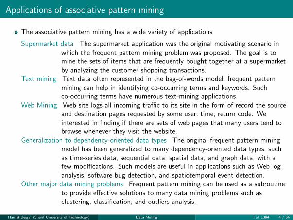
Applications of associative pattern mining

The associative pattern mining has a wide variety of applications

Supermarket data The supermarket application was the original motivating scenario inwhich the frequent pattern mining problem was proposed. The goal is tomine the sets of items that are frequently bought together at a supermarketby analyzing the customer shopping transactions.

Text mining Text data often represented in the bag-of-words model, frequent patternmining can help in identifying co-occurring terms and keywords. Suchco-occurring terms have numerous text-mining applications

Web Mining Web site logs all incoming traffic to its site in the form of record the sourceand destination pages requested by some user, time, return code. Weinterested in finding if there are sets of web pages that many users tend tobrowse whenever they visit the website.

Generalization to dependency-oriented data types The original frequent pattern miningmodel has been generalized to many dependency-oriented data types, suchas time-series data, sequential data, spatial data, and graph data, with afew modifications. Such models are useful in applications such as Web loganalysis, software bug detection, and spatiotemporal event detection.

Other major data mining problems Frequent pattern mining can be used as a subroutineto provide effective solutions to many data mining problems such asclustering, classification, and outliers analysis.


Association rules

Frequent itemsets can be used to generate association rules of the form

X =⇒ Y

X and Y are set of items.

For example, if the supermarket owner discovers the following rule

{Eggs,Milk} =⇒ {Yogurt}

As a conclusion, she/he can promote Yogurt to customers who often buy Eggs and Milk.

The frequency-based model for associative pattern mining is very popular due to itssimplicity.

However, the raw frequency of a pattern is not same as the statistical significance ofunderlying correlations.

Therefor several models based on statistical significance are proposed , which are referredto as interesting patterns.


Table of contents

1 Introduction




5 Sequence mining

6 Graph mining



Frequent pattern mining model

Assume that the database T contains n transactions T1,T2, . . . ,Tn.

Each transaction has a unique identifier, referred to as transaction identifier or tid.

Each transaction Ti is drawn on the universe of items U.

4.2. THE FREQUENT PATTERN MINING MODEL 89

tid Set of Items Binary Representation

1 {Bread,Butter,Milk} 1100102 {Eggs, Milk, Y ogurt} 0001113 {Bread,Cheese,Eggs,Milk} 1011104 {Eggs, Milk, Y ogurt} 0001115 {Cheese, Milk, Y ogurt} 001011

Table 4.1: Example of a snapshot of a market basket data set

The support of an itemset I is denoted by sup(I). Clearly, items that are correlated willfrequently occur together in transactions. Such itemsets will have high support. Therefore,the frequent pattern mining problem is that of determining itemsets that have the requisitelevel of minimum support.

Definition 4.2.2 (Frequent Itemset Mining) Given a set of transactions T ={T1 . . . Tn}, where each transaction Ti is a subset of items from U , determine all item-sets I that occur as a subset of at least a pre-defined fraction minsup of the transactions inT .

The pre-defined fraction minsup is referred to as the minimum support. While the defaultconvention in this book is to assume that minsup refers to a fractional relative value, itis also sometimes specified as an absolute integer value in terms of the raw number oftransactions. This chapter will always assume the convention of a relative value, unlessspecified otherwise. Frequent patterns are also referred to as frequent itemsets, or largeitemsets. This book will use these terms interchangeably.

The unique identifier of a transaction is referred to as a transaction identifier, or tid forshort. The frequent itemset mining problem may also be stated more generally in set-wiseform.

Definition 4.2.3 (Frequent Itemset Mining: Set-wise Definition) Given a set ofsets T = {T1 . . . Tn}, where each element of the set Ti is drawn on the universe of elementsU , determine all sets I that occur as a subset of at least a pre-defined fraction minsup ofthe sets in T .

As discussed in Chapter 1, binary multidimensional data and set data are equivalent. Thisequivalence is because each multidimensional attribute can represent a set element (oritem). A value of 1 for a multidimensional attribute corresponds to inclusion in the set (ortransaction). Therefore, a transaction data set (or set of sets) can also be represented as amultidimensional binary database whose dimensionality is equal to the number of items.

Consider the transactions illustrated in Table 4.1. Each transaction is associated with aunique transaction identifier in the leftmost column, and contains a baskets of items thatwere bought together at the same time. The right column in Table 4.1 contains the binarymultidimensional representation of the corresponding basket. The attributes of this binaryrepresentation are arranged in the order {Bread, Butter, Cheese, Eggs,Milk, Y ogurt}. Inthis database of 5 transactions, the support of {Bread,Milk} is 2/5 = 0.4 because bothitems in this basket occur in 2 out of a total of 5 transactions. Similarly, the support of{Cheese, Y ogurt} is 0.2 because it appears in only the last transaction. Therefore, if theminimum support is set to 0.3, then the itemset {Bread,Milk} will be reported but notthe itemset {Cheese, Y ogurt}.

The number of frequent itemsets is generally very sensitive to the minimum supportlevel. Consider the case where a minimum support level of 0.3 is used. Each of the items

An itemset is a set of items. A k−itemset is an itemset that contains exactly k items.

The fraction of transactions in T = {T1,T2, . . . ,Tn} in which an itemset occures as asubset is known as support of itemset.

Definition (Support)

The support of an itemset I is defined as the fraction of the transactions in the databaseT = {T1,T2, . . . ,Tn} that contain I as a subset and denoted by sup(I ).

Items that are correlated will have high support.


Frequent pattern mining model (cont.)

The frequent pattern mining model is to determine itemsets with a minimum level ofsupport denoted by minsup.

Definition (Frequent itemset mining)

Given a set of transactions T = {T1,T2, . . . ,Tn}, where each transaction Ti is a subset ofitems from U, determine all itemsets I that occur as a subset of at least a predefined fractionminsup of the transactions in T .

Consider the following database

128 CHAPTER 5. ASSOCIATION PATTERN MINING: ADVANCED CONCEPTS

tid Set of Items

1 {Bread,Butter,Milk}2 {Eggs, Milk, Y ogurt}3 {Bread,Cheese,Eggs,Milk}4 {Eggs, Milk, Y ogurt}5 {Cheese, Milk, Y ogurt}

Table 5.1: Example of a Snapshot of a Market Basket Data Set ( Replicated from Table 4.1)

scheme that is designed to assure non-redundancy. Similarly, there are fewer constraineditemsets than unconstrained itemsets. However, the shrinkage of the discovered itemsetsis because of the constraints rather than a compression or summarization scheme. Thischapter will also discuss a number of useful applications of association pattern mining.

This chapter is organized as follows. The problem of pattern summarization is addressedin section 5.2. A discussion of querying methods for pattern mining is provided in section 5.3.Section 5.4 discusses numerous applications of frequent pattern mining. The conclusions arediscussed in section 5.5.

5.2 Pattern Summarization

Frequent itemset mining algorithms often discover a large number of patterns. The size ofthe output creates challenges for users to assimilate the results and make meaningful in-ferences. An important observation is that the vast majority of the generated patterns areoften redundant. This is because of the downward closure property, which ensures that allsubsets of a frequent itemset are also frequent. There are different kinds of compact repre-sentations in frequent pattern mining that retain different levels of knowledge about the trueset of frequent patterns and their support values. The most well-known representations arethose of maximal frequent itemsets, closed frequent itemsets, and other approximate repre-sentations. These representations vary in the degree of information loss in the summarizedrepresentation. Closed representations are fully lossless with respect to the support andmembership of itemsets. Maximal representations are lossy with respect to the support butlossless with respect to membership of itemsets. Approximate condensed representations arelossy with respect to both but often provide the best practical alternative in application-driven scenarios.

5.2.1 Maximal Patterns

The concept of maximal itemsets was discussed briefly in the previous chapter. For conve-nience, the definition of maximal itemsets is restated here:

Definition 5.2.1 (Maximal Frequent Itemset) A frequent itemset is maximal at agiven minimum support level minsup if it is frequent and no superset of it is frequent.

For example, consider the example of Table 5.1, which is replicated from the example ofTable 4.1 in the previous chapter. It is evident that the itemset {Eggs, Milk, Y ogurt} isfrequent at a minimum support level of 2 and is also maximal. The support of propersubsets of a maximal itemset is always equal to, or strictly larger than the latter becauseof the support-monotonicity property. For example, the support of {Eggs, Milk}, whichis a proper subset of the itemset {Eggs, Milk, Y ogurt}, is 3. Therefore, one strategy forsummarization is to mine only the maximal itemsets. The remaining itemsets are derivedas subsets of the maximal itemsets.

The universe of items U = {Bread ,Butter ,Cheese,Eggs,Milk ,Yogurt}.sup({Bread ,Milk} = 2

5 = 0.4.

sup({Cheese,Yogurt} = 15 = 0.2.

The number of frequent itemsets is generally very sensitive to the value of minsup.

Therefore, an appropriate choice of minsup is crucial for discovering a set of frequentpatterns with meaningful size.



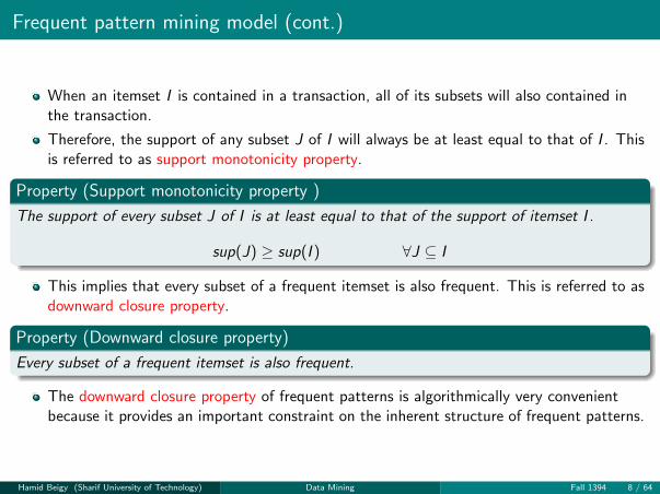
When an itemset I is contained in a transaction, all of its subsets will also contained inthe transaction.

Therefore, the support of any subset J of I will always be at least equal to that of I . Thisis referred to as support monotonicity property.

Property (Support monotonicity property )

The support of every subset J of I is at least equal to that of the support of itemset I .

sup(J) ≥ sup(I ) ∀J ⊆ I

This implies that every subset of a frequent itemset is also frequent. This is referred to asdownward closure property.

Property (Downward closure property)

Every subset of a frequent itemset is also frequent.

The downward closure property of frequent patterns is algorithmically very convenientbecause it provides an important constraint on the inherent structure of frequent patterns.



The downward closure property can be used to create concise representations of frequentpatterns, wherein only the maximal frequent subsets are retained.

Definition (Maximal frequent itemsets )

A frequent itemset is maximal at a given minimum support level minsup, if it is frequent, andno superset of it is frequent.


128 CHAPTER 5. ASSOCIATION PATTERN MINING: ADVANCED CONCEPTS

tid Set of Items

1 {Bread,Butter,Milk}2 {Eggs, Milk, Y ogurt}3 {Bread,Cheese,Eggs,Milk}4 {Eggs, Milk, Y ogurt}5 {Cheese, Milk, Y ogurt}

Table 5.1: Example of a Snapshot of a Market Basket Data Set ( Replicated from Table 4.1)

scheme that is designed to assure non-redundancy. Similarly, there are fewer constraineditemsets than unconstrained itemsets. However, the shrinkage of the discovered itemsetsis because of the constraints rather than a compression or summarization scheme. Thischapter will also discuss a number of useful applications of association pattern mining.

This chapter is organized as follows. The problem of pattern summarization is addressedin section 5.2. A discussion of querying methods for pattern mining is provided in section 5.3.Section 5.4 discusses numerous applications of frequent pattern mining. The conclusions arediscussed in section 5.5.

5.2 Pattern Summarization

Frequent itemset mining algorithms often discover a large number of patterns. The size ofthe output creates challenges for users to assimilate the results and make meaningful in-ferences. An important observation is that the vast majority of the generated patterns areoften redundant. This is because of the downward closure property, which ensures that allsubsets of a frequent itemset are also frequent. There are different kinds of compact repre-sentations in frequent pattern mining that retain different levels of knowledge about the trueset of frequent patterns and their support values. The most well-known representations arethose of maximal frequent itemsets, closed frequent itemsets, and other approximate repre-sentations. These representations vary in the degree of information loss in the summarizedrepresentation. Closed representations are fully lossless with respect to the support andmembership of itemsets. Maximal representations are lossy with respect to the support butlossless with respect to membership of itemsets. Approximate condensed representations arelossy with respect to both but often provide the best practical alternative in application-driven scenarios.

5.2.1 Maximal Patterns

The concept of maximal itemsets was discussed briefly in the previous chapter. For conve-nience, the definition of maximal itemsets is restated here:

Definition 5.2.1 (Maximal Frequent Itemset) A frequent itemset is maximal at agiven minimum support level minsup if it is frequent and no superset of it is frequent.

For example, consider the example of Table 5.1, which is replicated from the example ofTable 4.1 in the previous chapter. It is evident that the itemset {Eggs, Milk, Y ogurt} isfrequent at a minimum support level of 2 and is also maximal. The support of propersubsets of a maximal itemset is always equal to, or strictly larger than the latter becauseof the support-monotonicity property. For example, the support of {Eggs, Milk}, whichis a proper subset of the itemset {Eggs, Milk, Y ogurt}, is 3. Therefore, one strategy forsummarization is to mine only the maximal itemsets. The remaining itemsets are derivedas subsets of the maximal itemsets.

The itemset {Eggs,Milk ,Yogurt} is maximal frequent itemset at minsup = 0.3.

The itemset {Eggs,Milk} is not maximal, because it has a superset that is also frequent.

All frequent itemsets can be derived from the maximal patterns by enumerating thesubsets of the maximal frequent patterns.

The maximal patterns can be considered condensed representation of the frequentpatterns.



The maximal patterns can be considered condensed representation of frequent patterns.The condensed representation does not retain information about the support values of thesubsets. The support of {Eggs,Milk,Yogurt} is 0.4 and does not provide any informationabout the support of {Milk,Yogurt}, which is 0.6.A different representation called closed frequent itemset is able to retain supportinformation of the subsets. (will be discussed later)An interesting property of itemsets is that they can be conceptually arranged in the formof a lattice of itemsets.This lattice contains one node for each subset and neighboring nodes differ by exactly oneitem.

4.3. ASSOCIATION RULE GENERATION FRAMEWORK 91

NullBORDER�BETWEEN�FREQUENT�AND�INFREQUENT�

FREQUENT�ITEMSETS

aITEMSETS eb c d

ab ac ad ae bc bd be cd ce de

acdabeabd cdeabc bdeadeace bcebcd

abcd bcdeacdeabdeabce

INFREQUENT�ITEMSETS

abcde

Q

Figure 4.1: The itemset lattice

from the universe of items U . An edge exists between a pair of nodes, if the correspondingsets differ by exactly one item. An example of an itemset lattice of size 25 = 32 on auniverse of 5 items is illustrated in Figure 4.1. The lattice represents the search space offrequent patterns. All frequent pattern mining algorithms, implicitly or explicitly, traversethis search space to determine the frequent patterns.

The lattice is separated into frequent and infrequent itemsets by a border, which isillustrated by a dashed line in Figure 4.1. All itemsets above this border are frequent,whereas those below the border are infrequent. Note that all maximal frequent itemsetsare adjacent to this border of itemsets. Furthermore, any valid border representing a truedivision between frequent and infrequent itemsets will always respect the downward closureproperty.

4.3 Association Rule Generation Framework

Frequent itemsets can be used to generate association rules, with the use of a measureknown as the confidence. The confidence of a rule X ⇒ Y is the conditional probabilitythat a transaction contains the set of items Y , given that it contains the set X. Thisprobability is estimated by dividing the support of itemset X ∪ Y with that of itemset X.

Definition 4.3.1 (Confidence) Let X and Y be two sets of items. The confidenceconf(X ∪ Y ) of the rule X ∪ Y is the conditional probability of X ∪ Y occurring in atransaction, given that the transaction contains X. Therefore, the confidence conf(X ⇒ Y )is defined as follows:

conf(X ⇒ Y ) =sup(X ∪ Y )

sup(X)(4.2)

The itemsets X and Y are said to be the antecedent and the consequent of the rule, re-spectively. In the case of Table 4.1, the support of {Eggs, Milk} is 0.6, whereas the sup-port of {Eggs, Milk, Y ogurt} is 0.4. Therefore, the confidence of the rule {Eggs, Milk}⇒{Y ogurt} is (0.4/0.6) = 2/3.

All frequent pattern mining algorithms, implicitly or explicitly, traverse this search spaceto determine frequent patterns.



This lattice contains one node for each subset and neighboring nodes differ by exactly oneitem.

4.3. ASSOCIATION RULE GENERATION FRAMEWORK 91

NullBORDER�BETWEEN�FREQUENT�AND�INFREQUENT�

FREQUENT�ITEMSETS

aITEMSETS eb c d

ab ac ad ae bc bd be cd ce de

acdabeabd cdeabc bdeadeace bcebcd

abcd bcdeacdeabdeabce

INFREQUENT�ITEMSETS

abcde

Q

Figure 4.1: The itemset lattice

from the universe of items U . An edge exists between a pair of nodes, if the correspondingsets differ by exactly one item. An example of an itemset lattice of size 25 = 32 on auniverse of 5 items is illustrated in Figure 4.1. The lattice represents the search space offrequent patterns. All frequent pattern mining algorithms, implicitly or explicitly, traversethis search space to determine the frequent patterns.

The lattice is separated into frequent and infrequent itemsets by a border, which isillustrated by a dashed line in Figure 4.1. All itemsets above this border are frequent,whereas those below the border are infrequent. Note that all maximal frequent itemsetsare adjacent to this border of itemsets. Furthermore, any valid border representing a truedivision between frequent and infrequent itemsets will always respect the downward closureproperty.

4.3 Association Rule Generation Framework

Frequent itemsets can be used to generate association rules, with the use of a measureknown as the confidence. The confidence of a rule X ⇒ Y is the conditional probabilitythat a transaction contains the set of items Y , given that it contains the set X. Thisprobability is estimated by dividing the support of itemset X ∪ Y with that of itemset X.

Definition 4.3.1 (Confidence) Let X and Y be two sets of items. The confidenceconf(X ∪ Y ) of the rule X ∪ Y is the conditional probability of X ∪ Y occurring in atransaction, given that the transaction contains X. Therefore, the confidence conf(X ⇒ Y )is defined as follows:

conf(X ⇒ Y ) =sup(X ∪ Y )

sup(X)(4.2)

The itemsets X and Y are said to be the antecedent and the consequent of the rule, re-spectively. In the case of Table 4.1, the support of {Eggs, Milk} is 0.6, whereas the sup-port of {Eggs, Milk, Y ogurt} is 0.4. Therefore, the confidence of the rule {Eggs, Milk}⇒{Y ogurt} is (0.4/0.6) = 2/3.

This lattice separated into frequent and infrequent itemset by a border.

All itemsets above this border are frequent and below of this border are infrequent.

All maximal frequent itemsets are adjacent to this border.


Association rule generation

Frequent itemsets can be used to generateassociation rules using confidence measure.

The confidence of a rule X =⇒ Y is the conditional probability that a transactioncontains itemset Y given that it contains the set X .

Definition (Confidence )

Let X and Y be two sets of items. The confidence conf (X =⇒ Y ) of rule X =⇒ Y is theconditional probability of X ∪ Y occurring in a transaction given that the transaction containsX . Therefore, the confidence conf (X =⇒ Y ) is defined as follows:

conf (X =⇒ Y ) =sup(X ∪ Y )

sup(X )

Example

sup({Eggs,Milk}) = 0.6

sup({Eggs,Milk,Yogurt}) = 0.4

conf ({Eggs,Milk}) =⇒ {Yogurt} =0.4

0.6=

2

3


Association rule generation (cont.)

Association rules are defined using both support and confidence criteria.

Definition (Association Rules )

Let X and Y be two sets of items. Then, the rule X =⇒ Y is said to be an association rule ata minimum support of minsup and minimum confidence of minconf , if it satisfies both thefollowing criteria:

1 The support of the itemset X ∪ Y is at least minsup.

2 The confidence of the rule X =⇒ Y is at least minconf .

The first criterion ensures that a sufficient number of transactions are relevant to the rule.

The second criterion ensures that the rule has sufficient strength in terms of conditionalprobabilities.

The association rule are generated in two phases.1 All the frequent itemsets are generated at the minimum support of minsup.2 The association rules are generated from the frequent itemsets at the minimum confidence

level of minconf .


Association rule generation (cont.)

Assume that a set of frequent itemset F is provided.

For each I ∈ F , we partition I into all possible combinations of sets X and Y = I − X(Y 6= φ, Y 6= φ) such that I = X ∪ Y .

Then the rule X =⇒ Y is generated.

The confidence of each rule X =⇒ Y is calculated.

Association rules satisfy a confidence monotonicity property(drive it.).

Property (Confidence Monotonicity )

Let X1, X2, and I be itemsets such that X1 ⊂ X2 ⊂ I . Then the confidence of X2 =⇒ I − X2

is at least that of X1 =⇒ I − X1.

conf (X2 =⇒ I − X2) ≥ conf (X1 =⇒ I − X1)

This property follows directly from definition of confidence and the property of supportmonotonicity.


Table of contents

1 Introduction




5 Sequence mining

6 Graph mining



Outline

1 Introduction




5 Sequence mining

6 Graph mining


Brute force Frequent itemset mining algorithm

For a set of items U, there are a total of 2|U| − 1 distinict subsets, excluding empty set.

The simplest method is to generate all these candidate itemsets and then count theirsupport from the database T .

To count the support of an itemset , we must check that each itemset I is a subset ofeach transaction Ti ∈ T .

This exhustive approach is likely impractical when |U| is large.

A faster approach is by observing that no (k + 1)−patterns are frequent if no k−patternsare frequent. This observation follows directly from downward closure property.

Hence, we can enumerate and count the support of all patterns with increasing length.

Better improvements can be obtained by using one or more of the follwing approaches.1 Reducing the size of the explored search space by pruning candidate itemsets using tricks,

such as the downward closed property.2 Counting the support of each candidate more efficiently by pruning transactions that are

known to be irrelevant for counting a candidate itemset.3 Using compact data structures to represent either candidates or transaction databases that

support efficient counting.


Outline

1 Introduction




5 Sequence mining

6 Graph mining


Apriori algorithm

Apriori employs an iterative approach known as level-wise search, where k−itemsets areused to explore (K + 1)−itemsets.

Apriori algorithm uses downward closure property to prune the candidate search space.

Apriori algorithm works as1 The set of 1−itemset called C1 is found by scanning database and count their suport.2 The support of items in C1 compared with minsup and items with support smaller than

minsup are pruned. The pruned set is denoted by L1.3 L1 is used to construct C2. This step is called join step.4 C2 is pruned using minsup tto construct L2. This step is called prune step.5 L2 is used to construct C3.6 C3 is pruned using minsup tto construct L3.


Apriori algorithm (join and prune steps)

Join step1 To find Ck , a set of k−itemsets is generated by joining Lk−1 with itself.2 Let l1 and l2 be two itemsets in Lk−1. Let li [j ] be the j th item in itemset i .3 Apriori assumes that items in a itemsets are sorted in lexicographic order.4 The join Lk−1 ./ Lk−1 is performed, where members of Lk−1 joinable if their first (k − 2)

items are common.5 Join Lk−1 ./ Lk−1 is performed if

(l1[1] = l2[1]) ∧ (l1[2] = l2[2]) ∧ . . . ∧ (l1[k − 2] = l2[k − 2]) ∧ (l1[k − 1] < l2[k − 1])

6 Condition (l1[k − 1] < l2[k − 1]) ensures that no duplicates are generated.7 Join Lk−1 ./ Lk−1 is performed as

Lk = Lk−1 ./ Lk−1 = {l1[1], l1[2], . . . , l1[k − 2], l1[k − 1], l2[k − 1]}

Prune step1 Ck is a superset of Lk .2 A database scan is done to count support of each itemset.3 All itemsets with support less than minsup are pruned.


Apriori algorithm (Example)


HAN 13-ch06-243-278-9780123814791 2011/6/1 3:20 Page 250 #8


is used as follows. Any (k � 1)-itemset that is not frequent cannot be a subset of afrequent k-itemset. Hence, if any (k � 1)-subset of a candidate k-itemset is not inLk�1, then the candidate cannot be frequent either and so can be removed from Ck .This subset testing can be done quickly by maintaining a hash tree of all frequentitemsets.

Example 6.3 Apriori. Let’s look at a concrete example, based on the AllElectronics transactiondatabase, D, of Table 6.1. There are nine transactions in this database, that is, |D| = 9.We use Figure 6.2 to illustrate the Apriori algorithm for finding frequent itemsets in D.

1. In the first iteration of the algorithm, each item is a member of the set of candidate1-itemsets, C1. The algorithm simply scans all of the transactions to count thenumber of occurrences of each item.

2. Suppose that the minimum support count required is 2, that is, min sup = 2. (Here,we are referring to absolute support because we are using a support count. The corre-sponding relative support is 2/9 = 22%.) The set of frequent 1-itemsets, L1, can thenbe determined. It consists of the candidate 1-itemsets satisfying minimum support.In our example, all of the candidates in C1 satisfy minimum support.

3. To discover the set of frequent 2-itemsets, L2, the algorithm uses the join L1 1 L1 togenerate a candidate set of 2-itemsets, C2.7 C2 consists of

�|L1|2

�2-itemsets. Note that

no candidates are removed from C2 during the prune step because each subset of thecandidates is also frequent.

Table 6.1 Transactional Data for an AllElectronicsBranch

TID List of item IDs

T100 I1, I2, I5

T200 I2, I4

T300 I2, I3

T400 I1, I2, I4

T500 I1, I3

T600 I2, I3

T700 I1, I3

T800 I1, I2, I3, I5

T900 I1, I2, I3

7L1 1 L1 is equivalent to L1 ⇥ L1, since the definition of Lk 1 Lk requires the two joining itemsets toshare k � 1 = 0 items.


Apriori algorithm (Example)

Assume that minsup = 2. Apriori generates frequent patterns in the following way.

HAN 13-ch06-243-278-9780123814791 2011/6/1 3:20 Page 251 #9

6.2 Frequent Itemset Mining Methods 251

Figure 6.2 Generation of the candidate itemsets and frequent itemsets, where the minimum supportcount is 2.

4. Next, the transactions in D are scanned and the support count of each candidateitemset in C2 is accumulated, as shown in the middle table of the second row inFigure 6.2.

5. The set of frequent 2-itemsets, L2, is then determined, consisting of those candidate2-itemsets in C2 having minimum support.

6. The generation of the set of the candidate 3-itemsets, C3, is detailed in Figure 6.3.From the join step, we first get C3 = L2 1 L2 = {{I1, I2, I3}, {I1, I2, I5}, {I1, I3, I5},{I2, I3, I4}, {I2, I3, I5}, {I2, I4, I5}}. Based on the Apriori property that all subsetsof a frequent itemset must also be frequent, we can determine that the four lattercandidates cannot possibly be frequent. We therefore remove them from C3, therebysaving the effort of unnecessarily obtaining their counts during the subsequent scanof D to determine L3. Note that when given a candidate k-itemset, we only need tocheck if its (k � 1)-subsets are frequent since the Apriori algorithm uses a level-wise


Improving the efficiency of Apriori

How can we further improve the efficiency of Apriori-based mining?1 Hash-based technique : This technique can be used to reduce the size of Ck ( for k > 1).

For example, when scanning each transaction in the database for 1-itemsets, L1, all2-itemsets are generated and hashed into the different buckets of hash table.

2 Transaction reduction : A transaction that does not contain any frequent k−itemsetscannot contain any frequent (k + 1)−itemsets. Therefore, such a transaction can be markedor removed from further consideration.

3 Partitioning : Partitioning the data to find the candidate itemsets.

HAN 13-ch06-243-278-9780123814791 2011/6/1 3:20 Page 256 #14


Transactionsin D

Frequentitemsets

in D

Divide D into n

partitions

Find thefrequentitemsets

local to eachpartition(1 scan)

Combineall localfrequentitemsetsto form

candidateitemset

Find globalfrequentitemsetsamong

candidates(1 scan)

Phase I

Phase II

Figure 6.6 Mining by partitioning the data.

a second scan of D is conducted in which the actual support of each candidate isassessed to determine the global frequent itemsets. Partition size and the number ofpartitions are set so that each partition can fit into main memory and therefore beread only once in each phase.

Sampling (mining on a subset of the given data): The basic idea of the samplingapproach is to pick a random sample S of the given data D, and then search forfrequent itemsets in S instead of D. In this way, we trade off some degree of accuracyagainst efficiency. The S sample size is such that the search for frequent itemsets in Scan be done in main memory, and so only one scan of the transactions in S is requiredoverall. Because we are searching for frequent itemsets in S rather than in D, it ispossible that we will miss some of the global frequent itemsets.

To reduce this possibility, we use a lower support threshold than minimum supportto find the frequent itemsets local to S (denoted LS). The rest of the database isthen used to compute the actual frequencies of each itemset in LS. A mechanism isused to determine whether all the global frequent itemsets are included in LS. If LS

actually contains all the frequent itemsets in D, then only one scan of D is required.Otherwise, a second pass can be done to find the frequent itemsets that were missedin the first pass. The sampling approach is especially beneficial when efficiency is ofutmost importance such as in computationally intensive applications that must berun frequently.

Dynamic itemset counting (adding candidate itemsets at different points during ascan): A dynamic itemset counting technique was proposed in which the databaseis partitioned into blocks marked by start points. In this variation, new candidateitemsets can be added at any start point, unlike in Apriori, which determines newcandidate itemsets only immediately before each complete database scan. The tech-nique uses the count-so-far as the lower bound of the actual count. If the count-so-farpasses the minimum support, the itemset is added into the frequent itemset collectionand can be used to generate longer candidates. This leads to fewer database scans thanwith Apriori for finding all the frequent itemsets.

Other variations are discussed in the next chapter.

4 Sampling : Mining on a subset of the given data. The idea is to pick a random sample S ofthe given data T , and then search for frequent itemsets in S instead of T .

5 Dynamic itemset counting : Adding candidate itemsets at different points during the scan.


Outline

1 Introduction




5 Sequence mining

6 Graph mining


Frequent pattern growth (FP-growth)

Apriori uses candidate generate-and-test method, which reduces the size of candidatesets. It can suffer from two costs.

It may still need to generate a huge number of candidate sets.It may need to repeatedly scan the whole database and check a large set of candidates bypattern matching.

FP-growth method adopts the following divide and conquer strategy.

It compresses the database representing frequent items into frequent pattern tree (FP-tree).It divides the compressed database into a set of conditional database, each with one frequentitem and then mines each database separately.


Frequent pattern growth (cont.)

FP-growth scans database and generates 1-itemsets and their support. The set offrequent items is sorted in decreasing order of support count in list L.An FP-tree is then constructed as follows.

1 Create the root of the tree labeled with null.2 Scan the database for the second time.3 The items in each transaction are processed in L order and a branch is created for each

transaction. This branch shares common perfix and increment the count in perfix nodes.4 To facilate tree traversal, an item header table is built on list L so that each time points to

its occurances in the tree via a chain of node-links.

The FP-tree for the following database is

HAN 13-ch06-243-278-9780123814791 2011/6/1 3:20 Page 250 #8







�|L1|2





T100 I1, I2, I5

T200 I2, I4

T300 I2, I3

T400 I1, I2, I4

T500 I1, I3

T600 I2, I3

T700 I1, I3

T800 I1, I2, I3, I5

T900 I1, I2, I3


HAN 13-ch06-243-278-9780123814791 2011/6/1 3:20 Page 258 #16


I2I1I3I4I5

76622

I1:2

I3:2I4:1I3:2

I4:1

I5:1

I5:1

I1:4

I2:7

null{}

I3:2

Node-linkItem ID

Supportcount

Figure 6.7 An FP-tree registers compressed, frequent pattern information.

when considering the branch to be added for a transaction, the count of each node alonga common prefix is incremented by 1, and nodes for the items following the prefix arecreated and linked accordingly.

To facilitate tree traversal, an item header table is built so that each item points to itsoccurrences in the tree via a chain of node-links. The tree obtained after scanning allthe transactions is shown in Figure 6.7 with the associated node-links. In this way, theproblem of mining frequent patterns in databases is transformed into that of mining theFP-tree.

The FP-tree is mined as follows. Start from each frequent length-1 pattern (as aninitial suffix pattern), construct its conditional pattern base (a “sub-database,” whichconsists of the set of prefix paths in the FP-tree co-occurring with the suffix pattern),then construct its (conditional) FP-tree, and perform mining recursively on the tree. Thepattern growth is achieved by the concatenation of the suffix pattern with the frequentpatterns generated from a conditional FP-tree.

Mining of the FP-tree is summarized in Table 6.2 and detailed as follows. We firstconsider I5, which is the last item in L, rather than the first. The reason for starting atthe end of the list will become apparent as we explain the FP-tree mining process. I5occurs in two FP-tree branches of Figure 6.7. (The occurrences of I5 can easily be foundby following its chain of node-links.) The paths formed by these branches are hI2, I1,I5: 1i and hI2, I1, I3, I5: 1i. Therefore, considering I5 as a suffix, its corresponding twoprefix paths are hI2, I1: 1i and hI2, I1, I3: 1i, which form its conditional pattern base.Using this conditional pattern base as a transaction database, we build an I5-conditionalFP-tree, which contains only a single path, hI2: 2, I1: 2i; I3 is not included because itssupport count of 1 is less than the minimum support count. The single path generatesall the combinations of frequent patterns: {I2, I5: 2}, {I1, I5: 2}, {I2, I1, I5: 2}.

For I4, its two prefix paths form the conditional pattern base, {{I2 I1: 1}, {I2: 1}},which generates a single-node conditional FP-tree, hI2: 2i, and derives one frequentpattern, {I2, I4: 2}.


Frequent pattern growth (FP-tree mining)

The FP-tree is mined as follows.

1 Started from each frequent length-1 pattern from last of L as an initial suffix pattern.2 Construct its conditional pattern base (sub-database), which consits the set of prefix paths in

the FP-tree co-occuring with suffix pattern.3 Construct the corresponding conditional FP-tree.4 Perfom mining recursively on the tree.5 The pattern growth is achieved by the concatenation of the suffix pattern with the frequent

pattern generated from a conditional FP-tree.

HAN 13-ch06-243-278-9780123814791 2011/6/1 3:20 Page 258 #16


I2I1I3I4I5

76622

I1:2

I3:2I4:1I3:2

I4:1

I5:1

I5:1

I1:4

I2:7

null{}

I3:2

Node-linkItem ID

Supportcount








Frequent pattern growth (Example)

Consider the following FP-tree.

HAN 13-ch06-243-278-9780123814791 2011/6/1 3:20 Page 258 #16


I2I1I3I4I5

76622

I1:2

I3:2I4:1I3:2

I4:1

I5:1

I5:1

I1:4

I2:7

null{}

I3:2

Node-linkItem ID

Supportcount







1 Start from I5. It occures in two FP-tree branches.

2 The paths performed by these branches are

(I2, I1, I5:1), (I2, I1, I3, I5:1)

3 Considering I5 as suffix, its prefix paths are

(I2, I1:1), (I2, I1, I3:1)

4 Using this conditional pattern base as a transactiondatabase, we build an I5-conditional FP-treecontaining a single path (I2, I1:2).

5 sup({I 2, I 1, I 3}) ≤ minsup and I3 removed.

6 This path generates all frequent patterns.

{I2, I1:2}, {I1,I5:2}, {I2, I1, I5:2}

HAN 13-ch06-243-278-9780123814791 2011/6/1 3:20 Page 259 #17


Table 6.2 Mining the FP-Tree by Creating Conditional (Sub-)Pattern Bases

Item Conditional Pattern Base Conditional FP-tree Frequent Patterns Generated

I5 {{I2, I1: 1}, {I2, I1, I3: 1}} hI2: 2, I1: 2i {I2, I5: 2}, {I1, I5: 2}, {I2, I1, I5: 2}I4 {{I2, I1: 1}, {I2: 1}} hI2: 2i {I2, I4: 2}I3 {{I2, I1: 2}, {I2: 2}, {I1: 2}} hI2: 4, I1: 2i, hI1: 2i {I2, I3: 4}, {I1, I3: 4}, {I2, I1, I3: 2}I1 {{I2: 4}} hI2: 4i {I2, I1: 4}

I2 4 I2:4

I1:2

I1:2

Node-linkItem ID

Supportcount null{}

I1 4

Figure 6.8 The conditional FP-tree associated with the conditional node I3.

Similar to the preceding analysis, I3’s conditional pattern base is {{I2, I1: 2}, {I2: 2},{I1: 2}}. Its conditional FP-tree has two branches, hI2: 4, I1: 2i and hI1: 2i, as shownin Figure 6.8, which generates the set of patterns {{I2, I3: 4}, {I1, I3: 4}, {I2, I1, I3: 2}}.Finally, I1’s conditional pattern base is {{I2: 4}}, with an FP-tree that contains only onenode, hI2: 4i, which generates one frequent pattern, {I2, I1: 4}. This mining process issummarized in Figure 6.9.

The FP-growth method transforms the problem of finding long frequent patternsinto searching for shorter ones in much smaller conditional databases recursively andthen concatenating the suffix. It uses the least frequent items as a suffix, offering goodselectivity. The method substantially reduces the search costs.

When the database is large, it is sometimes unrealistic to construct a main memory-based FP-tree. An interesting alternative is to first partition the database into a setof projected databases, and then construct an FP-tree and mine it in each projecteddatabase. This process can be recursively applied to any projected database if its FP-treestill cannot fit in main memory.

A study of the FP-growth method performance shows that it is efficient and scalablefor mining both long and short frequent patterns, and is about an order of magnitudefaster than the Apriori algorithm.

6.2.5 Mining Frequent Itemsets Using the Vertical Data Format

Both the Apriori and FP-growth methods mine frequent patterns from a set of trans-actions in TID-itemset format (i.e., {TID : itemset}), where TID is a transaction IDand itemset is the set of items bought in transaction TID. This is known as thehorizontal data format. Alternatively, data can be presented in item-TID set format

HAN 13-ch06-243-278-9780123814791 2011/6/1 3:20 Page 259 #17


Table 6.2 Mining the FP-Tree by Creating Conditional (Sub-)Pattern Bases

Item Conditional Pattern Base Conditional FP-tree Frequent Patterns Generated

I5 {{I2, I1: 1}, {I2, I1, I3: 1}} hI2: 2, I1: 2i {I2, I5: 2}, {I1, I5: 2}, {I2, I1, I5: 2}I4 {{I2, I1: 1}, {I2: 1}} hI2: 2i {I2, I4: 2}I3 {{I2, I1: 2}, {I2: 2}, {I1: 2}} hI2: 4, I1: 2i, hI1: 2i {I2, I3: 4}, {I1, I3: 4}, {I2, I1, I3: 2}I1 {{I2: 4}} hI2: 4i {I2, I1: 4}

I2 4 I2:4

I1:2

I1:2

Node-linkItem ID

Supportcount null{}

I1 4

Figure 6.8 The conditional FP-tree associated with the conditional node I3.

Similar to the preceding analysis, I3’s conditional pattern base is {{I2, I1: 2}, {I2: 2},{I1: 2}}. Its conditional FP-tree has two branches, hI2: 4, I1: 2i and hI1: 2i, as shownin Figure 6.8, which generates the set of patterns {{I2, I3: 4}, {I1, I3: 4}, {I2, I1, I3: 2}}.Finally, I1’s conditional pattern base is {{I2: 4}}, with an FP-tree that contains only onenode, hI2: 4i, which generates one frequent pattern, {I2, I1: 4}. This mining process issummarized in Figure 6.9.

The FP-growth method transforms the problem of finding long frequent patternsinto searching for shorter ones in much smaller conditional databases recursively andthen concatenating the suffix. It uses the least frequent items as a suffix, offering goodselectivity. The method substantially reduces the search costs.

When the database is large, it is sometimes unrealistic to construct a main memory-based FP-tree. An interesting alternative is to first partition the database into a setof projected databases, and then construct an FP-tree and mine it in each projecteddatabase. This process can be recursively applied to any projected database if its FP-treestill cannot fit in main memory.

A study of the FP-growth method performance shows that it is efficient and scalablefor mining both long and short frequent patterns, and is about an order of magnitudefaster than the Apriori algorithm.

6.2.5 Mining Frequent Itemsets Using the Vertical Data Format

Both the Apriori and FP-growth methods mine frequent patterns from a set of trans-actions in TID-itemset format (i.e., {TID : itemset}), where TID is a transaction IDand itemset is the set of items bought in transaction TID. This is known as thehorizontal data format. Alternatively, data can be presented in item-TID set format


Outline

1 Introduction




5 Sequence mining

6 Graph mining


Mining frequent itemsets using vertical data format

Both the Apriori and FP-growth methods mine frequent patterns from a set oftransactions in TID-itemset format.

This is known as the horizontal data format.

Alternatively, data can be presented in item-TID set (IT) format (i.e., {x , t(x)}).

This is known as the vertical data format.Eclat (Equivalence Class Transformation) algorithm proposed to mine frequent patternusing vertical data format. This algorithm works as follows

1 We transform the horizontally formatted data into the vertical format by scanning the dataset once.

2 The support count of an itemset is simply the length of the TID set of the itemset.3 tarting with k = 1, the frequent k−itemsets can be used to construct the candidate

(k + 1)−itemsets based on the Apriori property.4 The computation is done by intersection of the TID sets of the frequent k−itemsets to

compute the TID sets of the corresponding (k + 1)−itemsets.5 This process repeats, with k incremented by 1 each time, until no frequent itemsets or

candidate itemsets can be found.

In the generation of candidate (k + 1)−itemset from frequent k−itemsets there is noneed to scan the database to find the support of (k + 1)−itemsets.

The TID set of each k − itemset carries the complete information required for countingsuch support.

The TID sets can be quite long, taking substantial memory space as well as computationtime for intersecting the long sets.


Mining frequent itemsets using vertical data format (Example)

Consider the following database in horizonal and vertical data format.

HAN 13-ch06-243-278-9780123814791 2011/6/1 3:20 Page 250 #8







�|L1|2





T100 I1, I2, I5

T200 I2, I4

T300 I2, I3

T400 I1, I2, I4

T500 I1, I3

T600 I2, I3

T700 I1, I3

T800 I1, I2, I3, I5

T900 I1, I2, I3


HAN 13-ch06-243-278-9780123814791 2011/6/1 3:20 Page 261 #19


Table 6.3 The Vertical Data Format of the Transaction DataSet D of Table 6.1

itemset TID set

I1 {T100, T400, T500, T700, T800, T900}I2 {T100, T200, T300, T400, T600, T800, T900}I3 {T300, T500, T600, T700, T800, T900}I4 {T200, T400}I5 {T100, T800}

Table 6.4 2-Itemsets in Vertical Data Format

itemset TID set

{I1, I2} {T100, T400, T800, T900}{I1, I3} {T500, T700, T800, T900}{I1, I4} {T400}{I1, I5} {T100, T800}{I2, I3} {T300, T600, T800, T900}{I2, I4} {T200, T400}{I2, I5} {T100, T800}{I3, I5} {T800}


itemset TID set

{I1, I2, I3} {T800, T900}{I1, I2, I5} {T100, T800}

frequent in Table 6.3, there are 10 intersections performed in total, which lead to eightnonempty 2-itemsets, as shown in Table 6.4. Notice that because the itemsets {I1, I4}and {I3, I5} each contain only one transaction, they do not belong to the set of frequent2-itemsets.

Based on the Apriori property, a given 3-itemset is a candidate 3-itemset only if everyone of its 2-itemset subsets is frequent. The candidate generation process here will gen-erate only two 3-itemsets: {I1, I2, I3} and {I1, I2, I5}. By intersecting the TID sets of anytwo corresponding 2-itemsets of these candidate 3-itemsets, it derives Table 6.5, wherethere are only two frequent 3-itemsets: {I1, I2, I3: 2} and {I1, I2, I5: 2}.

Example 6.6 illustrates the process of mining frequent itemsets by exploring thevertical data format. First, we transform the horizontally formatted data into thevertical format by scanning the data set once. The support count of an itemset is simplythe length of the TID set of the itemset. Starting with k = 1, the frequent k-itemsetscan be used to construct the candidate (k + 1)-itemsets based on the Apriori property.


Mining frequent itemsets using vertical data format (Example)

2-itemsets and 3-itemsets in vertical data format using minsup=2.

HAN 13-ch06-243-278-9780123814791 2011/6/1 3:20 Page 261 #19



itemset TID set



itemset TID set



itemset TID set

{I1, I2, I3} {T800, T900}{I1, I2, I5} {T100, T800}




HAN 13-ch06-243-278-9780123814791 2011/6/1 3:20 Page 261 #19



itemset TID set



itemset TID set



itemset TID set

{I1, I2, I3} {T800, T900}{I1, I2, I5} {T100, T800}





Table of contents

1 Introduction




5 Sequence mining

6 Graph mining



Summarizing itemsets

The search space for frequent itemsets is usually very large and it grows exponentiallywith the number of items.

Small values of minsup may result in an interactable number of frequent itemsets.

An alternative approach is to determine condensed representations of the frequentitemsets that summarize their essential characteriics.

The use of condensed representaion not only reduce the computational and storagerequirements but itcan make it easier to analyze the mined patterns.

We consider the three following representations

1 Maximal frequent itemsets2 closed frequent itemsets3 nonderivable itemsets: An itemset is called nonderivable if its support cannot be deduced

from the supports of its subsets.


Outline

1 Introduction




5 Sequence mining

6 Graph mining


Mining maximal itemsets

A frequent itemset is called maximal if it has no frequent supersets.

Let M be the set of maximal frequent itemsets. We can determine that any itemset I isfrequent or not using M.

If there exists a maximal itemset z ∈M such that x ⊆ Z , then x must be frequent,otherwise Z cannot be frequent.

Consider the following database8.1 Frequent Itemsets and Association Rules 219

D A B C D E

1 1 1 0 1 1

2 0 1 1 0 1

3 1 1 0 1 1

4 1 1 1 0 1

5 1 1 1 1 1

6 0 1 1 1 0

(a) Binary database

t i(t)

1 ABDE

2 BCE

3 ABDE

4 ABCE

5 ABCDE

6 BCD

(b) Transaction database

x A B C D E

1 1 2 1 13 2 4 3 2

t(x) 4 3 5 5 35 4 6 6 4

5 56

(c) Vertical database

Figure 8.1. An example database.

Figure 8.1c shows the corresponding vertical database for the binary databasein Figure 8.1a. For instance, the tuple corresponding to item A, shown in the firstcolumn, is ⟨A,{1,3,4,5}⟩, which we write as ⟨A,1345⟩ for convenience; we omit tids2 and 6 because (2,A) ̸∈D and (6,A) ̸∈D.

Support and Frequent ItemsetsThe support of an itemset X in a dataset D, denoted sup(X,D), is the number oftransactions in D that contain X:

sup(X,D) =!

!{t | ⟨t, i(t)⟩ ∈D and X⊆ i(t)}!

!= |t(X)|

The relative support of X is the fraction of transactions that contain X:

rsup(X,D) =sup(X,D)

|D|

It is an estimate of the joint probability of the items comprising X.An itemset X is said to be frequent in D if sup(X,D) ≥ minsup, where minsup

is a user defined minimum support threshold. When there is no confusion about thedatabase D, we write support as sup(X), and relative support as rsup(X). If minsup

is specified as a fraction, then we assume that relative support is implied. We use theset F to denote the set of all frequent itemsets, and F (k) to denote the set of frequentk-itemsets.

Example 8.3. Given the example dataset in Figure 8.1, let minsup = 3 (in relativesupport terms we mean minsup = 0.5). Table 8.1 shows all the 19 frequent itemsetsin the database, grouped by their support value. For example, the itemset BCE iscontained in tids 2, 4, and 5, so t(BCE) = 245 and sup(BCE) = |t(BCE)| = 3. Thus,BCE is a frequent itemset. The 19 frequent itemsets shown in the table comprise theset F . The sets of all frequent k-itemsets are

F (1) = {A,B,C,D,E}

F (2) = {AB,AD,AE,BC,BD,BE,CE,DE}

F (3) = {ABD,ABE,ADE,BCE,BDE}

F (4) = {ABDE}

The frequent itemsets using minsup = 3 equal to

9.1 Maximal and Closed Frequent Itemsets 243

Tid Itemset

1 ABDE

2 BCE

3 ABDE

4 ABCE

5 ABCDE

6 BCD

(a) Transaction database

sup Itemsets

6 B

5 E,BE

4 A,C,D,AB,AE,BC,BD,ABE

3 AD,CE,DE,ABD,ADE,BCE,BDE,ABDE

(b) Frequent itemsets (minsup = 3)


ABDE and BCE. Any other frequent itemset must be a subset of one of the maximalitemsets. For example, we can determine that ABE is frequent, since ABE⊂ABDE,and we can establish that sup(ABE)≥ sup(ABDE) = 3.

Closed Frequent ItemsetsRecall that the function t : 2I→ 2T [Eq. (8.2)] maps itemsets to tidsets, and the functioni : 2T → 2I [Eq. (8.1)] maps tidsets to itemsets. That is, given T⊆T , and X⊆I, we have

t(X) = {t ∈ T | t contains X}

i(T) = {x ∈ I | ∀t ∈ T, t contains x}

Define by c : 2I→ 2I the closure operator, given as

c(X) = i ◦ t(X) = i(t(X))

The closure operator c maps itemsets to itemsets, and it satisfies the following threeproperties:

• Extensive: X⊆ c(X)

• Monotonic: If Xi ⊆Xj , then c(Xi )⊆ c(Xj )

• Idempotent: c(c(X)) = c(X)

An itemset X is called closed if c(X) = X, that is, if X is a fixed point of the closureoperator c. On the other hand, if X ̸= c(X), then X is not closed, but the set c(X) is calledits closure. From the properties of the closure operator, both X and c(X) have the sametidset. It follows that a frequent set X ∈ F is closed if it has no frequent superset with

the same frequency because by definition, it is the largest itemset common to all thetids in the tidset t(X). The set of all closed frequent itemsets is thus defined as

C =!

X | X ∈F and ̸ ∃Y⊃X such that sup(X) = sup(Y)"

(9.1)

The maximal frequent itemsets equal to ABDE, BCE


Mining maximal itemsets (cont.)

Mining maximal itemsets requires steps beyond simply determining the frequent itemsets.

Initially M = φ, when we generate a new frequent itemset X , we berform the followingmaximality checks.

1 Subset check : 6 ∃Y ∈M such that X ⊂ Y . If such a Y exists, then X is not maximal.Otherwise, we add X to M as a potentially maximal itemset.

2 Superset check : 6 ∃Y ∈M such that Y ⊂ X . If such a Y exists, then Y is not maximaland we have to remove it.

These two maximality checks tackes O(|M|) time, which can get expensive when Mgrows.

Any frequent itemset mining algorithms can be extended to mine maximal frequentitemsets by adding the maximality checking steps.


Mining maximal itemsets (GenMax)

GenMax is based on the tidset intersection approach of Eclat.

GenMax never insertes a non-maximal itemset into M, thus eliminates the superset checkand requires only subset check to determine maximality.

Genmax first determines the set of frequent itemsets with their tidsets (i , t(i)).

If union of items is already contained in some maximal pattern Z ∈M, no maximalitemset can be generated from the current branch and it is pruned.

If the branch is not pruned, (Xi , t(Xi )) and (Xj , t(Xj)) for j > i are intersected and newcandidates Xij are generated.

If sup(Xij) ≥ minsup, then (Xij , t(Xij)) are added to Pi (patterns in branch i).

If Pi 6= φ, then GenMax is made on Pi .

If Pi = φ, it means that Xi cannot be extended and it is potentially maximal. We add Xi

to M provided that Xi is not contained in any previously added maximal set Z ∈M.


Mining maximal itemsets (GenMax algorithm)

246 Summarizing Itemsets

from Chapter 8 can be extended to mine maximal frequent itemsets by adding themaximality checking steps. Here we consider the GenMax method, which is basedon the tidset intersection approach of Eclat (see Section 8.2.2). We shall see that itnever inserts a nonmaximal itemset into M. It thus eliminates the superset checks andrequires only subset checks to determine maximality.

Algorithm 9.1 shows the pseudo-code for GenMax. The initial call takes as inputthe set of frequent items along with their tidsets, ⟨i, t(i)⟩, and the initially empty setof maximal itemsets, M. Given a set of itemset–tidset pairs, called IT-pairs, of theform ⟨X, t(X)⟩, the recursive GenMax method works as follows. In lines 1–3, we checkif the entire current branch can be pruned by checking if the union of all the itemsets,Y =

!

Xi , is already subsumed by (or contained in) some maximal pattern Z∈M. If so,no maximal itemset can be generated from the current branch, and it is pruned. On theother hand, if the branch is not pruned, we intersect each IT-pair ⟨Xi , t(Xi )⟩with all theother IT-pairs ⟨Xj , t(Xj )⟩, with j > i, to generate new candidates Xij , which are addedto the IT-pair set Pi (lines 6–9). If Pi is not empty, a recursive call to GENMAX is madeto find other potentially frequent extensions of Xi . On the other hand, if Pi is empty,it means that Xi cannot be extended, and it is potentially maximal. In this case, we addXi to the set M, provided that Xi is not contained in any previously added maximal setZ ∈M (line 12). Note also that, because of this check for maximality before insertingany itemset into M, we never have to remove any itemsets from it. In other words,all itemsets in M are guaranteed to be maximal. On termination of GenMax, theset M contains the final set of all maximal frequent itemsets. The GenMax approachalso includes a number of other optimizations to reduce the maximality checks and toimprove the support computations. Further, GenMax utilizes diffsets (differences oftidsets) for fast support computation, which were described in Section 8.2.2. We omitthese optimizations here for clarity.

ALGORITHM 9.1. Algorithm GENMAX

// Initial Call: M←∅, P ←"

⟨i, t(i)⟩ | i ∈ I,sup(i)≥minsup#

GENMAX (P , minsup, M):Y←

!

Xi1

if ∃Z ∈M, such that Y⊆Z then2

return // prune entire branch3

foreach ⟨Xi , t(Xi)⟩ ∈ P do4

Pi←∅5

foreach ⟨Xj , t(Xj )⟩ ∈ P , with j > i do6

Xij←Xi ∪Xj7

t(Xij ) = t(Xi) ∩ t(Xj )8

if sup(Xij )≥minsup then Pi← Pi ∪ {⟨Xij , t(Xij )⟩}9

if Pi ̸= ∅ then GENMAX (Pi , minsup, M)10

else if ̸ ∃Z ∈M,Xi ⊆Z then11

M = M∪Xi // add Xi to maximal set12


Mining maximal itemsets

Execution of GenMax using the following database

8.1 Frequent Itemsets and Association Rules 219

D A B C D E

1 1 1 0 1 1

2 0 1 1 0 1

3 1 1 0 1 1

4 1 1 1 0 1

5 1 1 1 1 1

6 0 1 1 1 0

(a) Binary database

t i(t)

1 ABDE

2 BCE

3 ABDE

4 ABCE

5 ABCDE

6 BCD


x A B C D E

1 1 2 1 13 2 4 3 2

t(x) 4 3 5 5 35 4 6 6 4

5 56





sup(X,D) =!

!{t | ⟨t, i(t)⟩ ∈D and X⊆ i(t)}!

!= |t(X)|


rsup(X,D) =sup(X,D)

|D|





F (1) = {A,B,C,D,E}



F (4) = {ABDE}

9.2 Mining Maximal Frequent Itemsets: GenMax Algorithm 247

Example 9.3. Figure 9.3 shows the execution of GenMax on the example databasefrom Figure 9.1a using minsup = 3. Initially the set of maximal itemsets is empty. Theroot of the tree represents the initial call with all IT-pairs consisting of frequent singleitems and their tidsets. We first intersect t(A) with the tidsets of the other items. Theset of frequent extensions from A are

PA =!

⟨AB,1345⟩,⟨AD,135⟩,⟨AE,1345⟩"

Choosing Xi = AB, leads to the next set of extensions, namely

PAB =!

⟨ABD,135⟩,⟨ABE,1345⟩"

Finally, we reach the left-most leaf corresponding to PABD = {⟨ABDE,135⟩}. At thispoint, we add ABDE to the set of maximal frequent itemsets because it has no otherextensions, so that M = {ABDE}.

The search then backtracks one level, and we try to process ABE, which is alsoa candidate to be maximal. However, it is contained in ABDE, so it is pruned.Likewise, when we try to process PAD = {⟨ADE,135⟩} it will get pruned because itis also subsumed by ABDE, and similarly for AE. At this stage, all maximal itemsetsstarting with A have been found, and we next proceed with the B branch. Theleft-most B branch, namely BCE, cannot be extended further. Because BCE is not

A B C D E

1345 123456 2456 1356 12345

AB AD AE

1345 135 1345

PA

ABD ABE

135 1345

PAB

ABDE

135

PABD

ADE

135

PAD

BC BD BE

2456 1356 12345

PB

BCE

245

PBC

BDE

135

PBD

CE

245

PC

DE

135

PD

Figure 9.3. Mining maximal frequent itemsets. Maximal itemsets are shown as shaded ovals, whereas pruned

branches are shown with the strike-through. Infrequent itemsets are not shown.Hamid Beigy (Sharif University of Technology) Data Mining Fall 1394 33 / 64

Outline

1 Introduction




5 Sequence mining

6 Graph mining


Mining closed itemsets

Although all the itemsets can be derived from the maximal itemsets with the subsettingapproach, their support values cannot be derived.Therefore, maximal itemsets are lossy because they do not retain information about thesupport values.To provide a lossless representation in terms of the support values, the notion of closeditemset mining is used.

Definition (Closed itemset)

A frequent itemset X ∈ F is closed if it has no frequent superset with the same frequency.

The set of all closed frequent itemsets C is a condensed representation as can determinewhether an itemset X using C show that the following relation holds. (show that)

M⊆ C ⊆ F.Define closure operator c : 2U → 2U as

c(X ) = i(t(X ))

where

t(X ) = {t ∈ T |t contains X}i(T ) = {X ∈ U|∀t ∈ T , t contains X}


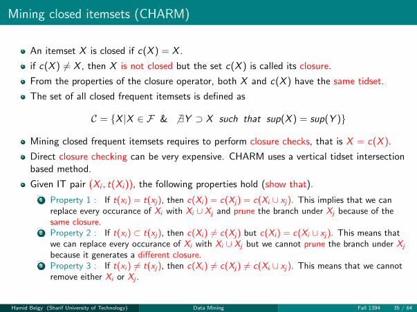
Mining closed itemsets (CHARM)

An itemset X is closed if c(X ) = X .

if c(X ) 6= X , then X is not closed but the set c(X ) is called its closure.

From the properties of the closure operator, both X and c(X ) have the same tidset.

The set of all closed frequent itemsets is defined as

C = {X |X ∈ F & 6 ∃Y ⊃ X such that sup(X ) = sup(Y )}

Mining closed frequent itemsets requires to perform closure checks, that is X = c(X ).

Direct closure checking can be very expensive. CHARM uses a vertical tidset intersectionbased method.

Given IT pair (Xi , t(Xi )), the following properties hold (show that).

1 Property 1 : If t(xi ) = t(xj), then c(Xi ) = c(Xj) = c(Xi ∪ xj). This implies that we canreplace every occurance of Xi with Xi ∪ Xj and prune the branch under Xj because of thesame closure.

2 Property 2 : If t(xi ) ⊂ t(xj), then c(Xi ) 6= c(Xj) but c(Xi ) = c(Xi ∪ xj). This means thatwe can replace every occurance of Xi with Xi ∪ Xj but we cannot prune the branch under Xj

because it generates a different closure.3 Property 3 : If t(xi ) 6= t(xj), then c(Xi ) 6= c(Xj) 6= c(Xi ∪ xj). This means that we cannot

remove either Xi or Xj .


Mining closed itemsets (CHARM)

CHARM takes the set of frequent single items along with their tidset as input (i.e.(Xi , t(Xi ))).

Initially the set of all closed itemsets C is empty.

Given any IT pair set P = {(Xi , t(Xi ))}, CHARM first sorts them in increasing order oftheir support counts.

For each itemset Xi , we try to extend it with all other items Xi in the sorted order andthen apply the given properties 1 and 2 to prune branches.

1 We make sure that Xij = Xi ∪ Xj is frequent.2 If Xij is frequent, then we check properties 1 and 2.

If Pi 6= φ, then CHARM is called using Pi .

If Xi is not subset of any closed set Z with the same support, we can safely add it to C.


Mining closed itemsets (CHARM algorithm)9.3 Mining Closed Frequent Itemsets: Charm Algorithm 249

ALGORITHM 9.2. Algorithm CHARM

// Initial Call: C←∅, P ←!

⟨i, t(i)⟩ : i ∈ I,sup(i)≥minsup"

CHARM (P , minsup, C):Sort P in increasing order of support (i.e., by increasing |t(Xi)|)1

foreach ⟨Xi , t(Xi )⟩ ∈ P do2

Pi←∅3

foreach ⟨Xj , t(Xj )⟩ ∈ P , with j > i do4

Xij = Xi ∪Xj5

t(Xij ) = t(Xi) ∩ t(Xj )6

if sup(Xij )≥minsup then7

if t(Xi) = t(Xj ) then // Property 18

Replace Xi with Xij in P and Pi9

Remove ⟨Xj , t(Xj )⟩ from P10

else11

if t(Xi)⊂ t(Xj ) then // Property 212

Replace Xi with Xij in P and Pi13

else // Property 314

Pi← Pi ∪!

⟨Xij , t(Xij )⟩"

15

if Pi ̸= ∅ then CHARM (Pi , minsup, C)16

if ̸ ∃Z ∈ C, such that Xi ⊆Z and t(Xi) = t(Z) then17

C = C ∪Xi // Add Xi to closed set18

it is pruned. AD is frequent and because t(A) ̸= t(D), we add ⟨AD,135⟩ to the setPA (property 3). When we combine A with E, property 2 applies, and we simplyreplace all occurrences of A in both P and PA with AE, which is illustrated with thestrike-through. Likewise, because t(A) ⊂ t(B) all current occurrences of A, actuallyAE, in both P and PA are replaced by AEB. The set PA thus contains only one itemset{⟨ADEB,135⟩}. When CHARM is invoked with PA as the IT-pair, it jumps straight toline 18, and adds ADEB to the set of closed itemsets C. When the call returns, wecheck whether AEB can be added as a closed itemset. AEB is a subset of ADEB,but it does not have the same support, thus AEB is also added to C. At this point allclosed itemsets containing A have been found.

The Charm algorithm proceeds with the remaining branches as shown inFigure 9.4b. For instance, C is processed next. CD is infrequent and thus pruned.CE is frequent and it is added to PC as a new extension (via property 3). Becauset(C) ⊂ t(B), all occurrences of C are replaced by CB, and PC = {⟨CEB,245⟩}. CEB

and CB are both found to be closed. The computation proceeds in this manner untilall closed frequent itemsets are enumerated. Note that when we get to DEB andperform the closure check, we find that it is a subset of ADEB and also has the samesupport; thus DEB is not closed.


Mining closed itemsets (CHARM example)

Execution of CHARM using the following database

8.1 Frequent Itemsets and Association Rules 219

D A B C D E

1 1 1 0 1 1

2 0 1 1 0 1

3 1 1 0 1 1

4 1 1 1 0 1

5 1 1 1 1 1

6 0 1 1 1 0

(a) Binary database

t i(t)

1 ABDE

2 BCE

3 ABDE

4 ABCE

5 ABCDE

6 BCD


x A B C D E

1 1 2 1 13 2 4 3 2

t(x) 4 3 5 5 35 4 6 6 4

5 56





sup(X,D) =!

!{t | ⟨t, i(t)⟩ ∈D and X⊆ i(t)}!

!= |t(X)|


rsup(X,D) =sup(X,D)

|D|





F (1) = {A,B,C,D,E}



F (4) = {ABDE}


A AE AEB

1345

C

2456

D

1356

E

12345

B

123456

AD ADE ADEB

135

PA

(a) Process A

A AE AEB C CB D DB E EB B

1345 2456 1356 12345 123456

AD ADE ADEB

135

PA

CE CEB

245

PC

DE DEB

135

PD

(b) Charm

Figure 9.4. Mining closed frequent itemsets. Closed itemsets are shown as shaded ovals. Strike-through

represents itemsets Xi replaced by Xi ∪Xj during execution of the algorithm. Infrequent itemsets are not

shown.

9.4 NONDERIVABLE ITEMSETS

An itemset is called nonderivable if its support cannot be deduced from the supportsof its subsets. The set of all frequent nonderivable itemsets is a summary or condensedrepresentation of the set of all frequent itemsets. Further, it is lossless with respect tosupport, that is, the exact support of all other frequent itemsets can be deduced from it.

Generalized ItemsetsLet T be a set of tids, let I be a set of items, and let X be a k-itemset, that is, X =

{x1,x2, . . . ,xk}. Consider the tidsets t(xi) for each item xi ∈X. These k-tidsets induce apartitioning of the set of all tids into 2k regions, some of which may be empty, whereeach partition contains the tids for some subset of items Y ⊆ X, but for none of theremaining items Z = Y \ X. Each such region is therefore the tidset of a generalized

itemset comprising items in X or their negations. As such a generalized itemset can berepresented as YZ, where Y consists of regular items and Z consists of negated items.We define the support of a generalized itemset YZ as the number of transactions that

Process PA


A AE AEB

1345

C

2456

D

1356

E

12345

B

123456

AD ADE ADEB

135

PA

(a) Process A

A AE AEB C CB D DB E EB B

1345 2456 1356 12345 123456

AD ADE ADEB

135

PA

CE CEB

245

PC

DE DEB

135

PD

(b) Charm

Figure 9.4. Mining closed frequent itemsets. Closed itemsets are shown as shaded ovals. Strike-through

represents itemsets Xi replaced by Xi ∪Xj during execution of the algorithm. Infrequent itemsets are not

shown.

9.4 NONDERIVABLE ITEMSETS

An itemset is called nonderivable if its support cannot be deduced from the supportsof its subsets. The set of all frequent nonderivable itemsets is a summary or condensedrepresentation of the set of all frequent itemsets. Further, it is lossless with respect tosupport, that is, the exact support of all other frequent itemsets can be deduced from it.

Generalized ItemsetsLet T be a set of tids, let I be a set of items, and let X be a k-itemset, that is, X =

{x1,x2, . . . ,xk}. Consider the tidsets t(xi) for each item xi ∈X. These k-tidsets induce apartitioning of the set of all tids into 2k regions, some of which may be empty, whereeach partition contains the tids for some subset of items Y ⊆ X, but for none of theremaining items Z = Y \ X. Each such region is therefore the tidset of a generalized

itemset comprising items in X or their negations. As such a generalized itemset can berepresented as YZ, where Y consists of regular items and Z consists of negated items.We define the support of a generalized itemset YZ as the number of transactions that

CHARM algorithm


Table of contents

1 Introduction




5 Sequence mining

6 Graph mining



Sequence mining

Many real-world applications such as bioinformatics, web mining, and text mining have todeal with sequential and temporal data.

Sequence mining helps discover patterns across time or positions in a given dataset.

Let Σ denote an alphabet, defined as a finite set of characters or symbols, and let |Σ|denote its cardinality.

A sequence or a string is defined as an ordered list of symbols, and is written ass = s1s2 . . . sk , where si ∈ Σ is a symbol at position i , also denoted as s[i ].

The length of sequence s is denoted by k = |s|. A sequence with length k is also called ak−sequence.

A substring s[i : j ] = si si+1 . . . sj−1sj is a sequence of consecutive symbols in positions ithrough j (for j > i).

A prefix of a sequence s is a substring of the form

s[1 : i ] = s1s2 . . . si ∀i ∈ [0, k].

A suffix of a sequence s is a substring of the form

s[i : k] = si si+1 . . . sk ∀i ∈ [0, n + 1].

String s[1 : 0] is empty prefix and string s[n + 1 : n] is empty suffix.


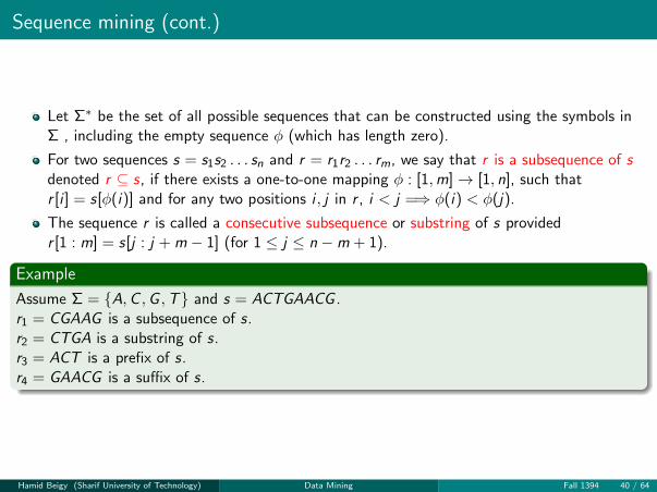
Sequence mining (cont.)

Let Σ∗ be the set of all possible sequences that can be constructed using the symbols inΣ , including the empty sequence φ (which has length zero).

For two sequences s = s1s2 . . . sn and r = r1r2 . . . rm, we say that r is a subsequence of sdenoted r ⊆ s, if there exists a one-to-one mapping φ : [1,m]→ [1, n], such thatr [i ] = s[φ(i)] and for any two positions i , j in r , i < j =⇒ φ(i) < φ(j).

The sequence r is called a consecutive subsequence or substring of s providedr [1 : m] = s[j : j + m − 1] (for 1 ≤ j ≤ n −m + 1).

Example

Assume Σ = {A,C ,G ,T} and s = ACTGAACG .r1 = CGAAG is a subsequence of s.r2 = CTGA is a substring of s.r3 = ACT is a prefix of s.r4 = GAACG is a suffix of s.


Sequence mining (cont.)

Given a database D = {s1, s2, . . . , sN} of N sequences, and given some sequence r ,sup(r) in the database D is defined as the total number of sequences in D that contain r .

sup(r) = |{si ∈ D|r ⊆ si}|Given a minsup, a sequence r is frequent if sup(r) ≥ minsup.

A frequent sequence is maximal if it is not a subsequence of any other frequent sequence.

A frequent sequence is closed if it is not a subsequence of any other frequent sequencewith the same support.


Mining frequent sequences

For sequence mining, he order of the symbols matters, and thus we have to consider allpossible permutations of the symbols as the possible frequent candidates.

The sequence search space can be organized in a prefix search tree.

The root of the tree (level 0) contains the empty sequence, with each symbol x ∈ Σ asone of its children.

A node labeled with the sequence s = s1s2 . . . sk at level k has children of the forms ′ = s1s2 . . . sksk+1 at level k + 1. s ′ is called an extension of s.


260 Sequence Mining

Given a database D = {s1,s2, . . . ,sN} of N sequences, and given some sequence r,the support of r in the database D is defined as the total number of sequences in D thatcontain r

sup(r) =!

!

!

"

si ∈D|r⊆ si

#

!

!

!

The relative support of r is the fraction of sequences that contain r

rsup(r) = sup(r)/N

Given a user-specified minsup threshold, we say that a sequence r is frequent indatabase D if sup(r) ≥ minsup. A frequent sequence is maximal if it is not asubsequence of any other frequent sequence, and a frequent sequence is closed if itis not a subsequence of any other frequent sequence with the same support.

10.2 MINING FREQUENT SEQUENCES

For sequence mining the order of the symbols matters, and thus we have to considerall possible permutations of the symbols as the possible frequent candidates. Contrastthis with itemset mining, where we had only to consider combinations of the items. Thesequence search space can be organized in a prefix search tree. The root of the tree, atlevel 0, contains the empty sequence, with each symbol x ∈! as one of its children. Assuch, a node labeled with the sequence s = s1s2 . . . sk at level k has children of the forms′ = s1s2 . . . sksk+1 at level k+1. In other words, s is a prefix of each child s′, which is alsocalled an extension of s.

Example 10.2. Let ! = {A,C,G,T} and let the sequence database D consist of thethree sequences shown in Table 10.1. The sequence search space organized as a prefixsearch tree is illustrated in Figure 10.1. The support of each sequence is shown withinbrackets. For example, the node labeled A has three extensions AA, AG, and AT,out of which AT is infrequent if minsup = 3.

The subsequence search space is conceptually infinite because it comprises allsequences in !∗, that is, all sequences of length zero or more that can be created usingsymbols in !. In practice, the database D consists of bounded length sequences. Let l

denote the length of the longest sequence in the database, then, in the worst case, wewill have to consider all candidate sequences of length up to l, which gives the following

Table 10.1. Example sequence database

Id Sequence

s1 CAGAAGT

s2 TGACAG

s3 GAAGT

1 Σ = {A,C ,G ,T}2 Sequence A has three extensions AA, AG , and AT .

3 If minsup = 3, AA and AG are frequent but AT isinfrequent.


Mining frequent sequences (cont.)

The search space for all subsequence is conceptually infinite because it comprises allsequences (with length zero or more) in Σ∗.

In practice, the database D consists of bounded length sequences. Let l denote the lengthof the longest sequence in the database.

In the worst case, we must consider all candidate sequences of length up to l , and the sizeof search space equals to

|Σ|1 + |Σ|2 + . . .+ |Σ|l = O(|Σ|l)where at level k , there are |Σ|k possible subsequences of length k.


Generalized equential pattern mining (GSP)

GSP searches the sequence prefix tree using a level-wise or breadth-first search.

Given the set of frequent sequences at level k , GSP generates all possible sequenceextensions or candidates at level k + 1.

Then GSP computes the support of each candidate and prunes infrequent sequences.

GSP stops search when no more frequent extensions are possible.

GSP uses monotonic property of support to prune candidate patters.

The computational complexity of GSP is O(|Σ|l).

The I/O complexity of GSP is O(l × D).


Generalized equential pattern mining (GSP)


260 Sequence Mining


sup(r) =!

!

!

"

si ∈D|r⊆ si

#

!

!

!


rsup(r) = sup(r)/N








Id Sequence

s1 CAGAAGT

s2 TGACAG

s3 GAAGT

The Sequence search space is (minsup = 3)262 Sequence Mining

∅(3)

A(3)

AA(3)

AAA(1) AAG(3)

AAGG

AG(3)

AGA(1) AGG(1)

AT(2)

C(2) G(3)

GA(3)

GAA(3)

GAAA GAAG(3)

GAG(3)

GAGA GAGG

GG(3)

GGA(0) GGG(0)

GT(2)

T(3)

TA(1) TG(1) TT(0)

Figure 10.1. Sequence search space: shaded ovals represent candidates that are infrequent; those without

support in brackets can be pruned based on an infrequent subsequence. Unshaded ovals represent frequent

sequences.

The pseudo-code for the level-wise, generalized sequential pattern (GSP) miningmethod is shown in Algorithm 10.1. It uses the antimonotonic property of support toprune candidate patterns, that is, no supersequence of an infrequent sequence can befrequent, and all subsequences of a frequent sequence must be frequent. The prefixsearch tree at level k is denoted C(k). Initially C(1) comprises all the symbols in !.Given the current set of candidate k-sequences C(k), the method first computes theirsupport (line 6). For each database sequence si ∈ D, we check whether a candidatesequence r ∈ C(k) is a subsequence of si . If so, we increment the support of r. Once thefrequent sequences at level k have been found, we generate the candidates for levelk + 1 (line 10). For the extension, each leaf ra is extended with the last symbol of anyother leaf rb that shares the same prefix (i.e., has the same parent), to obtain the newcandidate (k + 1)-sequence rab = ra + rb[k] (line 18). If the new candidate rab containsany infrequent k-sequence, we prune it.

Example 10.3. For example, let us mine the database shown in Table 10.1 usingminsup = 3. That is, we want to find only those subsequences that occur in allthree database sequences. Figure 10.1 shows that we begin by extending the emptysequence ∅ at level 0, to obtain the candidates A, C, G, and T at level 1. Out of theseC can be pruned because it is not frequent. Next we generate all possible candidatesat level 2. Notice that using A as the prefix we generate all possible extensionsAA, AG, and AT. A similar process is repeated for the other two symbols G andT. Some candidate extensions can be pruned without counting. For example, theextension GAAA obtained from GAA can be pruned because it has an infrequentsubsequence AAA. The figure shows all the frequent sequences (unshaded), out ofwhich GAAG(3) and T(3) are the maximal ones.

The computational complexity of GSP is O(|!|l) as per Eq. (10.1), where l is thelength of the longest frequent sequence. The I/O complexity is O(l · D) because wecompute the support of an entire level in one scan of the database.


Vertical sequences mining (SPADE)

The Spade algorithm uses a vertical database representation for sequence mining.

The idea is to record two items for each symbol:

1 The sequence identifier2 The position where it occures

Let L(s) be the set of such sequence-position tupples for smbole s, referred to as parlist.


260 Sequence Mining


sup(r) =!

!

!

"

si ∈D|r⊆ si

#

!

!

!


rsup(r) = sup(r)/N








Id Sequence

s1 CAGAAGT

s2 TGACAG

s3 GAAGT

1 A occures in s1 at positions 2, 4, and 5.

2 A occures in s2 at positions 3 and 5.

3 A occures in s3 at positions 2 and 3.

4 L(A) = {〈1, {2, 4, 5}〉, 〈2, {3, 5}〉〈3, {2, 3}〉}



Let L(s) be the set of such sequence-position tupples for smbole s, referred to as parlist.

L(s) for each s ∈ Σ represents its vertical representation.

Given k−sequence r , L(r) maintains the list of positions for the occurrences of the lastsymbol r [k] in each database sequence si , provided r ⊆ si .

The support of r is the number of distinct sequences in which r occures (sup(r) = |L(r)|).

SPADE uses the sequential join operation. Given L(a) and L(b) for k−sequences ra andrb. L(r) keeps the track of last symbol of r .

ra and rb are joinable if they share the same (k − 1)length prefix.

The main advantage of the vertical approach is that it enables different search strategiesover the sequence search space, including breadth or depth-first search.




260 Sequence Mining


sup(r) =!

!

!

"

si ∈D|r⊆ si

#

!

!

!


rsup(r) = sup(r)/N








Id Sequence

s1 CAGAAGT

s2 TGACAG

s3 GAAGT

Sequence mined via SPADE is (minsup = 3)

10.2 Mining Frequent Sequences 263

10.2.2 Vertical Sequence Mining: Spade

The Spade algorithm uses a vertical database representation for sequence mining.The idea is to record for each symbol the sequence identifiers and the positionswhere it occurs. For each symbol s ∈ !, we keep a set of tuples of the form⟨i,pos(s)⟩, where pos(s) is the set of positions in the database sequence si ∈ D

where symbol s appears. Let L(s) denote the set of such sequence-position tuplesfor symbol s, which we refer to as the poslist. The set of poslists for each symbols ∈ ! thus constitutes a vertical representation of the input database. In general,given k-sequence r, its poslist L(r) maintains the list of positions for the occurrencesof the last symbol r[k] in each database sequence si , provided r ⊆ si . The supportof sequence r is simply the number of distinct sequences in which r occurs, that is,sup(r) = |L(r)|.

Example 10.4. In Table 10.1, the symbol A occurs in s1 at positions 2, 4, and 5.Thus, we add the tuple ⟨1,{2,4,5}⟩ to L(A). Because A also occurs at positions 3and 5 in sequence s2, and at positions 2 and 3 in s3, the complete poslist for A is{⟨1,{2,4,5}⟩,⟨2,{3,5}⟩,⟨1,{2,3}⟩}. We have sup(A) = 3, as its poslist contains threetuples. Figure 10.2 shows the poslist for each symbol, as well as other sequences.For example, for sequence GT, we find that it is a subsequence of s1 and s3.

∅

A1 2,4,52 3,53 2,3

C1 12 4

G1 3,62 2,63 1,4

T1 72 13 5

AA1 4,52 53 3

AG1 3,62 63 4

AT1 73 5

GA1 4,52 3,53 2,3

GG1 62 63 4

GT1 73 5

TA2 3,5

TG2 2,6

AAA1 5

AAG1 62 63 4

AGA1 5

AGG1 6

GAA1 52 53 3

GAG1 62 63 4

GAAG1 62 63 4

Figure 10.2. Sequence mining via Spade: infrequent sequences with at least one occurrence are shown

shaded; those with zero support are not shown.


Table of contents

1 Introduction




5 Sequence mining

6 Graph mining



Graph mining (Introduction)

Graph data is becoming increasingly more ubiquitous in todays networked world.

Examples include social networks, cell phone networks, blogs, Internet, hyperlinkedstructure of WWW, bioinformatics, and semantic Web.

The goal of graph mining is to extract interesting subgraphs from a single large graph(such as a social network), or from a database of many graphs.

In different applications we may be interested in different kinds of subgraph patterns, suchas subtrees, complete graphs or cliques, bipartite cliques, anddense subgraphs.

These subgraphs may represent communities in a social network, hub and authority pageson the WWW, and cluster of proteins involved in similar biochemical functions.


Graphs

A graph is a pair G = (V ,E ) where V is a set of vertices, and E ⊆ V × V is a set ofedges. We assume that edges are unordered, so that the graph is undirected.

If (u, v) is an edge, we say that u and v are adjacent and that v is a neighbor of u, andvice versa.

The set of all neighbors of u in G is given as N(u) = {v ∈ V |(u, v) ∈ E}.A labeled graph has labels associated with its vertices as well as edges. We use L(u) todenote the label of the vertex u, and L(u, v) to denote the label of the edge (u, v).

Unlabeled graph11.1 Isomorphism and Support 281

v1 v2

v3 v4 v5v6

v7 v8(a)

a c

b a d c

b c

v1 v2

v3 v4 v5v6

v7 v8(b)

Figure 11.1. An unlabeled (a) and labeled (b) graph with eight vertices.

label set !V = {a,b,c,d}. In this example, edges are all assumed to be unlabeled,and are therefore edge labels are not shown. Considering Figure 11.1b, the label ofvertex v4 is L(v4) = a, and its neighbors are N(v4) = {v1,v2,v3,v5,v7,v8}. The edge(v4,v1) leads to the extended edge ⟨v4,v1,a,a⟩, where we omit the edge label L(v4,v1)

because it is empty.

SubgraphsA graph G′ = (V′,E′) is said to be a subgraph of G if V′ ⊆ V and E′ ⊆ E. Notethat this definition allows for disconnected subgraphs. However, typically data miningapplications call for connected subgraphs, defined as a subgraph G′ such that V′ ⊆ V,E′ ⊆E, and for any two nodes u,v ∈V′, there exists a path from u to v in G′.

Example 11.2. The graph defined by the bold edges in Figure 11.2a is a subgraphof the larger graph; it has vertex set V′ = {v1,v2,v4,v5,v6,v8}. However, it is adisconnected subgraph. Figure 11.2b shows an example of a connected subgraph onthe same vertex set V′.

Graph and Subgraph IsomorphismA graph G′ = (V′,E′) is said to be isomorphic to another graph G = (V,E) if thereexists a bijective function φ : V′ → V, i.e., both injective (into) and surjective (onto),such that

1. (u,v) ∈E′ ⇐⇒ (φ(u),φ(v)) ∈E

2. ∀u ∈V′, L(u) = L(φ(u))

3. ∀(u,v) ∈E′, L(u,v) = L(φ(u),φ(v))

In other words, the isomorphism φ preserves the edge adjacencies as well as the vertexand edge labels. Put differently, the extended tuple ⟨u,v,L(u),L(v),L(u,v)⟩ ∈G′ if andonly if ⟨φ(u),φ(v),L(φ(u)),L(φ(v)),L(φ(u),φ(v))⟩ ∈G.

Labeled graph11.1 Isomorphism and Support 281

v1 v2

v3 v4 v5v6

v7 v8(a)

a c

b a d c

b c

v1 v2

v3 v4 v5v6

v7 v8(b)

Figure 11.1. An unlabeled (a) and labeled (b) graph with eight vertices.

label set !V = {a,b,c,d}. In this example, edges are all assumed to be unlabeled,and are therefore edge labels are not shown. Considering Figure 11.1b, the label ofvertex v4 is L(v4) = a, and its neighbors are N(v4) = {v1,v2,v3,v5,v7,v8}. The edge(v4,v1) leads to the extended edge ⟨v4,v1,a,a⟩, where we omit the edge label L(v4,v1)

because it is empty.

SubgraphsA graph G′ = (V′,E′) is said to be a subgraph of G if V′ ⊆ V and E′ ⊆ E. Notethat this definition allows for disconnected subgraphs. However, typically data miningapplications call for connected subgraphs, defined as a subgraph G′ such that V′ ⊆ V,E′ ⊆E, and for any two nodes u,v ∈V′, there exists a path from u to v in G′.

Example 11.2. The graph defined by the bold edges in Figure 11.2a is a subgraphof the larger graph; it has vertex set V′ = {v1,v2,v4,v5,v6,v8}. However, it is adisconnected subgraph. Figure 11.2b shows an example of a connected subgraph onthe same vertex set V′.

Graph and Subgraph IsomorphismA graph G′ = (V′,E′) is said to be isomorphic to another graph G = (V,E) if thereexists a bijective function φ : V′ → V, i.e., both injective (into) and surjective (onto),such that

1. (u,v) ∈E′ ⇐⇒ (φ(u),φ(v)) ∈E

2. ∀u ∈V′, L(u) = L(φ(u))

3. ∀(u,v) ∈E′, L(u,v) = L(φ(u),φ(v))

In other words, the isomorphism φ preserves the edge adjacencies as well as the vertexand edge labels. Put differently, the extended tuple ⟨u,v,L(u),L(v),L(u,v)⟩ ∈G′ if andonly if ⟨φ(u),φ(v),L(φ(u)),L(φ(v)),L(φ(u),φ(v))⟩ ∈G.

Given an edge (u, v) ∈ G , the tuple 〈u, v , L(u), L(v), L(u, v)〉 that augments the edgewith the node and edge labels is called an extended edge.


Subggraphs

A graph G ′ = (V ′,E ′) is said to be a subgraph of G if V ′ ⊆ V and E ′ ⊆ E . Note thatthis definition allows for disconnected subgraphs.

Subgraph

282 Graph Pattern Mining

a c

b a d c

b c

v1 v2

v3 v4 v5v6

v7 v8(a)

a c

b a d c

b c

v1 v2

v3 v4 v5v6

v7 v8(b)

Figure 11.2. A subgraph (a) and connected subgraph (b).

u1 a

G1

u2 a

u3 b u4 b

v1 a

G2

v3 a

v2 b v4 b

w1 a

G3

w2 a

w3 b

x1 b

G4

x2 a

x3 b

Figure 11.3. Graph and subgraph isomorphism.

If the function φ is only injective but not surjective, we say that the mapping φ isa subgraph isomorphism from G′ to G. In this case, we say that G′ is isomorphic to asubgraph of G, that is, G′ is subgraph isomorphic to G, denoted G′ ⊆ G; we also saythat G contains G′.

Example 11.3. In Figure 11.3, G1 = (V1,E1) and G2 = (V2,E2) are isomorphic graphs.There are several possible isomorphisms between G1 and G2. An example of anisomorphism φ : V2→V1 is

φ(v1) = u1 φ(v2) = u3 φ(v3) = u2 φ(v4) = u4

The inverse mapping φ−1 specifies the isomorphism from G1 to G2. For example,φ−1(u1) = v1, φ−1(u2) = v3, and so on. The set of all possible isomorphisms from G2

to G1 are as follows:

v1 v2 v3 v4

φ1 u1 u3 u2 u4

φ2 u1 u4 u2 u3

φ3 u2 u3 u1 u4

φ4 u2 u4 u1 u3

Connected subgraph282 Graph Pattern Mining

a c

b a d c

b c

v1 v2

v3 v4 v5v6

v7 v8(a)

a c

b a d c

b c

v1 v2

v3 v4 v5v6

v7 v8(b)


u1 a

G1

u2 a

u3 b u4 b

v1 a

G2

v3 a

v2 b v4 b

w1 a

G3

w2 a

w3 b

x1 b

G4

x2 a

x3 b




φ(v1) = u1 φ(v2) = u3 φ(v3) = u2 φ(v4) = u4



v1 v2 v3 v4

φ1 u1 u3 u2 u4

φ2 u1 u4 u2 u3

φ3 u2 u3 u1 u4

φ4 u2 u4 u1 u3


Graph and subgraph isomorphism

A graph G ′ = (V ′,E ′) is said to be isomorphic to graph G = (V ,E ) if there exists afunction φ : V ′ → V such that

1 (u, v) ∈ E ′ ⇐⇒ (φ(u), φ(v)) ∈ E2 ∀u ∈ V ′, L(u) = L(φ(u))3 ∀(u, v) ∈ E ′, L(u, v) = L(φ(u), φ(v))


a c

b a d c

b c

v1 v2

v3 v4 v5v6

v7 v8(a)

a c

b a d c

b c

v1 v2

v3 v4 v5v6

v7 v8(b)


u1 a

G1

u2 a

u3 b u4 b

v1 a

G2

v3 a

v2 b v4 b

w1 a

G3

w2 a

w3 b

x1 b

G4

x2 a

x3 b




φ(v1) = u1 φ(v2) = u3 φ(v3) = u2 φ(v4) = u4



v1 v2 v3 v4

φ1 u1 u3 u2 u4

φ2 u1 u4 u2 u3

φ3 u2 u3 u1 u4

φ4 u2 u4 u1 u3


a c

b a d c

b c

v1 v2

v3 v4 v5v6

v7 v8(a)

a c

b a d c

b c

v1 v2

v3 v4 v5v6

v7 v8(b)


u1 a

G1

u2 a

u3 b u4 b

v1 a

G2

v3 a

v2 b v4 b

w1 a

G3

w2 a

w3 b

x1 b

G4

x2 a

x3 b




φ(v1) = u1 φ(v2) = u3 φ(v3) = u2 φ(v4) = u4



v1 v2 v3 v4

φ1 u1 u3 u2 u4

φ2 u1 u4 u2 u3

φ3 u2 u3 u1 u4

φ4 u2 u4 u1 u3


a c

b a d c

b c

v1 v2

v3 v4 v5v6

v7 v8(a)

a c

b a d c

b c

v1 v2

v3 v4 v5v6

v7 v8(b)


u1 a

G1

u2 a

u3 b u4 b

v1 a

G2

v3 a

v2 b v4 b

w1 a

G3

w2 a

w3 b

x1 b

G4

x2 a

x3 b




φ(v1) = u1 φ(v2) = u3 φ(v3) = u2 φ(v4) = u4



v1 v2 v3 v4

φ1 u1 u3 u2 u4

φ2 u1 u4 u2 u3

φ3 u2 u3 u1 u4

φ4 u2 u4 u1 u3


a c

b a d c

b c

v1 v2

v3 v4 v5v6

v7 v8(a)

a c

b a d c

b c

v1 v2

v3 v4 v5v6

v7 v8(b)


u1 a

G1

u2 a

u3 b u4 b

v1 a

G2

v3 a

v2 b v4 b

w1 a

G3

w2 a

w3 b

x1 b

G4

x2 a

x3 b




φ(v1) = u1 φ(v2) = u3 φ(v3) = u2 φ(v4) = u4



v1 v2 v3 v4

φ1 u1 u3 u2 u4

φ2 u1 u4 u2 u3

φ3 u2 u3 u1 u4

φ4 u2 u4 u1 u3


Subgraph support

Given a database of graphs,D = {G1,G2, . . . ,Gn},and given some graph G ,the support ofG in D is defined as follows:

sup(G ) = |{GI ∈ D|G ⊆ Gi}|

The support is simply the number of graphs in the database that contain G . Given aminsup threshold, the goal of graph mining is to mine all frequent connected subgraphswith sup(G ) ≥ minsup.

To mine all the frequent subgraphs, one has to search over the space of all possible graphpatterns, which is exponential in size.

There are two main challenges in frequent subgraph mining.1 The first challenge is to systematically generate candidate subgraphs. We use edge-growth as

the basic mechanism for extending the candidates.2 The second challenge is to count the support of a graph in the database. This involves

subgraph isomorphism checking, as we have to find the set of graphs that contain a givencandidate.


Candidate generation

An effective strategy to enumerate subgraph patterns is the called rightmost pathextension.

This algorithm performs DFS over its vertices, and create a DFS tree. Edges of DFS treeare called forward edges, and all other edges are called backward edges.

The rightmost path as the path from the root to the rightmost leaf (leaf with the highestindex in the DFS order).

Subgraph


11.2 CANDIDATE GENERATION

An effective strategy to enumerate subgraph patterns is the so-called rightmost path

extension. Given a graph G, we perform a depth-first search (DFS) over its vertices,and create a DFS spanning tree, that is, one that covers or spans all the vertices. Edgesthat are included in the DFS tree are called forward edges, and all other edges arecalled backward edges. Backward edges create cycles in the graph. Once we have aDFS tree, define the rightmost path as the path from the root to the rightmost leaf, thatis, to the leaf with the highest index in the DFS order.

Example 11.4. Consider the graph shown in Figure 11.4a. One of the possible DFSspanning trees is shown in Figure 11.4b (illustrated via bold edges), obtained bystarting at v1 and then choosing the vertex with the smallest index at each step.Figure 11.5 shows the same graph (ignoring the dashed edges), rearranged toemphasize the DFS tree structure. For instance, the edges (v1,v2) and (v2,v3) areexamples of forward edges, whereas (v3,v1), (v4,v1), and (v6,v1) are all backwardedges. The bold edges (v1,v5), (v5,v7) and (v7,v8) comprise the rightmost path.

For generating new candidates from a given graph G, we extend it by adding anew edge to vertices only on the rightmost path. We can either extend G by addingbackward edges from the rightmost vertex to some other vertex on the rightmost path(disallowing self-loops or multi-edges), or we can extend G by adding forward edgesfrom any of the vertices on the rightmost path. A backward extension does not add anew vertex, whereas a forward extension adds a new vertex.

For systematic candidate generation we impose a total order on the extensions, asfollows: First, we try all backward extensions from the rightmost vertex, and then wetry forward extensions from vertices on the rightmost path. Among the backward edgeextensions, if ur is the rightmost vertex, the extension (ur,vi) is tried before (ur,vj ) ifi < j . In other words, backward extensions closer to the root are considered beforethose farther away from the root along the rightmost path. Among the forward edgeextensions, if vx is the new vertex to be added, the extension (vi,vx) is tried before

v6 d c

v5

a v7

v1 a a v2 b v8

v4 c b v3

(a)

v6 d c

v5

a v7

v1 a a v2 b v8

v4 c b v3

(b)

Figure 11.4. A graph (a) and a possible depth-first spanning tree (b).

Connected subgraph


11.2 CANDIDATE GENERATION

An effective strategy to enumerate subgraph patterns is the so-called rightmost path

extension. Given a graph G, we perform a depth-first search (DFS) over its vertices,and create a DFS spanning tree, that is, one that covers or spans all the vertices. Edgesthat are included in the DFS tree are called forward edges, and all other edges arecalled backward edges. Backward edges create cycles in the graph. Once we have aDFS tree, define the rightmost path as the path from the root to the rightmost leaf, thatis, to the leaf with the highest index in the DFS order.

Example 11.4. Consider the graph shown in Figure 11.4a. One of the possible DFSspanning trees is shown in Figure 11.4b (illustrated via bold edges), obtained bystarting at v1 and then choosing the vertex with the smallest index at each step.Figure 11.5 shows the same graph (ignoring the dashed edges), rearranged toemphasize the DFS tree structure. For instance, the edges (v1,v2) and (v2,v3) areexamples of forward edges, whereas (v3,v1), (v4,v1), and (v6,v1) are all backwardedges. The bold edges (v1,v5), (v5,v7) and (v7,v8) comprise the rightmost path.

For generating new candidates from a given graph G, we extend it by adding anew edge to vertices only on the rightmost path. We can either extend G by addingbackward edges from the rightmost vertex to some other vertex on the rightmost path(disallowing self-loops or multi-edges), or we can extend G by adding forward edgesfrom any of the vertices on the rightmost path. A backward extension does not add anew vertex, whereas a forward extension adds a new vertex.

For systematic candidate generation we impose a total order on the extensions, asfollows: First, we try all backward extensions from the rightmost vertex, and then wetry forward extensions from vertices on the rightmost path. Among the backward edgeextensions, if ur is the rightmost vertex, the extension (ur,vi) is tried before (ur,vj ) ifi < j . In other words, backward extensions closer to the root are considered beforethose farther away from the root along the rightmost path. Among the forward edgeextensions, if vx is the new vertex to be added, the extension (vi,vx) is tried before

v6 d c

v5

a v7

v1 a a v2 b v8

v4 c b v3

(a)

v6 d c

v5

a v7

v1 a a v2 b v8

v4 c b v3

(b)

Figure 11.4. A graph (a) and a possible depth-first spanning tree (b).

The above DFS spanning tree obtained by starting at v1 and then choosing the vertexwith the smallest index at each step.


Candidate generation (cont.)

For systematic candidate generation, the following steps are done.First, we try all backward extensions from the rightmost vertex. Backward extensionscloser to the root are considered before those farther away from the root along therightmost path.Then, we try forward extensions from vertices on the rightmost path. The vertices fartherfrom the root are extended before those closer to the root.

11.2 Candidate Generation 285

v1 a

v2 a v5 c #6

v3 b v4 c v6 d v7 a #5

v8 b #4

#3

#1

#2

Figure 11.5. Rightmost path extensions. The bold path is the rightmost path in the DFS tree. The rightmost

vertex is v8, shown double circled. Solid black lines (thin and bold) indicate the forward edges, which are part

of the DFS tree. The backward edges, which by definition are not part of the DFS tree, are shown in gray.

The set of possible extensions on the rightmost path are shown with dashed lines. The precedence ordering

of the extensions is also shown.

(vj ,vx) if i > j . In other words, the vertices farther from the root (those at greaterdepth) are extended before those closer to the root. Also note that the new vertex willbe numbered x = r + 1, as it will become the new rightmost vertex after the extension.

Example 11.5. Consider the order of extensions shown in Figure 11.5. Node v8 is therightmost vertex; thus we try backward extensions only from v8. The first extension,denoted #1 in Figure 11.5, is the backward edge (v8,v1) connecting v8 to the root,and the next extension is (v8,v5), denoted #2, which is also backward. No otherbackward extensions are possible without introducing multiple edges between thesame pair of vertices. The forward extensions are tried in reverse order, starting fromthe rightmost vertex v8 (extension denoted as #3) and ending at the root (extensiondenoted as #6). Thus, the forward extension (v8,vx), denoted #3, comes before theforward extension (v7,vx), denoted #4, and so on.

11.2.1 Canonical Code

When generating candidates using rightmost path extensions, it is possible thatduplicate, that is, isomorphic, graphs are generated via different extensions. Amongthe isomorphic candidates, we need to keep only one for further extension, whereas theothers can be pruned to avoid redundant computation. The main idea is that if we cansomehow sort or rank the isomorphic graphs, we can pick the canonical representative,say the one with the least rank, and extend only that graph.


Canonical Code

When generating candidates using rightmost path extensions, it is possible that duplicate,that is, isomorphic, graphs are generated via different extensions.Among the isomorphic candidates, we need to keep only one for further extension,whereas the others can be pruned to avoid redundant computation.The main idea is that if we can somehow sort or rank the isomorphic graphs, we can pickthe canonical representative.The DFS code of G is used for canonical representation and denoted by DFScode(G ), isdefined as the sequence of extended edge tuples of form 〈vi , vj , L(vi ), L(vj), L(vi , vj)〉listed in the DFS edge order.286 Graph Pattern Mining

v1 a

G1

v2 a

v3 a b v4

q

r r

r

v1 a

G2

v2 a

v3 b a v4

q

r r

r

v1 a

G3

v2 a b v4

v3 a

q

r

r

r

t11 = ⟨v1,v2,a,a,q⟩

t12 = ⟨v2,v3,a,a,r⟩

t13 = ⟨v3,v1,a,a,r⟩

t14 = ⟨v2,v4,a,b,r⟩

t21 = ⟨v1,v2,a,a,q⟩

t22 = ⟨v2,v3,a,b,r⟩

t23 = ⟨v2,v4,a,a,r⟩

t24 = ⟨v4,v1,a,a,r⟩

t31 = ⟨v1,v2,a,a,q⟩

t32 = ⟨v2,v3,a,a,r⟩

t33 = ⟨v3,v1,a,a,r⟩

t34 = ⟨v1,v4,a,b,r⟩

DFScode(G1) DFScode(G2) DFScode(G3)

Figure 11.6. Canonical DFS code. G1 is canonical, whereas G2 and G3 are noncanonical. Vertex label set

!V = {a,b}, and edge label set !E = {q,r}. The vertices are numbered in DFS order.

Let G be a graph and let TG be a DFS spanning tree for G. The DFS tree TG

defines an ordering of both the nodes and edges in G. The DFS node ordering isobtained by numbering the nodes consecutively in the order they are visited in theDFS walk. We assume henceforth that for a pattern graph G the nodes are numberedaccording to their position in the DFS ordering, so that i < j implies that vi comesbefore vj in the DFS walk. The DFS edge ordering is obtained by following the edgesbetween consecutive nodes in DFS order, with the condition that all the backwardedges incident with vertex vi are listed before any of the forward edges incident with it.The DFS code for a graph G, for a given DFS tree TG, denoted DFScode(G), is definedas the sequence of extended edge tuples of the form

!

vi,vj ,L(vi),L(vj ),L(vi,vj )"

listedin the DFS edge order.

Example 11.6. Figure 11.6 shows the DFS codes for three graphs, which are allisomorphic to each other. The graphs have node and edge labels drawn from thelabel sets !V = {a,b} and !E = {q,r}. The edge labels are shown centered on theedges. The bold edges comprise the DFS tree for each graph. For G1, the DFS nodeordering is v1,v2,v3,v4, whereas the DFS edge ordering is (v1,v2), (v2,v3), (v3,v1),and (v2,v4). Based on the DFS edge ordering, the first tuple in the DFS code for G1

is therefore ⟨v1,v2,a,a,q⟩. The next tuple is ⟨v2,v3,a,a,r⟩ and so on. The DFS codefor each graph is shown in the corresponding box below the graph.

Canonical DFS CodeA subgraph is canonical if it has the smallest DFS code among all possible isomorphicgraphs, with the ordering between codes defined as follows. Let t1 and t2 be any two


Canonical Code (cont.)

A subgraph is canonical if it has the smallest DFS code among all possible isomorphicgraphs.

Let t1 and t2 be any two DFS code tuples:

t1 = 〈vi , vj , L(vi ), L(vj), L(vi , vj)〉t2 = 〈vx , vy , L(vx), L(vy ), L(vx , vy )〉

We say that t1 is smaller than t2, written t1 < t2, iff1 (vi , vj) <e (vx , vy ) or2 (vi , vj) = (vx , vy ) and 〈L(vi ), L(vj), L(vi , vj)〉 <l 〈L(vx), L(vy ), L(vx , vy )〉.

Let eij = (vi , vj) and exy = (vx , vy ) be any two edges. We say that eij <e exy iff1 If eij and exy are both forward edges, then (a) j < y , or (b) j = y and i > x .2 If eij and exy are both backward edges, then (a) i < x , or (b) i = x and j < y .3 If eij is a forward and exy is a backward edge, then j ≤ x .4 If eij is a backward and exy is a forward edge, then i < y .


Canonical Code (cont.)


v1 a

G1

v2 a

v3 a b v4

q

r r

r

v1 a

G2

v2 a

v3 b a v4

q

r r

r

v1 a

G3

v2 a b v4

v3 a

q

r

r

r

t11 = ⟨v1,v2,a,a,q⟩

t12 = ⟨v2,v3,a,a,r⟩

t13 = ⟨v3,v1,a,a,r⟩

t14 = ⟨v2,v4,a,b,r⟩

t21 = ⟨v1,v2,a,a,q⟩

t22 = ⟨v2,v3,a,b,r⟩

t23 = ⟨v2,v4,a,a,r⟩

t24 = ⟨v4,v1,a,a,r⟩

t31 = ⟨v1,v2,a,a,q⟩

t32 = ⟨v2,v3,a,a,r⟩

t33 = ⟨v3,v1,a,a,r⟩

t34 = ⟨v1,v4,a,b,r⟩

DFScode(G1) DFScode(G2) DFScode(G3)

Figure 11.6. Canonical DFS code. G1 is canonical, whereas G2 and G3 are noncanonical. Vertex label set

!V = {a,b}, and edge label set !E = {q,r}. The vertices are numbered in DFS order.

Let G be a graph and let TG be a DFS spanning tree for G. The DFS tree TG

defines an ordering of both the nodes and edges in G. The DFS node ordering isobtained by numbering the nodes consecutively in the order they are visited in theDFS walk. We assume henceforth that for a pattern graph G the nodes are numberedaccording to their position in the DFS ordering, so that i < j implies that vi comesbefore vj in the DFS walk. The DFS edge ordering is obtained by following the edgesbetween consecutive nodes in DFS order, with the condition that all the backwardedges incident with vertex vi are listed before any of the forward edges incident with it.The DFS code for a graph G, for a given DFS tree TG, denoted DFScode(G), is definedas the sequence of extended edge tuples of the form

!

vi,vj ,L(vi),L(vj ),L(vi,vj )"

listedin the DFS edge order.

Example 11.6. Figure 11.6 shows the DFS codes for three graphs, which are allisomorphic to each other. The graphs have node and edge labels drawn from thelabel sets !V = {a,b} and !E = {q,r}. The edge labels are shown centered on theedges. The bold edges comprise the DFS tree for each graph. For G1, the DFS nodeordering is v1,v2,v3,v4, whereas the DFS edge ordering is (v1,v2), (v2,v3), (v3,v1),and (v2,v4). Based on the DFS edge ordering, the first tuple in the DFS code for G1

is therefore ⟨v1,v2,a,a,q⟩. The next tuple is ⟨v2,v3,a,a,r⟩ and so on. The DFS codefor each graph is shown in the corresponding box below the graph.

Canonical DFS CodeA subgraph is canonical if it has the smallest DFS code among all possible isomorphicgraphs, with the ordering between codes defined as follows. Let t1 and t2 be any two


gSpan algorithm (cont.)

Consider the following graph database comprising G1 and G2

11.3 The gSpan Algorithm 289

G1

a10

b20 a30

b40

G2

b50

a60 b70

a80

Figure 11.7. Example graph database.

Example 11.8. Consider the example graph database comprising G1 and G2 shownin Figure 11.7. Let minsup = 2, that is, assume that we are interested in miningsubgraphs that appear in both the graphs in the database. For each graph the nodelabels and node numbers are both shown, for example, the node a10 in G1 means thatnode 10 has label a.

Figure 11.8 shows the candidate patterns enumerated by gSpan. For eachcandidate the nodes are numbered in the DFS tree order. The solid boxes showfrequent subgraphs, whereas the dotted boxes show the infrequent ones. The dashedboxes represent noncanonical codes. Subgraphs that do not occur even once are notshown. The figure also shows the DFS codes and their corresponding graphs.

The mining process begins with the empty DFS code C0 corresponding to theempty subgraph. The set of possible 1-edge extensions comprises the new set ofcandidates. Among these, C3 is pruned because it is not canonical (it is isomorphic toC2), whereas C4 is pruned because it is not frequent. The remaining two candidates,C1 and C2, are both frequent and canonical, and are thus considered for furtherextension. The depth-first search considers C1 before C2, with the rightmost pathextensions of C1 being C5 and C6. However, C6 is not canonical; it is isomorphicto C5, which has the canonical DFS code. Further extensions of C5 are processedrecursively. Once the recursion from C1 completes, gSpan moves on to C2, which willbe recursively extended via rightmost edge extensions as illustrated by the subtreeunder C2. After processing C2, gSpan terminates because no other frequent andcanonical extensions are found. In this example, C12 is a maximal frequent subgraph,that is, no supergraph of C12 is frequent.

This example also shows the importance of duplicate elimination via canonicalchecking. The groups of isomorphic subgraphs encountered during the execution ofgSpan are as follows: {C2,C3}, {C5,C6,C17}, {C7,C19}, {C9,C25}, {C20,C21,C22,C24},and {C12,C13,C14}. Within each group the first graph is canonical and thus theremaining codes are pruned.

For a complete description of gSpan we have to specify the algorithm forenumerating the rightmost path extensions and their support, so that infrequentpatterns can be eliminated, and the procedure for checking whether a given DFS codeis canonical, so that duplicate patterns can be pruned. These are detailed next.

Let minsup = 2, that is, assume that we are interested in mining subgraphs that appearin both the graphs in the database.


gSpan algorithm (cont.)

C0

∅

C1

⟨0,1,a,a⟩

a0

a1

C2

⟨0,1,a,b⟩

a0

b1

C3

⟨0,1,b,a⟩

b0

a1

C4

⟨0,1,b,b⟩

b0

b1

C5

⟨0,1,a,a⟩

⟨1,2,a,b⟩

a0

a1

b2

C6

⟨0,1,a,a⟩

⟨0,2,a,b⟩

a0

a1 b2

C15

⟨0,1,a,b⟩

⟨1,2,b,a⟩

a0

b1

a2

C16

⟨0,1,a,b⟩

⟨1,2,b,b⟩

a0

b1

b2

C17

⟨0,1,a,b⟩

⟨0,2,a,a⟩

a0

b1 a2

C18

⟨0,1,a,b⟩

⟨0,2,a,b⟩

a0

b1 b2

C7

⟨0,1,a,a⟩

⟨1,2,a,b⟩

⟨2,0,b,a⟩

a0

a1

b2

C8

⟨0,1,a,a⟩

⟨1,2,a,b⟩

⟨2,3,b,b⟩

a0

a1

b2

b3

C9

⟨0,1,a,a⟩

⟨1,2,a,b⟩

⟨1,3,a,b⟩

a0

a1

b2 b3

C10

⟨0,1,a,a⟩

⟨1,2,a,b⟩

⟨0,3,a,b⟩

a0

a1 b3

b2

C24

⟨0,1,a,b⟩

⟨0,2,a,b⟩

⟨2,3,b,a⟩

a0

b1 b2

a3

C25

⟨0,1,a,b⟩

⟨0,2,a,b⟩

⟨0,3,a,a⟩

a0

b1 b2 a3

C19

⟨0,1,a,b⟩

⟨1,2,b,a⟩

⟨2,0,a,b⟩

a0

b1

a2

C20

⟨0,1,a,b⟩

⟨1,2,b,a⟩

⟨2,3,a,b⟩

a0

b1

a2

b3

C21

⟨0,1,a,b⟩

⟨1,2,b,a⟩

⟨1,3,b,b⟩

a0

b1

a2 b3

C22

⟨0,1,a,b⟩

⟨1,2,b,a⟩

⟨0,3,a,b⟩

a0

b1 b3

a2

C11

⟨0,1,a,a⟩

⟨1,2,a,b⟩

⟨2,0,b,a⟩

⟨2,3,b,b⟩

a0

a1

b2

b3

C12

⟨0,1,a,a⟩

⟨1,2,a,b⟩

⟨2,0,b,a⟩

⟨1,3,a,b⟩

a0

a1

b2 b3

C13

⟨0,1,a,a⟩

⟨1,2,a,b⟩

⟨2,0,b,a⟩

⟨0,3,a,b⟩

a0

a1 b3

b2

C14

⟨0,1,a,a⟩

⟨1,2,a,b⟩

⟨1,3,a,b⟩

⟨3,0,b,a⟩

a0

a1

b2 b3

C23

⟨0,1,a,b⟩

⟨1,2,b,a⟩

⟨2,3,a,b⟩

⟨3,1,b,b⟩

a0

b1

a2

b3

Figure 11.8. Frequent graph mining: minsup = 2. Solid boxes indicate the frequent subgraphs, dotted the

infrequent, and dashed the noncanonical subgraphs.


Table of contents

1 Introduction




5 Sequence mining

6 Graph mining



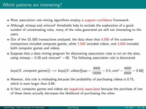
Which patterns are interesting?

Most association rule mining algorithms employ a support-confidence framework.

Although minsup and minconf thresholds help to exclude the exploration of a goodnumber of uninteresting rules, many of the rules generated are still not interesting to theusers.

Out of the 10, 000 transactions analyzed, the data show that 6,000 of the customertransactions included computer games, while 7,500 included videos, and 4,000 includedboth computer games and videos.

Suppose that a data mining program for discovering association rules is run on the data,using minsup = 0.30 and minconf = 60. The following association rule is discovered:

buys(X , computer games)) =⇒ buys(X , videos)[sup =4000

10000= 0.4, conf =

4000

6000= 0.66]

However, this rule is misleading because the probability of purchasing videos is 0.75,which is even larger than 0.66.

In fact, computer games and videos are negatively associated because the purchase of oneof these items actually decreases the likelihood of purchasing the other.


Which patterns are interesting?

Support and confidence measures are insufficient at filtering out uninteresting associationrules.

To tackle this weakness, a correlation measure can be used to augment thesupportconfidence framework for association rules. This leads to correlation rules of theform

A =⇒ B[support, confidence, correlation]

This is, a correlation rule is measured not only by its support and confidence but also bythe correlation between itemsets A and B.

There are many different correlation measures from which to choose.

1 Lift measure

lift(A,B) =P(A ∪ B)

P(A)P(B)

2 χ2 measure


Pattern evaluation measures

Instead of using the simple supportconfidence framework to evaluate frequent patterns,other measures, such as lift and χ2, often disclose more intrinsic pattern relationships.

How effective are these measures?1 Given two itemsets, A and B, all-confidence measure of A and B is defined as

all − confidence(A,B) = min[P(A|B),P(B|A)]

2 Given two itemsets, A and B, max-confidence measure of A and B is defined as

max − confidence(A,B) = max[P(A|B),P(B|A)]

3 Given two itemsets, A and B, Kulczynski measure of A and B is defined as

Kulczynski(A,B) =1

2[P(A|B) + P(B|A)]

4 Given two itemsets, A and B, cosine measure of A and B is defined as

cosine(A,B) =√

P(A|B)× P(B|A)

Values of these measures are only influenced by the supports of A, B, and A ∪ B, but notby the total number of transactions.

These measures range from 0 to 1, and the higher the value, the closer the relationshipbetween A and B.


Pattern evaluation measures (cont.)

Which is the best in assessing the discovered pattern relationships?

A null-transaction is a transaction that does not contain any of the itemsets beingexamined.

A measure is null-invariant if its value is free from the influence of null-transactions.Null-invariance is an important property for measuring association patterns in largetransaction databases.

Among the six discussed measures in this subsection, only lift and χ2 are notnull-invariant measures.

Among the all-confidence, max-confidence, Kulczynski, and cosine measures, which isbest at indicating interesting pattern relationships?

Imbalance ratio (IR), which assesses the imbalance of two itemsets, A and B, in ruleimplications.

IR(A,B) =|sup(A)− sup(B)|

sup(A) + sup(B)− sup(A ∪ B)

If the two directional implications between A and B are the same, then IR(A,B) will bezero. Otherwise, the larger the difference between the two, the larger the imbalance ratio.

The imbalance ratio is independent of the number of null-transactions and independent ofthe total number of transactions.


Documents

Data Mining - Sharifce.sharif.edu/courses/94-95/1/ce714-1/resources/... · 244 Chapter 6 Mining Frequent Patterns, Associations, and Correlations ... co-occurring terms have numerous